Hydrography90m: a new high-resolution global hydrographic dataset

The geographic distribution of streams and rivers drives a multitude of patterns and processes in hydrology, geomorphology, geography, and ecology. Therefore, a hydrographic network that accurately delineates both small streams and large rivers, along with their topographic and topological properties, with equal precision would be indispensable in the earth sciences. Currently, available global hydrographies do not feature small headwater streams in great detail. However, these headwaters are vital because they are estimated to contribute to more than 70 % of overall stream length. We aimed to fill this gap by using the MERIT Hydro digital elevation model at 3 arcsec (∼90 m at the Equator) to derive a globally seamless, standardised hydrographic network, the “Hydrography90m”, with corresponding stream topographic and topological information. A central feature of the network is the minimal upstream contributing area, i.e. flow accumulation, of 0.05 km² (or 5 ha) to initiate a stream channel, which allowed us to extract headwater stream channels in great detail. By employing a suite of GRASS GIS hydrological modules, we calculated the range-wide upstream flow accumulation and flow direction to delineate a total of 1.6 million drainage basins and extracted globally a total of 726 million unique stream segments with their corresponding sub-catchments. In addition, we computed stream topographic variables comprising stream slope, gradient, length, and curvature attributes as well as stream topological variables to allow for network routing and various stream order classifications. We validated the spatial accuracy and flow accumulation of Hydrography90m against NHDPlus HR, an independent, national high-resolution hydrographic network dataset of the United States. Our validation shows that the newly developed Hydrography90m has the highest spatial precision and contains more headwater stream channels compared to three other global hydrographic datasets. This comprehensive approach provides a vital and long-overdue baseline for assessing actual streamflow in headwaters and opens new research avenues for high-resolution studies of surface water worldwide. Hydrography90m thus offers significant potential to facilitate the assessment of freshwater quantity and quality, inundation risk, biodiversity, conservation, and resource management objectives in a globally comprehensive and standardised manner. The Hydrography90m layers are available at https://doi.org/10.18728/igb-fred-762.1 (Amatulli et al., 2022a), and while they can be used directly in standard GIS applications, we recommend the seamless integration with hydrological modules in open-source QGIS and GRASS GIS software to further customise the data and derive optimal utility from it.

1 Introduction

Global information on spatial hydrographic attributes, including stream topographic and topological properties, is fundamental to numerous disciplines, such as hydrological and hydraulic studies, flood and drought impact investigations, agricultural and land management, freshwater ecosystem and biodiversity assessments, conservation, and element cycling, as well as for investigating the effects of climate change on the earth's freshwater resources (Lowe and Likens, 2005; Thoms et al., 2018; Maasri et al., 2021a). These hydrographic attributes contain the geographic location and distribution of the world's streams and rivers along with their network topologies and catchments.

The delineation of a hydrographic network across a wide geographic range is based on remotely sensed digital elevation models (DEMs). From such datasets it is possible to derive potential water flow channels, given that water follows the steepest downstream slope (Seibert and McGlynn, 2007). Defining the upstream contributing area, i.e. flow accumulation, that initiates a stream channel is central to delineating the streams within a hydrographic network. The smaller the threshold applied to the flow accumulation, the more detailed the resulting network and its headwaters.

Various DEMs have been used for global stream channelisation, beginning with the GTOPO30 DEM at 30 arcsec (∼1 km at the Equator) (USGS, 1996), from which the US Geological Survey (USGS) created the HYDRO1k dataset (USGS EROS Archive, 2018), using a 1 000 km² threshold of upstream contributing areas. Then, in the year 2000, based on the Shuttle Radar Topography Mission (SRTM) DEM (USGS, 2015) with a near-global, sub-60^∘latitude coverage at 3 arcsec (∼90 m at the Equator) spatial resolution, Lehner et al. (2008) delineated the first near-global HydroSHEDS river network at 7.5×7.5 arcsec (∼500 m at the Equator) spatial resolution, with a minimum of 10 km² upstream contributing area. This hydrographic dataset was later revised as the global HydroRIVERS product that used HYDRO1k for the northern latitudes. Subsequently, Yamazaki et al. (2019) computed stream channels and river widths together with flow accumulation and direction, with a stream channelisation threshold of 5 km², based on the 3×3 arcsec Multi-Error-Removed Improved-Terrain (MERIT) Hydro DEM. Recently, Lin et al. (2021) computed the MERIT Hydro–Vector hydrography dataset, which features global variable drainage density and was derived from the Multi-Error-Removed Improved-Terrain (MERIT) Hydro DEM (Yamazaki et al., 2019). Despite employing MERIT Hydro at 3×3 arcsec, the channelisation of the MERIT Hydro–Vector dataset was initialised using a 1 km² threshold for the upstream contributing area, followed by a machine learning procedure to trim network density. While MERIT Hydro–Vector features an up-to-date hydrographic network (i.e. stream channels) in the highest available global spatial resolution at 3×3 arcsec, its coarse channelisation threshold does not yield a worldwide distribution of small headwater stream channels in substantial detail.

High spatial resolution of hydrographic data is key for informed water management, as it offers a detailed distribution of stream and river channels and thus enables accurate discharge and biogeochemical cycling simulations, (Marzadri et al., 2021; Liu et al., 2021; Hosen et al., 2021), nutrient concentration estimations (Shen et al., 2020), as well as biodiversity and environmental protection (Benstead and Leigh, 2012; Domisch et al., 2015a; Jackson et al., 2016). In addition, it allows for the delineation of small streams and their headwaters, i.e. the first and second Strahler order streams (Strahler, 1957). These streams are estimated to comprise >70 % of the overall length of a hydrographic network (Lowe and Likens, 2005; Leopold et al., 1964; Benstead and Leigh, 2012) and contribute significantly to flow and nutrient dynamics (Shumilova et al., 2019; Shanafield et al., 2021) that are essential for maintaining biodiversity-rich habitats (Finn et al., 2011; Meyer et al., 2007). Delineating stream channels at a high spatial resolution also allows for the assessment of the distribution of ephemeral streams, i.e. intermittent streams that run dry in certain seasons (Datry et al., 2014). While Messager et al. (2021) have mapped the global distribution of such non-perennial streams based on HydroRIVERS, small headwater streams are nevertheless missing from this dataset because of a significantly larger stream channelisation threshold, as mentioned in the preceding paragraph.

With Hydrography90m, we address the all-important issue of headwaters and present a globally seamless and standardised hydrographic network at 3×3 arcsec (equal $\mathrm{0.0008}\stackrel{\mathrm{‾}}{\mathrm{3}}{}^{\circ }$) together with their corresponding stream topographic and topological attributes. We use the Multi-Error-Removed Improved-Terrain (MERIT) Hydro DEM (Yamazaki et al., 2019) and employ a standard, worldwide channelisation threshold of 0.05 km² (or six 3×3 arcsec grid cells at the Equator). This results in a dense network, which depicts small headwater stream channels in fine detail. This choice of small channelisation threshold (in the low hectare range) is fundamental in computing headwater stream variables, which are essential for intermittent and flood flow modelling (Ågren et al., 2015). Thus, thresholding with a higher value (e.g. 1 km²) would fail to include vital headwater stream hydrographic features.

The Hydrography90m dataset consists of a global rendition of stream channels and drainage basins, the sub-catchment of each stream segment, in-stream and among-stream distance metrics, and various stream slope and stream order metrics. Additionally, the dataset provides a full topology for flow routing, owing to unique stream segment identifiers, each of which contains the attributes of the related upstream and downstream segments. The Hydrography90m stream network and flow accumulation have been validated against the National Hydrography Dataset Plus High Resolution (NHDPlus HR) (Moore et al., 2019) product, revealing high precision on the spatial accuracy and flow accumulation computation. We note that we are in the process of providing monthly discharge estimates for each stream segment, which will be used to reduce the channel density so as to retain only those channels that have potentially held water during a given time frame within a 30-year period. The hydrographic dataset (https://doi.org/10.18728/igb-fred-762.1, Amatulli et al., 2022a) is available for download in raster and vector formats. We recommend downloading the data via http://hydrography.org (last access: 5 October 2022), where users can click on a map interface to choose the required tile to directly download the corresponding layers or follow a scripting procedure for batch download and subsequent processing (likewise available at http://hydrography.org last access: 5 October 2022).

2 Methodology

2.1 Terminology used

To facilitate the understanding of the various layers, we provide a description of terms used in the manuscript and Hydrography90m dataset (Fig. 1) below.

• Flow direction. The direction of water flow in a grid cell, given that water follows the steepest downstream slope.

• Flow accumulation. The upstream contributing area, i.e. the drainage of water into a given downstream cell. It is expressed in area units (in our case in km²)

• Flow accumulation threshold. The upstream contributing area that initiates a stream channel. In Hydrography90m, it has been set to 0.05 km² (∼ six 3” arcsec cells at the Equator).

• Stream cell. The grid cell that marks a stream channel's presence. It is the smallest spatial unit in Hydrography90m, with a size of 3×3 arcsec (equal to $\sim \mathrm{90}\times \mathrm{90}$ m at the equator).

• Stream channel. Part of the hydrographic network, as extracted from the DEM. A stream channel consists of many stream segments. In Hydrography90m the stream channel network does not assume the presence of water but indicates a potential flow path.

• Stream segment. The stream channel between two segment nodes (or from initialisation to the first confluence) of the network where the stream order is unchanged. Each stream segment worldwide is labelled with a unique ID.

• Drainage basin. Any area of land where precipitation collects and drains into a common outlet. The outlet can be into the sea or an inland depression. If the drainage basin can be included completely in one tile, it is labelled entire drainage basin, but if it intersects a tile border, it is termed truncated drainage basin. Each drainage basin worldwide is assigned a unique ID. Adjacent basins share a border that corresponds to the basin drainage divide (i.e. ridgeline between basins).

• Sub-catchment. Land area between two segment nodes that contributes to the local flow accumulation of a given stream segment. Sub-catchments and stream segments have a common unique ID worldwide. Adjacent sub-catchments share a border that corresponds to the sub-catchment drainage divide, i.e. the ridgeline between sub-catchments.

• Base layers. Comprise raster flow accumulation and flow direction, which are the primary layers for extracting the hydrographic network and basins.

• Network layers. Raster and vector layers that are derived from flow accumulation and flow direction. The network layers include drainage basins, sub-catchments, and stream segments.

• Topographic and topological variables. Additional attributes characterising the topography (e.g. stream slope, stream distance) and topology (e.g. stream order) of the hydrographic network at the stream cell or segment resolution.

• Tiling system. Two vector layers that consist of the irregular tiling system (ITS) and regular tiling system (RTS), used to derive the Hydrography90m.

• Regional unit. An area that contains only entire drainage basins, masking the truncated ones. Useful for selecting entire drainage basins towards custom study areas.

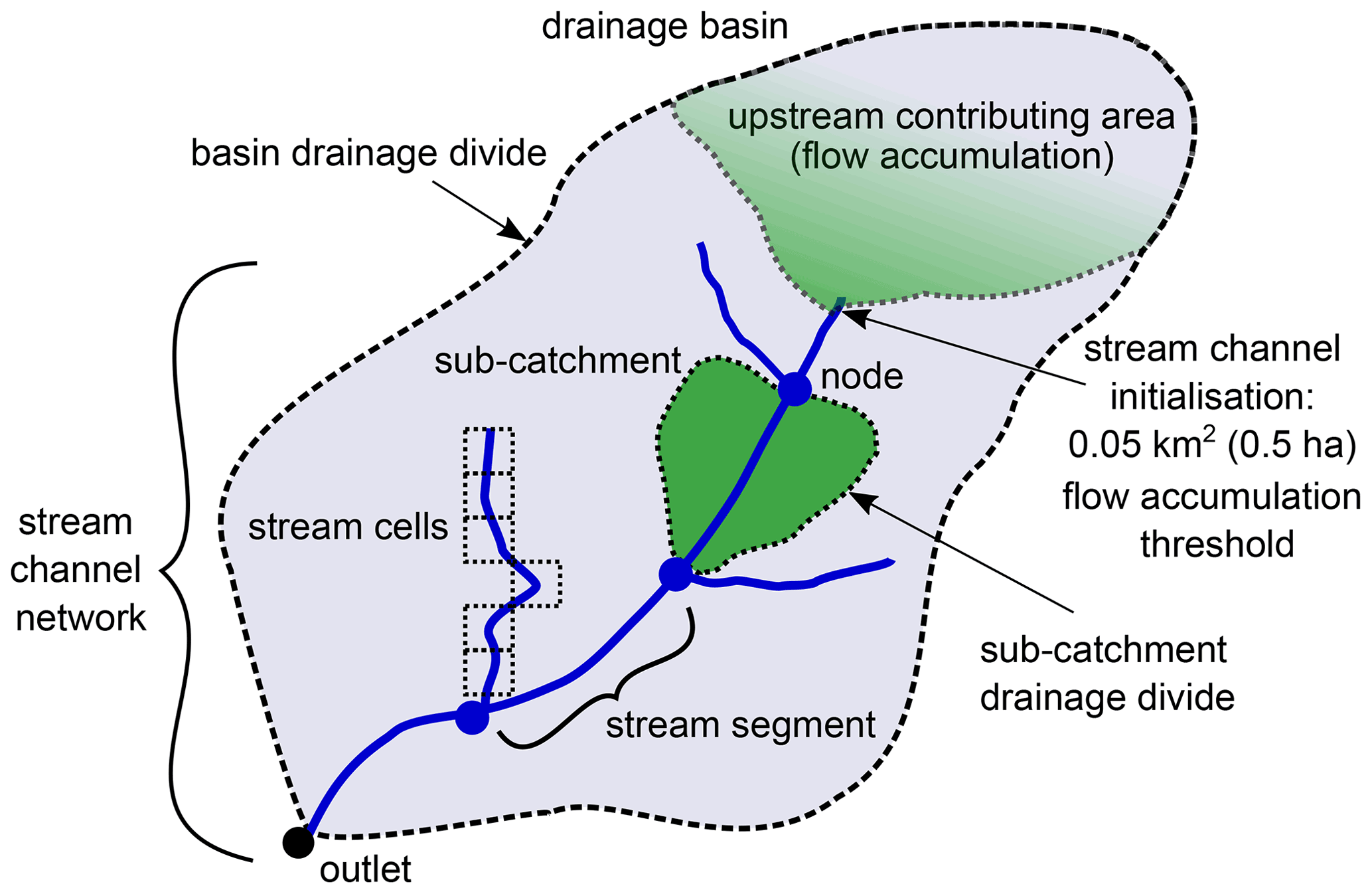
Figure 1 Schematic overview of the terminology used in Hydrography90m. See the main text for detailed descriptions.

2.2 Digital elevation model (DEM)

As the basis for all calculations, we used the MERIT Hydro DEM, which represents the best available globally seamless, high-resolution DEM to date (Yamazaki et al., 2019). The MERIT Hydro DEM is available for download at http://hydro.iis.u-tokyo.ac.jp/~yamadai/MERIT_Hydro/index.html (last access: 5 October 2022). In general, DEMs represent the elevated land surface in relation to a reference height such as sea level. In addition, DEMs are extensively deployed in geo-computational applications, as land surface plays a fundamental role in modulating earth-dynamic operations such as atmospheric, geomorphological, hydrological, and ecological processes. DEMs built from space-borne observations can achieve global coverage and thus have broad applications. However, the original space-borne DEMs are prone to systematic biases as well as random noise (Rodríguez et al., 2006; O'Loughlin et al., 2016). The systematic bias stems from the influence of tree canopies, while random noise can be classed into speckle, stripe noise, and absolute biases depending on their wavelengths (Rodríguez et al., 2006; Takaku et al., 2016). The Multi-Error-Removed Improved Terrain (MERIT) DEM (Yamazaki et al., 2017), at 3” resolution, extended from 90^∘ N to 60^∘ S, was the first global product with a consistent systematic bias and random noise removal procedure and is considered the best available seamless DEM with global coverage (Hirt, 2018; Moudrỳ et al., 2018). MERIT DEM is a fusion of the National Aeronautics and Space Administration's (NASA) SRTM3 version 2.1 (Farr et al., 2007), the Japan Aerospace Exploration Agency's (JAXA) AW3D global high resolution 3D map (version 1) (Tadono et al., 2015), and the Viewfinder Panorama’s DEM (available at http://www.viewfinderpanoramas.org/dem3.html, last access: 5 October 2022). The quality of MERIT DEM is unique, because it eliminates stripe noise using a 2-D Fourier filtering technique that is able to detect unrealistic regular terrain undulations. Absolute bias has been corrected by calculating the difference between the DEM and the ICESat elevations (Harding and Carabajal, 2005). Tree-height bias is addressed by combining tree density (Hansen et al., 2013) and tree height (Simard et al., 2011) and by comparing the obtained MERIT DEM to ICESat.

Even though the tree canopy bias was removed in MERIT DEM, the elevation information in grid cells with substantial tree coverage has a higher uncertainty compared to those without tree coverage (Yamazaki et al., 2017, 2019). Hence, the tree density map and G3WBM glacier map were used to enforce the separation of actual inland basins and dummy depressions by means of a correction of a predefined topographic volume that ascertains whether a depression is present or not (Yamazaki et al., 2017). Finally, speckle noise was removed using an adaptive-scale smoothing filter (Gallant and Wilson, 2000). Yamazaki et al. (2017) reported that, after the error removal, areas mapped with ±2 m or better vertical accuracy increased by 19 %, and slope distortions were reduced.

In 2019, Yamazaki et al. (2019) released the MERIT Hydro – a new global, hydrologically-adjusted DEM, which included depression, flow direction, flow accumulation, river width, and height above the nearest drainage (HAND) layers. The hydrologically adjusted elevation incorporates various surface water datasets (G1WBM Yamazaki et al., 2015; GSWO Pekel et al., 2016; and OpenStreetMap OpenStreetMap contributors, 2017) as well as a Landsat-derived tree density map (Hansen et al., 2013) and G3WBM glacier map to allow for an additional round of hydrological corrections (Yamazaki et al., 2015).

The water bodies serve as a carving template to modify the elevation of the MERIT DEM, satisfying the condition that “downstream is not higher than upstream” and to include valleys that are not depicted because they are smaller than the grid cells of the DEM (Yamazaki et al., 2019). The G1WBM and GSWO are Landsat-derived (30 m resolution) and therefore of limited use to depict tributaries smaller than 30 m river width or rivers with a width >30 m that are covered by tree canopy (Amatulli et al., 2020). On the other hand, OpenStreetMap (OpenStreetMap contributors, 2017) does depict small tributaries, depending on the region and the extent of survey efforts on the concerned water bodies. To date, not all countries in OpenStreetMap provide high spatial accuracy for headwater streams, and thus, headwater streams are not yet carved consistently into MERIT Hydro DEM (Amatulli, 2020; Amatulli et al., 2018a).

2.3 Flow routing algorithms

The flow accumulation operation performs a cumulative count of the number of grid cells (or other surface area units) that drain into outlets, given the terrain surface. Calculating flow accumulation involves three sequential algorithms: determining flow direction, addressing depressions and flat areas, and finally, calculating flow accumulation.

Several flow-routing algorithms exist for identifying streams channels at various spatial resolutions (Yang et al., 2010; Orlandini et al., 2003; Tarboton, 1997; Zhang et al., 2007b; O'Callaghan and Mark, 1984). They are built upon the observation that water follows the steepest route along a relief and accumulates in valleys, lowlands, flat areas, and depressions (Heine et al., 2004).

The most widely used algorithm is the single-flow (D8) (O'Callaghan and Mark, 1984) algorithm that assigns flow from a focal grid cell to only one of the eight neighbouring grid cells with the steepest slope. This algorithm accumulates, or pools, the entire flow from one cell to another, producing often distinct, artificially straight stream channels (Erskine et al., 2006), where the steepest gradient might lie between two of the eight directions (Seibert and McGlynn, 2007). D8 has been used to develop the HydroRIVERS (Lehner et al., 2008), the MERIT Hydro hydrography map (Yamazaki et al., 2019), and the MERIT Hydro–Vector dataset (Lin et al., 2021). Nonetheless, it is acknowledged that D8 algorithm is not adequate for representing flow contributing area in headwater regions (Yamazaki et al., 2019).

To overcome the limitation of the artificially straight stream channels (Erskine et al., 2006) of the D8, the multi-flow direction algorithm (MD8) has been proposed as an improvement. It splits the flow into multiple directions as a function of the slope in each of the neighbouring grid cells (Quinn et al., 1991, 1995) and produces stream channel patterns closer to reality than D8 does. In case of small elevation differences between two or more neighbouring grid cells, both cells receive about the same proportion of the accumulated area. The disadvantage of MD8, as presented by Quinn et al. (1991), is that the area from one grid cell is routed to all downslope grid cells without considering a divergence or convergence hillslope factor, which would increase or decrease the dispersion rate as a function of the tangential curvature. To minimise this problem, Holmgren (1994) suggested partitioning the flow according to a convergence factor ranging from 1 to 10 (suggested value 5).

This MD8 is defined as

$$fi={\displaystyle \frac{(\tan {\mathit{\beta }}_i{)}^x}{\sum (\tan {\mathit{\beta }}_i{)}^x}},$$

where β is the slope gradient and x is a weighting factor. The MD8 algorithm, as opposed to D8, is better able to handle a wider range of terrain, including flat areas where flow routing is challenging (Liang and MaCkay, 2000). It therefore allows the extraction of stream channels of headwaters and small, non-perennial streams in greater detail than D8 does.

Alternatively, Tarboton (1997) has suggested the use of triangular facets to overtake the eight possible directions of the D8. Tarboton (1997) named this method D∞, which describes the infinite behaviour of the dispersion of the single-direction flow pathways. Nevertheless, we opted for MD8 using the traditional Holmgren method, which has been implemented in GRASS GIS (named “FD8”) (Neteler et al., 2012; Neteler and Mitasova, 2013) within several hydrological modules and which shows similar performance to the D∞ (Seibert and McGlynn, 2007) in hydrologically and algorithmically challenging terrain, such as flat areas (Jasiewicz and Metz, 2011).

2.4 Depression and endorheic basins

We overlaid the depression layer from MERIT Hydro (Yamazaki et al., 2019) with the HydroLAKES dataset (Messager et al., 2016) and identified 1400 interior lakes that coincide with depression points that mark inland depressions. We then rasterised these lakes to the 3×3 arcsec grid cell resolution and, together with the MERIT Hydro depression layer, we assigned these areas as NoData in MERIT Hydro (i.e. no outflow from these lakes). Such a procedure was needed, for instance, to treat the Caspian Sea, an inland depression, to route the flow accumulation correctly until the coast line. This procedure also created many small, surrounding drainage basins only connected to lakes. In addition, we assigned the geographic locations (i.e. the single 3×3 arcsec grid cells) of all remaining depression points in MERIT Hydro as NoData.

2.5 Computational stages

The overall computation of the Hydrography90m consisted of four stages:

• splitting the global DEM into smaller spatial units (tiles) to achieve computational scalability;

• computing flow accumulation and direction, and the subsequent extraction of stream channels and basins;

• validating the spatial distribution of stream channels and basins using independent data sources;

• computing geophysical, morphological, and topological properties of the stream channels and basins.

Several procedures within the entire workflow were repeated at different stages, including the use of intermediate layers from preceding stages in the creation of final layers. The entire work flow was automated with Bash scripts to integrate a hybrid operation of multiple open-source software. These procedures were run at the High Performance Computing (HPC) facility of the Center for Research Computing, Yale University:

• Geospatial Data Abstraction Library (GDAL), version number 3.1.0 (GDAL Development Team, 2020): for tiling, cropping, mosaicking, merging, and image compression

• Processing Kernel for geospatial data (Pktools), version number 2.6.7.6 (Kempeneers, 2018; McInerney and Kempeneers, 2015): for masking, creating histograms, and re-classification analyses

• Geographic Resources Analysis Support System – Geographic Information System (GRASS GIS) software, version number 7.8.0 (GRASS Development Team, 2019): for computing the hydrography.

These tools provided fast, flexible, and scalable features and functions for raster-based analysis with Python APIs and Bash command access (Amatulli et al., 2014). They also enabled multi-core parallel processing of very large datasets owing to efficient algorithms and optimised memory management. The entire workflow consisted of eight main tasks (labelled with letters in Fig. 4), for which we used a total of three GRASS GIS modules and several GIS commands (i.e. cropping, re-class, merging, etc.) and yielded both intermediate and final outputs within the given tiling system.

3 Tiling the DEM

3.1 Irregular tiling system (ITS)

To address the high computational demand for calculating flow accumulation at 3×3 arcsec resolution globally, we split the entire MERIT Hydro DEM into 59 tiles of varied sizes to yield an irregular tiling system (ITS, red squares in Fig. 2). These irregular tiles were large enough to contain one or more entire drainage basins, such that their lateral and longitudinal connectivity is maintained within each tile. For an initial approximation of the location and size of the basins and, hence, the position of the tiles, we aggregated MERIT Hydro from 3×3 to a 30×30 arcsec resolution while preserving the minimal value of elevation in each cell. The resulting global DEM matrix of 751 680 000 grid cells at 30×30 arcsec resolution allowed us to compute drainage basins on a global scale using the GRASS GIS module r.stream.basins. We then manually created rectangular tiles considering (i) the maximum possible number of ∼2 billion grid cells (2³1−1, that requires ∼67 GB of RAM) within a tile, and (ii) that large drainage basins were completely within a given tile, while (iii) keeping a buffer of 1^∘ longitude and latitude. The tiles naturally overlap with each other because of the irregular shapes of adjacent drainage basins. By merging all entire drainage basins within the 59 irregular tiles, we obtained a representation of the world's drainage basins at 3×3 arcsec resolution (Fig. 2).

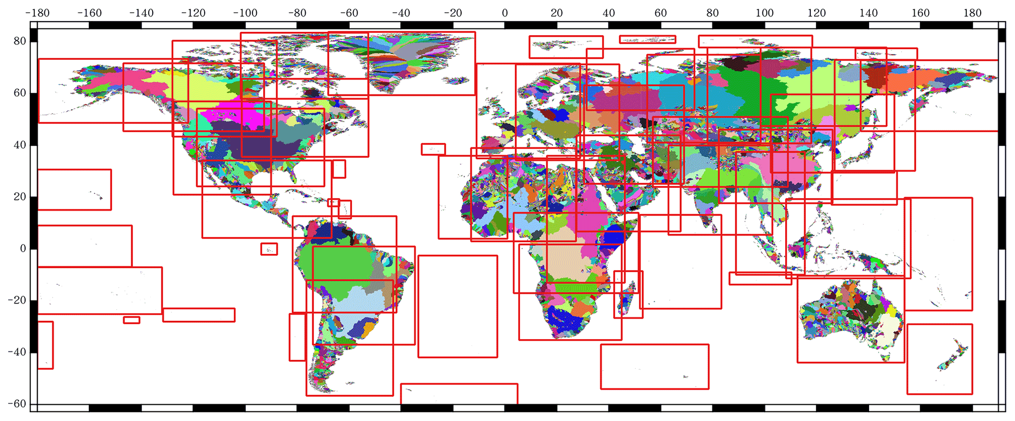
Figure 2 The irregular tiling system (ITS, in red) overlaid with the global drainage basins at 3×3 arcsec resolution (random colours for illustrative purposes). Within a tile, we retain only the areas that belong to entire drainage basins, so as to preserve lateral and longitudinal connectivity within the basin.

3.2 Regular tiling system (RTS)

In addition to the ITS, we also built a regular tiling system (RTS) consisting of 116 tiles with a fixed dimension of 20^∘longitude $\times {\mathrm{20}}^{\circ }$ latitude (ranging from −180 to $+{\mathrm{191}}^{\circ }$ longitude and from +85 to $-{\mathrm{60}}^{\circ }$ latitude). This RTS was implemented to avoid the handling and distribution of a single and computationally heavy global file. We modified the size of two eastern tiles, since the traditional map view of MERIT Hydro splits drainage basins at −180 and $+{\mathrm{180}}^{\circ }$. We set the Bering Strait as the border of the map in the north-east, where the tiles reached $\mathrm{31}{}^{\circ }\text{longitude}\times {\mathrm{20}}^{\circ }$ latitude (i.e. the eastern boundary was expanded to 191^∘to include the Chukotka region in Russia). We repeated this for southern tiles, reaching $\mathrm{20}{}^{\circ }\text{longitude}\times {\mathrm{25}}^{\circ }$ latitude (i.e. the southern boundary was expanded to $-{\mathrm{60}}^{\circ }$ latitude to include southern islands). All distributed Hydrography90m raster and vector files are available for download in tiles. The tile labels are reported in Fig. 3. In case the area of interest crosses several tiles, the data needs to be merged to combine the cross-border drainage basins. We provide easy-to-use, efficient code and instructions to merge the tiles for vector or raster files at http://hydrography.org (last access: 5 October 2022). No border effects or artefacts remain after the merge.

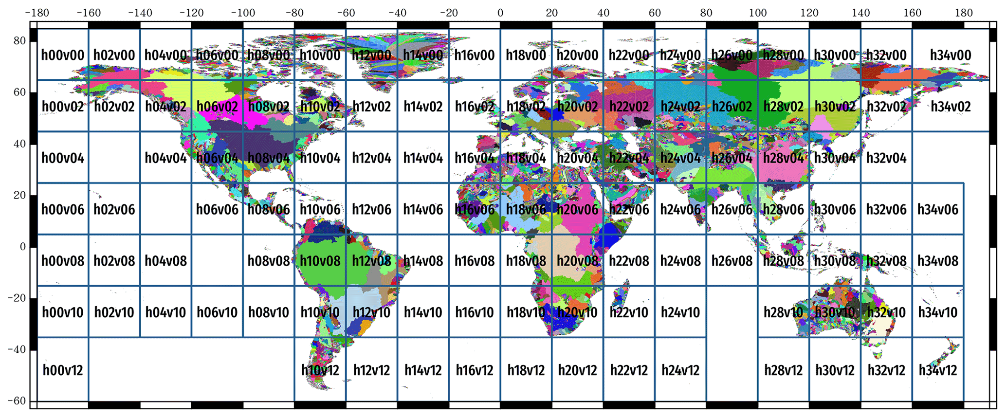
Figure 3 The regular tiling system (RTS, in blue) overlaid with global drainage basins at 3×3 arcsec resolution (random colours for illustrative purposes). Tile labels correspond to the names of raster and vector data available for download, which are listed in Tables 1, 3, 4, 5, 6, 7. We provide an interactive map at http://hydrography.org (last access: 5 October 2022) that allows clicking on a given tile to directly download the data.

4 Computing the base and network hydrographic layers

The stream channel extraction and the drainage basin delineation were performed in GRASS GIS software using the r.watershed (Metz et al., 2011) module, followed by r.stream.extract (Jasiewicz and Metz, 2011) as well as the r.stream.basins (Jasiewicz and Metz, 2011) module, respectively. The work was split into two phases (Fig. 4): the first phase produced a globally seamless representation of the flow accumulation, whereas the second phase generated the stream channels and associated data.

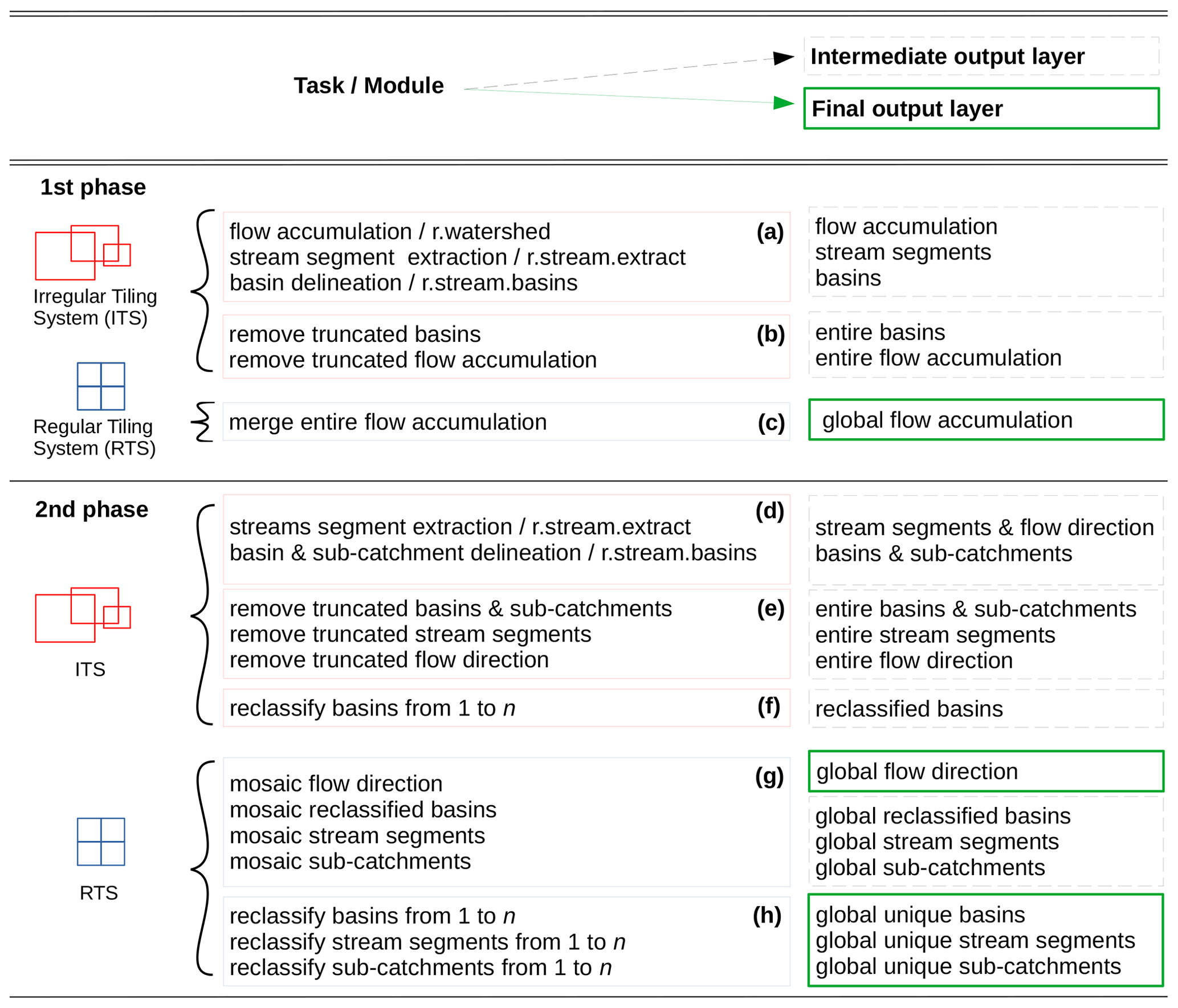
Figure 4 Overview of the Hydrography90m dataset computation workflow. Task labels correspond to the performed computation, and command labels refer to the GRASS GIS module used. The parenthesised letters listed in the figure correspond to steps detailed in the methodology section. A schematic scripting procedure of the workflow for three South American tiles is reported at http://hydrography.org (last access: 5 October 2022). The scripting procedure is related to the first and second phases but without the final reclassification step to have a simplified workflow example.

4.1 Flow accumulation within the irregular tiling system (ITS)

For each irregular tile, we ran the r.watershed module to produce a flow accumulation map (one for each tile) based on the MD8 multi-flow direction algorithm (Holmgren, 1994). In r.watershed, we used the MERIT Hydro elevation and depression layers as inputs in addition to a “surface area in km²” layer at 3×3 arcsec resolution for downstream area accumulation. The latter provides the surface area expressed in km² within each 3×3 arcsec grid cell. This was necessary, as we computed the hydrography in the unprojected WGS84 coordinate reference system (Fig. 4a).

4.2 Checking for truncated drainage basins (ITS)

Each irregular tile included the flow accumulation as well as the drainage basins and stream channels within the circumscribed drainage basins. Some drainage basins were entirely hemmed within a given tile, while others were partially included because they spread across multiple tiles (and where the tile could not be enlarged beyond the maximum number of grid cells). These partially included or truncated basins were identified (and removed) by querying for those that intersected a tile border. This left only entire drainage basins and the associated flow accumulation (Fig. 4b).

4.3 Merging the global flow accumulation

We merged the 59 irregular flow accumulation tiles, which yielded the 116 smaller tiles of the RTS (ranging in size from a few MB to 2 GB, stored as Float32 data type), to a globally seamless flow accumulation layer at 3×3 arcsec spatial resolution (Fig. 4c). This was done in the interest of producing manageable file sizes.

The creation of this 3×3 arcsec resolution, globally seamless flow accumulation layer, computed with the MD8 algorithm, can be considered a pioneering computational achievement. It serves as the foundation for Hydrography90m and, to our understanding, will allow for significant expediency in the future computation of any derivative hydrological products.

4.4 Stream channel and basin delineation computation (ITS)

We used the seamless global flow accumulation to re-compute the drainage basins, flow direction, and stream network. This resolved any errors that could have occurred at the tile borders and truncated drainage basins, given possible rounding errors in the grid cell alignment when cropping drainage basins at 3×3 arcsec resolution at a global extent. Again, we ran r.stream.extract followed by r.stream.basins, masking all previously identified truncated drainage basins (Fig. 4d, e).

4.5 Mosaic drainage basins, sub-catchments, streams segments, and flow direction

In each tile in the ITS, several drainage basins were computed, having a unique identifier (ID) ranging from 1 to n ID. Prior to creating the global mosaic, we reclassified all drainage basin IDs from 1 to n in order to consecutively number the basins across the globe (Fig. 4f). We repeated this re-classification after the global merging to ensure that the ID series from 1 to n was continuous and thereby avoided any gaps in the ID sequence. Ultimately, the re-classification yielded a total of 1 560 490 globally unique drainage basin IDs. A similar reclassification procedure was performed on the sub-catchment and stream segment IDs (Fig. 4g, h).

A global representation of the network hydrography layers produced with such methodology is shown in Fig. 5. A more detailed representation is depicted in Fig. 6 and the corresponding Table 1. The table lists the file description and GRASS GIS commands for locating these layers in the data repository and reproducing the calculations (Table 1). Additional features of the layers are available in the relevant GRASS GIS module manual pages.

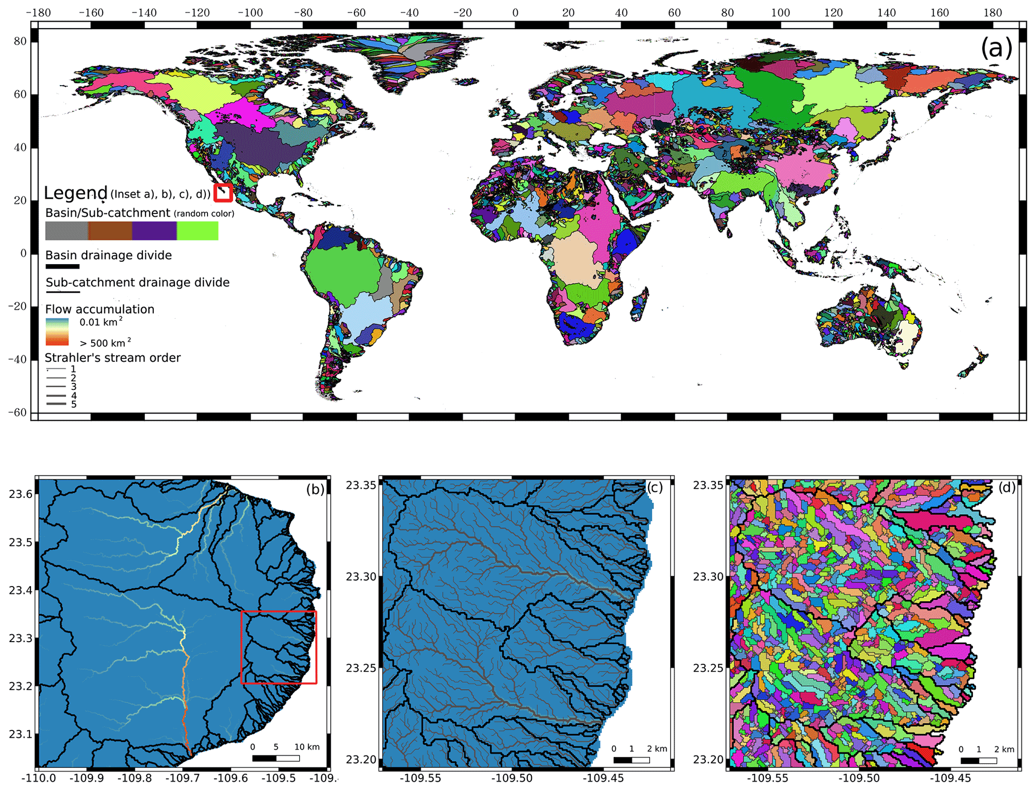
Figure 5 Map (a) shows the global distribution of the newly delineated 1.6 million drainage basins. The red box in Baja California Sur, Mexico, represents the location of inset (b). This inset shows flow accumulation and the basin drainage divide. Inset (c) shows flow accumulation and the stream channel network, where line width corresponds to the Strahler stream order. Map (d) illustrates the corresponding sub-catchments, sharing an identifier ID with stream channels. Drainage basin and sub-catchment colour assignment is random and for illustrative purposes only.

Table 1 Base and network layers of Hydrography90m: flow accumulation, flow direction, drainage basins, outlets, stream segments, sub-catchments, regional units, and depression; Map reference corresponding to Fig. 6 for raster visualisation and Fig. 5 for vector visualisation; Unit; Commands for computation; and Output file names. The asterisk stands for the regular tile ID for downloading the data, available in ${\mathrm{20}}^{\circ }\times {\mathrm{20}}^{\circ }$ tiles (Fig. 3).

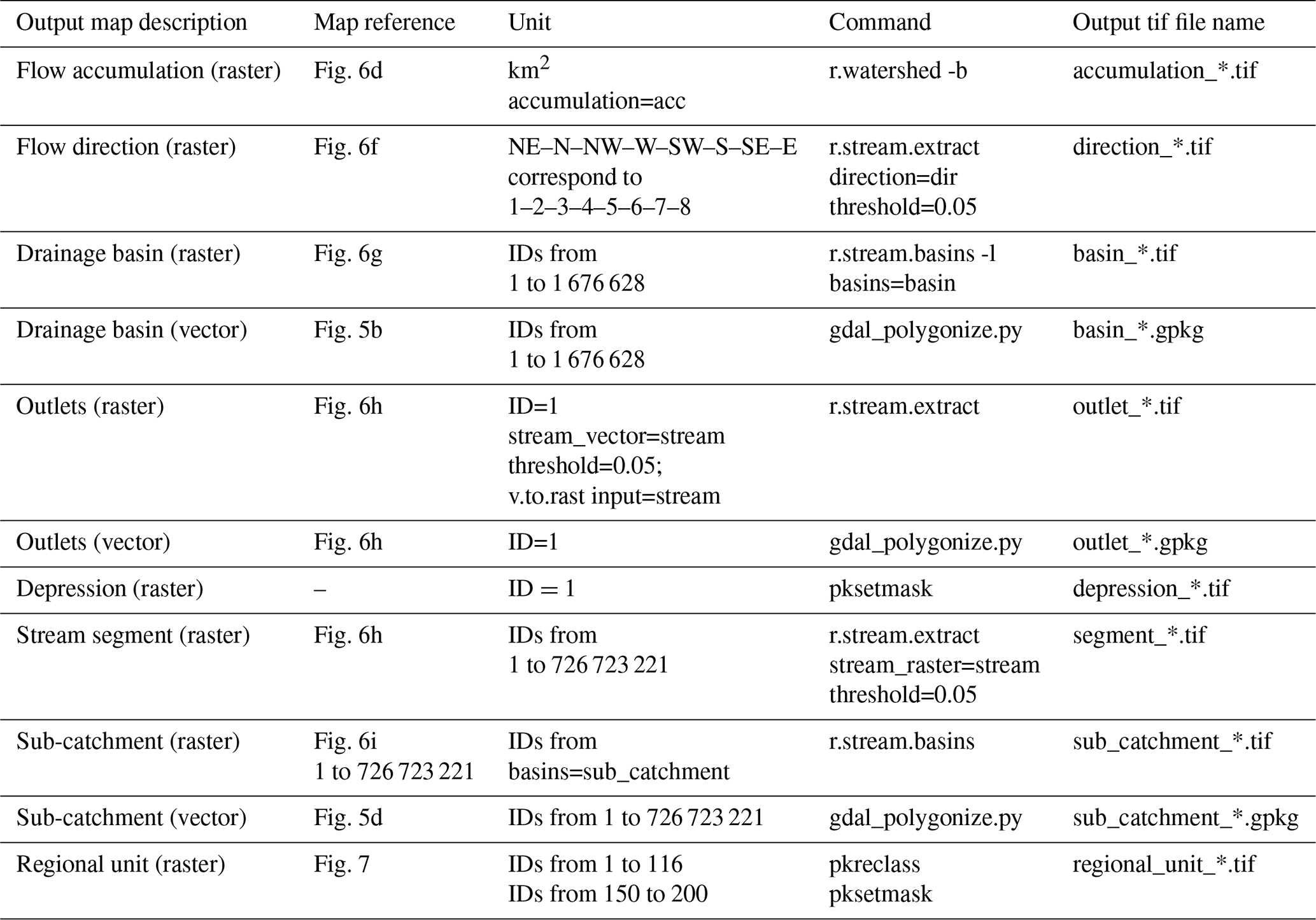
Figure 6 Map (a) shows the MERIT Hydro DEM for an area of 13×11 km in north-west Italy, and (b–i) show the base and network layers of Hydrography90m. The sea is depicted in dark grey. The outlets are shown in panel (h) as red points.

4.6 Regional units

In addition to the base hydrography layers, we provide a “regional unit” raster map that holds 166 regional unit IDs and that contains only entire drainage basins. Such units are useful for splitting whole global hydrography layers into single drainage basins or other units of manageable size. Each regional unit, together with the correspondent Hydrography90m layers, can be loaded into GRASS GIS for additional computation, accounting for less than ∼2 billion grid cells. Such regional units are meant only to address computational requirements and are not for the consideration of any eco-region context or hydrological similarity. Here, the 50 largest drainage basins, such as the Nile, Amazon, or Mississippi drainages, correspond to 50 single regional units, and the remaining 116 regional units include two or more smaller entire drainage basins. A global representation of the 166 regional units is shown in Fig. 7. The details for regional unit IDs are provided in the last row of Table 1. In case users want to perform a hydrological analysis within each single “regional unit”, they may first need to merge the data across tiles and then identify and mask the specific “regional unit” of interest. We provide easy-to-use, efficient code and instructions at http://hydrography.org (last access: 5 October 2022).

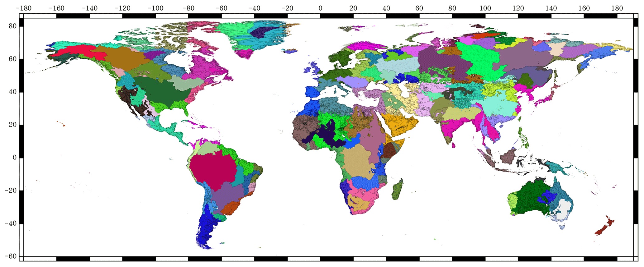
Figure 7 The 166 regional units that facilitate the splitting of all the Hydrography90m layers into customisable zones, including those areas that are delimited by an entire basin. The first 116 regional units (IDs 1 to 116) include two or more entire drainage basins, e.g. the green regional unit in the north of Europe, which includes several such basins. The remaining 50 units (IDs 150 to 200) each contain one of the 50 largest drainage basins in the world, e.g. Nile basin, Amazon basin. The colour assignment is random and for illustrative purposes only. Each coloured unit holds an ID at 3×3 arcsec grid cell resolution and serves to mask any neighbouring drainage basins that may not be within a given area of interest (see usage notes for more details).

5 Validation of the Hydrography90m

We validated the accuracy of the stream channels spatial position and the flow accumulation against the independent and observed NHDPlus HR vector dataset (Moore et al., 2019) of the United States.

5.1 Spatial accuracy of the streams

We then compared the newly delineated Hydrography90m against three other global datasets: the HydroRIVERS dataset (Lehner et al., 2008), the Global River Widths from Landsat (GRWL, Simplified Vector Product V01.01) (Allen et al., 2018), and the MERIT Hydro–Vector hydrography dataset (Lin et al., 2019). These vector-based datasets were brought to a 3×3 arcsec grid cell resolution using gdal_rasterize to allow a direct comparison with the newly-developed Hydrography90m stream network dataset.

Since none of these previous products had delineated headwater streams at a high spatial precision, we used the NHDPlus HR vector dataset as a reference to compare the accuracy of our newly delineated stream channels. The NHDPlus HR is built based on the National Hydrography Dataset High Resolution data (1:24 000 scale), 3D Elevation Program data (10 m resolution), and the Watershed Boundary Dataset (1:24 000 scale) (Buto and Anderson, 2020). We likewise rasterised the NHDPlus HR vector lines to a 3×3 arcsec grid cell resolution to allow for a direct comparison. We then buffered the NHDPlus HR gridded stream lines in five categories, the first category (buffer-0) being the grid cells where the NHDplus HR network overlaps, and the other four categories (from buffer-1 to buffer-4) representing 100 m interval buffers (Fig. 8). We overlaid the four datasets with each of the buffered ranges and calculated the number of overlapping grid cells in each dataset within the given buffer distance. This procedure accounted for the lateral accuracy of each hydrographic dataset when compared to the NHDPlus HR reference dataset. In addition, in order to estimate stream length, we quantified the length of each stream channel as the number of stream grid cells relative to the length of the NHDPlus HR streams.

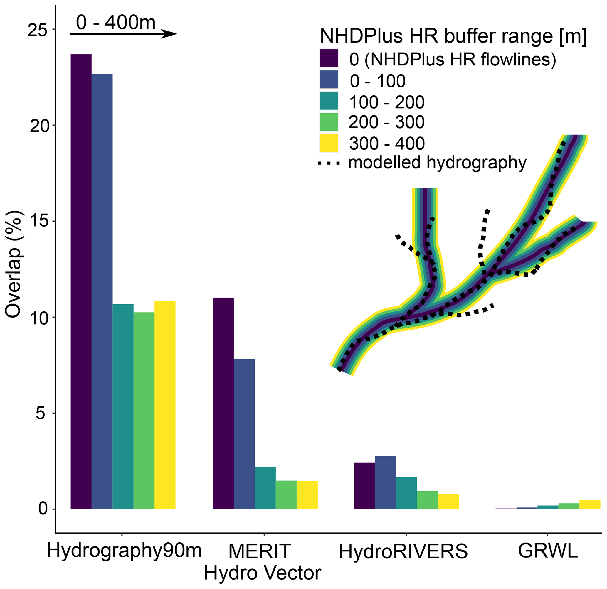
Figure 8 Comparison of the spatial accuracy of the newly developed Hydrography90m and the MERIT Hydro-Vector, HydroRIVERS, and GRWL datasets against NHDPlus HR. The inset shows the validation method: we first buffered NHDPlus HR by 100, 200, 300, and 400 m (see corresponding colours) and then calculated the fraction of overlapping stream grid cells between NHDPlus HR and each dataset. The latter are illustrated here as dotted lines.

The validation showed that the Hydrography90m has the highest lateral accuracy within the smallest buffer ranges among each of the compared dataset pairs (Figs. 8, 9). Within a buffer distance of 100 m, Hydrography90m overlaps with NHDPlus HR by 46 %, achieving the highest overlap among all available global hydrographic datasets (Fig. 8). Assessing the proportion of stream channels in each hydrography dataset versus NHDPlus HR showed that Hydrography90m underestimated the total river length, with 28 % fewer stream grid cells than NHDPlus HR. In comparison, the MERIT Hydro-Vector contained 77 %, the HydroRIVERS 92 %, and the GRWL 99 % fewer stream grid cells than the NHDPlus HR (Fig. 9). This discrepancy in overall stream length and coverage among the different hydrographies is also shown in Fig. 9. Hydrography90m hence provided an all-inclusive approach by also considering potential stream channels contingent on water availability, delineating small headwater streams for the first time globally, and providing an important baseline for the future assessment of stream flow within these channels.

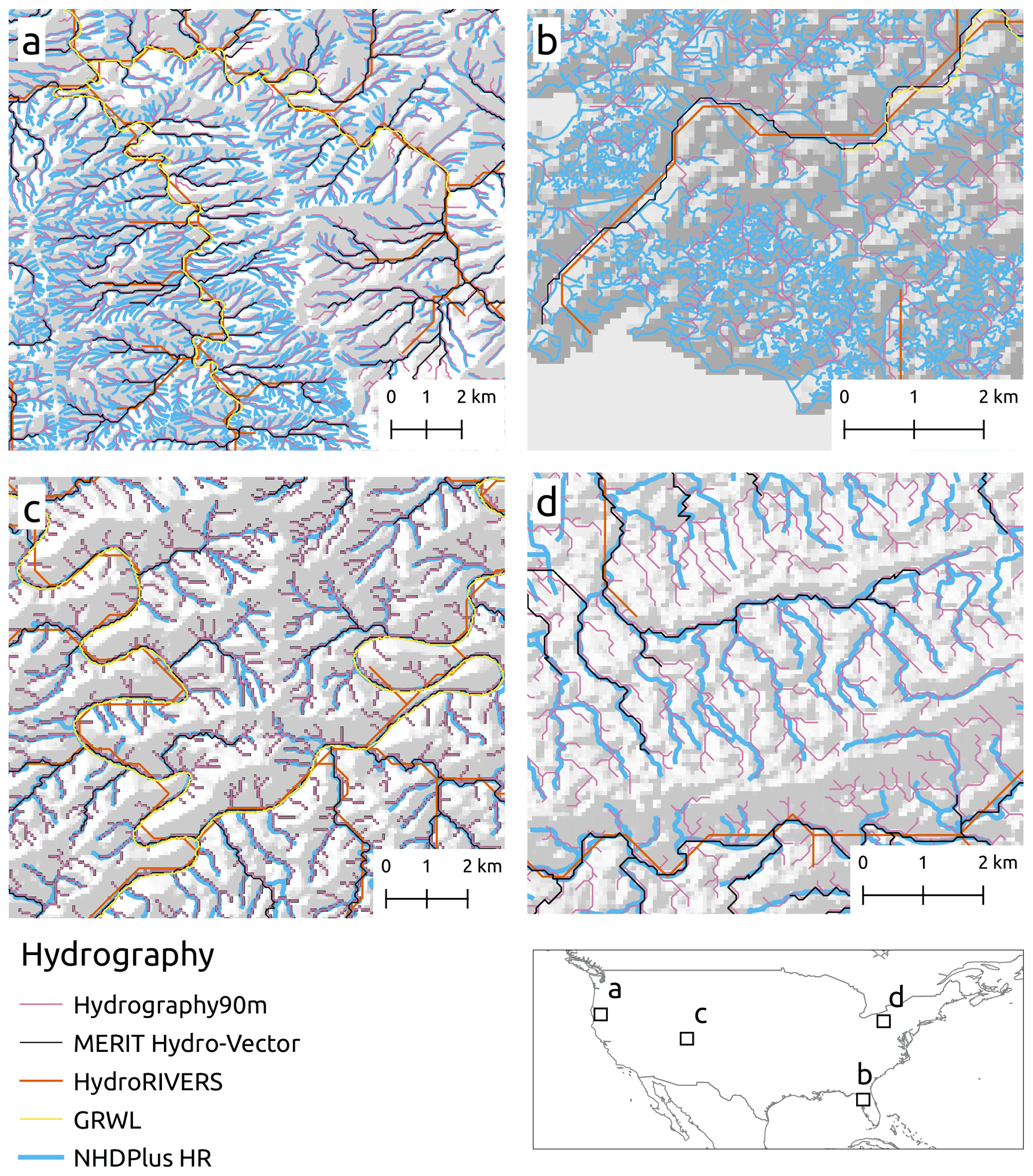
Figure 9 Visualisation of the different global hydrographic datasets (Hydrography90m, MERIT Hydro-Vector, HydroRIVERS, GRWL) against the high-resolution NHDPlus HR reference dataset of the United States (Buto and Anderson, 2020). The geographic location of the four panels (a)–(d) corresponds to the labels in the map.

5.2 Flow accumulation accuracy

The NHDPlus HR vector dataset attribute table reports the flow accumulation for each stream segment. The flow accumulation was computed using a 10×10 m 3D Elevation Program (3DEP) (Sugarbaker et al., 2014) DEM. The high resolution of 3DEP allows for precise flow routing and flow accumulation, which can then be used to validate the Hydrography90m flow accumulation. The flow accumulation values are reported in the NHDPlus HR vector attributes, labelled as TotDASqKm. We rasterised these stream segment TotDASqKm attributes to a 3×3 arcsec grid cell resolution using gdal_rasterize. The rasterisation process was performed using the maximum value of the TotDASqKm flow accumulation as standard, in case more than one stream segment fell within the same grid cell. We did not include all the streams that appear inside lakes, due to the emergence of the “fish-bone” structure (Domisch et al., 2015a), which depicted stream channels as artificial straight lines due to zero slope. We masked such features using the HydroLAKES dataset (Messager et al., 2016).

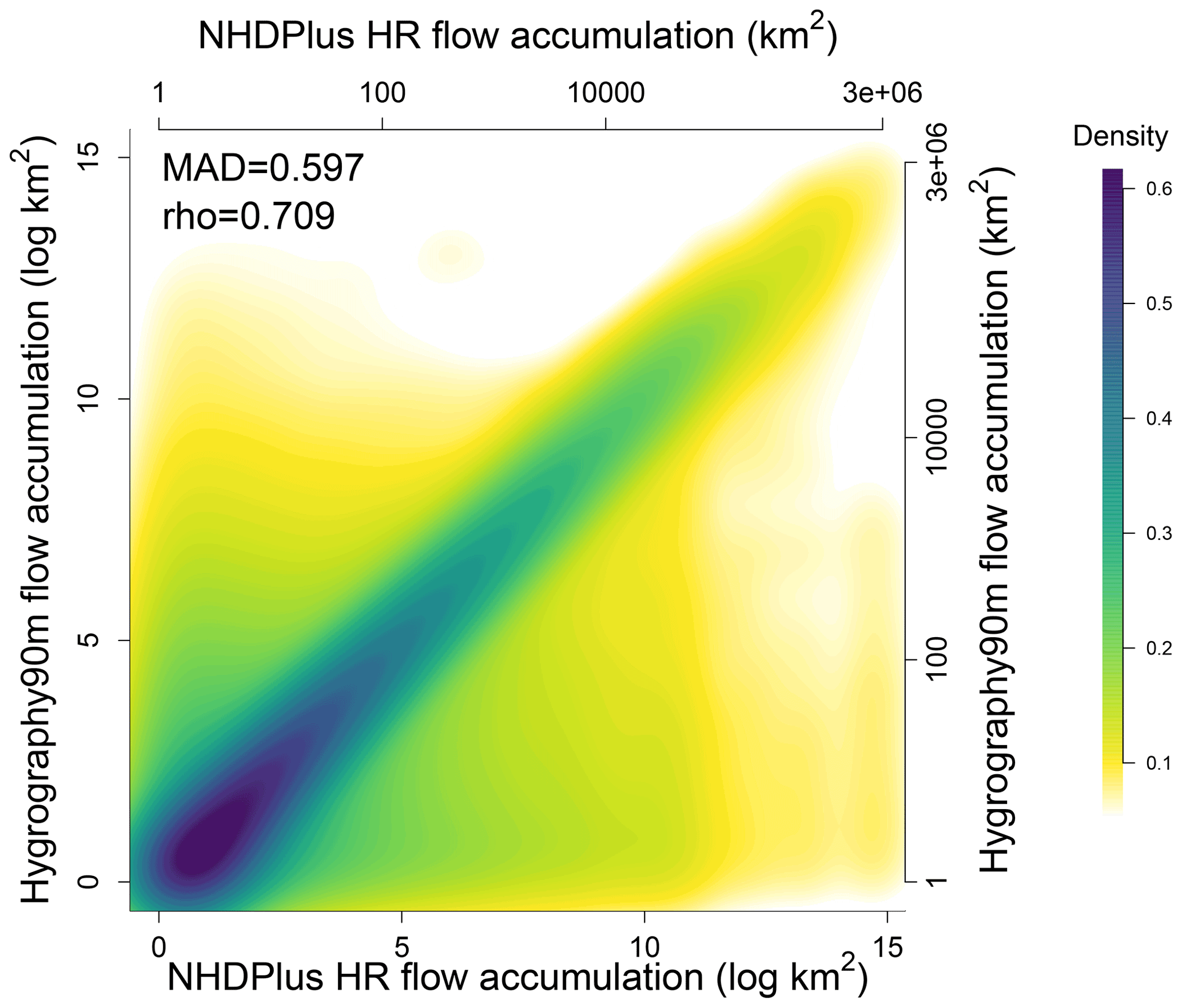
Figure 10 Density plot of Hydrography90m vs. NHDPlus HR flow accumulation (log-scale) of those 28 million stream channel grid cells with a flow accumulation larger than 1 km². Median absolute deviation (MAD) and Spearman coefficient (rho) were computed using all 61 million stream channel grid cells. The colour bar indicates a 2D kernel density estimate.

For statistical accuracy, we then selected those rasterised NHDPlus HR streams that overlapped with the Hydrography90m stream channels and, hence, extracted the Hydrography90m flow accumulation. A total of 61 million grid cell values were used in this procedure to compute the median absolute deviation (MAD) and Spearman coefficient (rho). These values are depicted in the 2D kernel density scatter plot in Fig. 10.

In addition to the NHDPlus HR flow accumulation comparison, we compared the surface areas of the 10 largest drainage basins worldwide (Table 2) among the HydroBASINS level 3 (Lehner and Grill, 2013) and HYDRO1k (USGS EROS Archive, 2018) datasets. These 10 basins drain a substantial amount of 31.5 % of the world’s land surface (Table 2), and the comparison showed, in general, a high agreement in the basin surface area among the datasets.

Table 2 The surface area of the 10 largest drainage basins worldwide in km², compared among the Hydrogryphy90m, HydroBASINS (Lehner and Grill, 2013), and Hydro1k (USGS EROS Archive, 2018) datasets.

6 Stream topographic and topological variables

In addition to the base hydrography layers (flow direction and flow accumulation) and network layers (drainage basins, stream channels, and sub-catchments), we produced layers that characterise the topographic and topological properties of the hydrography. These variables were computed along stream channels, e.g. stream slope, or across continuous land surfaces, e.g. distance to the stream.

6.1 Stream slope

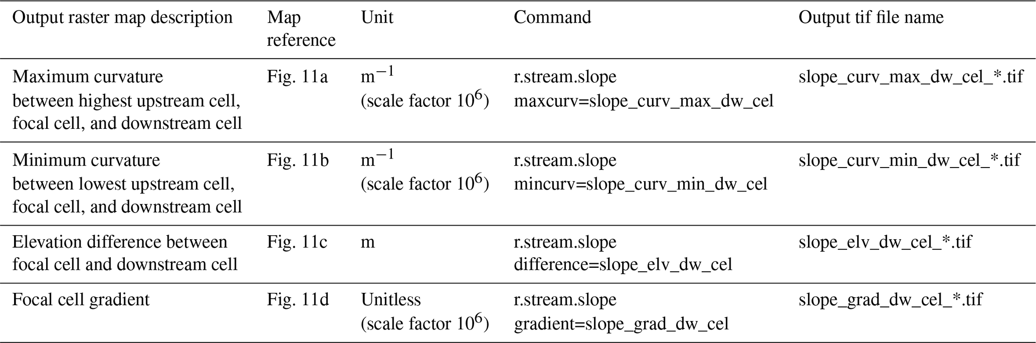
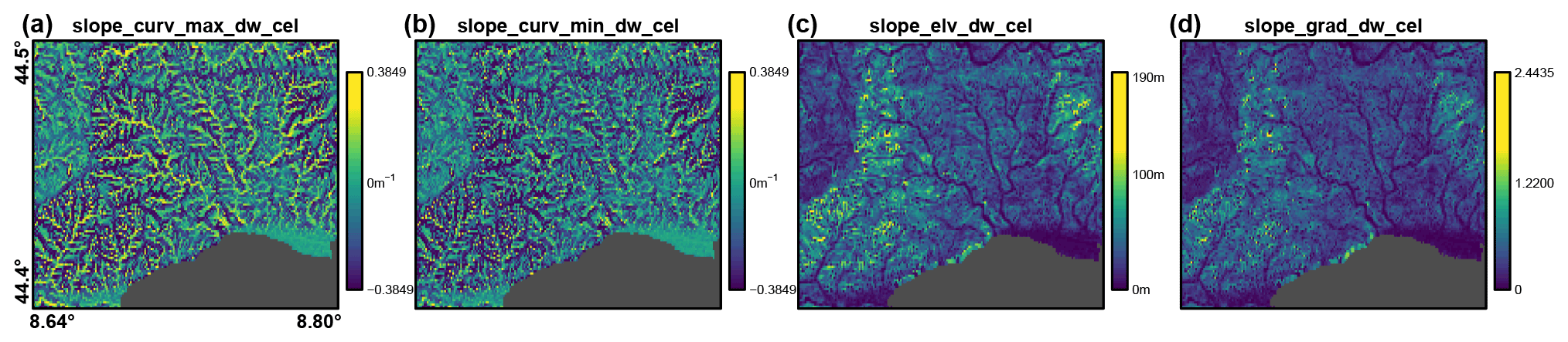
We calculated various stream channel slope properties at 3×3 arcsec stream grid cell resolution (as opposed to segment level), (Fig. 1), including minimum and maximum curvatures, gradient (slope), and elevation differences across the hydrography using the r.stream.slope (Jasiewicz and Metz, 2011) GRASS GIS module. Stream slope metrics were calculated between the current cell and the adjacent downstream and upstream cell. Stream channel properties, such as curvature, can be important for estimating channel bank shear stress and channel evolution (Buraas et al., 2014), whereas stream slope can be used in ecological studies as an indirect indicator of flow velocity and gas transfer velocities (Raymond et al., 2012; Kuemmerlen et al., 2014). All stream slope variables play a role in in-stream sediment transport (Yang, 1977) and the calculation of hydraulic flow and stream power (Hankin et al., 2019).

Table 3 Curvature, gradient (elevation difference divided by distance), and elevation difference raster maps computed with the r.stream.slope GRASS GIS module; map reference corresponding to Fig. 11; specific GRASS GIS command; and output layer name.

Figure 11 Maps (a)–(b) show curvature and gradient (elevation difference divided by distance) attributes of each land grid cell to the closest cell along the stream channel, computed using the r.stream.slope GRASS GIS module. The panel letters correspond to those in Table 3.

6.2 Stream distance

We calculated various distance metrics by setting the (i) stream channels, (ii) outlets, or (iii) stream nodes as starting points, using the r.stream.distance (Jasiewicz and Metz, 2011) GRASS GIS module. These metrics were based on the distance to (or elevation difference between) the shortest (nearest) or longest (farthest) paths calculated along the upstream and downstream directions. In the case of upstream direction, the shortest or longest paths are given by the MD8 algorithm, which distributes flow accumulation to multiple grid cells. Therefore, the nearest path is considered the shortest trajectory that the largest quantity of water follows from a given stream and/or focal cell to the drainage divide, while the farthest one represents the longest possible path and is the one that receives less water. Instead, for the downstream direction, water always follows the shortest path going from divide to stream.

These metrics are important for estimating the peak-to-valley time-lag effects of water flow and can aid in the prediction of travel time. The stream or outlet distance raster files are listed in Table 4. Both Euclidean (“as-the-crow-flies”) and dendritic (“as-the-fish-swims”) stream distance metrics along the network are widely implemented in spatial species distribution modelling, with the latter metric being more effective in modelling the dispersal of aquatic organisms (Mozzaquattro et al., 2020; Altermatt, 2013; Grant et al., 2007). Moreover, stream distance metrics are essential for calculating sediment delivery ratios (Walling, 1983).

Table 4 Stream or outlet distance and elevation difference raster maps computed with the r.stream.distance GRASS GIS module; map reference corresponding to Fig. 12; unit; GRASS GIS command; and output layer name.

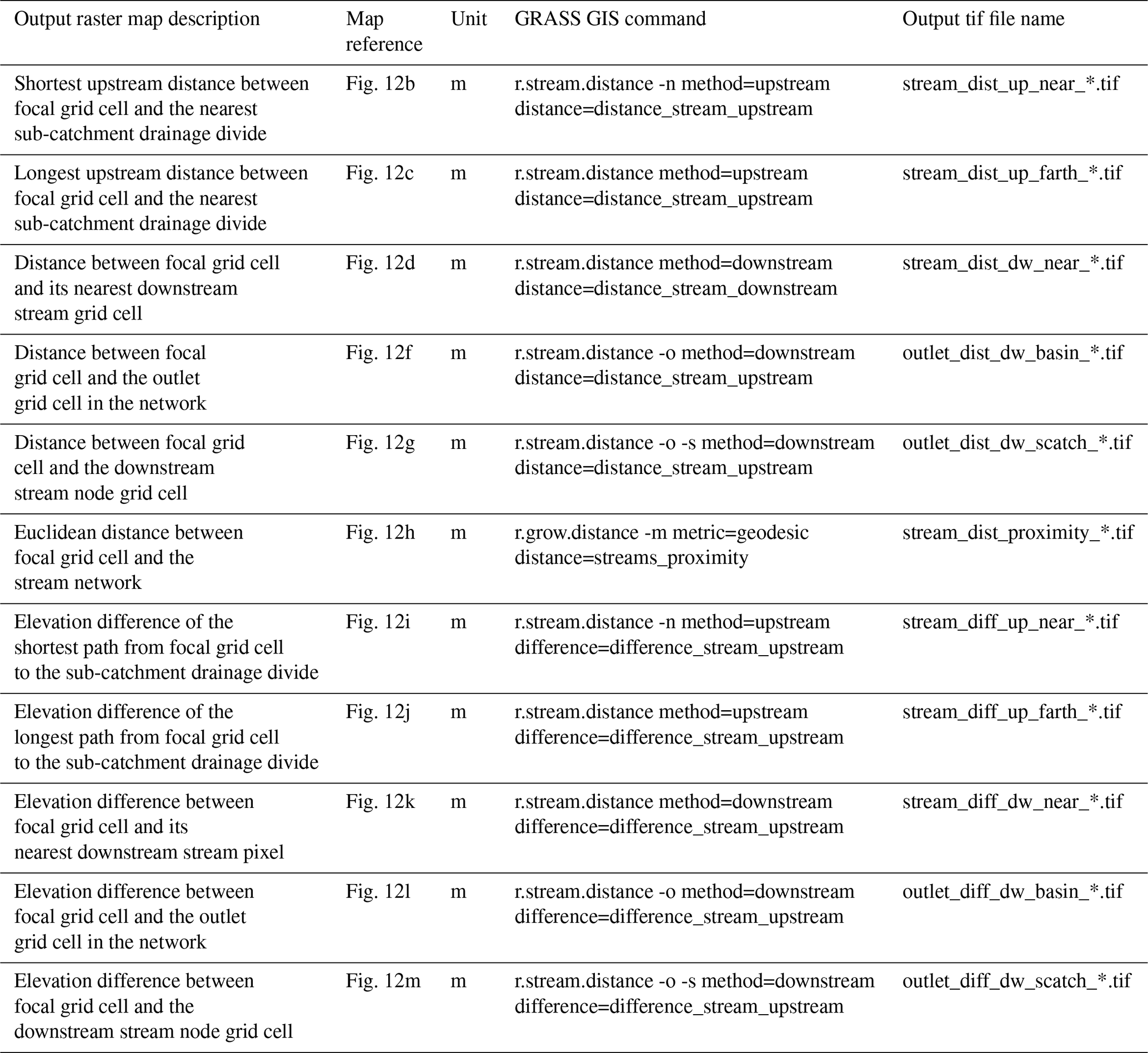
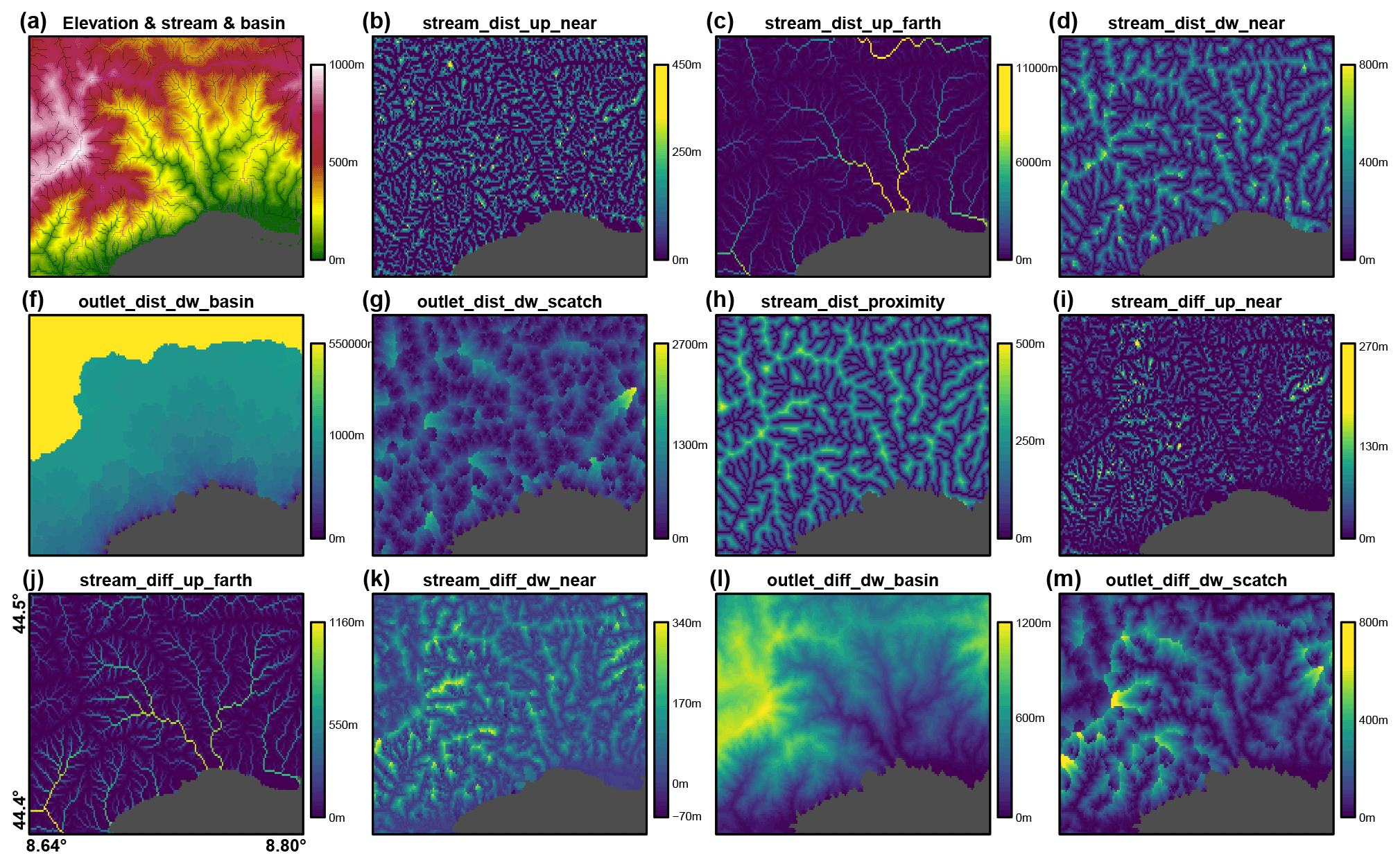
Figure 12 Map (a) shows the stream channels and drainage basins derived from the elevation layer. Maps (b)–(m) show, for the same area, the distance and elevation difference attributes of each land grid cell to the stream channels, outlets, or stream nodes using the r.stream.distance GRASS GIS module. The panel letters correspond to those in Table 4.

6.3 Stream segment properties

We calculated segment properties of the stream channels (as opposed to calculating within individual grid cells) (Fig. 1) across the hydrography – including the up- or downstream elevation difference, gradient (elevation difference divided by distance), and curvature within each stream segment – using the r.stream.channel (Jasiewicz and Metz, 2011) GRASS GIS module. The segment properties of the stream channels were calculated downstream for every segment, from its initialisation to the outlet or node or from a focal cell to the outlet or node (Fig. 1). In contrast, the upstream calculation is done in the opposite direction (from the outlet or node to the initialisation). These stream variables relate only to the stream segments (i.e. across stream channels) as opposed to the stream distance variables that were calculated across the continuous land surface (i.e. sub-catchments). Stream segment properties can be used to classify and distinguish streams, e.g. hydrological delineation of watersheds into similar sub-basins, or for in-stream assessments of river structure (Brenden et al., 2008).

Table 5 Curvature, gradient (elevation difference divided by distance), and elevation change raster maps computed with the r.stream.channel GRASS GIS module; map reference corresponding to Fig. 13; unit; GRASS GIS command; and output layer name.

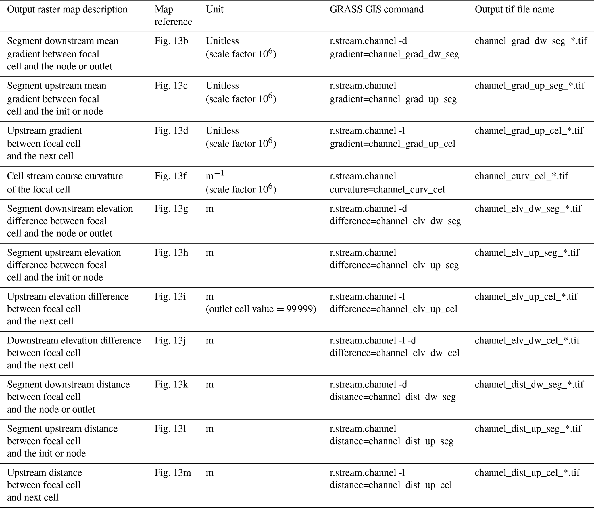
Table 6 Stream order raster and vector files computed with the r.stream.order GRASS GIS module, the map reference corresponding to Fig. 14, the specific GRASS GIS command, and the layer output name.

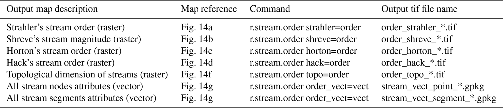
Figure 13 Map (a) shows the stream channels and drainage basins derived from the elevation layer. Maps (b)–(m) show, for the same area, the curvature, gradient (elevation difference divided by distance), and elevation change raster maps computed with r.stream.channel GRASS GIS module. The panel letters correspond to those in Table 5.

6.4 Stream order

We calculated a suite of topological stream order layers at the segment level. Stream order is depicted as a positive integer for indicating the level of branching in the river network (Zhang et al., 2007a; Scheidegger, 1965). There are various approaches to stream ordering, which either start from the source of the river or from the outlet. We used the r.stream.order (Jasiewicz and Metz, 2011) module and calculated stream order using the following methods: Strahler's (Strahler, 1957), Hortons's (Horton, 1945), Shereve's (Shreve, 1967), Hack's (Hack, 1957), and topological stream hierarchy (Marani et al., 1991). We provided each stream order layer as an individual raster file and all stream orders within the stream vector topology attribute table (Table 6). For all items reported in the stream vector topology attribute table, refer to the r.stream.order GRASS GIS manual page (https://grass.osgeo.org/grass78/manuals/addons/r.stream.order.html, last access: 5 October 2022). From a hydrography point of view, the stream order is used in the River Continuum Concept and therefore provides the basis for distinguishing ecological processes from headwaters to river mouths (Vannote et al., 1980; Thoms et al., 2018).

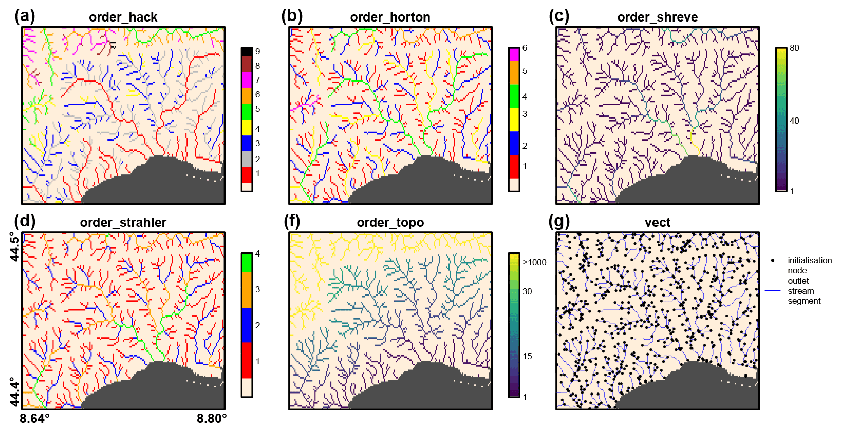
Figure 14 Maps (a)–(f) show different stream order types computed with the r.stream.order GRASS GIS module. All stream order layers are also available as vector data together with their attribute table. Map (g) shows the blue stream segments in vector format with the initialisation, node, and outlet vertices labelled as black points in Table 6.

6.5 Flow index

Using flow accumulation and terrain slope, we calculated three flow indices at the grid cell resolution: the compound topographic index (cti, or topographic wetness index), the stream power index (spi), and the stream transportation index (sti, Table 7).

The stream power index (spi) (Moore et al., 1991) is computed as the product of the upstream catchment area and the tangent of the terrain slope angle. The stream power index represents the erosive power associated with flow and the gravitational forces that move water downstream (Moore et al., 1991). It is commonly used in soil erosion models (Thalacker, 2014), landslide susceptibility (Pourghasemi et al., 2012), and groundwater estimations (Ozdemir, 2011).

The sediment transport index (sti) (Moore and Burch, 1986) is derived from unit stream power theory and is equivalent to the length–slope factor in the Revised Universal Soil Loss Equation (RUSLE) (Moore et al., 1991). It is often used to represent the erosive power of surface flow for landslides (Pourghasemi et al., 2012; Hong et al., 2017) or debris-flow modelling (Lay et al., 2019).

The compound topographic index (cti) (Beven and Kirkby, 1979), also known as topographic wetness index, is a steady state wetness index and is computed as the logarithm of the cumulative upstream catchment area divided by the tangent of the terrain slope angle. This index is a proxy for long-term soil moisture availability (Raduła et al., 2018). It has often been used in species distribution modelling, species richness and composition analyses, as well as landslide susceptibility and soil carbon assessments (Román-Sánchez et al., 2018; Raduła et al., 2018).

Table 7 The compound topographic index (cti), stream power index (spi), and stream transportation index (sti) derived from flow accumulation (α) and terrain slope (β); map reference corresponding to Fig. 15; unit; specific GDAL command; and output layer name.

7 Computational processing framework

In order to produce the standardised Hydrography90m products, we developed Bash scripts that launched each other in a cascading manner as a series of single batch jobs or as job arrays that submit and manage collections of similar jobs. The overall computation, starting from the calculation of flow accumulation to the topographic and topological variable creation (∼ 2TB of layer products), which accounted for a total of 52 scripts containing over 4 000 code lines, took 12 418 core hours at the High Performance Computing (HPC) facility of the Center for Research Computing, Yale University.

The entire procedure was run several times during computational development to check for consistency and potential mismatches among the different hydrographic layers. The scripts also employed several benchmarking strategies to check for potential errors in the data flow. The benchmarking strategies focused on:

• tile geographic extent at integer degree level;

• predefined ($\mathrm{0.0008}\stackrel{\mathrm{‾}}{\mathrm{3}}{}^{\circ }$) and constant cell resolution during the entire data processing;

• unique IDs for basins, sub-catchments, and stream segments worldwide;

• computation of histogram raster values to spot potential outliers;

• uniform tiling system for all layers;

• tile resampling at 30×30 arcsec ($\mathrm{0.008}\stackrel{\mathrm{‾}}{\mathrm{3}}{}^{\circ }$) cells for fast global visualisation;

• cross-over procedures to obtain consistent results (e.g. outlet number = drainage basins number; stream segments number = sub-catchments number).

8 Discussion

8.1 Methodological considerations

High-resolution information regarding the delineation of drainage basins and stream channels is vital for a wide array of earth system sciences, hydrology, chemistry, and freshwater biodiversity research as well as for informed management applications (Lowe and Likens, 2005; Reichl et al., 2009; Oudin et al., 2008; Maasri et al., 2021b; Amatulli et al., 2018b). Hydrography90m presents such information within a globally standardised and seamless hydrographic dataset that delineates headwaters in unparalleled detail. Hydrography90m is the first-ever data product that allows for global and comparative area-of-interest studies on small headwater stream channels. The high precision of the Hydrography90m has been demonstrated against NHDPlus HR and achieves high levels of accuracy for stream spatial and flow accumulation values. The increased density of headwaters in Hydrography90m, compared to the bench-mark NHDPlus HR and other reference hydrographies, is a distinctly valuable feature. These headwaters are a crucial component in hydrology and its associated applications (Lowe and Likens, 2005; Finn et al., 2011; Meyer et al., 2007) but have not been depicted globally until this publication. We thus opted for a comprehensive approach that enables headwater mapping at a high resolution. To achieve this objective, we delineated the potential headwater stream channels, which were derived entirely from DEM and topographic features.

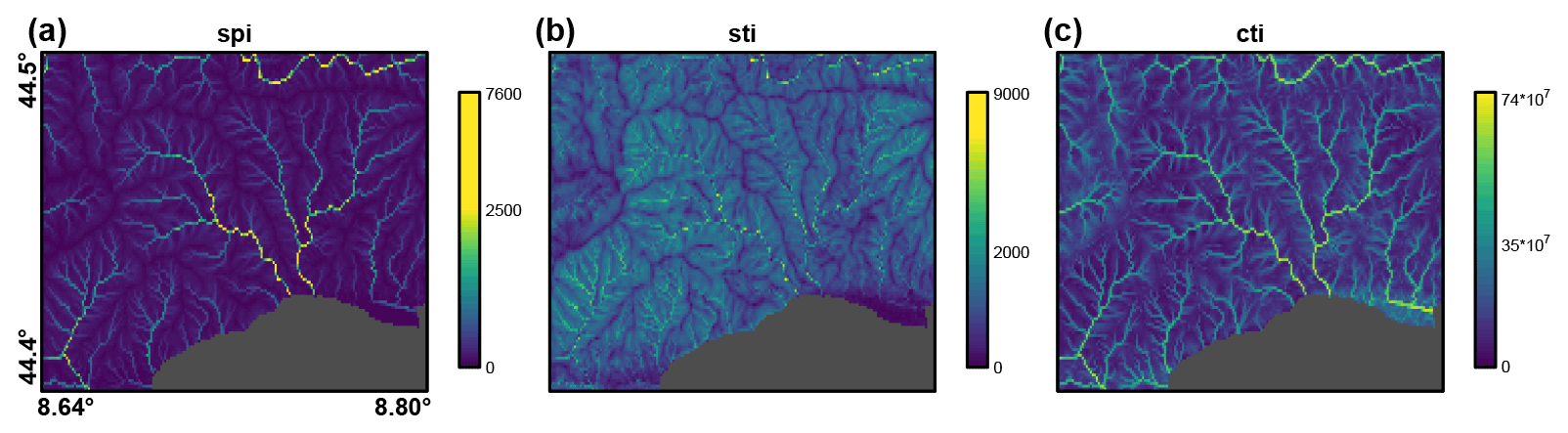
Figure 15 Different flow index layers computed using flow accumulation and terrain slope. Map (a) shows the stream power index (spi), map (b) sediment transport index (sti), and map (c) compound topographic index (cti). The panel letters correspond to those in Table  7.

Through the course of our ongoing research agenda, we will continue to identify unmapped perennial and non-perennial headwater channels by incorporating emerging higher-resolution DEMs (30 m) with benchmarking accuracy procedures (Strobl et al., 2021) and climatic and meteorological data. In arid regions, the delineated headwater stream channels receive water and produce floods (Farquharson et al., 1992), albeit with lower frequency compared to streams in humid and wet climates. However, these flow pulses are important for in-stream aquatic organisms (Bunn et al., 2006) and should not be neglected on a global stream network dataset. To address the frequency and duration of flows in these headwater streams, we are currently modelling discharge using a 30-year monthly climate time-series. This allows for the estimation of mean monthly discharge for each of the 726 723 221 identified stream segments and provides additional stream flow attributes to Hydrography90m. We shall thus be able to use this information to assign the probability of water occurrence to each stream channel, i.e. a stream channel will appear present if discharge >0 m³ s⁻¹. The overall outcome of this separate project will be a dynamic hydrological assessment, with stream channel length changing as a function of discharge. The final output will be monthly stream networks that are dynamic, i.e. longer during the rainy season and shorter and intermittent during dry months. Such monthly temporal assessment widens the scope for an improved and more complete representation of the network than assigning, for example, a channelisation threshold contingent on the geographic region alone, as suggested by Vogt et al. (2003). In summary, we employed a low threshold of 0.05 km² in this paper and, in subsequent research, will shorten (prune) the network dynamically, given the modelled discharge in the stream segments. Most importantly, the implementation of a low threshold allows the computation of topographic and topological variables for small headwater streams, which can be used to assess flow regimes and stream properties, such as sediment transportation. Pruning the network with a wider threshold in the first place would not allow the computation of such stream variables.

While Hydrography90m offers improved spatial accuracy compared to previous global hydrographic products, it can still benefit from several enhancements in the future. Currently, stream channel bifurcations are not represented in the Hydrography90m, and despite the MD8 algorithm distributing the flow accumulation to multiple grid cells, the stream channel follows only one downstream direction. We note that stream width was not considered in our approach, and due to the 3×3 arcsec spatial resolution, small headwater streams were located within grid cells. Standing water bodies were not yet integrated in Hydrography90m and are also part of our ongoing research. In the meantime, we invite users interested in integrating standing water bodies into Hydrography90m to contact the authors for a preliminary product.

Improvements to the state of the art are possible with even higher resolution digital terrain models than the employed MERIT Hydro. Nonetheless, increased resolution may also introduce the challenge of accounting for man-made canals and other engineered structures. For instance, we found in Hydrography90m that the Tongji Canal in China, part of the Grand Canal that connects the Yellow and Yangtze Rivers, routes sections of the Yellow's flow accumulation into the Yangtze, leading to discrepancies among the compared global hydrographic datasets (Table 2). Similarly, we identified missing bifurcations within the Niger river owing to the lack of bifurcation options in the implemented flow routing algorithm. While also a challenge in other global hydrographic datasets (Lehner et al., 2008; Yamazaki et al., 2019), missing bifurcation routines created difficulties with flow routing in Hydrography90m. Such bifurcations occurred mainly in very flat areas around the globe. Thus, any discharge computations derived from this dataset would need to account not only for missing bifurcations but also to apportion flow among two (or more) channels, according to each tributary's flow capacity.

8.2 Applications

Hydrography90m has been developed with a wide range of natural science applications in mind. In the broadest sense, its appeal lies in the potential for combining and extending the scope of both remote and field sensor technologies. The computational approach behind Hydrography90m not only overcomes spectral limitations but also the spatial and accessibility constraints of conventional resource monitoring instruments. While the dataset's uptake is obviously relevant within hydrography and hydrology, its value in numerous other geoinformatics applications is also well recognised.

The high-resolution base layers (flow accumulation and flow direction) and network hydrography layers (drainage basins, stream segments, and sub-catchments) can inform studies on flow estimation, sediment transport, and ecology. For example, flow accumulation has been utilised in flood susceptibility mapping models and often serves as a proxy for discharge in ecological modelling (Shafizadeh-Moghadam et al., 2018; Kuemmerlen et al., 2014). Flow direction has been used in metacommunity structure studies (Mozzaquattro et al., 2020), whereas drainage basins and sub-catchments can be used as the spatial units in species distribution modelling (Altermatt et al., 2013; Read et al., 2015). The Hydrography90m products can provide fundamental information for modelling the high-resolution supply and demand of biogeochemically relevant constituents that, so far, have been modelled using hydraulic information derived from low-resolution datasets (Raymond et al., 2016; Wollheim et al., 2018). These layers are a vital input in modelling species distribution (Domisch et al., 2019) and for monitoring invasive species (Haubrock et al., 2022), whether for biodiversity monitoring or for public health measures to combat vector-borne diseases (Bishop et al., 2021; Pless et al., 2021; Saarman et al., 2019, 2018). Specifically, sub-catchments have been used to derive zonal statistics from topographic and environmental layers for small-scale species distribution models (Kuemmerlen et al., 2014). Finally, this novel network has the appreciable potential to guide integrated freshwater conservation efforts, given its delineation of headwater stream channels, which are typically species rich (Abell et al., 2007).

Beyond their direct applications, the layers within Hydrography90m also offer important spatial and statistical information. For instance, the assessment of catchment similarity is useful for the prediction of ungauged basins (Reichl et al., 2009). Concurrently, in machine learning-based approaches, e.g. Long Short-Term Memory (LSTM) models (Kratzert et al., 2019), additional information on catchment attributes is highly sought after and advantageous to model accuracy.

Besides scientific studies, the aforementioned analyses would serve to address major geopolitical and natural resource challenges involving transboundary rights and water security, water resource management and food production (water quantity, quality, and nutrient flows), and catastrophe risk management (flooding, erosion, and drought), to name but a few. Nowadays, such issues notably fall under the ambit of several of the United Nations' Sustainable Development Goals (SDGs; Connor, 2015), such as the ones that concern water resource management, human health, peaceful and equitable societies, and sustainable economic development (Blöschl et al., 2017).

With regard to the methodology and computational process flows employed in Hydrography90m, we note below some key advantages as well as considerations for improvement. At the very outset of the dataset computation, a suite of topological and topographic feature layers accompany the base and network layers. While the former set of layers have been generated previously in coarse spatial resolutions (Lehner et al., 2008; Linke et al., 2019; Domisch et al., 2015a) or in higher regional to local resolutions (Domisch et al., 2015b), we anticipated that the more comprehensive, high-resolution layers of Hydrography90m will significantly reduce the burden of ad hoc, area-limited computations. Such globally available and analysis-ready data is also in line with our previously released http://spatial-ecology.net/docs/build/html/GEODATA/geomorpho90m/geomorpho90m.html (last access: 5 October 2022) (Amatulli et al., 2020) dataset, which seamlessly characterised global land surface using a collection of 26 http://hydro.iis.u-tokyo.ac.jp/~yamadai/MERIT_DEM/ (last access: 5 October 2022)-derived geomorphometry variables (Amatulli et al., 2020). The assimilation of this globally standardised data with various environmental, climate, stream flow (GSIM; Do et al., 2018; Gudmundsson et al., 2018), and freshwater quality observations (GRQA; Virro et al., 2021) provides the requisite quantum of inputs to implement a machine learning approach for high-resolution discharge and quality predictions.

9 Data availability

All metadata of the Hydrography90m dataset can be found at https://doi.org/10.18728/igb-fred-762.1 (Amatulli et al., 2022a). In the DOI's landing page are reported the links for the IGB-GeoNode visualisation and for the data storing repository. The repository includes a “README.txt file” that explains the folders' structure and file names. In addition, the data can be directly downloaded at http://hydrography.org (last access: 5 October 2022) by clicking on a given tile on the map.

The Hydrography90m dataset is protected by the Creative Commons Attribution-NonCommercial 4.0 International License (CC BY-NC 4.0), which permits sharing and adaption under the following terms: Attribution – you must give appropriate credit, provide a link to the license, and indicate if changes were made. You may do so in any reasonable manner, but not in any way that suggests the licensor endorses you or your use. Non-commercial – use of the material for commercial purposes is strictly prohibited, except with express permission from the licensor. To view a copy of this license, visit http://creativecommons.org/licenses/by-nc/4.0 (last access: 5 October 2022).

The article “Hydrography90m: a new high-resolution global hydrographic dataset” is licensed under the Creative Commons Attribution 4.0 International License. To view a copy of this license, visit http://creativecommons.org/licenses/by/4.0 (last access: 5 October 2022).

10 Code availability

At https://hydrography.org/hydrography90m/hydrography90m_workflow/ (Amatulli, 2022a) we report a schematic scripting procedure of the workflow together with an example to merge tiles and operate with regional units.

11 Conclusions

In this study, we constructed Hydrography90m as a globally seamless and standardised hydrographic network with associated stream topographic and topological features. These latter supplementary layers were carefully developed to ensure consistency and compatibility among all of the presented hydrography layers.

The data validation procedures confirmed Hydrography90m as a more accurate representation of stream networks compared to HydroRIVERS, GRWL, and MERIT Hydro–Vector. Improved accuracy was achieved principally by employing a higher resolution DEM, the MD8 flow routing algorithm, and a markedly smaller flow accumulation threshold to initiate stream channels. With these characteristics, Hydrography90m provides a valuable basis for supporting a variety of freshwater-related research disciplines.

Moreover, Hydrography90m is currently being further processed to (i) exclude the DEM-derived headwater streams that are not hydrologically relevant, (ii) include a suite of high-resolution (both spatial and temporal) environmental attributes for each of the 726 million stream segments, and (iii) integrate standing water bodies within the hydrographic network.

12 Usage notes

Below we report the web access points for data description and download.

• The Hydrography90m metadata are reported at https://doi.org/10.18728/igb-fred-762.1 (Amatulli et al., 2022a).

• The tiled Hydrography90m files are stored at https://public.igb-berlin.de/index.php/s/agciopgzXjWswF4 (last access: 5 October 2022) repository.

• The download procedure via a map interface is available at https://hydrography.org/hydrography90m/hydrography90m_layers/ (Hannon, 2022).

• The download procedure via a scripting routine is available at https://hydrography.org/hydrography90m/hydrography90m_layers/ (Amatulli, 2022b)

• The online visualisation of the layers via the IGB-GeoNode can be accessed via https://doi.org/10.18728/igb-fred-762.1 (Amatulli et al., 2022a).

The layers in Hydrography90m are compatible with any standard GIS application. We encourage, however, use of the open-source QGIS and GRASS GIS tools to further process the data. The benefit lies in the seamless integration with the processing algorithms as well as the identical spatial definition of the regional and grid cell extents.

Since we accounted for inland depressions, the stream channel network may terminate in these depression locations. We provide the regional unit layer (useful for extracting entire basins), allowing the seamless integration of those interior drainage basins into their surrounding and larger basin neighbourhoods.

For a given study area, we recommend users check the tile ID for the area of interest. The basins, stream channels, or sub-catchments will be split at the tile border, and a standard merge (raster) or dissolve by ID (vector) operation can mosaic the data together. If any smaller, surrounding drainage basins should be discarded, we then recommend masking the mosaicked tiles with the specific drainage basin IDs in the regional unit raster. This results in keeping only those drainage basins of interest. We provide example and helper functions for downloading, merging, cropping, and masking the data at http://hydrography.org (last access: 5 October 2022).