A 10-year global monthly averaged terrestrial net ecosystem exchange dataset inferred from the ACOS GOSAT v9 XCO₂ retrievals (GCAS2021)

A global gridded net ecosystem exchange (NEE) of CO₂ dataset is vital in global and regional carbon cycle studies. Top-down atmospheric inversion is one of the major methods to estimate the global NEE; however, the existing global NEE datasets generated through inversion from conventional CO₂ observations have large uncertainties in places where observational data are sparse. Here, by assimilating the GOSAT ACOS v9 XCO₂ product, we generate a 10-year (2010–2019) global monthly terrestrial NEE dataset using the Global Carbon Assimilation System, version 2 (GCASv2), which is named GCAS2021. It includes gridded ($\mathrm{1}{}^{\circ }\times \mathrm{1}{}^{\circ }$), globally, latitudinally, and regionally aggregated prior and posterior NEE and ocean (OCN) fluxes and prescribed wildfire (FIRE) and fossil fuel and cement (FFC) carbon emissions. Globally, the decadal mean NEE is $-\mathrm{3.73}\pm \mathrm{0.52}$ PgC yr⁻¹, with an interannual amplitude of 2.73 PgC yr⁻¹. Combining the OCN flux and FIRE and FFC emissions, the net biosphere flux (NBE) and atmospheric growth rate (AGR) as well as their inter-annual variabilities (IAVs) agree well with the estimates of the Global Carbon Budget 2020. Regionally, our dataset shows that eastern North America, the Amazon, the Congo Basin, Europe, boreal forests, southern China, and Southeast Asia are carbon sinks, while the western United States, African grasslands, Brazilian plateaus, and parts of South Asia are carbon sources. In the TRANSCOM land regions, the NBEs of temperate N. America, northern Africa, and boreal Asia are between the estimates of CMS-Flux NBE 2020 and CT2019B, and those in temperate Asia, Europe, and Southeast Asia are consistent with CMS-Flux NBE 2020 but significantly different from CT2019B. In the RECCAP2 regions, except for Africa and South Asia, the NBEs are comparable with the latest bottom-up estimate of Ciais et al. (2021). Compared with previous studies, the IAVs and seasonal cycles of NEE of this dataset could clearly reflect the impacts of extreme climates and large-scale climate anomalies on the carbon flux. The evaluations also show that the posterior CO₂ concentrations at remote sites and on a regional scale, as well as on vertical CO₂ profiles in the Asia-Pacific region, are all consistent with independent CO₂ measurements from surface flask and aircraft CO₂ observations, indicating that this dataset captures surface carbon fluxes well. We believe that this dataset can contribute to regional- or national-scale carbon cycle and carbon neutrality assessment and carbon dynamics research. The dataset can be accessed at https://doi.org/10.5281/zenodo.5829774 (Jiang, 2022).

1 Introduction

The terrestrial ecosystem uptakes CO₂ from the atmosphere through photosynthesis and releases CO₂ into the atmosphere through respiration. Its net ecosystem exchange (NEE) plays a very important role in regulating the atmospheric CO₂ concentration, thereby slowing down global warming. However, NEE has significant spatial differences and inter-annual variations (IAVs) (Bousquet et al., 2000; Piao et al., 2020). Therefore, accurately quantifying global and regional NEE and clarifying the drivers of IAV are key scientific issues in global carbon cycle research, and a reliable global NEE dataset is vital for this research.

Until now, a series of global NEE or net biosphere exchange (NBE = NEE + wildfire carbon emission) products like FLUXCOM (Jung et al., 2009), TRENDY (Sitch et al., 2015), Jena CarboScope (Rödenbeck et al., 2003), CT2019B (Jacobson et al., 2020), and CMS-Flux NBE 2020 (Liu et al., 2021), have been available and widely used in different studies, which were created using data-driven machine learning methods, ecosystem models, or inversion models. Machine learning methods estimate the global carbon flux by upscaling eddy covariance data (Zeng et al., 2020); ecosystem models simulate photosynthesis and respiration of ecosystems based on meteorological, soil, and land cover data and a series of parameters (Chen et al., 1999); and inversion models estimate surface CO₂ fluxes using the globally distributed atmospheric CO₂ observations and/or satellite retrievals of column-averaged CO₂ dry air mole fraction (XCO₂) (Enting and Newsam, 1990; Gurney et al., 2002; Jiang et al., 2021). Different methods have their own advantages and disadvantages. The NEE estimated by top-down atmospheric inversions is determined by the density and accuracy of the CO₂ observations, the accuracy of modeled atmospheric transport, and knowledge of the prior uncertainties of the flux inventories (Liu et al., 2021). Generally, in situ and flask CO₂ observations have high precision, with measurement error lower than 0.2 ppm; however, the global distribution of flask or in situ sites is extremely uneven. There are many sites over North America (N. America) and Europe but very few sites over the tropics, Africa, and southern oceans (Schuldt et al., 2020). Therefore, the inversions generally have a robust performance on a global or hemisphere scale (Houweling et al., 2015), but on regional scales, due to the uneven distribution of observations, the reliability of inversion results varies greatly in different regions (Peylin el al., 2013).

Satellite XCO₂ retrievals from the Greenhouse Gases Observing Satellite (GOSAT) (Kuze et al., 2009) and the Observing Carbon Observatory 2 (OCO-2) (Crisp et al., 2017) have much better spatial coverage (O'Dell et al., 2018) than ground-based observations. Although the accuracy of XCO₂ is relatively lower (∼1 ppm, Kulawik et al., 2019) compared to flask and in situ observations, and the response of XCO₂ to changes in the surface carbon flux is weaker, many inversion studies have proved that satellite XCO₂ retrievals could improve the estimates of surface carbon fluxes (e.g., Basu et al., 2013; Maksyutov et al., 2013; Saeki et al., 2013; Chevallier et al., 2014; Deng et al., 2016), especially for the fluxes in Africa, South America (S. America), and Asia, where the sparsity of the surface monitoring sites is most evident (Takagi et al., 2011). Wang et al. (2019) compared the NEE inferred from GOSAT and OCO-2 retrievals and surface flask observations and found that the performance of inversion with GOSAT data only was comparable with the one using surface observations. Moreover, studies also showed that with satellite XCO₂ retrievals, the inverted carbon flux could well reveal the impact of extreme droughts and large-scale climate anomalies on regional and continental terrestrial carbon dynamics (Liu et al., 2018; Deng et al., 2016; Detmers et al., 2015; Jiang et al., 2021).

By assimilating both GOSAT and OCO-2 XCO₂ retrievals, Liu et al. (2021) generated a global gridded monthly NBE product (i.e., CMS-Flux NBE 2020) using the NASA Carbon Monitoring System Flux (CMS-Flux) inversion framework (Liu et al., 2014, 2017, 2018; Bowman et al., 2017). This dataset spans 2010–2018, in which the data from 2010–2014 and 2015–2018 were inferred from GOSAT XCO₂ and OCO-2 data, respectively. GOSAT and OCO-2 XCO₂ have large differences on spatial resolution and coverage, which may lead to discontinuities in the inversion results of certain regions. The ACOS GOSAT v9 XCO₂ data are now available on the NASA Goddard Earth Science Data and Information Services Center (GES-DISC), which spans April 2009 to June 2020 and has been bias-corrected and quality-filtered well (Taylor et al., 2022). In this study, based on the GOSAT v9 XCO₂ retrievals, we generate a 10-year global monthly NEE dataset from 2010 to 2019 (GCAS2021) using the well-constructed Global Carbon Assimilation System, version 2 (GCASv2) (Jiang et al., 2021; Wang et al., 2021a). Different from Liu et al. (2021), GCAS2021 focuses on NEE because the wildfire (FIRE) emission was not optimized in this study. The optimized ocean flux and prescribed FIRE and fossil fuel and cement carbon (FFC) emissions are also included in this dataset. Users who want to use NBE data could combine the NEE and FIRE emission by themselves. It is worth pointing out that since we have not optimized FIRE emissions, the optimized NEE may include compensation for the errors in FIRE emissions. This paper is organized as follows: Sect. 2 details the GOSAT retrievals, prior fluxes, and the GCASv2 system as well as uncertainty settings. Section 3 introduces the evaluation data and method, Sect. 4 briefly describes the dataset, Sect. 5 presents the characteristics of the dataset, including the estimates of global carbon budget and regional NEE as well as their IAVs, Sect. 6 details the evaluations results against independent CO₂ observations, and Sect. 7 gives a summary and the main conclusions.

2 Methods and data

2.1 The ACOS v9 GOSAT XCO₂ retrievals

The GOSAT satellite launched in 2009 (Kuze et al., 2009) was developed jointly by the National Institute for Environmental Studies (NIES), the Japanese Space Agency (JAXA), and the Ministry of the Environment (MOE) of Japan, which was designed to retrieve total column abundances of CO₂ and CH₄. In this study, the GOSAT XCO₂ retrieval is the ACOS Version 9.0 Level 2 Lite product (Taylor et al., 2022) at the pixel level during May 2009–December 2019. The bias correction and quality filtering of this XCO₂ product have been evaluated using estimates derived from the Total Carbon Column Observing Network (TCCON) as well as values simulated from a suite of global atmospheric inverse modeling systems (models); the results show that the differences in XCO₂ between GOSAT v9 and both TCCON and models have an 1σ error of approximately 1 ppm for ocean-glint observations and 1 to 1.5 ppm for land observations, and globally, the mean biases are less than approximately 0.2 ppm (Taylor et al., 2022). Compared with its previous version (ACOS v7.3), the proportion of data with a “good” XCO₂ quality flag has increased from 3.9 % in v7.3 to 5.4 % in v9.

The GOSAT XCO₂ retrievals have a resolution of 10.5 km² at nadir. Considering the fact that the resolution of a global atmospheric transport model is significantly lower than that of XCO₂ retrievals, we re-grid the XCO₂ data into $\mathrm{1}{}^{\circ }\times \mathrm{1}{}^{\circ }$ grid cells. The pixel level XCO₂ data are filtered with the xco2_quality_flag, which is a simple quality flag denoting science quality data (0= good, 1= bad), provided along with the XCO₂ product. In each $\mathrm{1}{}^{\circ }\times \mathrm{1}{}^{\circ }$ grid and each day, only the XCO₂ with an xco2_quality_flag equal to 0 is selected and averaged according to Eq. (1).

$$\begin{array}{}\text{(1)}& C_{G,T}={\displaystyle \frac{\mathrm{1}}{W}}{\sum }_{l=\mathrm{1}}^W{C}_{l,t},T={\displaystyle \frac{\mathrm{1}}{W}}{\sum }_{l=\mathrm{1}}^{W}t,\end{array}$$

where C_l,t denotes the selected pixel level XCO₂ located in $\mathrm{1}{}^{\circ }\times \mathrm{1}{}^{\circ }$ grid G of 1 d, l is the identifier of the record, t is the observation time, and W denotes the number of C_l,t. T is the averaged observation time, and C_G,T is the re-grided XCO₂ concentrations. The other variables in the XCO₂ product like column-averaging kernel and retrieval error, which will be used in the calculations of simulated XCO₂, are also re-gridded using this method.

2.2 Prior CO₂ fluxes

The prior carbon fluxes used in this study consist of terrestrial NEE, FIRE carbon emission, FFC carbon emission, and CO₂ exchanges over the ocean surface (OCN). NEE in a 3 h interval is simulated using the Boreal Ecosystems Productivity Simulator (BEPS) model; for details about the BEPS simulations, please refer to Chen et al. (2019). FIRE emission is directly obtained from the Global Fire Emissions Database, Version 4.1 (GFED4s) (van der Werf et al., 2017; Mu et al., 2011). FFC emission is an average of two products from Carbon Dioxide Information Analysis Center (CDIAC) (Andres et al., 2011) and Open-source Data Inventory of Anthropogenic CO₂ (ODIAC) (Oda et al., 2018), respectively. OCN flux is derived from the Takahashi et al. (2009) climatology of seawater pCO₂. Both FFC emission and OCN flux were downloaded from CT2019B (Jacobson et al., 2020). It should be noted that there are no data in the pCO₂-Clim product in many offshore areas like the Sea of Japan, the Mediterranean, the Gulf of Mexico, and the East China Sea. Following Jiang et al. (2021), the fluxes in 2009 modeled using a combined global ocean circulation (OPA) and biogeochemistry model (PISCES-T) (Buitenhuis et al., 2006) are used to fill the no-data areas. The sea–air CO₂ fluxes simulated using the PISCES-T model have been used in many studies of ocean carbon cycle dynamics (e.g., McKinley et al., 2006; Valsala et al., 2012; Le Quéré et al., 2007) and also used as a priori ocean fluxes in previous inversion studies (e.g., Jiang et al., 2014; Deng and Chen, 2011; Chen et al., 2017). In addition, the CT2019B product is only until the beginning of 2019. The OCN flux in 2019 is assumed to be the same as 2018. FFC emission is adjusted from the emission in 2018 by ratios of 2019/2018 in different countries or regions (Fig. S1 in the Supplement), which was calculated based on the 2018 and 2019 emissions compiled by the Global Carbon Budget 2020 (GCP2020; Friedlingstein et al., 2020).

2.3 The Global Carbon Assimilation System (GCAS), version 2

The global monthly NEE dataset is inferred using the Global Carbon Assimilation System, version 2 (GCASv2), which was developed for estimating gridded surface carbon fluxes, mainly using satellite XCO₂ retrievals (Jiang et al., 2021). In this system, the Model for Ozone and Related Chemical Tracers, version 4 (MOZART-4) (Emmons et al., 2010), was coupled to simulate 3-D atmospheric CO₂ concentrations, and the ensemble square root filter (EnSRF) algorithm (Whitaker and Hamill, 2002) was used to implement the inversion of surface fluxes. GCASv2 runs cyclically, and in each cycle (DA window), we use a “two-step” calculation scheme to maintain quality conservation. First, the prior fluxes are optimized using XCO₂ data, and then, the optimized fluxes are put again into the MOZART-4 model to generate the initial condition (IC) of the next window. In order to reduce the representative error of XCO₂, a “super-observation” approach is also adopted, in which a super-observation is generated by averaging all observations located within the same model grid within a DA window; and to reduce the impact of spurious correlations, a localization technique is employed to determine which super-observations will be used for the current grid's optimization, which is based on the correlation coefficient between the simulated concentration ensembles in each observation location and the perturbed fluxes in current model grids and their distances. For details, please refer to Jiang et al. (2021).

In this study, GCASv2 was run from 1 May 2009 to 31 December 2019 with the DA window of 1 week. The IC of 3-D CO₂ concentrations at 00:00 UTC 1 May 2009 was obtained from the product of CarbonTracker, version 2017 (CT2017). The first 8 months are considered as a spin-up run, and the results from 1 January 2010 to 31 December 2019 are analyzed and evaluated in this study. MOZART-4 is driven by the GEOS-5 meteorological fields, which have a spatial resolution of $\mathrm{1.9}{}^{\circ }\times \mathrm{2.5}{}^{\circ }$ and a vertical level of 72 layers (Tilmes, 2016). MOZART-4 uses the same spatial resolution and the lowest 56 vertical levels of GEOS-5. Following Jiang et al. (2021), the model–data mismatch error of XCO₂ is constructed using the XCO₂ retrieval errors, which are provided along with the XCO₂ product and re-gridded using the same method as described in Sect. 2.1. All retrieval errors are also uniformly inflated by a factor of 1.9 in this study, but a lowest error is fixed as 1 ppm.

There are four state vectors combining schemes in GCASv2, including the following: (1) only the NEE is treated as a state vector and optimized; (2) both NEE and OCN flux are state vectors; (3) NEE, OCN flux, and FFC emissions are optimized at the same time; and (4) only the net flux is optimized. In this study, the second scheme was selected: both NEE and ocean flux are optimized, and the FIRE and FFC are prescribed. The perturbation of prior fluxes is described in Eq. (2), where δ_i represents random perturbation samples and is drawn from Gaussian distributions with mean zero and standard deviation of 1. i is the identifier of the perturbed samples, N is the ensemble size (here 50). λ is a set of scaling factors, which represents the uncertainty of each prior flux. $X_{\mathrm{NEE}}^b$, $X_{\mathrm{FIRE}}^b$, $X_{\mathrm{FFC}}^b$, and $X_{\mathrm{OCN}}^b$ represent the prior fluxes of NEE, FIRE, FFC, and OCN, respectively. The spatial resolution of the perturbation factor (δ_i×λ) we adopted is $\mathrm{3}{}^{\circ }\times \mathrm{3}{}^{\circ }$, and the resolution of the prior fluxes is $\mathrm{1}{}^{\circ }\times \mathrm{1}{}^{\circ }$; that is, the prior fluxes within each 3^∘ grid have the same perturbation factor. In each 3^∘ grid, λ_NEE and λ_ocn are set to be 6 and 10, respectively, which correspond to a global 1−δ uncertainty of the NEE and OCN flux of about 0.6 and 0.2 PgC yr⁻¹, respectively (for the method, see Sect. S1 in the Supplement).

$$\begin{array}{}\text{(2)}& \begin{array}{rl}{\mathbf{X}}_i^b& ={\mathit{\lambda }}_{\mathrm{NEE}}\times {\mathit{\delta }}_{i,\mathrm{NEE}}\times {\mathbf{X}}_{\mathrm{NEE}}^b+{\mathit{\lambda }}_{\mathrm{ocn}}\times {\mathit{\delta }}_{i,\mathrm{ocn}}\times {\mathbf{X}}_{\mathrm{OCN}}^b\\ & +{\mathbf{X}}_{\mathrm{Fire}}^b+{\mathbf{X}}_{\mathrm{FFC}}^b,i=\mathrm{1},\mathrm{2},\mathrm{\dots },N\end{array}\end{array}$$

3 Evaluation data and method

Due to the huge difference of spatial scale between the inverted and directly observed fluxes, generally, it is impossible to directly validate the posterior NEE using observations, and instead, we indirectly evaluate the posterior flux by comparing the forward simulated atmospheric CO₂ mixing ratios against independent CO₂ measurements (e.g., Jiang et al., 2021; Wang et al., 2019; Feng et al., 2020). Therefore, a forward simulation using the MOZART-4 model and the posterior fluxes was conducted to create posterior CO₂ concentrations. For comparison, the prior CO₂ concentrations were also simulated with the prior fluxes. The simulation period and model configuration of MOZART-4 as well as initial field are the same as the assimilation experiment as described in Sect. 2.3.

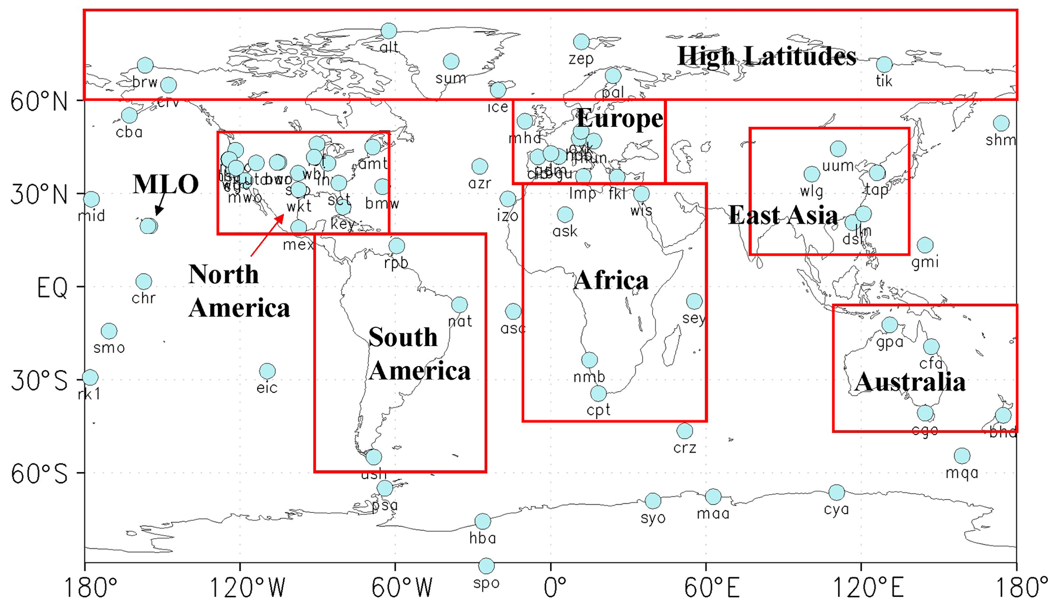
Figure 1 Distributions of the surface flask observation sites used in this study.

Surface flask and aircraft CO₂ observations are used for these independent evaluations in this study, which were obtained from the obspack_co2_1_GLOBALVIEWplus_v6.0_2020-09-11 product (OBSPACKv6; Schuldt et al., 2020). OBSPACKv6 contains a collection of discrete (flask), programmable flask package (PFP), and quasi-continuous (in situ) measurements at surface, tower, ship, and aircraft sites contributed by national and universities laboratories around the world. In this study, surface flask CO₂ measurements (including surface PFP) from 74 sites and aircraft measurements (including flask, PFP, and in situ measurement methods) from three projects are selected to evaluate the posterior CO₂ concentrations. There are 148 surface flask and PFP sites of observations in OBSPACKv6. The 74 sites were selected according to the following processes: (1) only the sites with data more than 7 years during 2010–2019 were selected (48 sites removed); (2) for one location, if there are observations from different institutes, only the data provided by the NOAA Global Monitoring Laboratory (with lab number of 1 in each filename) were selected (21 sites removed); (3) for one location, if both flask and PFP observations are available, only flask observations were adopted (1 site removed); (4) for the PFP site, if there are observations at different heights, only the observations at the top level were used (1 site removed); and (5) during the evaluations, we find that MOZART-4 model is unable to capture the variations of CO₂ mixing ratios at BKT and LJO; thus these sites were also removed. The locations of the 74 sites are shown in Fig. 1, and the corresponding site codes as well as information about latitude and longitude are listed in Table S1 in the Supplement.

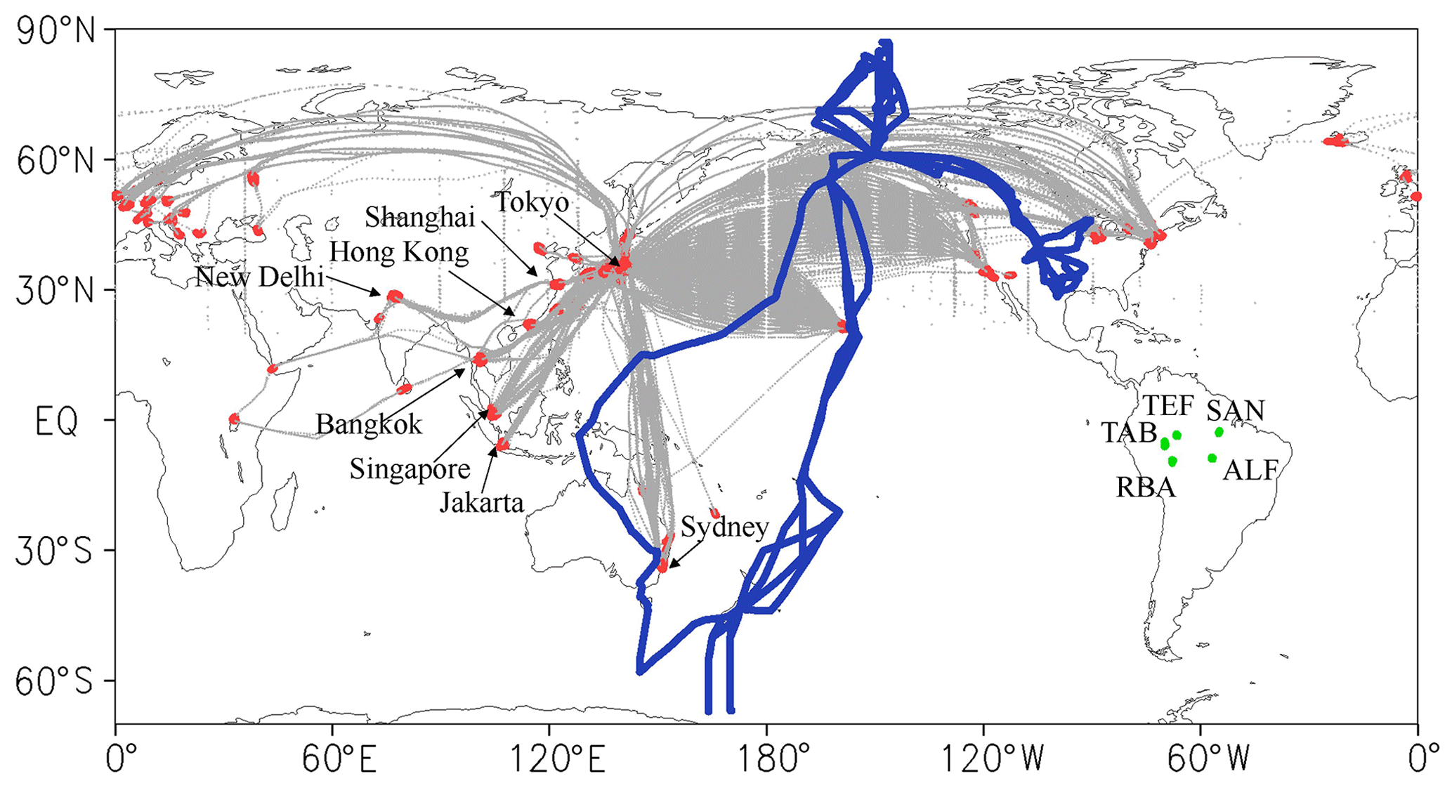
Figure 2 Locations of aircraft observations (red and gray, observations of the CONTRAIL project; red marks show observations below 6 km, dark blue observations of the HIPPO project, and green data of the CARBAM project).

There are 76 aircraft observation sites (independent data files) in OBSPACKv6. In this study, we chose observations from the Comprehensive Observation Network for Trace gases by Airliner (CONTRAIL) project (Machida et al., 2008, 2018; Matsueda et al., 2008, 2015), the HIAPER Pole-to-Pole Observations (HIPPO) program (Wofsy, 2011), and the lower-troposphere greenhouse-gas sampling program in the Amazon basin of the CARBAM project (Gatti et al., 2014, 2021) to further evaluate the posterior CO₂ concentrations. The CONTRAIL project measures CO₂ concentrations using Continuous CO₂ Measuring Equipment (CME) on two passenger aircraft (Boeing 747-400 and 777-200ER); thus there are observations along flight paths (including level flight, taking off, and landing) from Japan to N. America, to Europe, to Hawaii, to Australia, and to Southeast and South Asia (Fig. 2). During the taking off and landing, vertical profiles of CO₂ concentrations near airports were observed. As shown in Fig. 1, there are few surface observations over the Asia-Pacific region, especially in Southeast and South Asia; therefore, the CO₂ vertical profiles near eight cities over the Asia-Pacific region are selected in this study. The eight cities are Hong Kong, Singapore, Jakarta, Bangkok, Sydney, New Delhi, Shanghai, and Tokyo. The HIPPO program completed aircraft measurements spanning the Pacific from 85^∘ N to 67^∘ S during the periods of March to April 2010 and June to September 2011, with vertical profiles every approximately 2.2^∘ of latitude (Wofsy, 2011). The CARBAM project conducted vertical CO₂ measurements at four sites (i.e., ALF, RBA, SAN, TAB, and TEF) in the Amazon basin during 2010–2018 (Fig. 2) with small aircraft and PFP equipment. TAB was from 2010 to 2012, and TEF started in 2013. During the evaluation of this study, TAB and TEF are combined as one site, denoted TAB_TEF. At each site, one to three spiral profiles from approximately 4420 to about 300 m a.s.l. were observed in each month. It is worth noting that OBSPACKv6 only provides ALF, RBA, SAN, and TAB observations from 2010 to 2012; the rest of the data were downloaded from Gatti et al. (2021). For the CONTRAIL vertical profiles, the observations between the heights of 2 and 6 km are used because the data measured below 2000 m are highly affected by local emissions (Jiang et al., 2014) due to the frequently ascent and descent of aircraft. And for the HIPPO and CARBAM observations, the data above 1 km are adopted.

Four basic statistical measures, i.e., mean bias (BIAS), mean absolute error (MAE), root mean square error (RMSE), and correlation coefficient (CORR), are calculated against the surface and aircraft CO₂ observations, respectively. The functions of these four basic statistical measures are expressed as

$$\begin{array}{}\text{(3)}& {\displaystyle }\mathrm{BIAS}={\displaystyle \frac{\mathrm{1}}{M}}{\sum }_{j=\mathrm{1}}^M\left(x_j-y_j\right)=\overline{y}-\overline{x}\text{(4)}& {\displaystyle }\mathrm{MAE}={\displaystyle \frac{\mathrm{1}}{M}}{\sum }_{j=\mathrm{1}}^M|x_j-y_j|\text{(5)}& {\displaystyle }\mathrm{RMSE}=\sqrt{{\displaystyle \frac{\mathrm{1}}{M}}{\sum }_{j=\mathrm{1}}^M{\left(x_j-y_j\right)}^{\mathrm{2}}}\text{(6)}& {\displaystyle }\mathrm{CORR}={\displaystyle \frac{{\sum }_{j=\mathrm{1}}^M(x_j-\overline{x})(y_j-\overline{y})}{\sqrt{{\sum }_{j=\mathrm{1}}^M(x_j-\overline{x}{)}^{\mathrm{2}}}\sqrt{{\sum }_{j=\mathrm{1}}^M(y_j-\overline{y}{)}^{\mathrm{2}}}}},\end{array}$$

where x_j and y_j denote the modeled and the observational values, respectively, at the jth out of M records, and the overbars denote averages. The BIAS, MAE, RMSE, and CORR reflect the overall model tendency, both the model bias and error variance, and the linear correspondence between the modeled and observational values, respectively.

4 Dataset description

GCAS2021 includes (1) monthly and annual prior and posterior NEE and OCN fluxes and prescribed FIRE and FFC emissions in a global spatial resolution of $\mathrm{1}{}^{\circ }\times \mathrm{1}{}^{\circ }$; (2) globally, latitudinally, and regionally aggregated monthly and annual posterior NEE and NBE and their uncertainties; and (3) weekly gridded ensemble members of posterior NEE and OCN fluxes. The regional fluxes are aggregated both in the TRANSCOM (Gurney et al., 2003) and the REgional Carbon Cycle Assessment and Processes Project (RECCAP2; Ciais et al., 2022) regions (Fig. 3). The latitudinal fluxes are aggregated in northern midlatitudes to high latitudes (>30^∘ N, NL), tropical latitudes (30^∘ S–30^∘ N, TL), and southern middle latitudes ($<\mathrm{30}{}^{\circ }$ N, SL). The weekly gridded ensemble members could be used for calculating the posterior uncertainties based on user defined regional masks. We also provide a Fortran program for the calculation of posterior uncertainties. The method for calculating posterior uncertainties is given in Sect. S1. The gridded data are in NetCDF-3 format, while the regional aggregated data are in .xlsx format.

Table 1 Global carbon budget (PgC yr⁻¹).

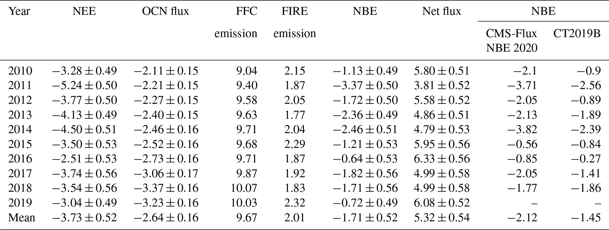
Figure 3 Map of regional masks used in calculating regional fluxes: (a) the TRANSCOM region and (b) the RECCAP2 region.

5 Characteristics of the dataset

5.1 Global carbon budgets

Table 1 presents the year-by-year and decadal averaged posterior global carbon budgets during 2010–2019 of this study. The global annual NEE is in the range of $-\mathrm{2.51}\pm \mathrm{0.53}$ to $-\mathrm{5.24}\pm \mathrm{0.50}$ PgC yr⁻¹ (negative means absorbing CO₂ from the atmosphere, and positive means releasing CO₂ to the atmosphere). The year of 2011 has the largest land sink in the decade, while the year of 2016 has the weakest one, with interannual amplitude reaching 2.73 PgC yr⁻¹. On average, the decadal mean NEE is $-\mathrm{3.73}\pm \mathrm{0.52}$ PgC yr⁻¹. The OCN flux has an overall increase trend from 2010 to 2009, with a mean of $-\mathrm{2.64}\pm \mathrm{0.16}$ PgC yr⁻¹. Compared with the prior NEE (Fig. S9l), the posterior NEEs increase significantly from 2010 to 2012 and decrease to varying degrees (in range of 0.15 to 1.15 PgC yr⁻¹) from 2015 to 2019. Table 1 also lists the estimates from the CMS-Flux (CMS-Flux NBE 2020, Liu et al., 2021) and CarbonTracker (CT2019B, Jacobson et al., 2020) systems. CMS-Flux NBE 2020 is a product for the period of 2010–2018, in which the results of 2010–2014 were inverted from the GOSAT XCO₂ v7.3, and the rest were inferred from the OCO-2 XCO₂ v9 retrievals. Both GOSAT and OCO-2 retrievals were from the ACOS team, created using the same retrieval algorithm and validated using the same strategy (Liu et al., 2021). CT2019B is a product inverted from global surface, tower, and aircraft CO₂ measurements. CMS-Flux NBE 2020 only presented the NBE results, and the FIRE emission used in this study and CT2019B are also different. Therefore, this comparison focuses on NBE. In 2010 and 2014, our estimates are close to CT2019B and significantly lower than the estimates of CMS-Flux NBE 2020; in contrast, in 2011, 2012, 2013, 2016, and 2017, they are comparable to CMS-Flux NBE 2020 and higher than those of CT2019B. In 2015, it is higher than both. Moreover, Fig. 4 presents a comparison between the estimates of this study and GCP2020 (Friedlingstein et al., 2020). There are large differences for the land-use and land-cover change (LULCC) carbon emissions between this study and GCP2020; we directly use the FIRE emission from GFED 4.1s as prescribed land-use emission, while GCP2020 uses an average of three bookkeeping models (Houghton and Nassikas, 2017; Hansis et al., 2015; Gasser et al., 2020), which account for changes in all carbon pools affected by LULCC. Therefore, we also compared the NBE between this study and GCP2020. For GCP2020, the NBE is the sum of NEE and LULCC emissions. Additionally, GCP2020 also reported the atmospheric growth rate (AGR) of CO₂ in the atmosphere, which was estimated directly from atmospheric CO₂ concentration measurements provided by the NOAA Earth System Research Laboratory (Friedlingstein et al., 2020). Ideally, the inverted global net carbon flux (i.e., AGR) should agree with the observed AGR. As shown in Fig. 4, the interannual changes of global NBE and AGR of this study match well with the estimates of GCP2020, with CORR of 0.75 and 0.88, BIAS (this study minus GCP2020) of 0.15 and 0.25 PgC yr⁻¹, and MAE of 0.51 and 0.40 PgC yr⁻¹, respectively. The difference in NBE between this study and GCP2020 is partly due to the imbalance item in GCP2020, especially in 2016. It also should be noted that in this study, the AGR in 2019 is higher than that in 2015 and significantly higher than the observed value, which is mainly due to the abnormally low carbon sink in the tropical latitudes (TL, 30^∘ S–30^∘ N) in this year (Fig. 7). The reason may be related to the biases in the GOSAT XCO₂ retrievals in TL. We analyze the monthly changes of GOSAT XCO₂ in 2015 and 2019 and compare them with the OCO-2 XCO₂ retrievals (OCO-2 v10, OCO-2 Science Team, 2020). We find that after detrending, in TL, the GOSAT XCO₂ in 2019 is higher than that in 2015, while OCO-2 is the opposite (Fig. S3). For the prior fluxes, the CORR, BIAS, and MAE of NBE and AGR compared against the GCP2020 estimates are 0.16 and 0.49, −0.51 and 0.09 PgC yr⁻¹, and 0.63 and 1.10 PgC yr⁻¹ (Fig. S2). These indicate that the estimate of global carbon budgets has been significantly improved after being constrained by the GOSAT retrievals.

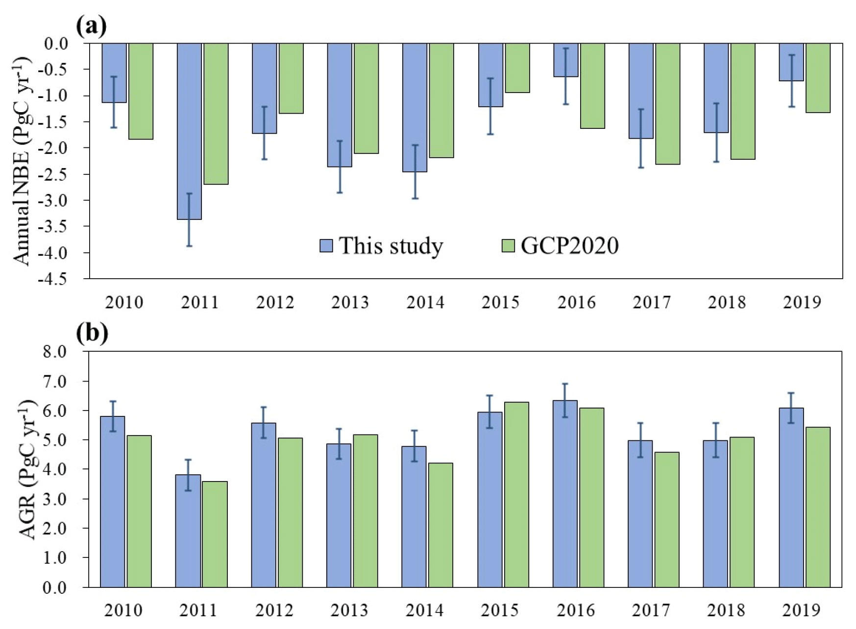
Figure 4 Comparisons between this study and GCP2020 for (a) NBE and (b) atmospheric growth rate (AGR); the NBE of GCP2020 is the sum of land sink and land-use change carbon emission, and the AGR of this study is the net flux as listed in Table 1.

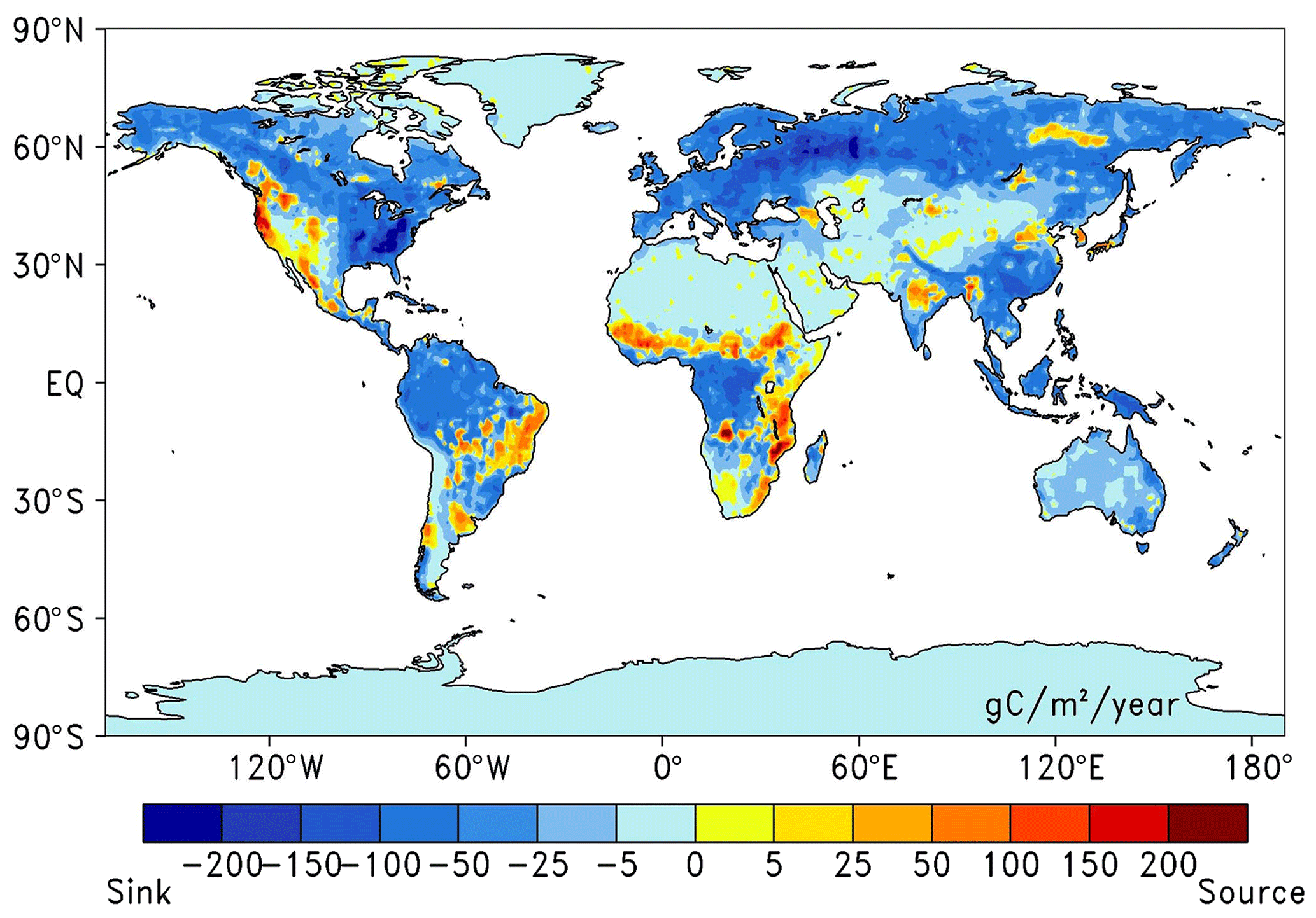
Figure 5 Global distribution of mean annual NEE during 2010–2019.

5.2 Annual NEE averaged from 2010–2019

Figure 5 shows the distributions of the mean posterior annual NEE during 2010–2019. Carbon uptakes mainly occur over eastern N. America, the Amazon, the Congo Basin, Europe, boreal forests, southern China, and Southeast Asia; and carbon releases mainly occur in western N. America (mainly the western United States), the East African and Ethiopian plateaus and the Sahel region (mainly the grasslands in Africa), the Brazilian plateau, and parts of South Asia. Compared with the prior NEE, the land sinks in western N. America, most of S. America, the grasslands in Africa, most of East and South Asia, and eastern Siberia are decreased, while the sinks in eastern N. America, Europe, and western Siberia are significantly increased (Fig. S4). In N. America, the distribution of NEE constrained with GOSAT XCO₂ exhibits a similar pattern to that of a recent regional inversion using surface CO₂ and ¹⁴CO₂ measurements, which also showed significant sources over the western United States and sinks over central and eastern United States (Basu et al., 2020). Using the Community Land Model (CLM5.0) and a Data Assimilation Research Testbed (DART) that were assimilated with remotely sensed observations of leaf area and above-ground biomass, Raczka et al. (2021) simulated the NEE over the western United States and also found that there are large areas with carbon release. The western United States is dominated by natural lands, which are particularly vulnerable to forest mortality from droughts, insect attacks, and wildfires. Ghimire et al. (2015) found a legacy of large carbon release from bark beetle outbreaks across the western United States. In addition, the aging and decline of forest may be another reason for the carbon release in the western United States (Sleeter et al., 2018). The significant sources of NEE in the grasslands of Africa are consistent with previous top-down estimates based on satellite retrievals (Palmer et al., 2019) and surface CO₂ measurements (Valentini et al., 2014). Many observations based on the eddy covariance also reported carbon sources of NEE in the savanna grassland of western and southern Africa (e.g., Veenendaal et al., 2004; Räsänen et al., 2017; Quansah et al., 2015). The significant increase of carbon release in the grasslands of Africa may be related to the underestimates of carbon emissions from small fires in GFED 4s. The FIRE emission in GFED 4s was estimated based on global burned area, measured by coarse-spatial-resolution sensors. Ramo et al. (2021) showed that coarse sensors are unsuitable for detecting small fires that burn only a fraction of a satellite pixel and pointed out that the FIRE emission of Africa in GFED 4s was underestimated by about 31 % in 2016.

Table 2 Regional terrestrial ecosystem carbon flux (PgC yr⁻¹).

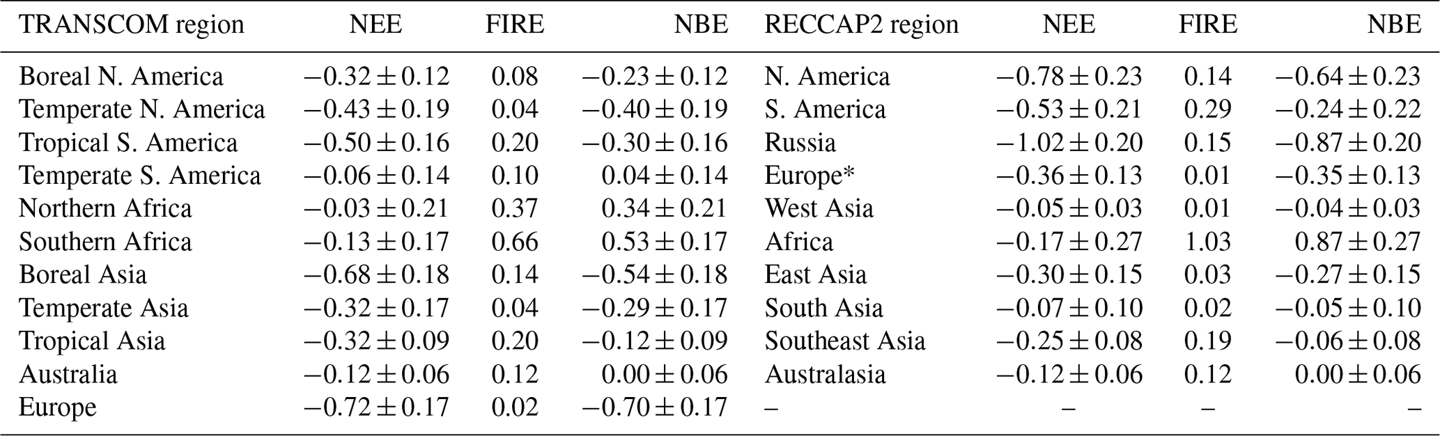
^* Excluding European Russia.

Table 2 lists the aggregated mean posterior annual NEE, NBE, and FIRE emissions during the 10 years for the 11 TRANSCOM regions and the 10 RECCAP2 regions. Compared with the prior NEE, the absolute relative changes in most TRANSCOM regions are greater than 50 % (Fig. S5) after being constrained with GOSAT data. In all regions, the aggregated posterior NEE is negative, indicating a carbon sink in each region. For the 11 TRANSCOM regions, we estimate that Europe has the strongest sink, followed by boreal Asia, tropical S. America, and northern Africa with the weakest sink. Among the 10 RECCAP2 regions, Russia's sink is the strongest, followed by N. America and Europe, and West Asia's sink is the weakest. It is worth noting that Europe's NEE in the TRANSCOM region is twice that in RECCAP2. This is because the coverage of Europe is different in TRANSCOM and RECCAP2; the former includes the entire European continent, while the latter does not include European Russia.

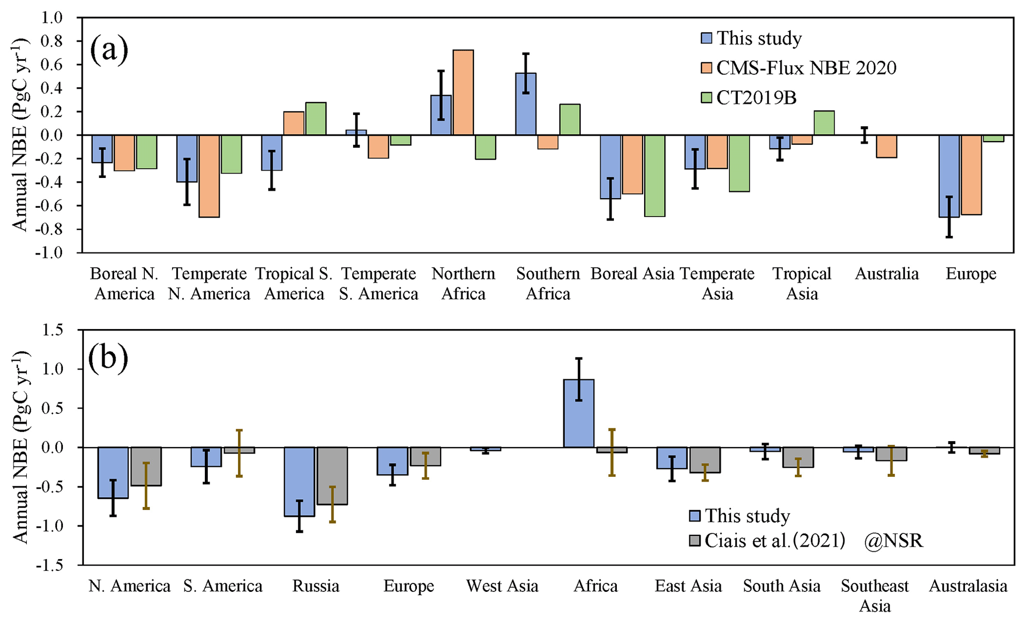
Figure 6 2010–2019 averaged regional NBE in (a) the TRANSCOM regions and (b) the RECCAP2 regions. Both CMS-Flux NBE 2020 and CT2019B are averaged from 2010 to 2018. The result of Ciais et al. (2021) is a bottom-up estimate, which is for the period of 2000–2009.

Figure 6 shows a comparison between the results of this study and previous studies for both the TRANSCOM and RECCAP2 regions. For the TRANSCOM region, as shown in Fig. 6a, in temperate N. America, northern Africa, and boreal Asia, the estimates of this study are between the results of CMS-Flux NBE 2020 and CT2019B; in temperate Asia, Europe, and tropical Asia, our estimates are very close to CMS-Flux but are significantly different with CT2019B. Conversely, in Australia, our estimates are very consistent with CT2019B but are significantly different from CMS-Flux. In tropical S. America, our result shows a strong carbon sink, which is consistent with previous mean annual biomass sink estimate of $-\mathrm{0.39}\pm \mathrm{0.10}$ PgC yr⁻¹ in the Amazon during the 1980–2004 period based on repeated censuses at a widespread forest plot network (Phillips et al., 2009) and is roughly consistent with a regional inversion in a wet year of −0.25 PgC yr⁻¹ based on aircraft CO₂ measurements (Gatti et al., 2014), while CMS-Flux NBE 2020 and CT2019B are both carbon sources. On the contrary, in temperate S. America, our result shows a weak carbon source, while the other two are both carbon sinks. In addition, in southern Africa, our estimate is also significantly different from them; we show a strong carbon source, while CMS-Flux NBE 2020 and CT2019B show a weak sink and source, respectively. The differences between this study and CMS-Flux NBE 2020 may be related to the different XCO₂ products used. As mentioned before, the NBEs of CMS-Flux from 2010–2014 and 2015–2018 were inferred from GOSAT and OCO-2 products, respectively. In general, OCO-2 XCO₂ has much better spatial coverage than GOSAT XCO₂. Wang et al. (2019) pointed out that data amount is one of the most important factors affecting the inversion results; generally, in one region with more XCO₂ data, the carbon flux relative to the prior flux changes more. Therefore, we conduct an additional comparison for the periods of 2010 to 2014 and 2015 to 2018, respectively, since in the first stage, the XCO₂ used in these two studies is almost the same (both GOSAT), while in the second stage, it is different. As shown in Fig. S6, except for southern Africa, the difference between the two is significantly smaller in 2010–2014 than in 2015–2018, especially in temperate S. America, northern Africa, and Australia, confirming that the significant differences are mainly from the different XCO₂ products used in these two studies. In addition to XCO₂ data, the prior carbon flux can also have a significant impact on the inversion results (Philip et al., 2019). We further examine the prior and posterior NBE over southern Africa in these two studies and find that the prior NBEs used in these two systems are quite different (a strong sink in CMS-Flux and a source in this study). In the first stage, the NBE changes (Δ_NBE; a posteriori minus a priori) due to the GOSAT constraints are quite small in both studies (Fig. S7), resulting in the large difference in the posterior NBE between these two studies, while in the second stage, because of the better spatial coverage of OCO-2 XCO₂, the Δ_NBE in CMS-Flux increases significantly, resulting in a shift of NBE from an a priori strong sink to an a posteriori medium source, thus reducing the difference of the posterior NBE in these two studies. We also find that there is also an increase in the Δ_NBE in this study, which may be related to the increase of GOSAT XCO₂ data from 2010 to 2019 (Taylor et al., 2022).

Based on inventory data of carbon-stock changes and satellite estimates of biomass changes where inventory data are missing, Ciais et al. (2021) gave a state-of-the-art estimate for the NBE of the RECCAP2 regions for the period of 2000–2009, which was calculated by taking the sum of the carbon-stock change and lateral carbon fluxes from crop and wood trade and riverine-carbon export to the ocean. Figure 6b shows a comparison between this study and Ciais et al. (2021). Although the inverted NBE is not completely equivalent to the land sink obtained by the bottom-up method, generally, to reconcile top-down and bottom-up results, the inverted NBE should be adjusted with the lateral transport of reduced carbon compounds (RCCs) and carbon release from net imported products (Ciais et al., 2008; Jiang et al., 2016). Overall, except for Africa and South Asia, the NBEs estimated in this study and Ciais et al. (2021) are comparable. In Africa, we show a strong carbon source of 0.87±0.27 PgC yr⁻¹, while Ciais et al. (2021) reported a very weak sink of $-\mathrm{0.07}\pm \mathrm{0.29}$ PgC yr⁻¹. Until now, there have still been big differences in top-down estimates of African NBE in different studies. Generally, the estimates based on surface CO₂ measurements show carbon sinks or a weak source, which are mainly in the range of −0.26 to 0.32 PgC yr⁻¹ (Valentini et al., 2014; Jacobson et al., 2020), while the estimates from satellite XCO₂ retrievals report strong carbon sources, with values mainly in the range of 0.61 to 2.2 PgC yr⁻¹ (Liu et al., 2021; Palmer et al., 2019). Peiro et al. (2022) also found a similar phenomenon by comparing the carbon fluxes constrained using in situ observations and OCO-2 retrievals within the same inversion frameworks. Although the estimates based on surface measurements are much closer to the result of Ciais et al. (2021), the surface CO₂ observation sites in Africa are very sparse; there are only four stations over the African continent and two stations located in adjacent islands, indicating that the constraints from surface measurements are very poor, and the inverted fluxes often reflect the prior fluxes used in these inversions (Valentini et al., 2014). In our prior flux, the NBE in Africa is 0.34 PgC yr⁻¹, which is consistent with above surface-based estimates. This indicates that the strong carbon source is almost constrained from satellite XCO₂. Since there is no TCCON site in Africa, which is usually used to verify and correct the satellite XCO₂ retrievals, there are larger uncertainties in the XCO₂ products, thus probably resulting in an overestimation of the surface flux. Peiro et al. (2022) reported that the version of OCO-2 retrievals had a significant effect on the inversion results in Africa. However, due to the lack of validation data for XCO₂ and few in situ CO₂ measurements, it is hard to know for sure which is more accurate. In South Asia, we show a very weak sink of $-\mathrm{0.05}\pm \mathrm{0.10}$ PgC yr⁻¹, while Ciais et al. (2021) presented a moderate sink of −0.25 PgC yr⁻¹. Based on bottom-up and top-down methods, there have been many studies on NBE in South Asia in the past. Overall, the bottom-up estimates are in the range of −0.01 to −0.25 PgC yr⁻¹ (Cervarich et al., 2016; Ciais et al., 2021; Nayak et al., 2015; Gahlot et al., 2017; Patra et al., 2013), while the top-down estimates are in the range of 0.04 to −0.37 PgC yr⁻¹ (Patra et al., 2013; Thompson et al., 2016; Cervarich et al., 2016; Niwa et al., 2012; Jiang et al., 2014; Swathi et al., 2021). Our result for South Asia is in the range of these previous studies.

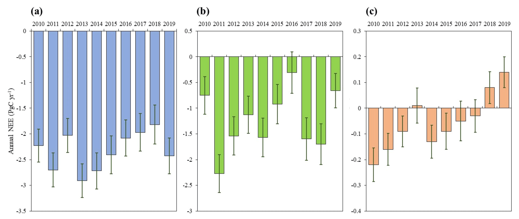
Figure 7 Interannual variations of annual NEE of different latitudes (a northern midlatitudes to high latitudes (>30^∘ N); b tropical latitudes (30^∘ S–30^∘ N); c southern middle latitudes (<30^∘ S)).

5.3 Interannual variations and seasonal cycles

Figure 7a, b, and c show interannual variations (IAV) of the NEE in the NL, TL, and SL, respectively. In NL, the IAV of NEE is relatively small, with an interannual amplitude of 1.09±0.50 PgC yr⁻¹. The smallest year of NEE appeared in 2018, which was $-\mathrm{1.87}\pm \mathrm{0.38}$ PgC yr⁻¹, and the largest year appeared in 2014, with a value of $-\mathrm{2.91}\pm \mathrm{0.33}$ PgC yr⁻¹. In TL, the inter-annual variability is very large, with the biggest NEE in 2011 of $-\mathrm{2.27}\pm \mathrm{0.33}$ PgC yr⁻¹ and the smallest NEE in 2016 only $-\mathrm{0.31}\pm \mathrm{0.41}$ PgC yr⁻¹. The interannual amplitude of NEE in TL is nearly twice that of NL, which reaches 1.96±0.53 PgC yr⁻¹. The strongest carbon sink in 2011 and weakest sink in 2016 are related to the strongest 2011 La Niña and 2015/2016 El Niño events, respectively, which is in good agreement with many previous findings (Liu et al., 2017; Bastos et al., 2018; Wang et al., 2018; Koren et al., 2018). Bastos et al. (2018) showed a smaller difference of carbon fluxes between 2015 and 2011 using both bottom-up and top-down approaches, which was in the range of 0.7–1.9 PgC yr⁻¹. With the constraints of GOSAT and OCO-2 XCO₂, Liu et al. (2017) found that relative to the 2011 La Niña, the pantropical biosphere released 2.5±0.34 PgC more carbon into the atmosphere in 2015, and during the peak 2015–2016 El Niño between May 2015 and April 2016, the released carbon reached 3.3±0.34 PgC. In this dataset, the changes of carbon flux between 2011 La Niña and 2015–2016 El Niño events in the pantropical area are lower than the estimates of Liu et al. (2017) but close to Bastos et al. (2018). We estimate that the change of NBE between 2015 and 2011 is 1.59±0.34 PgC yr⁻¹, and the peak period of 2015–2016 El Niño released 2.79 PgC more than in 2011 (Fig. S8). In addition, it also could be found that there are weak carbon sinks in 2010 and 2019 in TL. There have been many studies on the decline of carbon sinks in tropical regions in 2010 (van der Laan-Luijkx et al., 2015; Doughty et al., 2015; Gatti et al., 2014). In 2019, the decrease of NEE may be related to the Indian Ocean Dipole event, which significantly reduced the carbon uptakes over southern China, the former Indo-China peninsula, and Australia (Wang et al., 2021b). In SL, due to the small land area, its NEE is an order of magnitude lower than the other two regions. It could be found that there is a continuous decreasing trend. This trend is basically consistent with that in Australia (Fig. 8j), indicating that the IAV of NEE in SL is dominated by that in southern Australia, especially in southeastern Australia (Byrne et al., 2021). Previous studies have revealed that the enhanced carbon uptake in Australia from 2010 to 2012 was associated with the La Niña phase from the end of 2010 to early 2012 (Detmers et al., 2015), while the significantly increased carbon loss in 2019 was due to extreme drought (Byrne et al., 2021) associated with the Indian Ocean Dipole event (Wang et al., 2021b), indicating that the decreasing trend of carbon sink in SL is caused by the extreme climate events that occurred in the start and end years of this decade, respectively; thus this downtrend is just a coincidence. On average, the NEEs in NL, TL, and SL during this decade are $-\mathrm{2.33}\pm \mathrm{0.35}$, $-\mathrm{1.25}\pm \mathrm{0.38}$, and $-\mathrm{0.05}\pm \mathrm{0.07}$ PgC yr⁻¹, which account for 62.6 %, 33.4 %, and 1.4 % of the global total land sink, respectively, indicating that the global land NEE is dominated by the NEE in NL. However, the correlation coefficients between the IAVs of NEE in these three regions (NL, TL, and SL) and the IAV of global terrestrial NEE are 0.57, 0.86, and 0.37, respectively, indicating that the IAV of global NEE is dominated by its inter-annual changes in TL.

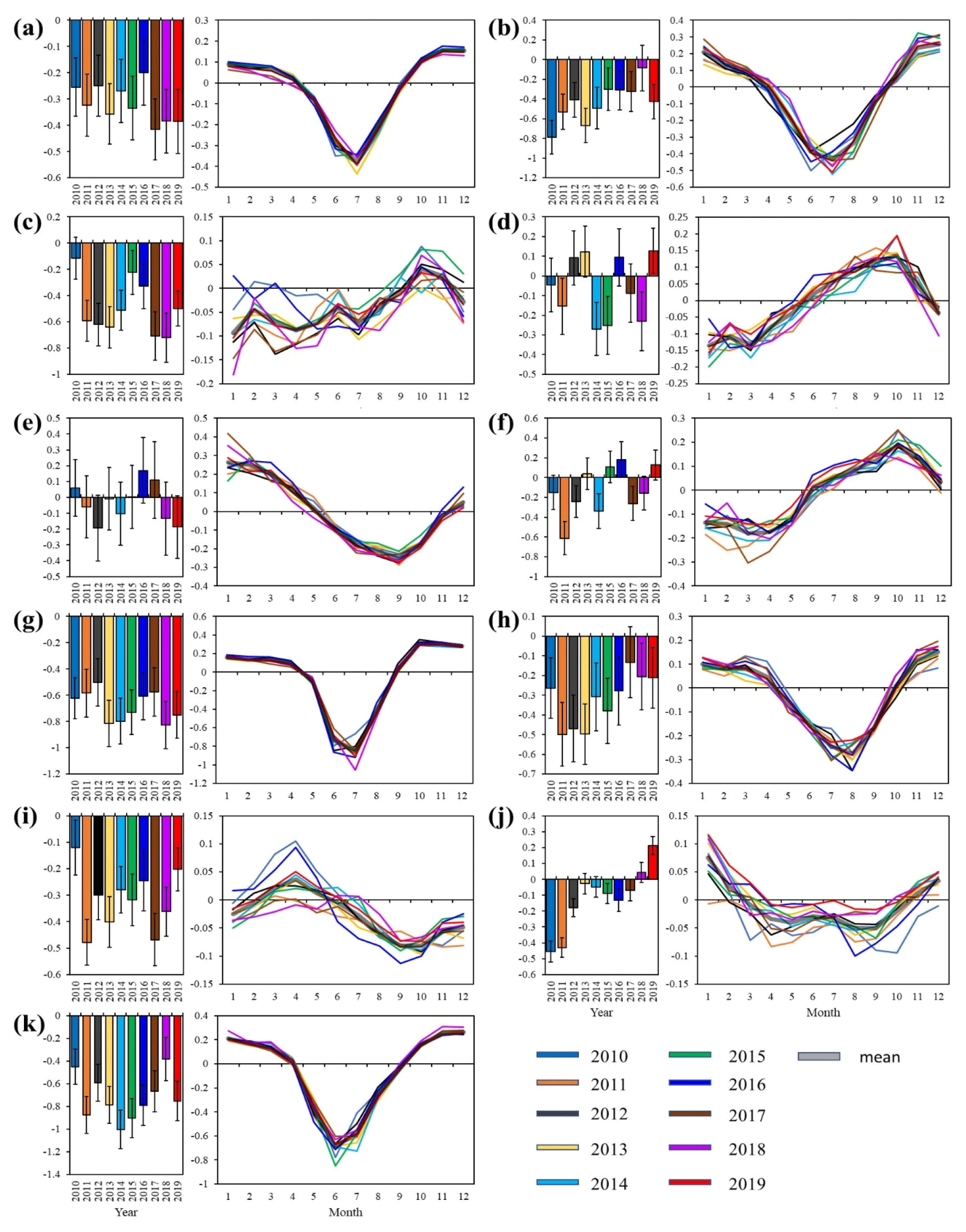
Figure 8 Interannual variations of the annual (unit: PgC yr⁻¹) and monthly (unit: PgC per month) NEE in the 11 TRANSCOM regions (a boreal N. America; b temperate N. America; c tropical S. America; d temperate S. America; e northern Africa; f southern Africa; g boreal Asia; h temperate Asia; i tropical Asia; j Australia; k Europe).

In Fig. 8, we further present the IAVs and seasonal cycles of NEE in the 11 TRANSCOM regions. Since there are some overlaps between the TRANSCOM and RECCAP2 regions, for example, the N. America region in RECCAP2 is almost the sum of the boreal and temperate N. America, and the Africa region in RECCAP2 is the sum of northern and southern Africa in TRANSCOM. In addition, the IAVs of NEE in some regions of RECCAP2 like Russia and East Asia are dominated by the NEE changes in corresponding regions in TRANSCOM. Therefore, here we only analyze the annual and monthly changes of NEE in the TRANSCOM regions. The differences for the IAVs between the prior and posterior NEE in each region are shown in Fig. S9.

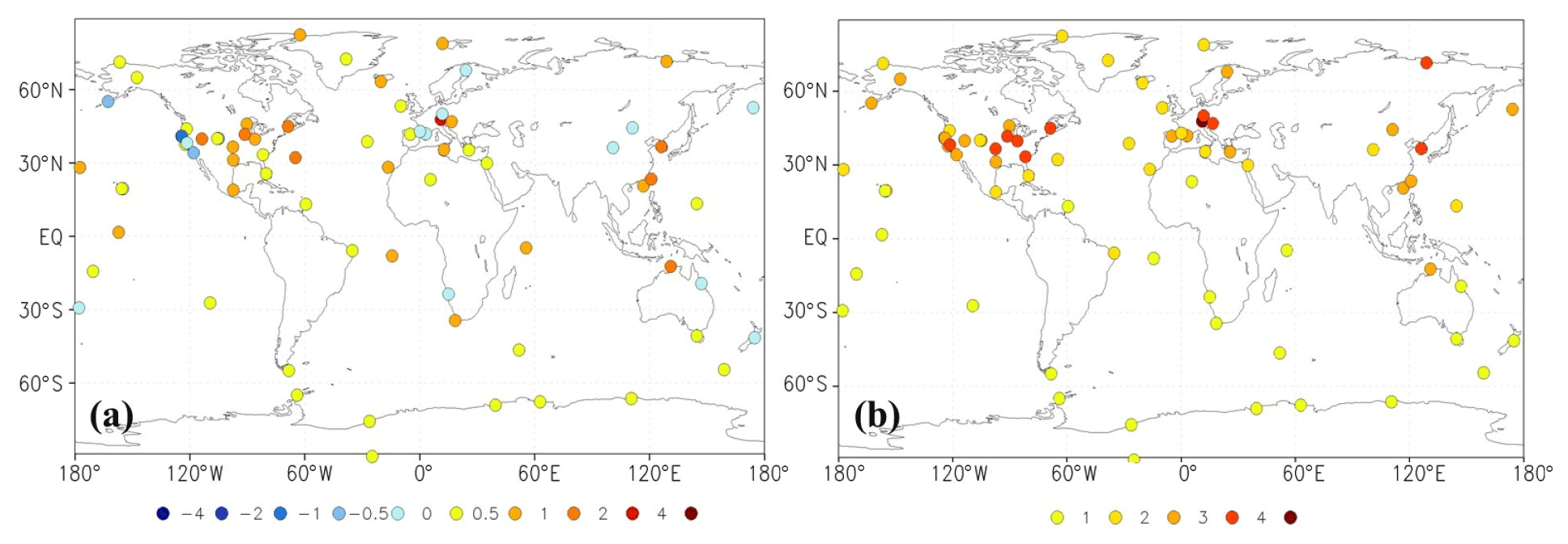
Figure 9 Spatial distributions of the (a) BIAS and (b) MAE of the posterior CO₂ concentrations at each site (simulations minus observations; unit: ppm).

There are significant differences in the IAVs of annual NEE in each region. For example, in boreal N. America, the weakest sink is in 2016 and the strongest sink in 2017, while in temperate N. America, the weakest sink occurs in 2018 and the strongest in 2010. Europe has the weakest sink in 2018, but the strongest sink is in 2014. For the interannual amplitudes, temperate N. America, tropical S. America, southern Africa, Australia, and Europe have relatively larger interannual amplitudes, with values above 0.6 PgC yr⁻¹. In temperate S. America, boreal Asia, northern Africa, temperate Asia, and tropical Asia, the interannual amplitudes are comparable, ranging from 0.33 to 0.40 PgC yr⁻¹, while boreal N. America has the smallest interannual amplitude of 0.22 PgC yr⁻¹. Except for boreal N. America, boreal Asia, and Europe, the interannual amplitudes in other regions are larger than their 10-year averaged carbon sinks, especially in temperate S. America, northern and southern Africa, and Australia; their inter-annual amplitudes of NEE reach more than 5 times of the mean carbon sinks.

For the seasonal cycles, the northern middle- and high-latitudinal regions have a similar pattern, with carbon sources during the cold season (from October to April) and carbon sinks during the warm season (from May to September). In the cold season, the difference of carbon releases in different regions is relatively small, but in the warm season, the intensity of carbon sinks in different regions is significantly different, and the months in which the strongest carbon sinks appear are also different. Boreal Asia and temperate and boreal N. America have the strongest sinks in July, and Europe has the strongest one in June, while temperate Asia has the strongest in August. For the southern lands, southern Africa and temperate S. America have a similar seasonal cycle. Their carbon sources occur from July to about December, with a peak in October, and carbon sinks appear from January to May. In Australia, the carbon sinks mainly occur from March to October. In the tropics, northern Africa has an opposite seasonal cycle to its adjacent region of southern Africa; its carbon sink occurs during June to November. The seasonal cycles in tropical Asia and tropical S. America are also nearly opposite. Tropical Asia has the strongest sink in September and October, while tropical S. America has the strongest carbon release in October. In general, the tropical regions have a smaller seasonal amplitude, while the high latitudes have a larger seasonal amplitude. The seasonal amplitudes in boreal Asia and Europe reach 1.17 and 0.96 PgC per month, respectively, while in tropical Asia and tropical S. America, the seasonal amplitudes are only about 0.12 PgC per month. The same region has basically similar seasonal cycles in different years, but the intensity of its carbon sources and sinks, the time of transition from carbon source to carbon sink, and the months with the strongest sink or source are also significantly different in different years. For example, in tropical Asia, the carbon sources from January to April in 2010 and 2016 are significantly stronger than those in normal years; in temperate N. America, the carbon sinks in the spring of 2012 are significantly stronger than normal, but the carbon sinks in the summer are significantly weaker than normal.

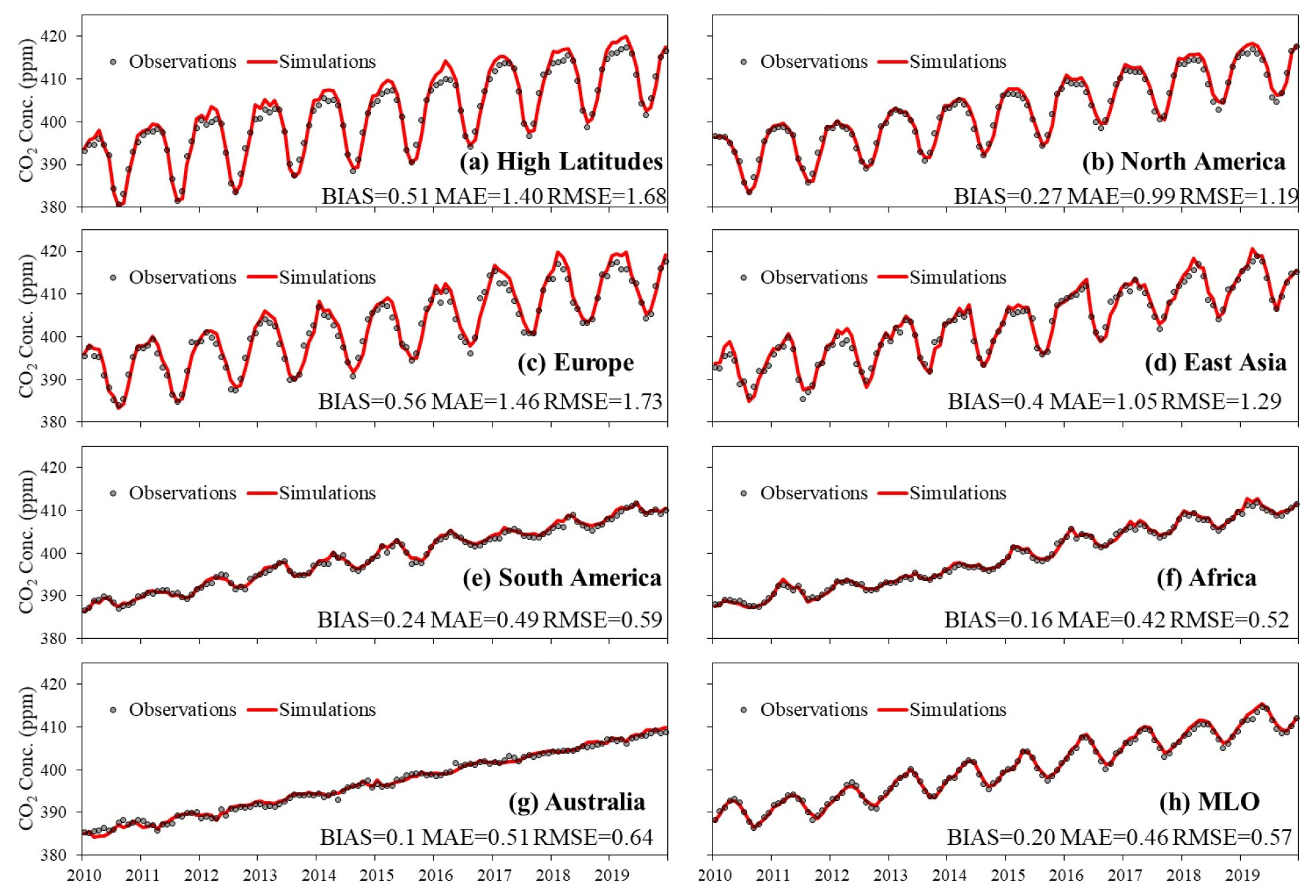
Figure 10 Time series of monthly averaged observations and simulations in the seven regions and at the MLO site.

Generally, the IAVs of annual NEE and seasonal cycles are related to large-scale climate anomalies and regional extreme climate events like droughts, heat waves, and precipitation, which have been widely studied around the world (e.g., Ciais et al., 2005; Betts et al., 2020; Bastos et al., 2018; Koren et al., 2018; Reichstein et al., 2013; Frank et al., 2015; Zhao and Running, 2010). Evidence has shown that severe drought events that occurred in the Amazon in 2010 (Potter et al., 2011; Doughty et al., 2015), Europe in 2010 (Bastos et al., 2020a), 2012 (He et al., 2019), and 2018 (Bastos et al., 2020b; Graf et al., 2020; Wang et al., 2020), the United States in 2011–2012 (He et al., 2018; Wolf et al., 2016; Liu et al., 2018; Byrne et al., 2020) and 2018 (Li et al., 2020), and Australia in 2019 (Byrne et al., 2021) caused significant reductions of terrestrial carbon uptakes. Accordingly, as shown in Fig. 8, the NEEs in this dataset are also much smaller in those years and regions compared with the normal year. In particular, in 2012, the contiguous United States experienced exceptionally warm temperatures and the most severe drought since the Dust Bowl era of the 1930s. Wolf et al. (2016) found that the warm spring reduced the impact of the summer drought on net annual carbon uptake across the United States. As mentioned above, our dataset also shows the significant increase of carbon sink in the spring of 2012 and a large decrease during the summertime in temperate N. America. In summer 2010, western Russia was hit by an extraordinary heat wave, with the region experiencing by far the warmest July since records began (Otto, et al., 2012; Guerlet et al., 2013; Ishizawa et al., 2016); correspondingly, we find that in our dataset, the carbon sink in boreal Asia in July 2010 is the weakest in this decade, and the areas with a significant positive anomaly of NEE (source increase) are mainly in western Russia (Fig. S10). The strong El Niño events in 2015 and 2016 led to a significant reduction in carbon sinks in the pantropical regions, and many regions even turned to carbon sources (Liu et al., 2017; Bastos et al., 2018). Clearly, during 2015–2016, the inverted carbon sink in this study is much weaker than normal years in tropical S. America and tropical Asia, and it turns to carbon sources in northern and southern Africa. These indicate that this NEE dataset could clearly reveal the impact of climate extremes on carbon uptakes; thus it will be of benefit for studies of the trends and drivers of carbon flux in different regions of the world.

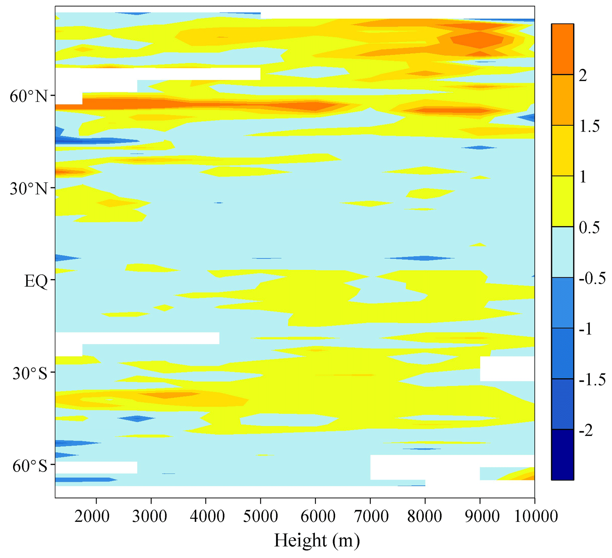
Figure 11 Statistical results for monthly mean profiles in the eight Asia-Pacific cities (a Hong Kong, b Bangkok, c Singapore, d Jakarta, d Tokyo, f Shanghai, g New Delhi, and h Sydney).

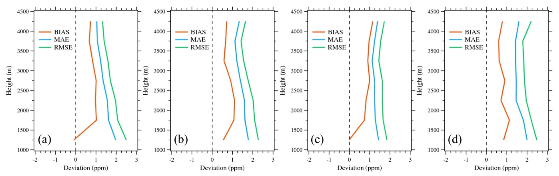
Figure 12 Statistical results at different heights against the observations in the Amazon basin (a ALF; b RBA; c SAN; d TAB_TEF).

Figure 13 BIAS at different latitudes and heights against the HIPPO observations.

6 Evaluations

6.1 Against surface flask observations

As shown in Sect. 3, surface flask observations from 74 sites are used to evaluate the inversion results. The modeled CO₂ concentrations were extracted from the simulated 3 h interval 3-D CO₂ fields according to the locations, time, and heights of each observation. It should be noted that the records with absolute biases between the posterior CO₂ concentrations and CO₂ measurements greater than 10 ppm were removed, which are considered to have a lack of regional representativeness. Due to the low spatial resolution ($\mathrm{1.9}{}^{\circ }\times \mathrm{2.5}{}^{\circ }$) of our model, we cannot reproduce such observations. Figure 9 shows the comparisons between the posterior CO₂ concentrations and surface flask CO₂ measurements. At most sites located in ocean areas, tropical lands, and southern lands, the BIAS is within ±0.5 ppm, and MAE is lower than 1 ppm. In the northern midlatitudes to high latitudes, BIAS of some stations is higher than ±1.0 ppm, and MAE of almost all stations is higher than 1.5 ppm (Table S1). The global mean BIAS, MAE, and RMSE are 0.36, 1.76, and 2.28 ppm. The CORR of each site is in the range of 0.86 and 1, with a global mean of 0.96.

The higher deviations in the northern midlatitudes to high latitudes, especially in temperate N. America and Europe, are probably due to the mismatch of spatial and temporal representativeness between the observations and simulations. In order to further increase the spatial and temporal representativeness of the observations, regional and monthly mean observed and modeled concentrations in seven land regions are compared. As shown in Fig. 1, the seven regions are high latitudes (>60^∘ N), N. America, S. America, Europe, East Asia, Africa, and Australia. There are 8 sites in the high latitudes, 19 sites in N. America, 9 sites in Europe, 5 sites in East Asia, 3 sites in S. America, 5 sites in Africa, and 4 sites in Australia (Fig. 1, Table S1). Figure 10 shows the time series of the monthly observed and modeled CO₂ concentrations in the seven regions. In addition, the Mauna Loa Observatory (MLO) in Hawaii is a global background site; the comparisons of monthly mean concentrations at MLO are also shown in Fig. 10. Clearly, the modeled regional and monthly mean CO₂ concentrations agree well with the observations. The mean BIAS values are in the range of 0.1 to 0.56 ppm, and MAE and RMSE are in the range of 0.42–1.46 and 0.52–1.73 ppm, respectively. In S. America, Africa, and Australia, the posterior CO₂ concentrations are very consistent with the observations, with BIAS only in the range of 0.1–0.24 ppm, and MAE about 0.5 ppm. Among these regions, the deviations in Europe and high-latitude regions are relatively larger, with a MAE of greater than 1.4 ppm and a RMSE about 1.7 ppm. Significant positive biases mainly occur during the winter. This is understandable because in the winter at high latitudes, satellite observations are very scarce, leading to very insufficient constraints on the winter carbon flux. This indicates that there may be an overestimation of carbon releases at high latitudes in winter. At MLO, the simulations also agree well with the observations, with BIAS, MAE, and RMSE of 0.2, 0.46, and 0.57 ppm, respectively. Figure S11 shows the time series of biases in the seven regions and at the MLO site; for comparison, the biases of prior CO₂ concentrations are also shown in this figure. Clearly, the biases of the simulated CO₂ concentrations are significantly decreased relative to the prior. It also could be found that there is an upward trend in the biases of the posterior CO₂ concentrations in all regions except East Asia, as well as at the MLO site. On global average (74 sites), the annual mean biases increase from −0.36 ppm in 2010 to 0.75 ppm in 2019, with an uptrend slope of 0.115 ppm yr⁻¹ (Fig. S12). By multiplying by a factor of 2.124 PgC ppm⁻¹ (Ballantyne et al., 2012), this bias accumulation rate is equal to 0.244 PgC yr⁻¹, which is very consistent with the 10-year-averaged bias in the inverted global AGR given in Sect. 5.1 (0.25 PgC yr⁻¹). This uptrend is a result of a residual trend in the inversions fit to the GOSAT data. We analyze the time series of the global averaged monthly mean posterior XCO₂ and GOSAT XCO₂ concentrations and find that the mismatches between the posterior XCO₂ fields and GOSAT data also have an upward trend from 2010 to 2019, with an annual mean increment about 0.09 ppm yr⁻¹ (Fig. S13).

6.2 Against aircraft measurements

We further evaluate the posterior CO₂ concentrations against the aircraft observations. First, the posterior CO₂ were extracted from the simulated CO₂ fields according to the locations, time, and heights of each aircraft observation, and then, both the observed and modeled CO₂ concentrations were divided into 14 layers: 1000–1500, 1500–2000, 2000–2500, 2500–3000, 3000–3500, 3500–4000, 4000–4500, 4500–5000, 5000–5500, 5500–6000, 6000–7000, 7000–8000, 8000–9000, and above 9000 m (CONTRAIL only 3–10 layers and CARBAM only 1–8 layers). Monthly mean observed and modeled CO₂ concentrations at each height were calculated and compared for the CONTRAIL and CARBAM profiles. For comparisons against the HIPPO observations, the data were further divided into 2^∘ intervals along the longitudinal direction, and all data in each layer and 2^∘ latitudinal intervals were averaged.

Figures 11 and 12 show the evaluation results of monthly mean profiles in eight cities over the Asia-Pacific region and at four sites in the Amazon basin, respectively. Overall, the deviations between the simulations and observations decrease with height. In the Asia-Pacific region, the BIAS is basically within ±0.5 ppm, and most MAE values are smaller than 1 ppm, especially in Southeast Asia, indicating that we have a good estimate of NEE in this area. Shanghai and New Delhi have relatively larger MAE and RMSE values, with MAE about 1.5 ppm and RMSE existing 2 ppm in the lowest level, probably due to the fact that Shanghai and New Delhi are one of the largest cities in China and India, respectively, and have very strong anthropogenic CO₂ emissions, which may affect the performance of the MOZART model. In the Amazon basin, the MAE and RMSE of all four sites decrease with height, with MAE and RMSE decreasing from about 2 ppm near 1000 m height to about 1.5 ppm near 4000 m. For BIAS, below 2000 m, they increase significantly with height. There are negative ($\sim -\mathrm{1.0}$ ppm, data not shown), small (∼0.2 ppm), and significant positive BIAS (∼0.9 ppm) values below 1000 m, at 1000–1500 m, and at 1500–2000 m height, respectively, indicating that there are considerable vertical transport errors, and the carbon sinks over tropical S. America may have systematic biases.

Figure 13 shows the comparisons against the HIPPO observations at different heights and latitudes. Overall, most BIAS values are within ±0.5 ppm, showing a good agreement between the simulations and observations. Relatively large BIAS occurs over northern high latitudes, which is consistent with the comparisons against the surface observations as shown in Fig. 10 and also reveals an overestimation of carbon releases at high latitudes.

7 Data availability

The GCAS2021 data are available at https://doi.org/10.5281/zenodo.5829774 (Jiang, 2022). The regional aggregated fluxes are provided as .xlsx files with a file size of ∼135 KB, and the gridded fluxes and ensemble members are provided in NetCDF format with a file size ∼82 MB and 5.8 GB, respectively.

8 Summary

A global NEE dataset is essential for estimating the regional terrestrial carbon budget and understanding the responses of carbon fluxes to extreme climates. Here, by assimilating the GOSAT ACOS v9 XCO₂ product, we generate a 10-year global monthly terrestrial NEE dataset from 2010 to 2019 (GCAS2021) using the GCASv2 system. GCAS2021 includes monthly and annual gridded ($\mathrm{1}{}^{\circ }\times \mathrm{1}{}^{\circ }$) prior and posterior NEE and OCN flux, prescribed FIRE and FFC emissions, and globally, latitudinally, and regionally aggregated fluxes and their uncertainties. Globally, the decadal mean NBE and AGR as well as their IAVs match well with the estimates of GCP2020. Regionally, our product shows carbon sinks over eastern N. America, the Amazon, the Congo Basin, Europe, boreal forests, southern China, and Southeast Asia and carbon sources over the western United States, African grasslands, Brazilian plateau, and parts of South Asia. In the 11 TRANSCOM land regions, the NBEs of temperate N. America, northern Africa, and boreal Asia are between the results of CMS-Flux NBE 2020 and CT2019B, and those in temperate Asia, Europe, and tropical Asia are very close to CMS-Flux NBE 2020 but significantly different from CT2019B. In the RECCAP2 regions, except for Africa and South Asia, the NBEs are comparable with the latest bottom-up estimate of Ciais et al. (2021). The IAVs and seasonal cycles of NEE could clearly reflect the impact of extreme climates or large-scale climate anomalies. We also qualitatively evaluate the NEE estimates by comparing posterior CO₂ concentrations with independent CO₂ measurements from surface flask and aircraft CO₂ observations, and the results show that the simulated remote site and regional average CO₂ concentrations, as well as the vertical CO₂ profiles, are all consistent with the observations. We believe that this dataset will be useful in the estimates of regional- or national-scale terrestrial carbon budgets, the study of carbon sink evolution mechanisms, the evaluation of ecosystem models, and the assessments of carbon neutrality strategies.