the Creative Commons Attribution 4.0 License.
the Creative Commons Attribution 4.0 License.
 | 12 May 2022
A global drought dataset of standardized moisture anomaly index incorporating snow dynamics (SZIsnow) and its application in identifying large-scale drought events
Lei Tian
Baoqing Zhang
Pute Wu
Drought indices are hard to balance in terms of versatility (effectiveness for multiple types of drought), flexibility of timescales, and inclusivity (to what extent they include all physical processes). A lack of consistent source data increases the difficulty of quantifying drought. Here, we present a global monthly drought dataset with a spatial resolution of 0.25∘ from 1948 to 2010 based on a multitype and multiscalar drought index, the standardized moisture anomaly index incorporating snow dynamics (SZIsnow), driven by systematic fields from an advanced data assimilation system. The proposed SZIsnow dataset includes different physical water–energy processes, especially snow processes. Our evaluation of the dataset demonstrates its ability to distinguish different types of drought across different timescales. Our assessment also indicates that the dataset adequately captures droughts across different spatial scales. The consideration of snow processes improved the capability of SZIsnow, and the improvement is particularly evident over snow-covered high-latitude (e.g., Arctic region) and high-altitude areas (e.g., Tibetan Plateau). We found that 59.66 % of Earth's land area exhibited a drying trend between 1948 and 2010, and the remaining 40.34 % exhibited a wetting trend. Our results also indicate that the SZIsnow dataset can be employed to capture the large-scale drought events that occurred across the world. Our analysis shows there were 525 drought events with an area larger than 500 000 km2 globally during the study period, of which 68.38 % had a duration longer than 6 months. Therefore, this new drought dataset is well suited to monitoring, assessing, and characterizing drought and can serve as a valuable resource for future drought studies. The database is available at http://doi.org/10.5281/zenodo.5627369 (Wu et al., 2021).
- Article
(13186 KB) - Full-text XML
-
Supplement
(3189 KB) - BibTeX
- EndNote


Drought is one of the most costly and complex natural hazards, commonly causing significant and widespread adverse impacts on many sectors of society (Aghakouchak et al., 2015; He et al., 2020). The severity, extent, and duration of drought are likely to intensify across the world under the effects of climate change (Ault, 2020; Mann and Gleick, 2015). There has been increasing global interest in measures to improve the capability of drought quantification, and various drought indices have been proposed over the past several decades (Liu et al., 2018; Esfahanian et al., 2017; Zhang et al., 2021). However, current drought indices struggle to reconcile versatility (ability to quantify multiple types of drought), flexibility of temporal scale (effective across different timescales), and comprehensiveness (to what extent they include all hydrological processes). Additionally, these drought indices are derived from multifarious data sources, rather than systematic and consistent physical data from the same source (Ahmadalipour and Moradkhani, 2017; Hoffmann et al., 2020; Zheng et al., 2019). As a result, different sectors of society have rarely collaborated to synergistically fight against drought using a comprehensive drought index.
The propagation of drought is related to changes in numerous interconnected variables of hydrometeorological processes (e.g., precipitation, evapotranspiration, streamflow, and soil moisture). Yet a major portion of currently available drought indices focus on only one aspect of drought evolution. For example, the rainfall anomaly index (RAI; Zhu et al., 2021), streamflow drought index (SDI; Nalbantis and Tsakiris, 2009), and soil moisture deficit index (SMDI; Narasimhan and Srinivasan, 2005) focus only on precipitation (meteorological drought), streamflow (hydrological drought), and soil moisture (agricultural drought), respectively (Fig. 1, top row). Additionally, these indices merely consider water supply in drought and neglect water demand, but a drought is a condition of the water deficit between water supply and demand (Mishra and Singh, 2010). Thus, these indices do not provide sufficient information to enable decision-makers to organize a comprehensive anti-drought approach that balances all sectors of society affected by drought.
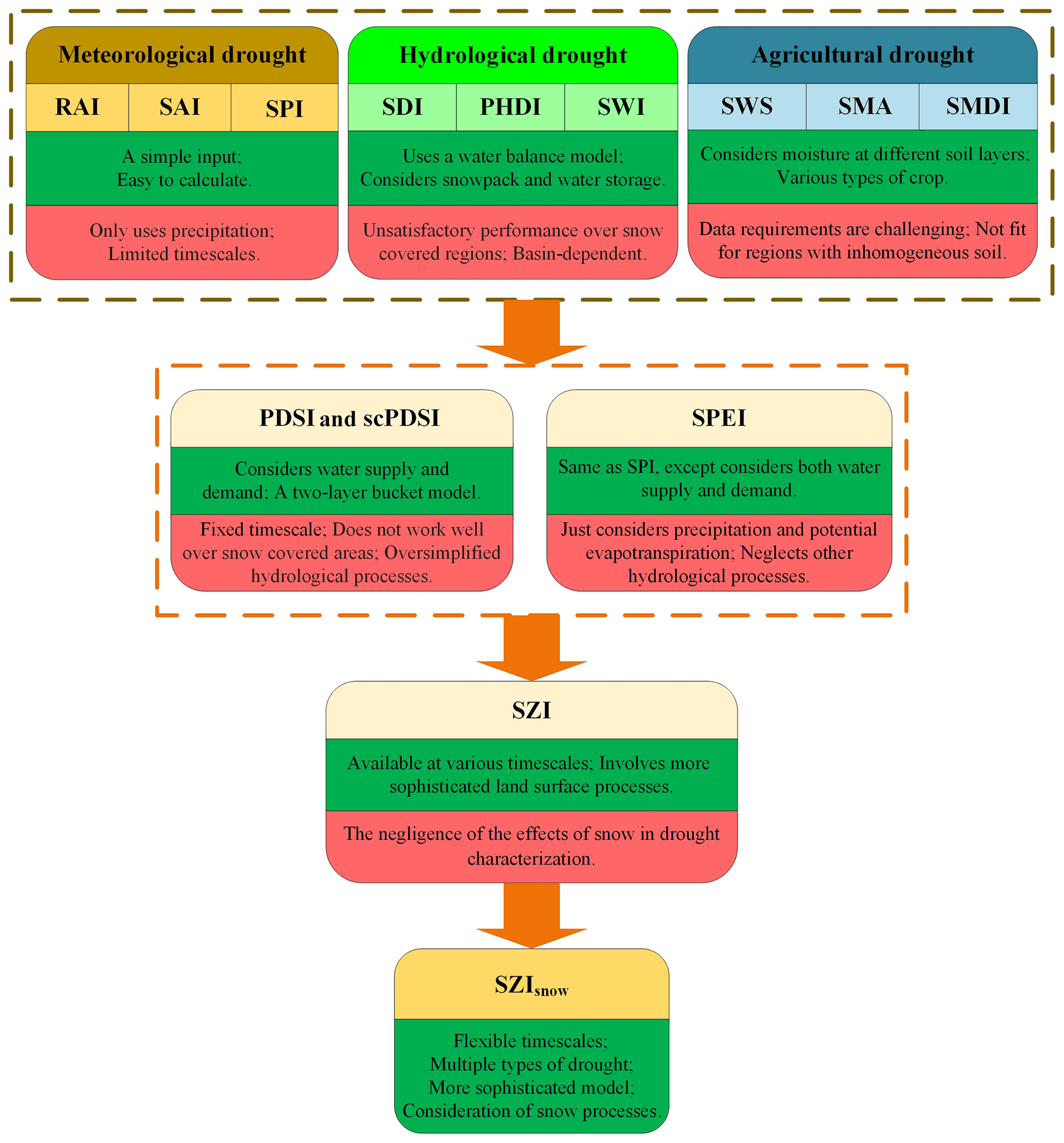
Figure 1Development path of the SZIsnow. Dark green boxes denote the strengths of each drought index, while pink boxes denote the weaknesses of each drought index. The top row shows indices that can only account for one type of drought, with three indices listed for each type of drought. The second row shows indices that can account for multiple types of drought. Full names of the listed indices are shown in Table S1 in the Supplement.
Some indices were developed with the purpose of application to all types of droughts (Fig. 1, second row). The Palmer drought severity index (PDSI; Alley, 1984; Wells et al., 2004) can be applied to different types of drought by considering water supply and demand with a simplified two-layer bucket model, but it has a fixed temporal scale and does not work well over snow-covered areas (Dai, 2011a). In addition, the self-calibrated PDSI (scPDSI) can dynamically compute the constants in PSDI on the basis of the characteristics at each interested location, producing more representative model constants. However, the scPDSI has the same issues as the PDSI in terms of the temporal scale and performance over snow-covered areas. Although the standardized precipitation evapotranspiration index (SPEI; Vicente-Serrano et al., 2010) overcomes the PDSI's weakness of fixed temporal scale, it oversimplifies complex relationships and neglects several important hydrological processes associated with the development of drought (Zhang et al., 2015). Moreover, current indices usually use physical variables from different data sources, which inevitably introduces bias and leads to an imbalanced calculation (Naumann et al., 2014). The development of the data assimilation system brings an option of systematic input for drought indices (Xu et al., 2020). Therefore, there is a need to develop a multitype and multiscalar drought index that considers various key processes related to drought and can take full advantage of output from the data assimilation system.
Given the abovementioned deficiency of current drought indices, Zhang et al. (2015) proposed a universal drought index, the standardized moisture anomaly index (SZI), to determine and monitor different types of droughts (Fig. 1, third row). Absorbing the strengths of the SPEI and PDSI, the SZI is available at flexible temporal scales and involves relatively sophisticated land surface processes. It builds a bridge between drought monitoring and the data assimilation system. In the SZI, the atmospheric water demand is calculated by using variables related to evapotranspiration, runoff, soil moisture infiltration, and soil moisture loss, while water supply is taken as actual precipitation. Thus, the difference between water supply and atmospheric water demand is used to scale the water deficit and surplus. Additionally, there are two main limitations of the SZI. The first one is that its computation is more difficult than the standardized precipitation index (SPI) or SPEI. Another limitation is that it needs a long-term serial of hydrometeorological records, making it unsuitable for short-term drought studies. Although the SZI has been evaluated and achieved acceptable performance, it ignores the effects of snow in drought characterization, similar to the PDSI and SPEI. Such negligence in the SZI can impair its capability to monitor and identify droughts, particularly for those snow-covered regions with considerable amounts of snowfall (Huning and Aghakouchak, 2020; Staudinger et al., 2014). To address this deficiency, Zhang et al. (2019) modified the SZI by adding snow dynamics for drought characterization into a new version of the drought index called SZIsnow (Fig. 1, final row). This is the drought index used to construct the drought dataset in this study.
Drought is mainly characterized by severity, spatial extent, duration, and timing. The traditional method for drought investigation is to explore the variability of its severity over a fixed study area (Hao et al., 2017). This method is also widely used to evaluate the ability of a drought index (Peng et al., 2020). Although this method can provide certain information regarding the regional drought condition, it cannot analyze the change of spatial extent with time for a drought event (Zhai et al., 2017). As drought is a spatiotemporal process, the ability of a drought index to explore the joint evolution of drought events in space and time should be given increased attention (Herrera-Estrada et al., 2017). Thus, we utilized the severity–area–duration method (Andreadis et al., 2005; Sheffield et al., 2009), which can monitor drought in space and time, to comprehensively evaluate the drought index dataset proposed by our work.
This work aims to construct a long-term global SZIsnow dataset for various temporal scales. The SZIsnow is here developed to characterize multitype and multiscalar drought by accounting for different physical water–energy processes, especially snow processes. This paper is organized as follows. We first introduce the data and metrics for forcing and evaluation of the proposed drought dataset (Sect. 2). The method behind the derivation of the SZIsnow is summarized in Sect. 3. In Sect. 4 we present a comprehensive evaluation of the SZIsnow to assess its ability to capture different drought types across the world, particularly over the Arctic region and Tibetan Plateau. Based on the dataset, we further analyze the spatiotemporal changes of global drought and focus on the variability of large-scale drought events. Section 5 briefly introduces how to download the proposed drought index dataset. Finally, in Sect. 6, we discuss the advancement of the SZIsnow and its potential applicability and implications, and we present our conclusions.
2.1 Data for producing the SZIsnow drought index
Hydrometeorological variables from numerical models are commonly used as the source data to compute drought indices at the global scale, due to limited observational data (Sawada and Koike, 2016). Thus, in this study, the Global Land Data Assimilation System (GLDAS) provided variables to calculate the SZIsnow globally. The SZI was also calculated for the purpose of comparison. The GLDAS is a state-of-the-art assimilation system using advanced land surface modeling and data assimilation techniques. It incorporates satellite- and ground-based monitoring data and aims to produce optimal land surface and flux variables (Rodell et al., 2004). Currently, two versions of the GLDAS product are available: GLDAS version 1 (GLDAS-1) and GLDAS version 2 (GLDAS-2). The better performance of GLDAS-2 compared to that of GLDAS-1 has been verified by previous work (Wang et al., 2016; Zhang et al., 2019). This is mainly attributed to the fact that GLDAS-1 has serious discontinuity problems in its meteorological forcing dataset due to switches in its forcing data. In contrast, GLDAS-2 has a better temporal continuity, using the bias-corrected Princeton meteorological forcing dataset. Additionally, evaluations for the high-altitude regions indicate that GLDAS-2 performs better in streamflow simulation because GLDAS-2 considers streamflow from glacier melt in its simulation, but GLDAS-1 did not. Therefore, we adopted GLDAS-2 to provide water–energy-related variables to derive the SZIsnow.
GLDAS-2 drives the Noah land surface model (LSM), forced by the global Princeton meteorological forcing data, to approximate the observed land surface state (Rui and Beaudoing, 2019). The fields of land surface states and fluxes of GLDAS-2 in this study have a 0.25∘ spatial resolution and monthly temporal resolution. The ability of the assimilation system to capture the real state of the land surface is a main concern of its users. Numerous studies have assessed the meteorological forcing fields (e.g., precipitation and near-surface temperature) and modeling outputs (e.g., soil moisture and evapotranspiration) of GLDAS-2 over different regions around the world (Bi et al., 2016; Spennemann et al., 2015). The GLDAS-2 product has generally been recognized as acceptable in spite of any biases and uncertainties. Additionally, GLDAS-2 provides abundant hydrometeorological information to areas with limited observations or ungauged areas. In particular, it bridges the gap between the scarce data available for the three poles (i.e., North Pole, South Pole, and Tibetan Plateau) and the increasing attention of the science community on these areas because of their crucial role in Earth system science.
2.2 Data for evaluating the performance of the SZIsnow
We firstly assessed the capability of the SZIsnow at a basin scale across the world by using the closed terrestrial water budget dataset developed by Pan et al. (2012). This is a monthly dataset for 32 major river basins, measured globally from 1982 to 2006. The drainage areas of these basins range from 230 000 to 600 000 km2, and their locations are shown in Fig. S1 in the Supplement. This dataset was produced based on multisource data including in situ observations, remote sensing products, land surface model simulations, and reanalysis datasets. Through a systematic assimilation strategy, the errors and biases of the multisource data were greatly compensated for, which guarantees the assimilated data have the highest possible confidence. This dataset has thus served as a baseline dataset for large basin-scale studies related to water and energy cycles and has been widely used by previous researchers (Zeng and Cai, 2016). Additionally, the variables in this dataset include precipitation, evapotranspiration, streamflow, total terrestrial water storage, and snow depth. The comprehensive variables in the dataset facilitate the calculation of different drought indices as references to evaluate the SZIsnow.
We applied a drought index, the standardized wetness index (SWI), to evaluate the performance of the SZI and SZIsnow at the global scale. The details of the SWI will be introduced in Sect. 2.3. The datasets used to calculate the SWI include the Climatic Research Unit Time Series (CRU TS) Version 4.01 and the Global Land Evaporation Amsterdam Model (GLEAM) Version 3.1a. The CRU TS supplies monthly precipitation (P) and potential evapotranspiration (PET) data at a spatial resolution of 0.5∘ (https://crudata.uea.ac.uk/cru/data/hrg/, last access: 11 May 2022). These PET data are computed by the Penman–Monteith equation. GLEAM provides monthly actual evapotranspiration (ET) data at a spatial resolution of 0.25∘ (https://www.gleam.eu/, last access: 11 May 2022). The CRU TS and GLEAM cover a period from 1980 to 2010. In addition, the GLEAM dataset was interpolated from the spatial resolution of 0.25∘ to that of 0.5∘ to facilitate the computation of the SWI.
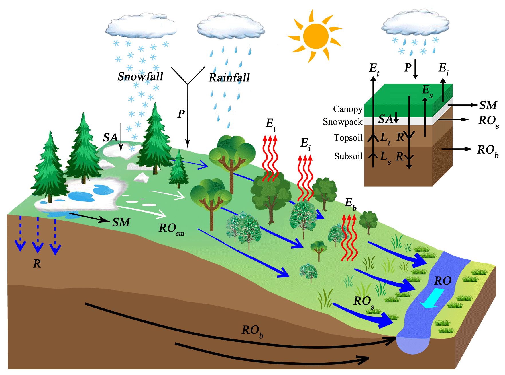
Figure 2Schematic diagram of the relative physical processes included in the construction of the SZIsnow. The upper right subplot shows the variables used in the SZIsnow calculations at the pixel level. Full names of all the abbreviations in this figure are listed in Table S2.
2.3 Evidence of different drought types for the SZIsnow evaluation
We evaluated the ability of the SZIsnow and SZI to capture different types of droughts based on drought evidence. First, meteorological, hydrological, and agricultural drought evidence was identified based on precipitation, streamflow, and soil water storage, respectively, from the dataset of Pan et al. (2012) (as mentioned in Sect. 2.2) over 32 large basins. Then, the evidence was compared with the SZIsnow and SZI, calculated based on the GLDAS-2 product. In addition, for the convenience of comparison, we adopted the log-logistic distribution to standardize precipitation, streamflow, and soil water storage for the computation of the SPI (Mckee et al., 1993), standardized streamflow index (SSI; Vicente-Serrano et al., 2012), and standardized water storage index (SWSI; Aghakouchak, 2014).
We also selected the residual water–energy ratio (WER) as a comprehensive drought indicator to evaluate the SZIsnow. The WER is defined as the ratio of residual available water (P − ET) to residual energy (PET − ET) and can integrally reflect drought conditions by depicting variation in water–energy balance. The WER was first suggested by Liu et al. (2017) as many studies found that the ratio of sensible heat (the residual energy supply after dissipating through latent heat) to net radiation (total energy supply) is always raised under drought. Meanwhile, the ratio of residual available water to precipitation (total water supply) is always lowered under drought. Consequently, the WER is lowered during drought and can be used as a comprehensive drought indicator. Again, we used independent datasets (i.e., the CRU TS and GLEAM datasets) to globally calculate the WER and compare it with the SZIsnow and SZI. As for the SSI and SWSI, the WER was standardized for the calculation of the SWI.
3.1 Derivation of the SZIsnow
3.1.1 Physical representation of the SZIsnow and its derivation
The physical processes included in the construction of the SZIsnow are shown in Fig. 2. Six water budget components are involved in the procedure of hydrological accounting to determine the water demand over a region. The related variables comprise ET, PET, runoff, potential runoff, soil infiltration, potential soil infiltration, soil moisture loss, potential soil moisture loss, snow water equivalent (SWE) accumulation, potential SWE accumulation, snowmelt, and potential snowmelt. The monthly values of these variables were derived from land surface models, for instance, the GLDAS-2 Noah LSM in the present study. The prominent improvement of the SZIsnow is that it accounts for the influence of snowfall on hydrological processes (Zhang et al., 2019, 2015).
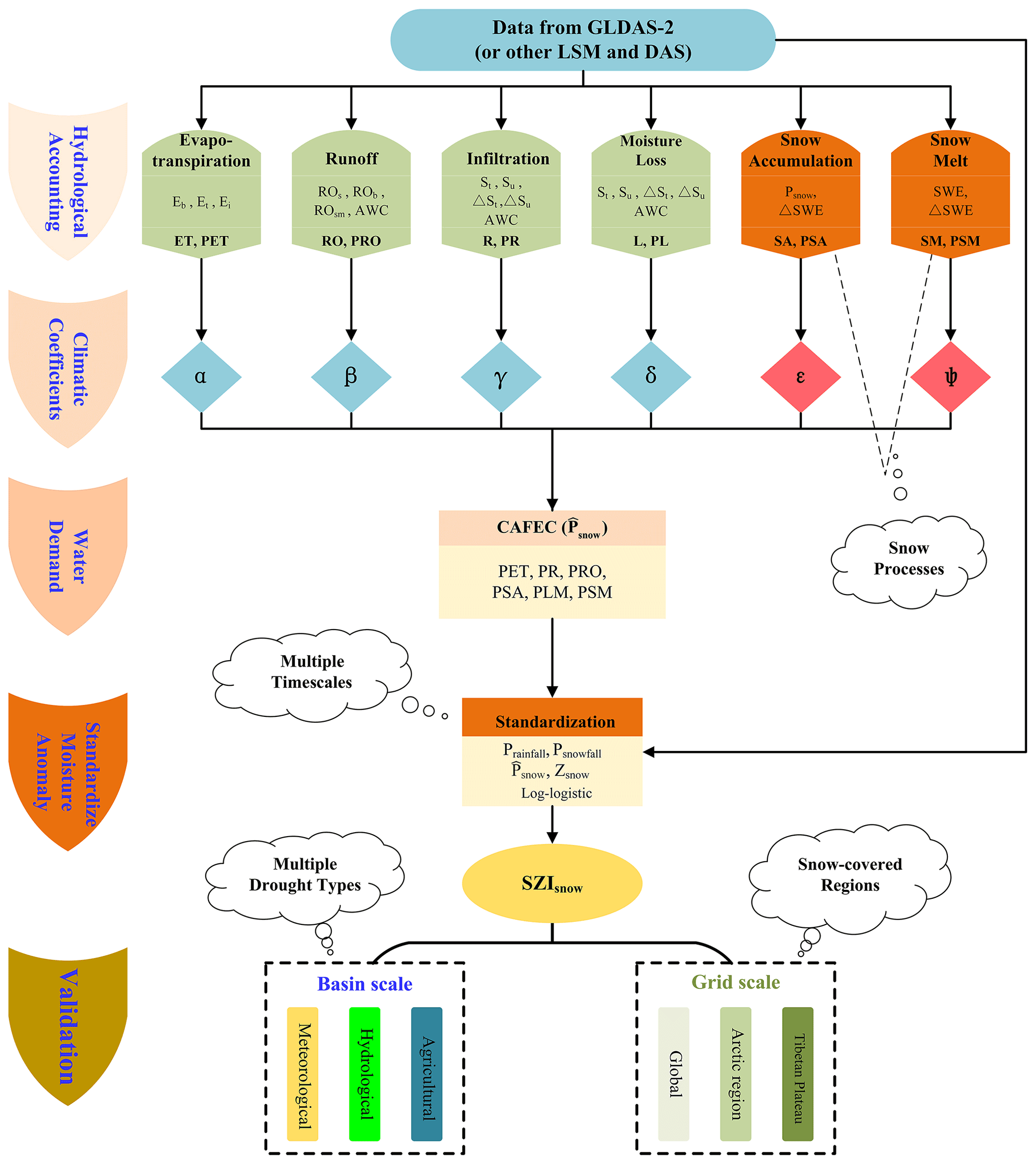
Figure 3The procedure flowchart describing the production and validation of SZIsnow. Variables derive the SZIsnow from GLDAS-2 (or other LSM and DAS). The production of SZIsnow includes four steps. The SZIsnow is validated at basin scale for three types of drought and at grid scale across different regions worldwide. The cloud-shape annotation shows the advantages of the SZIsnow.
Both the soil moisture storage and snow storage are considered reservoirs in the SZIsnow. Changes in soil moisture storage (soil infiltration or soil moisture loss) and snow (SWE accumulation or snowmelt) can alter the regional water balance (water supply or water demand) and then affect the drought condition. Consequently, the SZIsnow contains more comprehensive hydrological processes than the SZI. The improvement of the SZIsnow makes it applicable to a wider variety of climatic regions, especially for regions that belong to the three poles where more snow is stored than at any other place on Earth.
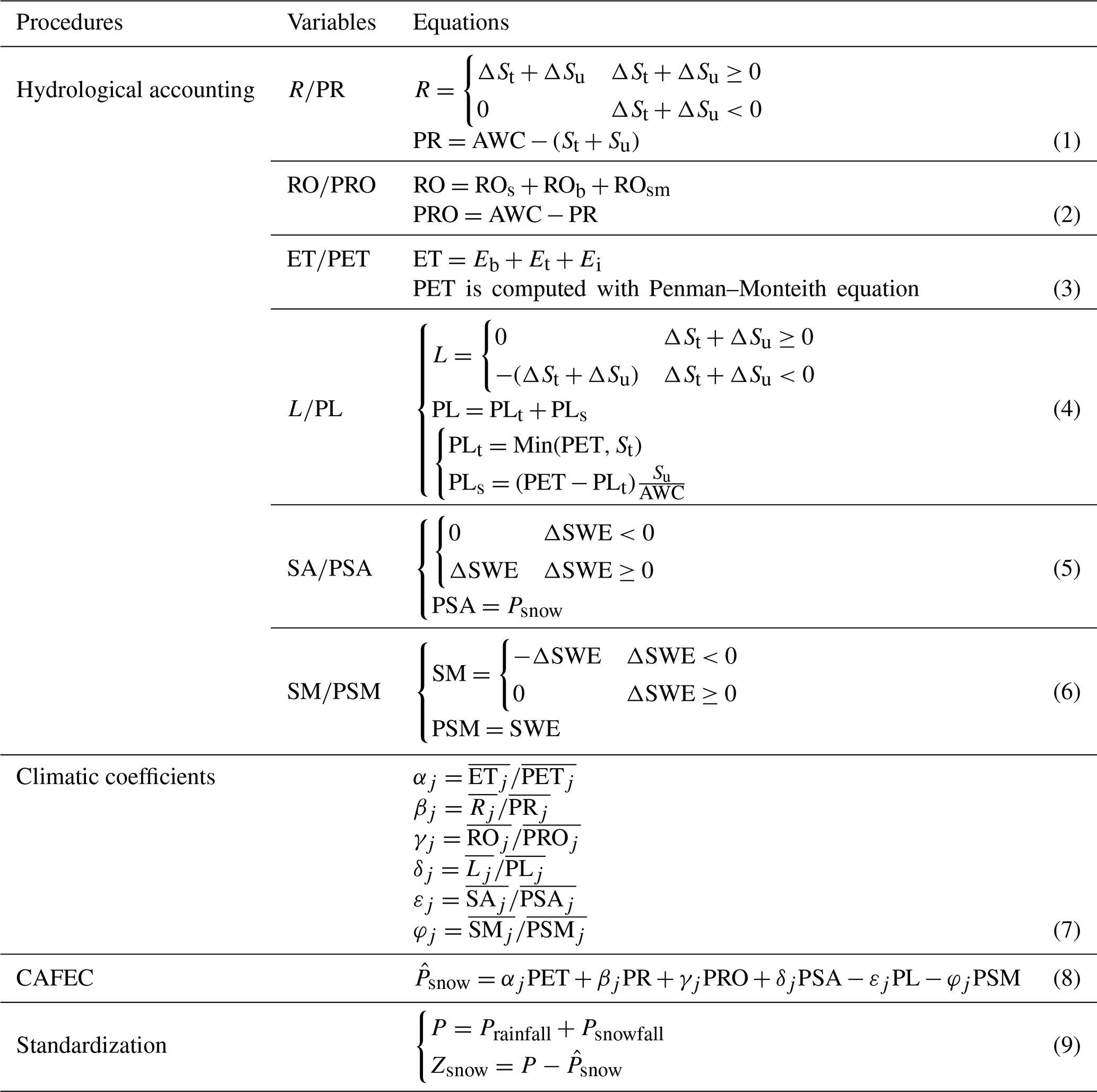
Table 1The procedures, variables, and associated equations used to calculate the SZIsnow.
We provide a procedure flowchart as shown in Fig. 3 to show the production and validation of the SZIsnow. There are four steps for SZIsnow production: hydrologic accounting, climatic coefficients, water demand, and standardization. Hydrologic accounting is to calculate the monthly six components relevant to the local water budget. Climatic coefficients are the weighting factors of these components for the calculation of the local water demand. The local water demand in the SZIsnow is represented by the precipitation that is climatically appropriate for existing conditions (CAFEC, referred as ). The last step is the standardization of the moisture anomaly (Zsnow), which is the difference between the actual precipitation (rainfall and snowfall). After achieving the SZIsnow dataset, its ability to identify different types of drought can be validated not only at basin scale, but also across different regions worldwide, especially snow-covered regions, at grid scale. Detailed equations for the hydrologic accounting in the SZIsnow are listed in Table 1. All full names for abbreviations contained in the equations are supplied in Table S2 in the Supplement.
3.1.2 Hydrologic accounting
The regional water supply firstly meets water demand from soil layers. The soil infiltration (R) was estimated by monthly changes (ΔSt and ΔSu) in available soil moisture of the top (St) and bottom (Su) soil layers. The potential soil infiltration (PR) was calculated as the difference between the available soil water capacity (AWC) and the available soil moisture of the entire soil. AWC is estimated as the maximum soil water of the two soil layers (Fig. 2) in the Noah LSM. Then, the rest of the regional water supply satisfies water demand from runoff (RO). RO consists of surface runoff (ROs), baseflow (ROb), and snowmelt runoff (ROsm), which are directly obtained from the GLDAS-2. The potential runoff (PRO) is the difference between AWC and PR, because soil moisture storage is considered a water reservoir in the SZIsnow. Additionally, water supply is partly consumed by ET, including bare soil evaporation (Eb), transpiration (Et), and canopy water evaporation (Ei) that can be found in the output of GLDAS-2. The PET is computed with output fields from GLDAS-2 using the Penman–Monteith equation. Moreover, the moisture loss (L) from the soil layers is considered in the SZIsnow. The equations for L and its potential values are shown in Eq. (4) of Table 1. Lastly, calculations of variables related to snow processes underscored by the SZIsnow are given in Eqs. (5) and (6) of Table 1. The potential snow accumulation (PSA) equals the monthly amount of snowfall (Psnow), and the monthly SWE change completely reflects snow accumulation (SA) and snowmelt (SM).
3.1.3 Climatic coefficients and precipitation that are climatically appropriate for existing conditions (CAFEC)
Similar to the PDSI, the SZIsnow applies the CAFEC () to quantify the regional water demand. The amount of is the result of interaction among the six water budget components as shown in Eq. (8) of Table 1. The weighting factor for each component is the climatic coefficient, which is defined as the ratio of the monthly climatic averages of actual (water supply) to potential (water demand) values. The equations used to compute these climatic coefficients are listed in Eq. (7) of Table 1. The j in Eq. (7) denotes months of a year; that is, each water budget component has 12 values of climatic coefficient covering all months. In addition, our equations can be applied in regions and seasons without snowfall. For regions without snowfall (e.g., tropics), the items relevant to snow in the equations of Table 1 are set to zero for the calculation of SZIsnow. For example, δjPSA, φjPSM, and Psnowfall are set to zero when they are used for situations without snowfall.
3.2 Standardization of moisture anomaly
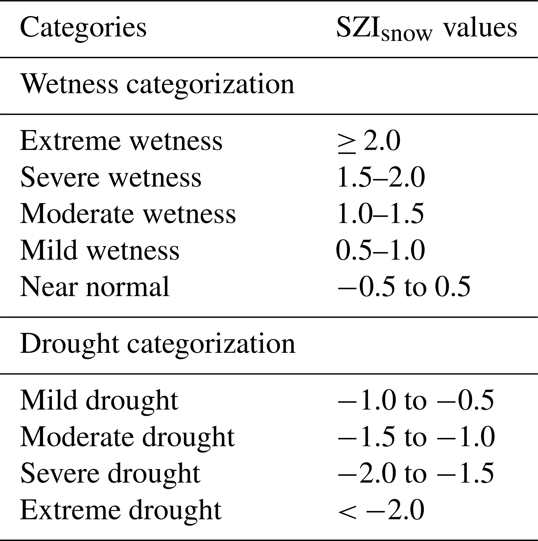
The comparison between the actual precipitation (P) and can reflect the drought condition. When the actual P is less than , the regional water supply will remain in deficit, and vice versa for a surplus. Thus, the difference between the actual P and is an appropriate indicator for regional water deficiency or surplus. Such difference is defined as the moisture anomaly Zsnow (Eq. 9 of Table 1) in the drought assessment system of the SZIsnow. In addition, the Zsnow can be aggregated at different temporal scales (e.g., 1–48 months) with the same processes as for the SPEI. For a detailed procedure, readers should refer to the paper of Vicente-Serrano et al. (2010). Moreover, we standardized the Zsnow to SZIsnow to realize the comparability of the Zsnow with other Zsnow or other drought indices over space and time. A three-parameter log-logistic distribution was adopted to standardize Zsnow time series and derive the SZIsnow. This follows the same approach used for the SPEI and SWI to standardize Zsnow at different temporal scales. The average value of the SZIsnow is 0, and the standard deviation is 1. Finally, we scaled the SZIsnow categorization levels to the corresponding SPEI drought severity categories in Table 2 because the same standardization method is used for both.
Table 2Categorization of wetness and drought conditions in the SZIsnow.
3.3 Metrics for the SZIsnow evaluation
This study applied the SPI (a meteorological drought index), SSI (a hydrological drought index), SWSI (an agricultural drought index), and SWI (a comprehensive drought index) as references to evaluate the performance of the SZIsnow and SZI. The four referenced drought indices were computed with datasets that were independent from the dataset used for calculating the SZIsnow and SZI. We utilized Pearson correlation coefficients (r) of SPI-SZI SZIsnow, SSI-SZI SZIsnow, SWSI-SZI SZIsnow, and SWI-SZI SZIsnow to compare the performance of the SZI and SZIsnow in terms of their capacity to capture multitype and multiscalar drought across different geographical parts of the world.
3.4 Identification of large-scale drought events in space and time
Using the SZIsnow dataset constructed by this study, we performed a global and continental drought analysis for the period 1948–2010. We focused on the temporal variability of large-scale drought events through a severity–area–duration (SAD) drought diagnosis method (Andreadis et al., 2005; Herrera-Estrada et al., 2017). In contrast to traditional studies which analyze the intensity, severity, and duration of drought over a fixed region, the SAD method specializes in simultaneously tracking the development of droughts in space and time based on a gridded dataset. This method proposes a Lagrangian approach by aggregating grids (under specified drought levels) of contiguous areas into clusters. These clusters are then tracked and archived as they propagate through space and time. The main steps of the SAD method are outlined as follows.
The SAD method firstly uses a monthly three-dimensional (3D, month × latitude × longitude) gridded drought index dataset to identify two-dimensional (2D, latitude × longitude) drought clusters in each time step. This drought cluster identification procedure is built on a clustering algorithm that merges spatial contiguity. Then, a median filter is utilized to smooth out noise (i.e., small-scale heterogeneity) in the 2D clusters in each time step. Specifically, we regarded a grid with a SZIsnow value below −1.0 as being under drought and considered connected areas within which all the grids had a SZIsnow below −1.0 as a drought cluster. The last step of the clustering procedure is to remove clusters with an area less than 500 000 km2. The remaining clusters are regarded as separate drought events for each time step. Additionally, droughts in the Sahara were not concerned in our study. During the SAD analysis, clusters were allowed to propagate into the Sahara (20–25∘ N, 17∘ W–34∘ E), and these clusters would be retained if their centroids fell outside the Sahara. In contrast, drought clusters were discarded if their centroids locate in the Sahara. More importantly, these identified drought clusters are allowed to split or merge through time in the SAD method. The tracking algorithm links clusters that have overlapping grid cells and records the merging or splitting date, areas, and centroids of clusters. These functions in the SAD method make it possible for us to monitor the spatiotemporal evolution of large-scale drought events. A large-scale drought event in North America identified by the SAD method is given as an example in Fig. S2 in the Supplement to illustrate this method.
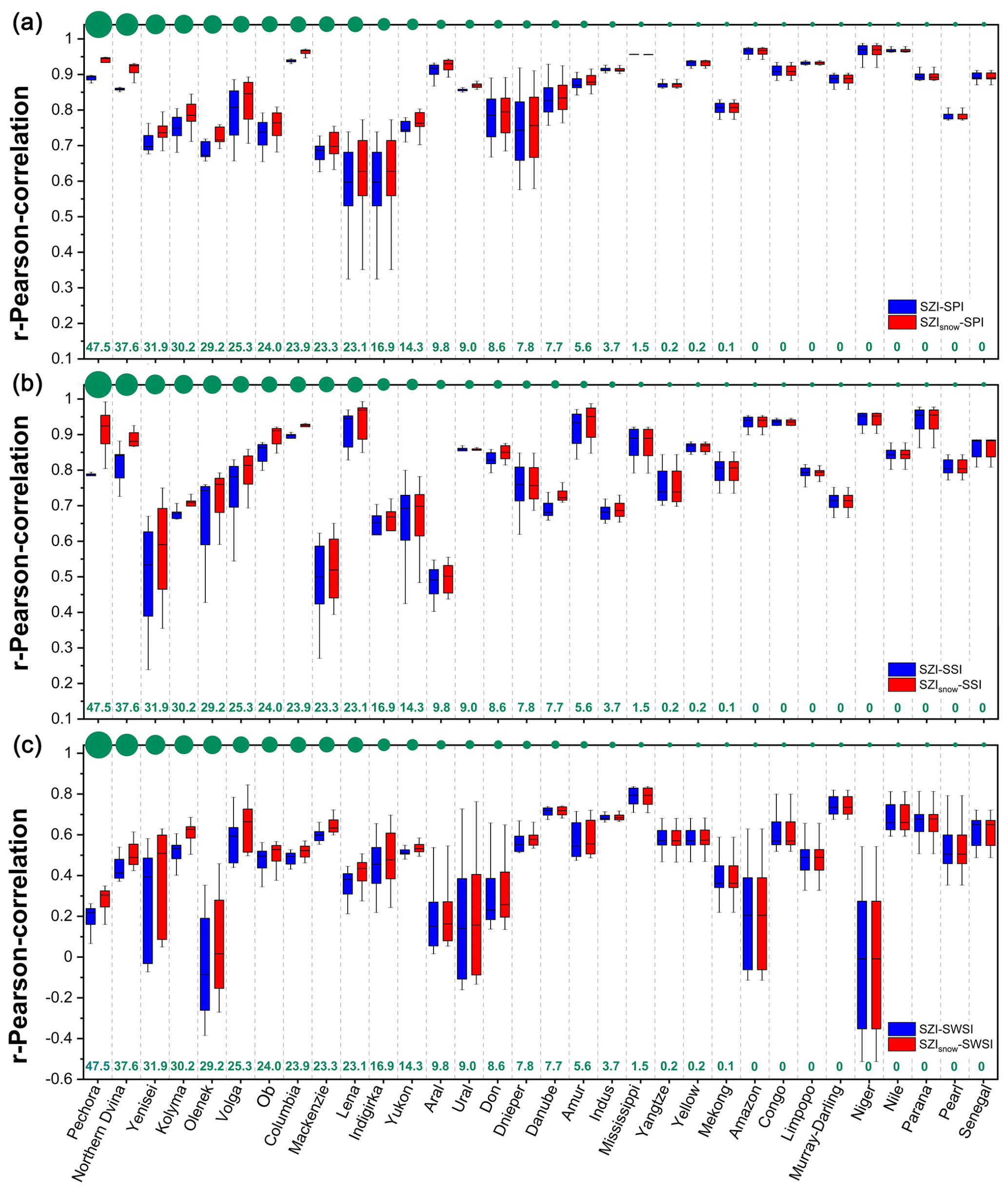
Figure 4Comparisons between the SZIsnow and SZI with regard to their performance in quantifying different types of drought. The SZIsnow and SZI were correlated with observed drought indices across the 32 basins. The Pearson correlation coefficient (r) was applied to evaluate the correlation. (a) Performance of the SZIsnow in quantifying meteorological drought. The blue boxes represent the statistical distribution of r between the SZI and SPI for timescales from 1 to 48 months in each basin, while the red boxes represent that between the SZIsnow and SPI. (b) Performance of the SZIsnow in quantifying hydrological drought (boxes represent same parameters as in (a) but correlations are with the SSI instead of the SPI). (c) Performance of the SZIsnow in quantifying agricultural drought (boxes represent same parameters as in (a) but correlations are with the SWSI instead of the SPI). Basins were ranked in descending order based on their SWE. The green dots along the top of each x axis denote the SWE of each basin, and their sizes were scaled by the green SWE values given along the bottom of each x axis.
4.1 Evaluation of the SZIsnow
4.1.1 Evaluation of the SZIsnow for different drought types
We firstly evaluated the capability of the SZIsnow to capture meteorological drought at different temporal scales over the 32 large basins from 1948 to 2010 and compared this to the capability of the SZI. The observation-based meteorological drought index, SPI, was used as a reference. As shown in Fig. 4a, the blue boxes represent the statistical distribution of the Pearson correlation coefficient (r) between the SZI and SPI for 1–48-month timescales in each basin, while the red boxes represent that between the SZIsnow and SPI. The SZIsnow generally outperformed the SZI over these large basins with an average improvement of 3.19 % (ranging from 0.01 % to 6.45 %). It is clear that the extent of improvement in the SZIsnow increases as the SWE increases. For instance, the r of the SZIsnow–SPI is 5.51 % higher than that of the SZI–SPI in the Pechora basin that has an SWE of 47.5 mm yr−1. In contrast, the r of the SZIsnow–SPI is only 0.11 % higher than that of the SZI–SPI in the Indus basin that has an SWE of 3.70 mm yr−1. The relationship between the enhancement in the SZIsnow and SWE implies that the SZIsnow brings advantages in accounting for snow processes. It also demonstrates that the SZIsnow appropriately reflects the fact that snow accumulation and melt have considerable impacts on the seasonal and inter-annual variation in streamflow in snow-covered areas. In addition to the SPI, we adopted two other mainstream drought indices (SPEI and scPDSI) to compare their performance in monitoring meteorological drought. As shown in Fig. S3 in the Supplement, the performance of SZIsnow is prominent and superior to SZI, SPEI, and scPDSI in identifying meteorological drought at multiple temporal scales. The selection of reference drought indices did not influence the reliability of our conclusion. In summary, the SZIsnow has a satisfactory performance to capture meteorological drought.
We then evaluated the capability of the SZIsnow to capture hydrological drought (Fig. 4b). The observation-based hydrological drought index, SSI, was used as a reference. The SZIsnow generally outperformed the SZI over these large basins, with an average improvement of 3.13 % (ranging from 0.25 % to 17.53 %). The extent of improvement in the SZIsnow increases as the SWE increases. For instance, the r of the SZIsnow–SSI is 17.53 % higher than that of the SZI–SSI in the Pechora basin that has an SWE of 47.5 mm yr−1. In contrast, the r of the SZIsnow–SSI is only 1.18 % higher than that of the SZI–SSI in the Indus basin that has an SWE of 3.70 mm yr−1. Moreover, among the multiple temporal scales over which it was tested, the SZIsnow performs best at the 12-month scale for hydrological droughts. At the 12-month scale, the SZIsnow performs 17.53 %, 11.46 %, 19.40 %, and 4.88 % better than the SZI in the Pechora, Northern Dvina, Yenisei, and Kolyma basins, respectively. Thus, the SZIsnow performs well in the context of capturing hydrological drought.
The capability of the SZIsnow and SZI to capture agricultural drought was also assessed in our study. We conducted the same steps of assessment as those for assessing hydrological drought, but the reference drought index was an agricultural drought index, SWSI, derived from a dataset based on observations. As shown in Fig. 4c, the average r of the SZIsnow-SWSI for all the basins is 0.51 (ranging from 0.19 to 0.79), which indicates the ability of the SZIsnow to reliably capture agricultural drought. Additionally, the SZIsnow performs better than the SZI in almost all basins, and the average improvement of the SZIsnow is 6.46 % (ranging from 0.14 % to 38.96 %). Again, larger improvements occurred in basins with a larger SWE. This comparison, in terms of agricultural drought, again emphasizes the strength of the SZIsnow in high-latitude and high-altitude regions with relatively greater SWE. The SZIsnow thus performs sufficiently well to capture agriculture drought. Besides the outperformance of the SZIsnow, it should be noted that the SZIsnow has a similar performance with SZI over the snow-free basins. Such similar performance is mainly owing to the fact that the values of Psnow, PSM, and PSA are close to zero over basins at low-latitude and low-altitude (snow-free) areas, leading to the calculation of SZIsnow converging to the snow-free basins. Therefore, the performance of SZIsnow and SZI is consistent over snow-free areas.

Figure 5Performance of the SZIsnow over different latitudes (a, b) and specifically over the Arctic region (c, d). Here the differences between the correlation coefficients of the SZIsnow–SWI and those of the SZI–SWI for different timescales were used to compare their performance. (a) The Hovmöller diagram (timescale × latitude) shows the differences averaged by latitude from 55∘ S to 85∘ N for timescales ranging from 1 to 48 months. (b) Distribution of the difference for specific timescales (6, 9, 12, and 15 months) with changing latitude. (c) Spatial distribution of the differences between the correlation coefficients of the SZIsnow–SWI and those of the SZI–SWI over a 12-month timescale in the Arctic region. (d) Variations in correlation coefficients averaged over the Arctic region for various temporal scales. The shading denotes the range of correlation coefficients. The upper (lower) boundary is the maximum (minimum) value. The inset shows the change of relative difference (%) for these temporal scales.
4.1.2 Evaluation of the SZIsnow across different spatial scales
The SZIsnow can be computed and used to characterize drought for an individual grid, although we evaluated its capability at a basin scale in Sect. 4.1.1. In this section we apply the SWI drought index as a reference to assess the SZIsnow at the global scale (Fig. 5a and b). The Hovmöller diagram (Fig. 5a) shows the distribution of the difference between the r of the SZIsnow–SWI and that of the SZI–SWI for 1–48-month timescales across different latitudes. It is clear that the high-value zonal mean difference mainly centers in the interval of 50–65∘ N. This indicates that the SZIsnow outperformed the SZI within this 15∘ interval in high-latitude areas. In contrast, the remaining regions, outside of this interval, show only small magnitude differences. In addition, as shown in Fig. 5b, the improvement of the SZIsnow varies over different timescales; it performs better over timescales in the range of 3–12 months. Such spatial patterns, as shown in Fig. 5a and b, emphasize the physical improvement in terms of snow processes in the SZIsnow construction compared to the SZI. This evaluation shows the appropriate performance of the SZIsnow at the global scale.
As the three-pole region is a focus of this study, we specifically compared the SZIsnow and SZI over the Arctic region, where the latitude is larger than 66∘33′ N. Figure S4a and b in the Supplement present the spatial distributions of the r of the SZIsnow–SWI and SZI–SWI, respectively, over a 12-month timescale. The two maps show similar spatial patterns for the SZIsnow and SZI, yet the r of the SZIsnow–SWI is larger than that of the SZI–SWI over the majority of the Arctic region, indicated by the positive difference shown in Fig. 5c. Once again, the SZIsnow is seen to outperform the SZI over the Arctic region, which is consistent with the findings from the global evaluation shown in Fig. 5a and b. Additionally, the relationship of area-averaged r and timescales is shown in Fig. 5d. The maximum r appears when the timescale is 12 months, and the relative difference between the r of the SZIsnow–SWI and that of the SZI-SW (i.e., the improvement of the SZIsnow) shows a rapid growth moving from 1- to 12-month timescales (Fig. 5d, insert plot). The results demonstrate that the SZIsnow dataset performs well over the Arctic region.
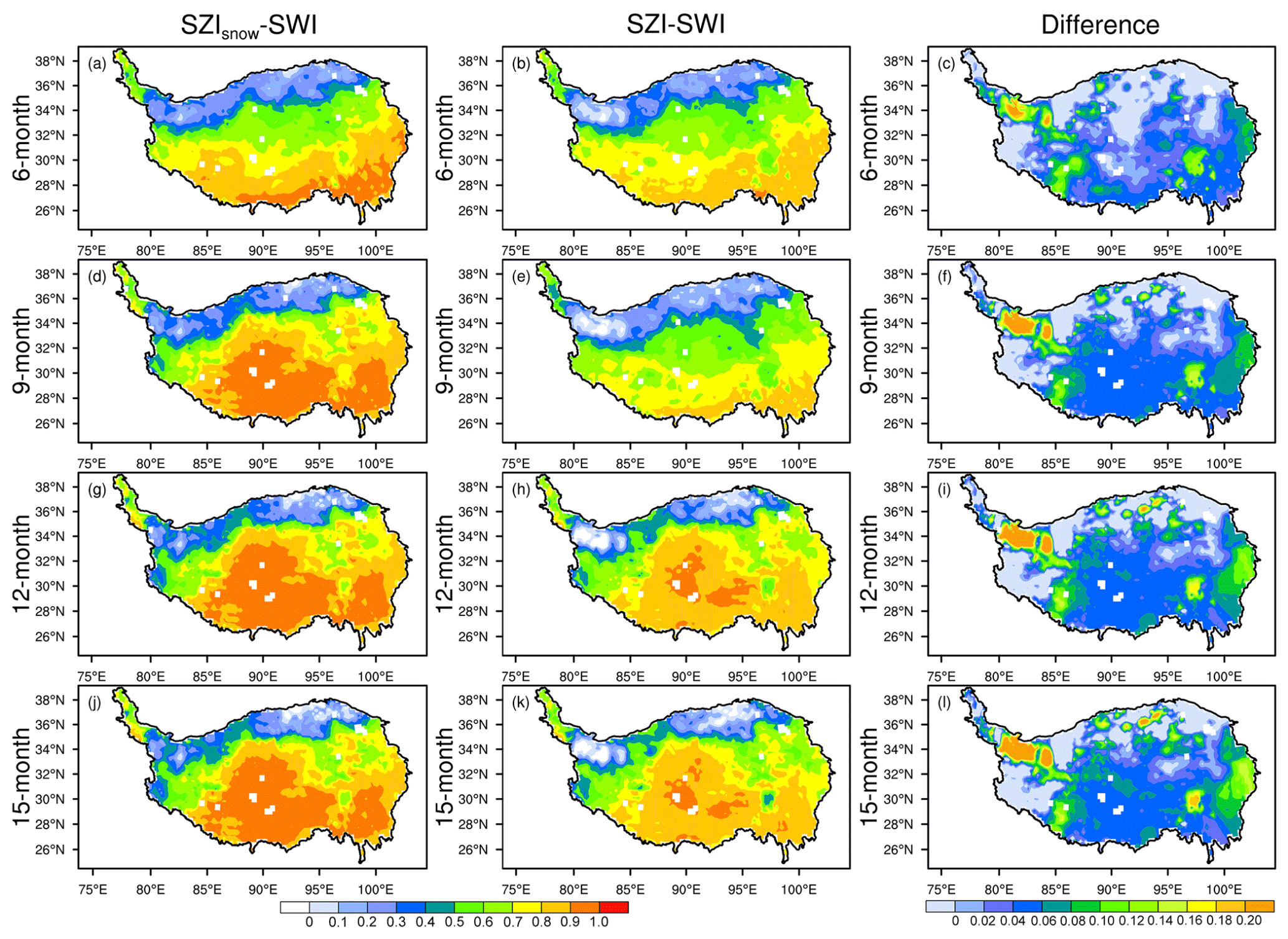
Figure 6Spatial distribution of correlation coefficients of the SZIsnow–SWI (left column, a, d, g, j) and those of the SZI–SWI (middle column, b, e, h, k), and the differences between the two (right column, c, f, i, l show the left column minus middle column) over the Tibetan Plateau at different timescales (6, 9, 12, and 15 months).
The risk of drought on the Tibetan Plateau, the world's third pole, can affect the water supplies of billions of people. Figure 6 shows the capability of the SZIsnow and SZI to capture drought at various temporal scales over the Tibetan Plateau. Both the SZIsnow and SZI have high r values with the SWI over a large part of the Tibetan Plateau. The r of the SZIsnow–SWI is larger than 0.6 across 68.96 % of the entire Tibetan Plateau, and for the SZI–SWI this value is 61.93 % (Fig. 6, left and central columns). The area-averaged r of the SZIsnow–SWI is 0.72, and that of the SZI–SWI is 0.65 over a 12-month timescale, equating to an improvement of 10.77 % for the SZIsnow. Moreover, the phenomenon that the SZIsnow outperforms the SZI is clearly shown in the right column of Fig. 6. The largest improvement is seen mainly in the northwest corner and southeastern part of the Tibetan Plateau, where the largest snow depths are also seen (Dai et al., 2017). Thus, the SZIsnow dataset is a reliable resource to quantify drought across the Tibetan Plateau.
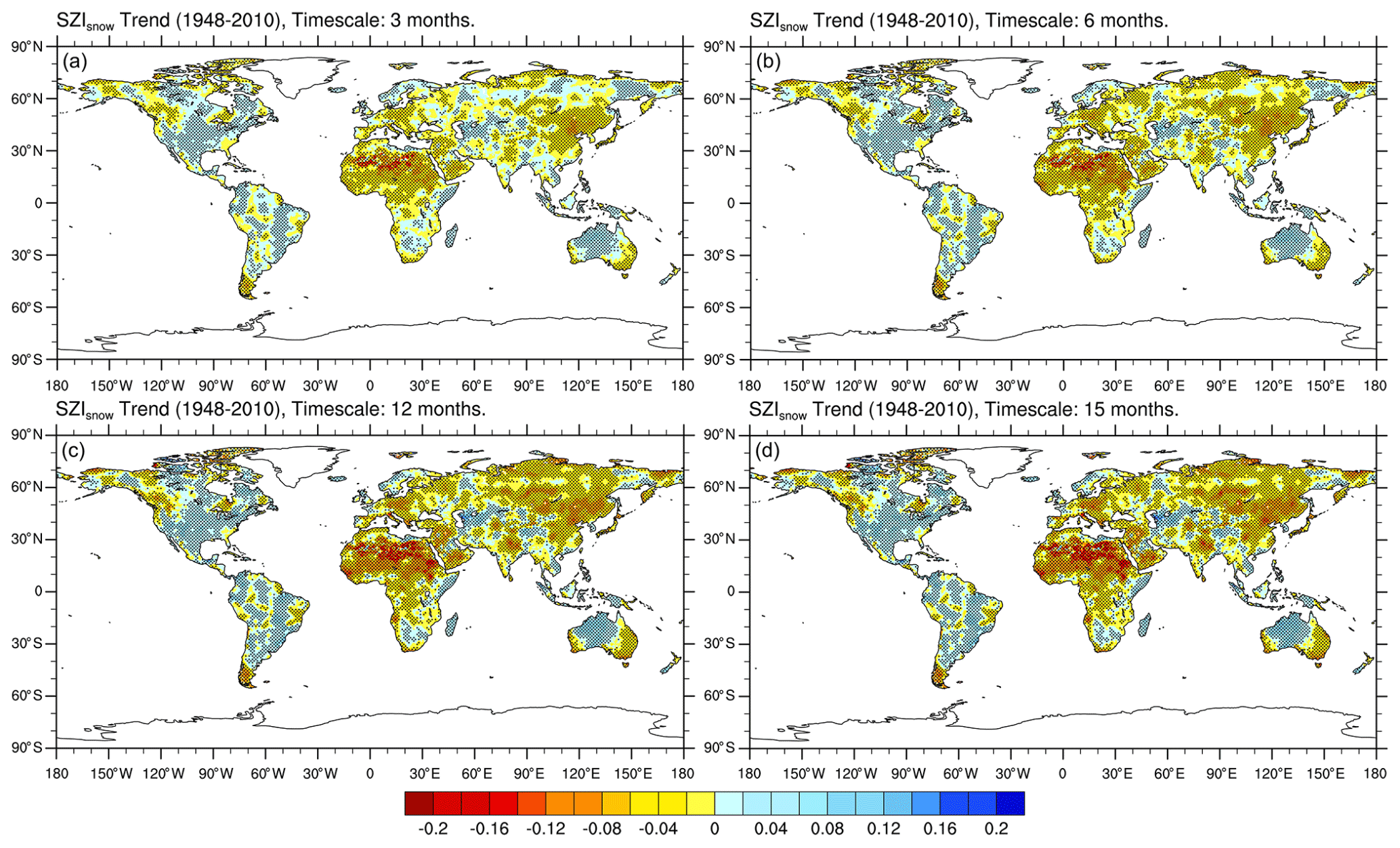
Figure 7Spatial distribution of the linear annual trend (changes per 50 years) in the SZIsnow during the period 1948–2010, at various timescales. The stippling denotes the trend being statistically significant at the 95 % confidence level.
4.2 Historical trends in global drought
The proposed SZIsnow dataset was applied to investigate the historical changes in global drought between 1948 and 2010. The spatial distribution of the linear annual trend in the SZIsnow over different timescales (i.e., 3, 6, 12, 15 months) is shown in Fig. 7. The SZIsnow at each temporal scale demonstrates a similar global pattern, except for differences in the magnitude of dryness or wetness trends. Overall, 59.66 % of the land area of the Earth displays a drying trend, and the remaining 40.34 % exhibits a wetting trend. As shown in Fig. 7, the SZIsnow shows a drying trend over eastern Asia, northern India, most of the Arabian Peninsula and Africa, eastern Australia, and central and southern Europe; increased wetness was found over most of the United States, a large part of South America, and central Australia. Our study excluded Greenland due to its sizable ice-capped area, about 80 % of the island. Additionally, the drying trend tends to increase as the timescale becomes longer. For instance, the drying rate of the SZIsnow over eastern Asia becomes larger as its timescale increases. Moreover, our results are broadly consistent with the findings of Dai (2013), who analyzed the trend of global drought using the self-calibrated PDSI. This also implies that the SZIsnow is a useful proxy of aridity changes.
We further examined variations in the area of global land under drought (Fig. 8a). The area under drought shows an increasing trend with an average rate of increase of 0.05 % yr−1. Large fluctuations began to emerge from 1975, and Earth's drought area increased rapidly in the early 1980s. This growth was largely attributed to the leap in temperature caused by the 1982–1983 El Niño (Timmermann et al., 1999; Dai, 2011b). The maximum extent of drought area appeared in 1991. Moreover, the temporal change in the global moisture anomaly Zsnow is shown in Fig. 8b. The Zsnow displays a global downward trend of −0.11 mm yr−1 for the period 1948–2010, which indicates the increasing global deficit between water supply and water demand. Overall, our analysis based on the SZIsnow dataset revealed increased aridity over many land areas and severe and widespread droughts over the Earth since 1948.
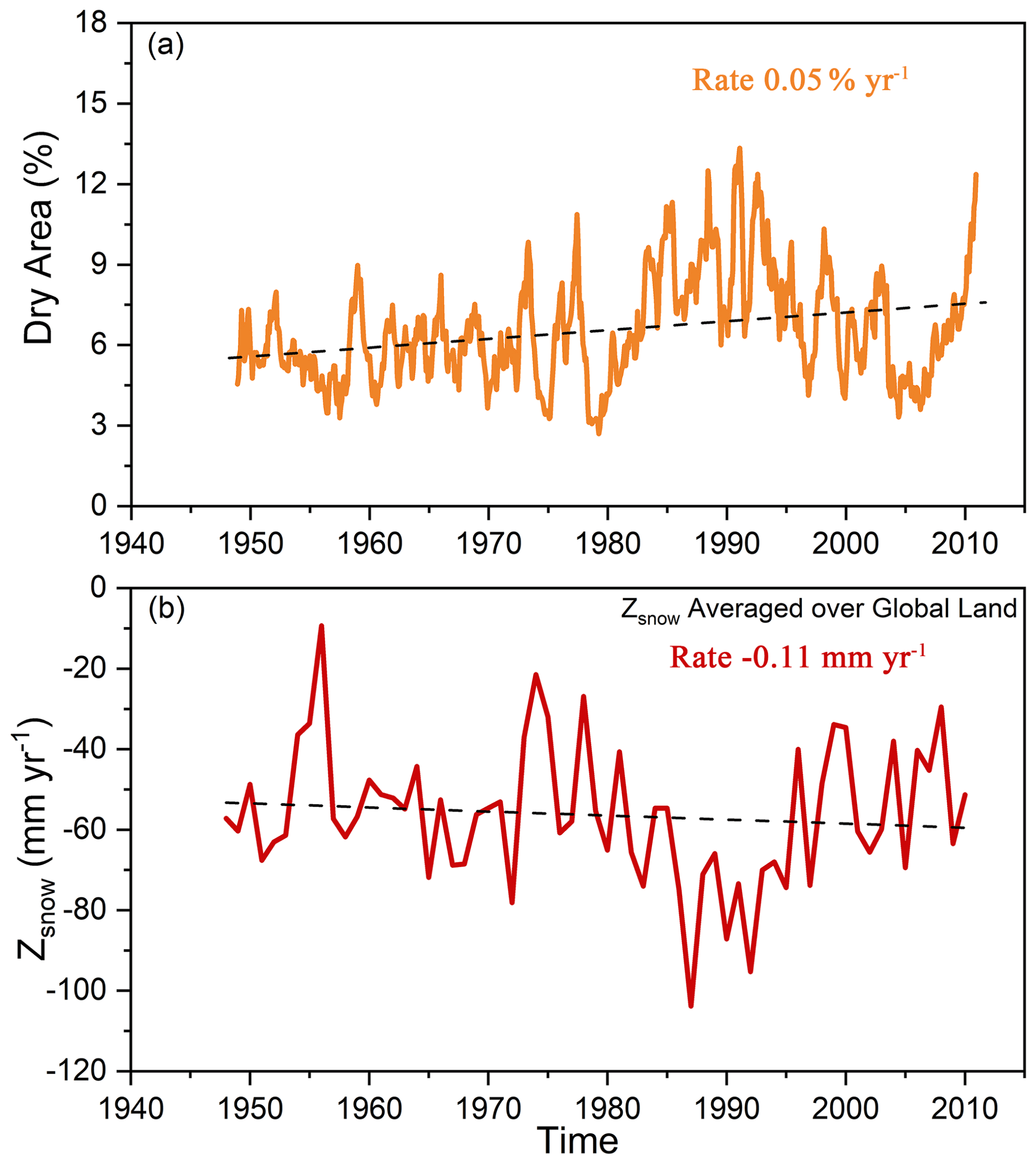
Figure 8Time series of (a) global dry land area (% yr−1) and (b) Zsnow (mm yr−1) between 1948 and 2010. The dry land area was calculated based on the SZIsnow at a 12-month timescale. The dashed lines denote the linear trends.
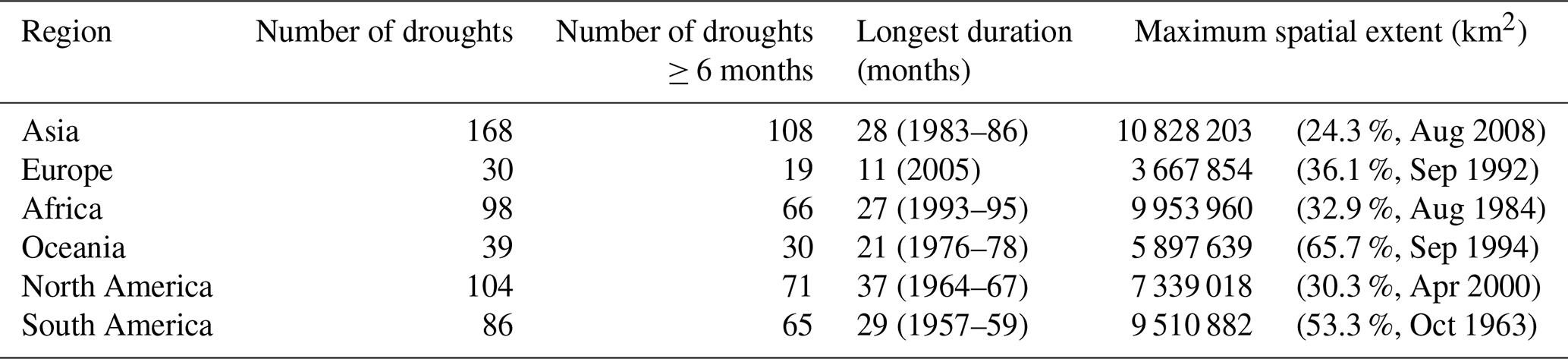
Table 3Summary of large-scale drought occurrence for each continent. In the fourth column, the duration of the drought is shown in months, and the period is listed in parentheses. In the final column, the spatial extent is given as a percentage of the total continental area, and the date at which the maximum spatial extent occurred is listed in parentheses.
4.3 Global and continental large-scale drought events
4.3.1 Statistics of large-scale drought events
Using the SZIsnow dataset proposed in this study, we analyzed global and continental large-scale drought events (hereinafter referred to as drought) from 1948 to 2010 by leveraging the SAD drought diagnosis method. There have been 525 droughts with an area larger than 500 000 km2 globally during the study period, as shown in Table 3. Also outlined in Table 3 is detailed information for the droughts with the longest duration and the largest area, respectively, for each continent. Droughts with a duration longer than 6 months account for nearly 70 % of all droughts. The longest drought that occurred in North America lasted 37 months from 1964 to 1967. The most spatially extensive drought occurred over Asia in August 2008 (drought lasted from November 2007 to June 2009) and covered an area of approximately 11×106 km2 (roughly 100 times Guatemala's national territory area of 108 889 km2). For comparison, the most extensive drought in Oceania covered nearly 66 % of its continental area (roughly 54 times the size of Guatemala). Here Oceania is defined as Australia, New Zealand, Papua New Guinea, and the Pacific Islands.
We further ranked the top five droughts in terms of duration and maximum spatial extent for each continent (Table 4). For Asia, the longest drought lasted 28 months, and its droughts commonly extend across larger areas compared to other continents. The top five longest droughts in Europe had a relatively short duration compared to other continents. In Africa, the longest drought lasted 27 months, and the maximum extent was 10×106 km2. Of all analyzed droughts, 60 % occurred in the period from the mid-1980s to the mid-1990s; it is clear that there was a prolonged drought spell over this period. Moreover, the droughts in North America always have a longer duration compared to other continents.
Table 4Top five drought events in each continent, ranked by duration, or by maximum spatial extent. The duration and spatial extent are listed in parentheses after the period of each drought event.

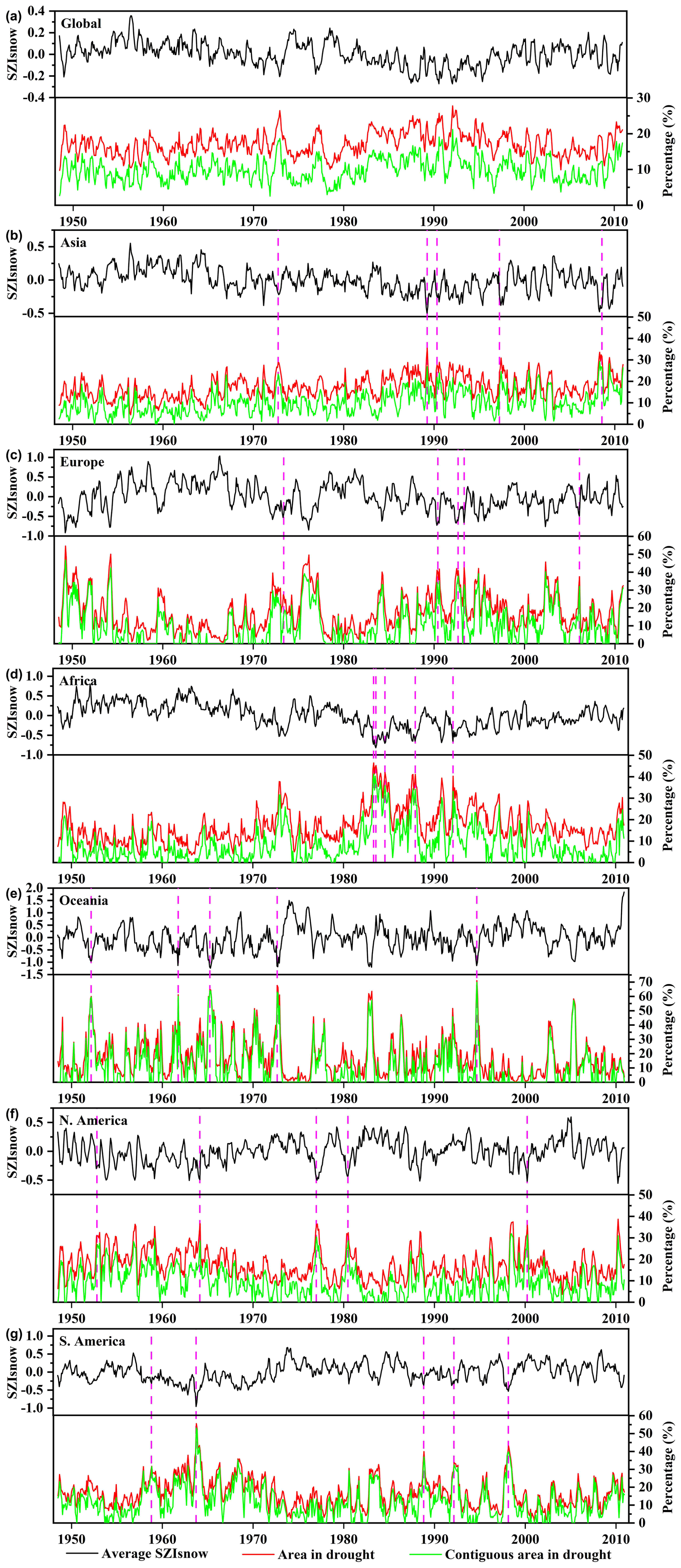
Figure 9Temporal variation in monthly area-averaged SZIsnow (black lines), the area in drought (pixels with SZIsnow < −1, red lines), and contiguous area in drought (green lines) for the world, Asia, Europe, Africa, Oceania, North America, and South America. The vertical pink dashed lines mark the top five major large-scale drought events in each continent.
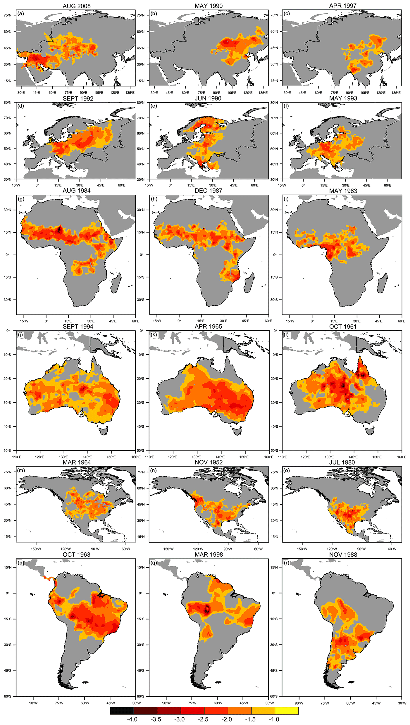
Figure 10Spatial distribution and severity of the major large-scale drought events for Asia, Europe, Africa, Oceania, North America, and South America. Three out of the top five drought events were selected here for each continent. The geographic coordinate system is used in this figure.
4.3.2 Temporal variability of large-scale drought events
The temporal variation in area-averaged SZIsnow, the area under drought (pixels with SZIsnow less than −1.0), and contiguous areas under drought are shown and analyzed in Fig. 9, in which the vertical pink dashed lines mark the top five most extensive droughts in each continent. We also selected three of the top five most extensive droughts to show their spatial distribution (Fig. 10). The global averaged SZIsnow displays a significant downward trend of −0.02 per decade (95 % confidence level, Fig. 9a), which indicates a global drying trend. This drying trend was closely related to increases in temperature over the study period. Accordingly, the global area under drought shows an upward trend (0.31 % per decade) and approaches a plateau over the period 1985–1995. It is clear that the contiguous area under drought demonstrates a similar pattern of variability to the area under drought for each continent and globally. Such similarity implies the large-scale drought identified by the SAD method can largely reflect the variability of the global area under drought.
Asia experienced a drying trend, based on the area-averaged SZIsnow, during the period 1948–2010 (Fig. 9b); the contiguous area under drought ranges from 0 % to 29.30 %, with an average of 10.14 %. With large fluctuation, droughts in early 1990s are salient features of the time series of Asia, and three of the five droughts with the largest spatial extent occurred during the 1990s. The drying trend in east Asia was mainly caused by weakening summer monsoons owing to changes in the El Niño–Southern Oscillation (ENSO) and the Pacific Decadal Oscillation (Zhang and Zhou, 2015). The large-scale severe droughts in the Middle East and southwest Asia were closely related to La Niña (Barlow et al., 2016). Additionally, the temporal variability within Asia is comparably small, mainly due to the dampening effect of its large spatial scale (Sheffield et al., 2009). In Europe, high variability of the contiguous area in drought was detected in the first half of the 1950s (Fig. 9c). The drought condition alleviated somewhat between the mid-1950s and the mid-1970s. The high variation was repeated in the 1990s and was associated with multiple periods of droughts with large spatial extent. In particular, large-scale droughts identified by the SZIsnow occurred with a greater frequency over central Europe compared to other parts of Europe. The leading driver behind this pattern was the significant increase in potential evapotranspiration (Spinoni et al., 2015a). The findings in Europe, based on SZIsnow, are broadly in agreement with other studies (Lloyd-Hughes and Saunders, 2002; Spinoni et al., 2015b).
In Africa, the area-averaged SZIsnow exhibits a visible drying trend from 1948 to 2010 (Fig. 9d). The time series of drought areas underwent a gradual climb and achieved a maximum value in the mid-1980s, with a severe drought period then lasting until the mid-1990s. All top five spatially extensive droughts are concentrated within this period and are commonly located to the south of the Sahara (Fig. 10g–i). Our results for Africa are generally similar to previous studies, which concluded that ENSO and sea surface temperature (SST) are the main driving forces of droughts across the entire continent (Masih et al., 2014). For Oceania, strong drought spells occurred frequently from the 1950s to the 1970s (Fig. 9e). This continent is characterized by its high percentage of large-scale drought areas, and multiple droughts account for more than 40 % of the total continent (Fig. 10j–l). The characteristics of historical droughts in Oceania are associated with variability of global climate, for instance, the Interdecadal Pacific Oscillation and Southern Annular Mode (Askarimarnani et al., 2021; Kiem et al., 2016).
In North America (Fig. 9f), the evident drought spells in the 1950s were captured by the SZIsnow, and the largest drought area covered 37 % of the entire continent. As shown in Fig. 10o, the drought in March 1964 covered most of the United States. Previous studies confirmed that the tropical part of the SST anomalies was primarily related to the most notable droughts of the 1950s in the United States (Schubert et al., 2004). Another two obvious drought signals are found in the late 1970s and 1990s. The droughts detected here with the SZIsnow show close correspondence to the findings of previous studies (Su et al., 2021; Andreadis et al., 2005). Moreover, notable distinct dry spells emerged in the 1960s and 1990s in South America (Fig. 9g). For instance, the largest drought in October 1963 covered up to 54 % of this continental area (Fig. 10r) and covered nearly the whole of Brazil. After a strong dry spell in 1998, South America exhibited a low percentage of drought extent until the end of the studied time series.
This study proposes a drought index dataset on the basis of a new drought index, SZIsnow, by incorporating snow dynamics into the SZI. Results from the evaluation of the SZIsnow dataset suggest that consideration of snow processes can improve the performance of the SZIsnow. The improvement is remarkable when the SZIsnow is applied in snow-covered areas, including high-latitude and high-altitude areas. Our results highlight the importance of snow in drought development because it can greatly affect the onset, cessation, severity, location, and duration of drought (Huning and Aghakouchak, 2020; Staudinger et al., 2014). Snow serves as the main water resource for many regions of the world (e.g., western United States) through its accumulation in the cold season and melting in the warm season. However, climate change is altering the effect of snow on the availability of water resources. Increasing temperature leads to less snowfall and earlier snowmelt and further results in a mismatch between the peak of streamflow and that of water demand, which can increase the drought risk over these regions (Adam et al., 2009; Özdoğan, 2011). The results of the present work underscore the importance of considering snow processes in drought quantification under global climate change.
Using the proposed SZIsnow dataset, this study emphatically analyzed the severity–area–duration of global and continental large-scale drought. The SZIsnow dataset achieved a satisfactory performance in monitoring the propagation of large-scale contiguous droughts through space and time. Using the SAD drought diagnosis method, the SZIsnow dataset appropriately captures the numbers and variability of historical large-scale contiguous droughts for each continent. These captured drought events are broadly aligned with findings from previous research (Zhang and Zhou, 2015; Mctainsh et al., 1989; Kiem et al., 2016; Lloyd-Hughes and Saunders, 2002). Such performance implies the present dataset can be applied globally to understand the mechanisms behind large-scale droughts. It also raises confidence in the ability of the SZIsnow to predict drought events, especially those with extensive spatiotemporal influence. Moreover, our results indicate that large-scale contiguous droughts control, to a large extent, the character of the variation in global drought. Thus, the capacity to track the evolution of large-scale droughts in space and time is a crucial aspect for the assessment of a drought index.
The SZIsnow absorbs the advantages of both the PDSI and SPEI and can be used to monitor multitype droughts at various temporal scales. Compared to the PDSI, it considers more hydrological components related to water supply and demand and quantifies their contribution to water demand by weight. Such consideration enhances the physical realism of drought quantification, particularly over high-latitude and high-altitude regions that usually receive substantial snowfall (Zhang et al., 2019). The enhancement achieved by the SZIsnow implies that more key physical processes should be considered when constructing a drought index, rather than using a simple generalization, although we admit that a sophisticated index is always limited by insufficient observation to some extent. However, data assimilation serves as a new way to overcome the difficulty of insufficient observation (Mishra and Singh, 2011). This new method combines a multi-source dataset and an advanced land surface model to provide optimal values of variables related to drought, which is the reason why we used GLDAS-2 as the forcing means of SZIsnow calculation. Therefore, the improvement of SZIsnow indicates that more attention should be paid to the combination of the drought index and the data assimilation system (DAS) or LSM.
The combination of the SZIsnow and the DAS provides the possibility to track droughts over ungauged areas. As more models (e.g., crop model, wildfire model, root model) have been coupled with the DAS, the combination between the SZIsnow and the DAS has become more physically realistic. Yet, uncertainties from the DAS will inevitably be introduced into the SZIsnow, which undermines the reliability of the SZIsnow. Previous studies have often obtained dissatisfactory results during the validation of GLDAS-2 (e.g., Fatolazadeh et al., 2020). These uncertainties originate from incomplete model structure, forcing data biases, and biases in parameter estimation (Qi et al., 2020). However, recent developments in LSMs, DAS techniques, and computational power are helpful in resolving issues associated with uncertainty. Thus, determining how to introduce uncertainty quantification when utilizing the SZIsnow to assess drought is a future goal of ours.
The SZIsnow is a comprehensive drought index because it incorporates different aspects of the hydrologic cycle, which provides a clear-cut way to synthesize different kinds of information related to drought into a simple message. Such synthesizing capacity is particularly crucial because droughts have a broadly adverse influence on agricultural water, municipal water, energy supply (hydropower), and human and animal safety. Thus, the SZIsnow has a high potential to be utilized for drought management. Currently, however, the SZIsnow is mostly used only by the scientific community (Lu et al., 2020; Ayantobo and Wei, 2019) and rarely used by decision- and policy-makers. One reason for this is that the acquisition of best-fit thresholds in the SZIsnow, for one type of drought over an area with a specific climate regime, requires a trial-and-error approach and takes time. On the other hand, drought management is a synergistic effort involving a variety of sectors and requires joint operations of these sectors. Additionally, the complexity of calculations is a limitation of the SZIsnow. Therefore, it is necessary to strengthen the user-friendliness of the SZIsnow and collaborate closely with government departments related to drought management.
All datasets used in this work are freely available. The SZIsnow dataset proposed by this work is a good contribution to the study of climate change, ecology, and hydrology. It is especially helpful for research focusing on spatiotemporal dynamics of drought, the underlying mechanisms of drought evolution, and the development of drought indices. The dataset contains 48 individual files with timescales of 1–48 months and has been archived in the Network Common Data Form (NetCDF) format. The monthly SZIsnow in each file covers the Earth's land area and has a spatial resolution of 0.25∘ from 1948 to 2010. The SZIsnow dataset is freely downloadable from the Zenodo repository at the following DOI: http://doi.org/10.5281/zenodo.5627369 (Wu et al., 2021). In addition, we also published the dataset to the National Tibetan Plateau/Third Pole Environment Data Center, which has been accredited by the Earth System Science Data and specializes in collecting, integrating, and publishing geoscientific data on and surrounding the Tibetan Plateau and the three poles (Li et al., 2020; Pan et al., 2021). The SZIsnow dataset can be downloaded from this data center at the following URL: http://data.tpdc.ac.cn/en/data/b039fde6-face-4d24-af45-d238a6af18b7/ (last access: 11 May 2022).
In the current study, we have produced a global monthly SZIsnow dataset over 1–48-month timescales from 1948–2010. This dataset is an important contribution to drought quantification and development of drought indices because it is built on the SZIsnow, a multitype and multiscalar drought index absorbing the strengths of the SPEI and PDSI. Our SZIsnow dataset has achieved a remarkable improvement in drought assessment across the world, particularly for high-latitude and high-altitude areas. This improvement implies that consideration of snow processes can improve the performance of a drought index. Moreover, the SZIsnow dataset can successfully monitor the spatiotemporal propagation of large-scale drought events. We expect this dataset could serve as a valuable resource for drought studies, further contributing to promoting our understanding of the mechanisms behind global drought dynamics.
The supplement related to this article is available online at: https://doi.org/10.5194/essd-14-2259-2022-supplement.
BZ and PW designed the research and developed the methodology. LT, BZ, and PW supervised the processing of the datasets. LT conducted the statistical analysis and wrote the manuscript. LT, BZ, and PW revised the manuscript.
The contact author has declared that neither they nor their co-authors have any competing interests.
Publisher's note: Copernicus Publications remains neutral with regard to jurisdictional claims in published maps and institutional affiliations.
This article is part of the special issue “Extreme environment datasets for the three poles”. It is not associated with a conference.
We acknowledge the observed hydrologic data developed for 32 global basins provided by Pan et al. (2012), and the SWI data provided by Liu et al. (2017). We would also like to thank the National Aeronautics and Space Administration (NASA) for their support in providing the GLDAS data. Thanks to Akash Koppa and Dominik Rains for producing and providing the GLEAM data. Finally, we thank the Climatic Research Unit (University of East Anglia) and the UK National Centre for Atmospheric Science (NCAS) for providing the CRU TS dataset.
This research was jointly supported by the Strategic Priority Research Program of Chinese Academy of Sciences (grant no. XDA20100102), the National Natural Science Foundation of China (grant nos. 42022001, 42001029, and 41877150), and the National Key R&D Program of China (grant no. 2020YFA0608403).
This paper was edited by Xin Li and reviewed by four anonymous referees.
Adam, J. C., Hamlet, A. F., and Lettenmaier, D. P.: Implications of global climate change for snowmelt hydrology in the twenty-first century, Hydrol. Process., 23, 962–972, https://doi.org/10.1002/hyp.7201, 2009.
AghaKouchak, A.: A baseline probabilistic drought forecasting framework using standardized soil moisture index: application to the 2012 United States drought, Hydrol. Earth Syst. Sci., 18, 2485–2492, https://doi.org/10.5194/hess-18-2485-2014, 2014.
AghaKouchak, A., Farahmand, A., Melton, F. S., Teixeira, J., Anderson, M. C., Wardlow, B. D., and Hain, C. R.: Remote sensing of drought: progress, challenges and opportunities, Rev. Geophys., 53, 452–480, https://doi.org/10.1002/2014RG000456, 2015.
Ahmadalipour, A. and Moradkhani, H.: Analyzing the uncertainty of ensemble-based gridded observations in land surface simulations and drought assessment, J. Hydrol., 555, 557–568, https://doi.org/10.1016/j.jhydrol.2017.10.059, 2017.
Alley, W. M.: The palmer drought severity index: limitations and assumptions, J. Appl. Meteorol. Clim., 23, 1100–1109, https://doi.org/10.1175/1520-0450(1984)023<1100:Tpdsil>2.0.Co;2, 1984.
Andreadis, K. M., Clark, E. A., Wood, A. W., Hamlet, A. F., and Lettenmaier, D. P.: Twentieth-century drought in the conterminous United States, J. Hydrometeorol., 6, 985–1001, https://doi.org/10.1175/JHM450.1, 2005.
Askarimarnani, S. S., Kiem, A. S., and Twomey, C. R.: Comparing the performance of drought indicators in Australia from 1900 to 2018, Int. J. Climatol., 41, E912–E934, https://doi.org/10.1002/joc.6737, 2021.
Ault, T. R.: On the essentials of drought in a changing climate, Science, 368, 256–260, https://doi.org/10.1126/science.aaz5492, 2020.
Ayantobo, O. O. and Wei, J.: Appraising regional multi-category and multi-scalar drought monitoring using standardized moisture anomaly index (SZI): A water-energy balance approach, J. Hydrol., 579, 124139, https://doi.org/10.1016/j.jhydrol.2019.124139, 2019.
Barlow, M., Zaitchik, B., Paz, S., Black, E., Evans, J., and Hoell, A.: A review of drought in the Middle East and southwest Asia, J. Climate, 29, 8547–8574, https://doi.org/10.1175/JCLI-D-13-00692.1, 2016.
Bi, H., Ma, J., Zheng, W., and Zeng, J.: Comparison of soil moisture in GLDAS model simulations and in situ observations over the Tibetan Plateau, J. Geophys. Res.-Atmos., 121, 2658–2678, https://doi.org/10.1002/2015JD024131, 2016.
Dai, A.: Drought under global warming: a review, WIREs Clim. Change, 2, 45–65, https://doi.org/10.1002/wcc.81, 2011a.
Dai, A.: Characteristics and trends in various forms of the Palmer Drought Severity Index during 1900–2008, J. Geophys. Res.-Atmos., 116, https://doi.org/10.1029/2010JD015541, 2011b.
Dai, A.: Increasing drought under global warming in observations and models, Nat. Clim. Change, 3, 52–58, https://doi.org/10.1038/nclimate1633, 2013.
Dai, L., Che, T., Ding, Y., and Hao, X.: Evaluation of snow cover and snow depth on the Qinghai–Tibetan Plateau derived from passive microwave remote sensing, The Cryosphere, 11, 1933–1948, https://doi.org/10.5194/tc-11-1933-2017, 2017.
Esfahanian, E., Nejadhashemi, A. P., Abouali, M., Adhikari, U., Zhang, Z., Daneshvar, F., and Herman, M. R.: Development and evaluation of a comprehensive drought index, J. Environ. Manage., 185, 31–43, https://doi.org/10.1016/j.jenvman.2016.10.050, 2017.
Fatolazadeh, F., Eshagh, M., and Goïta, K.: A new approach for generating optimal GLDAS hydrological products and uncertainties, Sci. Total Environ., 730, 138932, https://doi.org/10.1016/j.scitotenv.2020.138932, 2020.
Hao, Z., Hao, F., Singh, V. P., Ouyang, W., and Cheng, H.: An integrated package for drought monitoring, prediction and analysis to aid drought modeling and assessment, Environ. Model. Softw., 91, 199–209, https://doi.org/10.1016/j.envsoft.2017.02.008, 2017.
He, X., Pan, M., Wei, Z., Wood, E. F., and Sheffield, J.: A global drought and flood catalogue from 1950 to 2016, B. Am. Meteorol. Soc., 101, E508-E535, https://doi.org/10.1175/bams-d-18-0269.1, 2020.
Herrera-Estrada, J. E., Satoh, Y., and Sheffield, J.: Spatiotemporal dynamics of global drought, Geophys. Res. Lett., 44, 2254–2263, https://doi.org/10.1002/2016GL071768, 2017.
Hoffmann, D., Gallant, A. J. E., and Arblaster, J. M.: Uncertainties in drought from index and data selection, J. Geophys. Res.-Atmos., 125, e2019JD031946, https://doi.org/10.1029/2019JD031946, 2020.
Huning, L. S. and AghaKouchak, A.: Global snow drought hot spots and characteristics, P. Natl. Acad. Sci. USA, 117, 19753–19759, https://doi.org/10.1073/pnas.1915921117, 2020.
Kiem, A. S., Johnson, F., Westra, S., van Dijk, A., Evans, J. P., O'Donnell, A., Rouillard, A., Barr, C., Tyler, J., Thyer, M., Jakob, D., Woldemeskel, F., Sivakumar, B., and Mehrotra, R.: Natural hazards in Australia: droughts, Climatic Change, 139, 37–54, https://doi.org/10.1007/s10584-016-1798-7, 2016.
Li, X., Che, T., Li, X., Wang, L., Duan, A., Shangguan, D., Pan, X., Fang, M., and Bao, Q.: CASEarth Poles: Big data for the three poles, B. Am. Meteorol. Soc., 101, E1475–E1491, https://doi.org/10.1175/BAMS-D-19-0280.1, 2020.
Liu, M., Xu, X., Xu, C., Sun, A. Y., Wang, K., Scanlon, B. R., and Zhang, L.: A new drought index that considers the joint effects of climate and land surface change, Water Resour. Res., 53, 3262–3278, https://doi.org/10.1002/2016WR020178, 2017.
Liu, M., Xu, X., and Sun, A. Y.: New drought index indicates that land surface changes might have enhanced drying tendencies over the Loess Plateau, Ecol. Indic., 89, 716–724, https://doi.org/10.1016/j.ecolind.2018.02.003, 2018.
Lloyd-Hughes, B. and Saunders, M. A.: A drought climatology for Europe, Int. J. Climatol., 22, 1571–1592, https://doi.org/10.1002/joc.846, 2002.
Lu, X., Huang, R., Wang, Y., Zhang, B., Zhu, H., Camarero, J. J., and Liang, E.: Spring hydroclimate reconstruction on the south-central Tibetan Plateau inferred drom Juniperus Pingii Var. Wilsonii shrub rings since 1605, Geophys. Res. Lett., 47, e2020GL087707, https://doi.org/10.1029/2020GL087707, 2020.
Mann, M. E. and Gleick, P. H.: Climate change and California drought in the 21st century, P. Natl. Acad. Sci. USA, 112, 3858–3859, https://doi.org/10.1073/pnas.1503667112, 2015.
Masih, I., Maskey, S., Mussá, F. E. F., and Trambauer, P.: A review of droughts on the African continent: a geospatial and long-term perspective, Hydrol. Earth Syst. Sci., 18, 3635–3649, https://doi.org/10.5194/hess-18-3635-2014, 2014.
McKee, T. B., Doesken, N. J., and Kleist, J.: The relationship of drought frequency and duration to time scales. Eighth Conference on Applied Climatology, American Meteorological Society, Boston, Eighth Conf. Appl. Climatol., 17–22 January 1993, https://climate.colostate.edu/pdfs/relationshipofdroughtfrequency.pdf (last access: 19 October 2021), 1993.
McTainsh, G. H., Burgess, R., and Pitblado, J. R.: Aridity, drought and dust storms in Australia (1960–84), J. Arid Environ., 16, 11–22, https://doi.org/10.1016/S0140-1963(18)31042-5, 1989.
Mishra, A. K. and Singh, V. P.: A review of drought concepts, J. Hydrol., 391, 202–216, https://doi.org/10.1016/j.jhydrol.2010.07.012, 2010.
Mishra, A. K. and Singh, V. P.: Drought modeling–A review, J. Hydrol., 403, 157–175, https://doi.org/10.1016/j.jhydrol.2011.03.049, 2011.
Nalbantis, I. and Tsakiris, G.: Assessment of hydrological drought revisited, Water Resour. Manag., 23, 881–897, https://doi.org/10.1007/s11269-008-9305-1, 2009.
Narasimhan, B. and Srinivasan, R.: Development and evaluation of Soil Moisture Deficit Index (SMDI) and Evapotranspiration Deficit Index (ETDI) for agricultural drought monitoring, Agr. Forest Meteorol., 133, 69–88, https://doi.org/10.1016/j.agrformet.2005.07.012, 2005.
Naumann, G., Dutra, E., Barbosa, P., Pappenberger, F., Wetterhall, F., and Vogt, J. V.: Comparison of drought indicators derived from multiple data sets over Africa, Hydrol. Earth Syst. Sci., 18, 1625–1640, https://doi.org/10.5194/hess-18-1625-2014, 2014.
Özdoğan, M.: Climate change impacts on snow water availability in the Euphrates-Tigris basin, Hydrol. Earth Syst. Sci., 15, 2789–2803, https://doi.org/10.5194/hess-15-2789-2011, 2011.
Pan, M., Sahoo, A. K., Troy, T. J., Vinukollu, R. K., Sheffield, J., and Wood, E. F.: Multisource estimation of long-term terrestrial water budget for major global river basins, J. Climate, 25, 3191–3206, https://doi.org/10.1175/JCLI-D-11-00300.1, 2012.
Pan, X., Guo, X., Li, X., Niu, X., Yang, X., Feng, M., Che, T., Jin, R., Ran, Y., Guo, J., Hu, X., and Wu, A.: National Tibetan Plateau Data Center: Promoting earth system science on the third pole, B. Am. Meteorol. Soc., 102, E2062–E2078, https://doi.org/10.1175/BAMS-D-21-0004.1, 2021.
Peng, J., Dadson, S., Hirpa, F., Dyer, E., Lees, T., Miralles, D. G., Vicente-Serrano, S. M., and Funk, C.: A pan-African high-resolution drought index dataset, Earth Syst. Sci. Data, 12, 753–769, https://doi.org/10.5194/essd-12-753-2020, 2020.
Qi, W., Liu, J., Yang, H., Zhu, X., Tian, Y., Jiang, X., Huang, X., and Feng, L.: Large uncertainties in runoff estimations of GLDAS versions 2.0 and 2.1 in China, Earth Space Sci., 7, e2019EA000829, https://doi.org/10.1029/2019EA000829, 2020.
Rodell, M., Houser, P. R., Jambor, U., Gottschalck, J., Mitchell, K., Meng, C.-J., Arsenault, K., Cosgrove, B., Radakovich, J., Bosilovich, M., Entin, J. K., Walker, J. P., Lohmann, D., and Toll, D.: The global land data assimilation system, B. Am. Meteorol. Soc., 85, 381–394, https://doi.org/10.1175/bams-85-3-381, 2004.
Rui, H. and Beaudoing, H.: Readme document for global land data assimilation system version 2 (GLDAS-2) products, NASA Goddard Earth Sciences Data and Information Services Center Rep., 22 pp., https://data.mint.isi.edu/files/raw-data/GLDAS_NOAH025_M.2.0/doc/README_GLDAS2.pdf (last access: 19 October 2021), 2019.
Sawada, Y. and Koike, T.: Towards ecohydrological drought monitoring and prediction using a land data assimilation system: A case study on the Horn of Africa drought (2010–2011), J. Geophys. Res.-Atmos., 121, 8229–8242, https://doi.org/10.1002/2015JD024705, 2016.
Schubert, S. D., Suarez, M. J., Pegion, P. J., Koster, R. D., and Bacmeister, J. T.: Causes of long-term drought in the U. S. Great Plains, J. Climate, 17, 485–503, https://doi.org/10.1175/1520-0442(2004)017<0485:COLDIT>2.0.CO;2, 2004.
Sheffield, J., Andreadis, K. M., Wood, E. F., and Lettenmaier, D. P.: Global and continental drought in the second half of the twentieth century: Severity–area–duration analysis and temporal variability of large-scale events, J. Climate, 22, 1962–1981, https://doi.org/10.1175/2008JCLI2722.1, 2009.
Spennemann, P. C., Rivera, J. A., Saulo, A. C., and Penalba, O. C.: A comparison of GLDAS soil moisture anomalies against standardized precipitation index and multisatellite estimations over South America, J. Hydrometeorol., 16, 158–171, https://doi.org/10.1175/jhm-d-13-0190.1, 2015.
Spinoni, J., Naumann, G., Vogt, J., and Barbosa, P.: European drought climatologies and trends based on a multi-indicator approach, Global Planet. Change, 127, 50–57, https://doi.org/10.1016/j.gloplacha.2015.01.012, 2015a.
Spinoni, J., Naumann, G., Vogt, J. V., and Barbosa, P.: The biggest drought events in Europe from 1950 to 2012, J. Hydrol., 3, 509–524, https://doi.org/10.1016/j.ejrh.2015.01.001, 2015b.
Staudinger, M., Stahl, K., and Seibert, J.: A drought index accounting for snow, Water Resour. Res., 50, 7861–7872, https://doi.org/10.1002/2013WR015143, 2014.
Su, L., Cao, Q., Xiao, M., Mocko, D. M., Barlage, M., Li, D., Peters-Lidard, C. D., and Lettenmaier, D. P.: Drought variability over the conterminous United States for the past century, J. Hydrometeorol., 22, 1153–1168, https://doi.org/10.1175/JHM-D-20-0158.1, 2021.
Timmermann, A., Oberhuber, J., Bacher, A., Esch, M., Latif, M., and Roeckner, E.: Increased El Niño frequency in a climate model forced by future greenhouse warming, Nature, 398, 694–697, https://doi.org/10.1038/19505, 1999.
Vicente-Serrano, S. M., Beguería, S., and López-Moreno, J. I.: A multiscalar drought Index sensitive to global warming: the Standardized Precipitation Evapotranspiration Index, J. Climate, 23, 1696–1718, https://doi.org/10.1175/2009JCLI2909.1, 2010.
Vicente-Serrano, S. M., López-Moreno, J. I., Beguería, S., Lorenzo-Lacruz, J., Azorin-Molina, C., and Morán-Tejeda, E.: Accurate computation of a streamflow drought index, J. Hydrol. Eng., 17, 318–332, https://doi.org/10.1061/(ASCE)HE.1943-5584.0000433, 2012.
Wang, W., Cui, W., Wang, X., and Chen, X.: Evaluation of GLDAS-1 and GLDAS-2 forcing data and Noah Model simulations over China at the monthly scale, J. Hydrometeorol., 17, 2815–2833, https://doi.org/10.1175/jhm-d-15-0191.1, 2016.
Wells, N., Goddard, S., and Hayes, M. J.: A self-calibrating Palmer drought severity index, J. Climate, 17, 2335–2351, https://doi.org/10.1175/1520-0442(2004)017<2335:Aspdsi>2.0.Co;2, 2004.
Wu, P., Tian, L., and Zhang, B.: A Global Dataset of Standardized Moisture Anomaly Index Incorporating Snow Dynamics (SZIsnow) from 1948 to 2010 (1.1), Zenodo [data set], https://doi.org/10.5281/zenodo.5627369, 2021.
Xu, L., Abbaszadeh, P., Moradkhani, H., Chen, N., and Zhang, X.: Continental drought monitoring using satellite soil moisture, data assimilation and an integrated drought index, Remote Sens. Environ., 250, 112028, https://doi.org/10.1016/j.rse.2020.112028, 2020.
Zeng, R. and Cai, X.: Climatic and terrestrial storage control on evapotranspiration temporal variability: Analysis of river basins around the world, Geophys. Res. Lett., 43, 185–195, https://doi.org/10.1002/2015GL066470, 2016.
Zhai, J., Huang, J., Su, B., Cao, L., Wang, Y., Jiang, T., and Fischer, T.: Intensity–area–duration analysis of droughts in China 1960–2013, Clim. Dynam., 48, 151–168, https://doi.org/10.1007/s00382-016-3066-y, 2017.
Zhang, B., Zhao, X., Jin, J., and Wu, P.: Development and evaluation of a physically based multiscalar drought index: The Standardized Moisture Anomaly Index, J. Geophys. Res.-Atmos., 120, 11575–11588, https://doi.org/10.1002/2015JD023772, 2015.
Zhang, B., Xia, Y., Huning, L. S., Wei, J., Wang, G., and AghaKouchak, A.: A framework for global multicategory and multiscalar drought characterization accounting for snow processes, Water Resour. Res., 55, 9258–9278, https://doi.org/10.1029/2019WR025529, 2019.
Zhang, L. and Zhou, T.: Drought over East Asia: a review, J. Climate, 28, 3375–3399, https://doi.org/10.1175/JCLI-D-14-00259.1, 2015.
Zhang, P., Zheng, D., van der Velde, R., Wen, J., Zeng, Y., Wang, X., Wang, Z., Chen, J., and Su, Z.: Status of the Tibetan Plateau observatory (Tibet-Obs) and a 10-year (2009–2019) surface soil moisture dataset, Earth Syst. Sci. Data, 13, 3075–3102, https://doi.org/10.5194/essd-13-3075-2021, 2021.
Zheng, D., Li, X., Wang, X., Wang, Z., Wen, J., van der Velde, R., Schwank, M., and Su, Z.: Sampling depth of L-band radiometer measurements of soil moisture and freeze-thaw dynamics on the Tibetan Plateau, Remote Sens. Environ., 226, 16–25, https://doi.org/10.1016/j.rse.2019.03.029, 2019.
Zhu, Y., Liu, Y., Wang, W., Singh, V. P., and Ren, L.: A global perspective on the probability of propagation of drought: From meteorological to soil moisture, J. Hydrol., 603, 126907, https://doi.org/10.1016/j.jhydrol.2021.126907, 2021.