the Creative Commons Attribution 4.0 License.
the Creative Commons Attribution 4.0 License.
 | 29 Apr 2022
A monthly surface pCO2 product for the California Current Large Marine Ecosystem
Jonathan D. Sharp
Andrea J. Fassbender
Brendan R. Carter
Paige D. Lavin
Adrienne J. Sutton
A common strategy for calculating the direction and rate of carbon dioxide gas (CO2) exchange between the ocean and atmosphere relies on knowledge of the partial pressure of CO2 in surface seawater (pCO2(sw)), a quantity that is frequently observed by autonomous sensors on ships and moored buoys, albeit with significant spatial and temporal gaps. Here we present a monthly gridded data product of pCO2(sw) at 0.25∘ latitude by 0.25∘ longitude resolution in the northeastern Pacific Ocean, centered on the California Current System (CCS) and spanning all months from January 1998 to December 2020. The data product (RFR-CCS; Sharp et al., 2022; https://doi.org/10.5281/zenodo.5523389) was created using observations from the most recent (2021) version of the Surface Ocean CO2 Atlas (Bakker et al., 2016). These observations were fit against a variety of collocated and contemporaneous satellite- and model-derived surface variables using a random forest regression (RFR) model. We validate RFR-CCS in multiple ways, including direct comparisons with observations from sensors on moored buoys, and find that the data product effectively captures seasonal pCO2(sw) cycles at nearshore sites. This result is notable because global gridded pCO2(sw) products do not capture local variability effectively in this region, suggesting that RFR-CCS is a better option than regional extractions from global products to represent pCO2(sw) in the CCS over the last 2 decades. Lessons learned from the construction of RFR-CCS provide insight into how global pCO2(sw) products could effectively characterize seasonal variability in nearshore coastal environments. We briefly review the physical and biological processes – acting across a variety of spatial and temporal scales – that are responsible for the latitudinal and nearshore-to-offshore pCO2(sw) gradients seen in the RFR-CCS reconstruction of pCO2(sw). RFR-CCS will be valuable for the validation of high-resolution models, the attribution of spatiotemporal carbonate system variability to physical and biological drivers, and the quantification of multiyear trends and interannual variability of ocean acidification.
- Article
(9916 KB) - Full-text XML
- BibTeX
- EndNote


The concentration of carbon dioxide gas (CO2) in Earth's atmosphere has rapidly increased from about 280 parts per million in 1750 to over 400 parts per million today (Joos and Spahni, 2008; Dlugokencky and Tans, 2019). This rise in CO2 concentration is a direct result of human activities such as fossil fuel combustion, deforestation, and agriculture (Ciais et al., 2014; Friedlingstein et al., 2020). The presence of human-produced or “anthropogenic” CO2 in the atmosphere – along with other anthropogenic greenhouse gases – leads to planetary warming, with a disproportionate amount of heat (∼ 90 %) being absorbed by the ocean (von Schuckmann et al., 2020). About a quarter of annually produced anthropogenic CO2 dissolves directly into the ocean (Friedlingstein et al., 2020), mitigating its warming potential. However, dissolved CO2 reacts with seawater to form carbonic acid, which rapidly dissociates and acidifies (primarily) surface ocean environments (Caldeira and Wickett, 2003), with adverse effects for many marine organisms and ecosystems (Orr et al., 2005; Fabry et al., 2008; Pörtner, 2008; Doney et al., 2009, 2020). Closing the global carbon budget involves accurately estimating the amount of CO2 taken up by the ocean (e.g., Hauck et al., 2020). A primary method for calculating the amount of CO2 transferred to the ocean requires knowing the difference between the partial pressure of CO2 in the atmosphere and surface seawater.
Compared to atmospheric CO2 partial pressure (pCO2(atm)), which can be determined with some certainty at a given location even without direct observations due to the well-mixed nature of the atmosphere, surface seawater CO2 partial pressure (pCO2(sw)) is more variable and therefore more difficult to constrain (Wanninkhof, 2014; Landschützer et al., 2014; Woolf et al., 2019). This variability is a result of ocean mixing, equilibration kinetics between the atmosphere and ocean, biological processes, and thermal effects on pCO2(sw). Filling temporal and spatial data gaps in the observational coverage of pCO2(sw) can therefore be challenging (Hauck et al., 2020; Fay et al., 2021) and a variety of strategies have been attempted over several decades (Takahashi et al., 1993; Rödenbeck et al., 2015), becoming even more prevalent and varied in the literature over time. Briefly, statistical interpolations (Takahashi et al., 1993, 2002, 2009; Rödenbeck et al., 2013, 2014; Jones et al., 2015; Shutler et al., 2016), multiple linear regressions (Schuster et al., 2013; Iida et al., 2015; Becker et al., 2021), machine-learning-based regression methods (Landschützer et al., 2013; 2014, 2016, 2018; Nakaoka et al., 2013; Zeng et al., 2014; Laruelle et al., 2017; Ritter et al., 2017; Gregor et al., 2017, 2018; Chen et al., 2019; Denvil-Sommer et al., 2019), and biogeochemical-model-based approaches (Valsala and Maksyutov, 2010; Majkut et al., 2014; Verdy and Mazloff, 2017) have been common tactics, each one with its own strengths and weaknesses. Recently, ensemble averages of multiple data- or model-based approaches have become popular options as well (Gregor et al., 2019; Lebehot et al., 2019; Fay et al., 2021).
One widely used machine-learning-based pCO2(sw) gap-filling strategy relies on a two-step approach consisting of unsupervised clustering using a self-organizing-map (SOM) followed by construction of a feed-forward neural network (FFN) for each cluster (Landschützer et al., 2013). This SOM-FFN approach is well-established in the literature (Landschützer et al., 2013, 2014, 2015, 2016, 2018; Laruelle et al., 2017; Ritter et al., 2017; Denvil-Sommer et al., 2019) and is recognized as one of the most effective approaches for filling gaps in the observational pCO2(sw) record (Rödenbeck et al., 2015). The SOM-FFN approach was recently applied to coastal ocean areas, resulting in the first globally continuous, multiyear data product of monthly coastal ocean pCO2(sw) at 0.25∘ resolution (Laruelle et al., 2017). Even more recently, that coastal product was combined with an updated open-ocean product (Landschützer et al., 2020a) to produce a uniform 12-month climatology of pCO2(sw) across the coastal to open-ocean continuum (Landschützer et al., 2020b, c).
The data products provided by Laruelle et al. (2017) and Landschützer et al. (2020b) – hereafter L17 and L20, respectively – are important advancements toward characterizing pCO2(sw) across the entire ocean domain for carbon budget analyses. Most data-based estimates of oceanic CO2 uptake have considered only the open ocean (e.g., Landschützer et al., 2014; Iida et al., 2015; Denvil-Sommer et al., 2019; Gregor et al., 2019; Watson et al., 2020) or are based on coarse spatial representations of the coastal ocean (Rödenbeck et al., 2013). However, coastal ocean CO2 uptake is estimated to be about 10 % of the open-ocean figure (Laruelle et al., 2010, 2014; Bourgeois et al., 2016; Roobaert et al., 2019; Chau et al., 2022), is far more spatially variable (Liu et al., 2010), and may be changing at a different rate relative to open-ocean CO2 uptake (Laruelle et al., 2018). Therefore, augmenting global open-ocean pCO2(sw) data products to include the coastal ocean is quite valuable (Fay et al., 2021). Despite the greater spatial coverage and temporal resolution offered by these new gap-filled pCO2(sw) data products, significant challenges remain for accurately representing pCO2(sw).
One of those challenges involves characterizing seasonal cycles in pCO2(sw), particularly in the nearshore coastal ocean. Although the L17 product effectively captures pCO2(sw) seasonality when averaged across relatively large coastal ocean regions, the authors assert that “the coastal SOM-FFN tends to systematically underestimate the amplitude of the seasonal pCO2 cycle” in locations where they can make comparisons with direct observations. This result is logical given that (1) direct observations are made at discrete locations and times, whereas gridded products are averaged over some spatial area and time, which tempers extremes; and (2) fits obtained via least squares regressions or machine-learning methods generally tend to perform better when temporal and spatial variability is low and worse when variability is high (Landschützer et al., 2014), such as in the coastal ocean. However, this problem must be addressed if we hope to achieve realistic global representations of pCO2(sw) seasonality, which are necessary for investigating the processes that drive this variability (Roobaert et al., 2019) and for ensuring the fidelity of future air–sea CO2 flux projections (Hauck et al., 2020). Addressing carbon exchange in coastal margins has recently been highlighted as a fundamental and emerging research topic in ocean carbon research (Dai, 2021).
Here, we present a reconstruction of pCO2(sw) (1998–2020) in a broad region of the northeastern Pacific that includes the California Current System (CCS), the surrounding open-ocean regions, and the highly variable continental shelf of the North American west coast spanning from southern Alaska to Baja California. We apply a random forest regression (RFR) approach (Breiman, 2001) to fill observational gaps, constraining pCO2(sw) across the coastal to open-ocean continuum. We show that the RFR approach in the northeastern Pacific produces realistic monthly maps of surface pCO2(sw) from 1998 to 2020 and that these maps reliably capture seasonal pCO2(sw) variability in the coastal and open ocean.
We compare pCO2(sw) values from our gap-filled product – RFR-CCS – to coastal ocean mooring measurements and other direct observations and to the available global-scale 0.25∘ resolution SOM-FFN products in the region (i.e., L17 and L20). We speculate as to why nearshore seasonal cycles are better represented by RFR-CCS than by global-scale gap-filled products and discuss implications for how to best capture seasonal variability in global products going forward. We describe spatial and seasonal patterns in pCO2(sw) revealed by RFR-CCS and discuss the physical and biological processes that likely produce those patterns. Finally, we compare air–sea CO2 flux computed from RFR-CCS to that from a recently released CO2 flux product (Gregor and Fay, 2021) and discuss the implications of sporadic sampling for calculations of CO2 flux in the coastal ocean.
2.1 Sea surface data acquisition and conversion to pCO2
Sea surface CO2 fugacity () data, along with ancillary variables, were obtained from the Surface Ocean CO2 Atlas (SOCAT; Pfeil et al., 2013; Bakker et al., 2016) version 2021 (SOCATv2021) for latitudes between 15 and 60∘ N and longitudes between 105 and 140∘ W (hereafter referred to as “the study region”). SOCAT is an international effort to synthesize quality-controlled observations for the global surface ocean, and has released datasets of individual surface ocean observations and gridded values since 2011, with annual releases since 2015. SOCATv2021 contains nearly 30.6 million observations globally and over 1.4 million observations within the study region.
SOCAT data in the study region were filtered to retain observations with a measurement quality control (QC) flag of 2 (“good”) and dataset QC flags of A through D ( accuracy of 5 µatm or better). This is identical to the QC procedure followed by the SOCAT team for producing gridded data products (Sabine et al., 2013; Bakker et al., 2016). SOCATv2021 provides ancillary variables along with , including contemporaneous observations of sea surface temperature (SST) and sea surface salinity (SSS), as well as atmospheric pressure at the ocean surface (Patm) from the National Centers for Environmental Prediction (NCEP) reanalysis; these values were used only for fugacity to partial pressure conversions (Eq. 1). Though SST and SSS are considered surface values, it is important to note that these are primarily underway measurements taken a few meters beneath the surface and that nontrivial differences in temperature and salinity may exist between the measurement depth and the surface (Robertson and Watson, 1992; Donlon et al., 2002; Goddijn-Murphy et al., 2015; Woolf et al., 2016; Ho and Schanze, 2020; Watson et al., 2020). Also, while SST and SSS are not assigned explicit QC flags in SOCAT, these parameters do undergo quality control checks during the calculation of (Lauvset et al., 2018).
Sea surface CO2 fugacity represents CO2 partial pressure corrected for the nonideality of CO2 gas. It was converted to sea surface CO2 partial pressure (pCO2(sw)) following (Weiss, 1974)
where B and δ are virial coefficients, R is the ideal gas constant, and T is SST in Kelvin.
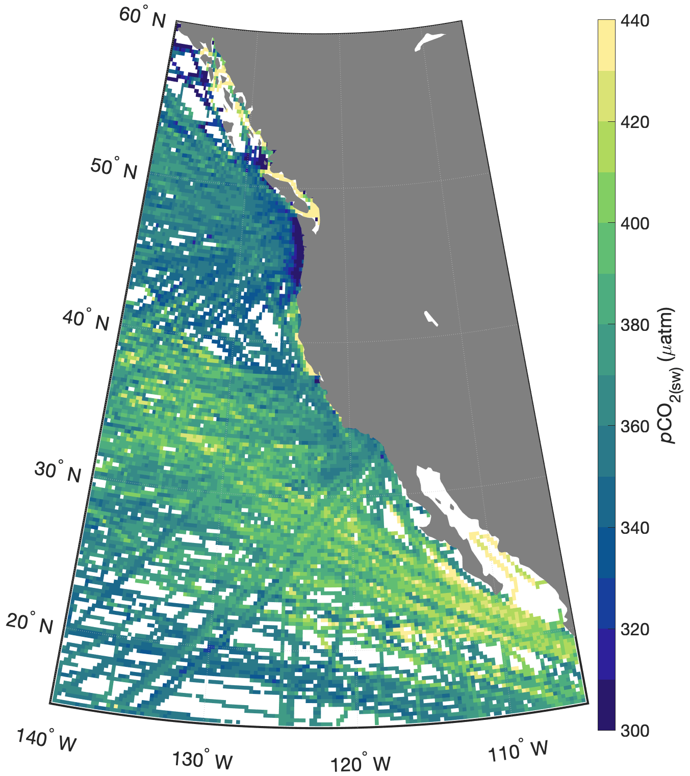
Figure 1Annual mean pCO2(sw) from the 0.25∘ resolution gridded dataset computed as an average over the monthly climatology from 1998 to 2020 for each grid cell. The two extremes of the color bar can represent pCO2(sw) values less than or greater than the color bar limits; the chosen range represents most of the values and emphasizes regional contrast.
2.2 Binning of pCO2(sw) observations
Sea surface CO2 partial pressure data were aggregated onto a 0.25∘ latitude by 0.25∘ longitude grid for each month from January 1998 to December 2020 using a bin-averaging procedure that consisted of computing the means (μ) and standard deviations (σ) of all observations of pCO2(sw) included within each grid cell. Observations prior to 1998 were excluded as an increase in data coverage occurs around the start of 1998 and the first full year of SeaWiFS chlorophyll observations (which are used in our procedure to fill gaps in the pCO2(sw) dataset) is 1998. For cases in which observations in a given grid cell originated from two or more platforms (e.g., cruises or autonomous assets), platform-weighted μ and σ were computed by first taking the means and standard deviations of all observations made by each platform, then taking the means of those values. This ensured that all platforms contributing observations to a given grid cell were weighted equally, mitigating unwanted biases toward high-resolution measurement systems (Sabine et al., 2013).
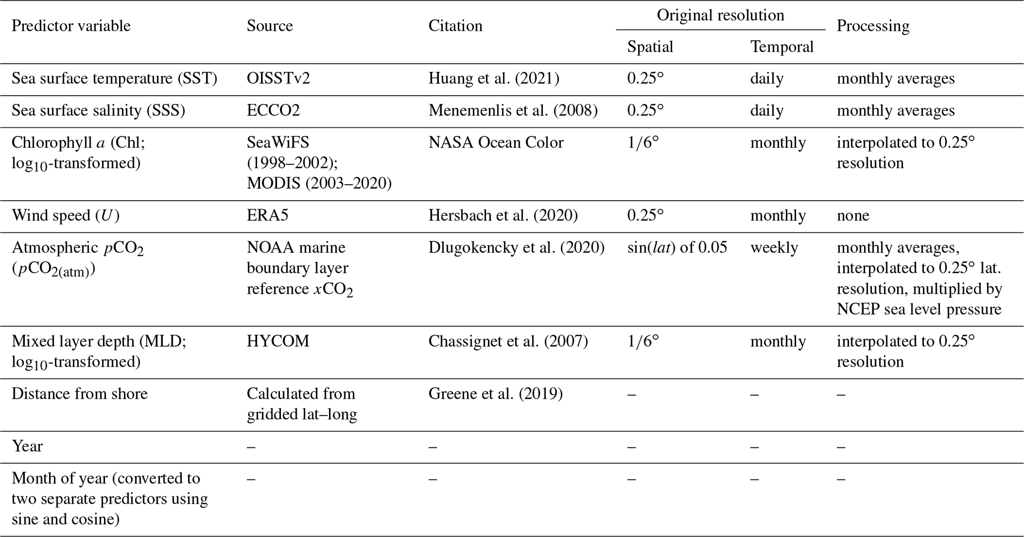
Table 1Sources of data for interpolation of surface pCO2. Chlorophyll a (Chl) and mixed layer depth (MLD) were log10-transformed to produce a distribution of values that was closer to normal before constructing the regression model. Gaps in CHL data were filled by linear interpolation over time within each grid cell (see Appendix A). Month of the year was transformed by cosine and sine functions to retain its cyclical nature.
This bin-averaging procedure is identical to the one followed by the SOCAT team for producing monthly datasets for coastal regions with 0.25∘ resolution as well as for open-ocean regions with 1∘ resolution (Sabine et al., 2013; Bakker et al., 2016). However, here we produced a monthly gridded dataset with 0.25∘ resolution for a region of the northeastern Pacific (15 to 60∘ N, 105 to 140∘ W) that spans both the coastal and open ocean. Means of pCO2(sw) from this gridded dataset (averages over the monthly climatology from 1998 to 2020 for each spatial grid cell) are shown in Fig. 1. Some of the apparent fine-scale spatial variability in this bin-averaged map is not indicative of true environmental conditions but originates from the combination of large temporal variability within each grid cell and uneven sampling of each grid cell across and within years. This form of temporal variability is exactly the kind of spurious result that advanced pCO2(sw) mapping techniques are intended to circumvent. Figure B1 shows the number of years containing an observation within each month of our gridded pCO2(sw) dataset. Unsurprisingly, temporal coverage is highest close to the coast, especially in the summer months.
2.3 Predictor variable acquisition and processing
Of the 4 014 844 grid cells that represent the surface ocean gridded in three dimensions at 0.25∘ resolution over 276 months (1998–2020) in the study region, just 1.25 % have an associated gridded pCO2(sw) value. To fill gaps in this dataset, relationships between pCO2(sw) and various predictor variables need to be determined. The predictor variables used in this study are primarily derived from satellite observations or reanalysis models due to the condition that they be resolved with temporal and spatial continuity across the study region and selected time span.
Predictor variables are intended to capture conditions that mechanistically influence pCO2(sw) (e.g., SST and atmospheric pCO2), serve as a proxy for mechanisms that influence pCO2(sw) (e.g., sea surface chlorophyll), or, in the case of temporal and spatial information, constrain additional patterned variability not captured by the mechanistic variables alone. The chosen predictor variables for this study (Table 1) have all been used before for pCO2(sw) gap-filling methods (e.g., Landschützer et al., 2014; Gregor et al., 2018; Denvil-Sommer et al., 2019; Watson et al., 2020); temporal and spatial predictors were included to ensure robust representation of pCO2(sw) seasonal cycles (Gregor et al., 2017). Included in Table 1 are the sources of each dataset, the original resolutions of each dataset, and the steps that were taken to process each dataset. Appendix A provides more detail about the acquisition and processing of the driver variables and includes figures showing annual means of selected variables.
2.4 Construction of nonlinear relationships using random forest regression
We used the random forest regression approach (Breiman, 2001) to identify relationships between pCO2(sw) and predictor variables in order to fill gaps in the gridded pCO2(sw) dataset. This method averages the results from a number of decision and/or regression trees (i.e., a “forest”) built on bootstrapped replicates of the dataset – which individually have low bias and high variance – to produce a final regression model with reduced variance (Hastie et al., 2009). RFR is the machine-learning method of choice for this study as early testing showed better performance than the SOM-FNN method in the northeastern Pacific. Further, RFR is less computationally expensive than fitting a neural network and has been shown to produce results comparable to the SOM-FFN approach in terms of overall performance (Gregor et al., 2017). It should be noted, however, that the two approaches differ mechanistically and therefore adapt to variability within a training dataset in different ways. Finally, while RFR has been explored more frequently in recent years as a method of spatiotemporal pCO2(sw) gap-filling both globally (Gregor et al., 2017, 2018) and regionally in the Gulf of Mexico (Chen et al., 2019), far fewer RFR-based pCO2(sw) products exist than neural-network-based products. So, this study provides a good opportunity to further demonstrate the utility of RFR for producing monthly fields of pCO2(sw), in this case on a regional scale in the northeastern Pacific.
Each decision tree within a random forest regression model is built on a different subset of the training dataset (that contains both the predictor variables and corresponding gridded pCO2(sw) values). This subset is generated by bootstrapping, in which a random set of training data points is selected with replacement – meaning the same data point can be selected more than once (Breiman, 1996). The number of data points in the bootstrapped dataset is equal to a defined fraction (InBagFraction in Table 2) of the original dataset; however, a fraction equal to 1 does not mean the bootstrapped dataset is identical to the original dataset because selection is made with replacement. Since each regression tree is built on a different subset of the training data, it will contain somewhat different relationships between the predictor variables and the corresponding gridded pCO2(sw) values.
Table 2Model parameters for the random forest regression. Parameter names are the default property names for the MATLAB TreeBagger class.
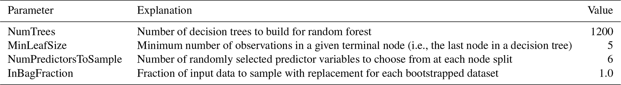
The process of building a decision tree begins at the top “node” of the tree with the values of a single predictor variable being used to split that tree's bootstrapped subset of the training dataset into two smaller subsets (not necessarily of equal size) containing the most similar pCO2(sw) observations (i.e., sets of pCO2(sw) observations with the smallest variance among them). These subsets are then further divided into progressively smaller sets of similar observations until either the variance among the pCO2(sw) observations in a node drops below a prescribed tolerance level or the number of observations in the node reaches the user-defined minimum (MinLeafSize in Table 2). To ensure that the algorithm does not always pick the same predictor variable (e.g., the one most highly correlated with pCO2(sw) overall) for the split at every node, we limit it to choosing from a different random subset of the predictor variables (equal in number to NumPredictorsToSample in Table 2) at each node. This introduces another “random” element into the tree-building process. The random forest contains a large number of these regression trees (NumTrees in Table 2) each built on a different, random bootstrapped subsample of the training data. Once the random forest is built, a set of predictor variables can be provided to the model and the average of the pCO2(sw) values provided by each regression tree is used as the pCO2(sw) prediction for that particular set of inputs.
We constructed an RFR model using the MATLAB TreeBagger function with the predictor variables given in Table 1 and the parameters given in Table 2, along with gridded pCO2(sw) values that were obtained as described in Sect. 2.1 and 2.2. To produce the northeastern Pacific random forest regressionpCO2(sw) product (RFR-CCS) that is the main result of this work (Sharp et al., 2022; https://doi.org/10.5281/zenodo.5523389), the full dataset of gridded pCO2(sw) values was used. For optimization and evaluation, subsets of the full dataset were used as described in the following sections.
2.5 Optimization of random forest regression model
The predictor variables used (Table 1) and the values for the model parameters (Table 2) were determined by iteratively optimizing the model performance. First, default model parameters were used to train an RFR model using a subset of the data for training (80 % of full dataset, distributed randomly across the space and time domains of interest) and a number of possible predictor variables: latitude, longitude, sea surface height, bottom depth, and those given in Table 1. During model selection, the generalization skill for the RFR model was assessed using a validation dataset comprised of 10 % of the full dataset, none of which was included in the training data. After the initial model fit, predictors with a “feature importance” (computed during the RFR fit) significantly lower than all other predictors were sequentially dropped (latitude, longitude, and sea surface height), and this did not substantially change the training or validation root mean squared error (RMSE). Remaining predictor variables were dropped one at a time for subsequent fits, and the goodness-of-fit and generalization skill of the model were assessed using the RMSE values calculated from applying the model to the training and validation datasets, respectively. The set of predictors with the lowest RMSE after dropping one predictor was carried into the next iteration. If removing a predictor did not increase the validation RMSE significantly, then that predictor was removed from the set of predictors (only bottom depth was dropped in this step). The final set of predictor variables is shown in Table 1.
Next, different values for model parameters (Table 2) were tried iteratively with the retained predictors to identify the optimal values, again by minimizing the RMSE of the validation dataset. Although lower values for the minimum terminal node size performed better in this analysis, additional testing indicated that retaining the default value of 5 was important to prevent overfitting. To determine the appropriate number of trees, we examined how the out-of-bag mean squared error changed as more and more trees were included in the random forest (up to 5000 trees) and selected a number of trees well past the point at which this error had stabilized (1200 trees). Finally, the remaining 10 % of the full dataset that was withheld from both the model training and model validation (i.e., the “test data”) was used to quantify the mapping uncertainties from the RFR approach (discussed further in Sects. 2.7 and 3.5). The predictor variable feature importances for the final RFR-CCS fit are given in Fig. B2.
2.6 Evaluation of random forest regression approach and resulting data product
Once predictor variables and model parameters were optimized, the skill of the RFR approach was further evaluated by splitting the full dataset into different subsets of training data and test data. Evaluation models (RFR-CCS-Evals) were constructed in three different ways: (1) by removing a random (20 %) subset of cruises and/or measurement platforms from the training data (repeated 10 times with different subsets removed each time; n=10), (2) by removing all observations from every fifth year from the training data (repeated five times such that data from every year was removed from one of the trials; n=5), and (3) by removing all moored autonomous pCO2(sw) measurements (i.e., discrete time series sites primarily located in the coastal ocean) from the training data (n=1). The first two strategies were relevant for assessing bulk error statistics for the method applied across the region and the third strategy for evaluating the ability of the RFR to represent local seasonal variability without the use of high-temporal-resolution mooring data. These RFR-CCS-Evals are distinct model variants that are only used for assessment; the final RFR-CCS model uses all available training data.
Each data split for an RFR-CCS-Eval was applied directly to SOCATv2021 observations, before bin-averaging the data according to the procedure given in Sect. 2.2; as a result, a gridded training dataset and a gridded test dataset were produced from each split. Data splits were performed in this way to ensure that autocorrelation among measurements from a specific platform did not bias the error statistics. Each split was repeated n times, and error statistics (bias, RMSE, and R2) from comparing pCO2(sw) predicted from the RFR-CCS-Eval models versus pCO2(sw) from the gridded test dataset were averaged.
The final RFR-CCS data product was evaluated through comparisons with gridded pCO2(sw) observations from SOCATv4 (Bakker et al., 2016) and pCO2(sw) observations from surface ocean moorings (Sutton et al., 2019). Of the surface ocean moorings within the study site that are not located within an inland sea and have available data from all 12 months of the year, four (CCE2, NH10, Cape Elizabeth, Châ bá) are located within 40 km of shore and one (CCE1) is about 215 km from shore. RFR-CCS was also compared to global-scale gap-filled pCO2(sw) products that are available in the region. Namely, we focused on the coastal multi-month pCO2(sw) product from Laruelle et al. (2017; i.e., L17) and the combined coastal and open-ocean pCO2(sw) climatology from Landschützer et al. (2020b; i.e., L20).
2.7 Uncertainty analysis
Uncertainty in pCO2(sw) for each grid cell was calculated according to the approach used by Landschützer et al. (2014, 2018) and Roobaert et al. (2019), in which total uncertainty in pCO2(sw) results from a combination of observational uncertainty, mapping uncertainty, and gridding uncertainty. Observational uncertainty (θobs) is uncertainty inherent to the original measurements of pCO2(sw) evaluated as the average of reported uncertainties in the observations from our training dataset, which are flagged by SOCAT with a dataset QC flag of A or B ( accuracy of 2 µatm or better) and of C or D ( accuracy of 5 µatm or better); we weighted θobs by the number of observations assigned each flag. Mapping uncertainty (θmap) is uncertainty contributed by the RFR mapping procedure and was evaluated as separate values for the coastal (< 400 km from shore) and open ocean (> 400 km from shore) using the mean of the root mean squared errors for a subset of test data (10 %) withheld from both the model training data (80 %) and model validation data (10 %) (see Sect. 2.5). Gridding uncertainty (θgrid) is uncertainty attributable to aggregating observations into monthly 0.25∘ resolution grid cells and was evaluated as separate values for the coastal and open ocean by taking the average unweighted standard deviation among pCO2(sw) values within each grid cell in which two or more platforms were represented. Grid cells with mooring observations were excluded from the θgrid calculation to avoid the high number of observations swamping the signal from other platforms. These three components were combined to obtain total pCO2(sw) uncertainty () applicable to each open-ocean grid cell and to each coastal grid cell:
Whereas represents the uncertainty in pCO2(sw) for a given grid cell in a given month, uncertainty averaged regionally or over time will not scale exactly with due to the spatial correlation of pCO2(sw) values and the autocorrelation features of the model error (e.g., Landschützer et al., 2014).
2.8 Calculation of CO2 flux
The flux of CO2 across the ocean–atmosphere interface () was calculated using a bulk formula:
where kw is the gas transfer velocity, K0 is the CO2 solubility constant, and ΔpCO2 is the difference between CO2 partial pressure in seawater and in the overlying atmosphere (pCO2(sw)−pCO2(atm)) The salinity- and temperature-dependent equations of Weiss (1974) were used to calculate K0.
Gas transfer velocities were parameterized using a quadratic dependence on wind speed (Wanninkhof, 1992):
where Γ660 is a gas exchange coefficient normalized to Sc = 660, U2 is the squared wind speed, and Sc is the Schmidt number for CO2. Our calculations used Γ660=0.276, which is a gas exchange coefficient that is specific to ERA5 reanalysis winds and scaled to a bomb-14C flux estimate of 16.5 cm h−1 (Fay et al., 2021). Sc was calculated using the fourth-order polynomial fit of Wanninkhof (2014). U was obtained from ERA5 reanalysis (Hersbach et al., 2020). Flux calculations used monthly averages of squared 3-hourly wind speeds to retain the influence of the quadratic wind term (Fay et al., 2021).
3.1 Evaluation by comparison to withheld data
As described in Sect. 2.6, training and test datasets were created by splitting the full dataset prior to bin-averaging. Evaluation models (RFR-CCS-Evals) were constructed by fitting RFR models using the various gridded training datasets. Values of pCO2(sw) predicted by RFR-CCS-Evals were compared to corresponding values from gridded test datasets. Error statistics (bias, RMSE, and R2) averaged over the n sets of evaluation tests are given in Table 3. When RFR-CCS is compared against all the gridded observations used to construct it, error statistics are predictably strong (last row in Table 3), with a mean bias of 0.00 µatm and an RMSE of 13.33 µatm (R2=0.93). These error statistics demonstrate the ability of the RFR model to fit the training data; the evaluation tests provide insight into the model's ability to predict independent data.
Table 3Error statistics for comparisons of predicted pCO2(sw) from evaluation models versus gridded pCO2(sw) from test datasets. The number of times each test was repeated is given by n; where n is greater than 1, different subsets of data were removed for each iteration of the test and error statistics are the mean of all iterations.
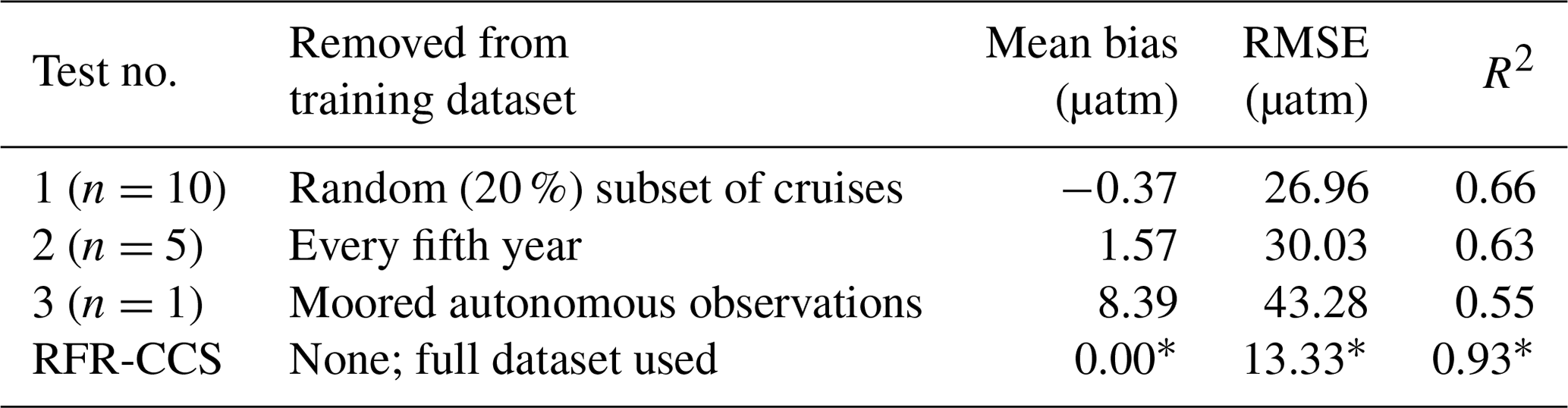
∗ These statistics represent model training statistics (i.e., evaluated with the same data used to train the model) rather than model validation statistics.
Tests 1 and 2 are good indicators of the overall skill of RFR-CCS. The mean absolute bias for each of those tests is less than 2 µatm, and the RMSEs are near or below 30 µatm. These error statistics can be compared with those of L17, who obtained biases with a mean of 0.0 and RMSEs ranging from 20.5 to 53.1 µatm (mean of 39.2 µatm) for independent evaluations of coastal pCO2(sw) values fit using the SOM-FFN method in 10 separate global subregions at 0.25∘ resolution. For an open-ocean comparison, Denvil-Sommer et al. (2019) obtained an RMSE of 15.86 for an independent evaluation of pCO2(sw) values fit using a similar neural network approach (LSCE-FFNN) for the subtropical North Pacific (18 to 49∘ N) at 1∘ resolution. The error statistics for our study region, which spans the coastal to open-ocean continuum on a finely resolved spatial grid, lie comfortably between those coastal and open-ocean comparison points.
Test 3 is a good indicator of how well the RFR approach is able to reproduce the values and seasonalities of coastal pCO2(sw) at fixed locations when mooring data at a given location are not provided as training data, as each of the moorings makes continuous pCO2(sw) measurements throughout the year and all but one of the mooring locations included in SOCATv2021 in this region are within 40 km of shore. The positive mean bias (8.39 µatm) suggests that RFR-CCS somewhat overestimates pCO2(sw) at grid cells corresponding to mooring locations, but this is strongly influenced by high biases at the Cape Elizabeth and Châ bá mooring locations (Table B1). The relatively high RMSE (43.28 µatm) is a result of higher variability in coastal grid cells compared to the open ocean; this is confirmed by a comparison to the offshore CCE1 mooring (Table B1), where the RMSE from the mooring-excluded RFR-CCS-Eval is just 10.5 µatm.

Figure 2Monthly values of pCO2(sw) from mooring observations (black), RFR-CCS (blue), the mooring-excluded RFR-CCS-Eval model (orange), and L17 (green). The envelope around the black line equals the standard deviation of all mooring observations within each month, representing the natural variability of the 3-hourly mooring measurements; the envelopes around the blue and orange lines represent the RFR-CCS and RFR-CCS-Eval results plus 1 standard uncertainty (43.6 µatm; Sect. 3.5); the envelope around the green line represents the L17 data product plus the RMSE of an independent data evaluation in the province associated with CCE2 (52.5 µatm; Table 3 of Laruelle et al., 2017; Province P7).
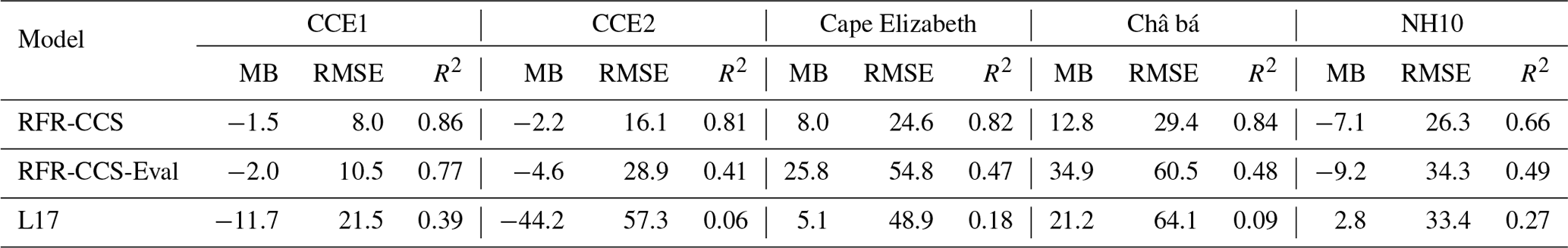
Figure 2 provides an example of one coastal mooring record (CCE2, which is positioned on the shelf break off the coast of Point Conception, CA, at 34.324∘ N, 120.814∘ W) compared to pCO2(sw) predicted in the corresponding grid cell (centered at 34.375∘ N, 120.875∘ W) by the mooring-excluded RFR-CCS-Eval model (Test 3) as well as the full RFR-CCS model. For comparison, pCO2(sw) in the same grid cell provided by the L17 coastal product is also shown. At the CCE2 mooring location, RFR-CCS reproduces mooring-observed monthly pCO2(sw) with a mean bias of −2.2 µatm and an RMSE of 16.1 µatm (R2=0.81). These error statistics are expected to be relatively favorable, as the RFR-CCS model is trained using mooring observations from CCE2. In contrast, the mooring-excluded RFR-CCS-Eval reproduces monthly mooring-observed pCO2(sw) at CCE2 with a mean bias of −4.6 µatm and an RMSE of 28.9 µatm (R2=0.41). This can be compared to the L17 coastal pCO2(sw) product, which reproduces monthly mooring-observed pCO2(sw) at CCE2 with a mean bias of −44.2 µatm and an RMSE of 57.3 µatm (R2=0.06). Notably, the mooring-excluded RFR-CCS-Eval captures pCO2(sw) variability at CCE2 more effectively than the L17 product, even though RFR-CCS-Eval was trained without mooring observations and the L17 training dataset (i.e., SOCATv4) includes CCE2 mooring observations through 2014. Similar results are obtained for comparisons to other mooring records (Table B1; Fig. B3), with RFR-CCS always producing the best error statistics (as expected) and RFR-CCS-Eval always producing a better R2 than L17, indicating that coastal seasonality at mooring locations is better captured by our regional random forest regression model, even when mooring observations themselves are not included in the model training. This is an important conclusion, especially in light of the recommendation by Hauck et al. (2020) that the inclusion of coastal areas and marginal seas in pCO2(sw) mapping methods will be critical for improving the ocean carbon sink estimate. If these areas are to be included, it is sensible to attempt to capture their unique modes of variability as accurately as possible.
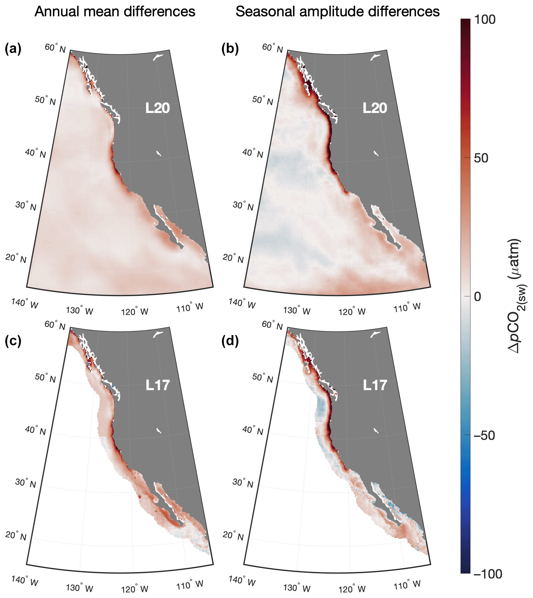
Figure 3Differences between annual means (a, c) and seasonal amplitudes (b, d) of pCO2(sw) from RFR-CCS-clim versus the L20 climatology (a, b; RFR-CCS-clim – L20) and versus a climatological average of the L17 product (c, d; RFR-CCS-clim – L17).
3.2 Evaluation by comparison to global pCO2(sw) products
Across the study area, values of pCO2(sw) from RFR-CCS were compared against corresponding values from L17 and L20. For temporal compatibility with L17 and L20, a climatology of average monthly values from RFR-CCS spanning 1998 to 2015 (RFR-CCS-clim) was created for these comparisons. Figure 3 shows mapped differences in annual means and seasonal amplitudes (calculated as the maximum climatological pCO2(sw) minus the minimum) of pCO2(sw) between RFR-CCS-clim versus L20 (top panels) and RFR-CCS-clim versus a climatological average of L17 (bottom panels); monthly mean differences in are given in Fig. B4.
The most notable feature of the annual mean difference maps is that RFR-CCS-clim produces much higher annual mean pCO2(sw) than both L17 and L20 in the nearshore coastal ocean and slightly higher pCO2(sw) in the remainder of the study area. Similarly, RFR-CCS-clim produces much higher seasonal variability than both L17 and L20 in the nearshore coastal ocean, especially north of about 34∘ N. On average, RFR-CCS-clim produces an area-weighted annual mean pCO2(sw) that is greater than L17 by 19.0 µatm and L20 by 8.4 µatm, as well as an area-weighted seasonal amplitude that is greater than L17 by 13.0 µatm and L20 by 5.6 µatm.
3.3 Evaluation by comparison to gridded observations of pCO2(sw)
Values of pCO2(sw) from RFR-CCS, L17, and L20 were compared against the SOCATv4 gridded pCO2(sw) data product. SOCATv4 was used in the development of the coastal L17 product, whereas SOCATv5 was used in the development of the open-ocean product for the merged L20 climatology, and SOCATv2021 was used in the development of RFR-CCS. Therefore, comparisons were made to both the gridded open-ocean observations (1∘ resolution) and gridded coastal observations (0.25∘ resolution) from SOCATv4 to include only data points that were available to the training of all three data products. To match the resolution of the gridded open-ocean observations from SOCATv4, aggregation from a 0.25∘ resolution grid to a 1∘ resolution grid was performed for RFR-CCS, RFR-CCS-clim, and L20. L17 was only compared to gridded coastal observations from SOCATv4 because the two are gridded to the same spatial resolution and cover the same coastally limited spatial domain.
Figure 4 shows two-dimensional histograms of bin-averaged differences between RFR-CCS-clim, L20, RFR-CCS, and L17, each compared against gridded observations from SOCATv4. For comparisons to climatological products (RFR-CCS-clim and L20), gridded SOCATv4 observations were averaged to a monthly climatology across 1998–2015 for consistency with the products. The regional RFR-CCS product and its climatology outperform both global SOM-FFN products: RFR-CCS-clim shows better agreement with gridded monthly means of observations from SOCATv4 than L20 (R2=0.85 versus R2=0.73), and RFR-CCS (within the coastally limited spatial domain of L17) shows better agreement with gridded observations from SOCATv4 than L17 (R2=0.96 versus 61). In particular, the two global products (L20 and L17) struggle to match pCO2(sw) values in the nearshore coastal ocean (within 100 km of the coast), indicated by dark blue cells in Fig. 4.
Mismatches between global pCO2(sw) products and observations in the nearshore coastal ocean are not unexpected, as regional error statistics for reconstructed global pCO2(sw) are typically larger than the global mean error statistics (Laruelle et al., 2017; Landschützer et al., 2020c), and it is generally more challenging to model pCO2(sw) in environments with high temporal and spatial variability, such as in the nearshore coastal ocean (Landschützer et al., 2014). This result emphasizes the importance of carefully addressing nearshore pCO2(sw) when constructing global products if one hopes to achieve an accurate representation of coastal ocean variability. This may be achieved (1) by using a greater number of model clusters for coastal ocean reconstructions (L17 uses just 10 biogeochemical clusters for the global coastal ocean), (2) by increasing the spatial and/or temporal resolution of pCO2(sw) data products to better account for small-scale variability (Gregor et al., 2019), (3) by carefully accounting for mismatches between the temperature (and salinity) at which pCO2(sw) is measured versus that at which it is reported in surface data products (Ho and Schanze, 2020; Watson et al., 2020), or (4) by taking an ensemble approach to pCO2(sw) gap-filling to reduce errors overall, especially in undersampled regions (Gregor et al., 2019; Fay et al., 2021). Ultimately, it will be critical to continue to expand our observational capabilities by means of shipboard underway systems (Pierrot et al., 2009), uncrewed surface vehicles (Meinig et al., 2015; Sutton et al., 2021), biogeochemical Argo floats (Roemmich et al., 2019), moored buoys (Sutton et al., 2019), and other platforms, as well as to make strides toward incorporating these novel measurements into pCO2(sw) gap-filling schemes (Gregor et al., 2019; Djeutchouang et al., 2022).
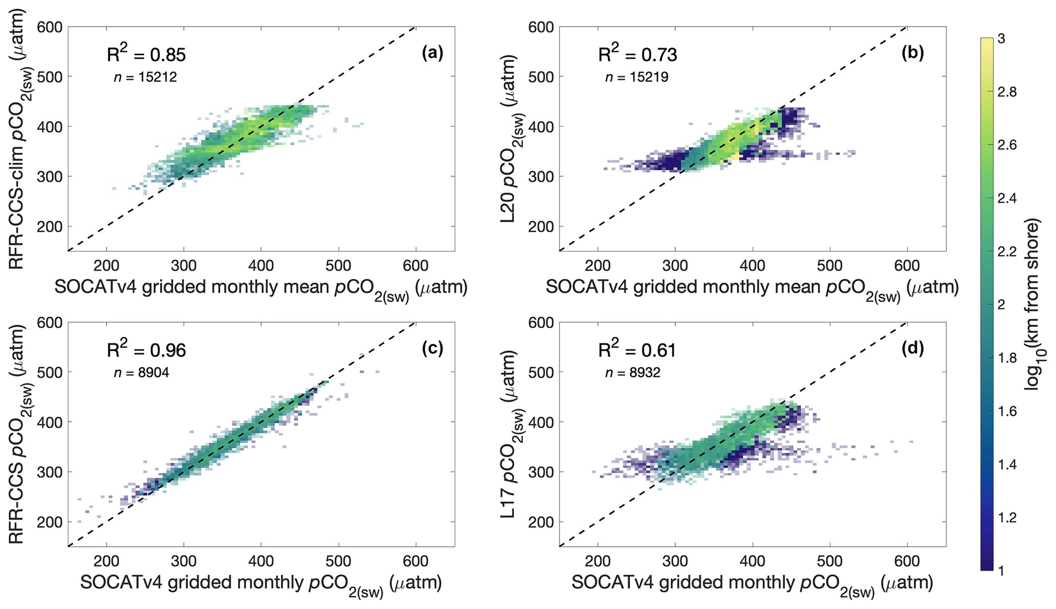
Figure 4Two-dimensional histograms showing bin-averaged comparisons of pCO2(sw) from (a) RFR-CCS-clim and (b) L20 to SOCATv4 gridded observations that have been averaged to a climatology, as well as comparisons of pCO2(sw) from (c) RFR-CCS and (d) L17 to SOCATv4 gridded monthly observations in the coastally limited spatial domain of L17. Grid cells are color-coded by the average base-10 logarithm of distance from shore (km) of the observations included within each bin; the transparency of each grid cell is set by the relative number of observations within each bin.
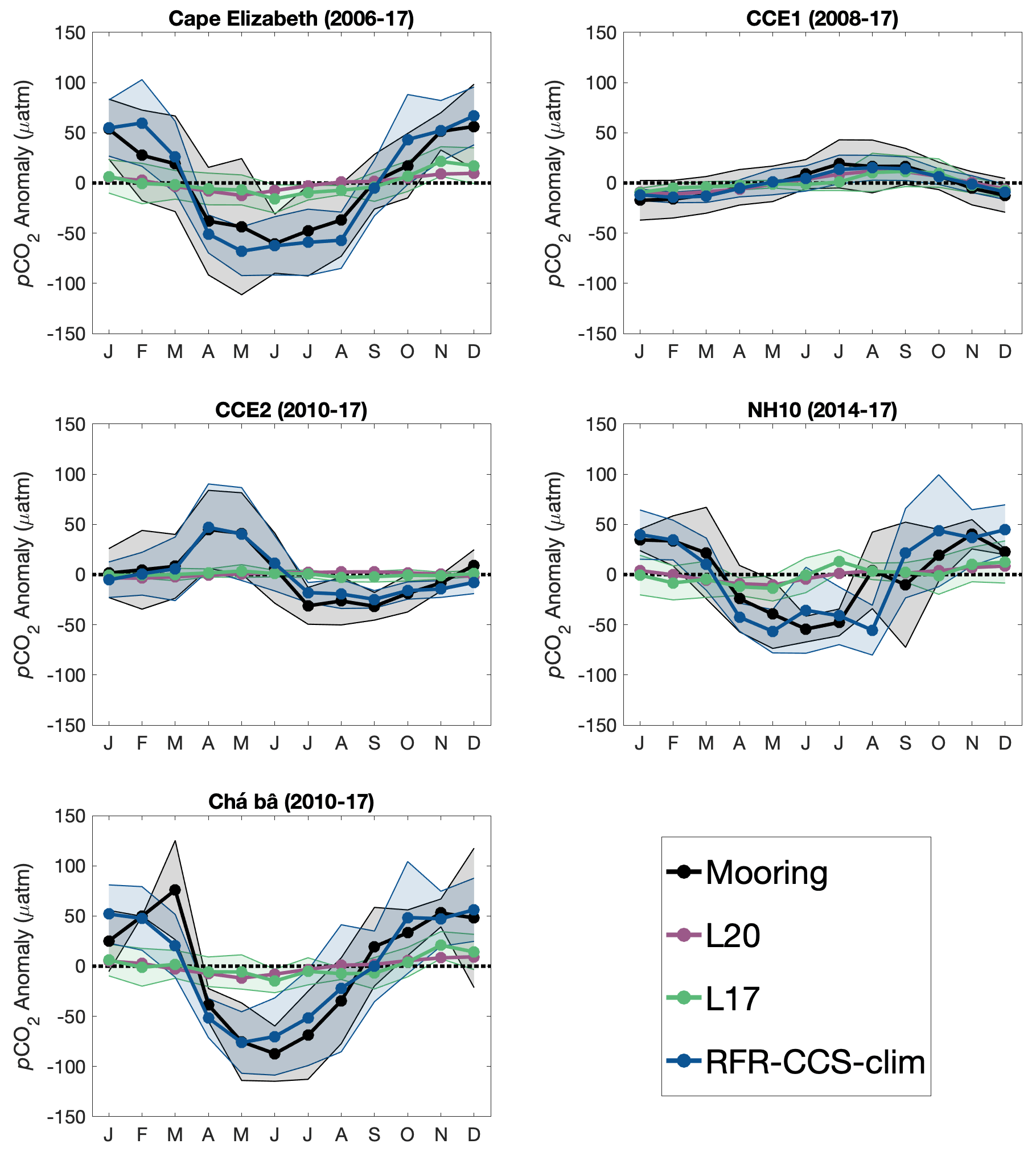
Figure 5Climatological mean pCO2(sw) from five NOAA ocean moorings and the corresponding grid cells in RFR-CCS-clim, L20, and a climatological average of L17. Shading represents the standard deviation of all monthly values for each mooring or data product.
3.4 Evaluation by comparison to seasonal observations of pCO2(sw) at ocean moorings
Values of pCO2(sw) from RFR-CCS-clim, L17, and L20 were compared against monthly climatologies from mooring observations to evaluate how well each product captured seasonal variability at fixed time series sites. Figure 5 shows climatologies of mooring-observed pCO2(sw) (each averaged over available years and normalized to their annual mean) compared to pCO2(sw) from RFR-CCS-clim, L20, and climatological monthly averages of L17 (each normalized to their annual mean) in the grid cell corresponding to the mooring location. Overall, RFR-CCS-clim does a much better job of capturing the variability in mooring observations than either L17 or L20 (Table 4).
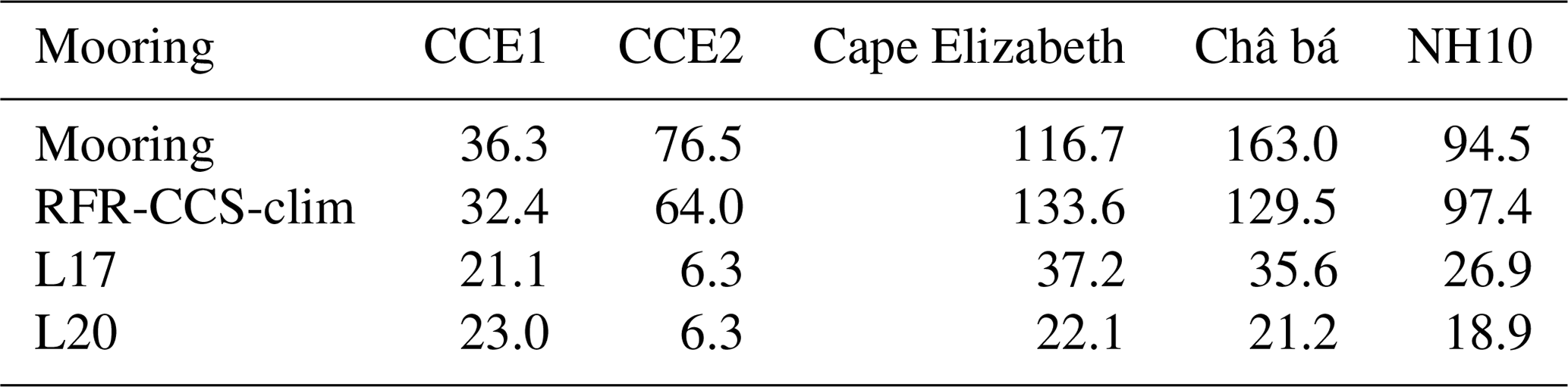
Table 4Seasonal amplitudes of pCO2(sw) (µatm) from mooring observations and corresponding grid cells of climatological averages (from 1998–2015) of RFR-CCS-clim, L17, and L20.
3.5 Uncertainty calculations
Three components comprised the estimate of uncertainty for pCO2(sw) values from RFR-CCS: observational uncertainty (θobs), mapping uncertainty (θmap), and gridding uncertainty (θgrid). According to the procedure detailed in Sect. 2.7, θobs was calculated as 3.3 µatm, θmap as 4.4 µatm for the open ocean and 35.3 µatm for the coastal ocean, and θgrid as 3.7 µatm for the open ocean (n=268) and 25.1 µatm for the coastal ocean (n=889). These three components were combined to obtain total pCO2(sw) uncertainty () according to Eq. (2), resulting in equal to 6.6 µatm for the open ocean and 43.4 µatm for the coastal ocean. The open-ocean value determined through this analysis compares well with the grid-level uncertainty estimated in open-ocean grid cells by Landschützer et al. (2014), which ranged from 8.6 to 17.7 µatm for different regions. The large coastal uncertainty value emphasizes the high degree of variability in monthly pCO2(sw) near ocean margins.
As noted in Sect. 2.7, uncertainties reported here are appropriate for a given grid cell (i.e., monthly 0.25∘ latitude by 0.25∘ longitude bin). Values averaged over time or over larger regions will have reduced pCO2(sw) (and CO2 flux) uncertainties due to the spatiotemporal correlation of pCO2(sw) and the autocorrelation features of the model error (e.g., Landschützer et al., 2014).
3.6 Spatial and seasonal patterns of sea surface pCO2
In the open ocean, relatively high pCO2(sw) values can be observed off southern Baja California (Fig. 6a) and extending toward the northwest, especially during summer months and into autumn (Fig. 7) when higher sea surface temperatures drive higher pCO2(sw) (Nakaoka et al., 2013). This area also corresponds to low chlorophyll (Fig. A2) and the lowest wind speeds across the study region (Fig. A4), suggesting that a lack of nutrient delivery from deep convection may be limiting biological production, also driving high pCO2(sw). Relatively low open-ocean pCO2(sw) values can be observed in the northern part of the study region from about 45 to 60∘ N (Fig. 6a). Wintertime cooling drives low pCO2(sw) in this area, though that effect is compensated for by dissolved inorganic carbon (DIC) brought to the surface by deep winter mixing (Ishii et al., 2014). Figure B5 illustrates competing effects between temperature and winds by displaying correlations between SST and pCO2(sw), which are mainly positive below 50∘ N, and between wind speed and pCO2(sw), which are mainly positive above 50∘ N.
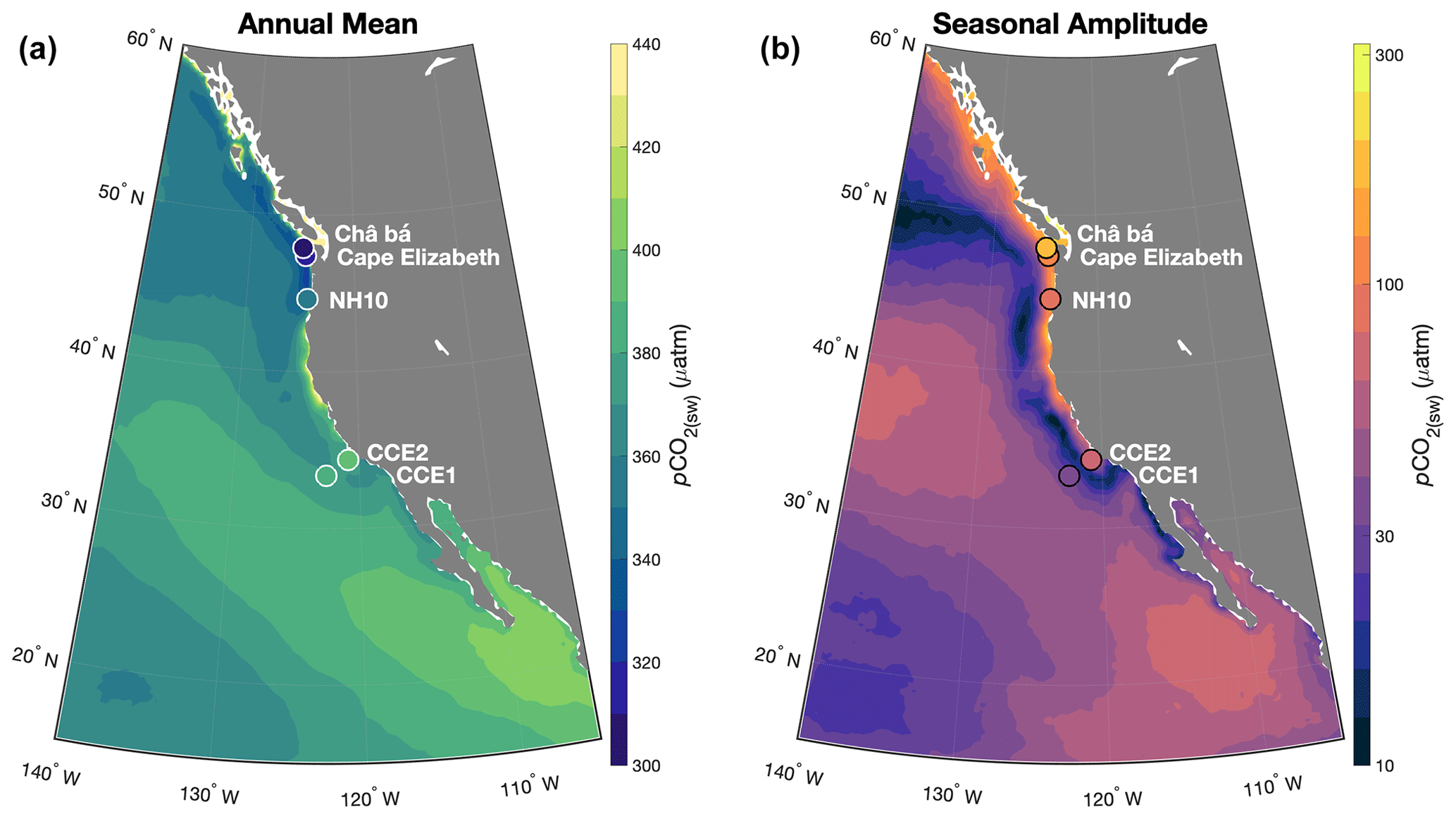
Figure 6Annual mean pCO2(sw) (a) and the seasonal amplitude of pCO2(sw) (b) from RFR-CCS. Also shown are annual mean pCO2(sw) and the seasonal amplitude of pCO2(sw) measured at ocean mooring locations.
In the summer, high biological production in the northern portion of the study region (Fig. A2) removes DIC, keeping pCO2(sw) relatively low. This low-pCO2(sw) region extends southward along the California coast to about 34∘ N between both offshore and nearshore high-pCO2(sw) waters. The southward extension of the low-pCO2(sw) region is consistent with what we know about the dynamics of the CCS: a narrow band of nearshore waters is high in DIC in the spring and summer due to the direct effects of wind-driven upwelling (Fig. 7), but a wider band of waters farther offshore is lower in DIC due to drawdown by high biological production stimulated by nutrients delivered to the euphotic zone by upwelling (Hales et al., 2005; Fassbender et al., 2011; Fiechter et al., 2014; Turi et al., 2014).
In the coastal ocean, high pCO2(sw) occurs in the central CCS (∼ 34 to ∼ 42∘ N), with values of 400 µatm or greater beginning in April off Pt. Conception (34∘ N) and propagating northward to around Cape Arago (43∘ N) through October (Fig. 7). This corresponds to the latitudinal band of the CCS with the strongest and most consistent equatorward winds (Huyer, 1983), which induce upwelling of CO2-rich subsurface waters by wind-driven Ekman transport very near the coast and wind-stress-curl-driven Ekman pumping farther offshore (Checkley and Barth, 2009). This nearshore band of high summertime pCO2(sw) has been previously reported by observational (Hales et al., 2012) and modeling (Fiechter et al., 2014; Turi et al., 2014; Deutsch et al., 2021) studies. It corresponds to naturally low surface pH values and aragonite saturation states, which will be exacerbated by increasing atmospheric CO2 concentrations (Gruber et al., 2012; Hauri et al., 2013), with likely deleterious effects for calcifying organisms (Feely et al., 2008).
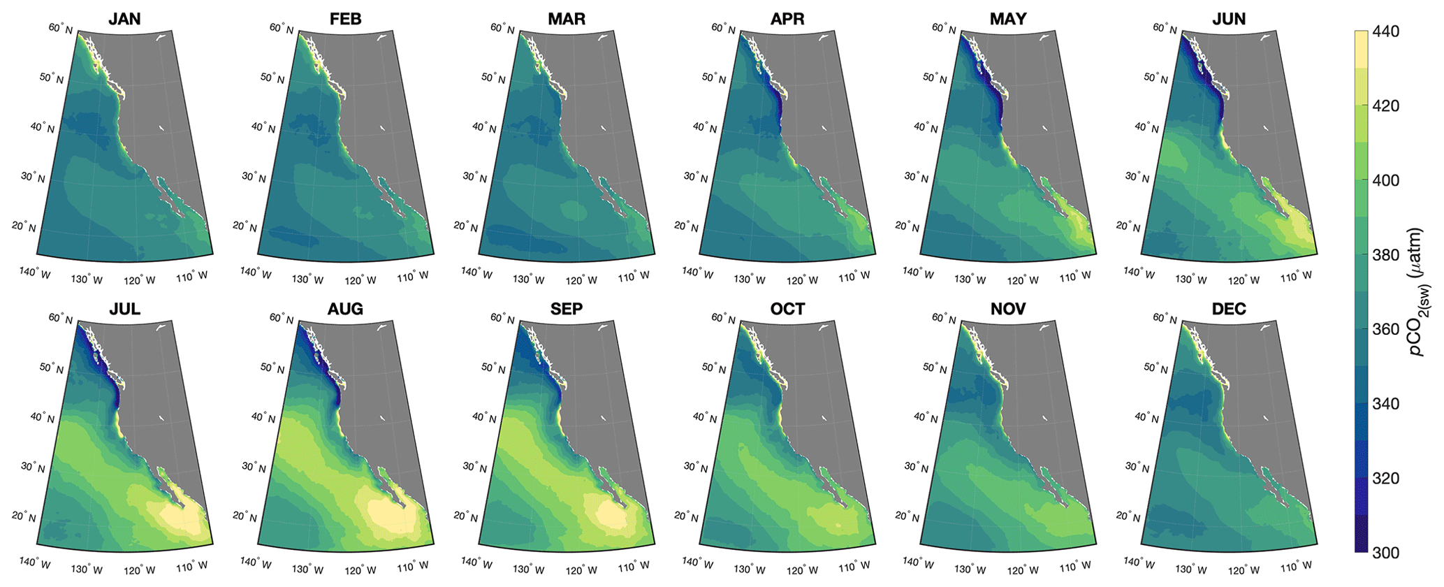
Figure 7Monthly mean pCO2(sw) fields from RFR-CCS.
Relatively low coastal pCO2(sw) values (340 µatm or lower) develop during April off the coasts of Oregon, Washington, and Vancouver Island and propagate northward toward southern Alaska through September (Fig. 7). Low summertime pCO2(sw) in the northern CCS (∼ 42 to ∼ 50∘ N) has been demonstrated before (Hales et al., 2005, 2012; Evans et al., 2011; Fassbender et al., 2018) and corresponds to the weaker and more variable equatorward winds in summer in the northern CCS (Checkley and Barth, 2009) as well as the effect of DIC drawdown by high primary productivity, which offsets upwelling-induced increases in pCO2(sw). Primary productivity in the northern CCS can be enhanced relative to the rest of the CCS due to factors like riverine nutrient delivery and distribution, submarine canyon-enhanced upwelling, and physical retention of phytoplankton blooms (Hickey and Banas, 2008).
The coastal ocean from Vancouver Island northward is a high-pCO2(sw) region from October to March (Fig. 7), which is broadly consistent with observations of high pCO2(sw) in the western Canadian coastal ocean during autumn and winter (Evans et al., 2012, 2022). This high pCO2(sw) is perhaps due to the influence of deep tidal mixing (Tortell et al., 2012) and wintertime light limitation of DIC drawdown by primary production. The northern coastal area shifts to a low-pCO2(sw) region from April to September, again consistent with observations (Evans et al., 2012, 2022) and likely reflecting surface DIC drawdown by primary production in the region (Ianson et al., 2003).
The coastal ocean from the Southern California Bight (SCB) southward along Baja California (∼ 22 to ∼ 34∘ N) shows relatively low pCO2(sw) seasonality (Fig. 6b). In this region, pCO2(sw) is generally lower than in offshore waters of the same latitude, which matches previous results well (Fig. 6a; Hales et al., 2012; Deutsch et al., 2021). One exception is directly off the southern tip of Baja California, where especially high summertime pCO2(sw) is observed. This may in part reflect the tendency for wind-driven upwelling to bring significant amounts of CO2-rich subsurface waters to the surface just south of major topographic features (Van Geen et al., 2000; Friederich et al., 2002; Fiechter et al., 2014). Coastal pCO2(sw) within the Gulf of California (GoC) appears to be strongly influenced by thermally induced seasonal effects, though the lack of observational data coverage in the GoC within SOCATv2021 (Fig. 1), especially within the nonsummer months (Fig. B1), may mask more dynamic variability.
The seasonal amplitude of pCO2(sw) (Fig. 6b) exhibits interesting variation in the central and northern CCS. Here, nearshore seasonality is extremely high due to dominant effects from upwelling and primary production; however, seasonality farther offshore is extremely low, likely due to compensating effects by thermally driven changes to pCO2(sw) (high temperature in summer increases pCO2(sw), low temperature in winter decreases pCO2(sw)) and biologically or physically driven changes to pCO2(sw) (high primary production in summer decreases pCO2(sw), deep mixing in winter increases pCO2(sw)). Elsewhere, a hotspot of high seasonality exists offshore around 40∘ N, possibly due to thermal control of pCO2(sw) without strong biophysical compensatory effects.
3.7 Carbon uptake in the RFR-CCS domain
A recently published data product (SeaFlux; Gregor and Fay, 2021) described by Fay et al. (2021) harmonizes calculations of global CO2 flux by standardizing the areas covered by different global pCO2(sw) products and by scaling the gas exchange coefficient to different wind products. As part of this procedure, the L20 climatology is used to fill spatial gaps in some of the pCO2(sw) products. As we have demonstrated here, filling gaps with this climatology may result in an underestimate of the seasonal pCO2(sw) cycle in certain locations, especially nearshore (Fig. 5). For comparison we calculate monthly CO2 flux in our study region from SeaFlux and from RFR-CCS, resulting in the monthly climatologies shown in Fig. 8.
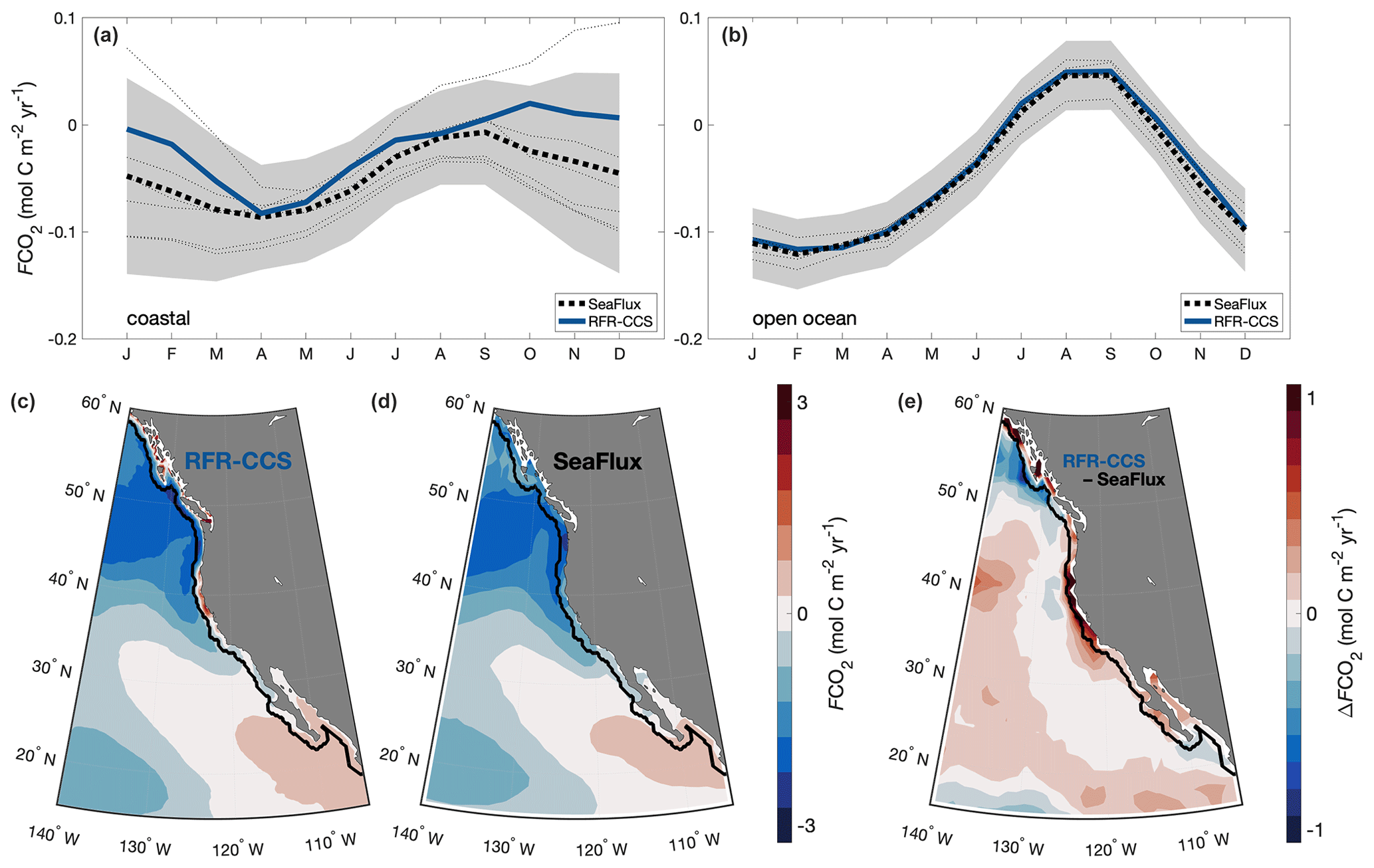
Figure 8Monthly CO2 flux per unit area for the nearshore coastal (a) and open-ocean (b) portions of the RFR-CCS domain calculated from the SeaFlux ensemble average (dotted black line; individual products in thin dotted lines) and from RFR-CCS (solid blue line). The grey shaded area represents variability in SeaFlux pCO2(sw) products calculated as plus and minus 1 standard deviation. Also shown is the spatially distributed CO2 flux per unit area calculated from RFR-CCS (c) and from SeaFlux (d), as well as the difference between them (e). Red in panels (c) and (d) indicates net release of CO2 to the atmosphere, whereas blue indicates net uptake of CO2; in panel (e), red indicates where the RFR-CCS CO2 flux per unit area is greater and blue where the SeaFlux CO2 flux per unit area is greater. The solid black line denotes the boundary between the nearshore coastal (a) and open ocean (b) calculated as 100 km from the coast. All calculations are performed using ERA5 winds and an identical gas exchange coefficient (Γ660=0.276).
Overall, the SeaFlux ensemble (with ERA5 winds) suggests an oceanic uptake of 69.2 Tg C yr−1 for the RFR-CCS domain between 1998 and 2019 (inclusive) compared to an uptake of 60.0 Tg C yr−1 calculated from RFR-CCS. Of the excess 9.2 Tg C yr−1 uptake from SeaFlux, 5.7 Tg C yr−1 comes from the open ocean and 3.5 Tg C yr−1 from the nearshore coastal ocean (within 100 km of the coast). Given that the nearshore coastal ocean only comprises about 9 % of the RFR-CCS region yet ∼ 38 % of the discrepancy, the discrepancy in coastal uptake is more significant on a per area basis than the open-ocean discrepancy, as can be observed visually in Fig. 8. This discrepancy may reflect more coastal outgassing captured by RFR-CCS than the SeaFlux ensemble, consistent with the annual mean differences shown in Fig. 3a and c. Still, the RFR-CCS results do lie within the variability of SeaFlux pCO2(sw) products (Fig. 8a and b).
3.8 Effect of sporadic sampling on coastal CO2 flux calculations
RFR-CCS includes pCO2(sw) values for the coastal and offshore ocean in the northeastern Pacific that are representative of monthly conditions. However, air–sea carbon dioxide exchange, which is driven by the difference between oceanic and atmospheric pCO2, operates on shorter timescales. It has been demonstrated in the past that inadequate sampling frequency can be a significant factor biasing CO2 flux () estimates (e.g., Monteiro et al., 2015).
To demonstrate this potential bias, Fig. 9 shows at the CCE2 mooring over the course of 2015 (1) calculated from RFR-CCS monthly pCO2(sw) matched to NOAA marine boundary layer monthly pCO2(atm) and monthly averages of squared 3-hourly ERA5 winds (blue), (2) calculated from 3-hourly mooring measurements of pCO2(sw) and pCO2(atm) matched to squared 3-hourly ERA5 winds (grey), and (3) as the 1-standard-deviation envelope obtained by the following Monte Carlo process: assigning one randomly selected pair of 3-hourly mooring measurements of pCO2(sw) and pCO2(atm) from each month as the monthly values, matching them with squared 3-hourly ERA5 winds to calculate , and repeating this 100 000 times to obtain statistically meaningful values (green).
The values provided by the 3-hourly mooring measurements are as close as possible to the true flux. Those provided by RFR-CCS are a best-case scenario for monthly flux approximations in the absence of continuous measurements (because the RFR model was trained on monthly mean pCO2(sw) values from 3-hourly observations at CCE2). Those provided by the Monte Carlo analysis provided reasonable ranges of that might be obtained from sporadic sampling of one measurement per month without the benefit of an advanced interpolation routine like RFR-CCS. The annual calculated from RFR-CCS (−0.26 mol C m−2 yr−1) agrees fairly well with that from the 3-hourly mooring measurements (−0.18 mol C m−2 yr−1). The smaller uptake from the mooring measurements likely reflects the effect of transient outgassing events in the spring and summer, when positive ΔpCO2 coincides with high wind speeds. The range from the Monte Carlo analysis (−0.00 to −0.36 mol C m−2 yr−1) highlights the variety of outcomes in calculated that might result from sporadic sampling in the coastal ocean, representative of a region with no high-resolution mooring measurements that may be observed by a ship's underway system only a few times a year.
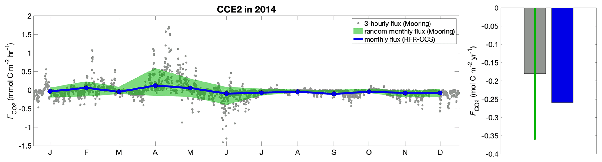
Figure 9Hourly flux of CO2 across the air–sea interface () calculated from 3-hourly mooring observations (grey), monthly values from RFR-CCS (blue), and the 1-standard-deviation envelope of a Monte Carlo analysis (n=100 000) whereby one randomly selected 3-hourly mooring observation from each month is selected to represent that month (green). The bar chart on the right gives annual based on 3-hourly mooring observations (−0.18 mol C m−2 yr−1) and RFR-CCS (−0.26 mol C m−2 yr−1), along with the uncertainty in annual from mooring measurements based on the Monte Carlo analysis (−0.00 to −0.36 mol C m−2 yr−1).
In large portions of the open ocean, low temporal variability and high spatial correlation mean that the aliasing problem may be a relatively low-priority concern for calculations of from sporadic pCO2(sw) measurements (Bushinsky et al., 2019). However, the dynamic coastal ocean is dominated by processes that influence pCO2(sw) and on short spatial and temporal scales, making observational frequency a significant factor that can bias annual calculations. This bolsters the case for the expansion and enhancement of coastal carbon observing systems even with pCO2(sw) gap-filling methods, such as the one described here, at our disposal.
The RFR-CCS data product (Sharp et al., 2022) is available as a NetCDF and MATLAB file at https://doi.org/10.5281/zenodo.5523389.
MATLAB code used to process data and create figures included in this paper is provided at https://github.com/jonathansharp/RFR-CCS (last access: 1 April 2022) and https://doi.org/10.5281/zenodo.6484875 (Sharp, 2022). The majority of this code is also compatible with the open-source software GNU Octave.
This work presents a data product, called RFR-CCS, of surface ocean pCO2 in the California Current System and surrounding ocean regions. RFR-CCS was constructed from pCO2(sw) observations in the Surface Ocean CO2 Atlas version 2021 (Bakker et al., 2016), which were related to predictor variables (Table 1) using a random forest regression approach. Validation exercises (Table 3) reveal that this approach is able to predict independent pCO2(sw) values with a skill commensurate with expectations (mean bias near zero and RMSE ≈ 30 µatm), considering the highly variable coastal ocean comprises a large portion of the study region.
RFR-CCS captures variability in pCO2(sw) in the northeastern Pacific, especially at coastal time series locations, more effectively than global-scale data products of pCO2(sw). This is evident through comparisons to gridded monthly observations in the SOCAT database (Fig. 4), to monthly observations at fixed mooring sites (Figs. 2 and B3; Table B1), and to seasonal amplitudes of pCO2(sw) measured at those moorings (Fig. 5; Table 4). The improvements made by RFR-CCS mainly represent the enhanced ability of regional data fits to capture local-scale variability compared to global data fits. Going forward, perhaps global-scale gap-filled pCO2(sw) products that include a clustering step would benefit from the creation of a greater number of clusters in the coastal ocean, allowing for more robust reconstruction of local variability. Improvements detailed here may also be due to the flexibility of RFR in capturing multiple different length scales of variability (Gregor et al., 2017), which may make the method especially useful for regions that span both the coastal and open ocean. The CCS is also particularly data-rich, and this work demonstrates the excellent resolution of nearshore variability that can be achieved in gap-filled pCO2(sw) products when coastal observing systems are sustained over time. Examination of the spatiotemporal distribution of pCO2(sw) observations contained in the SOCAT database (Bakker et al., 2016; http://www.socat.info, last access: 7 March 2022) suggests that analyses similar to this one could be effective for other coastal regions around North America, the western North Pacific, and the eastern North Atlantic. However, different predictor variable–pCO2(sw) relationships are likely to exist in these distinct ocean regions since each has a unique physical and biogeochemical setting.
Spatial and seasonal patterns of pCO2(sw) revealed by RFR-CCS reflect interactions of physical and biological processes that differ substantially with latitude, season, and distance from shore (Figs. 6 and 7). For example, high annual mean pCO2(sw) in a narrow band of the central coastal CCS reflects spring and summer upwelling; low annual mean pCO2(sw) and CO2 uptake in the northern coastal CCS and the offshore CCS in general reflects CO2 drawdown by primary production, largely stimulated by nutrients delivered by coastal upwelling. Generally, across the study region, interpretations of pCO2(sw) variability and the processes that drive it coincide with local-scale explanations in the coastal environment, suggesting high heterogeneity in coastal carbon cycling.
Finally, in the context of sea surface pCO2 gap-filling strategies, this study highlights important factors that should be considered when working in coastal areas or regions that span the coastal to open-ocean continuum. For one, although a global gap-filled product may demonstrate mean annual values and average seasonal amplitudes of pCO2(sw) that represent a broad region effectively, this does not mean that local-scale variability within that region has been captured just as well. Data-rich regions like the CCS confirm this notion, especially when variability at fixed time series sites like moored autonomous platforms is considered. Misrepresentation errors of this nature are especially concerning in dynamic nearshore environments, where local-scale processes can result in surface biogeochemical characteristics that change rapidly over short timescales. These rapid changes can have direct consequences for local biological responses and for CO2 flux, both of which operate on relatively short timescales. To address potential errors associated with misrepresentation of pCO2(sw) variability, the spatiotemporal coverage of carbon observing systems must be improved, especially at ocean margins. Further, innovative implementation and assessment of machine-learning approaches (Gregor et al., 2017; Gloege et al., 2021), biogeochemical models (DeVries et al., 2019; Friedlingstein et al., 2020), and ensemble approaches (Lebehot et al., 2019; Fay et al., 2021) should continue to be explored to best leverage the existing data.
SST (Fig. A1) was obtained from the NOAA daily Optimum Interpolation Sea Surface Temperature (OISST) analysis product (Reynolds et al., 2007; Huang et al., 2021). This data product combines satellite and in situ observations of SST using an optimum interpolation (OI) technique, providing daily SST values at 0.25∘ resolution. We averaged daily gridded SST values from OISSTv2.1 for each month from 1998 to 2020 to obtain the required monthly 0.25∘ resolution datasets to match with our gridded pCO2.
Sea surface salinity (SSS) was obtained from the NASA Estimating the Circulation and Climate of the Ocean (ECCO) project. The ECCO2 state estimate (Menemenlis et al., 2008) uses a Green's function approach (Menemenlis et al., 2005) to make optimal adjustments to parameters, initial conditions, and boundary conditions of a general circulation model to produce a daily ocean state estimate. We averaged daily gridded SSS values from the ECCO2 state estimate for each month from 1998 to 2020 to obtain the required monthly 0.25∘ resolution datasets to match with our gridded pCO2.
Sea surface chlorophyll a concentration estimates (Chl; Fig. A2), based on Sea-Viewing Wide Field-of-View Sensor (SeaWiFS) and Moderate Resolution Imaging Spectroradiometer (MODIS) satellite data, were obtained from the Oregon State University (OSU) Ocean Productivity website (http://www.science.oregonstate.edu/ocean.productivity, last access: 16 June 2021). The OSU Ocean Productivity website provides both monthly and 8 d Chl files at either ∘ or ∘ resolution. We obtained monthly ∘ resolution files for 1998–2002 (SeaWiFS-based) and 2003–2020 (MODIS-based) and interpolated each to a 0.25∘ resolution grid using a standard two-dimensional linear interpolation for each monthly file. For high-latitude wintertime gaps in the Chl datasets, we interpolated Chl for each grid cell through time using one-dimensional linear interpolation when observations in the previous and subsequent month were available. To avoid anomalous values at the beginning and end of the time series, empty grid cells were filled with nearest-neighbor interpolation when a previous or subsequent observation was not available (Fig. A3). Chl was log10-transformed to produce a distribution of values that was closer to normal before constructing the regression model.
Wind speed data (Fig. A4) were obtained from the ERA5 reanalysis product (Hersbach et al., 2020), produced by the European Centre for Medium-Range Weather Forecasts (ECMWF). The ERA5 atmospheric reanalysis provides a detailed record of atmospheric parameters from 1950 to the present day. We obtained monthly, 0.25∘ resolution wind speed data at 10 m above the surface from the Copernicus Climate Change Service (C3S) Climate Data Store (CDS). Wind speed (U) was calculated from its vector components (north–south wind, vw, and east–west wind, uw).
Atmospheric CO2 partial pressure (pCO2(atm)) was obtained from the NOAA marine boundary layer (MBL) reference (Dlugokencky et al., 2020). This data product is derived from weekly air samples of atmospheric CO2 mole fraction (xCO2) at a subset of sites from the NOAA Cooperative Global Air Sampling Network. The product is provided as weekly latitudinal averages with a resolution of sin(lat) = 0.5. We interpolated weekly xCO2 values to monthly xCO2 values relative to the middle of each month. To convert xCO2 to pCO2(atm), xCO2 was multiplied by monthly sea level pressure (P) from NCEP reanalysis, which was corrected for water vapor pressure (VP) as described by Dickson et al. (2007).
Mixed layer depths (MLDs), based on output from the Hybrid Coordinate Ocean Model (HYCOM) (Chassignet et al., 2007), were obtained from the OSU Ocean Productivity website. We obtained monthly ∘ resolution MLD files and interpolated each to a 0.25∘ resolution grid using a standard two-dimensional linear interpolation for each monthly file. MLD was log10-transformed to produce a distribution of values that was closer to normal before constructing the regression model.

Figure A1Gridded means of SST from satellite observations from 1998–2020.

Figure A2Gridded means of chlorophyll a concentration from satellite observations from 1998–2020.
Distance from shore (Dist.) for each grid cell was calculated using the dist2coast.m function from the Climate Data Toolbox for MATLAB (Greene et al., 2019), applied to each latitude–longitude grid cell. That function accepts input of latitude and longitude coordinates and returns the great circle distance to the nearest coastline.
Year (yr) was normalized to an epoch of 1997 (i.e., yrnorm = yr – 1997). Month of year (mn) was transformed into two separate predictor variables (mnsin and mncos) using sine and cosine functions to maintain its cyclical nature (after Gregor et al., 2018).
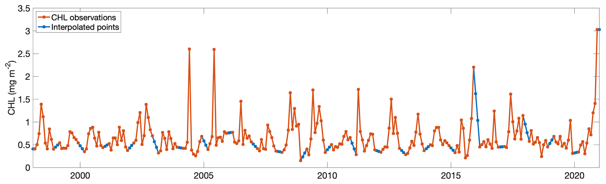
Figure A3Sea surface chlorophyll concentration at 55∘ N, 135∘ W. Data from satellite observations are in orange and interpolated data are in blue.
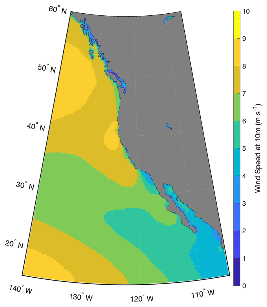
Figure A4Gridded means of wind speed from ERA5 reanalysis from 1998–2020.
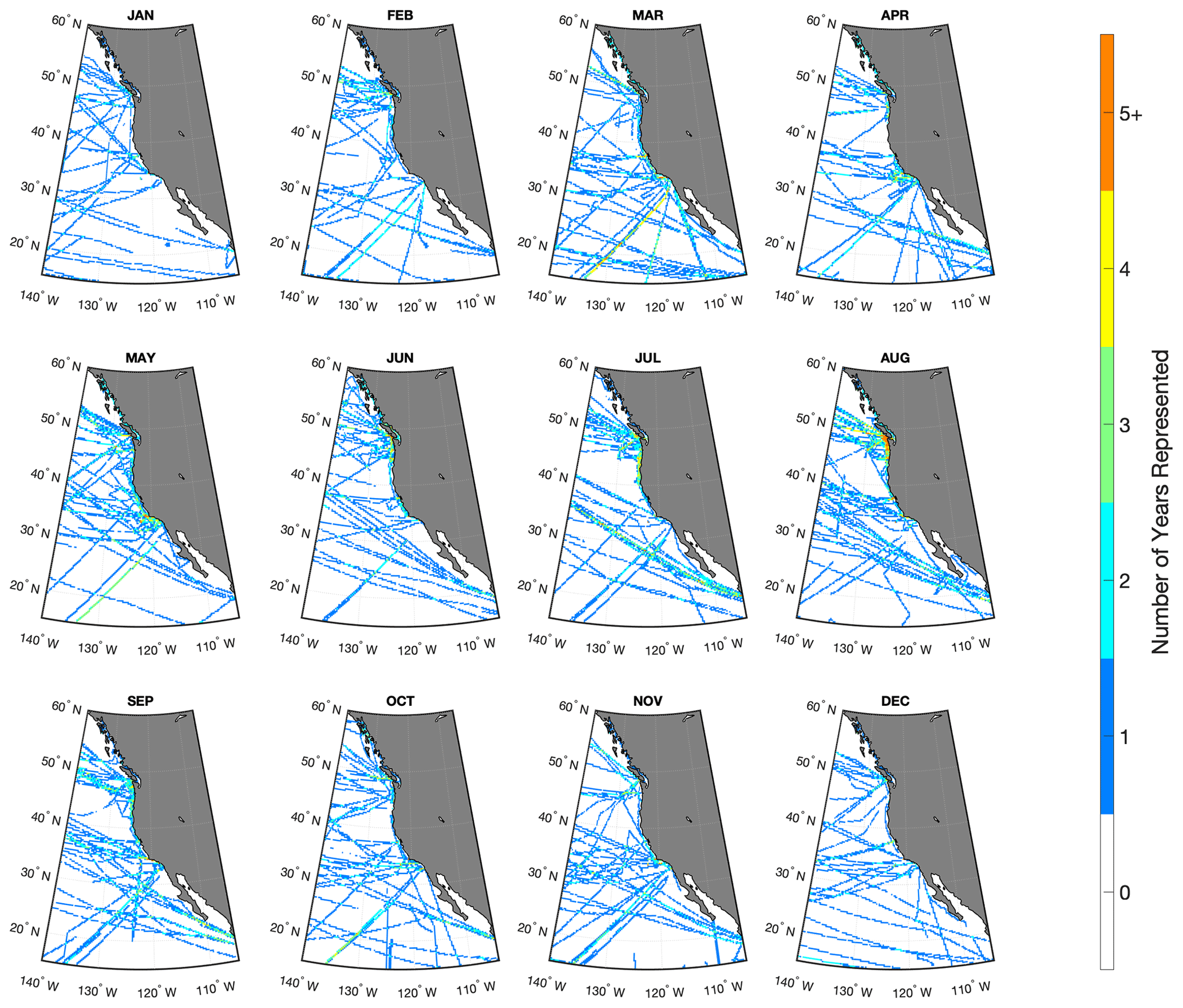
Figure B1The number of years containing a pCO2(sw) observation within each month over the 23 years of our gridded pCO2(sw) data product from 1998–2020.
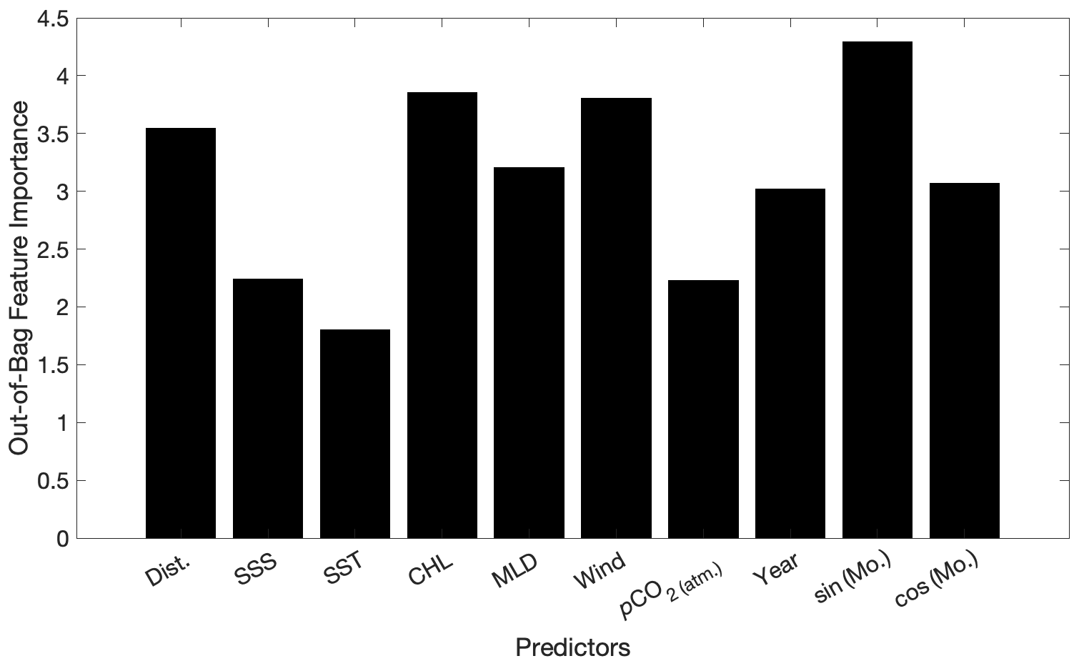
Figure B2Predictor variable feature importances calculated for the random forest regression model fit used to produce RFR-CCS (Sharp et al., 2022; https://doi.org/10.5281/zenodo.5523389).
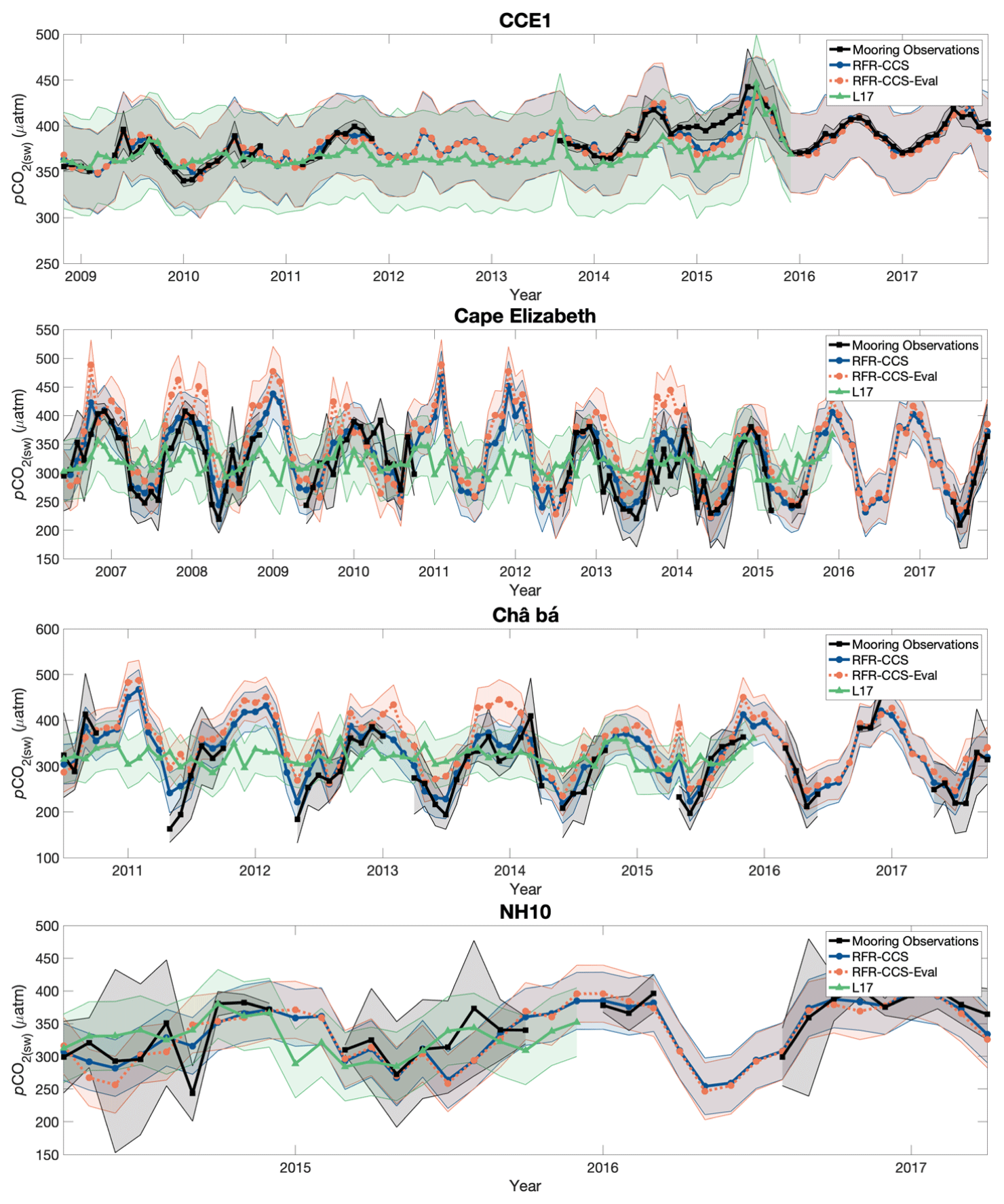
Figure B3Like Fig. 2 in the main text, showing monthly values of pCO2(sw) from mooring observations (black), RFR-CCS (blue), the mooring-excluded RFR-CCS-Eval model (orange), and L17 (green). The envelopes around the black lines equal the standard deviations of all mooring observations within each month, representing the natural variability of the 3-hourly mooring measurements; the envelopes around the blue and orange lines represent the RFR-CCS and RFR-CCS-Eval results plus 1 standard uncertainty (43.6 µatm; Sect. 3.5); the envelopes around the green lines represents the L17 data product plus the RMSE of an independent data evaluation in the province most closely associated with the mooring locations (52.5 µatm; Table 3 of Laruelle et al., 2017; Province P7).
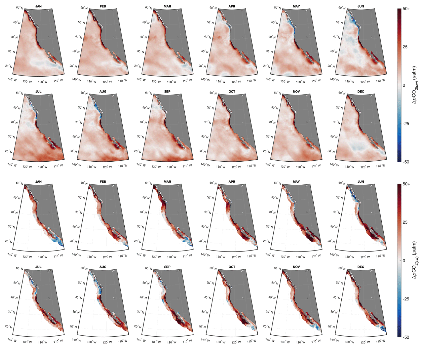
Figure B4Monthly mean differences in pCO2(sw) values between RFR-CCS-clim and L20 (top) and between RFR-CCS-clim and L17 (bottom).
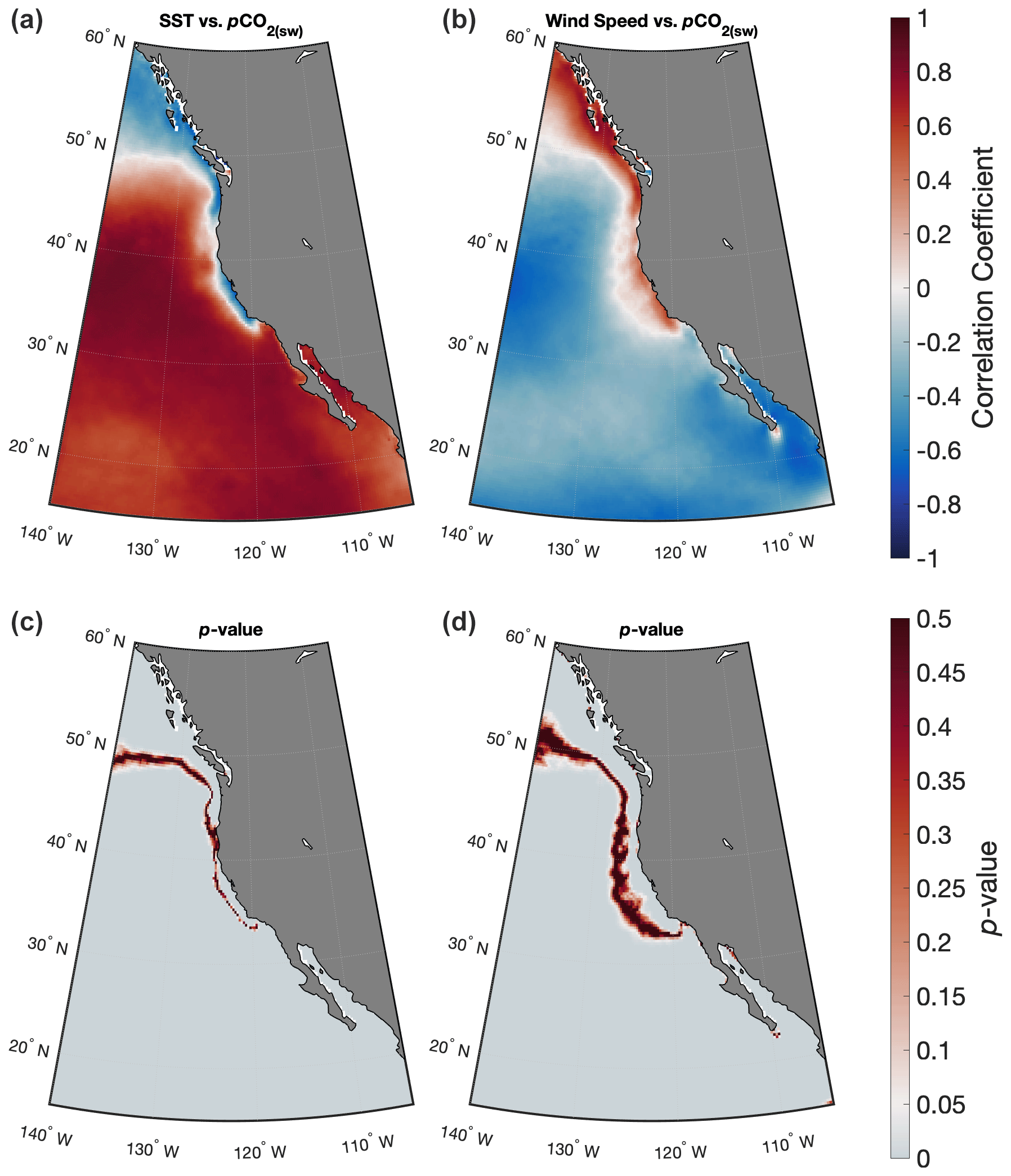
Figure B5Correlations (a, b) and the p values of those correlations (c, d) in each grid cell of RFR-CCS between pCO2(sw) and SST (a, c) and between pCO2(sw) and wind speed (b, d).
Table B1Mean biases (MBs), root mean squared errors (RMSEs), and coefficients of determination (R2) for comparisons of RFR-CCS, the mooring-excluded RFR-CCS-Eval, and L17 to mooring observations.
JDS, AJF, and BRC contributed to conceptualizing and planning the project. JDS conducted the analysis, produced the data visualizations, and wrote the original draft of the paper. JDS, AJF, BRC, PDL, and AJS reviewed and edited the paper.
The contact author has declared that neither they nor their co-authors have any competing interests.
Publisher's note: Copernicus Publications remains neutral with regard to jurisdictional claims in published maps and institutional affiliations.
The Surface Ocean CO2 Atlas (SOCAT) is an international effort endorsed by the International Ocean Carbon Coordination Project (IOCCP), the Surface Ocean Lower Atmosphere Study (SOLAS), and the Integrated Marine Biosphere Research (IMBeR) program to deliver a uniformly quality-controlled surface ocean CO2 database. The many researchers and funding agencies responsible for the collection of data and quality control are thanked for their contributions to SOCAT. The moored autonomous pCO2 observations are supported by the Global Ocean Monitoring and Observing (GOMO) Program and Ocean Acidification Program of the National Oceanic and Atmospheric Administration (NOAA). Jonathan D. Sharp and Andrea J. Fassbender were supported by the GOMO Program of NOAA. This is PMEL contribution no. 5290. Paige D. Lavin was supported by the Cooperative Institute for Climate, Ocean, & Ecosystem Studies (CISESS) at the University of Maryland/ESSIC. This publication is partially funded by the Cooperative Institute for Climate, Ocean, & Ecosystem Studies (CICOES), contribution no. 2021-1162.
This research has been supported by grant nos. NA20OAR4320271 (CICOES) and NA19NES4320002 (CISESS) from the National Oceanic and Atmospheric Administration.
This paper was edited by Anton Velo and reviewed by three anonymous referees.
Bakker, D. C. E., Pfeil, B., Landa, C. S., Metzl, N., O'Brien, K. M., Olsen, A., Smith, K., Cosca, C., Harasawa, S., Jones, S. D., Nakaoka, S., Nojiri, Y., Schuster, U., Steinhoff, T., Sweeney, C., Takahashi, T., Tilbrook, B., Wada, C., Wanninkhof, R., Alin, S. R., Balestrini, C. F., Barbero, L., Bates, N. R., Bianchi, A. A., Bonou, F., Boutin, J., Bozec, Y., Burger, E. F., Cai, W.-J., Castle, R. D., Chen, L., Chierici, M., Currie, K., Evans, W., Featherstone, C., Feely, R. A., Fransson, A., Goyet, C., Greenwood, N., Gregor, L., Hankin, S., Hardman-Mountford, N. J., Harlay, J., Hauck, J., Hoppema, M., Humphreys, M. P., Hunt, C. W., Huss, B., Ibánhez, J. S. P., Johannessen, T., Keeling, R., Kitidis, V., Körtzinger, A., Kozyr, A., Krasakopoulou, E., Kuwata, A., Landschützer, P., Lauvset, S. K., Lefèvre, N., Lo Monaco, C., Manke, A., Mathis, J. T., Merlivat, L., Millero, F. J., Monteiro, P. M. S., Munro, D. R., Murata, A., Newberger, T., Omar, A. M., Ono, T., Paterson, K., Pearce, D., Pierrot, D., Robbins, L. L., Saito, S., Salisbury, J., Schlitzer, R., Schneider, B., Schweitzer, R., Sieger, R., Skjelvan, I., Sullivan, K. F., Sutherland, S. C., Sutton, A. J., Tadokoro, K., Telszewski, M., Tuma, M., van Heuven, S. M. A. C., Vandemark, D., Ward, B., Watson, A. J., and Xu, S.: A multi-decade record of high-quality fCO2 data in version 3 of the Surface Ocean CO2 Atlas (SOCAT), Earth Syst. Sci. Data, 8, 383–413, https://doi.org/10.5194/essd-8-383-2016, 2016.
Becker, M., Olsen, A., Landschützer, P., Omar, A., Rehder, G., Rödenbeck, C., and Skjelvan, I.: The northern European shelf as an increasing net sink for CO2, Biogeosciences, 18, 1127–1147, https://doi.org/10.5194/bg-18-1127-2021, 2021.
Bourgeois, T., Orr, J. C., Resplandy, L., Terhaar, J., Ethé, C., Gehlen, M., and Bopp, L.: Coastal-ocean uptake of anthropogenic carbon, Biogeosciences, 13, 4167–4185, https://doi.org/10.5194/bg-13-4167-2016, 2016.
Breiman, L.: Bagging predictors, Mach. Learn. 24, 123–140, https://doi.org/10.1007/BF00058655, 1996.
Breiman, L.: Random forests, Mach. Learn., 45, 5–32, https://doi.org/10.1023/A:1010933404324, 2001.
Bushinsky, S. M., Landschützer, P., Rödenbeck, C., Gray, A. R., Baker, D., Mazloff, M. R., Resplandy, L., Johnson, K. S., and Sarmiento, J. L.: Reassessing Southern Ocean Air-Sea CO2 Flux Estimates With the Addition of Biogeochemical Float Observations, Global Biogeochem. Cy., 33, 1370–1388, https://doi.org/10.1029/2019GB006176, 2019.
Caldeira, K. and Wickett, M. E.: Anthropogenic carbon and ocean pH, Nature, 425, 365, https://doi.org/10.1038/425365a, 2003.
Chassignet, E. P., Hurlburt, H. E., Smedstad, O. M., Halliwell, G. R., Hogan, P. J., Wallcraft, A. J., Baraille, R., and Bleck, R.: The HYCOM (hybrid coordinate ocean model) data assimilative system, J. Mar. Syst., 65, 60–83, https://doi.org/10.1016/j.jmarsys.2005.09.016, 2007.
Chau, T. T. T., Gehlen, M., and Chevallier, F.: A seamless ensemble-based reconstruction of surface ocean pCO2 and air–sea CO2 fluxes over the global coastal and open oceans, Biogeosciences, 19, 1087–1109, https://doi.org/10.5194/bg-19-1087-2022, 2022.
Checkley, D. M. and Barth, J. A.: Patterns and processes in the California Current System, Prog. Oceanogr., 83, 49–64, https://doi.org/10.1016/j.pocean.2009.07.028, 2009.
Chen, S., Hu, C., Barnes, B. B., Wanninkhof, R., Cai, W. J., Barbero, L., and Pierrot, D.: A machine learning approach to estimate surface ocean pCO2 from satellite measurements, Remote Sens. Environ., 228, 203–226, https://doi.org/10.1016/j.rse.2019.04.019, 2019.
Ciais, P., Sabine, C., Bala, G., Bopp, L., Brovkin, V., Canadell, J., Chhabra, A., DeFries, R., Galloway, J., Heimann, M., and Jones, C.: Carbon and other biogeochemical cycles, in: Climate change 2013: the physical science basis, Contribution of Working Group I to the Fifth Assessment Report of the Intergovernmental Panel on Climate Change, 465–570, Cambridge University Press, 465–570, https://doi.org/10.1017/CBO9781107415324.015, 2014.
Dai, M.: What are the exchanges of carbon between the land-ocean-ice continuum, in: Integrated Ocean Carbon Research: A Summary of Ocean Carbon Research, and Vision of Coordinated Ocean Carbon Research and Observations for the Next Decade, edited by: Wanninkhof, R., Sabine, C., and Aricò, S., IOC Technical Series, 158, Paris, UNESCO, 20, https://doi.org/10.25607/h0gj-pq41, 2021.
Denvil-Sommer, A., Gehlen, M., Vrac, M., and Mejia, C.: LSCE-FFNN-v1: a two-step neural network model for the reconstruction of surface ocean pCO2 over the global ocean, Geosci. Model Dev., 12, 2091–2105, https://doi.org/10.5194/gmd-12-2091-2019, 2019.
Deutsch, C., Frenzel, H., McWilliams, J. C., Renault, L., Kessouri, F., Howard, E., Liang, J. H., Bianchi, D., and Yang, S.: Biogeochemical variability in the California Current system, Prog. Oceanogr., 102565, https://doi.org/10.1016/j.pocean.2021.102565, 2021.
DeVries, T., Le Quéré, C., Andrews, O., Berthet, S., Hauck, J., Ilyina, T., Landschützer, P., Lenton, A., Lima, I. D., Nowicki, M., Schwinger, J., and Séférian, R. Decadal trends in the ocean carbon sink, P. Natl. Acad. Sci. USA, 116, 11646–1165, https://doi.org/10.1073/pnas.1900371116, 2019.
Dickson, A. G., Sabine, C. L., and Christian, J. R. (Eds.): Guide to Best Practices for Ocean CO2 Measurements. North Pacific Marine Science Organization, PICES Special Publication 3, Sidney, B.C., Canada, 2007.
Djeutchouang, L. M., Chang, N., Gregor, L., Vichi, M., and Monteiro, P. M. S.: The sensitivity of pCO2 reconstructions in the Southern Ocean to sampling scales: a semi-idealized model sampling and reconstruction approach, Biogeosciences Discuss. [preprint], https://doi.org/10.5194/bg-2021-344, in review, 2022.
Dlugokencky, E. and Tans, P.: Trends in atmospheric carbon dioxide, National Oceanic & Atmospheric Administration, Earth System Research Laboratory (NOAA/ESRL), http://www.esrl.noaa.gov/gmd/ccgg/trends/global.html (last access: 17 August 2021), 2019.
Dlugokencky, E. J., Mund, J. W., Crotwell, A. M., Crotwell, M. J., and Thoning, K. W.: Atmospheric carbon dioxide dry air mole fractions from the NOAA ESRL carbon cycle cooperative global air sampling network, 1968–2018, Version: 2019–2007, https://doi.org/10.15138/wkgj-f215, 2020.
Doney, S. C., Fabry, V. J., Feely, R. A., and Kleypas, J. A.: Ocean Acidification: The other CO2 problem, Annu. Rev. Mar. Sci., 1, 169–192, https://doi.org/10.1146/annurev.marine.010908.163834, 2009.
Doney, S. C., Busch, D. S., Cooley, S. R., and Kroeker, K. J.: The impacts of ocean acidification on marine ecosystems and reliant human communities, Annu. Rev. Environ. Res., 45, 83–112, https://doi.org/10.1146/annurev-environ-012320-083019, 2020.
Donlon, C. J., Minnett, P. J., Gentemann, C., Nightingale, T. J., Barton, I. J., Ward, B., and Murray, M. J.: Toward improved validation of satellite sea surface skin temperature measurements for climate research, J. Climate, 15, 353–369, https://doi.org/10.1175/1520-0442(2002)015<0353:TIVOSS>2.0.CO;2, 2002.
Evans, W., Hales, B., and Strutton, P. G.: Seasonal cycle of surface ocean pCO2 on the Oregon shelf, J. Geophys. Res.-Oceans, 116, C05012, https://doi.org/10.1029/2010JC006625, 2011.
Evans, W., Hales, B., Strutton, P. G., and Ianson, D. Sea-air CO2 fluxes in the western Canadian coastal ocean, Prog. Oceanogr., 101, 78–91, https://doi.org/10.1016/j.pocean.2012.01.003, 2012.
Evans, W., Lebon, G. T., Harrington, C. D., Takeshita, Y., and Bidlack, A.: Marine CO2 system variability along the northeast Pacific Inside Passage determined from an Alaskan ferry, Biogeosciences, 19, 1277–1301, https://doi.org/10.5194/bg-19-1277-2022, 2022.
Fabry, V. J., Seibel, B. A., Feely, R. A., and Orr, J. C.: Impacts of ocean acidification on marine fauna and ecosystem processes, ICES J. Mar. Sci., 65, 414–432, https://doi.org/10.1093/icesjms/fsn048, 2008.
Fassbender, A. J., Sabine, C. L., Feely, R. A., Langdon, C., and Mordy, C. W.: Inorganic carbon dynamics during northern California coastal upwelling, Cont. Shelf Res., 31, 1180–1192, https://doi.org/10.1016/j.csr.2011.04.006, 2011.
Fassbender, A. J., Alin, S. R., Feely, R. A., Sutton, A. J., Newton, J. A., Krembs, C., Bos, J., Keyzers, M., Devol, A., Ruef, W., and Pelletier, G.: Seasonal carbonate chemistry variability in marine surface waters of the US Pacific Northwest, Earth Syst. Sci. Data, 10, 1367–1401, https://doi.org/10.5194/essd-10-1367-2018, 2018.
Fay, A. R., Gregor, L., Landschützer, P., McKinley, G. A., Gruber, N., Gehlen, M., Iida, Y., Laruelle, G. G., Rödenbeck, C., Roobaert, A., and Zeng, J.: SeaFlux: harmonization of air–sea CO2 fluxes from surface pCO2 data products using a standardized approach, Earth Syst. Sci. Data, 13, 4693–4710, https://doi.org/10.5194/essd-13-4693-2021, 2021.
Feely, R. A., Sabine, C. L., Hernandez-Ayon, J. M., Ianson, D., and Hales, B.: Evidence for upwelling of corrosive “acidified” water onto the continental shelf, Science, 320, 1490–1492, https://doi.org/10.1126/science.1155676, 2008.
Fiechter, J., Curchitser, E. N., Edwards, C. A., Chai, F., Goebel, N. L., and Chavez, F. P.: Air-sea CO2 fluxes in the California Current: Impacts of model resolution and coastal topography, Global Biogeochem. Cy., 28, 371–385, https://doi.org/10.1002/2013GB004683, 2014.
Friedlingstein, P., O'Sullivan, M., Jones, M. W., Andrew, R. M., Hauck, J., Olsen, A., Peters, G. P., Peters, W., Pongratz, J., Sitch, S., Le Quéré, C., Canadell, J. G., Ciais, P., Jackson, R. B., Alin, S., Aragão, L. E. O. C., Arneth, A., Arora, V., Bates, N. R., Becker, M., Benoit-Cattin, A., Bittig, H. C., Bopp, L., Bultan, S., Chandra, N., Chevallier, F., Chini, L. P., Evans, W., Florentie, L., Forster, P. M., Gasser, T., Gehlen, M., Gilfillan, D., Gkritzalis, T., Gregor, L., Gruber, N., Harris, I., Hartung, K., Haverd, V., Houghton, R. A., Ilyina, T., Jain, A. K., Joetzjer, E., Kadono, K., Kato, E., Kitidis, V., Korsbakken, J. I., Landschützer, P., Lefèvre, N., Lenton, A., Lienert, S., Liu, Z., Lombardozzi, D., Marland, G., Metzl, N., Munro, D. R., Nabel, J. E. M. S., Nakaoka, S.-I., Niwa, Y., O'Brien, K., Ono, T., Palmer, P. I., Pierrot, D., Poulter, B., Resplandy, L., Robertson, E., Rödenbeck, C., Schwinger, J., Séférian, R., Skjelvan, I., Smith, A. J. P., Sutton, A. J., Tanhua, T., Tans, P. P., Tian, H., Tilbrook, B., van der Werf, G., Vuichard, N., Walker, A. P., Wanninkhof, R., Watson, A. J., Willis, D., Wiltshire, A. J., Yuan, W., Yue, X., and Zaehle, S.: Global Carbon Budget 2020, Earth Syst. Sci. Data, 12, 3269–3340, https://doi.org/10.5194/essd-12-3269-2020, 2020.
Friederich, G. M., Walz, P. M., Burczynski, M. G., and Chavez, F. P.: Inorganic carbon in the central California upwelling system during the 1997–1999 El Niño–La Niña event, Prog. Oceanogr., 54, 185–203, https://doi.org/10.1016/S0079-6611(02)00049-6, 2002.
Gloege, L., McKinley, G. A., Landschützer, P., Fay, A. R., Frölicher, T. L., Fyfe, J. C., Ilyina, T., Jones, S., Lovenduski, N. S., Rodgers, K. B., Schlunegger, S., and Takano, Y.: Quantifying errors in observationally based estimates of ocean carbon sink variability, Global Biogeochem. Cy., 35, e2020GB006788, https://doi.org/10.1029/2020GB006788, 2021.
Goddijn-Murphy, L. M., Woolf, D. K., Land, P. E., Shutler, J. D., and Donlon, C.: The OceanFlux Greenhouse Gases methodology for deriving a sea surface climatology of CO2 fugacity in support of air–sea gas flux studies, Ocean Sci., 11, 519–541, https://doi.org/10.5194/os-11-519-2015, 2015.
Greene, C. A., Thirumalai, K., Kearney, K. A., Delgado, J. M., Schwanghart, W., Wolfenbarger, N. S., Thyng, K. M., Gwyther, D. E., Gardner, A. S., and Blankenship, D. D.: The Climate Data Toolbox for MATLAB, Geochem. Geophy. Geosy., 20, 3774–3781, https://doi.org/10.1029/2019GC008392, 2019.
Gregor, L. and Fay, A.: SeaFlux: harmonised sea-air CO2 fluxes from surface pCO2 data products using a standardised approach (2021.04.03), Zenodo [data set], https://doi.org/10.5281/zenodo.5148795, 2021.
Gregor, L., Kok, S., and Monteiro, P. M. S.: Empirical methods for the estimation of Southern Ocean CO2: support vector and random forest regression, Biogeosciences, 14, 5551–5569, https://doi.org/10.5194/bg-14-5551-2017, 2017.
Gregor, L., Kok, S., and Monteiro, P. M. S.: Interannual drivers of the seasonal cycle of CO2 in the Southern Ocean, Biogeosciences, 15, 2361–2378, https://doi.org/10.5194/bg-15-2361-2018, 2018.
Gregor, L., Lebehot, A. D., Kok, S., and Scheel Monteiro, P. M.: A comparative assessment of the uncertainties of global surface ocean CO2 estimates using a machine-learning ensemble (CSIR-ML6 version 2019a) – have we hit the wall?, Geosci. Model Dev., 12, 5113–5136, https://doi.org/10.5194/gmd-12-5113-2019, 2019.
Gruber, N., Hauri, C., Lachkar, Z., Loher, D., Frolicher, T. L., and Plattner, G.-K.: Rapid Progression of Ocean Acidification in the California Current System, Science, 337, 220–223, https://doi.org/10.1126/science.1216773, 2012.
Hales, B., Takahashi, T., and Bandstra, L.: Atmospheric CO2 uptake by a coastal upwelling system, Global Biogeochem. Cy., 19, 1–11, https://doi.org/10.1029/2004GB002295, 2005.
Hales, B., Strutton, P. G., Saraceno, M., Letelier, R., Takahashi, T., Feely, R., Sabine, C., and Chavez, F.: Satellite-based prediction of pCO2 in coastal waters of the eastern North Pacific, Prog. Oceanogr., 103, 1–15, https://doi.org/10.1016/j.pocean.2012.03.001, 2012.
Hastie, T., Tibshirani, R., and Friedman, J. H.: The elements of statistical learning: data mining, inference, and prediction, 2nd Edn., Springer, New York, NY, https://doi.org/10.1007/978-0-387-84858-7, 2009.
Hauck, J., Zeising, M., Le Quéré, C., Gruber, N., Bakker, D. C. E., Bopp, L., Chau, T. T. T., Gürses, Ö., Ilyina, T., Landschützer, P., Lenton, A., Resplandy, L., Rödenbeck, C., Schwinger, J., and Séférian, R.: Consistency and Challenges in the Ocean Carbon Sink Estimate for the Global Carbon Budget, Front. Mar. Sci., 7, 1–22, https://doi.org/10.3389/fmars.2020.571720, 2020.
Hauri, C., Gruber, N., Vogt, M., Doney, S. C., Feely, R. A., Lachkar, Z., Leinweber, A., McDonnell, A. M. P., Munnich, M., and Plattner, G.-K.: Spatiotemporal variability and long-term trends of ocean acidification in the California Current System, Biogeosciences, 10, 193–216, https://doi.org/10.5194/bg-10-193-2013, 2013.
Hersbach, H., Bell, B., Berrisford, P., Hirahara, S., Horányi, A., Muñoz-Sabater, J., Nicolas, J., Peubey, C., Radu, R., Schepers, D., Simmons, A., Soci, C., Abdalla, S., Abellan, X., Balsamo, G., Bechtold, P., Biavati, G., Bidlot, J., Bonavita, M., De Chiara, G., Dahlgren, P., Dee, D., Diamantakis, M., Dragani, R., Flemming, J., Forbes, R., Fuentes, M., Geer, A., Haimberger, L., Healy, S., Hogan, R. J., Hólm, E., Janisková, M., Keeley, S., Laloyaux, P., Lopez, P., Lupu, C., Radnoti, G., de Rosnay, P., Rozum, I., Vamborg, F., Villaume, S., and Thépaut, J. N.: The ERA5 global reanalysis, Q. J. Roy. Meteor. Soc., 146, 1999–2049, https://doi.org/10.1002/qj.3803, 2020.
Hickey, B. M. and Banas, N. S.: Why is the northern end of the California Current System so productive?, Oceanography, 21, 90–107, https://doi.org/10.5670/oceanog.2008.07, 2008.
Ho, D. T. and Schanze, J. J. Precipitation-Induced Reduction in Surface Ocean pCO2: Observations From the Eastern Tropical Pacific Ocean, Geophys. Res. Lett., 47, e2020GL088252, https://doi.org/10.1029/2020GL088252, 2020.
Huang, B., Liu, C., Banzon, V., Freeman, E., Graham, G., Hankins, B., Smith, T., and Zhang, H.-M.: Improvements of the Daily Optimum Interpolation Sea Surface Temperature (DOISST) Version 2.1, J. Climate, 34, 2923–2939, https://doi.org/10.1175/JCLI-D-20-0166.1, 2021.
Huyer, A.: Coastal upwelling in the California Current system, Prog. Oceanogr., 12, 259–284, https://doi.org/10.1016/0079-6611(83)90010-1, 1983.
Ianson, D., Allen, S. E., Harris, S. L., Orians, K. J., Varela, D. E., and Wong, C. S.: The inorganic carbon system in the coastal upwelling region west of Vancouver Island, Canada, Deep-Sea Res. Pt. I, 50, 1023–1042, https://doi.org/10.1016/S0967-0637(03)00114-6, 2003.
Iida, Y., Kojima, A., Takatani, Y., Nakano, T., Sugimoto, H., Midorikawa, T., and Ishii, M.: Trends in pCO2 and sea–air CO2 flux over the global open oceans for the last two decades, J. Oceanogr., 71, 637–661, https://doi.org/10.1007/s10872-015-0306-4, 2015.
Ishii, M., Feely, R. A., Rodgers, K. B., Park, G.-H., Wanninkhof, R., Sasano, D., Sugimoto, H., Cosca, C. E., Nakaoka, S., Telszewski, M., Nojiri, Y., Mikaloff Fletcher, S. E., Niwa, Y., Patra, P. K., Valsala, V., Nakano, H., Lima, I., Doney, S. C., Buitenhuis, E. T., Aumont, O., Dunne, J. P., Lenton, A., and Takahashi, T.: Air–sea CO2 flux in the Pacific Ocean for the period 1990–2009, Biogeosciences, 11, 709–734, https://doi.org/10.5194/bg-11-709-2014, 2014.
Jones, S. D., Le Quéré, C., Rödenbeck, C., Manning, A. C., and Olsen, A.: A statistical gap-filling method to interpolate global monthly surface ocean carbon dioxide data, J. Adv. Model. Earth Sy., 7, 1554–1575, https://doi.org/10.1002/2014MS000416, 2015.
Joos, F. and Spahni, R. Rates of change in natural and anthropogenic radiative forcing over the past 20,000 years, P. Natl. Acad. Sci. USA, 105, 1425–1430, https://doi.org/10.1073/pnas.0707386105, 2008.
Landschützer, P., Gruber, N., Bakker, D. C. E., Schuster, U., Nakaoka, S., Payne, M. R., Sasse, T. P., and Zeng, J.: A neural network-based estimate of the seasonal to inter-annual variability of the Atlantic Ocean carbon sink, Biogeosciences, 10, 7793–7815, https://doi.org/10.5194/bg-10-7793-2013, 2013.
Landschützer, P., Gruber, N., Bakker, D. C. E., and Schuster, U.: Recent variability of the global ocean carbon sink, Global Biogeochem. Cy., 28, 927–949, https://doi.org/10.1002/2014GB004853, 2014.
Landschützer, P., Gruber, N., Haumann, F. A., Rödenbeck, C., Bakker, D. C. E., van Heuven, S., Hoppema, M., Metzl, N., Sweeney, C., Takahashi, T., Tilbrook, B., and Wanninkhof, R.: The reinvigoration of the Southern Ocean carbon sink, Science, 349, 1221–1224, https://doi.org/10.1126/science.aab2620, 2015.
Landschützer, P., Gruber, N., and Bakker, D. C. E.: Decadal variations and trends of the global ocean carbon sink, Global Biogeochem. Cy., 30, 1396–1417, https://doi.org/10.1002/2015GB005359, 2016.
Landschützer, P., Gruber, N., Bakker, D. C. E., Stemmler, I., and Six, K. D.: Strengthening seasonal marine CO2 variations due to increasing atmospheric CO2, Nat. Clim. Change, 8, 146–150, https://doi.org/10.1038/s41558-017-0057-x, 2018.
Landschützer, P., Gruber, N., and Bakker, D. C. E.: An observation-based global monthly gridded sea surface pCO2 product from 1982 onward and its monthly climatology (NCEI Accession 0160558), Version 5.5, NOAA National Centers for Environmental Information [data set], https://doi.org/10.7289/V5Z899N6, 2020a.
Landschützer, P., Laruelle, G., Roobaert, A., Regnier, P.: A combined global ocean pCO2 climatology combining open ocean and coastal areas (NCEI Accession 0209633), NOAA National Centers for Environmental Information [data set], https://doi.org/10.25921/qb25-f418, 2020b.
Landschützer, P., Laruelle, G. G., Roobaert, A., and Regnier, P.: A uniform pCO2 climatology combining open and coastal oceans, Earth Syst. Sci. Data, 12, 2537–2553, https://doi.org/10.5194/essd-12-2537-2020, 2020c.
Laruelle, G. G., Dürr, H. H., Slomp, C. P., and Borges, A. V.: Evaluation of sinks and sources of CO2 in the global coastal ocean using a spatially-explicit typology of estuaries and continental shelves. Geophys. Res. Lett., 37, L15607, https://doi.org/10.1029/2010GL043691, 2010.
Laruelle, G. G., Lauerwald, R., Pfeil, B., and Regnier, P.: Regionalized global budget of the CO2 exchange at the air-water interface in continental shelf seas, Global Biogeochem. Cy., 28, 1199–1214, https://doi.org/10.1111/1462-2920.13280, 2014.
Laruelle, G. G., Landschützer, P., Gruber, N., Tison, J.-L., Delille, B., and Regnier, P.: Global high-resolution monthly pCO2 climatology for the coastal ocean derived from neural network interpolation, Biogeosciences, 14, 4545–4561, https://doi.org/10.5194/bg-14-4545-2017, 2017.
Laruelle, G. G., Cai, W. J., Hu, X., Gruber, N., Mackenzie, F. T., and Regnier, P.: Continental shelves as a variable but increasing global sink for atmospheric carbon dioxide, Nat. Commun., 9, 1–11, https://doi.org/10.1038/s41467-017-02738-z, 2018.
Lauvset, S., Currie, K., Metzl, N., Nakaoka, S. I., Bakker, D., Sullivan, K., Sutton, A., O'Brien, K., and Olsen, A.: SOCAT Quality Control Cookbook: for SOCAT version 7, SOCAT, https://doi.org/10.25607/OBP-1665, 2018.
Lebehot, A. D., Halloran, P. R., Watson, A. J., McNeall, D., Ford, D. A., Landschützer, P., Lauvset, S. K., and Schuster, U.: Reconciling Observation and Model Trends in North Atlantic Surface CO2, Global Biogeochem. Cy., 33, 1204–1222 https://doi.org/10.1029/2019GB006186, 2019.
Majkut, J. D., Sarmiento, J. L., and Rodgers, K. B.: A growing oceanic carbon uptake: Results from an inversion study of surface pCO2 data, Global Biochem. Cy., 28, 335–351, https://doi.org/10.1002/2013GB004585, 2014.
Meinig, C., Burger, E. F., Cohen, N., Cokelet, E. D., Cronin, M. F., Cross, J. N., de Halleux, S., Jenkins, R., Jessup, A. T., Mordy, C. W., Lawrence-Slavas, N., Sutton, A. J., Zhang, D., and Zhang, C.: Public–private partnerships to advance regional ocean-observing capabilities: a saildrone and NOAA-PMEL case study and future considerations to expand to global scale observing, Front. Mar. Sci., 13, 448, https://doi.org/10.3389/fmars.2019.00448, 2015.
Menemenlis, D., Fukumori, I., and Lee, T.: Using Green's functions to calibrate an ocean general circulation model, Mon. Weather Rev., 133, 1224–1240, https://doi.org/10.1175/MWR2912.1, 2005.
Menemenlis, D., Campin, J. M., Heimbach, P., Hill, C., Lee, T., Nguyen, A., Schodlok, M., and Zhang, H.: ECCO2: High resolution global ocean and sea ice data synthesis, Mercator Ocean Quarterly Newsletter, 31, 13–21, 2008.
Monteiro, P. M. S., Gregor, L., Lévy, M., Maenner, S., Sabine, C. L., and Swart, S.: Intraseasonal variability linked to sampling alias in air-sea CO2 fluxes in the Southern Ocean, Geophys. Res. Lett., 42, 8507–8514, https://doi.org/10.1002/2015GL066009, 2015.
Nakaoka, S., Telszewski, M., Nojiri, Y., Yasunaka, S., Miyazaki, C., Mukai, H., and Usui, N.: Estimating temporal and spatial variation of ocean surface pCO2 in the North Pacific using a self-organizing map neural network technique, Biogeosciences, 10, 6093–6106, https://doi.org/10.5194/bg-10-6093-2013, 2013.
Orr, J. C., Fabry, V. J., Aumont, O., Bopp, L., Doney, S. C., Feely, R. A., Gnanadesikan, A., Gruber, N., Ishida, A., Joos, F., Key, R. M., Lindsay, K., Maier-Reimer, E., Matear, R., Monfray, P., Mouchet, A., Najjar, R. G., Plattner, G. K., Rodgers, K. B., Sabine, C. L., Sarmiento, J. L., Schlitzer, R., Slater, R. D., Totterdell, I. J., Weirig, M.-F., Yamanaka, Y., and Yool, A.: Anthropogenic ocean acidification over the twenty-first century and its impact on calcifying organisms, Nature, 437, 681–686, https://doi.org/10.1038/nature04095, 2005.
Pfeil, B., Olsen, A., Bakker, D. C. E., Hankin, S., Koyuk, H., Kozyr, A., Malczyk, J., Manke, A., Metzl, N., Sabine, C. L., Akl, J., Alin, S. R., Bates, N., Bellerby, R. G. J., Borges, A., Boutin, J., Brown, P. J., Cai, W.-J., Chavez, F. P., Chen, A., Cosca, C., Fassbender, A. J., Feely, R. A., González-Dávila, M., Goyet, C., Hales, B., Hardman-Mountford, N., Heinze, C., Hood, M., Hoppema, M., Hunt, C. W., Hydes, D., Ishii, M., Johannessen, T., Jones, S. D., Key, R. M., Körtzinger, A., Landschützer, P., Lauvset, S. K., Lefèvre, N., Lenton, A., Lourantou, A., Merlivat, L., Midorikawa, T., Mintrop, L., Miyazaki, C., Murata, A., Nakadate, A., Nakano, Y., Nakaoka, S., Nojiri, Y., Omar, A. M., Padin, X. A., Park, G.-H., Paterson, K., Perez, F. F., Pierrot, D., Poisson, A., Ríos, A. F., Santana-Casiano, J. M., Salisbury, J., Sarma, V. V. S. S., Schlitzer, R., Schneider, B., Schuster, U., Sieger, R., Skjelvan, I., Steinhoff, T., Suzuki, T., Takahashi, T., Tedesco, K., Telszewski, M., Thomas, H., Tilbrook, B., Tjiputra, J., Vandemark, D., Veness, T., Wanninkhof, R., Watson, A. J., Weiss, R., Wong, C. S., and Yoshikawa-Inoue, H.: A uniform, quality controlled Surface Ocean CO2 Atlas (SOCAT), Earth Syst. Sci. Data, 5, 125–143, https://doi.org/10.5194/essd-5-125-2013, 2013.
Pierrot, D., Neill, C., Sullivan, K., Castle, R., Wanninkhof, R., Lüger, H., Johannessen, T., Olsen, A., Feely, R. A., and Cosca, C. E.: Recommendations for autonomous underway pCO2 measuring systems and data-reduction routines, Deep-Sea Res. II, 56, 512–522, https://doi.org/10.1016/j.dsr2.2008.12.005, 2009.
Pörtner, H. O.: Ecosystem effects of ocean acidification in times of ocean warming: a physiologist's view, Mar. Ecol. Prog. Ser., 373, 203–217, https://doi.org/10.3354/meps07768, 2008.
Reynolds, R. W., Smith, T. M., Liu, C., Chelton, D. B., Casey, K. S., and Schlax, M. G.: Daily high-resolution-blended analyses for sea surface temperature, J. Climate, 20, 5473–5496, https://doi.org/10.1175/2007JCLI1824.1, 2007.
Ritter, R., Landschützer, P., Gruber, N., Fay, A. R., Iida, Y., Jones, S., and Zeng, J.: Observation-Based Trends of the Southern Ocean Carbon Sink, Geophys. Res. Lett., 2, 339–348, https://doi.org/10.1002/2017GL074837, 2017.
Robertson, J. E. and Watson, A. J.: Thermal skin effect of the surface ocean and its implications for CO2 uptake, Nature, 358, 738–740, https://doi.org/10.1038/358738a0, 1992.
Rödenbeck, C., Keeling, R. F., Bakker, D. C. E., Metzl, N., Olsen, A., Sabine, C., and Heimann, M.: Global surface-ocean pCO2 and sea–air CO2 flux variability from an observation-driven ocean mixed-layer scheme, Ocean Sci., 9, 193–216, https://doi.org/10.5194/os-9-193-2013, 2013.
Rödenbeck, C., Bakker, D. C. E., Metzl, N., Olsen, A., Sabine, C., Cassar, N., Reum, F., Keeling, R. F., and Heimann, M.: Interannual sea–air CO2 flux variability from an observation-driven ocean mixed-layer scheme, Biogeosciences, 11, 4599–4613, https://doi.org/10.5194/bg-11-4599-2014, 2014.
Rödenbeck, C., Bakker, D. C. E., Gruber, N., Iida, Y., Jacobson, A. R., Jones, S., Landschützer, P., Metzl, N., Nakaoka, S., Olsen, A., Park, G.-H., Peylin, P., Rodgers, K. B., Sasse, T. P., Schuster, U., Shutler, J. D., Valsala, V., Wanninkhof, R., and Zeng, J.: Data-based estimates of the ocean carbon sink variability – first results of the Surface Ocean pCO2 Mapping intercomparison (SOCOM), Biogeosciences, 12, 7251–7278, https://doi.org/10.5194/bg-12-7251-2015, 2015.
Roobaert, A., Laruelle, G. G., Landschützer, P., Gruber, N., Chou, L., and Regnier, P. The Spatiotemporal Dynamics of the Sources and Sinks of CO2 in the Global Coastal Ocean, Global Biogeochem. Cy., 33, 1693–1714, https://doi.org/10.1029/2019GB006239, 2019.
Sabine, C. L., Hankin, S., Koyuk, H., Bakker, D. C. E., Pfeil, B., Olsen, A., Metzl, N., Kozyr, A., Fassbender, A., Manke, A., Malczyk, J., Akl, J., Alin, S. R., Bellerby, R. G. J., Borges, A., Boutin, J., Brown, P. J., Cai, W.-J., Chavez, F. P., Chen, A., Cosca, C., Feely, R. A., González-Dávila, M., Goyet, C., Hardman-Mountford, N., Heinze, C., Hoppema, M., Hunt, C. W., Hydes, D., Ishii, M., Johannessen, T., Key, R. M., Körtzinger, A., Landschützer, P., Lauvset, S. K., Lefèvre, N., Lenton, A., Lourantou, A., Merlivat, L., Midorikawa, T., Mintrop, L., Miyazaki, C., Murata, A., Nakadate, A., Nakano, Y., Nakaoka, S., Nojiri, Y., Omar, A. M., Padin, X. A., Park, G.-H., Paterson, K., Perez, F. F., Pierrot, D., Poisson, A., Ríos, A. F., Salisbury, J., Santana-Casiano, J. M., Sarma, V. V. S. S., Schlitzer, R., Schneider, B., Schuster, U., Sieger, R., Skjelvan, I., Steinhoff, T., Suzuki, T., Takahashi, T., Tedesco, K., Telszewski, M., Thomas, H., Tilbrook, B., Vandemark, D., Veness, T., Watson, A. J., Weiss, R., Wong, C. S., and Yoshikawa-Inoue, H.: Surface Ocean CO2 Atlas (SOCAT) gridded data products, Earth Syst. Sci. Data, 5, 145–153, https://doi.org/10.5194/essd-5-145-2013, 2013.
Schuster, U., McKinley, G. A., Bates, N., Chevallier, F., Doney, S. C., Fay, A. R., González-Dávila, M., Gruber, N., Jones, S., Krijnen, J., Landschützer, P., Lefèvre, N., Manizza, M., Mathis, J., Metzl, N., Olsen, A., Rios, A. F., Rödenbeck, C., Santana-Casiano, J. M., Takahashi, T., Wanninkhof, R., and Watson, A. J.: An assessment of the Atlantic and Arctic sea–air CO2 fluxes, 1990–2009, Biogeosciences, 10, 607–627, https://doi.org/10.5194/bg-10-607-2013, 2013.
Sharp, J. D.: RFR-CCS Code (v1.0), Zenodo [code], https://doi.org/10.5281/zenodo.6484875, 2022.
Sharp, J. D., Fassbender, A. J., Carter, B. R., Lavin, P. D., and Sutton, A. J.: RFR-CCS: A monthly surface pCO2 product for the California Current Large Marine Ecosystem (v1.1), Zenodo [data set], https://doi.org/10.5281/zenodo.5523389, 2022.
Shutler, J. D., Land, P. E., Piolle, J. F., Woolf, D. K., Goddijn-Murphy, L., Paul, F., Girard-Ardhuin, F., Chapron, B., and Donlon, C. J.: FluxEngine: a flexible processing system for calculating atmosphere–ocean carbon dioxide gas fluxes and climatologies, J. Atmos. Ocean. Tech., 33, 741–756, https://doi.org/10.1175/JTECH-D-14-00204.1, 2016.
Sutton, A. J., Feely, R. A., Maenner-Jones, S., Musielwicz, S., Osborne, J., Dietrich, C., Monacci, N., Cross, J., Bott, R., Kozyr, A., Andersson, A. J., Bates, N. R., Cai, W.-J., Cronin, M. F., De Carlo, E. H., Hales, B., Howden, S. D., Lee, C. M., Manzello, D. P., McPhaden, M. J., Meléndez, M., Mickett, J. B., Newton, J. A., Noakes, S. E., Noh, J. H., Olafsdottir, S. R., Salisbury, J. E., Send, U., Trull, T. W., Vandemark, D. C., and Weller, R. A.: Autonomous seawater pCO2 and pH time series from 40 surface buoys and the emergence of anthropogenic trends, Earth Syst. Sci. Data, 11, 421–439, https://doi.org/10.5194/essd-11-421-2019, 2019.
Sutton, A. J., Williams, N. L., and Tilbrook, B.: Constraining Southern Ocean CO2 Flux Uncertainty Using Uncrewed Surface Vehicle Observations, Geophys. Res. Lett., 48, e2020GL091748, https://doi.org/10.1029/2020GL091748, 2021.
Takahashi, T., Olafsson, J., Goddard, J. G., Chipman, D. W., and Sutherland, S. C.: Seasonal variation of CO2 and nutrients in the high-latitude surface oceans: A comparative study, Global Biogeochem. Cy., 7, 843–878, https://doi.org/10.1029/93GB02263, 1993.
Takahashi, T., Sutherland, S. C., Sweeney, C., Poisson, A., Metzl, N., Tilbrook, B., Bates, N., Wanninkhof, R., Feely, R. A., Sabine, C., Olafsson, J., and Nojiri, Y.: Global sea-air CO2 flux based on climatological surface ocean pCO2, and seasonal biological and temperature effects, Deep-Sea Res. Pt. II, 49, 1601–1622, https://doi.org/10.1016/S0967-0645(02)00003-6, 2002.
Takahashi, T., Sutherland, S. C., Wanninkhof, R., Sweeney, C., Feely, R. A., Chipman, D. W., Hales, B., Friederich, G., Chavez, F., Sabine, C., Watson, A., Bakker, D. C. E., Schuster, U., Metzl, N., Yoshikawa-Inoue, H., Ishii, M., Midorikawa, T., Nojiri, Y., Kortzinger, A., Steinhoff, T., Hoppema, M., Olafsson, J., Arnarson, T. S., Tillbrook, B., Johannessen, T., Olsen, A., Bellerby, R., Wong, C. S., Delille, B., Bates, N. R., and de Baar, H. J. W.: Climatological mean and decadal change in surface ocean pCO2 and net sea-air CO2 flux over the global oceans, Deep-Sea Res. Pt. II, 56, 554–577, https://doi.org/10.1016/j.dsr2.2008.12.009, 2009.
Tortell, P. D., Merzouk, A., Ianson, D., Pawlowicz, R., and Yelland, D. R.: Influence of regional climate forcing on surface water pCO2, ΔO2/Ar and dimethylsulfide (DMS) along the southern British Columbia coast, Cont. Shelf Res., 47, 119–132, https://doi.org/10.1016/j.csr.2012.07.007, 2012.
Turi, G., Lachkar, Z., and Gruber, N.: Spatiotemporal variability and drivers of pCO2 and air–sea CO2 fluxes in the California Current System: an eddy-resolving modeling study, Biogeosciences, 11, 671–690, https://doi.org/10.5194/bg-11-671-2014, 2014.
Valsala, K. V. and Maksyutov, S.: Simulation and assimilation of global ocean pCO2 and air-sea CO2 fluxes using ship observations of surface ocean pCO2 in a simplified Biogeochemical offline model, Tellus, 62B, 821–840, https://doi.org/10.1111/j.1600-0889.2010.00495.x, 2010.
Van Geen, A., Takesue, R. K., Goddard, J., Takahashi, T., Barth, J. A., and Smith, R. L.: Carbon and nutrient dynamics during coastal upwelling off Cape Blanco, Oregon, Deep-Sea Res. Pt. II, 47, 975–1002, https://doi.org/10.1016/S0967-0645(99)00133-2, 2000.
Verdy, A. and Mazloff, M. R.: A data assimilating model for estimating Southern Ocean biogeochemistry, J. Geophys. Res.-Oceans, 122, 6968–6988, https://doi.org/10.1002/2016JC012650, 2017.
von Schuckmann, K., Cheng, L., Palmer, M. D., Hansen, J., Tassone, C., Aich, V., Adusumilli, S., Beltrami, H., Boyer, T., Cuesta-Valero, F. J., Desbruyères, D., Domingues, C., García-García, A., Gentine, P., Gilson, J., Gorfer, M., Haimberger, L., Ishii, M., Johnson, G. C., Killick, R., King, B. A., Kirchengast, G., Kolodziejczyk, N., Lyman, J., Marzeion, B., Mayer, M., Monier, M., Monselesan, D. P., Purkey, S., Roemmich, D., Schweiger, A., Seneviratne, S. I., Shepherd, A., Slater, D. A., Steiner, A. K., Straneo, F., Timmermans, M.-L., and Wijffels, S. E.: Heat stored in the Earth system: where does the energy go?, Earth Syst. Sci. Data, 12, 2013–2041, https://doi.org/10.5194/essd-12-2013-2020, 2020.
Wanninkhof, R.: Relationship between wind speed and gas exchange over the ocean, J. Geophys. Res.-Oceans, 97, 7373–7382, https://doi.org/10.1029/92JC00188, 1992.
Wanninkhof, R.: Relationship between wind speed and gas exchange over the ocean revisited, Limnol. Oceanogr. Meth., 12, 351–362, https://doi.org/10.4319/lom.2014.12.351, 2014.
Watson, A. J., Schuster, U., Shutler, J. D., Holding, T., Ashton, I. G. C., Woolf, D. K., and Goddijn-Murphy, L.: Revised estimates of ocean-atmosphere CO2 flux are consistent with ocean carbon inventory, Nat. Commun., 11, 1–4422, https://doi.org/10.1038/s41467-020-18203-3, 2020.
Woolf, D. K., Land, P. E., Shutler, J. D., Goddijn-Murphy, L., and Donlon, C. J.: On the calculation of air-sea fluxes of CO2 in the presence of temperature and salinity gradients, J. Geophys. Res.-Oceans, 121, 1229–1248, https://doi.org/10.1002/2015JC011427, 2016.
Woolf, D. K., Shutler, J. D., Goddijn-Murphy, L., Watson, A. J., Chapron, B., Nightingale, P. D., Donlon, C. J., Piskozub, J., Yelland, M. J., Ashton, I., Holding, T., Schuster, U., Girard-Ardhuin, F., Grouazel, A., Piolle, J. F., Warren, M., Wrobel-Niedzwiecka, I., Land, P. E., Torres, R., Prytherch, P., Hanafin, J., Ardhuin, F., and Paul, F.: Key Uncertainties in the Recent Air-Sea Flux of CO2, Global Biogeochem. Cy., 33, 1548–1563, https://doi.org/10.1029/2018GB006041, 2019.
Weiss, R. F.: Carbon dioxide in water and seawater: the solubility of a non-ideal gas, Mar. Chem., 2, 203–215, https://doi.org/10.1016/0304-4203(74)90015-2, 1974.
Zeng, J., Nojiri, Y., Landschützer, P., Telszewski, M., and Nakaoka, S.: A global surface ocean fCO2 climatology based on a feed-forward neural network, J. Atmos. Ocean Tech., 31, 1838–1849, https://doi.org/10.1175/JTECH-D-13-00137.1, 2014.
- Abstract
- Introduction
- Methods
- Results and discussion
- Data availability
- Code availability
- Conclusions
- Appendix A: Processing of predictor variables
- Appendix B: Supplementary figures and tables
- Author contributions
- Competing interests
- Disclaimer
- Acknowledgements
- Financial support
- Review statement
- References