Description of the China global Merged Surface Temperature version 2.0

Global surface temperature observational datasets are the basis of global warming studies. In the context of increasing global warming and frequent extreme events, it is essential to improve the coverage and reduce the uncertainty in global surface temperature datasets. The China global Merged Surface Temperature Interim version (CMST-Interim) is updated to CMST 2.0 in this study. The previous CMST datasets were created by merging the China global Land Surface Air Temperature (C-LSAT) with sea surface temperature (SST) data from the Extended Reconstructed Sea Surface Temperature version 5 (ERSSTv5). The CMST 2.0 contains three variants: CMST 2.0 − Nrec (without reconstruction), CMST 2.0 − Imax, and CMST 2.0 − Imin (according to their reconstruction area of the air temperature over the sea ice surface in the Arctic region). The reconstructed datasets significantly improve data coverage, whereas CMST 2.0 − Imax and CMST 2.0 − Imin have improved coverage in the Northern Hemisphere, up to more than 95 %, and thus increased the long-term trends at global, hemispheric, and regional scales from 1850 to 2020. Compared to CMST-Interim, CMST 2.0 − Imax and CMST 2.0 − Imin show a high spatial coverage extended to the high latitudes and are more consistent with a reference of multi-dataset averages in the polar regions. The CMST 2.0 datasets presented here are publicly available at the website of figshare, https://doi.org/10.6084/m9.figshare.16929427.v4 (Sun and Li, 2021a), and the CLSAT2.0 datasets can be downloaded at https://doi.org/10.6084/m9.figshare.16968334.v4 (Sun and Li, 2021b). Both are also available at http://www.gwpu.net (last access: January 2022).

1 Introduction

Global surface temperature (GST) is a key meteorological factor in characterizing climate change and has been widely used for climate change detection and assessment (IPCC, 2013, 2021). GST consists of global land surface air temperature (LSAT), which is the 2 m air temperature observed by land weather stations, and sea surface temperature (SST) observed by ships, buoys, and Argos. However, there are large uncertainties in the temperature data observed by weather stations, ships, buoys, and Argos in long-term observations, including uncertainties due to uneven spatial and temporal distribution of sampling (Jones et al., 1997; Brohan et al., 2006) and uncertainties due to stations, environment, and instrumentation changes (Parker et al., 1994; Parker, 2006; Trewin, 2012; Kent et al., 2017; Menne et al., 2018; Xu et al., 2018). Nevertheless, several countries and research teams have applied different homogenization methods to generate a series of representative homogenized global land–sea surface temperature gridded datasets, including the Met Office Hadley Centre/Climatic Research Unit global surface temperature dataset (HadCRUT) (Morice et al., 2012), Goddard Institute for Space Studies Surface Temperature (GISTEMP) (Hansen et al., 2010; Lenssen et al., 2019), the NOAA's NOAA Global Temperature (NOAAGlobalTemp) (Vose et al., 2012; Zhang et al., 2019; Huang et al., 2020), and Berkeley Earth (BE) (Rohde et al., 2013a; Rohde and Hausfather, 2020), which serve as benchmark data for monitoring and detecting GST changes and related studies.

However, there are still uncertainties in these datasets, including those due to insufficient coverage, especially at high altitudes and in the polar regions (Wang et al., 2018). The Arctic has high climate sensitivity (Lu and Cai, 2009, 2010; Yamanouchi, 2011; Dai et al., 2019; Xiao et al., 2020; Latonin et al., 2021); the absence of data for this region would lead to a cold bias in the estimated global mean surface temperature (GMST). How to account for this deficiency is an issue that must be addressed to optimize and improve the observations. Since IPCC AR5 (2013), all the above datasets have been updated and reconstructed in the data default region (IPCC, 2021). For example, Cowtan and Way (2014) used kriging and hybrid methods to fill in the HadCRUT4 data gap areas, extending the data to polar regions. GISSTEMP v4 utilized spatial interpolation methods to fill in the default data within the appropriate distances (1200 km) (Lenssen et al., 2019). The NOAA's National Centers for Environmental Information (NCEI) used spatial smoothing and empirical orthogonal remote correlations (EOTs) to reconstruct the data default areas, generating 100-member Global Historical Climatology Network-Monthly (GHCN) ensemble data and 1000-member Extended Reconstructed Sea Surface Temperature (ERSST) ensemble data, respectively, which were combined into the NOAAglobalTemp-Interim dataset (Vose et al., 2021). The HadCRUT team infilled HadCRUT5 using the Gaussian process method (Morice et al., 2021). Kadow et al. (2020) used artificial intelligence (AI) in combination with numerical climate model data to fill the observation gaps in HadCRUT4. Berkeley Earth used kriging-based spatial interpolation to fill in the terrestrial default data (Rohde et al., 2013a, b; Rohde and Hausfather, 2020). Interpolation and reconstruction for high latitudes reduce the error in the estimate of GMST. Compared to 0.61 (0.55–0.67) ^∘C in IPCC AR5, GST warming estimated with reconstructed datasets in AR6 from 1850–1800 to 1986–2005 is 0.69 (0.54–0.79) ^∘C, which increased by 0.08 (−0.01 to 0.12) ^∘C (IPCC, 2021).

China global Merged Surface Temperature (China-MST or CMST) is a new global surface temperature dataset developed by the team at Sun Yat-sen University, which was generated by merging China global Land Surface Air Temperature (China-LSAT or C-LAST) (Xu et al., 2018; Yun et al., 2019; Li et al., 2020, 2021) as the terrestrial component and ERSSTv5 (Extended Reconstructed Sea Surface Temperature version 5) (Huang et al., 2017) as the ocean component. It is generally consistent with other global datasets in terms of GST trends and uncertainty levels since 1880 (Li et al., 2020). Both the CMST and C-LSAT datasets have a resolution of 5^∘ × 5^∘ in the latitude and longitude directions. Compared with other datasets, the station coverage of C-LSAT has been significantly improved, especially for Asia (Xu et al., 2018), and more ISTI (the International Surface Temperature Initiative) station data have been added in C-LSAT 2.0 (Li et al., 2021; Thorne et al., 2011). In addition, C-LSAT adopted a homogenization scheme for temperature series that is different from datasets such as the Global Historical Climatology Network version 4 (GHCNm v4) (Menne et al., 2018; Li et al., 2022). Further, Sun et al. (2021) trained EOTs' modes with “state-of-the-art” ERA5 reanalysis data to extract the spatial distribution of LSAT. They then used a similar low- and high-frequency reconstruction method of Huang et al. (2020) with different parameter schemes, combined with the observation constraint method, to fill the data default region of C-LSAT2.0 and released the new reconstructed dataset C-LSAT2.0 ensemble and the global surface temperature dataset CMST-Interim. Compared with the original CMST, CMST-Interim significantly improves the coverage of GST, and the GST warming estimated by CMST-Interim is more significant, with the warming trend since the 1900s increasing from 0.085±0.004 to 0.089±0.004 ^∘C per decade. In the current CMST-Interim (Sun et al., 2021) and its earlier version (Yun et al., 2019), we still fully adopted the setting from ERSSTv5, which treats the sea ice region in the Arctic as the sea surface temperature below the sea ice and assigns a default value (−1.8 ^∘C), which makes it still a gap in the polar region. In contrast, polar regions are susceptible to climate forcing, with the Arctic warming more than twice the global average in recent decades (Goosse et al., 2018). The lack of data from CMST-Interim in polar regions may result in a slight underestimation of its estimated global warming trend. Furthermore, CMST-Interim does not systematically assess the reconstruction uncertainty in LSAT, resulting in an incomplete estimate of global surface temperature uncertainty (Li et al., 2021). Although the C-LSAT 2.0 ensemble satisfied the criterion of the recently released the Sixth Assessment Report of the IPCC, the CMST-Interim does not appear in the core assessment GMST series due to its insufficient data coverage in the Arctic region (Gulev et al., 2021).

To address the above issue and improve coverage of CMST in the Arctic, we further reconstruct and supplement the Arctic data default region in the dataset using a combination of statistical interpolation and high- and low-frequency reconstruction to develop the reconstructed CMST 2.0 dataset and assess its uncertainty. Section 2 introduces the update of terrestrial and oceanic datasets, Sect. 3 presents the reconstruction and uncertainty analysis of CMST 2.0, Sect. 4 introduces the composition of C-LSAT2.0 and CMST 2.0, Sect. 5 analyzes the GMST series of CMST 2.0, Sect. 6 is the comparison of the CMST 2.0 dataset with other datasets, Sect. 7 provides the data availability, and Sect. 8 is the summary and outlook.

2 Updates of the land and ocean datasets

2.1 Data sources and initial processing for C-LSAT2.0

The initial version of the C-LSAT dataset was C-LSAT1.0. The C-LSAT1.0 site dataset collected and integrated 14 LSAT datasets, including three global data sources (CRUTEM4, GHCN-V3, and BEST), three regional data sources, and eight national in situ data sources (Xu et al., 2018). The current latest version is C-LSAT 2.0 (Li et al., 2021; Sun et al., 2021).

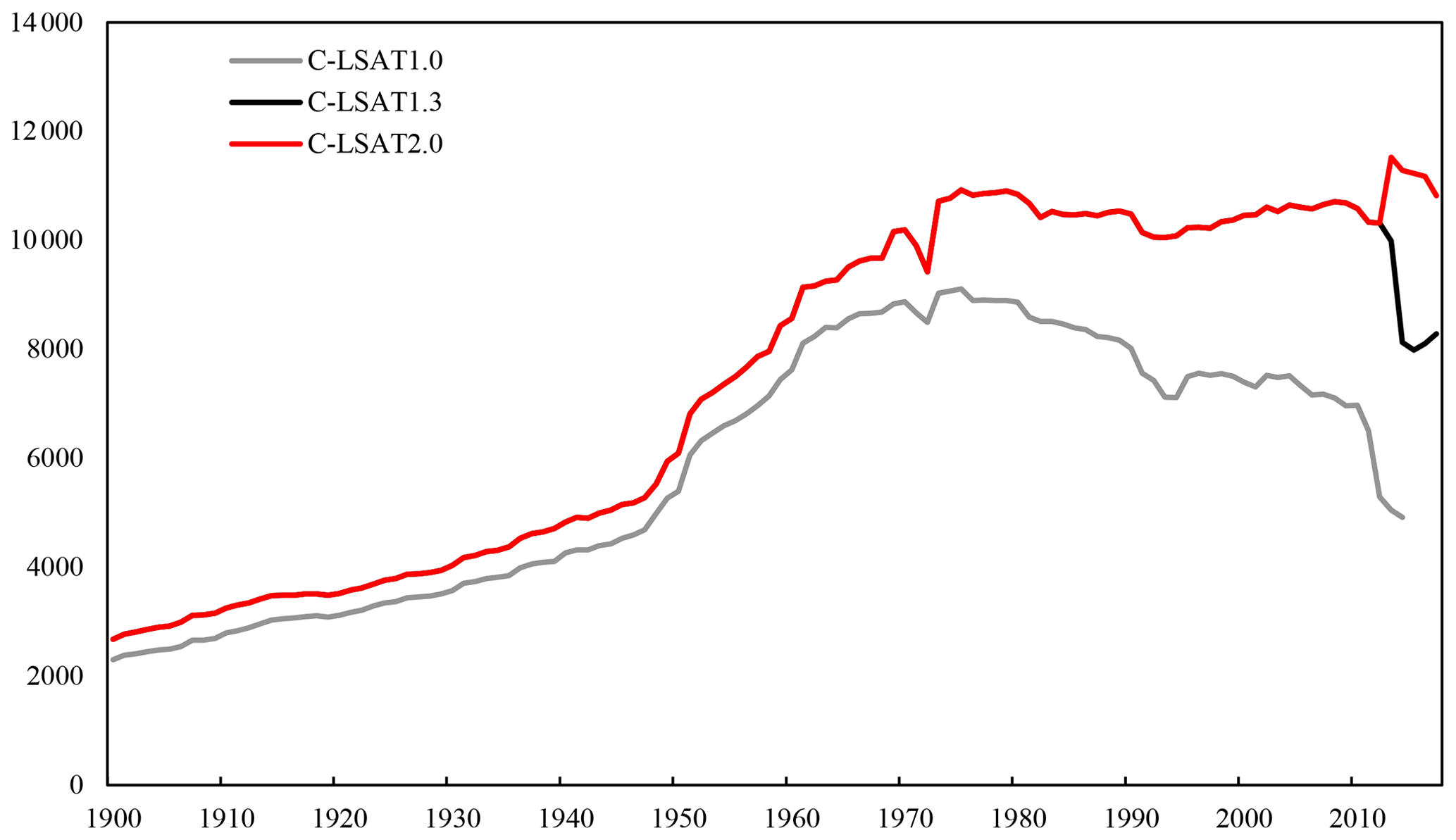
C-LSAT 2.0 used in this study is an update of C-LSAT 1.3. Compared to C-LSAT 1.3 from 1900 to 2017, version 2.0 is extended to 1850–2020, and there is a significant increase in the amount of in situ data for the period 2013–2017 (Fig. 1), with the increased in situ data from CLIMAT from the WMO's Global Telecommunication System (GTS) and Global Surface Daily Summary (GSOD) (https://www.ncei.noaa.gov/data/global-summary-of-the-day/archive/; last access: November 2021). It is homogenized using the same method as Xu et al. (2018). In addition, we have updated the data in C-LSAT2.0 for 2013–2019, which adds the number of in situ data in Africa, North America, and other regions in this study. The C-LSAT 2.0 dataset includes three temperature elements – monthly mean temperature, maximum temperature, and minimum temperature – and its time range for the three elements is January 1850–December 2020.

Figure 1 Comparison of C-LSAT 1.3 and C-LSAT 2.0 site counts from 1900 to 2017.

2.2 Sea surface temperature

CMST 1.0 (Yun et al., 2019) and CMST-Interim (Sun et al., 2021) use ERSSTv5 as the ocean component (Huang et al., 2017). ERSSTv5 starts from 1854, and we extend ERSSTv5 (1854–present) to 1850 using 1850–1853 SST anomalies (relative to 1961–1990 average) from ICOADS Release 3.0 (Freeman et al., 2017) and integrated into a global SST anomaly dataset for January 1850–December 2020. In the integrated SST dataset above, the SST is still set to a constant value of −1.8 ^∘C for areas with >90 % sea ice coverage as ERSSTv5. In addition, some areas in the high latitudes of the Southern Hemisphere (non-sea ice) are marked as missing values due to the lack of observations.

2.3 Sea ice surface air temperature

The common air temperature observation for the Arctic region is the International Arctic Buoy Program (IABP) (http://research.jisao.washington.edu/data_sets/iabppoles/; last access: October 2021), which contains oceanographic and meteorological observations for the Pacific Arctic, but it only has sea ice data from 1979 to the present, while the climate state of CMST is 1961–1990; the time length of IABP does not help us to estimate and reconstruct the temperature anomaly of the Arctic region in the CMST dataset, so we use the adjusted inverse distance weighted (AIDW; Cheng et al., 2020) extrapolation (site data) and EOT interpolation (gridding) methods to fill the default grid of the polar region (Cowtan and Way, 2014; Lenssen et al., 2019; Rohde and Hausfather, 2020; Vose et al., 2021).

3 CMST 2.0 reconstruction and uncertainty analysis

3.1 CMST and its brief reconstruction history

CMST 1.0 consists of C-LSAT 1.3 (1900–2017) as the terrestrial component and ERSSTv5 as the ocean component. The latest version without reconstruction is CMST 2.0 − Nrec in this study, which is composed of C-LSAT2.0 and ERSSTv5. Compared to CMST 1.0 from 1900–2017, CMST 2.0 − Nrec has been updated and expanded to 1850–2020. The original reconstructed version of CMST is the China global Merged Surface Temperature reconstruction dataset CMST-Interim, which is a merge of the reconstructed C-LSAT2.0 and ERSSTv5, where the reconstructed C-LSAT2.0 is an ensemble reconstruction dataset upgraded from C-LSAT2.0 (Li et al., 2021) with 756 ensemble members identified based on EOT and smoothing (Sun et al., 2021). Considering that there are many missing data due to sea ice coverage at high latitudes in the Northern Hemisphere in CMST, the AIDW extrapolation method is proposed to infill the missing data at some key sites; then the EOT interpolation method is used to reconstruct all the grid boxes over the sea-ice-covered region in this paper. Considering the effect of interannual variability in sea ice in the Arctic, 65–90^∘ N and 80–90^∘ N are taken as the assumed land components for ensemble reconstruction with C-LSAT 2.0, respectively, using the maximum sea ice area and minimum sea ice area for the entire period when satellite observations are available as a reference; then the ERSSTv5 ensemble reconstruction dataset is merged to generate CMST 2.0 − Imax and CMST 2.0 − Imin datasets.

3.2 Reconstruction of terrestrial and marine components

3.2.1 Reconstruction of the terrestrial component

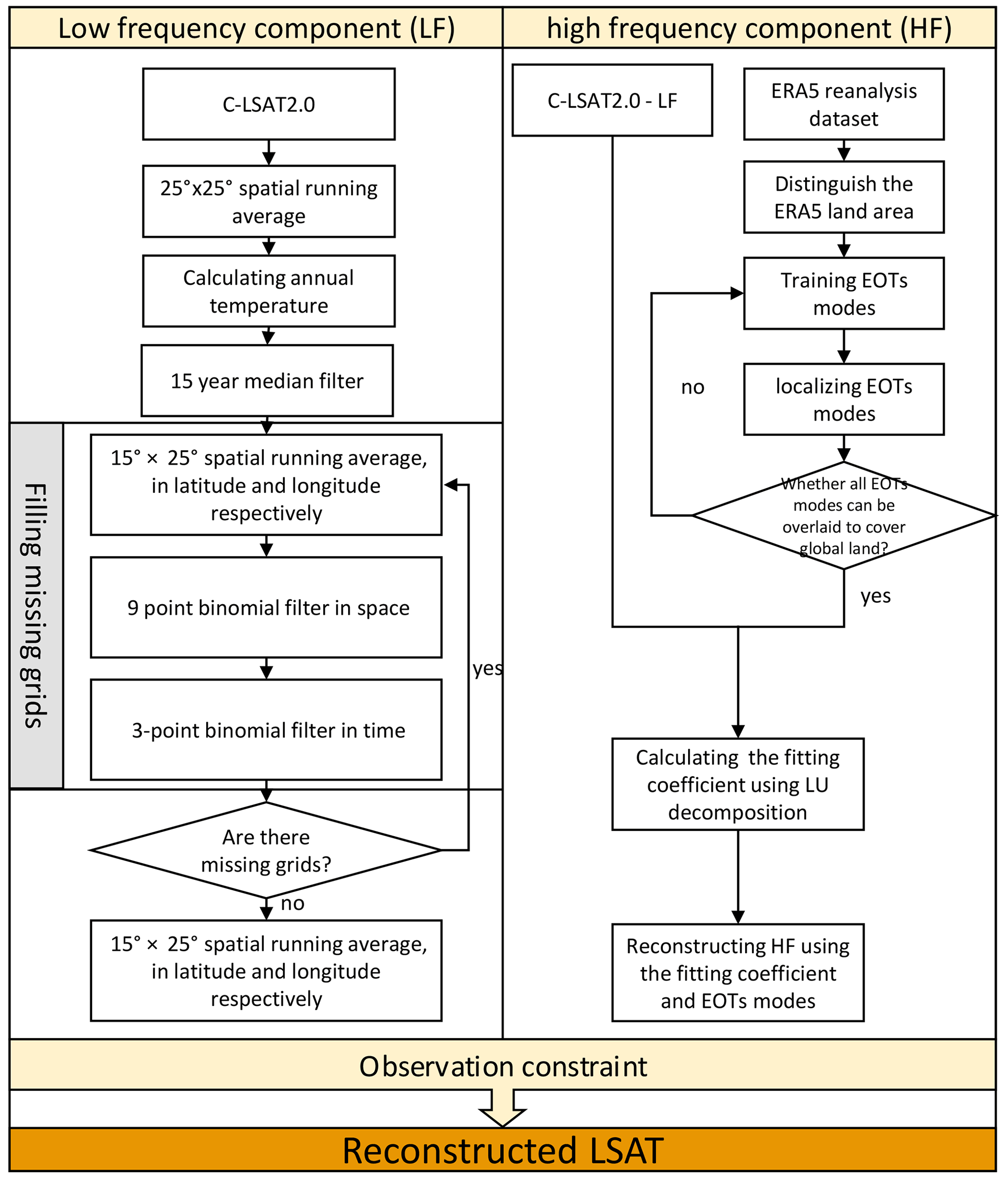
We follow the reconstruction method of CMST-Interim (Sun et al., 2021) and divide the C-LSAT 2.0 dataset into two parts, high- and low-frequency (HF and LF) components, for reconstruction, then sum them to obtain the reconstructed LSAT data (Fig. 2). The low-frequency component is a running average over time and space to characterize the large-scale features of LSAT anomalies in time and space. First, a 25^∘ × 25^∘ spatial running average is performed, and then the annual average of LSAT anomalies is calculated for at least 2 months of the year. Then, a 15-year median filter is used for the annual average LSAT, followed by a 15^∘ × 25^∘ spatial sliding average for latitude and longitude, respectively, as well as a nine-point binomial spatial filter and a three-point binomial temporal filter to fill in the default data. Finally, a 15^∘ × 25^∘ spatial running average is applied to latitude and longitude, respectively, to smooth the spatial distribution of the LSAT. The high-frequency component is the difference between the original data and the low-frequency component, characterizing the local variation in LSAT. We train the EOTs' modes using the ERA5 reanalysis dataset (Hersbach et al., 2020) (https://cds.climate.copernicus.eu/; last access: July 2020) and localize it. Afterward, the EOTs' modes are used to fit the high-frequency data to obtain a full-coverage reconstruction of the high-frequency component (Sun et al., 2021). The reconstructed land temperature data can be obtained by summing the low-frequency and high-frequency components, and finally, the reconstructed data are observationally constrained to remove the low-quality reconstructed data.

Figure 2 Schematic diagram of the LSAT reconstruction process.

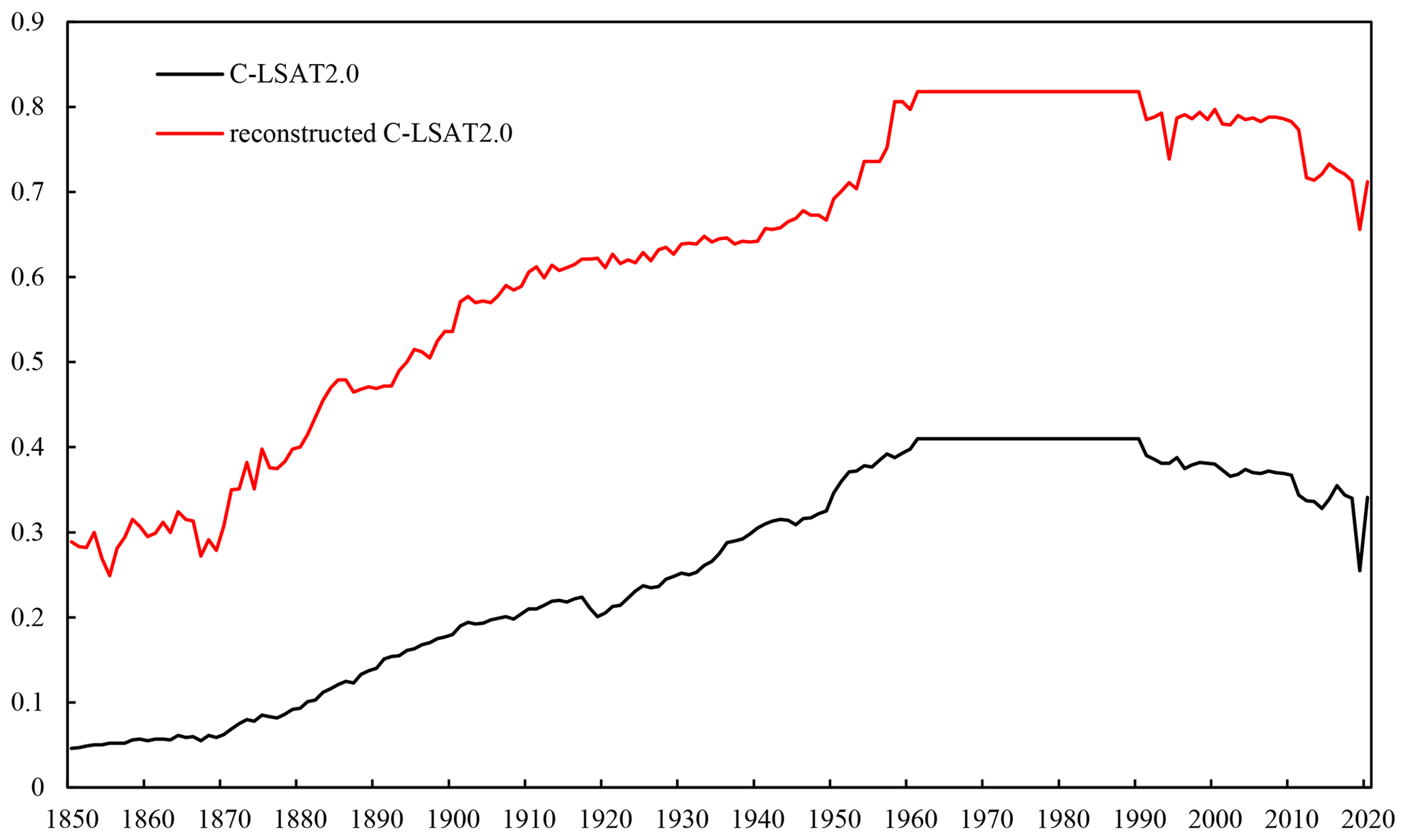
Reconstruction greatly improves the coverage of C-LSAT2.0. Figure 3 shows the comparison of land coverage before and after reconstruction. The land coverage of the reconstructed C-LSAT2.0 increases from the original 4.6 % in 1850 to 29 %, and the land coverage remains above 60 % after 1913 and reaches the maximum land cover of about 80 % in 1961, which last until 1990, after which it slightly decreases and remains at about 78 %. After 2012 there is a decreasing trend to about 70 %, where the land cover in 2019 is the lowest value of 66 % for the period 2012–2020; this is related to the lower number of sites in the year.

Figure 3 Coverage comparison of the terrestrial component before and after reconstruction.

3.2.2 Reconstruction of the ocean component

We use ERSSTv5 as the basis, which is a full-coverage, monthly reconstructed SST dataset based on observations from ships, buoys, and Argo (Huang et al., 2017). We fill the data during 1850–1853 with SST anomaly observed by ICOADS Release 3.0 (Freeman et al., 2017) to form a complete monthly SST anomaly dataset from 1850–2020 and then reconstruct it using the EOTs of Huang et al. (2017) to reduce the missing data.

3.3 Reconstruction of Arctic ice surface temperature

In CMST-Interim, when the Arctic is covered by sea ice, ERSSTv5 sets SST in the region with >90 % sea ice coverage to a constant value (−1.8 ^∘C), making surface temperature (ST) of CMST-Interim in the polar region the default value. It is worth noting that the Arctic is extremely sensitive to changes in climate forcing (polar amplification effect), so missing data in the polar regions in CMST-Interim may lead to an underestimation of the global warming trend (IPCC, 2021).

In order to solve this problem and improve the coverage of CMST in the Arctic, we improve the ST reconstruction method in the Arctic by expressing the ST of the Arctic in terms of the air temperature of the ice surface (considering the similar physical properties of ice and land, the sea ice is considered to be land). The month with the largest extent of Arctic sea ice is March, and the month with the smallest extent is September. According to the National Snow and Ice Data Center, during 1980–2020, the year with the largest sea ice extent in March is 1983, and the year with the smallest sea ice extent in September is 2012, so we designed two experiments: (1) CMST 2.0 − Imax uses 2 m air temperature to represent the temperature within the 65–90^∘ N region to simulate the ST of the Arctic sea-ice-covered region in March 1983, which is the maximum sea ice extent. (2) CMST 2.0 − Imin uses 2 m air temperature to represent the temperature within the 80–90^∘ N region to represent the ST in the Arctic sea-ice-covered region at the time of September 2012, which is the minimum sea ice extent (Fig. 4).

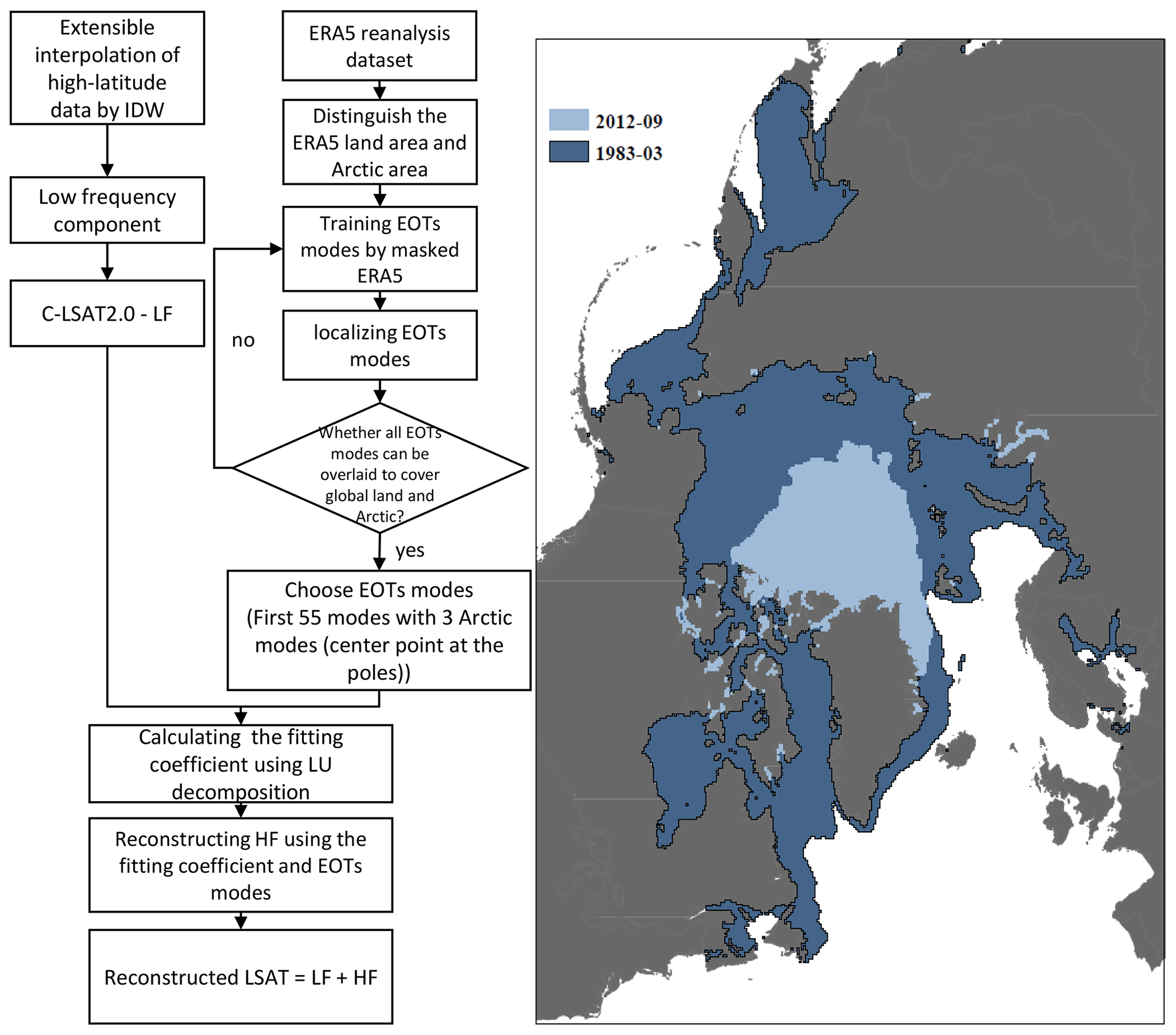
Figure 4 Reconstruction process of Arctic sea ice ST (left); comparison of maximum sea ice extent (sea ice extent in March 1983, shaded in dark blue) and minimum sea ice extent (sea ice extent in September 2012, shaded in light blue) distribution (right).

3.3.1 Maximum sea ice extent reconstruction CMST 2.0 − Imax

Due to the scarcity of observations in the Arctic and the fact that most observations were available after the 1980s, the observation period is very short. The data do not cover the entire period of 1961–1990, which is the climatology of our dataset. Therefore the observations cannot be added to the C-LSAT 2.0 dataset. Due to this fact, we use the AIDW to interpolate the data at lower latitudes to the Arctic (65–90^∘ N) and then perform the high- and low-frequency reconstruction method based on the interpolated dataset. It is worth noting that we included the region of 65–90^∘ N when training EOTs using the ERA5 reanalysis dataset. We selected the first 55 modes of the EOTs with three polar modes (the center point at the Arctic poles), for a total of 58 modes for reconstructing the high-frequency components (Fig. 4). After that, the reconstructed C-LSAT is merged with ERSSTv5, where the merged ERSSTv5 covers only the region south of 65^∘ N.

3.3.2 Minimum sea ice extent reconstruction CMST 2.0 − Imin

The reconstruction method of the terrestrial component in CMST 2.0 − Imin is consistent with CMST 2.0 − Imax, except that the merged process with ERSSTv5, in CMST 2.0 − Imin, the merged ERSSTv5 coverage is south of 80^∘ N. It is worth noting that the sea ice coverage range is 80–90^∘ N, and the region of 65–80^∘ N fills in SST in CMST 2.0 − Imin. However there are some grids in the region of 65–80^∘ N that are default values (caused by sea ice coverage) in ERSSTv5, so we use the AIDW method to fill these default grids.

Figure 5 shows the coverage comparison of CMST 2.0 − Nrec (without any land and ice air temperature reconstruction), CMST-Interim, CMST 2.0 − Imax, and CMST 2.0 − Imin. Overall, there is a significant improvement in the coverage of the reconstructed datasets compared to the original dataset, CMST 2.0 − Nrec. Globally, the coverage of CMST 2.0 − Imax and CMST 2.0 − Imin reconstructed for Arctic sea ice is consistently higher than CMST-Interim. CMST 2.0 − Imax and CMST 2.0 − Imin have the highest global coverage, with >80 % coverage after 1899. The global coverage of CMST-Interim reached more than 80 % after 1957. The comparative results for Northern Hemisphere coverage are primarily consistent with the global, with CMST 2.0 − Imax and CMST 2.0 − Imin having the greatest coverage, both reaching more than 90 % after the 1880s and CMST-Interim reaching 80 % coverage in 1901, but consistently below 90 %. In terms of global and Northern Hemisphere coverage, there are differences between CMST 2.0 − Imax, CMST 2.0 − Imin, and CMST-Interim, but the differences are not significant. However, the coverage of CMST 2.0 − Imax and CMST 2.0 − Imin differed significantly from CMST-Interim at high latitudes in the Northern Hemisphere, where the coverage of CMST-Interim has been below 70 % due to the existence of sea ice, while CMST 2.0 − Imax and CMST 2.0 − Imin reach full coverage at high latitudes in the Northern Hemisphere after 1983. There is no difference in the coverage of the three reconstructed datasets in other regions (Southern Hemisphere, Southern Hemisphere mid-high and low latitudes) except for the Northern Hemisphere and Northern Hemisphere high latitudes. The coverage of the reconstructed dataset in the Southern Hemisphere has improved considerably, with maximum coverage of about 80 %. The coverage of the reconstructed dataset in the high latitudes of the Southern Hemisphere is relatively small, consistently below 50 %, due to the scarcity of observations in Antarctica.

Figure 5 Coverage comparison of CMST 2.0 − Nrec, CMST-Interim, CMST 2.0 − Imax, and CMST 2.0 − Imin.

3.4 Estimation of uncertainty in the reconstructed CMST 2.0

Uncertainties in the reconstructed CMST 2.0 include both land and ocean uncertainties. The ocean uncertainty is the uncertainty in ERSSTv5. The land uncertainty is based on the reconstructed C-LSAT2.0 ensemble, which is divided into two parts: parameter uncertainty and reconstruction uncertainty. Since we reconstruct the temperature of the polar sea ice region in the way that we reconstruct the LSAT, we calculate the uncertainty in the 65–90^∘ N (Imax) and 80–90^∘ N (Imin) regions of CMST 2.0 − Imax and CMST 2.0 − Imin following the method of calculating the land uncertainty.

3.4.1 Parameter uncertainty in C-LSAT2.0 ensemble

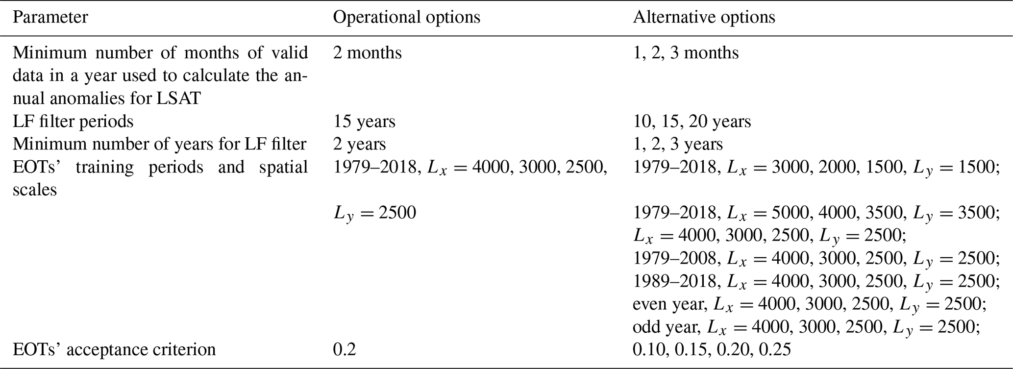
In the reconstruction process, we choose different parameters to generate 756-member ensembles (Table 1), which are different for different combinations, so the parameter uncertainty represents the difference in parameter combinations. According to Huang et al. (2020), the parameter uncertainty (U_p) is the regional average LSAT uncertainty, as follows:

$$\begin{array}{}\text{(1)}& {\displaystyle }{U}_{\mathrm{p}}^{\mathrm{2}}\left(t\right)={\displaystyle \frac{\mathrm{1}}{M}}\sum _{m=\mathrm{1}}^M[A_m^{\mathrm{g}}\left(t\right)-\stackrel{\mathrm{‾}}{A^{\mathrm{g}}}(t){]}^{\mathrm{2}}\text{(2)}& {\displaystyle }\stackrel{\mathrm{‾}}{A^{\mathrm{g}}}={\displaystyle \frac{\mathrm{1}}{M}}\sum _{m=\mathrm{1}}^M{A}_m^{\mathrm{g}}\left(t\right),\end{array}$$

where M is the total ensemble members ($m=\mathrm{1},\mathrm{2},\mathrm{\dots },M$), in this paper M=756; $A_m^{\mathrm{g}}$ represents global LSAT of the mth ensemble member; $\stackrel{\mathrm{‾}}{A^{\mathrm{g}}}$ is the average of all ensembles; and t represents temporal variations.

Table 1 Parameter settings used for reconstruction scenarios and the operational option.

Parameter uncertainties for the reconstructed C-LSAT2.0 ensemble, reconstructed C-LSAT2.0 + Imax (65–90^∘ N), and reconstructed C-LSAT2.0 + Imin (80–90^∘ N) show similar variations. The parameter uncertainties decrease over time, as does its interannual variability. The parameter uncertainties stabilize below 0.05 during 1876–2016 (Fig. 7). However, the parameter uncertainties are higher in 2018–2020 compared to the previous years. This is due to the lower coverage in this period compared to the last years, which is more sensitive to the parameter settings.

3.4.2 Reconstruction uncertainty in C-LSAT2.0 ensembles

In the reconstruction process, we smooth the observations when calculating the low-frequency component to filter out the short-term and local signals to obtain the large-scale characteristics of the LSAT anomaly, after which the high-frequency component is used to fit the local distribution of LSAT using the EOTs' spatial modes and the available observations. Our purpose of using EOTs is to obtain the spatial distribution of the LSAT anomaly, filter out the errors in the observations, and thus estimate the distribution of the LSAT anomaly from limited observations. However, the spatial pattern of EOTs also smoothes out the local temperature and ignores some local information, thus deviating from the observations. Therefore, according to Huang et al. (2016), we define the residual between the ideal observations and the reconstructed values using EOTs as the reconstruction uncertainty:

$$\begin{array}{}\text{(3)}& U_{\mathrm{r}}^{\mathrm{2}}\left(t\right)={\displaystyle \frac{\mathrm{1}}{M}}\sum _{m=\mathrm{1}}^M[R_m^{\mathrm{g}}\left(t\right)-D(t){]}^{\mathrm{2}},\end{array}$$

where D(t) represents the ideal observation, and $R_m^{\mathrm{g}}\left(t\right)$ is the reconstructed data obtained using the high- and low-frequency reconstruction method based on D(t).

The reconstruction uncertainty represents the differences between the ideal observations and the reconstructions. We choose two full-coverage CMIP6 models to represent the ideal observations to assess the deviation of the reconstructed values from the original values, which is due to missing information caused by the smoothing of local temperatures by EOTs. The C-LSAT 2.0 ensemble dataset covers the period 1850–2020, while the CMIP6 model historical experimental data are only available up to 2014, so we use model data from the SSP370 scenario (taking into account minor differences in the short term for any scenarios) to complement those of 2015–2020.

The two models we selected are BCC-CSM2-MR and GFDL-ESM4. BCC-CSM2-MR is a new version of the climate system model developed by the National Climate Center of China with improved parameterization and physical parameterization results. GFDL-ESM4 is an Earth system model developed by the GFDL model of the NOAA's Geophysical Fluid Dynamics Laboratory. Both models have a resolution of 1.125^∘ × 1.125^∘, and we descale both to 5^∘ × 5^∘ to calculate the temperature anomaly (1961–1990 climatology), after which the data from both models are reconstructed according to the high- and low-frequency reconstruction method.

Figure 6 shows the reconstruction uncertainties calculated using BCC-CSM2-MR and GFDL-ESM4. In general, the reconstruction uncertainties are relatively stable and do not increase over time. The reconstruction uncertainties in reconstructed C-LSAT2.0 + Imax and reconstructed C-LSAT2.0 + Imin are larger than that of reconstructed C-LSAT2.0, and the interannual variation is also larger. The interannual variability in the uncertainty in BCC-CSM2-MR is slightly smaller than that of GFDL-ESM4. In the following, we choose BCC-CSM2-MR as the reconstruction uncertainty to discuss the uncertainty in the terrestrial component.

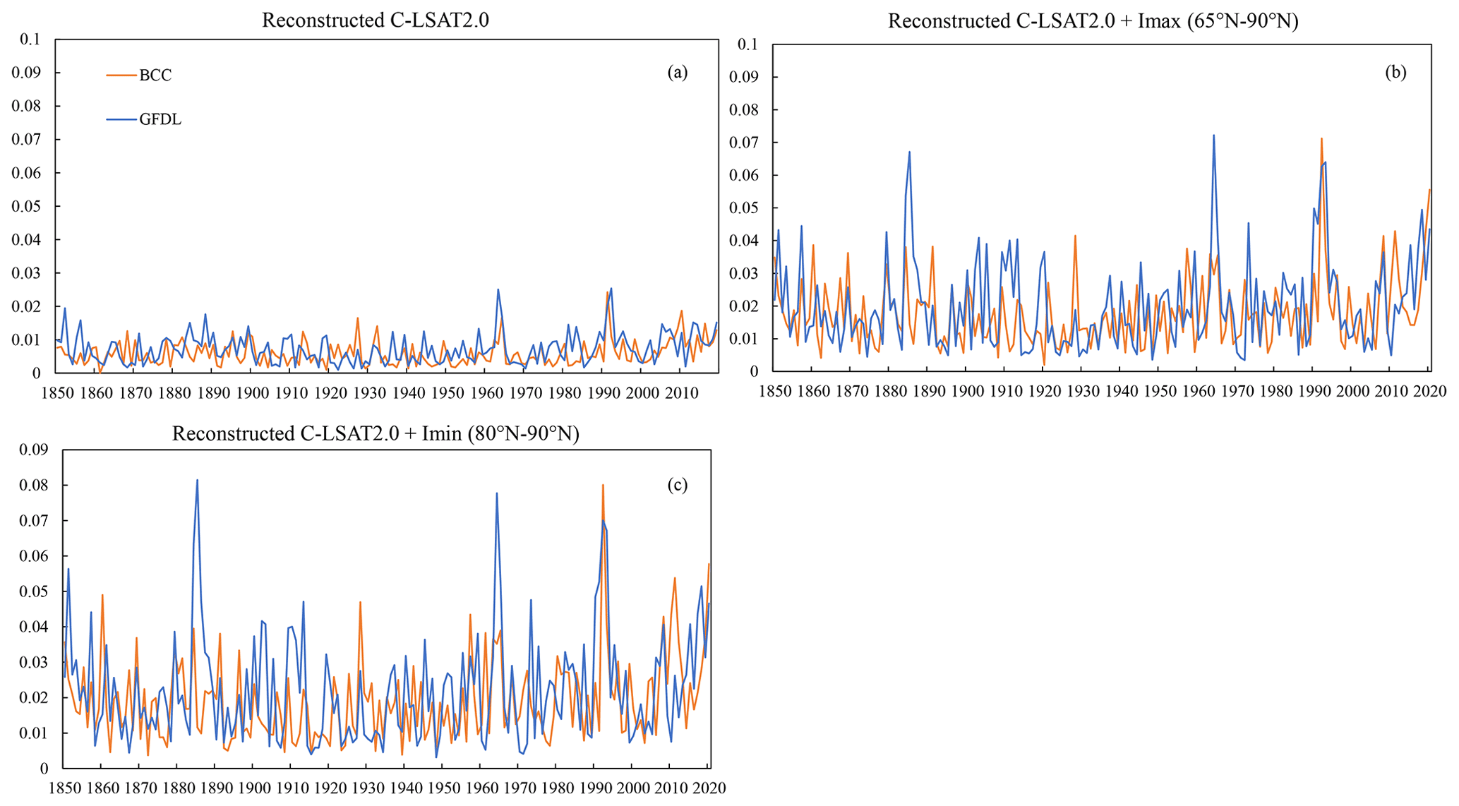
Figure 6 Reconstruction uncertainty in the reconstructed C-LSAT2.0 ensemble, reconstructed C-LSAT2.0 + Imax (65–90^∘ N), and reconstructed C-LSAT2.0 + Imin (80–90^∘ N) calculated using BCC-CSM2-MR and GFDL-ESM4.

3.4.3 Total uncertainty in LSAT

The total uncertainty in the C-LSAT2.0 ensemble is the sum of the parameter uncertainty and the reconstruction uncertainty:

$$\begin{array}{}\text{(4)}& U_{\mathrm{l}}^{\mathrm{2}}=U_{\mathrm{p}}^{\mathrm{2}}+U_{\mathrm{r}}^{\mathrm{2}}.\end{array}$$

Figure 7 shows the comparison of parameter uncertainty, reconstruction uncertainty, and total uncertainty in three C-LSAT2.0 ensemble datasets. The parameter uncertainties in the reconstructed C-LSAT2.0 ensemble, reconstructed C-LSAT2.0 + Imax (65–90^∘ N), and reconstructed C-LSAT2.0 + Imin (80–90^∘ N) are much larger than the reconstruction uncertainties before 1950, when the parameter uncertainties mainly determine the magnitude of total uncertainties. The difference between the parameter uncertainties and the reconstruction uncertainties from 1950 to 2016 becomes small, and both determine the total uncertainties. The total uncertainties increase after 2017 due to the increase in parameter uncertainties (Fig. 7a). The uncertainties in reconstructed C-LSAT2.0 + Imax and C-LSAT2.0 + Imin vary similarly (Fig. 7b and c). The parameter uncertainties in reconstructed C-LSAT2.0 − Imax and C-LSAT2.0 − Imin are larger than the reconstruction uncertainties before 1880, when the total uncertainties are dependent on parameter uncertainties. During 1880–1950, the magnitude of and variation in the parameter uncertainties and the reconstruction uncertainties are similar. After 1950, the parameter uncertainties decrease to less than the reconstruction uncertainties, during which reconstruction uncertainties determine the magnitude of and variation in the total uncertainties.

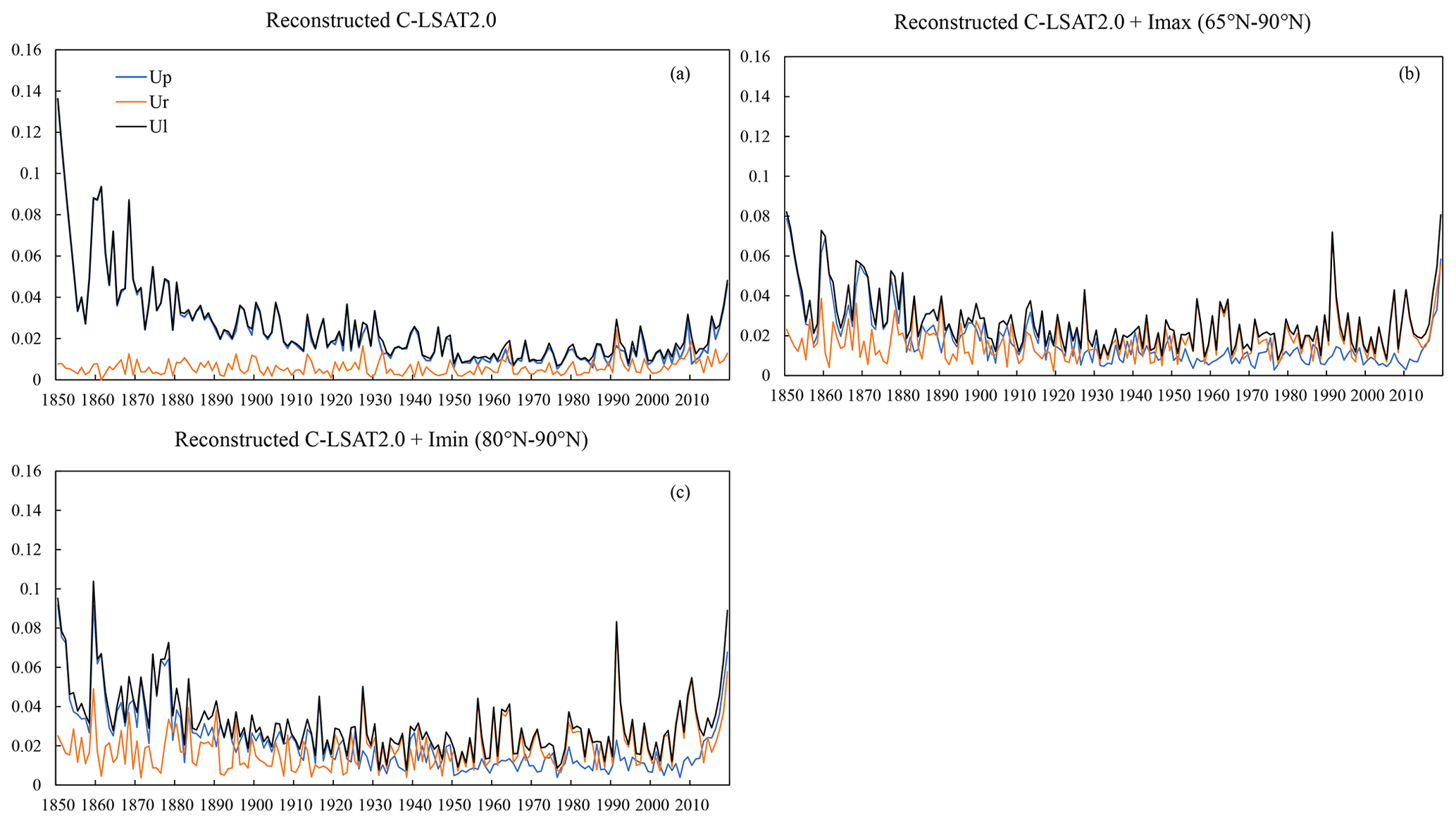
Figure 7 Parameter uncertainty, reconstruction uncertainty, and total uncertainty in three reconstructed C-LSAT2.0 ensembles.

3.4.4 Uncertainty in global surface temperature

The uncertainty in the global surface temperature consists of two components, the ocean component and the land component, and we calculate the total global temperature uncertainty as the sum of the two, based on the sea-to-land ratio, with the following formula:

$$\begin{array}{}\text{(5)}& U_{\mathrm{g}}^{\mathrm{2}}=a\times U_l^{\mathrm{2}}+b\times U_{\mathrm{s}}^{\mathrm{2}},\end{array}$$

where U_g represents the total uncertainty in GMST; U_l represents the uncertainty in global averaged LSAT, here chosen from the reconstructed C-LSAT2.0; U_s represents the uncertainty in global averaged ocean component, here chosen from the ERSSTv5 (since the uncertainty in ERSSTv5 is only calculated up to 1854, our uncertainty in GST forward also only covers up to 1854); a and b are constants, which are the proportion of land and ocean area to the globe, respectively, but since the uncertainty in the reconstructed Arctic region in CMST 2.0 − Imax and CMST 2.0 − Imin is calculated according to the land uncertainty, a=0.32 and b=0.689 in CMST 2.0 − Imax, and a=0.30 and b=0.70 in CMST 2.0 − Imin.

Figure 8 shows uncertainties in the GMST, land component, and ocean component for CMST-Interim (a), CMST 2.0 − Imax (b), and CMST 2.0 − Imin (c). The variation in GMST uncertainty is similar for the three datasets, but the interannual variation in GMST uncertainty for CMST 2.0 − Imax and CMST 2.0 − Imin is larger than CMST-Interim, especially after 1994, when both the magnitude and interannual variation in GMST uncertainty for CMST 2.0 − Imax and CMST 2.0 − Imin are significantly greater than CMST-Interim (Fig. 8d). Uncertainties in the ocean and land components have generally declined, and thus the uncertainty in GMST has also reduced (Fig. 8a–c). Before 1870, the uncertainties in land and ocean component are similar, but the interannual variability in the land uncertainty is greater than that of the ocean. During 1871–1986, the uncertainty in the ocean component is larger than the uncertainty in the land component, and the uncertainty in GMST depended mainly on the uncertainty in the ocean component, and the interannual variability was consistent with the ocean component. There are two peaks in global uncertainty during this period, in the late 1910s and early 1940s, consistent with ocean uncertainty. The peaks in ocean uncertainty are associated with the two world wars, and the uncertainty is larger due to the smaller observation coverage of the SST during the war period (Huang et al., 2020). Between 1986 and 2003, the uncertainty in GST was determined by both the land and ocean components. After 2003, the magnitude of uncertainty in the ocean component is smaller than that of the land component, and the land component determines the magnitude of the uncertainty in GST, and the interannual variation is also consistent with the land component.

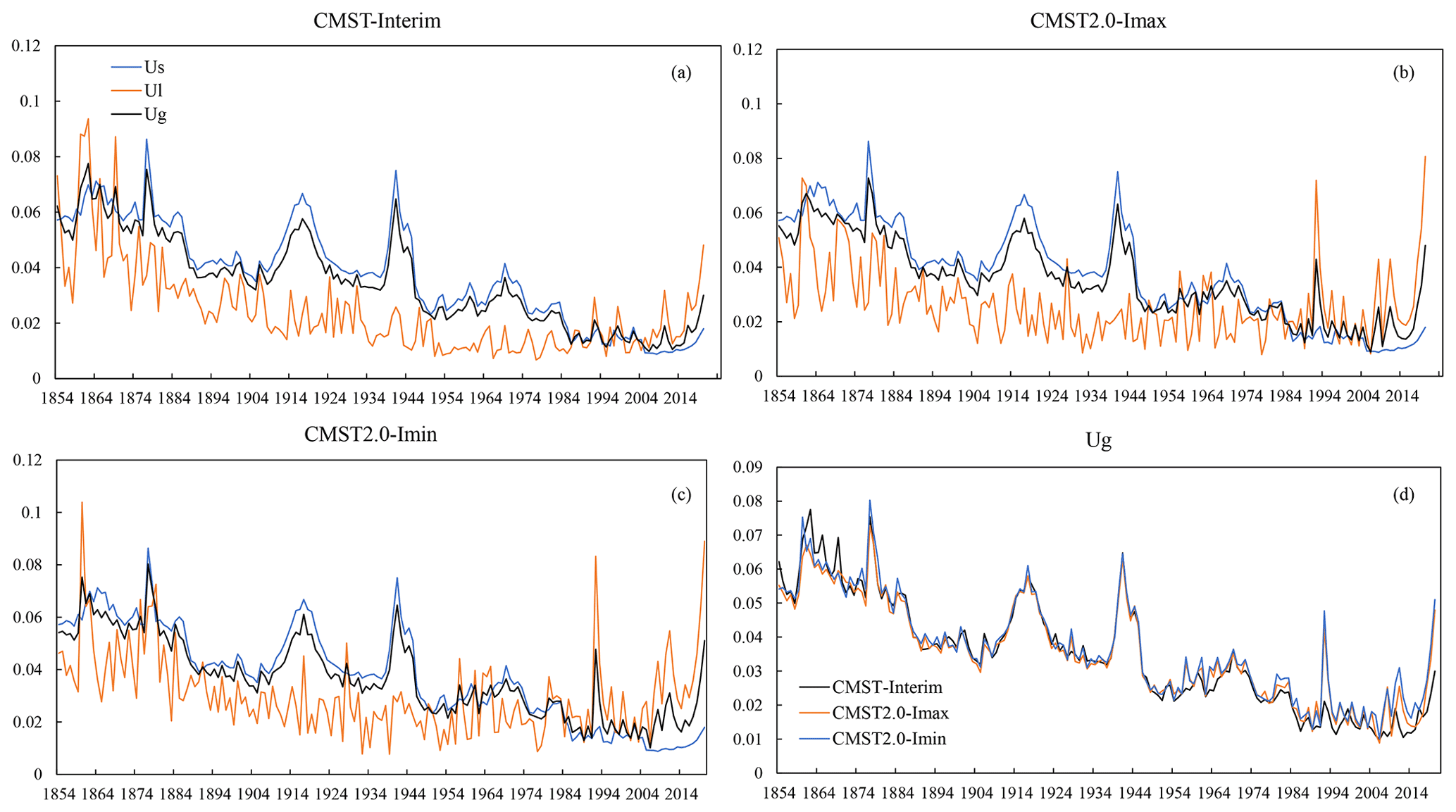
Figure 8 Uncertainties in GMST (U_g), LSAT (U_l), and SST (U_s) for CMST-Interim (a), CMST 2.0 − Imax (b), and CMST 2.0 − Imin (c) and their comparison of U_g (d).

4 Composition of C-LSAT2.0 and CMST 2.0

The C-LSAT2.0 datasets consist of two datasets, C-LSAT2.0 and reconstructed C-LSAT2.0, while each dataset includes three temperature-related elements, including monthly average, maximum, and minimum temperatures.

The CMST 2.0 datasets consist of three versions: CMST 2.0 − Nrec, CMST 2.0 − Imax, and CMST 2.0 − Imin (Table 2).

CMST 2.0 − Nrec is the observation-based homogenized gridded dataset, consisting of C-LSAT2.0 and ERSSTv5, where the uncertainty in C-LSAT2.0 is not estimated, and the uncertainty in ERSSTv5 consists of parameter uncertainty and reconstruction uncertainty.

CMST 2.0 − Imax is based on the CMST-Interim gridded dataset with the addition of Arctic reconstruction (65–90^∘ N), including reconstructed C-LSAT2.0 with the addition of Arctic reconstruction (65–90^∘ N) and ERSSTv5 with 90^∘ S–65^∘  N. Its uncertainties include the terrestrial uncertainty and the oceanic uncertainty, where the terrestrial uncertainty is the uncertainty in the reconstructed C-LSAT2.0 and of the reconstructed surface air temperature (SAT) over the ice surface, including the parameter uncertainty and the reconstruction uncertainty, and the oceanic uncertainty is derived from the uncertainty in ERSSTv5 (Huang et al., 2017).

Similarly, CMST 2.0 − Imin is the gridded data, which modify the reconstructed Arctic region based on CMST 2.0 − Imin. The modification part is to reduce the reconstructed Arctic region of C-LSAT2.0 to 80–90^∘ N and expand the merged ERSSTv5 to 90^∘ S–80^∘ N area.

Table 2 Composition of CMST 2.0 datasets and CMST-Interim.

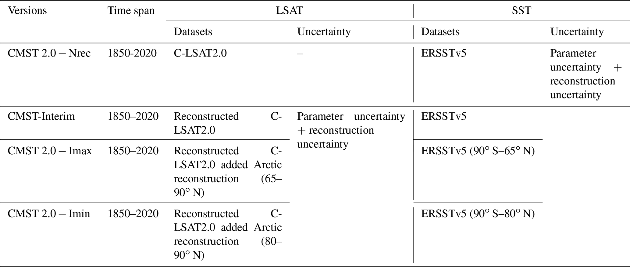
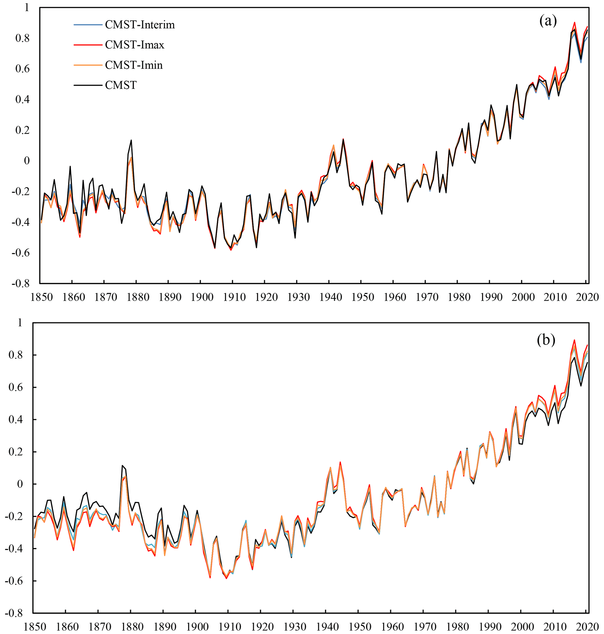
Figure 9 Comparison of GMST anomaly series (relative to 1961–1990 average) for CMST 2.0 datasets and CMST-Interim using two methods: (a) calculated based on the weighted average of global mean LSAT and SST series according to the sea–land ratio, (b) calculated based on latitudinal weighting.

5 The GMST series of CMST 2.0 datasets

Comparing the GMST series of CMST 2.0 datasets and CMST-Interim shows that the variability in GMST in the reconstructed datasets is generally consistent with CMST 2.0 − Nrec (Fig. 9). We also compare the GMST series for the four datasets calculated by the two methods, which is similar for the three reconstructed datasets (CMST-Interim, CMST 2.0 − Imax, and CMST 2.0 − Imin) and differs slightly for the unreconstructed dataset CMST 2.0 − Nrec (Fig. 9a and b). The warming of CMST − Nrec in Fig. 9b is significantly lower than that in Fig. 9a, which is related to the lower land coverage. The LSAT coverage of CMST 2.0 − Nrec is low in previous decades and is below 18 % before 1900 (Fig. 3), so the GMST series is susceptible to the influence of ocean temperature, making the GMST series high; The LSAT coverage of CMST 2.0 − Nrec has increased in recent decades, with terrestrial coverage above 70 % (Fig. 3), but the coverage is low at high latitudes, in South America, and Africa, where the absence of LSAT, especially at high latitudes and in the Arctic, makes the GMST series low. It can be seen that the warming rate of CMST 2.0 − Nrec calculated using latitude weighting will be significantly lower, so we are using the sea–land ratio method to calculate the warming trend when comparing each dataset in the following.

In Fig. 9a, the CMST-Interim, CMST 2.0 − Imax, and CMST 2.0 − Imin GMST series are lower than CMST − Nrec before the 1880s, which is mainly due to the lower coverage of observations in this period, making the interannual variability in the GMST series in CMST 2.0 − Nrec larger, while the reconstructed datasets filled in part of the default grids, resulting in higher coverage and thus lower interannual variability in GMST series. The reconstructed datasets show high agreement with the CMST − Nrec temperature series and its interannual variability as the coverage of the observations increased after the 1880s. While the GMST series of CMST 2.0 − Imax is significantly higher than the other three datasets after the 2000s because CMST 2.0 − Imax reconstructs the Arctic region, and the polar amplification effect of the Arctic significantly increases the GMST series, the GMST series of CMST-Interim and CMST 2.0 − Imin are essentially the same as CMST − Nrec, but CMST 2.0 − Imin is slightly higher than CMST-Interim because CMST 2.0 − Imin fills the 80–90^∘ N region with ice surface temperatures, while CMST-Interim uses SST. The GMST series of CMST 2.0 − Imax and CMST 2.0 − Imin are higher than CMST-Interim after 2000, indicating that the influence of polar temperature on global temperature also increases with global warming. In summary, the warming trends of the reconstructed datasets for 1850–2020 are all higher than CMST 2.0 − Nrec (0.05±0.003 ^∘C per decade, with CMST 2.0 − Imax having the most significant warming trend (0.054±0.003 ^∘C per decade) and CMSR2.0 − Imin the second-largest (0.053±0.003 ^∘C per decade) (Table 4). The warming trend estimated by CMST-Interim is 0.051±0.003 ^∘C per decade, which is slightly larger than CMST − Nrec, mainly due to the lower temperature series before the 1880s, excluding this period, and the warming trend from 1880 to 2020 estimated by CMST-Interim (0.073±0.003 ^∘C per decade) is consistent with CMST − Nrec (0.073±0.004 ^∘C per decade) (Table 4), while the warming trends of CMST 2.0 − Imax and CMST 2.0 − Imin are higher than the previous two datasets, 0.076±0.004 ^∘C per decade and 0.074±0.003 ^∘C per decade (Table 4), respectively, due to the polar amplification effect.

Table 3 General information of input datasets.

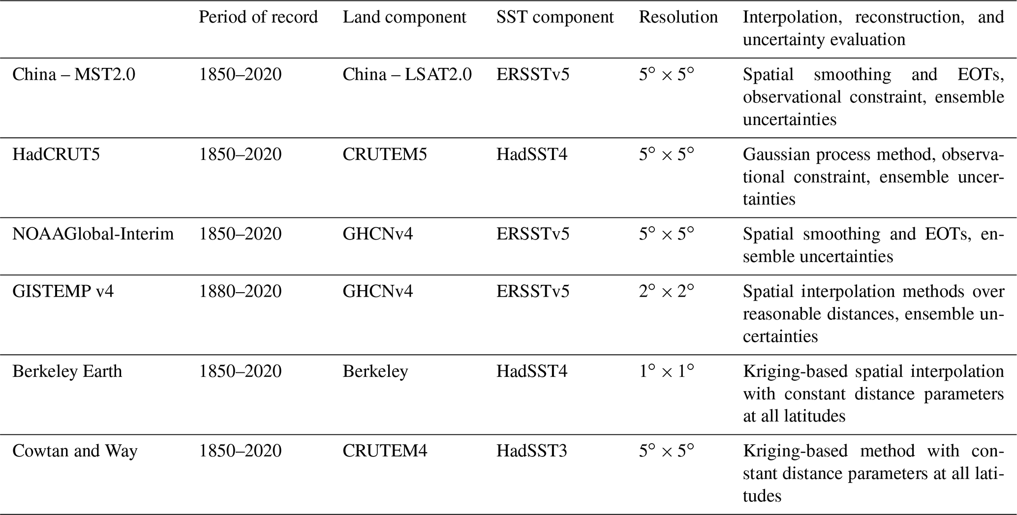
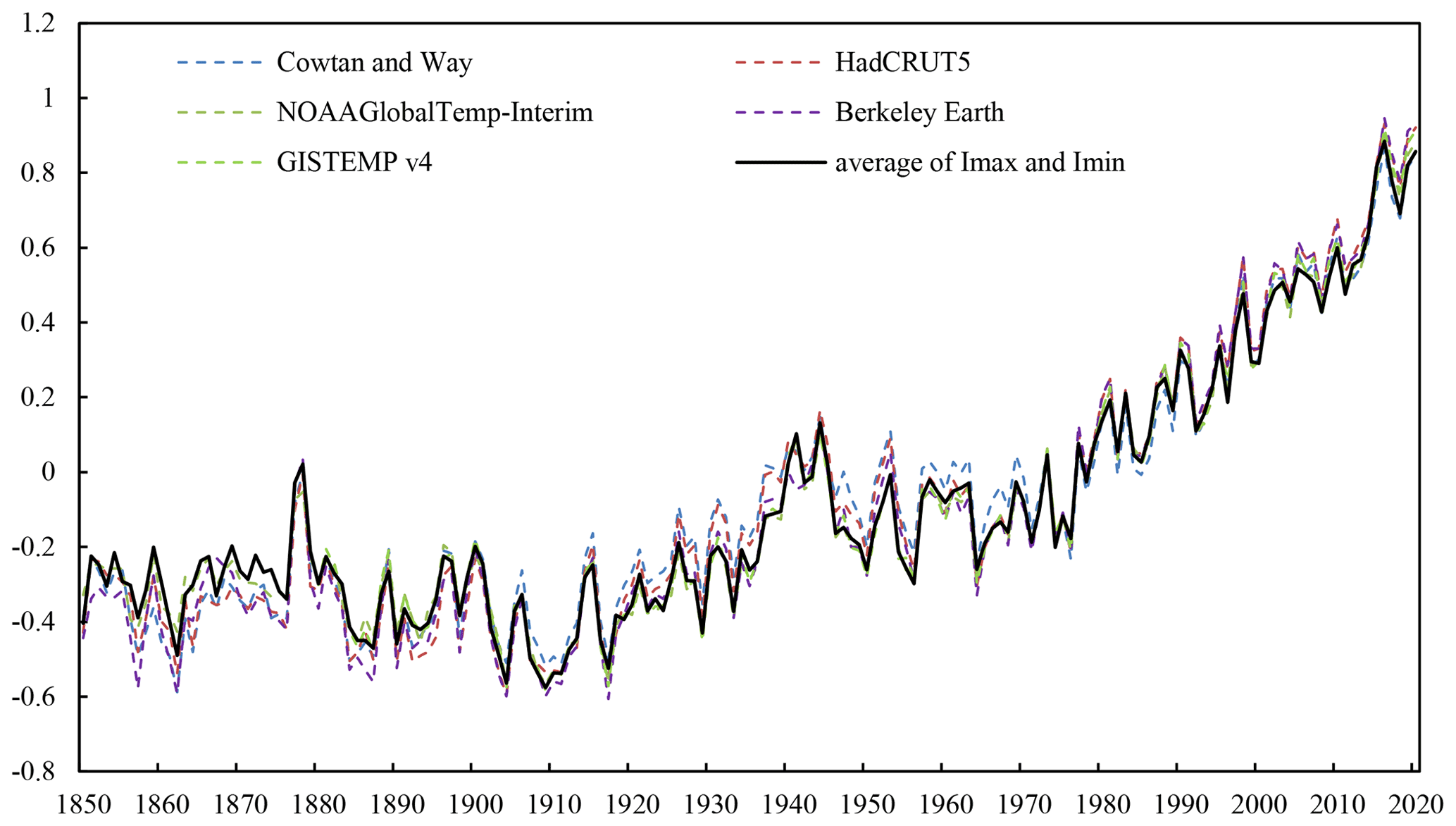
Figure 10 Comparison of GMST anomaly series (relative to 1961–1990 average) for different datasets. The GMST anomaly series calculated based on the weighted average of global mean LSAT and SST series according to the sea–land ratio. The average of Imax and Imin is the average of GMST series of CMST 2.0 − Imax and CMST 2.0 − Imin.

6 Comparison of CMST 2.0 − Imax and CMST 2.0 − Imin with other datasets

Figure 10 shows the GMST series of CMST 2.0 compared with the other datasets (Table 3). The GMST series of the seven datasets (CMST 2.0 includes two variants of Imax and Imin) are generally consistent. The GMST series of CMST 2.0 − Imax and CMST 2.0 − Imin are similar to the other five datasets, indicating that their estimated Arctic temperature variation is consistent with the other datasets, and can accurately reflect the impact of the Arctic amplification effect on GST. Due to sparse observations, the variability between datasets is high until the 1880s, as is the interannual variability between datasets. After the 1900s, the GMST series of CMST 2.0 − Imax and CMST 2.0 − Imin are generally lower than other datasets. In the 1910s–1970s, the Cowtan–Way dataset is consistently higher than other datasets. In the 1930s–1950s, HadCRUT5 is higher than the other datasets but similar to Cowtan–Way. After the 2000s, the CMST 2.0 datasets are generally lower than other datasets, with CMST 2.0 − Imax being closer to the NOAAglobalTemp-Interim GMST series. For the period 1850–2020, the warming trend of CMST 2.0 − Nrec is the lowest (0.05±0.003 ^∘C per decade), and the highest (0.062±0.003 ^∘C per decade) warming trend is Berkeley in the seven datasets. The warming trend of CMST-Interim is consistent with HadCRUT5, both at 0.051±0.003 ^∘C per decade. The warming trend of CMST 2.0 − Imax is the same as NOAAglobalTemp-Interim (0.054±0.003 ^∘C per decade). Between 1880 and 2020, CMST 2.0 − Nrec (0.073±0.004 ^∘C per decade) is in agreement with CMST-Interim (0.073±0.003 ^∘C per decade), CMST 2.0 − Imax is consistent with NOAAglobalTemp-Interim (0.076±0.004 ^∘C per decade), and CMST 2.0 − Imin (0.075±0.003 ^∘C per decade) is consistent with Cowtan–Way (0.074±0.003 ^∘C per decade) (Table 4). We also calculate the warming trends of different datasets for different periods – 1900–2020, 1951–2020, 1979–2020, and 1998–2020 – and found that the warming rate becomes faster over time for most of the datasets; especially the increasing warming trend for 1998–2020 is much larger than the other periods, indicating that the global warming rate is accelerating. The maximum warming trend of 0.228±0.029 ^∘C per decade (GISTEMP v4) during 1998–2020 increased by 0.037±0.017 ^∘C per decade compared to the warming trend during 1979–2020. The largest increasing warming trend is NOAAglobalTemp-Interim, with a warming trend of 0.037±0.017 ^∘C per decade for 1998–2020, which is 0.04 ^∘C per decade higher than the warming trend during 1979–2020, followed by CMST 2.0 − Imax, CMST 2.0 − Imin, and Berkeley Earth. CMST 2.0 − Nrec and CMST-Interim have relatively small increases in the warming trend. The relatively large increases in warming trend estimated in most datasets with reconstructed Arctic temperatures, compared to those without (CMST 2.0 − Nrec and CMST-Interim), illustrate the impact of polar amplification on global warming and reflect the importance of reconstructing Arctic default data.

Table 4 Warming trends for different datasets during different periods. The GMST series used to calculate the warming trend is calculated based on the weighted average of global mean LSAT and SST series according to the sea–land ratio.

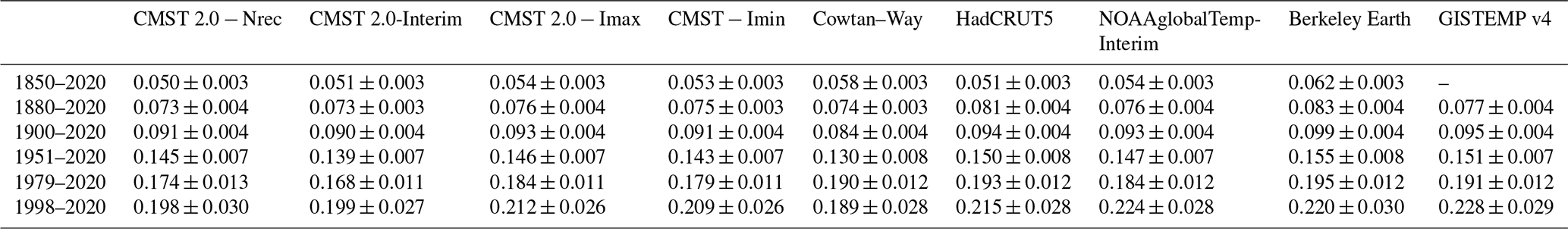
Figure 11 Distribution of warming trends estimated from different datasets during 1880–2020.

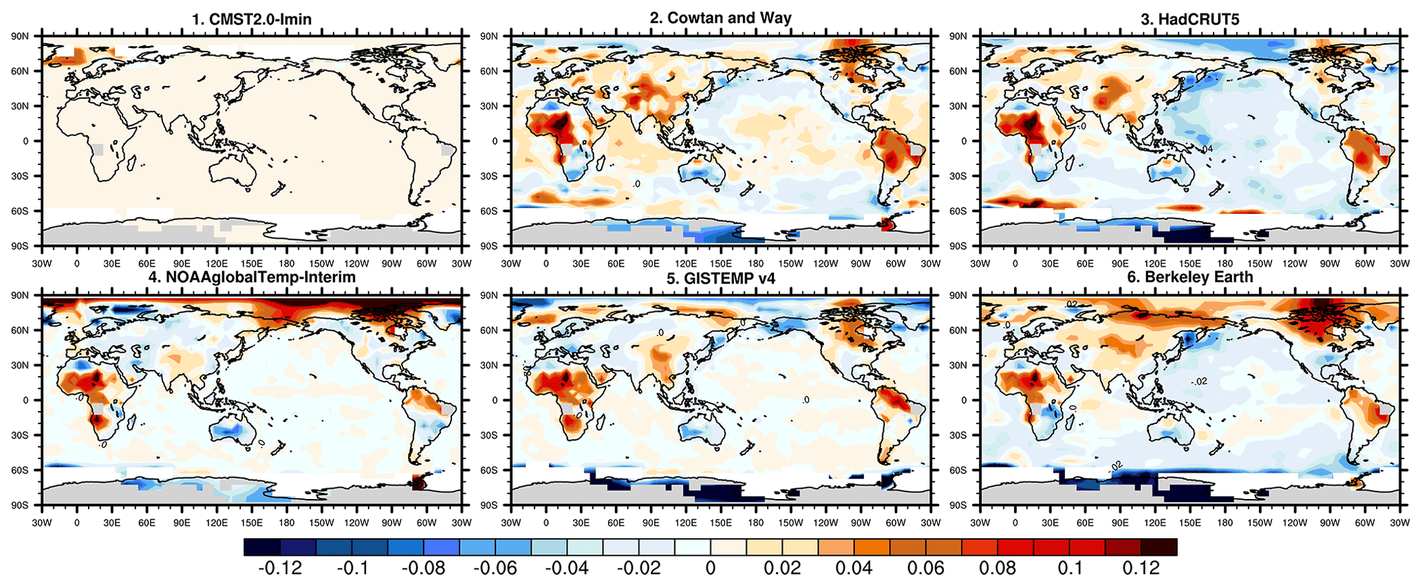
Figure 12 Differences in warming trends estimated by six other datasets (including CMST 2.0 − Imin) and CMST 2.0 − Imax.

Figure 11 compares the distribution of warming trends for different datasets for 1880–2020. The distribution of warming trends is relatively consistent among the nine datasets, except for the Antarctic, with a zone of high warming values in central Asia, Europe, and northeastern North America. There are large differences among the datasets in the Antarctic region due to the sparse observations. CMST-Interim, CMSR2.0 − Imax, and CMST 2.0 − Imin have fewer LSATs in the Antarctic due to the sparse observations and observational constraints. Except for CMST 2.0 − Nrec, the estimated warming trends of the other eight datasets clearly increase with latitude in the Northern Hemisphere region. Most datasets assess a significantly higher warming trend in the Arctic (60–90^∘ N) than in the lower latitudes. Except for the CMST 2.0 − Nrec and CMST-Interim datasets, in which Arctic temperature is not available, the magnitude of the estimated Arctic warming trend for 1880–2020 is similar (Fig. 12). Still, the warming trends near the poles differ significantly, with more significant warming trends estimated by HadCRUT5 and GISTEMP v4. CMST 2.0 − Imax, CMST 2.0 − Imin, Cowtan–Way, and Berkeley Earth have similar warming trends, while NOAAglobalTemp-Interim has the smallest warming estimate near the poles. CMST 2.0 − Imax, HadCRUT5, and GISTEMP v4 all show a high warming trend in the high latitudes of North America and the northwestern Arctic Ocean, but CMST 2.0 − Imax has a relatively small range of highs. Cowtan–Way and Berkeley Earth are similar to the former three datasets but have smaller ranges and magnitudes. Meanwhile, each dataset also has a range of warming highs in the southeastern Arctic Ocean; NOAAglobalTemp-Interim estimates the most extensive range of warming; and CMST 2.0 − Imax, CMST 2.0-Min, HadCRUT5, and GISTEMP v4 estimate similar ranges of warming. In addition, all datasets, including CMST 2.0 − Nrec and CMST-Interim, have low warming trend near Scandinavia. The analysis of the warming trends in the Arctic shows that the magnitude and spatial distribution of the warming trends estimated based on CMST 2.0 − Imax and CMST − Imin are more consistent with the other datasets. Therefore, they are reasonable for the spatial interpolation reconstruction of temperature anomalies in the Arctic.

7 Data availability

The C-LSAT2.0 datasets are currently publicly available at the website of figshare under the DOI https://doi.org/10.6084/m9.figshare.16968334.v4 (Sun and Li, 2021b), which contains monthly mean, maximum, and minimum temperature before and after reconstruction during 1850–2020.

The CMST 2.0 datasets can be downloaded at https://doi.org/10.6084/m9.figshare.16929427.v4 (Sun and Li, 2021a), which contains CMST 2.0 − Nrec, CMST-Interim, CMST 2.0 − Imax, and CMST 2.0 − Imin datasets.

These datasets are also available freely at http://www.gwpu.net (last access: January 2022).

8 Summary and prospects

This paper describes the composition and construction process of the latest versions of the C-LSAT 2.0 and CMST 2.0 ensemble datasets. The C-LSAT 2.0 datasets consist of the C-LSAT 2.0 gridded dataset and the reconstructed C-LSAT 2.0 dataset, including three meteorological elements: monthly average, maximum, and minimum temperatures. The CMST 2.0 datasets consist of the CMST 2.0 − Nrec gridded dataset and two reconstructed datasets (including CMST 2.0 − Imax and CMST 2.0 − Imin). The CMST 2.0 datasets contain the monthly average temperature anomaly. The resolution of all datasets is 5^∘ × 5^∘, and the time range is 1850–2020. The reconstructed C-LSAT 2.0 dataset, reconstructed according to the high- and low-frequency reconstruction method in Sun et al. (2021), is merged with ERSSTv5 to generate the global surface temperature ensemble dataset CMST-Interim. CMST 2.0 − Imax and CMST 2.0 − Imin are based on CMST-Interim, combining AIDW and high- and low-frequency reconstruction methods for temperature reconstruction in the Arctic. Compared with the unreconstructed dataset CMST 2.0 − Nrec, the coverage of the reconstructed datasets is greatly improved. These two datasets have greatly improved coverage in the Northern Hemisphere due to the reconstruction in the Arctic. Compared to 60 %–70 % for CMST 2.0 − Nrec before 1910, the coverage of CMST-Interim has improved to 75 %–85 %, and CMST 2.0 − Imax and CMST 2.0 − Imin are both above 80 %. The coverage of CMST 2.0 − Imax and CMST 2.0 − Imin in the Northern Hemisphere is 80 %–99 %, and CMST-Interim is 65 %–87 %. There was no difference in coverage between the three reconstructed datasets in the Southern Hemisphere.

We then systematically evaluate the uncertainty in the reconstructed datasets. The results of the uncertainty assessment of the reconstructed C-LSAT2.0 show that the magnitude of the reconstruction uncertainty is generally smaller than that of the parameter uncertainty, and the parameter uncertainty mainly determines the total uncertainty in the LSAT. The uncertainty in the reconstructed LSAT is similar to previous estimates (Li et al., 2020; Sun et al., 2021). The uncertainty in reconstructed C-LSAT2.0 + Imax and reconstructed C-LSAT2.0 + Imin is relatively consistent with the uncertainty variation in reconstructed C-LSAT2.0, but the interannual variation is larger, and the increasing trend of parameter uncertainty in reconstructed C-LSAT2.0 + Imax and reconstructed C-LSAT2.0 + Imin is significantly higher than that of reconstructed C-LSAT2.0 after 2017. The uncertainty analysis of CMST 2.0 shows that the uncertainty in GST depends mainly on the oceanic component before 1986, is determined by both oceanic and terrestrial components during 1986–2003, and depends on the magnitude of the terrestrial component after 2003.

Results comparing the GMST series of the three CMST 2.0 datasets and CMST-Interim show that the reconstructed datasets improve the estimation of global warming trends while increasing data coverage, especially for the datasets that include the Arctic region in the reconstructed area. Compared with 0.05±0.003 ^∘C per decade and 0.073±0.004 ^∘C per decade for CMST 2.0 − Nrec, CMST 2.0 − Imax and CMST 2.0 − Imin estimated warming trends of 0.054±0.003 and 0.053±0.003 ^∘C per decade for 1850–2020, and 1880–2020 is 0.076±0.004 and 0.075±0.003 ^∘C per decade, with a very significant increase. Compared with the five datasets in IPCC AR6, it can be found that the datasets considering the reconstruction of Arctic sea ice temperature can more accurately reflect the effect of polar amplification on global temperature. The GMST series and warming trends estimated by CMST 2.0 − Imax and CMST 2.0 − Imin are more consistent with these five datasets. Both have similar estimates of the spatial distribution and magnitude of warming trends in the Arctic as the other datasets.

The current CMST 2.0 dataset for the Arctic is a reconstruction of the sea ice surface temperature in a defined region (65–90^∘ N or 80–90^∘ N) with 2 m air temperature. Although the influence of Arctic temperature on global temperature is considered, and the change in GMST series is estimated relatively accurately, it still cannot reflect the impact of sea ice dynamics on global temperature very accurately. Therefore, our future work will gradually consider the dynamics of sea ice as much as possible in the reconstruction process in order to more accurately estimate and analyze the amplification effect of the Arctic and its impact on GMST.

Last but not least, due to the limited observations, it is very difficult to fully reconstruct the SATs over the Antarctic and the surrounding SSTs during the earlier periods (for example, prior to the 1950s), which means the CMST 2.0 is still not “full-coverage”. This will need to be better addressed by continuing to supplement data sources and technically refine methods in future studies.