Implementation of the CCDC algorithm to produce the LCMAP Collection 1.0 annual land surface change product

The increasing availability of high-quality remote sensing data and advanced technologies has spurred land cover mapping to characterize land change from local to global scales. However, most land change datasets either span multiple decades at a local scale or cover limited time over a larger geographic extent. Here, we present a new land cover and land surface change dataset created by the Land Change Monitoring, Assessment, and Projection (LCMAP) program over the conterminous United States (CONUS). The LCMAP land cover change dataset consists of annual land cover and land cover change products over the period 1985–2017 at a 30 m resolution using Landsat and other ancillary data via the Continuous Change Detection and Classification (CCDC) algorithm. In this paper, we describe our novel approach to implement the CCDC algorithm to produce the LCMAP product suite composed of five land cover products and five products related to land surface change. The LCMAP land cover products were validated using a collection of ∼25 000 reference samples collected independently across CONUS. The overall agreement for all years of the LCMAP primary land cover product reached 82.5 %. The LCMAP products are produced through the LCMAP Information Warehouse and Data Store (IW+DS) and shared Mesos cluster systems that can process, store, and deliver all datasets for public access. To our knowledge, this is the first set of published 30 m annual land change datasets that include land cover, land cover change, and spectral change spanning from the 1980s to the present for the United States. The LCMAP product suite provides useful information for land resource management and facilitates studies to improve the understanding of terrestrial ecosystems and the complex dynamics of the Earth system. The LCMAP system could be implemented to produce global land change products in the future. The LCMAP products introduced in this paper are freely available at https://doi.org/10.5066/P9W1TO6E (LCMAP, 2021).

1 Introduction

Changes in land cover and land surface are one of the greatest and most immediate influences on the Earth system, and these changes will continue in association with a surging human population and growing demand on land resources (Szantoi et al., 2020). Changes in land cover and ecosystems and their implications for global environmental change and sustainability are major research challenges for developing strategies to respond to ongoing global change while meeting development goals (Turner et al., 2007). Unknowns related to the spatial extent and degrees of impacts of anthropogenic activities on natural systems and strategies to respond to ongoing global change hinder efforts to overcome sustainability challenges (Erb et al., 2017; Reid et al., 2010). An improved understanding of the complex and dynamic interactions between the various Earth system components, including humans and their activities, is critical for policymakers and scientists (Foley et al., 2005, 2011). To fully understand these processes and monitor these changes, accurate and frequently updated land cover information is essential for scientific research and to assist decision makers in responding to the challenges associated with competing land demands and land surface change.

The characteristics of land surface fundamentally connect with the functioning of Earth's terrestrial surface. Satellite observations have been used to observe the Earth's surface and to characterize land cover and change from local to global scales. Remote sensing data allow us to obtain information over large areas in a practical and accurate manner. With advanced technologies and accumulating satellite data, countries and regions have produced multi-spatial-resolution and multi-temporal-resolution land cover products (Chen et al., 2015; Gong et al., 2020; Hansen et al., 2013; Homer et al., 2020; Li et al., 2020). A variety of land change mapping has been carried out to produce land cover and change products in the United States. Among these efforts are the widely known National Land Cover Database (NLCD) products. NLCD has provided comprehensive, general-purpose land cover mapping products at a 30 m resolution since 2001 in the United States, and the products have been published and updated across more than a decade (Homer et al., 2020). NLCD provides Anderson Level II land cover classification (Anderson, 1976) for the conterminous United States (CONUS) at approximately 2–3-year intervals. Other national-scale mapping projects focus on specific land cover themes. Among these are the Landscape Fire and Resource Management Planning Tools (LANDFIRE) (Picotte et al., 2019), which maps vegetation and fuels in support of wildfire management, and the Cropland Data Layer (Boryan et al., 2011) generated by the National Agricultural Statistics Service (NASS) of the United States Department of Agriculture (USDA). Due to the need to incorporate data from neighboring years, as well as extensive post-processing, ancillary dataset dependencies, and analyst-supported refinement, release dates for both LANDFIRE and NLCD products are typically several years subsequent to the nominal map year. Other products including national urban extent change and vegetation phenology data are available (Li et al., 2019, 2020). These projects vary in how land change information is incorporated or expressed across product releases. Continuous data stacks allow for an increase in input features for land cover classification. Frequent data also provide the opportunity for near-real-time change monitoring with frequently updated image acquisitions. The availability of land change information has led to approaches that attempt to monitor surface properties continuously through time (Franklin et al., 2015; Gong et al., 2019; Hermosilla et al., 2018; Homer et al., 2020; Kennedy et al., 2015; Li et al., 2020). Such approaches have several advantages over traditional image processing techniques based on small numbers of images (Bullock et al., 2020; Zhu and Woodcock, 2014b).

Leveraging the increasingly massive number of openly available, analysis-ready data products into the generation of operational land cover and land change information has been described as the new paradigm for land cover science (Wulder et al., 2018). The approach, which intended to use all available medium-resolution remotely sensed data from the 1980s to the present, opened a door for the scientific community to integrate time series information to improve change detection and land cover characterization in a robust way. Furthermore, change events, when combined with knowledge of ecology settings or anticipation of a given process post-change, can accommodate consistent change observations and characterization of land cover. For example, forest areas that are cleared by wildfire or harvest activities typically transfer to non-forest herbaceous or shrub vegetation cover, followed by a succession of young tree stages and ultimately returning to a forest class. Traditional change detection methods using limited observations may not have identified these changes if data were collected with a starting date prior to the change and an end date that occurred after the transitional (non-tree) vegetation returned to tree cover. Therefore, incorporating change information into the land cover characterization process allows for insights regarding expected land cover class transitions related to successional processes and likewise provides a mechanism to identify illogical class transitions and causes or agents of change (Kennedy et al., 2015; Wulder et al., 2018). The choice of a time series approach also allows missing data and phenological variations to be handled robustly (Friedl et al., 2010; Wulder et al., 2018).

The Continuous Change Detection and Classification (CCDC) algorithm (Zhu and Woodcock, 2014b; Zhu et al., 2015b) was developed to advance time series change detection by using all available Landsat data. The Continuous Change Detection (CCD) algorithm uses robust methodology to identify when and how the land surface changes through time. The algorithm first estimates a time series model based on clear observations and then detects outliers by comparing model estimates and Landsat observations. The algorithm fits harmonic regression models through a least absolute shrinkage and selection operator (LASSO) (Tibshirani, 1996) approach to every pixel over time to estimate the time series model defined by sine and cosine functions. New Landsat records are compared to predicted results, and if the observed data deviate beyond a set threshold for all records within a moving window period, then a model break is produced. The parameters used to fit the model are used as inputs for the cover classifier for land cover characterization.

The original implementation of CCDC was written in the MATLAB programming language and had been implemented for a regional land cover change assessment in the eastern CONUS (Zhu and Woodcock, 2014b). The algorithm includes the automation of change detection and classification and can monitor changes for different land cover types. The implementation of CCDC over a large geographic extent still encounters several challenges: the availability of Landsat records and training datasets, the effectiveness of choosing good-quality Landsat records, and the robustness to characterize land cover and change across various land cover types and conditions. In this paper, we outlined major efforts and challenges in the implementation of CCDC for the US Geological Survey (USGS) Land Change Monitoring, Assessment, and Projection (LCMAP) initiative (Brown et al., 2020). LCMAP focuses on using CCD/CCDC with Landsat time series records and other ancillary information to produce annual land cover and change products from 1985 to the present for the United States. We focused on how LCMAP employed every observation in a time series of US Landsat Analysis Ready Data (ARD) (Dwyer et al., 2018) over a long period starting with the 1980s to determine whether change occurred at any given point in the observation record. The CCDC algorithm that was initially developed for abrupt change detection on the land surface was modified through lessons learned from the prototype test to include both gradual land cover transition and abrupt land change so that the algorithm could be used in an operational setting with the goals of robust, repeatable, and geographically consistent results (Brown et al., 2020). The algorithm was further used to classify the pixel to indicate what land cover type or types were observed before and after a detected change on the land surface. Classification in LCMAP was modified to improve representativeness of training data and reduce notable artifacts including misclassification of rare classes and dramatic increases in the number of training data. The CCDC algorithm has since been translated into an open-source library as Python code. The full implementation joined the CCD Python library with the classification methodology in combination with data delivery/processing services made available through the LCMAP Information Warehouse and Data Store (IW+DS) and evolved as a national operational monitoring system.

2 Data sources

The CCDC algorithm utilizes all available Landsat observations including surface reflectance, brightness temperature, and associated quality data to characterize the spectral responses of every pixel through harmonic regression model fits. The model fits are then used to categorize each pixel time series into temporal segments of stable periods and to estimate the dates at which the spectral time series data diverge from past responses or patterns. The outcomes of model fits and other input data are then used for classification. The algorithm requires several input datasets to perform both change detection and classification.

2.1 Landsat observations

US Landsat ARD have been processed according to a minimum set of requirements and organized into a form that can be more directly and easily used for monitoring and assessing landscape change with minimal additional user effort. Landsat ARD Collection 1 provides consistent radiometric and geometric Landsat products across Landsat 4–5 Thematic Mapper (TM), Landsat 7 Enhanced Thematic Mapper Plus (ETM+), and Landsat 8 Operational Land Imager (OLI)/Thermal Infrared Sensor (TIRS) instruments for use in time series analysis (Dwyer et al., 2018). Landsat ARD is organized in tiles, which are units of uniform dimension bounded by static corner points in a defined grid system (Fig. 1). An ARD tile is currently defined as 5000 × 5000 pixels of 30 m or 150 × 150 km. To implement CCDC algorithms to produce LCMAP Collection 1.0 land change products in CONUS, all available Landsat ARD records of surface reflectance and brightness temperature from the 1980s to 2017 were required.

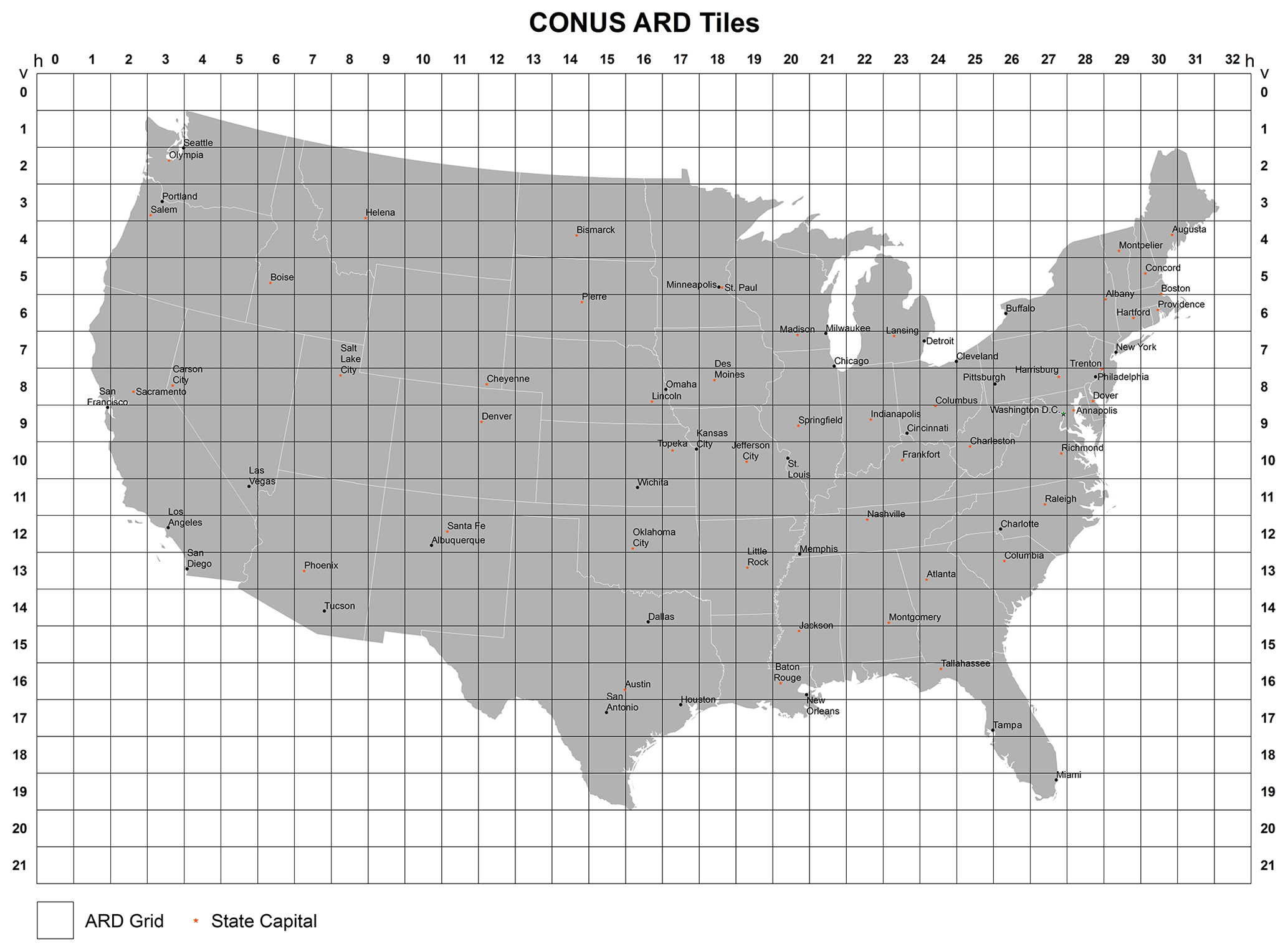
Figure 1 Landsat ARD tile grids for the conterminous USA.

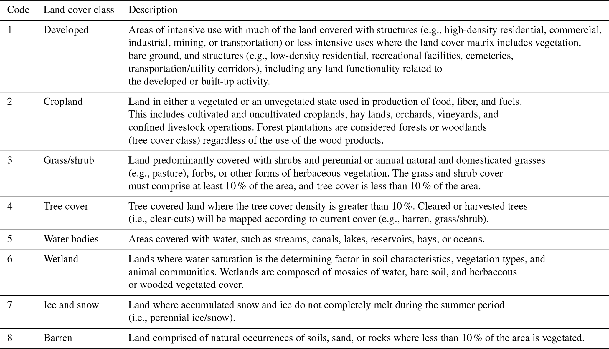
2.2 Land cover and ancillary datasets

The CCDC algorithm employs every observation in a time series of Landsat data to determine whether change has occurred at any given time. The algorithm further classifies the time series to indicate what land cover types were observed before and after a detected change and further to generate LCMAP annual land cover products (Table 1). The land cover products are produced by using training data from NLCD in 2001. NLCD provides Anderson Level II (Anderson, 1976) land cover classification for CONUS and outlying areas (Homer et al., 2020). Spectral index and change metrics between cloud-corrected Landsat mosaics are used, among other information, to identify change pixels (Jin et al., 2013). These metrics allow NLCD to incorporate temporal and spectral trajectory information into both training data selection and final land cover classification. The NLCD land cover data are used in LCMAP as land cover training data.

Table 1 LCMAP land cover product specifications.

Ancillary data comprise two main source datasets: the USGS National Elevation Dataset (NED) (Gesch et al., 2002) 1 arcsec digital elevation models (DEMs) and a wetland potential index (WPI) layer created for NLCD 2011 land cover production (Zhu et al., 2016). The WPI layer is a ranking (0–8) of wetland likelihood from a comparison of the National Wetlands Inventory (NWI), the US Department of Agriculture Soil Survey Geographic Database (SSURGO) for hydric soils, and the NLCD 2006 wetlands land cover classes.

3 Methodology

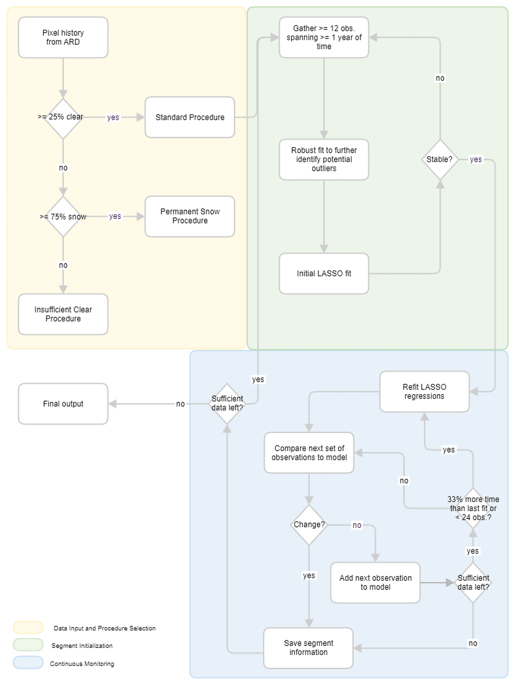
As part of the operational LCMAP system, the original MATLAB version of the CCDC algorithm is converted to a format that meets the needs of large-scale land change detection and change characterization on an annual basis. Python is selected to replace MATLAB to implement the CCDC algorithm for LCMAP. The CCD component of the CCDC algorithm is converted to create the Python-based CCD (PyCCD) library. The PyCCD library is a per-pixel algorithm, and the fundamental outputs are the spectral characterizations (segments) of the input data. There are several key components in PyCCD. The overall CCD procedures are summarized in Fig. 2.

Figure 2 Overall procedures of the CCD algorithm.

3.1 Data filtering and harmonic modeling

The removal of invalid and cloud-contaminated data points is important for deriving model coefficients that accurately represent the phenology of the surface and for the correct identification of model break points. The CCD algorithm uses Landsat ARD PIXELQA values to mask observations identified as cloud, cloud shadow, fill, or (in some cases) snow derived based on the Fmask 3.3 algorithm (Zhu et al., 2015a; Zhu and Woodcock, 2012). Additional cirrus and terrain occlusion bits are provided for Landsat 8 OLI–TIRS ARD that are not available in the Landsat 4–7 TM/ETM+ quality assessment band. To maintain consistency across the historical archive, the algorithm does not rely on these Landsat 8-only quality assurance (QA) flags to filter out observations.

Landsat ARD containing invalid or physically unrealistic data values are removed. For the surface reflectance bands, the valid data range is between 0 and 10 000. Brightness temperature values, which in the ARD are stored as 10× temperature (kelvins), are converted to 100× (^∘C), and observations are filtered for values outside the range −9320 to 7070 (−93.2 to 70.7 ^∘C). This procedure rescales the brightness temperature values into a roughly similar numerical range to that of the surface reflectance bands. A multi-temporal mask (Tmask) model (Zhu and Woodcock, 2014a) is implemented first to remove additional outliers by using the multi-temporal observation record to identify values that deviate from the overall phenology curve using a specific harmonic model to perform an initial fit to the phenology. Additional details are provided in Eq. (S1) in the Supplement.

The filtered Landsat ARD are further operated upon to generate the time series fit by harmonic models whose sinusoidal components are frequency multiples of the base annual frequency. A constant and linear term characterizes the surface reflectance or brightness temperature offset value and overall slope, respectively. The full harmonic model is defined as follows:

$$\begin{array}{}\text{(1)}& \widehat{p}(i,t)=c_{\mathrm{0},i}+c_{\mathrm{1},i}t+{\sum }_{n=\mathrm{1}}^{\mathrm{3}}\left(a_{n,i}\cos \mathit{\omega }nt+b_{n,i}\sin \mathit{\omega }nt\right),\end{array}$$

where ω is the base annual frequency $(\mathrm{2}\mathit{\pi }/T)$, t is the ordinal of the date when 1 January of the year zero has ordinal 1 (sometimes called Julian date), i is the ith Landsat band, a_n, i and b_n, i are the estimated nth order harmonic coefficients for the ith Landsat band, c_0, i and c_1, i are the estimated intercept and slope coefficients for the ith Landsat band, and $\widehat{p}(i,t)$ is the predicted value for the ith Landsat band at ordinal date t. Model initialization and certain special-case regression fits such as at the beginning/end of the time series use the simple four-coefficient model. Outside of these conditions, the selection of coefficients depends on the number of observations used for the regression. For a full model (eight coefficients), there must be at least 24 observations covered by the regression. The fit parameters returned by PyCCD always include eight coefficient values including an intercept, with unused coefficients reported as zeroes.

3.2 Regression models and change detection thresholds

The best-fit coefficients for the time series model are calculated using a LASSO regression model (Tibshirani, 1996). In contrast to ordinary least squares (OLS), which was used in the original CCDC development, LASSO penalizes the sum of the absolute values of coefficients, in some cases forcing a subset of the coefficients to zero. Together with the explicit limits enforced on the number of coefficients, this reduces instances of overfitting, including in cases when observations are too sparse or unevenly distributed in time to constrain the model to real phenological features. To detect change, the LASSO model checks CCD model breaks with respect to its last determined best-fit harmonic model.

To correctly detect change, the algorithm distinguishes between a substantive deviation from model prediction and deviations that result from variability inherent in the data (due to incomplete atmospheric removal and/or other sources of natural variation) to detect change. The algorithm calculates two parameters related to dispersion, or scatter, to estimate the variability in data for each spectral band. The first one is a comparison root-mean-square error (RMSE) that is the RMSE of the 24 observations covered by the model which are closest in day of year to the last observation in the “peek window” or over all observations covered by the model if there are fewer than 24. This value is recalculated at each step of the time series. The second parameter (var) is used to measure the overall variability in the data values and is defined as the median of the absolute value of the differences between each observation and the ith successive observation, where i is the smallest value such that the majority of these observation pairs are separated by more than 30 d if possible (otherwise, i=1). The var is computed once at the beginning of the standard procedure, using all non-masked observations in the time series.

Observations not yet incorporated into the model are evaluated as a group of no fewer than the PEEK_SIZE parameter value; this is the peek window, which “slides” along the time series one observation at a time. For each iteration, a value is calculated for each individual observation within the peek window as follows:

$$\begin{array}{}\text{(2)}& {\text{mag}}_n=\sum _{i\in D}{\left({\displaystyle \frac{{\text{resid}}_{n,i}}{max\left({\text{var}}_i,{\text{RMSE}}_i\right)}}\right)}^{\mathrm{2}},\end{array}$$

where resid_n, i is the residual relative to the LASSO models for each band i and for each observation n within the PEEK_SIZE window and var_i and RMSE_i are the parameters of dispersion as described above, for each band i. This summation is carried out for all bands i in the set of DETECTION_BANDS (D). This produces a scalar magnitude, representing the deviation from model prediction across these bands, for each observation. The detection of a model break requires this value to be above the CHANGE_THRESHOLD value for all observations in the window. This is separate from the value that is reported as a per-band magnitude when a change is detected in the time series. Change detection sensitivity depends on the value of the change threshold. The CHANGE_THRESHOLD is determined in Eqs. (S2) and (S3) in the Supplement. If mag_n< CHANGE_THRESHOLD for any n in the PEEK_SIZE window, then add the most recent observation to the segment by shifting the PEEK_SIZE window one observation forward in the time series. If mag_n> CHANGE_THRESHOLD for all n values in the PEEK_SIZE window, this is considered a spectral break.

3.3 Permanent snow and insufficient clear observation procedures

The permanent snow procedure indicates that too few clear (fewer than 25 % of total observations) or water observations, which are identified from the QA band, exist to robustly detect change and a large fraction of observations are snow. The algorithm will return at most one segment that fits through the entire time series and provide at least 12 filtered observations. The model will, under the default settings, fit only four coefficients (i.e., characterizing the reflectance and brightness temperature bands using only a simple harmonic with no higher-frequency terms). Unlike other procedures, snow pixels are not filtered out and are fit as part of the annual pattern. This avoids overfitting the model to a seasonally sparse observation record. Similarly, for the insufficient clear observations determined by the QA band, the model will perform a LASSO regression fit for the entire time series using four coefficients. The model coefficients and RMSE from this regression are recorded. Additional parameters including the start, end, and observation count are also saved. Further, the change Boolean value is set to 0, and the break day is recorded as the last observation date. The magnitude of change as zero for each band is also saved.

3.4 Land cover classification

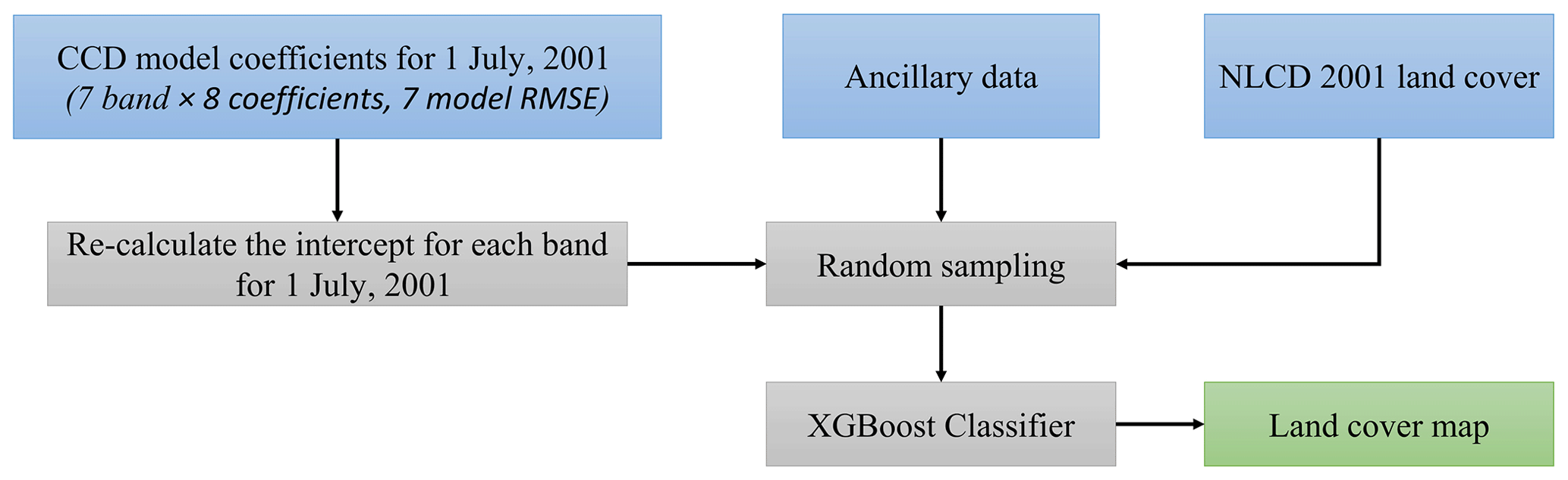
The CCDC algorithm characterizes the land cover component of a pixel at any point using the LCMAP time series model approach from the Landsat 4– Landsat 8 records. The classification of CCDC is accomplished for every pixel based on data from the time series models (e.g., model coefficients). Land cover classifications are generated on an annual basis, using 1 July as a representative date. A list of land cover classes and descriptions is provided in Table 1. Figure 3 illustrates an overall classification approach.

Figure 3 The overall approach of land cover classification in CCDC.

3.4.1 Classification algorithm

We chose eXtreme Gradient Boosting (XGBoost) (Chen and Guestrin, 2016) as the classification method. XGBoost is a scalable implementation of gradient tree boosting, which is a supervised learning method that can be used to develop a classification model when provided with an appropriate training dataset. Generally, for a given dataset, a tree ensemble model uses additive functions, which correspond to independent tree structures, to predict the land cover. The predictions from all trees are also normalized to the final class probabilities using the softmax function. The algorithm can handle sparse data and theoretically justify weighted quantile sketch for approximate learning. The resultant trained model can be applied to a larger dataset to generate predictions and probability scores which are the basis for LCMAP primary and secondary land cover types. The primary and secondary land cover confidence values are calculated from these scores.

3.4.2 Training dataset

The training data used in XGBoost for the LCMAP Collection 1.0 land cover products are from the USGS NLCD 2001 land cover product (Homer et al., 2020). To meet the LCMAP land cover legend, the NLCD data are first cross-walked to LCMAP classes, as shown in Fig. 4 and Table 2. The use of NLCD data that were cross-walked to the LCMAP land cover legend as the training data will reduce uncertainties and improve the consistency of annual land cover change. For example, grass and shrub have different ecological functions. Their spectral signatures are distinct in some ecological regions but are very close in others, especially in the western ecoregions of the conterminous United States (Underwood et al., 2007; Xian et al., 2013). Grass and shrub usually grow close together, making it difficult to separate them in thematic land cover. Combining these two cover classes can reduce uncertainties potentially caused by lack of spectral distinction in Landsat observations. Furthermore, the extent of each land cover class in the cross-walked NLCD layer is eroded by 1 pixel. This step aims to reduce potential noise in the classifier by removing pixels that may be heavily mixed with different cover types or whose land cover label may be less reliable. It also removes the narrow, linear, low-intensity developed pixels corresponding to road networks, which were found to have registration issues with Landsat ARD in some areas.

Figure 4 NLCD 2001 land cover (a), cross-walked LCMAP land cover classes (b), LCMAP land cover eroded by 1 pixel (c), zoomed-in cross-walked land cover from NLCD 2001 (d), and zoomed-in LCMAP land cover classes eroded by 1 pixel (e). The color legends represent the NLCD land cover class and LCMAP primary land cover (LCPRI).

Table 2 NLCD land cover cross-walked to LCMAP land cover.

3.4.3 Ancillary data

Ancillary data used in the classification contain two main datasets: the DEM and the WPI layer. Three DEM derivative datasets are implemented as geographic references for land cover classification as ancillary data including topographic slope, aspect, and position index. The WPI is highly related to wetland distribution and has potential to improve wetland classification in LCMAP.

3.4.4 Classification procedures

For each pixel, CCD segment data for the segment that includes the 1 July 2001 date are used with training data to create classification models (Zhou et al., 2020; Zhu et al., 2016). Data generated from the CCD models are used to make the land cover classification because different land cover classes can have different shapes for the estimated time series models. The coefficients of the CCD models including the overall mean and model coefficients except intercepts can be used to estimate the intra-annual changes caused by phenology and sun angle differences for the ith Landsat band. The information obtained from the time series model is useful for land cover classification. The CCD model data used with training data include the model coefficients (except the intercepts) generated from surface reflectance and brightness temperature bands, the model RMSE value for each band, and an average intercept value that is calculated from average annual reflectance values for each band for the 1 July 2001 year. The model training procedure is conducted at the tile level, using random samples drawn from the targeted tile as well as the eight surrounding tiles to avoid not having enough training samples of rare land cover types in the targeted tile. Cross-walked and eroded NLCD data are used for classification labels, while the CCD model outputs and ancillary data are provided as independent variables. Based on training data testing using different sample sizes, a target sample size of 20 million pixels from the extent of 3×3 ARD tiles is chosen, requiring approximately proportional representation of classes with the added constraint that no class be represented by fewer than 600 000 or more than 8 million samples. If there are fewer than 600 000 samples available for a class, then all of the available samples are used without any oversampling. The XGBoost hyperparameters are selected as maximum tree depth 8, the fast histogram optimized approximate greedy algorithm for the tree method, multiclass log loss for the evaluation metric, and maximum number of rounds 500.

After the classification models in a given tile are trained, predictions are generated for each 1 July date that has an associated CCD segment (Fig. 5). The prediction information is supplied to the production step for the creation of land cover. The process is repeated for each tile for the entire CONUS ARD extent.

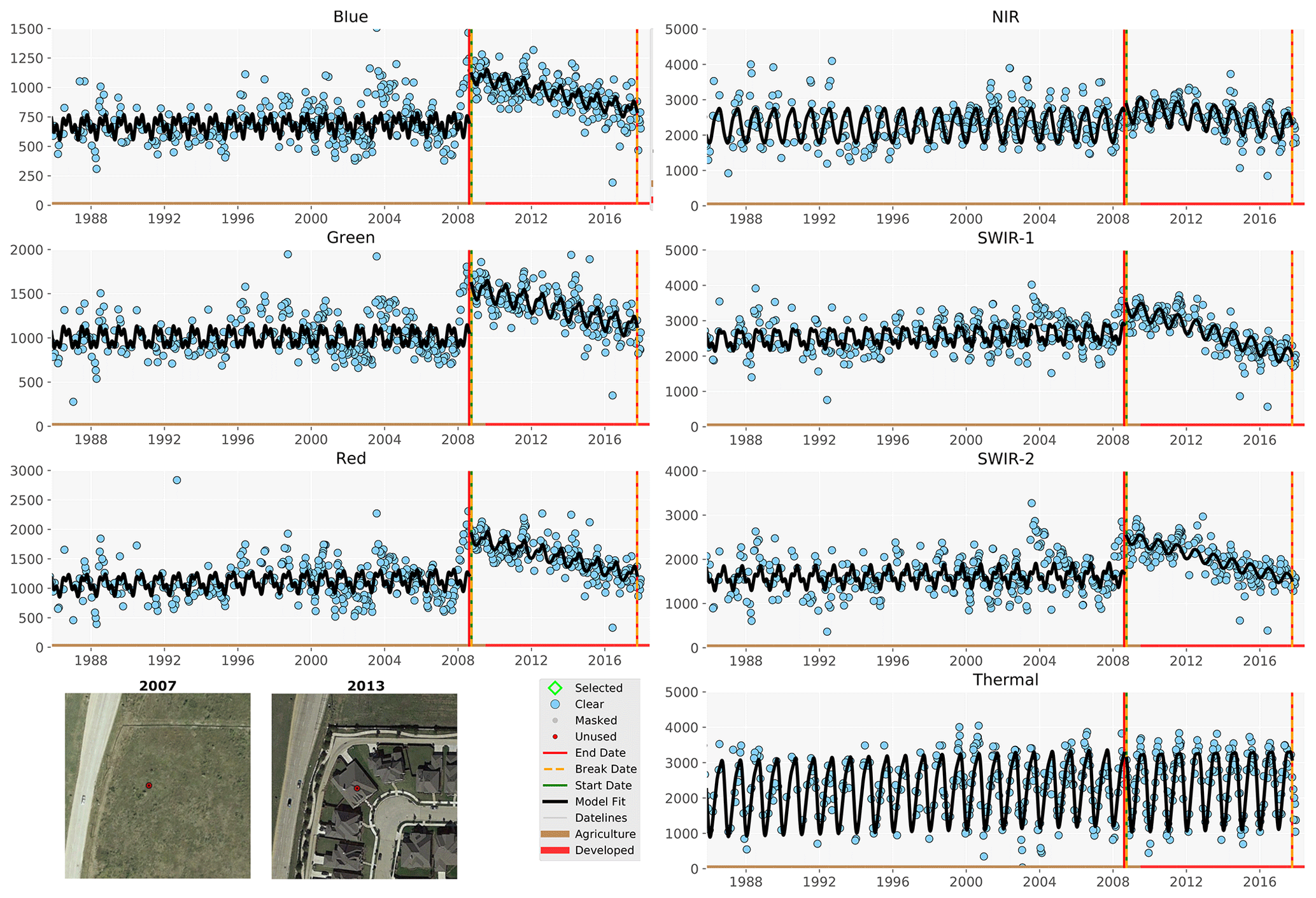
Figure 5 CCD change detection and segmentation using Landsat blue, green, red, near-infrared, shortwave infrared (SWIR) 1, shortwave infrared (SWIR) 2, and thermal bands. Blue dots are all available clear Landsat records in each year. The horizontal lines in different colors represent land cover classes labeled by the algorithm. The vertical lines show model break dates. The black line is the model fits. The high-resolution images show landscape conditions in 2007 and 2013.

3.5 Validation data

The LCMAP land cover product is validated using an independent reference dataset. The reference data, which consist of 24 971 pixels of 30 m × 30 m selected via a simple random sampling method over CONUS, are collected from these sample plots between 1985 and 2017. The TimeSync tool is used to efficiently display Landsat data for interpretation and to record these interpretations into a database (Cohen et al., 2010; Pengra et al., 2020b; Stehman et al., 2021). TimeSync displays the input Landsat images in two basic ways: by annual time series images and by pixel values plotted through time. For the image display, single 255×255-pixel subsets of Landsat images in the growing season are displayed in sequence from 1984 to 2018. Trained interpreters have access to all available images in each year to collect attributes in three basic categories: (1) land use, (2) land cover, and (3) change processes. Additional attribute details for the change processes, such as clear-cut and thinning associated with harvest events, are also collected. The interpreters manually label these attributes using Landsat 5, Landsat 7, and Landsat 8 imagery; high-resolution aerial photography; and other ancillary datasets (Cohen et al., 2010; Pengra et al., 2020b). Interpreters also use ancillary data to support interpretation of Landsat and high-resolution imagery, although Landsat data take the highest weight of evidence. Recording the full set of attributes in land use, land cover, and land change categories provides sufficient information to meet the needs of LCMAP as well as those of other potential users. Quality assurance and quality control (QA–QC) processes are also implemented to ensure the quality and consistency of the reference data among interpreters and over the time span of data collection (Pengra et al., 2020b). Each reference sample is interpreted by a trained interpreter, and about 60 % of these pixels are interpreted independently by a second analyst. Much of the QA–QC process relies on comparing the interpretations at these duplicated sample pixels. Duplicated sample pixels that have interpreter disagreement are evaluated in the QA–QC process, focusing on identifying issues with specific classes or interpreters, flagging sample pixels for further review and possible editing, and providing ongoing training and feedback to interpreters throughout the collection process. QA–QC-related reviews are also completed on sample pixels that show interpretation data such as uncommon and/or illogical land use and land cover combinations, multi-year disturbance processes, rare classes, or other opportunistically identified situations. Interpreted attributes of sample pixels are edited, if necessary, to create the final attribute assignments for the reference data. These final attributes are then cross-walked to a single LCMAP land cover class label, providing a single land cover reference label for each year of the time series for each sample pixel.

The validation analysis protocols focus on estimating the confusion matrix and overall, user's, and producer's accuracy by comparing the reference data and product data labels. Overall accuracy and producer's accuracy as well as standard errors are produced using post-stratified estimators (Card, 1982; Stehman, 2013). For accuracy estimates that are produced by combining multiple years of data, the sampling design is treated as a one-stage cluster sample where each pixel represents a cluster and each year of observation is the secondary sampling unit using cluster sampling standard error formulas (Pengra et al., 2020b; Stehman et al., 2021). The validation is only performed for primary land cover and change products, not for other LCMAP science products (Sect. S4 in the Supplement).

3.6 Information warehouse and data store

LCMAP adopts an information warehouse and data store (IW+DS) system that can expand storage solutions along with data access and discovery services running on the EROS shared Mesos cluster. The system provides different storage solutions to allow for flexibility in choosing what best fits a dataset's characteristics and currently comprises Apache Cassandra (https://cassandra.apache.org/_/index.html, last access: 30 November 2021) and Ceph (https://ceph.io/en/, last access: 30 November 2021) object storage. The services provide data ingest, retrieval, discovery, metadata, processing, and other functionalities. LCMAP maintains a copy of Landsat Collection 1 ARD and other similarly tiled ancillary datasets that are spatially subset within the IW+DS to allow efficient retrieval and to enable large-scale CCDC processing and other algorithmic work. The ingest process is designed to avoid bringing in ARD tile observations that are already present within the IW+DS, to keep the input consistent with any prior usage while allowing CCDC to bring in new observations as they are available. Algorithmic results, products, and other intermediate data are kept in the Ceph object store arranged using a prefix structure to label the identity of the data, with the actual object names incorporating spatial concepts such as tile and chip, which is a small subset of a tile and contains 100×100 pixels of 30 m.

4 Results and discussion

The LCMAP primary land cover and change products were evaluated to outline annual land cover change from 1985 to 2017 in the conterminous Unites States.

4.1 Collection 1.0 primary land cover distribution and change

The CONUS primary land cover mapping result and the primary confidence in 2010 are shown in Fig. 6a and b, respectively. The land cover map illustrates distributions of different land cover types across CONUS. The primary confidence is above 90 % for most land cover classes, suggesting that the classification models were created with high confidence for land cover mapping for most classes in most regions. Some vegetation transition (green in Fig. 6b) occurs mainly in the southeast region, suggesting gradual tree recovery from disturbances associated with tree harvesting. Figure 6c and d display numbers of land cover changes and spectral changes detected by the CCDC model between 1985 and 2017. The number of land cover changes represents how many times land cover has changed from one type to another for a specific pixel. However, the number of spectral changes denotes how many times the model has detected spectral changes in a CCD time series model where spectral observations have diverged from the model predictions. These changes could relate to a change in thematic land cover or might represent more subtle conditional surface changes. The southeast region shows more frequent land cover changes in the 33 years (Fig. 6c). The western part of CONUS, however, contains more spectral changes than in the east (Fig. 6d). The NLCD land change estimates also show similar change patterns between 2001 and 2016 (Homer et al., 2020). The different spatial patterns in the total number of land cover changes (Fig. 6c) and detected spectral changes (Fig. 6d) suggest that not all changes lead to land cover change (e.g., drought and precipitation-related changes in vegetation or grassland fire). The large numbers of spectral change were mainly detected in the southern grassland area.

Figure 6 Illustration of the LCMAP product: (a) primary land cover in 2010, (b) primary land cover confidence in 2010, (c) the frequency of land cover changes from 1985 to 2017, and (d) the total number of spectral changes detected from 1985 to 2017.

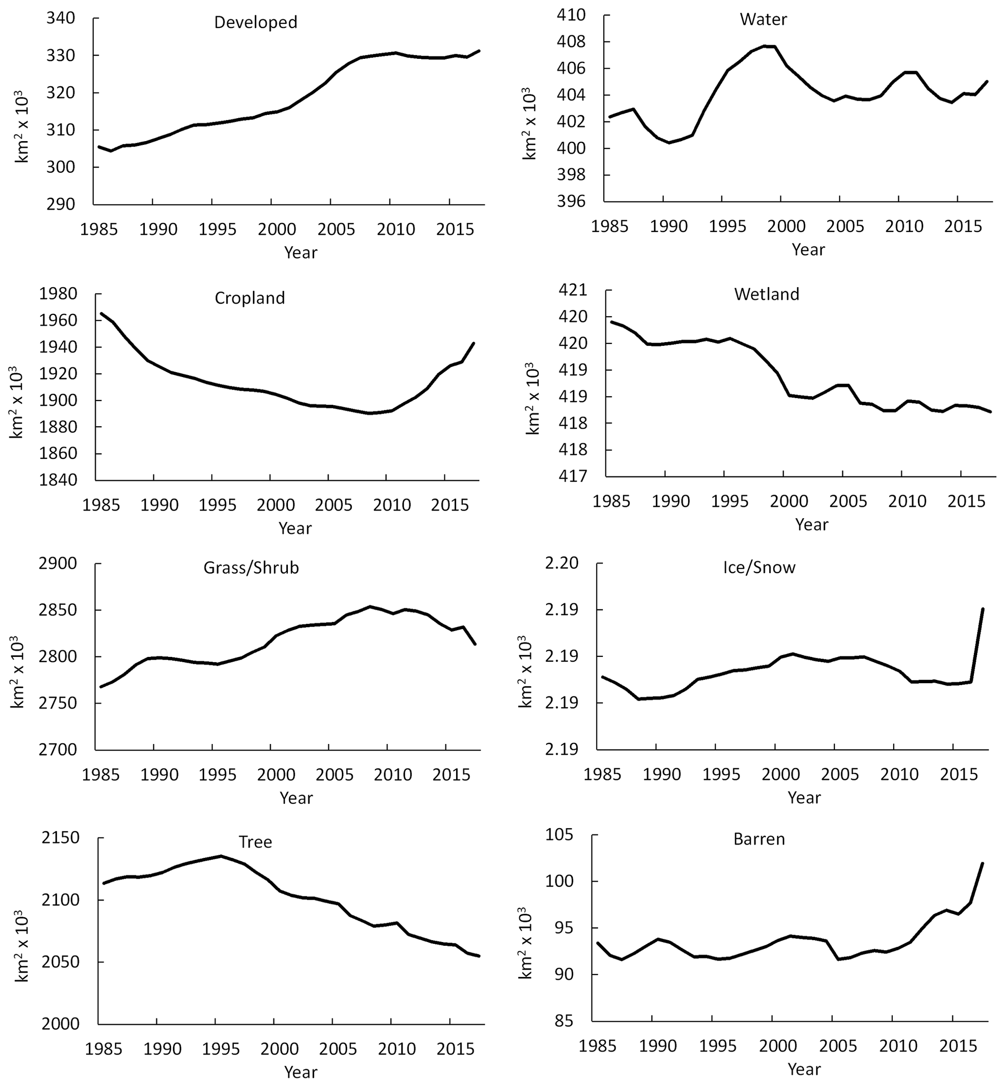
Figure 7 shows the temporal changes of areas for eight land cover classes from 1985 to 2017. Among all classes, grass/shrub, tree cover, and cropland were dominant land cover types, followed by wetland, water, developed, barren, and snow/ice. The land cover and change datasets show that developed land has a consistent increasing trend with an 8.4 % increase while barren increased 9.1 % between 1985 and 2017. Overall, the developed and barren areas increased 2.58×10⁴ and 8.56×10³ km², respectively. Other land cover categories do not have such increasing patterns. As for water, although fluctuating, it had a generally increasing trend. The area of wetland had a rapid decrease before 2000, following a relatively steady though fluctuating trend. Net wetland extent declined about 0.4 % from 1985 to 2017. The grass/shrub and tree cover classes both experienced consistent increasing trends before 2008 and 1995, respectively, with areas reaching about 2.85×10⁶ km² for grass/shrub and 2.14×10⁶ km² for tree in these 2 years. These two land covers have gradually decreased since then. Tree cover declined after 1996, showing a decreasing rate of 2.8 % between 1985 and 2017. The cropland decreased from 1985 to 2008 and quickly increased after that. By 2017, the area of cropland had reached a similar level of cropland area to that in 1988. Furthermore, most land cover changes are located in the southeast region where many pixels change more than one time. The changes detected by the CCD model suggest that landscape in the Midwest and west are more dynamic than in the east. Many areas experience multiple disturbances although most of these changes do not result in land cover transition.

Figure 7 Areal variations in eight primary land cover types from 1985 to 2017 in CONUS.

The south ARD tile outlined in Fig. 6a covers the northern Dallas region, and the spatial patterns of land cover and change are shown in more detail in Fig. 8. The land cover distributions in the region show that urban land expanded considerably from 1985 (Fig. 8a) to 1990 (Fig. 8b) and to 2016 (Fig. 8c). The land conversion was primarily from cropland and grass/shrub to developed land. Lake Ray Roberts was created in the late 1980s and captured in the land cover map (Fig. 8b and c). The lake and urban conversion are also visible in the change count from 1985 to 2016 (Fig. 8g), which mainly shows as blue, suggesting a one-time conversion. On the other hand, there is almost no change in the urban center (Fig. 8g). Figure 8d–f show high classification confidence at the urban center, water, grass/shrub, and tree cover areas, whereas cropland is associated with relatively low confidence, indicating frequent management activities over croplands in the regions. The total pixels of different change numbers suggests that one to two change times are dominant, although some pixels change more than three times (Fig. 8h). The land cover distributions in 1985, 1990, and 2017 show an increase in developed land and decreases in cropland and grass/shrub (Fig. 8i).

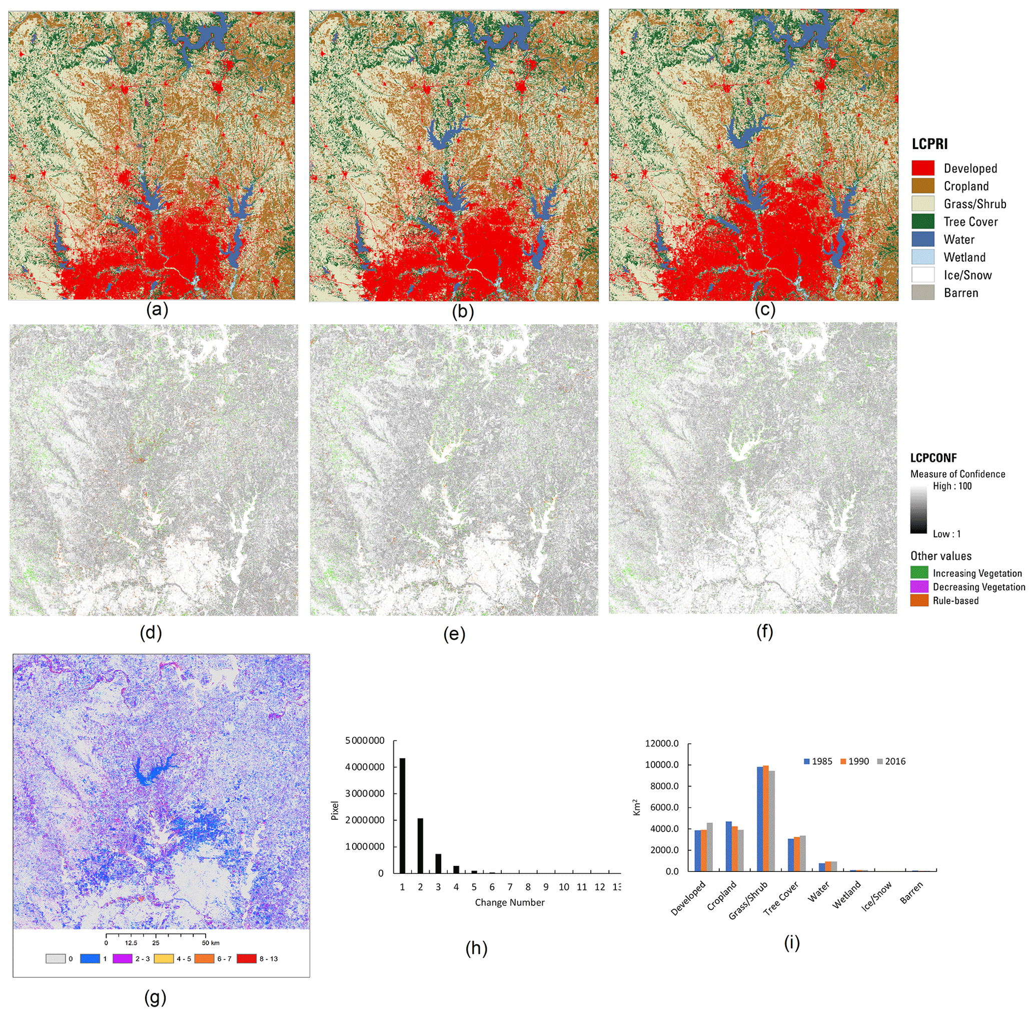
Figure 8 Primary land cover and confidence in 1985 (a, d), 1990 (b, e), and 2016 (c, f) and change in 1985–2017 (g), the frequency of land cover change (x axis) from 1985 to 2017 and numbers of pixels (y axis) of these changes (h), and areas (y axis) of different land cover (x axis) in the three times for the ARD tile 16_14 (i).

The spatial patterns of land cover and change in the north ARD tile displayed in Fig. 6a in northern Wyoming are shown in Fig. 9. The tile covers most of Yellowstone National Park, in which tree, grass/shrub, and water are three dominant land cover types. Land cover in 1985, 1990, and 2016 (Fig. 9a–c) changed from tree to grass/shrub and back to tree cover. The primary land cover confidence layers exhibit changes as decreasing vegetation from tree to grass/shrub and increasing vegetation from grass/shrub to tree (Fig. 9d–f). For those trees and water bodies that did not experience any disturbances, their magnitudes of confidence are relatively large. The change map suggests that most forest lands experienced at least one change and some areas changed multiple times (Fig. 9g). Most changes in forest lands were related to wildland fires that occurred in the region. In 1988, 50 fires burned a mosaic covering nearly 3213 km² in Yellowstone as a result of extremely warm, dry, and windy weather (NPS, 2021). Trees regrew in some of the burn areas, and these changes could occur more than once as shown in the change map, which indicates at least two changes in these areas. The total pixels of different change frequencies suggests that one to two changes were dominant and very few pixels changed more than three times (Fig. 9h). The land cover distributions in 1985, 1990, and 2017 had increases in grass/shrub after 1985 and reductions in tree cover after that (Fig. 9i).

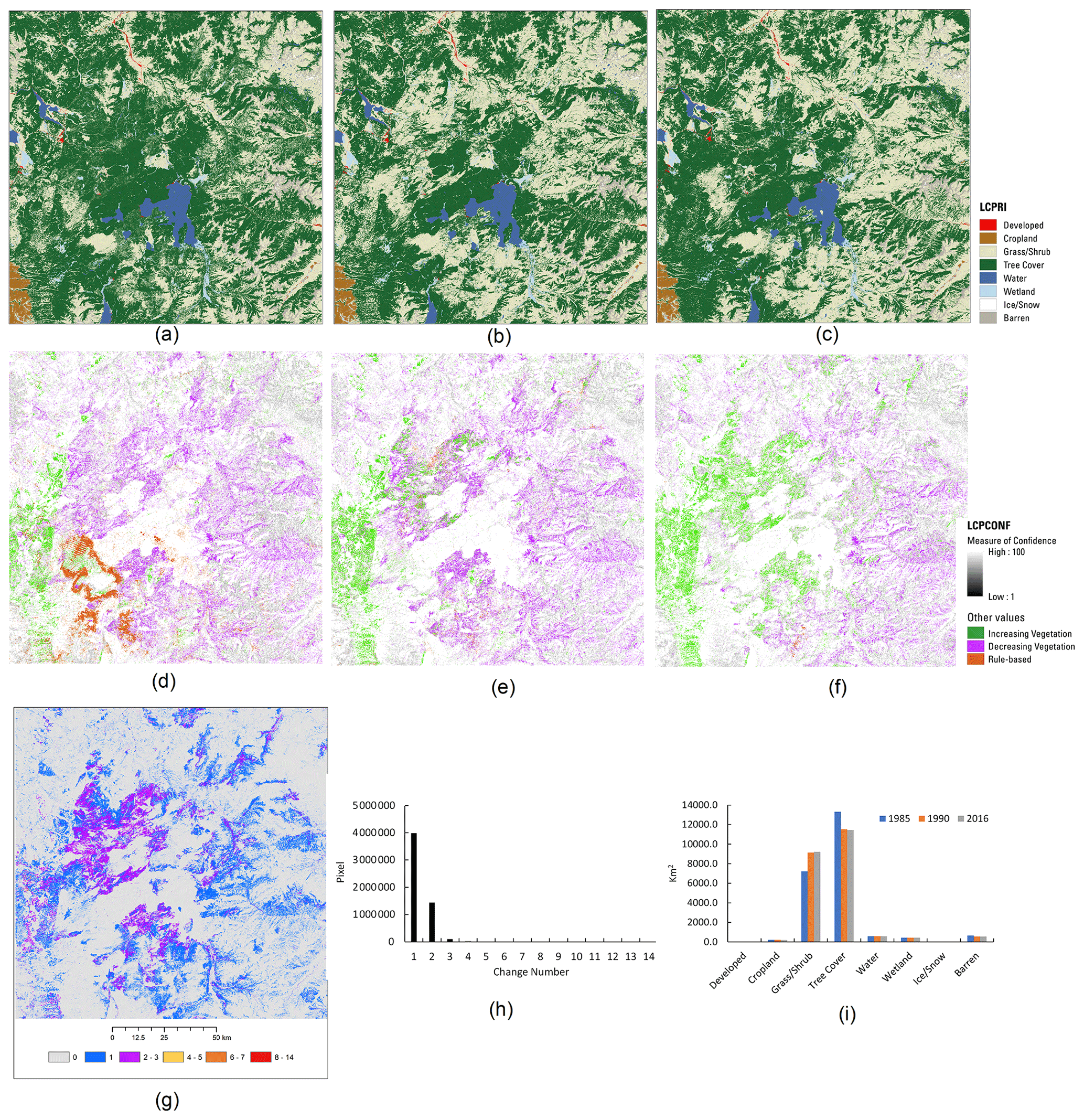
Figure 9 Primary land cover and confidences in 1985 (a, d), 1990 (b, e), and 2016 (c, f) and change in 1985–2017 (g), the frequency of land cover change (x axis) from 1985 to 2017 and numbers of pixels (y axis) of these changes (h), and areas (y axis) of different land cover (x axis) in the three times for the ARD tile 9_6 (i).

4.2 Validation of land cover product

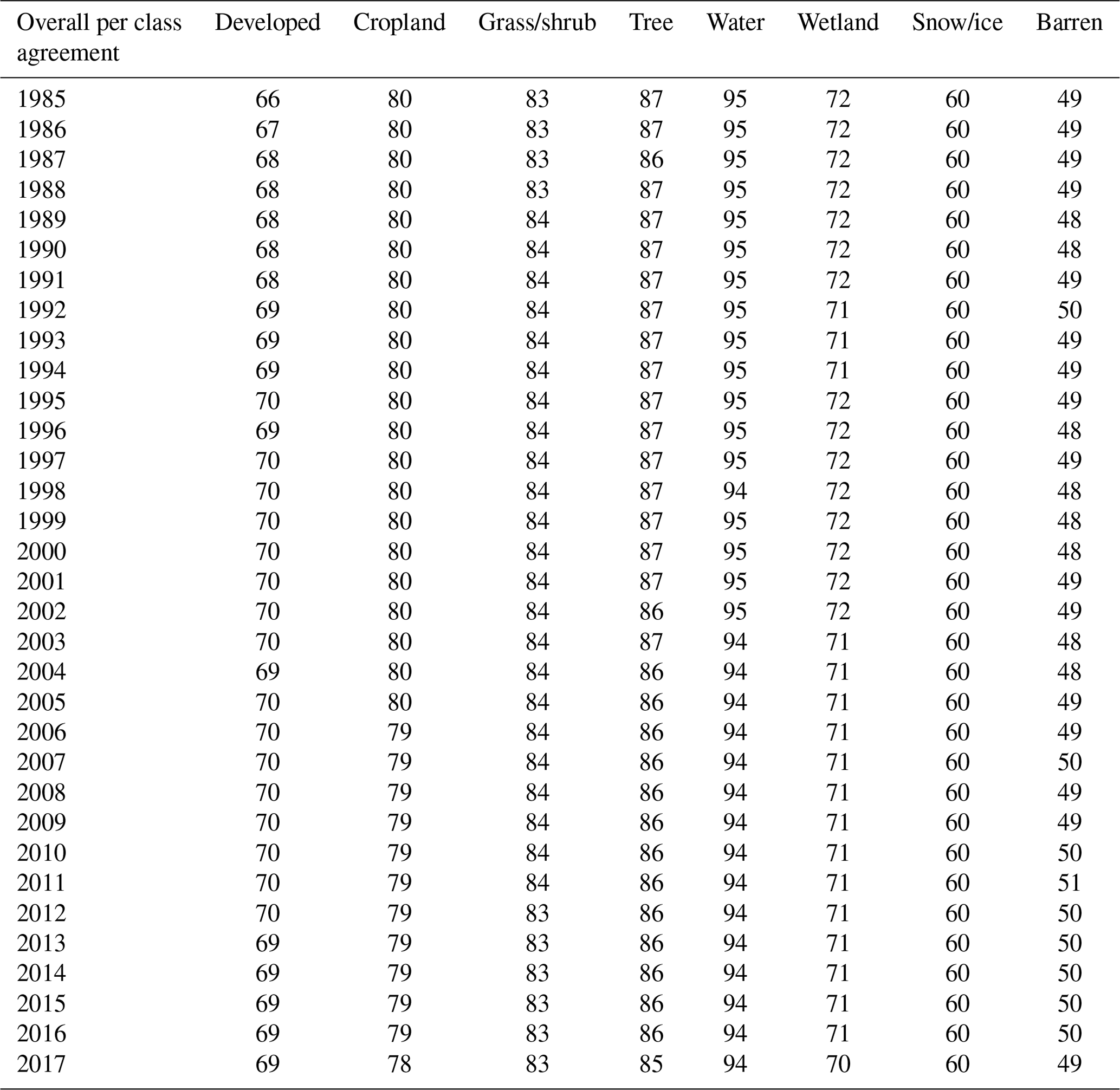
The overall accuracy between the annual reference land cover label and the LCMAP annual land cover products was calculated as 82.5 % (±0.22 %, standard error) when summarized for all years. Overall accuracy across the time series (1985–2017) varied within about 1.5 % annually, ranging from a high of 83 % in the late 1990s to about 82 % in the late 2010s (Fig. 10). Per class accuracies across CONUS ranged between 43 % and 96 % for user's accuracy (Table 3), with water showing the highest accuracy (96±0.5 % user's accuracy and 93±0.7 % producer's accuracy). Cropland has about 93 % (±0.3 %) producer's accuracy and 70 % (±0.6 %) user's accuracy. The lowest accuracies are observed for barren and wetland. The per class per year agreements show the accuracies vary slightly for each class in each year (Table 4). The variations in annual overall accuracy are within a range of about 1.5 % across the time series. The slight decline in annual overall accuracy suggests that year-to-year trends may be a result of a complex interplay of temporal biases in the LCMAP algorithm, Landsat data quality and quantity, the model break detection accuracy of the LCMAP CCD, and errors in the training data used for the classification. For example, the change detection portion of the algorithm is known to be conservative in identifying land cover change. The CCD model assumes that the spectral variations in the land surface through time can be characterized with annual harmonic models and can be separated into discrete periods of time. Therefore, the model performs better when the short-term spectral variability of the land surface is low, the changes have a large spectral response, and the observational data density is high. Over time, the actual land cover may evolve away from the phenology represented by spectral models that may have missed one or more spectral breaks, which will impact accuracy especially when the land cover changes are persistent rather than cyclic, such as with an expanding urban footprint. Annual accuracy of developed showed an upward trend in user's accuracy (UA) and a downward trend in producer's accuracy (PA) over time (Stehman et al., 2021). The increasing availability of high-resolution data used by the interpreters may have increased the likelihood of identifying features characteristic of developed land that could not be identified earlier in the time series, leading to an increase in the proportion of developed area estimated from the sample. Consequently, the increasing sensitivity of the reference interpretation to landscape features may account for the difference between the mapping and the reference data over time. Lower data density toward the beginning and end of the time series may decrease accuracy, which when combined with other factors, can contribute to the annual land cover overall accuracy across all years.

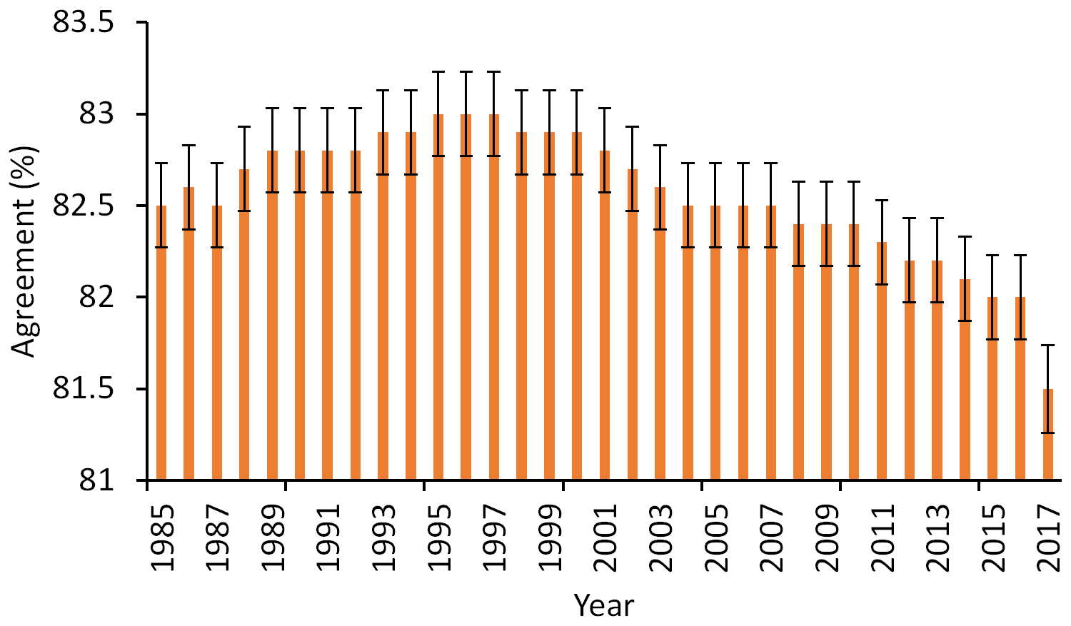
Figure 10 Overall agreement between LCMAP primary land cover and reference data across CONUS. The black error bars represent ±1 standard errors.

Table 3 Confusion matrix for CONUS (all years combined) where cell entries represent percent of CONUS area. Overall accuracy is 82.5 % (±0.22 %). Standard errors for user's and producer's accuracies are shown in parentheses and n is the number of sample pixels for each row and column.

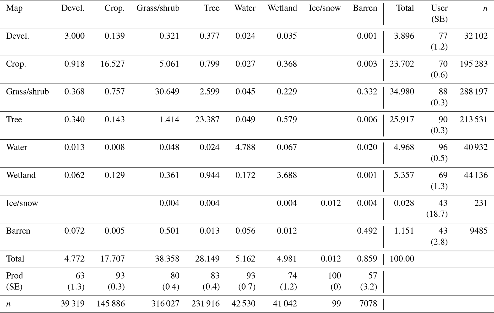
Table 4 Overall per class agreement as percentages between 1985 and 2017.

4.3 Significance of the product

One of the biggest advances of LCMAP relative to conventional methods available to date is its approach of generating annual land change products by using the entire Landsat archive at a large geographic scale. Landsat ARD, which is the foundation for LCMAP, is effective and straightforward for tracking and characterizing the historical land changes at a pixel level over decades. Compared to conventional methods, detecting changes using all available observations enables us to date these changes as they occur. After change is detected, temporally consistent land cover products rather than stochastic changes in labels can be produced at annual intervals by conducting classification from CCD model segmented contributions.

The LCMAP product suite includes five land cover change and five land surface change science products. It represents a new paradigm that consistently and continuously provides a large volume of land change information for land change monitoring, land resource management, and scientific research. In addition to primary and secondary land cover before and after changes, change segments containing spectral change time and magnitude are provided to explore the changes in land condition and could meet various user communities' needs. The LCMAP products can improve our understanding of the causes, rates, and consequences of the land surface changes such as forest changes caused by wildfire and insect outbreaks.

By implementing the CCDC algorithm through a system engineering approach, LCMAP provides a fully automated framework for land change monitoring. The framework can also be updated to include the latest Landsat records so that it can be used for operational continuous monitoring in a large geographic extent (Brown et al., 2020). Therefore, when new observations become available, the framework can provide timely and consistent land cover characteristics to the public.

4.4 Limitations and challenges

Although LCMAP Collection 1.0 products have been proven to be successful in detecting various land surface changes to support research applications related to environment and ecology conditions, limitations and challenges exist. Utilizing Landsat ARD data as input provided consistent time series Landsat imagery with high-level geometric and radiometric quality for implementing the CCDC method. Nevertheless, the densities of Landsat observation records varied greatly across space and time due to spatial differences in Landsat scene overlap and temporal coverage, as well as regional differences in contamination by clouds, cloud shadows, and snow. The change detection accuracies of CCD models were highly influenced by the temporal frequency of available observations. Zhou et al. (2019) found that using harmonized Landsat 8 and Sentinel-2 data increased the temporal frequency of the data and thus enhanced the ability to model seasonal variation and derived better change detection results than using Landsat data alone. Integrating multi-mission data could provide the opportunity to enhance change detection, especially for the land cover types that are highly dynamic or in frequently cloudy/snowy areas.

Providing only eight general land cover classes and their changes in LCMAP Collection 1.0 products limits the usage of the product in some applications that need a higher level of thematic land cover detail. For example, shrub and grass are two major vegetation types and have different ecological functions, but they are not delineated separately in LCMAP Collection 1.0 products. Lack of measurement of grassland–shrub transition constrains the study of shrub encroachment, which is a symptom of land degradation. However, the NLCD 2001 level I land cover product had different mapping accuracies for different land cover types in different ecological regions (Wickham et al., 2010). For example, the grass mapping accuracies were higher in the eastern regions than they were in most western mapping regions. The accuracies of shrub cover had similar variation patterns across CONUS. These accuracy variations suggest uncertainties in the products, especially in most western regions where grass and shrub are more difficult to separate. Combining grass and shrub from the NLCD 2001 product reduced uncertainties introduced by the two individual components and made the accuracy of the grass/shrub product in LCMAP relatively high and consistent across CONUS (Stehman et al., 2021). NLCD has established new efforts to improve mapping accuracies by adding innovative approaches for land cover classification and introducing continuous rangeland products in western CONUS for NLCD thematic land cover products since 2001 (Homer et al., 2020). The use of new NLCD products as the training data will support LCMAP to produce more land cover types including separating grass and shrub in the future.

Adopting the NLCD land cover product as the training data source efficiently provided abundant training samples to deliver a land cover product with high classification accuracy. Selecting a sufficient size of training samples is important for CCDC models to obtain accurate classification. Previous land cover post-classification analysis suggested that the overall classification accuracy increased when the training samples increased (Gong et al., 2020). The recent global land cover classification also suggested that the appropriate training sample size for a mapping extent of three 158 km × 158 km tiles should be larger than 60 000 (Zhang et al., 2021). For the LCMAP land cover classification, a much larger training size was utilized to ensure that these training samples could represent landscape features in the classification tiles. However, these training data were randomly selected from the NLCD land cover product, suggesting errors could potentially be carried over to the training samples due to potential errors in the training source. Besides uncertainties in training data, some obvious challenges such as class definitional differences between pasture/hay and grassland between NLCD and LCMAP could potentially be carried over to the LCMAP land cover product. Implementing training data by reducing uncertainties and potential errors in a more consistent and accurate way is critical to strengthen land cover classification and to improve the scientific quality of LCMAP products in the future.

There are apparent shifts in some land cover types, especially in snow/ice and barren (Fig. 7), and a decline in overall agreement (Fig. 10) in 2017, the last year of the Collection 1.0 product. The last year's product is usually provisional because limited Landsat observations are available at the end of a time series. The CCDC requires at least 24 clear observations to create full models for change detection and classification. Without sufficient clear observations, the algorithm could not produce model breaks accurately. Therefore, in the last year of a time series, the rule-based assignment is implemented to label land cover for these pixels that do not have enough observations to build a time series model. Both primary and secondary land cover classes are assigned from the last identified primary and secondary classes.

5 Data availability

The LCMAP products generated in this paper are available at https://earthexplorer.usgs.gov/ (last access: 30 November 2021). All LCMAP land change products are mosaicked for the conterminous United States in the GeoTIFF format. Find exact data as described here at https://doi.org/10.5066/P9W1TO6E (LCMAP, 2021). The reference dataset used for the product validation is also available at https://doi.org/10.5066/P98EC5XR (Pengra et al., 2020a).

6 Conclusions

The continuous Landsat observations spanning from the 1980s to the present, new generations of change detection and classification models, and systems capable of processing large-volume data are offering unprecedented opportunities to characterize land cover and detect land surface change consistently and accurately. Additionally, the collection of reference data used to validate land cover products provides validation results for each land cover category annually. To capture the variability in landscape condition and its responses to different disturbances, land cover and land surface change datasets need to be produced over a large geographic scale. LCMAP has produced a suite of land change products at a 30 m resolution including the reference dataset in the United States. In that context, LCMAP was developed to generate an essential dataset to meet broad scientific research and resource management needs. Using the CCDC algorithm and Landsat ARD to determine whether change has occurred at any given point in the observation record, LCMAP produced annual land cover and change datasets for the conterminous United States in a robust manner. These new datasets and the novel production systems will allow for a new generation of research and applications in connecting time series remote sensing observations with land surface change at a much finer scale than previously possible.