EstSoil-EH: a high-resolution eco-hydrological modelling parameters dataset for Estonia

To understand, model, and predict landscape evolution, ecosystem services, and hydrological processes, the availability of detailed observation-based soil data is extremely valuable. For the EstSoil-EH dataset, we synthesized more than 20 eco-hydrological variables on soil, topography, and land use for Estonia (https://doi.org/10.5281/zenodo.3473289, Kmoch et al., 2019a) as numerical and categorical values from the original Soil Map of Estonia, the Estonian 5 m lidar DEM, Estonian Topographic Database, and EU-SoilHydroGrids layers.

The Soil Map of Estonia maps more than 750 000 soil units throughout Estonia at a scale of 1:10 000 and forms the basis for EstSoil-EH. It is the most detailed and information-rich dataset for soils in Estonia, with 75 % of mapped units smaller than 4.0 ha, based on Soviet-era field mapping. For each soil unit, it describes the soil type (i.e. soil reference group), soil texture, and layer information with a composite text code, which comprises not only the actual texture class, but also classifiers for rock content, peat soils, distinct compositional layers, and their depths. To use these as eco-hydrological process properties in modelling applications we translated the text codes into numbers. The derived parameters include soil layering, soil texture (clay, silt, and sand contents), coarse fragments, and rock content of the soil layers within the soil profiles. In addition, we aggregated and predicted physical variables related to water and carbon cycles (bulk density, hydraulic conductivity, organic carbon content, available water capacity).

The methodology and dataset developed will be an important resource for the Baltic region, but possibly also for all other regions where detailed field-based soil mapping data are available. Countries like Lithuania and Latvia have similar historical soil records from the Soviet era that could be turned into value-added datasets such as the one we developed for Estonia.

1 Introduction

Soil has remarkable complexity and through its various functions plays a key role in Earth's ecosystems. It provides multiple ecosystem services to humans, such as food and clean water. Recent studies have highlighted the role of properly functioning soils that can provide their ecosystem services for the achievement of the United Nations (UN) Sustainable Development Goals (SDGs) (Keesstra et al., 2018, 2016). Therefore an accurate quantitative description and prediction of soil processes and properties is essential in understanding the impacts of climate and land use changes on ecosystem services (Van Looy et al., 2017). For this purpose, spatially accurate maps of soil properties are needed where detailed soil survey data are available. But unfortunately, these are either missing for many countries and regions in the world or exist with insufficiently fine spatial resolution (Nussbaum et al., 2018). However, for many countries field-based data on soil properties are still available. Moreover, the recent increase in spatial environmental data created by remote sensing (climatic, terrain variables etc.) can be used for deriving the desired soil properties at fine resolution. There are several useful approaches to combine, or fuse, several datasets into one and obtain the complete spatial coverage of the soil properties needed for modelling.

At the global level, two main soil databases are available. The first was made available by the United Nations Food and Agricultural Organization (FAO): the Harmonized World Soil Database (HWSD) v1.2 (Fischer et al., 2008). The dataset is a 30 arcsec raster database (approx. 100 ha resolution) with more than 15 000 different soil mapping units. It combines existing regional and national updates of soil information from around the world. Another global-level soil database is SoilGrids250m (Hengl et al., 2017), which provides harmonized gridded soil data with values for sand, silt, clay, and rock fractions, as well as organic carbon and carbon stocks at several depths with a resolution of approx. 6.5 ha which can be used as inputs for eco-hydrological models, e.g. SWAT (Abbaspour et al., 2019). SoilGrids250m has been derived with machine-learning methods using environmental variables, such as terrain properties, as predictor variables and field-based soil profiles as the training set (Hengl et al., 2017). This approach takes advantage of the recent abundance of high-resolution environmental spatial data mostly obtained from remote sensing (e.g. terrain, climatic variables, soil moisture) and employs these datasets as explanatory variables to model soil properties at fine spatial resolution (Nussbaum et al., 2018). Analogously, EU-SoilHydroGrids (Tóth et al., 2017) provides a 3D soil hydraulic database for Europe (available in 250 m and 1 km resolution) based on SoilGrids250m and trained pedotransfer functions (PTFs). In other words, they use machine-learning regression as specialized PTFs.

PTFs are predictive functions of certain soil properties, such as organic carbon content or bulk density, using data from field-based soil surveys (e.g. sand, silt, and clay content). However, the potential of available PTFs has not been fully exploited and integrated into eco-hydrological modelling and ecosystem services provided by soils (Van Looy et al., 2017). For example, soil organic carbon (SOC) is an important indicator of soil health and plays a key role in the global carbon cycle, and therefore it is crucial to adequately quantify and monitor SOC changes (Vitharana et al., 2017). However, reliable estimates for SOC have been difficult to obtain due to a lack of measured soil profile data to train the model (Eswaran et al., 1993). Very few SOC datasets are available for many countries or regions. For example, the Northern Circumpolar Soil Carbon Database (Tarnocai et al., 2009) was developed to describe the SOC pools in soils of the northern circumpolar permafrost region. SOC stocks were also predicted under future climate and land cover change scenarios using a geostatistical model for predicting current and future SOC in Europe (Yigini and Panagos, 2016). Prévost (2004) described predictions of soil properties from the SOC content and found that SOC was closely related to soil bulk density (BD) and porosity. Suuster et al. (2011) emphasized the importance of BD as an indicator of soil quality, site productivity, and soil compaction and proposed a PTF for the organic horizon in the arable soils in Estonia. Abdelbaki (2018) evaluated the predictive accuracy of 48 published PTFs for predicting BD using State Soil Geographic (STATSGO) and Soil Survey Geographic (SSURGO) soil databases from the United States.

However, these regional datasets are often not detailed enough for country-level applications nor do they benefit fully from local high-resolution field-based soil data, as is the case for Estonia. There is no national-scale dataset of measurements or predictions of SOC or BD for Estonia, and no large-scale high-resolution soil database is currently available with numerical data for a range of typical eco-hydrological process-based models or to monitor SOC changes. However, Estonia has a national highly detailed digitized soil map (1:10 000) with 75 % of mapped units smaller than 4 ha. It was created based on extensive field mapping during the Soviet-era and can serve as an excellent basis for PTFs and robust models to predict soil properties at any given location (Minasny and Hartemink, 2011).

The objective of the present study was to develop a numerical soil database, EstSoil-EH, for modelling and for predicting eco-hydrological processes in Estonia and to provide a solid basis to estimate ecosystem services. The foundation of EstSoil-EH is the Soil Map of Estonia, which includes information about soil type, layering of the soil profile, textures (clay, silt, and sand content), coarse fragments, and rock content. We derived numerical values for the key characteristics for the whole of Estonia. High-resolution environmental data available nowadays allow improved PTFs and modern advanced methods (e.g. machine learning, geostatistics) for extrapolation and upscaling to be developed (Gunarathna et al., 2019; Van Looy et al., 2017). We employed machine learning and PTFs to derive and aggregate additional soil variables related to the water and carbon cycle based on high-resolution field-survey soil data and other environmental covariates (e.g. terrain variables).

2 Materials and methods

2.1 Background on the Soil Map of Estonia

We performed extensive database standardization on the original Soil Map of Estonia as the working basis and synthesize all further variables based on the standardized dataset sequentially. Figure 1 illustrates the major working packages and their inputs and outputs of eco-hydrological parameters.

The base dataset – the original Soil Map of Estonia – is based on observed data (e.g. texture, soil profile depth, rockiness, presence of organic layer). Systematic mapping of Estonian soils to produce a paper-based soil map at scales of 1:5000 and 1:10 000 was started in 1954 (Reintam et al., 2005), with most intensive field surveys in the period 1965–1969, for the main purposes of land evaluation and assessing potential for agricultural use. Generally, field mapping was carried out at a scale of 1:10 000 but in hilly or undulating areas with higher soil diversity at a scale of 1:5000, which resulted in mapped units with areas as small as 2500 m². During 1982–1988 older mapping data were updated and new areas were included with full-area soil quality assessment (primarily fertility, rockiness, water regime, texture, erodability). During 1988–1990 soil field surveys were performed for non-arable lands and ameliorated lands. Forest soils were mapped during 1976–1989. During these large-scale field-mapping activities, soil texture was determined in situ based on organoleptic methods (feel methods), and for reference profiles laboratory analyses were performed. This enabled calibration between texture defined by the organoleptic method by each researcher participating in field survey and texture determined in the laboratory (Estonian Landboard, 2017).

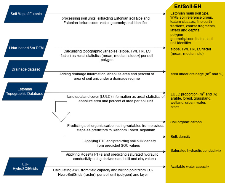
Figure 1 Flowchart for executed processing steps outlining the work packages, input datasets, and derived eco-hydrological modelling parameters on soil, topography, and land use.

As the result of large-scale soil mapping, 119 soil varieties have been distinguished in the Estonian national classification system and more than 500 combinations of texture type description have been collated. About 10 000 profiles up to 1 m depth (1 profile per 330 ha) have been sampled and analysed for characterization of mineral soils (Reintam et al., 2003, 2005). Thus, the texture codes and soil types assigned to the ca. 750 000 mapped soil units (polygons) are based on many decades of in situ land surveying practices.

Between 1997 and 2001, the soil map was digitized and attribute data were inserted into the database, resulting in the official National Soil Map of Estonia, a GIS vector dataset containing 750 000 soil units. It is available from the Estonian Land Board in several formats under a permissive open data license (Estonian Landboard, 2017). A copy with the original shapefile dataset, the related required documentation, and checksums has been archived for reference (Estonian Landboard, 2017).

The Estonian soil map contains the following attribute fields:

• Soil type. A designation of the soil name, the Estonian analogue to the World Reference Base (WRB) soil reference groups;

• Texture. A combination of texture classes defined for fine and coarse fragments, and to which depths the same texture and coarse fragments are observed (layer).

These attributes are encoded as “string” values, which include both letters and numbers. The important fields soil type and texture are not just stored as standardized class values but are instead a coded description based on abbreviations that are then combined with numbers for example depths and indicators for the level of erosion and are grouped together for different depths within the same attribute field. These description-based attribute values make it difficult to derive the foundational numerical values for sand, silt, clay, and coarse fragments from the codes and to make them more consistent and usable in calculations and statistical analyses.

2.2 Extraction of texture classes and soil reference groups and deriving basic physical and textural values

There are detailed studies on reference soil profiles in Estonia, Latvia, and Lithuania that relate original soil texture, the so-called Kachinsky texture system (Kachinsky, 1965), to the USDA soil system (Calhoun et al., 1998) and erosion modelling case studies where, based on laboratory analyses, transfer functions from Kachinsky to USDA texture classes were developed (Laas and Kull, 2003). The relationship between the Kachinsky and Atterberg systems was provided by Kask (2001).

The USDA soil taxonomy and WRB soil classification systems use 12 textural classes, which are defined based on the sand, silt, and clay fractions (Ditzler et al., 2017). However, the USDA system defines fine particles as having a diameter ≤ 2 mm, whereas the Soviet-era maps use a diameter of ≤ 1 mm. The Soviet soil classification also mostly ignores the silt fractions and focuses on the clay fraction (diameter ≤ 0.001 mm).

The Soil Map of Estonia's “texture” field encodes the texture and general soil layer structure for each mapped soil unit in a structured, rule-based format (based on old Soviet-era paper maps). The original observations were classified into the Estonian texture code system based on Kachinsky (1965) soil particle size standards at the time of observation (not by us). Regarding uncertainties related to that process – as we take these as observed data – we achieved 5 % accuracy in organoleptic determination of clay content for lower-value classes while possible error increased in cases of heavy texture classes.

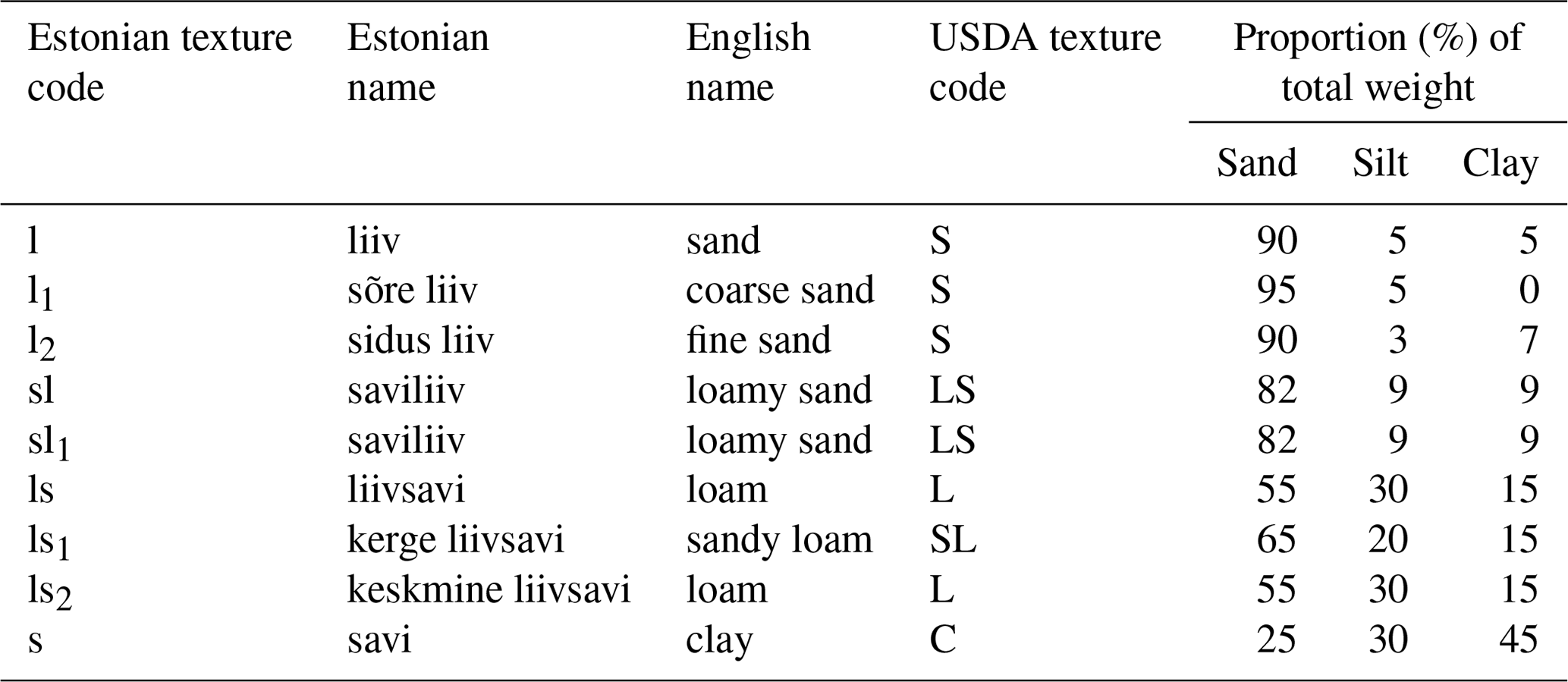
We developed a computer program that converts the encoded texture codes into an intermediate data structure, which extracts again Estonian texture classes and coarse fragment classes, into separate layers including depth information. Subsequently, we derived all defined numerical texture values using a lookup table (Table 1) that represents our best efforts to account for the size difference between the USDA and Soviet systems and lack of silt data in the Soviet system. The foundational numerical values for fine-earth fractions and coarse fragments of the soil are solely derived from the extracted processed Estonian texture classes as demonstrated in Table 1.

In addition we introduced two more classes beyond the well-known USDA textures classes, i.e. “PEAT” and “GRAVELS”. The former states that this soil unit is a peatland, where the peat layer thickness is at least 30 cm. For hydrological modelling reasons we decided to still assign sand, silt, and clay fractions to these units in order to provide soil data coverage with as little interruption as possible. To soil units with the class “PEAT” a high clay content was assigned in order to represent the low vertical conductivity at the bottom of these peat bogs. However, for applications that critically evaluate clay content for soil units, the additional “PEAT” texture class can be used to apply additional rules to mask these soil units accordingly. The latter class “GRAVELS” is intended to demark soil units or discrete layers therein, where only a coarse fragment type but no fine textures have been coded in the original texture codes. In these cases, depending on the type of the coarse fragment the layer can consist of gravels, large rocks, or massive rock.

Table 1 Example of the basic rules for deriving numerical values for texture (sand, silt, and clay contents) from the Estonian texture codes and assigned new English-language and USDA texture classes. These rules were selected by the authors. The full table is provided as a supplemental Excel spreadsheet (“texture_rules_lookup.xlsx”)

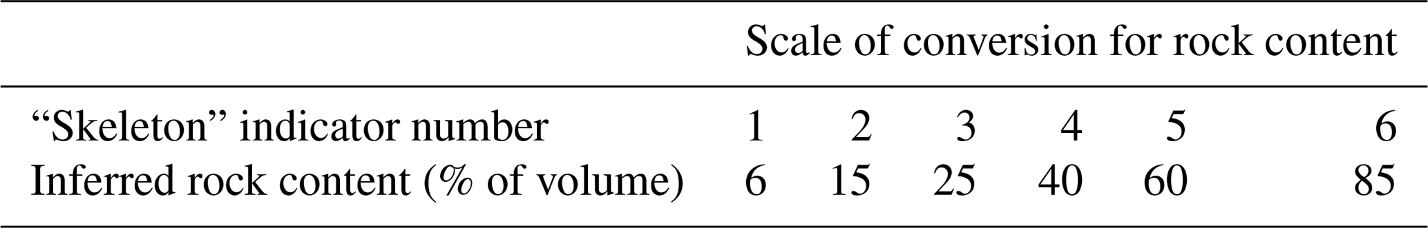
Similar to the Estonian texture classes there exist Estonian stoniness classes that describe a certain type of coarse fragment within the soil profile. An additional number in connection with this rock type identifier indicates the amount or volume of these rocks in 1 kg of soil. We used this indicator number to designate numerical values for the coarse fragments. Table 2 shows how we derived the rock content from the coarse fragments indicator that we obtained from the soil map encoding.

A base assumption is that most soils in Estonia were sampled to a depth of 1 m, as this is the case for a default soil profile. There is only one vertical profile defined per mapped soil unit. If larger or smaller depth information was encoded in the original soil texture code, then this would be used for the overall depth of that soil sample. For each of the layers, we collated depth from the soil surface to the bottom of each layer. The data model is relational and each soil unit is represented as one row, with its polygon geometry, identifier, and all collected parameters as attributes. The maximum number of distinctly defined layers was four, and layer-dependent parameter values (at different depths) are only meaningful where the variable's number suffix is smaller than or equal to the number of defined layers.

Table 2 The relationship between the coarse fragment (rock content and shape) indicator from the soil map encoding and the rock content as a percentage of the total volume. We used the average of each defined range.

We compared the encoded Estonian soil type from the original soil map in order to find the most appropriate soil type from the main Estonian soil types from the soil reference list. The soil types and the Estonian soil names were then related to the FAO WRB soil reference groups (FAO, 2015) after the data have been corrected and standardized for each map unit in the extended soil dataset based on expert input (Hiederer et al., 2011). The full table that relates the Estonian and WRB soil reference groups is provided with the supplemental materials.

This first and fundamental step concluded with a set of variables for each mapped soil unit that now include separate standardized Estonian and USDA texture classes per soil layer, number, and depths of layers of the mapped soil unit and numerical values for fine-earth and coarse fragments fractions per layer, as well as a WRB soil designation group.

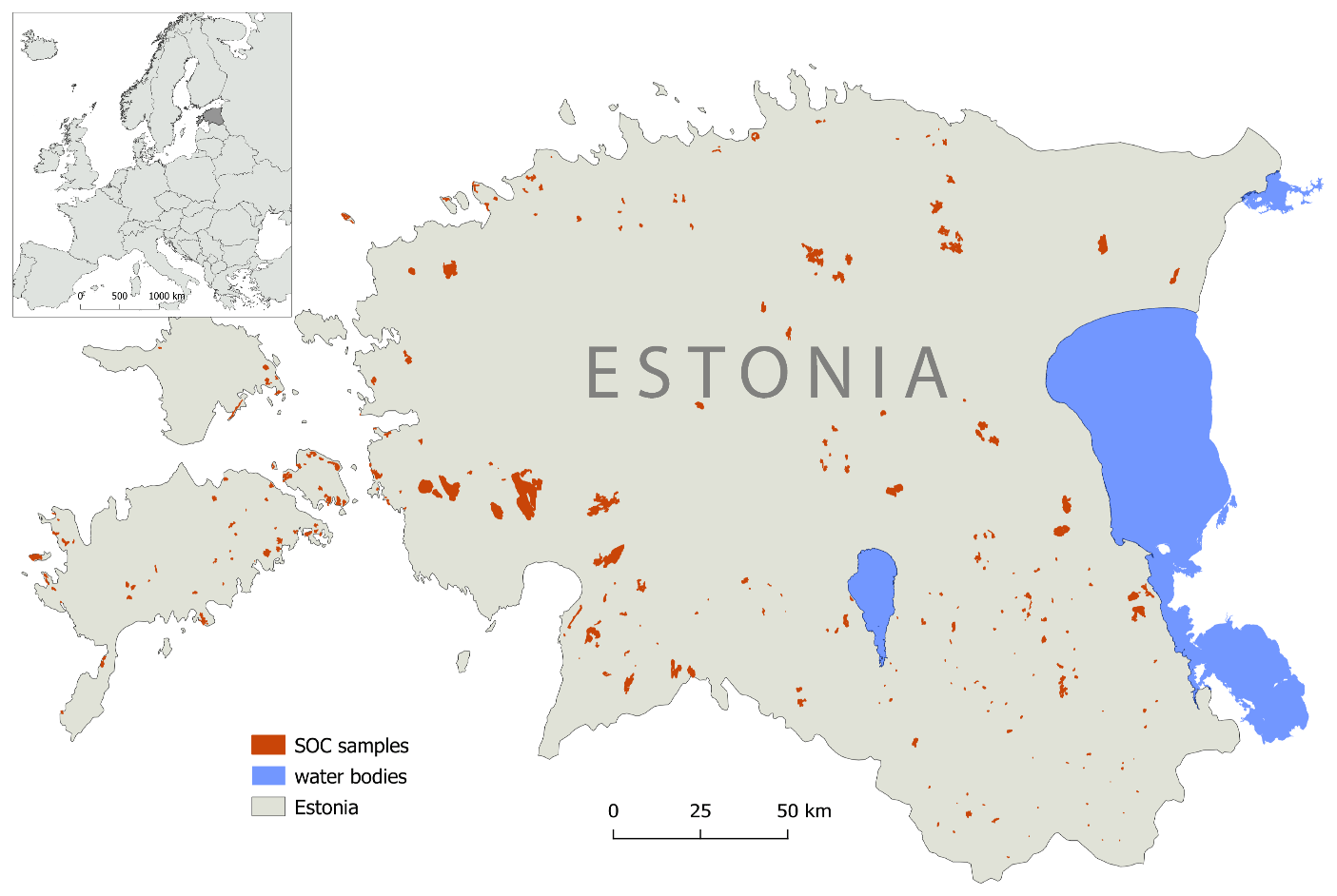
Figure 2 Distinct soil unit polygons including all sampling locations for the machine-learning training sample.

2.3 Adding topographic variables as predictor variables

For the subsequent step of SOC prediction via the random forest machine-learning model, we calculated the mean, median, and standard deviation of several topographic and environmental variables as additional predictor variables. Topographic variables slope, topographic wetness index (TWI), terrain ruggedness index (TRI), and slope length–steepness (LS) factor were all calculated by using SAGA-GIS software based on a digital elevation model (Conrad et al., 2015). The lidar-based digital elevation model with resolution 5 m was obtained from Estonian Land Board.

The TWI is a topo-hydrological factor proposed by Beven and Kirkby (Beven and Kirkby, 1979) and is often used to quantify topographic control on hydrological processes (Michielsen et al., 2016; Uuemaa et al., 2018) which are also relevant in the soil evolution. TWI represents the spatial pattern of saturated areas, which directly affect hydrological processes at the watershed scale (Mokarram et al., 2015).

It is a function of both the slope and the upstream contributing area:

$$\begin{array}{}\text{(1)}& \mathrm{TWI}=\ln (a/\tan b),\end{array}$$

where a is the specific upslope area draining through a certain point per unit contour length (m² m⁻¹), and b is the slope gradient (in degrees).

TRI reflects the soil erosion processes and surface storage capacity which again is relevant from a soil evolution perspective. The TRI expresses the amount of elevation difference between neighbouring cells, where the differences between the focal cell and eight neighbouring cells are calculated:

$$\begin{array}{}\text{(2)}& \mathrm{TRI}=Y{\left[\sum {\left(x_{ij}-x_{\mathrm{00}}\right)}^{\mathrm{2}}\right]}^{\mathrm{1}/\mathrm{2}},\end{array}$$

where x_ij is the elevation of each neighbour cell to cell (0,0). Flat areas have a value of zero, while mountain areas with steep ridges have positive values.

The potential erosion in catchments can be evaluated using LS as used by the universal soil loss equation (USLE). LS is the length–slope factor that accounts for the effects of topography on erosion and is based on slope and specific catchment area (as substitute for slope length). In SAGA-GIS the calculation is based on the following (Moore et al., 1991):

$$\begin{array}{}\text{(3)}& \mathrm{LS}=(n+\mathrm{1})(A_{\mathrm{s}}/\mathrm{22.13}{)}^n(\sin \mathit{\beta }/\mathrm{0.0896}{)}^m,\end{array}$$

where n=0.4 and m=1.3.

In addition, we calculated the area per mapped soil unit in square metres and in percentage of area, which is under drainage. The drainage regime considered both underground tile drainage and ditch-based drainage systems. Analogously, we sorted land use and land cover proportions into arable land, forest, grasslands, wetland, urban areas, water, and “other”, also as area per mapped soil unit in square metres and in percentage of area. The drainage, land use, and land cover information was derived from the Estonian Topographic Database (ETAK) and the official register of drainage systems by the Agricultural Board of Ministry of Rural Affairs of Estonia.

2.4 Predicting soil organic carbon (SOC) and bulk density (BD)

The main information retrievable from the Soil Map of Estonia is only the soil type and the soil texture. However, soil hydraulic properties and SOC data are needed for many different applications in soil hydrology, ecology, and ecosystem services modelling. Pedotransfer functions (PTFs) have proven to be useful to indirectly estimate these parameters from more easily obtainable soil data (Van Looy et al., 2017). Therefore, several soil parameters like soil organic carbon, bulk density, and saturated hydraulic conductivity must be derived via PTFs and other data assimilation methods. To apply PTFs and other data-assimilation methods, third-party datasets can be used as secondary sources. In the previous steps we have prepared a wide set of input variables, including the numerical fractions for the textural properties, standardized classes for soil type and soil textures, and additional topographic variables, which we can apply as predictor variables to model the value distribution for SOC and BD. We develop these two extended soil physical input parameters as organic carbon content in percentage of soil weight and dry bulk density in cubic megagrams per cubic metre (Mg m⁻³) or grams per cubic centimetre (g cm⁻³).

In order to map the spatial distribution of SOC in Estonia a random forest (RF) model was used to predict SOC based on parameters derived from the soil map. RF was preferred to more advanced machine-learning algorithms (e.g. neural networks) because it has been shown to be relatively resilient towards data noise (Breiman, 2001; Caruana and Niculescu-Mizil, 2006). In addition, feature importance can be extracted from the model to determine the most influential predictor variables.

For training, we used measurements of soil organic matter (SOM) or SOC from forest areas (samples sizes: n=100), four datasets of samples from Estonian open and overgrown grasslands and alvars (a type of calcareous grassland on a limestone plain with thin or no soil; n: 94, 137, 146, 69), peatlands (n=175) and arable soil transects (n=8964) resulting in 3373 distinct point locations (Kriiska et al., 2019; Noreika et al., 2019; Suuster et al., 2011). Where necessary, the SOM values were translated into SOC via SOC = SOM∕1.724. Many samples from peatlands and arable fields were often sampled within the same mapped soil unit. For these soil units (polygons) the respective soil measurement data were averaged and joined to the respective soil units to reduce the bias of the prediction. After joining the sample size was reduced to the 397 distinct training samples for machine learning (Fig. 2).

These data were then randomly split into training (60 %) and test (40 %) sets, and the model was evaluated by predicting SOC based on the predictor variables of the test set. Finally, the model was applied to soil map polygons without available SOC measurements to predict SOC content in Estonian soils.

Subsequently, we calculated soil bulk density based on predicted soil organic carbon for each layer in each mapped soil unit polygon, with the following PTF (Adams, 1973; Kauer et al., 2019), which has been successfully applied in Estonia:

$$\begin{array}{}\text{(4)}& \mathrm{BD}=\mathrm{1}/(\mathrm{0.03476}\times \mathrm{SOM}+\mathrm{0.6098}),\end{array}$$

where SOM = SOC ×1.724

The conversion factor of 1.724 is a widely used universal value. However, we acknowledge that the real value varies slightly between soils.

2.5 Assimilation of additional hydrological variables

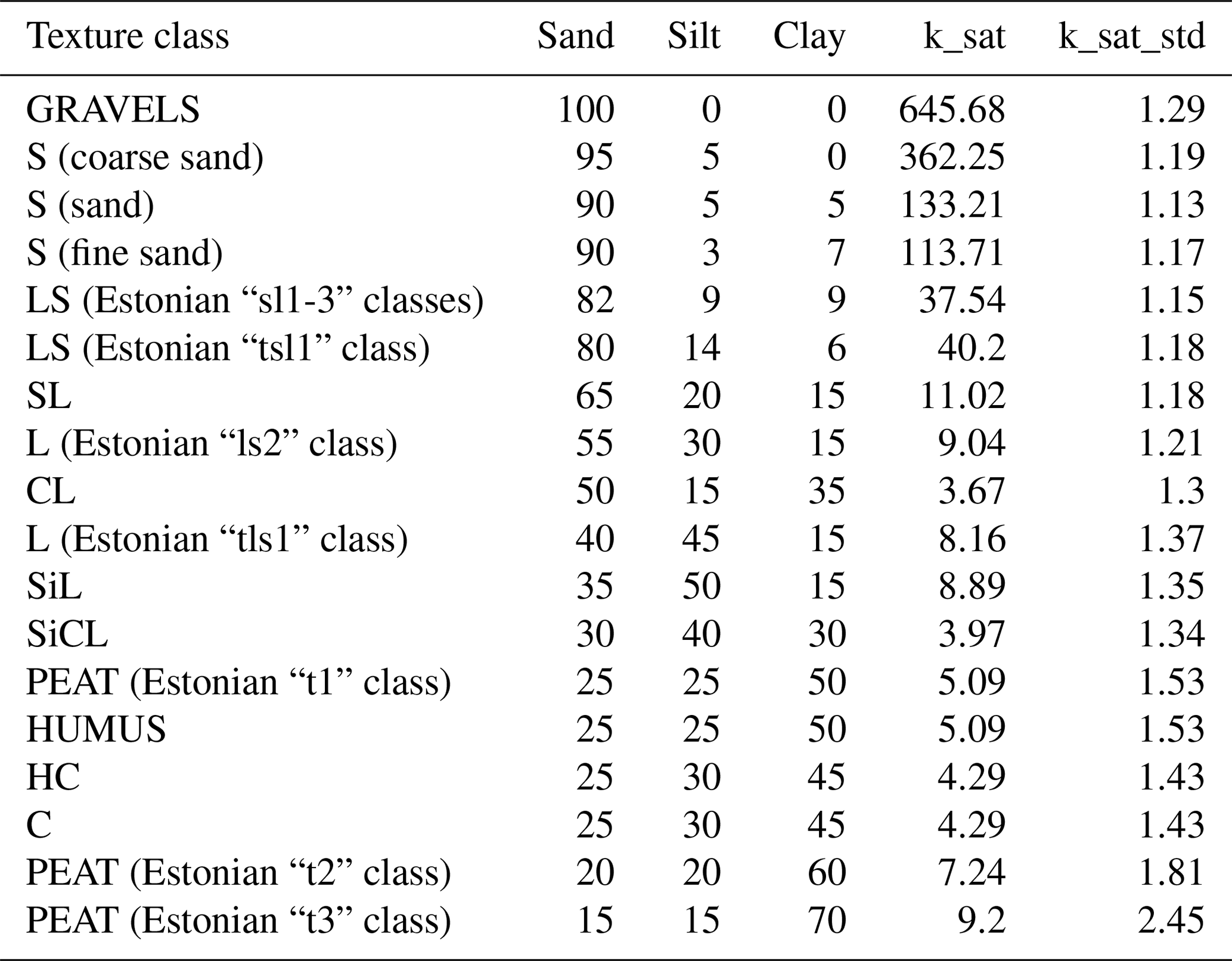
In order for this dataset to be more useful in eco-hydrological modelling we developed and added two additional hydrological variables. Saturated hydraulic conductivity (K_sat) is a quantitative measure of water movement through a saturated soil. In addition to the ability of transmitting water along a hydraulic gradient we also add available water capacity (AWC) as a variable. AWC describes the soil's ability to hold water and quantifies how much of that water is available for plants to grow. We develop two variables: saturated hydraulic conductivity (mm/h) and available water capacity of the soil layer (mm H₂O per millimetre of soil). We calculated K_sat using the improved Rosetta3 software, which relates soil texture to a hydraulic gradient and implements a pedotransfer model with improved estimates of hydraulic parameter distributions (Zhang and Schaap, 2017). It is based on an artificial neural network (ANN) for the estimation of water retention parameters, saturated hydraulic conductivity, and their uncertainties. For each standardized texture class, we used the numerical fine-earth fractions for sand, silt, and clay as inputs for the Rosetta3 software and calculated K_sat for each layer in each mapped soil unit polygon. Table 5 demonstrates the predicted values for several texture classes.

In order to calculate available water capacity, we summarized the field capacity (FC, at −330 cm matric potential) and wilting point (WP, at −15 848 cm matric potential) variables of the seven soil depths of the EU-SoilHydroGrids 250 m resolution raster datasets (Tóth et al., 2017) for each mapped soil unit for the provided depths of 0, 5, 15, 30, 60, 100, and 200 cm. The available water capacity is then calculated for each of the seven depths: AWC = FC − WP (Dipak and Abhijit, 2005). The resulting seven AWC raster layers are then averaged into the respective depth ranges for each of the discrete layers of the Estonian mapped soil units.

3 Results

In this study, we developed the EstSoil-EH database, which includes standardized soil type and soil texture data from the official Soil Map of Estonia, related to the World Reference Base and FAO soil classes and USDA texture descriptions. Figure 3 shows a map of the classified topsoil texture classes derived from the original Estonian texture codes. In addition, it shows the peat soils that cover up to 20 % of Estonia and are an important soil type in such northern countries.

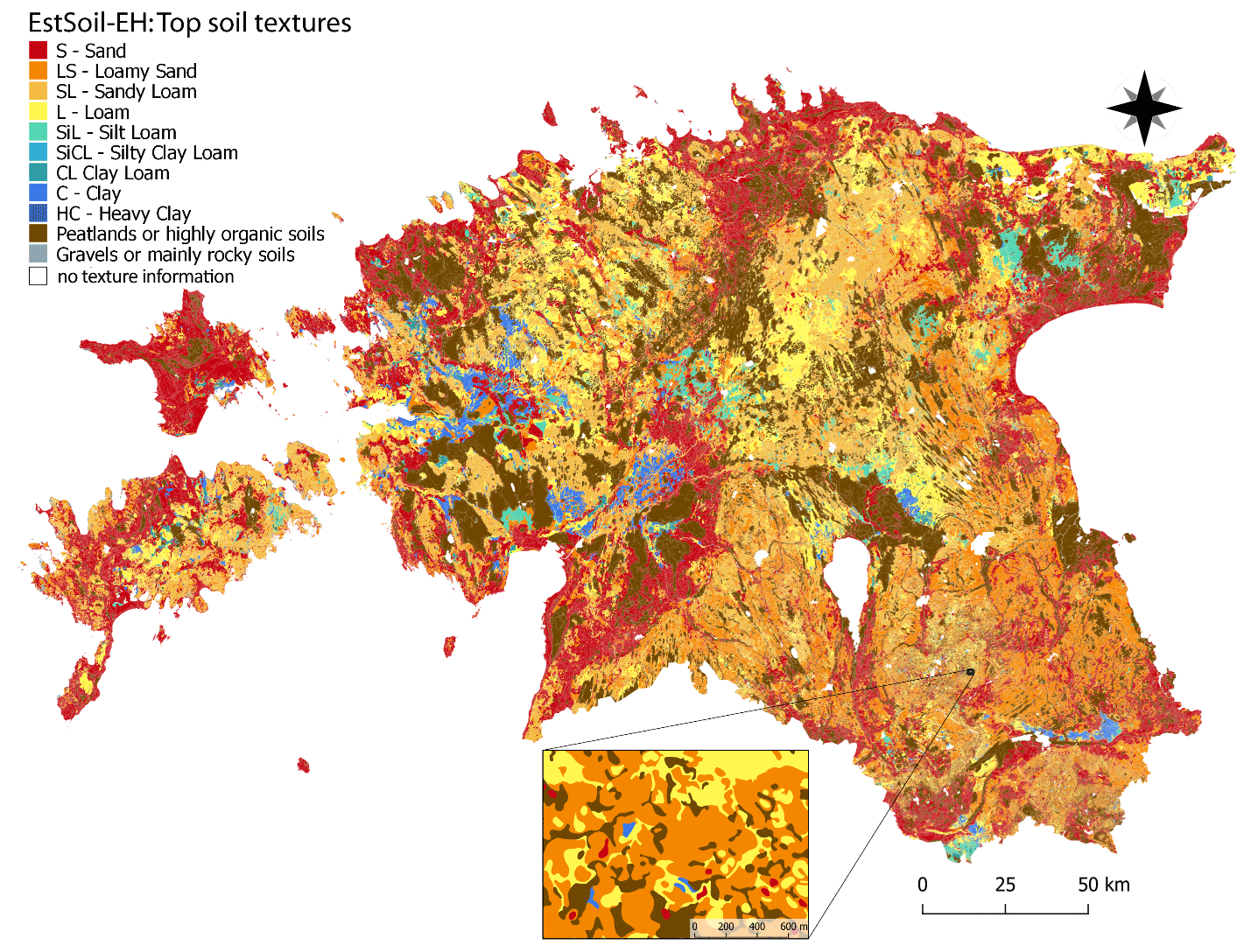
Figure 3 EstSoil-EH dataset: USDA topsoil textures derived from the original Estonian texture codes by the software developed in the present study, including additional classes “PEAT” and “GRAVELS”. Lower image is a zoom-in to a small region to visualize the high level of detail.

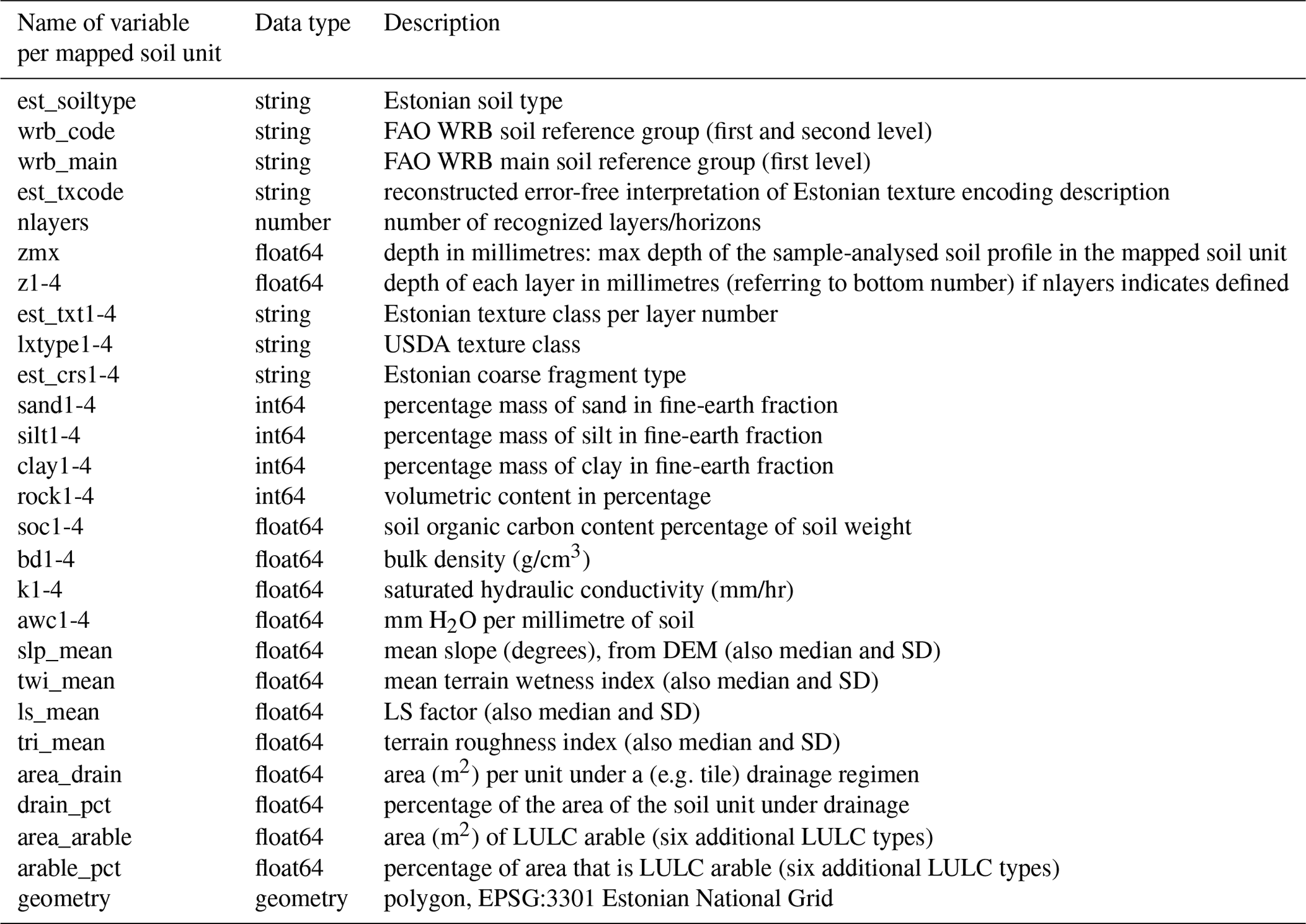
We synthesized additional information usable in an eco-hydrological modelling context for each of the soil units. These values include the number of discretized soil layers – up to a maximum of four separate vertical distinct soil layers where described in the original texture codes – the depth of each layer, and the maximum depth of the sampled profile for each mapped soil unit. Based on the layer information and the texture classes we defined the percent fractions per volume of sand, silt, clay, and coarse fragments per layer. We also added topographical, land use, and land cover information and used these as predictors for SOC. Subsequently, predicted SOC, BD, hydraulic conductivity, and assimilated AWC values were added. Table 3 contains the full list of variables and parameters per mapped soil unit contained in the EstSoil-EH dataset.

Table 3 Description of variables and parameters available in the EstSoil-EH dataset.

3.1 Validation of soil type and texture classes extraction and standardization

For the main soil types, we achieved 97.7 % agreement between the software's result and the manual classification. The manual verification of the validation revealed several re-labelling issues from the error lookup table. A visual assessment by two soil sciences senior research staff members asserted that the level of similarity of the soil types that were selected by the automated process was closely related. However, the mismatches (1943 records, equivalent to 2.3 % of the total records) indicated that the soil experts tended to interpret “errors” based on personal knowledge that may not be reproducible in a strictly automated fashion. For example, some landforms (e.g. eroded material filling low slopes or collapsed cliffs) were originally classified as exceptions to the general classification rule based on the local knowledge of the landscape. When standardizing these expert interpretations with the same more general soil type, we reduced the number of mismatched soil type identifiers to 0. We consider the high accuracy (97.7 %) to be a very good result for a manual approach.

For the validation of textures, we used several steps. First, given the high agreement between the software-generated codes and the human-generated codes, we accepted the software's texture codes for use in our subsequent evaluations. Next, we compared the extracted main texture for each layer with the manually coded value:

• 77 870 of 83 364 records (93.4 %) showed identical parsing of the full texture code.

• 71 635 of the records (85.9 %) showed identical interpretation of the first layer's texture type (10 312 records were differently coded, and 1417 produced “no value” errors, in which either the source or validation dataset contained no value, preventing a comparison with the other dataset's value).

• 65 000 of the records (78.0 %) showed identical interpretation of the second layer's texture (with 2325 differently coded textures, and 16 038 “no value” errors, of which 15 461 occurred in the new automatically processed dataset, and only 577 occurred in the validation dataset).

• 82 507 of the records (99.0 %) showed identical interpretation of the third layer's texture (with most errors caused by a non-existent third layer, 334 differently coded, and 523 with a “no value” error).

For sand, silt, and clay fractions we could obtain laboratory analysis only for 84 forest soil samples. We calculated the root mean squared error (RMSE) and chose the normalized median absolute deviation (nMAD) as an additional measure of dispersion of error for non-Gaussian distributed data:

• RMSE for sand: 13.1 %;

• nMAD for sand: 9.68 %;

• RMSE for silt: 10.7 %;

• nMAD for silt: 7.0 %;

• RMSE for clay: 6.5 %;

• nMAD for clay: 3.9 %.

Our manual assessment of the mismatches indicated the same problem that occurred with the soil types. The expert assessments aimed to keep as much information as possible available in their decoded classification, and this did not always agree with the automated processing rules. In addition, to derive the grammar rules, we added a few simplifying elements, such as omitting some rarely used additional information in the soil texture descriptions. For example, the Estonian rules allow specification of several soil parts, but as a horizontal distribution within the same mapped soil unit rather than as vertical layers. This is understandably complex, making it difficult to classify this variable soil as a single soil unit. Consequently, it is inevitable that some of these descriptions will not agree with the software's classification.

3.2 SOC prediction and validation of a random forest model

We also calculated several extended soil properties, i.e. SOC content and BD. The RF regression model was implemented with the RandomForestRegressor function from the Scikit-learn Python library (Pedregosa et al., 2011). The model was evaluated by predicting SOC based on the predictor variables of the test set for the 60:40 split. Figure 4 illustrates the cross-validation scatterplots of observed vs. predicted SOC values for the test–validation sample splits. The following characteristics are reported for the chosen RF model:

• coefficient of determination (R²) score: 0.69;

• score of the training dataset with out-of-bag estimate (oob score): 0.58;

• Pearson's r correlation coefficient, training: 0.90, validation: 0.83.

The top six RF features of importance are as follows:

• clay content (CLAY1): 0.65;

• terrain roughness index, standard deviation (tri_stdev): 0.04;

• sand content (SAND1): 0.03;

• LS factor, median (ls_median): 0.028;

• area under drainage in percent (drain_prct): 0.027;

• coarse fragments rock content (ROCK1): 0.024.

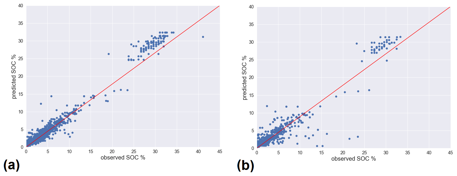
Figure 4 Random forest model cross-validation scatterplot of observed vs. predicted SOC values for the test–validation sample splits: (a) training subsample and (b) validation subsample.

Figure 5 shows the predicted values of SOC for the top layer. On visual inspection the spatial distribution for the SOC content matches comparatively well with known agricultural areas, where low carbon content prevails, as well as with the peat land areas, which have a very high carbon content.

For further description and guidance on errors in the predictions for SOC and BD we calculated the RMSE and nMAD as an additional measure of dispersion of error for non-Gaussian distributed data. BD-observed data were only available for arable lands and forest soil samples and should be treated accordingly.

• RMSE for SOC predictions: 2.95 %;

• nMAD for SOC: 1.44 %;

• RMSE for the subsequent BD predictions with PTF: 0.33 g/cm³;

• nMAD for BD: 0.15 g/cm³.

However, due to the small number and distribution of input samples over four distinct land cover types, namely arable lands, wetlands, forests, and open or grass lands, we evaluated the error distribution for each land form in Table 4. The prediction error characteristics differ, with the smallest errors for arable lands, then wetlands and the largest for open grasslands and forest.

Table 4 Statistical description of SOC prediction error per land form.

Figure 5 Predicted soil organic carbon (SOC) of the top soil layer.

3.3 Hydrological variable results

Based on the variables derived in previous steps, we could calculate saturated hydraulic conductivity (K_sat) based on the sand, silt, and clay content. Rosetta3 reports the standard deviation for its internal prediction process, which draws many samples for the same input of sand, silt, and clay content and then provides the mean as the predicted value for K. The summary of the predicted K_sat values and the standard deviation are summarized in Table 5. For peat areas and wetlands the predicted values also correspond with ranges reported in the literature for the sand–silt–clay ratios provided (Gafni et al., 2011).

Available water capacity was calculated solely by aggregating EU-SoilHydroGrids data for field capacity and wilting point (Tóth et al., 2017). We compiled all parameters into a dataset that can now be easily used with SWAT or other eco-hydrological and land-use-change models. As we are not changing the general geometry or underlying spatial data model of the original soil map, all parameters are only added to the existing mapped soil units, and thus all original soil polygons remain discernible.

Table 5 Predicted K sat values in mm/h and reported standard deviation from Rosetta3.

4 Code and data availability

The described “EstSoil-EH” dataset including all supplemental tables and figures is deposited on Zenodo, https://doi.org/10.5281/zenodo.3473289 (Kmoch et al., 2019a). Supplemental software and codes that were used, e.g. the texture-code parsing scripts, the machine learning model, and the parameter calculation Jupyter notebooks, are maintained on GitHub (https://github.com/LandscapeGeoinformatics/EstSoil-EH_sw_supplement/releases, last access: 10 January 2020) and were also deposited on Zenodo, https://doi.org/10.5281/zenodo.3473209 (Kmoch et al., 2019b). The original National Soil Map of Estonia (https://geoportaal.maaamet.ee/est/Andmed-ja-kaardid/Mullastiku-kaart-p33.html, last access: 10 January 2020) was archived for reference on the DataCite- and OpenAire-enabled repository of the University of Tartu, DataDOI, https://doi.org/10.15155/re-72 (Estonian Landboard, 2017).

5 Discussion and future work

For EstSoil-EH, we derived numerical values for the following data in all of the mapped soil units in soil map: soil type (i.e. soil reference group), texture class, soil profiles (e.g. layers, depths), texture (clay, silt, sand components, and coarse fragments), rock content, and physical variables related to the water and carbon cycle (organic carbon content, bulk density, hydraulic conductivity, available water capacity). Before our analysis, a large amount of the information from the high-resolution Soil Map of Estonian was not readily usable beyond the field or farm scale because of the need to manually interpret the specialized soil types and the complexity of the rules that describe the texture or other characteristics of the soil units. We provide an extended ready-to-use dataset containing additional parameters. We also describe the development of a reproducible method for deriving these numerical values from a national survey-based soil map to support modelling and prediction of eco-hydrological processes and ecosystem services. Thus, our presented dataset holds the potential to further improve our understanding of eco-hydrological processes in the landscape through the use of advanced statistical (e.g. machine learning) and process-based models. The information derived is much more spatially related to the landforms and land use observed there than any other dataset covering soil information for Estonia. Furthermore, the textures and SOC and BD values are directly derived from reliable observed data samples from Estonia. This is unique in the case of Estonian soil datasets and does not hold true for many other reported soil datasets that cover the area of Estonia. However, the complexity of the Estonian texture rules and the reliance on human judgement creates high uncertainty in some cases, even for human interpretation. For example, it is not possible to retrospectively redefine minor differences in boundaries between different classes between texture systems, but we consider natural variation of texture within the soil mapping unit at a scale of 1:10 000 more significant than that of different texture systems.

Our reproducible workflow and the open-access availability and transparency of measurement data can provide a reliable building block for advancing the study of soil and hydrological processes in Estonia into temporal aspects. In particular, properties such as SOC and BD will vary extensively depending on the land use and land cover. In combination with developments that also capture the dynamics of land use change and adaptations under climate change, the evolution of the soils in Estonia could more readily be investigated.

One challenge in SOC modelling was that the number of field-based samples that were used for training the random forest model was relatively small for the whole country. Even though the samples covered four main land cover types (agricultural, forests, wetlands, grasslands), there was still significant spatial heterogeneity that might not have been captured. Moreover, in addition to field-based validation data, we used lower-resolution modelled datasets, e.g. SoilGrids and EU-SoilHydroGrids, for a comparative validation. These datasets are not necessarily more accurate than the results of our classification. Although we accounted for this problem by providing additional comparisons, the scale mismatch between continuous raster datasets and polygon-based data inevitably introduced errors and trade-offs into the comparison. One solution to these problems would be to perform supplemental field sampling to ground-truth the source data and confirm the accuracy of our model's classification based on the field data.

From the point of the end-user, the first layer is not a default 30 cm deep top soil layer. A direct interpretation of the derived discrete layer information as soil horizons should not be generalized but checked on case-per-case basis. All physical, chemical, and hydraulic properties are based on the analysis of the original texture code per mapped soil unit and the resulting discrete layers per unit. This is an important usage constraint, for example in the sense of biological activity, as the 30 cm soil layer is the most active, but for each soil unit it needs to be checked which layers extend into which actual depths. Also, the SOC content and BD are not modelled in a vertical continuum but per discrete value per unit and layer. However, fertile soils like Luvisols contain a lot of SOC, also in deeper layers. But such additional expert knowledge is encoded neither in the original Soil Map of Estonia nor in the processing algorithms that derived the extended parameters for this newly generated dataset. However, such additional knowledge, as well as more appropriate models for peatland areas, could be included as additional rules in a subsequent improvement of this dataset.

Kõlli et al. (2009) published estimates of the SOC stocks for forests, arable lands, and grasslands and for all of Estonia. Nevertheless, they constrained their finding by noting that their estimates were calculated based on the mean SOC stock for each soil type and the corresponding area in which the soil type was distributed. Putku (2016) used the large-scale Soil Map of Estonia at the polygon level for SOC stock modelling for mineral soils in arable land of Tartu county. Carbon content calculations in Estonia have historically been predominantly made for soils in agricultural areas. Existing literature and our results in summary are in line with SOC distribution per soil type in mineral soils in arable lands (Suuster et al., 2011).

The original purpose of this dataset was to derive values for hydrological modelling purposes and at the same time to stay as close to the original data as possible. From that perspective peat soil units are currently modelled with assumptions to have a similar behaviour to clay hydrologically. Therefore, the spatial distribution of clay percentage in particular, but also the concurrent physical fractions of sand and silt do not make scientific sense for these areas where peat is prevalent. In order to make the dataset as useful as possible and to identify peatland areas, we introduced the additional class “PEAT” into the USDA classification. While sand, silt, clay, and rock content are directly derived values from the original texture codes, SOC and K_sat are modelled via statistical machine-learning algorithms, which include additional uncertainty. This should be considered when evaluating BD, which is calculated using SOC as an input variable. In addition, it would be possible to use BD as an additional predictor for Rosetta3. However, we decided that this would introduce too much uncertainty as BD in EstSoil-EH is based on a PTF function of SOC, which in turn was also predicted via statistical modelling.

The only variable which we did not model based on the dependence of already modelled parameters was AWC. Here we summarized the EU-SoilHydroGrids 250 m (Tóth et al., 2017) raster datasets for FC and WP as inputs for an external data integration. This is not ideal and can be considered a trade-off between introducing too much uncertainty and an external unrelated data source.

In the future, we foresee step-wise improvement of our software by developing better PTFs to estimate parameters and to better integrate the presence of peat soils and other specific landscapes and environments in Estonia. Furthermore, statistical machine-learning, neural-network, and deep-learning methods could be tested in order to improve soil classifications and express more complex relationships between soil types and textures. Currently, one specificity of the newly created EstSoil-EH dataset is its discrete nature, as we are only adding derived numerical variables to the existing mapped soil units (polygons). We do not predict a continuous surface in this study; thus, comparisons with continuous surface parameters predictions such as in SoilGrids (Hengl et al., 2017) or EU-SoilHydroGrids (Tóth et al., 2017) are not directly possible. However, the workflow could also potentially be extended for creating a continuous surface. With appropriate modification (e.g. to use the soil characteristic codes more consistently for a different country), our methodology could also be applied in other countries such as Lithuania or Latvia that share similar historical land- and soil-surveying practices.