Real-time WRF large-eddy simulations to support uncrewed aircraft system (UAS) flight planning and operations during 2018 LAPSE-RATE

The simulation dataset described herein provides a high-resolution depiction of the four-dimensional variability of weather conditions across the northern half of the San Luis Valley, Colorado, during the 14–20 July 2018 Lower Atmospheric Profiling Studies at Elevation-A Remotely-Piloted Aircraft Team Experiment (LAPSE-RATE) field program. The simulations explicitly resolved phenomena (e.g., wind shift boundaries, vertical shear, strong thermals, turbulence in the boundary layer, fog, low ceilings and thunderstorms) that are potentially hazardous to small uncrewed aircraft system (UAS) operations. Details of the model configuration used to perform the simulations and the data-processing steps used to produce the final grids of state variables and other sensible weather products (e.g., ceiling and visibility, turbulence) are given. A nested (WRF) model configuration was used in which the innermost domain featured large-eddy-permitting 111 m grid spacing. The simulations, which were executed twice per day, were completed in under 6 h on the National Center for Atmospheric Research (NCAR) Cheyenne supercomputer using 59 cores (2124 processors). A few examples are provided to illustrate model skill at predicting fine-scale boundary layer structures and turbulence associated with drainage winds, up-valley flows and convective storm outflows. A subset of the data is available at the Zenodo data archive (https://zenodo.org/record/3706365#.X8VwZrd7mpo, Pinto et al., 2020b) while the full dataset is archived on the NCAR Digital Asset Services Hub (DASH) and may be obtained at https://doi.org/10.5065/83r2-0579 (Pinto et al., 2020a).

1 Background

The LAPSE-RATE field program took place 14–20 July 2018 in the San Luis Valley (SLV) of Colorado. The goal of this project was to utilize a fleet of small uncrewed aircraft systems (UASs) to sample sub-mesoscale variability occurring in the lower atmosphere of an alpine desert valley that resulted from surface–air interactions within complex terrain characterized by heterogeneous surface conditions (de Boer et al., 2020a). Several meso-gamma-scale (i.e., 2–20 km in extent) circulations were expected including drainage winds, valley flows and thunderstorm outflows; however, the extent, strength and depth of these flows was not well-known due to a lack of observations in the area. The impact of surface heterogeneities (specifically, irrigated cropland versus fallow fields and desert shrubland) on boundary layer evolution and their influence on triggering moist deep convection was also targeted with UAS missions.

The process of driving a large-eddy simulation (LES) model with time-varying mesoscale forcing at the lateral boundaries is known as mesoscale-to-microscale (M2M) coupling (Haupt et al., 2019). The need for LES-permitting environmental prediction spans many economic sectors, including applications in wind energy (Olson et al., 2019), hydrometeorology and flash-flood prediction (Silvestro et al., 2019), and precision agriculture (Tesfuhuney et al., 2013). In addition, accurate wildland fire prediction requires simulating the impact of fine-scale terrain features on air flows as well as fire–weather feedbacks that occur at scales of less than 100 m (Jiménez et al., 2018). In wind energy, wind farm operators need a high-resolution (in space and time) depiction of wind variation across their turbine arrays in order to estimate energy output (Liu et al., 2011). Early on, Bryan et al. (2003) demonstrated the importance of resolving fine-scale flow features in order to accurately simulate the evolution of tornado- and flash-flood-producing supercell convective storms.

The use of small UASs in commercial applications has grown immensely over the past few years, and routine flights beyond visual line sight will soon be performed. This paradigm shift will require improved weather guidance products to support safety and efficiency. The performance and recoverability of small UASs are influenced by weather conditions (e.g., gusty winds, vertical wind shear, wind shift boundaries, thermals) that are considered benign by general aviation. Small UASs are susceptible to these conditions because of their lighter weight, weaker thrust and limited energy supply (Ranquist et al., 2017). In addition, keeping small UASs within the visual line of sight (which is an FAA Part 107 regulation for many current small UAS operators) can quickly become problematic under a range of conditions including development of fog, lowering cloud bases, and haze/pollution and sun angle considerations. As commercial uses of small UASs continue to expand, fine-scale weather information at scales much smaller than those currently resolved by operational numerical weather prediction (NWP) models will be needed to ensure safety and improve cost-effectiveness of operations (e.g., Campbell et al., 2017; Glasheen et al., 2020; Steiner, 2019; Garrett-Glaser 2020). Campbell et al. (2017) point out that analyses and forecasts of winds and turbulence in the lower atmosphere are currently not adequate for supporting efficient UAS traffic management (UTM), which requires accurate wind information at scales relevant to UAS routing structures. At the same time, Roseman and Argrow (2020) note the importance of accurate, high-resolution analyses and predictions of weather hazards and associated uncertainties to support UAS flight planning.

The LAPSE-RATE field experiment offered an opportunity to work with UAS operators to better understand their needs and potential risks for when operating in a high-alpine-desert environment characterized by a range of small-scale flow patterns. At the same time, atmospheric data collected during the experiment can be used to assess WRF LES predictions and to assess the value of UAS observations in data assimilation experiments (e.g., Jensen et al., 2021). Ultimately, studies are needed to determine the potential value of these very high-resolution simulations in supporting UAS operations versus using output from coarser-resolution mesoscale models that will continue to be operational over the next decade or longer.

The grid-spacing used in operational NWP models has been rapidly decreasing over the past 2 decades but has leveled off in recent years. At grid spacings of less than 1 km, the partial differential equations describing the spatiotemporal evolution of weather begin to resolve circulations in the boundary layer that are treated by planetary boundary layer (PBL) schemes. At the same time, atmospheric turbulence closure schemes used in LES models are not designed to operate at grid spacings greater than ∼ 100 m. Because of these issues, Wyngaard (2004) named this problematic range of model grid spacings (100 m–1 km) the “terra incognita”. Thus, simulating the impact of mesoscale flows on local turbulence properties of the atmosphere requires a substantial increase in the resolution between the mesoscale and microscale grids (e.g., Muñoz-Esparza et al., 2017).

Over the past 5 years, work has progressed on M2M coupling (Haupt et al., 2019). It has been shown that the performance of mesoscale models running at sub-kilometer grid spacing may actually suffer a degradation in skill. Rai et al. (2016, 2019) have shown that the skill of a mesoscale model forecast can actually decrease when using grid spacings of between 0.5 and 1.25 km compared to grid spacings greater than 1.25 km. These findings are important when considering that current operational forecasting centers are beginning to implement grid mesh nests with grid spacing of 1 km or finer. As mentioned above, grid spacings of between 150 m and 1 km are too coarse for sub-grid-scale parameterizations used in LESs to work properly and have been shown to systematically over-estimate turbulence energy content (Doubrawa and Muñoz-Esparza, 2020). Thus, general guidelines for M2M have been developed that recommend avoiding the range of grid resolutions that span the terra incognita.

Another key consideration in M2M coupling is the distance from the LES domain edge required to fully spin up turbulent motions within the LES grid. Muñoz-Esparza et al. (2014) demonstrated that the absence of fully spun-up turbulence in LES can lead to an imbalance between the subgrid scale and resolved scales of motion that not only degrades the turbulence intensity estimates but can also result in a spurious wind speed profile. Markowski and Bryan (2016) have reported that LESs without properly developed turbulence produce unrealistic near-surface vertical wind profiles with excessive vertical wind shear. Muñoz-Esparza and Kosović (2018) have shown that the distance required for turbulent motions to fully develop is related to the ratio of the convective velocity scale and the horizontal mean wind during convective daytime conditions.

These considerations must be taken into account when designing a M2M forecast system. The model configuration used to generate real-time microscale forecast guidance to support both the intensive operation period (IOP) planning and small UAS operations during LAPSE-RATE is described in Sect. 2. Examples of the guidance products that were generated during the experiment and preliminary comparisons with observational datasets are given in Sect. 3. A detailed description of file-naming conventions and data formats is provided in Sect. 4, and data availability is detailed in Sect. 5 with a summary of the work being given in Sect. 6.

2 Model configuration

Version 3.9.1.1 of the Weather Research and Forecasting (WRF) model (Skamarock and Klemp, 2008; Skamarock et al., 2008) was configured and automated to generate twice-per-day fine-scale simulations to support UAS operations. The system was adapted from that developed by Jiménez et al. (2018) to support wildland fire management. Control scripts were developed and adapted to ingest model forcing datasets, convert them to WRF input data formats, execute a nested WRF model configuration and post-process model data to provide UAS weather hazard guidance in real time. Guidance on local winds, thermal patterns and turbulence patterns required implementation of a WRF LES grid (innermost domain in Fig. 1) capable of resolving terrain-driven flows and boundary layer structures on scales relevant for UAS flight planning. The simulations were performed twice per day on the Cheyenne supercomputer (CISL, 2019). The real-time predictions and post-processing were run in under 6 h using 59 cores (2124 processors)¹. Details of the model configuration are given in Table 1 and described further below.

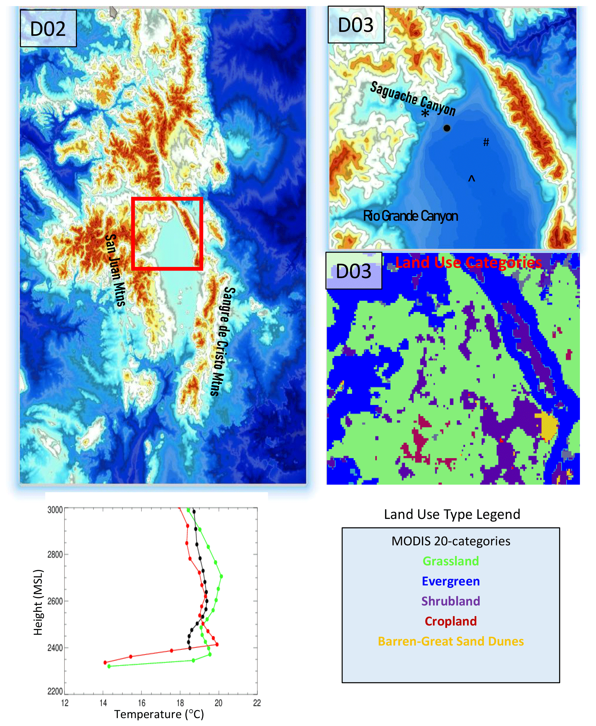
Figure 1 Model terrain for D02 (1 km grid spacing) and D03 (111 m grid spacing) and land use specification for D03 obtained from the MODIS 20-category dataset. Note that D02 was nested within a mesh with 9 km grid spacing when GFS forcing data were used. The symbols “*”, “#” and “∧” mark the location of the AWOS station at Saguache Municipal Airport (SAG), Moffat observing site (MOF) and Leach Airport locations, respectively, for which high-rate model output data are available. The filled circle marks the location of the NSSL soundings. WRF LES profiles of temperature are given for three grid points (closest to SAG (black), NSSL (red), MOF (green)) for the drainage flow case valid at 06:00 MDT on 19 July 2018. The heights of the half levels at each location are indicated by the filled circles.

Table 1 Model configuration.

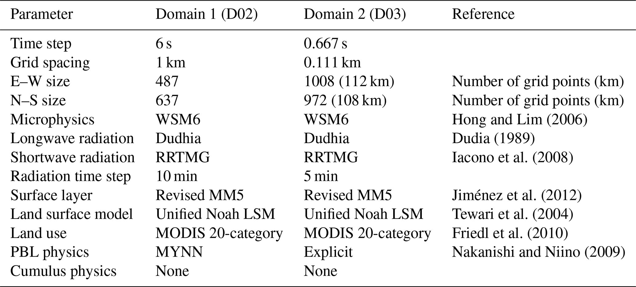
A schematic representation of the run-time configuration is shown in Fig. 2. The simulations used to support next-day planning were driven at the lateral boundaries of D01 (not archived) using forecast data from the 12:00 UTC run from NCEP's Global Forecast System (GFS) model (Version 14). A detailed description of the GFS is provided online (https://www.emc.ncep.noaa.gov/emc/pages/numerical_forecast_systems/gfs/implementations.php, last access: 12 December 2020). The GFS runs at 18 km resolution and uses advanced techniques for assimilation of data collected from platforms ranging from surface met stations to satellites. For day-of planning, D02 was initialized and forced using the 04:00 UTC run of the High Resolution Rapid Refresh (HRRR) model (version 2), also run at NCEP. In addition to hourly cycling to assimilate conventional observations, the HRRR performs 15 min cycling to assimilate radar reflectivity data using latent heat nudging within the grid point statistical interpolation module (Benjamin et al., 2016), producing a new 18 h HRRR forecast each hour. The D02 domain is run for 6 or 16 h depending on the forecast input (HRRR versus GFS, respectively) to allow model dynamics and thermodynamics to come into balance prior to initiating the innermost domain, D03 (referred to as WRF LES hereafter). Sensitivity studies revealed that a 6 h spin-up period provided an adequate amount of time for noise and spurious gravity waves in D02 to dissipate, thus producing well-balanced flows needed to drive the lateral boundaries of D03.

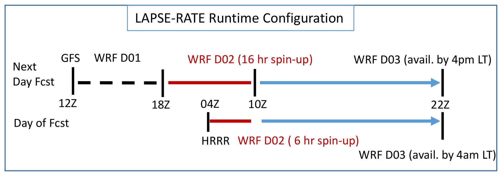
Figure 2 Input, timing and availability for WRF LES simulations which were executed twice per day. Next-day planning guidance was generated using forcing from the 12:00 UTC GFS run while day-of guidance was driven using data from the 04:00 UTC HRRR run. Note that the GFS runs required three concentric nests to downscale from 0.25^∘ to 111 m grid spacing using WRF LES. The dashed black line represents the spin-up period for D01 before D02 is initiated starting at 18:00 UTC. The red solid lines indicate the spin-up period for D02 (1 km grid spacing) in both simulations while the solid blue lines indicate the 12 h period over which WRF LES (D03) was valid. Data from the next-day GFS-forced run were available at 16:00 MDT while data from the day-of HRRR-forced run were available at 04:00 MDT to support UAS flight planning.

In both simulations, the WRF LES domain is initialized at 10:00 UTC with simulations being integrated 12 h out to cover the period of interest for UAS flight planning and deployment. The requirement for simulations to be available for planning purposes dictated the domain configuration, domain size, grid spacing and which operational forecast models were used to drive the prediction system. The runs were generally available at 16:00 (GFS-forced runs) and 04:00 (HRRR-forced runs) MDT (UTC = MDT+7) each day. The run available at 16:00 MDT was used by LAPSE-RATE participants to decide which IOP flight configurations to deploy the next day. The day-of guidance, available at 04:00 MDT, was used to assess whether the weather situation had notably changed from that expected based on the previous day's forecast, with specific emphasis on providing warnings of the potential for conditions that might be hazardous to small UAS operations.

In order to perform simulations with M2M coupling in real time, a refinement ratio of 9 : 1 between the parent domain (D02, 1 km grid spacing) and the WRF LES grid (D03, 111 m grid spacing) was used. This nesting ratio, which is identical to that used by Muñoz-Esparza et al. (2018) and Jiménez et al. (2018), resulted in well-behaved simulations that all completed without error. As discussed above, this large refinement ratio was used to minimize the impact of the terra incognita range of grid resolutions for which boundary-layer parameterizations were not designed (Wyngaard, 2004; Zhou et al., 2014). Using this 9 : 1 refinement ratio allows for use of the MYNN turbulence parameterization (Nakanishi and Niino, 2009) on the 1 km grid mesh (D02) while no PBL scheme is used on the innermost grid, and the model generates its own turbulent motions with the large turbulent eddies being fully resolved. The turbulent kinetic energy (TKE) of the sub-grid-scale motions within the LES grid were diagnosed following the treatment described by Lilly (1966a, b) and formalized in terms of grid-spacing-dependent eddy diffusivities by Deardorff (1980) in their Eq. (6).

While Rai et al. (2019) indicate that the MYNN scheme was prone to developing spurious structures in the PBL at horizontal resolutions comparable to the boundary layer depth, Muñoz-Esparza et al. (2017) found that, in general, the MYNN scheme performed best in simulating the evolution of the boundary layer throughout the diurnal cycle when using model grid spacings of 1 km or greater. In addition, Rai et al. (2019) found that performance of the WRF LES is less sensitive to the PBL scheme used in the parent domain than it is to the sub-grid-scale turbulence parameterization used in the LES domain. A similar conclusion was found by Liu et al. (2020) in simulating flows over complex terrain. Thus, it was decided to use the MYNN scheme, since the simulation period spanned the transition from stable nocturnal morning boundary layer to daytime convective boundary layer.

Finally, it should be noted that the cell perturbation technique outlined by Muñoz-Esparza et al. (2014) was not utilized in this implementation of WRF LES. As it turned out, boundary layer winds were rather weak (i.e., less than 5 m s⁻¹), and surface-based heat fluxes were strong; thus, PBL growth and the evolution of turbulence structures was dominated by local processes and vertical turbulent transport (Muñoz-Esparza and Kosović, 2018). Under these conditions, adding perturbations at the lateral boundaries to aid development of turbulence along the inflow boundaries is not necessary. In addition, the large extent of our domain ensured flow equilibration within the region of interest, which was far removed from the WRF LES lateral boundaries.

Surface fluxes were computed using the revised MM5 surface layer parameterization which includes updates to the Monin–Obukhov-based surface layer parameterization, improving the computation of surface layer fluxes by smoothly extending the stability function over a wide range of stability conditions following Jiménez et al. (2012). This treatment greatly improves the simulation of surface fluxes under more extreme stability conditions experienced during LAPSE-RATE. Land surface type, which determines the surface roughness length and albedo (among other properties) was prescribed using 1 km resolution MODIS 20-category data. Terrain was also prescribed using 1 km data from the U.S. Geological Survey (USGS). General properties of the model configuration and a listing of the physical parameterizations used to produce the simulations are provided in Table 1.

A vertically stretched terrain-following sigma coordinate is used with vertical resolution of less than 150 m in the lowest 1.25 km of the model (Fig. 1). The top of the model was moved from a standard height of 50 to 200 hPa (i.e., omitting model levels in stratosphere) in order to accommodate increased vertical resolution near the surface and timely completion of the simulations. The influence of this reduced model top has been shown to have minimal impact on the evolution of the lower atmosphere (Jiménez et al., 2018). Vertically propagating gravity waves are attenuated using vertical velocity Rayleigh damping within a 5000 m deep layer below the model top with a damping coefficient of 0.2 s⁻¹ (Klemp et al., 2008).

The raw model data were post-processed using a modified version 3.2 of the NCEP Unified Post Processor (UPP; see the UPP User's Guide V3.0 for details, https://dtcenter.org/sites/default/files/community-code/upp-users-guide-v3.pdf, last access: 1 December 2020) and sent to a data server for immediate rendering as images that could be viewed within a web-based display. Modifications to the UPP for this study include adding output fields of relative humidity, TKE and vertical velocity and handling sub-hourly data. Images from the LES grid were used during the daily weather briefings to support next-day flight planning. The UPP was configured to immediately post-process the data from both D02 and D03 (i.e., the LES domain). The UPP was used to de-stagger the u and v components of the wind field so that the wind and mass fields were all on a common grid. Data were also vertically interpolated from the computational sigma coordinate system to flight levels (i.e., meters above ground level). In order to save space, only data from 20 flight levels spanning the lowest 5 km a.g.l. of the simulations are available in the archive. These three-dimensional data grids were stored every 10 min. Fine-temporal-resolution profiles and near-surface variables were stored for select model grid points that corresponded with locations where fixed assets were deployed during LAPSE-RATE (Fig. 1). A detailed description of the file-naming convention and the content of each file stored in the archive is given in Sect. 4.

3 Data products and preliminary assessment

An overview of model performance over the course of the LAPSE-RATE field experiment is shown in Fig. 3 using 10 m wind predictions from all six HRRR-forced (using the 6–18 h HRRR forecast lead times to drive lateral boundaries of D02) simulations. It is noted that the GFS-forced simulations were generally less accurate than the HRRR-forced simulations likely due, in part, to the more coarse resolution and longer lead times (22–34 h forecast lead times) of the GFS used to drive the next-day WRF LES runs. Thus, the analyses hereafter focus on results from the HRRR-forced simulations which give the LES the best chance of matching with the observations. Modeled 10 m winds obtained from both domains are compared with automated weather observing station (AWOS) observations obtained at Saguache Municipal Airport near the mouth of Saguache Canyon (see Fig. 1 for location of the AWOS called SAG). The light blue boxes indicate transition and overnight periods (18:00 to 06:00 MDT). The winds observed at SAG demonstrate a clear diurnal signal each day, with drainage winds from the northwest (i.e., u > 0 and v < 0 m s⁻¹) developing around midnight (00:00 MDT) and typically dissipating and reversing (i.e., u < 0 and v > 0 m s⁻¹) about 2 h after sunrise. The weakest drainage winds were observed on 16 and 17 July 2018, which were characterized by persistent overnight convective anvil cloud cover that limited radiative cooling at the surface.

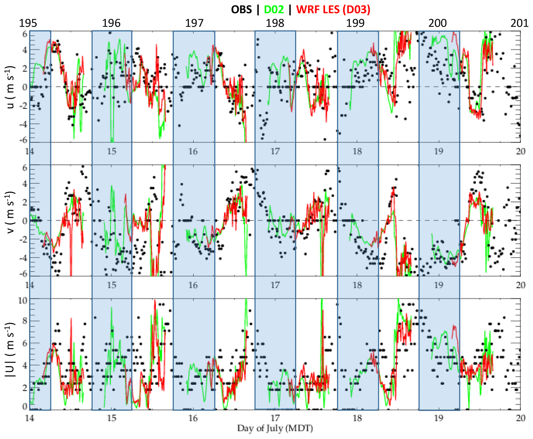
Figure 3 Comparison of predicted u wind component, v wind component and wind speed at 10 m a.g.l. obtained from WRF D02 and WRF LES forced with 04:00 UTC HRRR with observations (OBS) obtained from an AWOS surface meteorological station at Saguache Municipal Airport located at the base of Saguache Canyon. WRF-D02 data are instantaneous values while WRF LES data are 10 min averages. AWOS data from SAG are plotted when available (roughly every 15 min). Nighttime conditions are indicated by the blue regions (approximately 18:00 to 06:00 MDT). Day of year is indicated along the top. The location of the SAG AWOS station is marked with an “*” in Fig. 1.

Overall, the diurnal variability was captured quite well by both domains. Both D02 and D03 had very similar timing for the flow reversal from drainage to up-canyon winds between 08:00–10:00 MDT each day (Fig. 3). Because the larger-scale variability in WRF LES closely tracks that in D02, it is clear that the performance of WRF D02 was critical in properly initializing the drainage flow within the nested LES domain as well as in downscaling the HRRR data and driving the lateral boundaries of the WRF LES computational grid. It is noted that the onset of drainage flow winds always occurred prior to the 04:00 MDT initialization time of the D03. Additional simulations have been performed in archive mode to assess the onset of the drainage flow within the WRF LES (D03) domain and will be reported on in the future.

Throughout the 1-week period, the largest differences in the wind speed and direction between the two domains occurred during the daytime (Fig. 3). There are several stronger wind spikes evident in the D02 time series that are not evident within D03, with obvious daytime offsets occurring after noon local time on 19 July 2018. Further inspection revealed that these differences were associated with differences in the placement of moist convection and subsequent outflows within the two domains. Differences in the modeled evolution of the nighttime drainage flows obtained within the two domains are generally small except on 19 July 2018 when the westerly component is much stronger in D03 (note that the v component is more similar). Despite this initial offset between D02 and D03 initialization, the 10 m winds become very similar within about 2 h of the D03 initialization. Further analyses are ongoing to assess why there was such a large difference between D02 values and those used as initial conditions in D03 for this case.

While the predicted timing of stronger afternoon winds was not exact, the general trends toward gustiness in the afternoon were well-captured by both domains. On 17 July 2018, convection and associated outflow winds near the surface were predicted within both domains at SAG (Fig. 3). Surface observations (Fig. 3) indicate that stronger winds did develop in the afternoon in response to convective storms that were evident in the Pueblo NEXRAD reflectivity field (not shown). As observed, the model predicted winds to increase at SAG as convective storms over higher terrain produced outflows and propagated southward into the SLV (Fig. 4). Outflow winds exceeding 10 m s⁻¹ are predicted at several locations around the edges of the SLV including areas around Saguache and just west of the Sangre de Cristo Mountains (Fig. 4a). The leading edge of the outflow boundaries near Saguache are accompanied by enhanced upward motions (Fig. 4b). The outflows merged with thermals organized in hexagonal-like cells, which are still evident in areas that have yet to be disturbed by moist convection in the prediction. These predictions of a highly variable 3D wind field (strong winds, thermal updrafts and downdrafts exceeding 2 m s⁻¹) and the possibility of convective precipitation are all potential hazards to UAS safety and efficiency and, as such, would be critical information for support UAS flight planning and UAS traffic management (UTM).

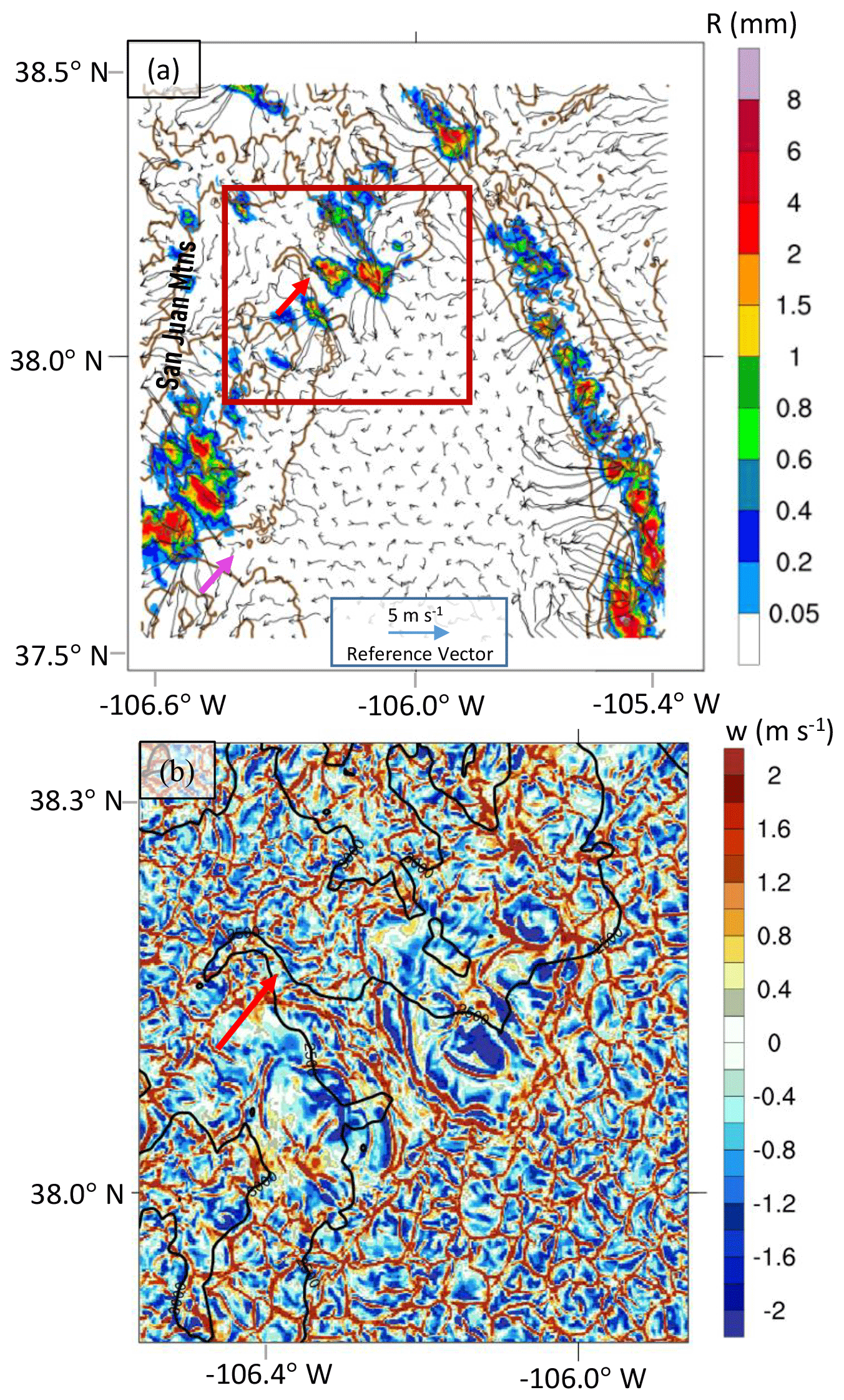
Figure 4 Simulated (a) 80 m winds (direction and magnitude) and 1 h precipitation accumulation (R, color contours) and (b) vertical velocities (w) at 180 m a.g.l. from WRF LES valid at 14:30 MDT on 17 July 2018. Region shown in panel (b) is a 40 km box outlined in panel (a) which is centered on SAG Airport. Terrain contours are also given for reference in both panels. Saguache Canyon is identified with the red arrow in panels (a) and (b), while Rio Grande Canyon is pointed out with the magenta arrow in panel (a).

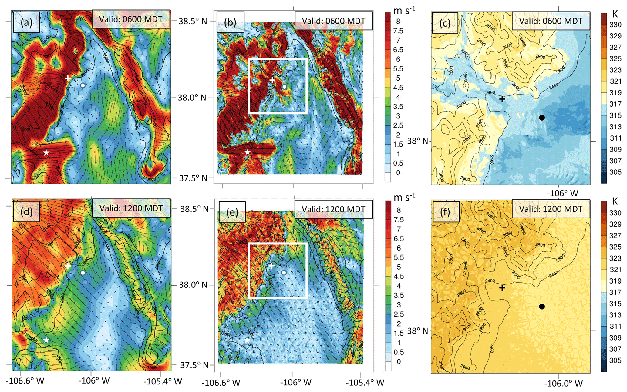
Figure 5 Wind speed (colors) and direction (arrows) at 80 m a.g.l. from (a) HRRR (issued at 22:00 MDT on previous day) and (b) WRF LES and (c) WRF LES potential temperature at 80 m a.g.l. for zoomed-in region denoted by the white box in panel (b) for forecasts valid at 06:00 and 12:00 MDT on 19 July 2018. Model terrain heights are denoted by black contours. Symbols denote locations as follows: asterisk – Saguache; star – Del Norte; filled circle – NSSL sounding site.

As mentioned above, drainage winds were observed at SAG before sunrise each day during LAPSE-RATE. A drainage flow IOP took place on 19 July 2018. Figure 3 indicates fairly strong ($\left|U\right|$ > 6 m s⁻¹) drainage winds were predicted at SAG within both D02 and D03. Comparison of the wind field obtained from the operational HRRR run with that obtained with WRF LES at 80 m a.g.l. reveals notable differences in the scales of variability resolved by the two models (Fig. 5). Larger-scale features are relatively similar between the two models. Both indicate persistent northwesterly flow at mountaintop perpendicular to the San Juan Mountains in the early morning (06:00 MDT) with weaker, generally southerly winds throughout the SLV. Both models also indicate the presence of drainage flow from the Rio Grande Canyon during the early morning but only the WRF LES shows drainage winds emanating from Saguache Canyon. In addition, the HRRR indicates stronger widespread (4–5 m s⁻¹) up-valley flow across much of the SLV during this time while the WRF LES indicates the presence of narrow channels of weaker (generally less than 3 m s⁻¹) up-valley flow. Finally, WRF LES indicates the presence of several smaller-scale (meso-gamma scale) circulations/eddies within the SLV that are not evident in the HRRR.

By 12:00 MDT, the patterns have diverged even further. The HRRR indicates that the persistent northwesterly winds near mountaintops have weakened, and winds within the SLV have rotated to upslope on both sides of the SLV with very weak winds in the center of the SLV (Fig. 5). The WRF LES maintains slightly stronger mountaintop winds with notably weaker and smaller-scale areas of upslope flow along the San Juan and Sangre de Cristo Mountains. The WRF LES also has generally weaker winds throughout the SLV at this time (< 2 m s⁻¹). WRF LES also depicts evidence of the convective PBL development, which results in a small-scale cellular pattern of locally enhanced low-level winds. The HRRR only depicts larger-scale variability with the strongest winds (5 m s⁻¹) along the foothills of the San Juan Mountains.

Drainage winds develop in response to horizontal pressure gradients that form via differential cooling of air within the canyon (and along the canyon walls) and cooling of air at the same height out over the valley. The potential temperature patterns evident in Fig. 5c reveal the cold drainage flow in Saguache Canyon resulting in sharp horizontal gradients along a terrain-following sigma level near roughly 80 m a.g.l. (note that the height of the sigma level varies slightly with x,y, and 80 m a.g.l. is the domain average value). By noon, it is clear that temperatures in the canyon have warmed faster than surrounding higher terrain, which results in local rising of air and a reversal of flow in the canyon to the southeast.

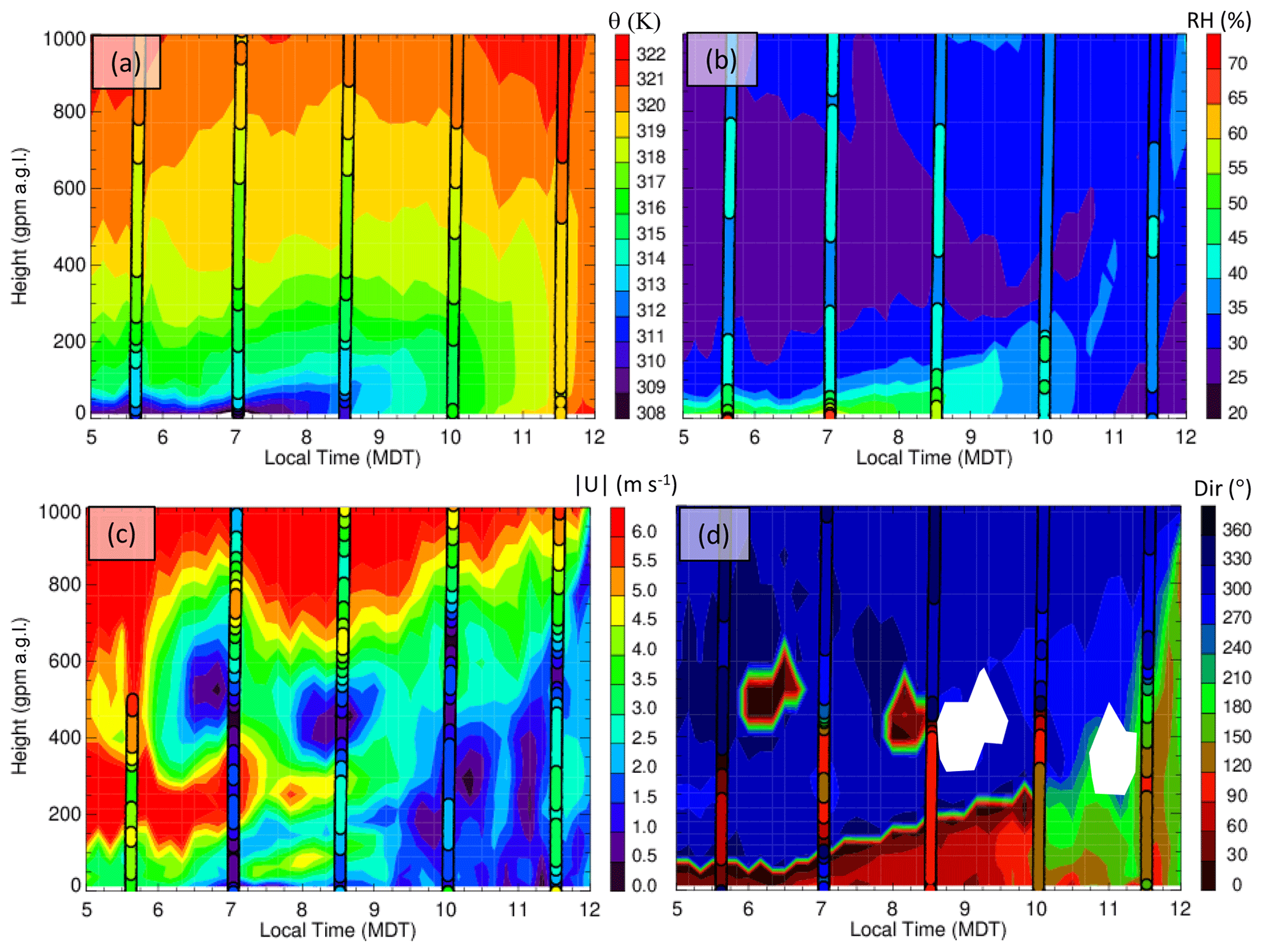
Figure 6 Time–height plots depicting WRF LES modeled evolution of the boundary layer during the drainage flow case observed on 19 July 2018 as evident in (a) potential temperature, (b) relative humidity, (c) wind speed and (d) wind direction. NSSL sounding data are overlaid within vertical columns corresponding with radiosonde launch times. Model data (with 10 min output frequency) are from innermost WRF LES grid at grid point closest to 38.05^∘ N, 160.05^∘ W. The location of the NSSL soundings on this day is shown in Fig. 1.

The modeled evolution of the cold pool that developed just outside the mouth of Saguache Canyon is assessed using observations from NSSL radiosondes (Fig. 6). Most of the NSSL soundings obtained on 19 July 2018 were collected roughly 11 km southeast of Saguache Municipal Airport (2393 m a.m.s.l.) with a surface elevation of 2313 m a.m.s.l. The five radiosondes that were launched at this location indicate that the cold pool was generally less than 100 m deep with a temperature deficit of 5 ^∘C. The WRF LES captures the strength of this shallow inversion layer fairly well. The modeled strength of the surface-based inversion is also readily apparent in the modeled temperature profile shown in Fig. 1 (red shows modeled temperature profile at NSSL site). Both the modeled and observed potential temperature profiles exhibit a weakly stable stratification above the surface-based inversion. The WRF LES also generally captures the timing of convective mixing between 08:30 and 12:00 MDT as is evident in the increasing depth of constant potential temperature (indicating the depth of the well-mixed layer). Thus, the simulation generally captures both the vertical structure and evolution of the stability for this case with only slight discrepancies in the stability just above the surface-based inversion.

The modeled moisture profile is also similar to that observed except for a notable dry bias near the surface. Biases of about 10 % are evident above the surface-based inversion layer. The large dry bias at the surface is potentially indicative of the surface boundary being too dry in the model. Future work could be performed to assess whether improving the lower-boundary condition improves the forecasts.

In terms of winds, both the soundings and WRF LES data indicate significant vertical shear and temporal variability in winds within the lowest 1 km of the atmosphere. NSSL sounding data reveal that winds below 400 m are generally light and from the east-southeast prior to sunrise with stronger northwesterlies above 500 m a.g.l. This is in contrast to observations at SAG where low-level winds are from the northwest at 5 m s⁻¹ prior to sunrise (Fig. 3). The 07:00 MDT sounding detects weak northwesterly flow below 100 m, which indicates that drainage winds may have briefly extended to the NSSL sounding site. The WRF LES data indicate the presence of much stronger and elevated drainage winds at the NSSL launch site between 05:00 and 08:30 MDT (decreasing with time after 07:15 MDT) with low-level jet core winds exceeding 6 m s⁻¹ between 150 and 400 m a.g.l. (much stronger than any winds that were observed below 1 km a.g.l.).

Examination of the spatial extent of the drainage flow in the WRF LES simulation indicates the presence of sharp gradients in the modeled strength and extent of northwesterly winds (Fig. 5b). Thus, small offsets in the modeled position of the drainage flow can result in significant model error when point-based comparisons are made. In addition, evidence presented by Jensen et al. (2021) demonstrates sensitivity of the modeled drainage flow to initial conditions. They found that assimilating UAS observations generally improved the simulated evolution, strength and timing of the drainage flow and subsequent flow reversal. Despite biases in the simulated drainage flow, both the WRF LES and NSSL soundings indicate that east-southeast winds deepen with time after sunrise in response to daytime heating with sunrise being at 06:30 MDT (Fig. 6d).

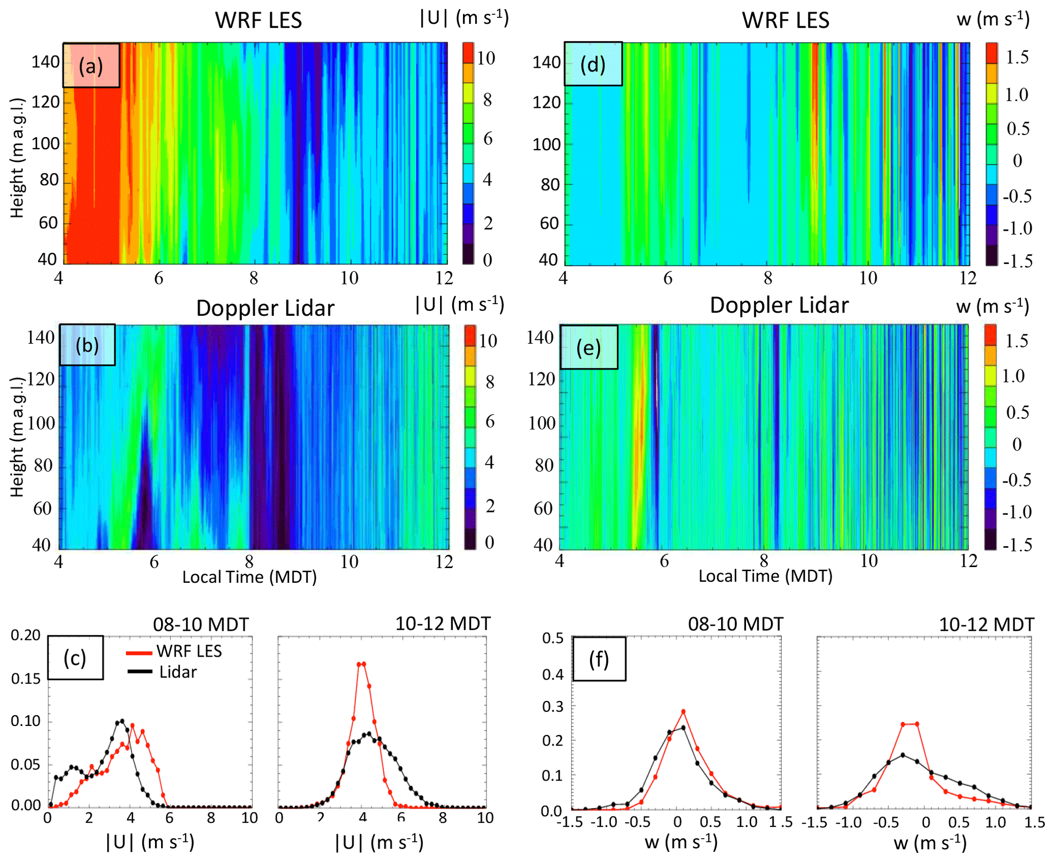
Figure 7 Time–height plots depicting evolution of wind speed and vertical velocity from (a, d) WRF LES and (b, e) University of Colorado Doppler lidar at Saguache Municipal Airport on 19 July 2018. The bottom row of plots provides distributions of (c) wind speed and (f) vertical velocity from WRF LES (red) and Doppler lidar (black) using 10 s data for two time periods (08:00–10:00 and 10:00–12:00 MDT) using all samples obtained between 40 and 140 m a.g.l.

A key aspect of the WRF LES simulations is the ability to explicitly resolve convective boundary layer structures (Nolan et al., 2018) and meso-gamma-scale flows described above. Examination of the drainage flow case indicates that the WRF LES also had skill in predicting finer-scale variations in the winds and characteristics of turbulence as the boundary layer transitioned from nocturnal to convective in complex terrain. As evident in the predicted surface winds (Fig. 3), the strength of the drainage flow was over-predicted on 19 July 2018. This bias is evident as a deep layer of strong winds in WRF LES that initially exceed 10 m s⁻¹ through the lower atmosphere (Fig. 7a). This bias is related to biases in the initial conditions and boundary conditions provided by D01. Lidar observations indicate the presence of a much shorter-lived drainage flow with a weaker peak wind (peak value ∼ 6 m s⁻¹) that undulates between the lowest range gate and 140 m a.g.l. between 05:00 and 07:00 MDT (Fig. 7b). Interestingly, the WRF LES demonstrates a similar, albeit slightly later, undulation with stronger winds between 06:00 and 08:00 MDT. Generally, the winds predicted by WRF LES come into better agreement with the Doppler lidar observations with time as local processes begin to dominate and the impact of the poor initial conditions begins to wane.

Comparison of the turbulent properties of the flow reveals some interesting features as well. Here we focus on the morning transition which is characterized by PBL growth and transition to up-canyon flow, which was observed to commence at 08:00 MDT. This transition to up-valley flow is indicated by the sharp change in wind speed in the Doppler lidar data (Fig. 7b) which is consistent with the 10 m wind observations (Fig. 3). The predicted shift to up-valley flow occurs about 45 min late (Fig. 7a). Comparisons of wind speed and vertical velocity distributions for mid-morning and late morning are shown in Fig. 7c, f. As expected, the distribution of wind speeds and vertical velocities changes throughout the morning with both modeled and observed distributions broadening with time. The observed distributions of the 08:00–10:00 MDT wind speed and vertical velocity are well-captured by the model. The biases in the wind speeds for this time period are due to over-prediction of the drainage flow strength and duration. By late morning, the modeled distributions for wind speed and vertical velocity are too peaked, indicating a delay in the modeled development of the convective boundary layer. The potential cause of the delay in simulated turbulence is currently under investigation.

4 Description of model dataset

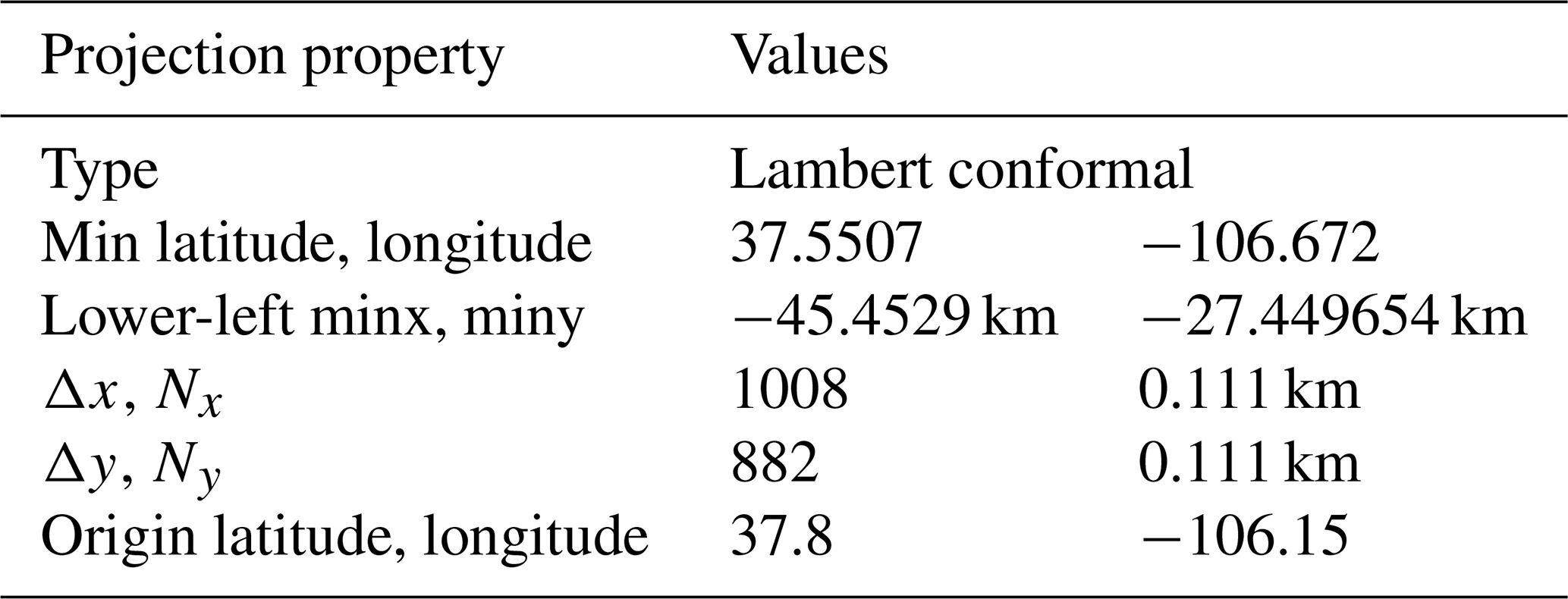
Data from the real-time WRF modeling system were post-processed using a modified Version 3 of the UPP. The UPP was extended to handle sub-hourly output and to add additional diagnostic outputs like TKE at flight levels. The UPP was also used to de-stagger the mass and wind field grids onto a single common grid, rotate the horizontal wind vectors from grid-relative to earth-relative frame of reference, interpolate from computational hybrid levels to heights above ground level (i.e., flight levels) and compute a number of diagnostics (Table 2). A detailed description of the UPP V3.0 is available online. The grids were output every 10 min for both domains (D02 and D03). The UPP was also used to convert the data from the raw WRF netCDF format to standard WMO Grib2 data format. Specifics describing the grid projection are given in Table 3.

Table 2 Description of gridded output variables in Grib2 format.

^∗ Level codes: 1: surface; 3: visibility at surface; 100: lowest 400 hPA; 103: profile (height a.g.l.); 104: layer mean value; 200: column; 215: cloud ceiling height.

Table 3 Projection information for Grib2 for WRF LES grid (D03).

The file naming convention follows

WRFPRS_YYYYMMDDhhmm_dnn.lh_lm

where

• YYYYMMDD is the date the model run was initialized in UTC,

• hhmm is the hour and minute of the day that the model run was initialized in UTC,

• nn is domain number (01,02 – for 04:00 UTC runs or 02,03 – for 18:00 UTC runs),

• lh is forecast outlook hour,

• lm is forecast outlook min,

• valid_time is hhmm plus lhlm.

Additional data were output in ASCII format at three locations (i.e., Saguache Municipal Airport, Moffat and Leach Airport) where observational systems (both surface-based and UAS) were located during LAPSE-RATE. The ASCII output files contain model data fields at a frequency determined by the time step used to integrate the equations of motion within that domain (D02: 6 s, D03: 0.666 s). The files are stored using the following naming convention:

XXX.dnn.ZZ.yyyymmddhh.gz

where XXX is the location name (SAG – Saguache, MOF – Moffat, LEA – Leach), nn is the domain number (02 – for 04:00 UTC runs or 03 – for 18:00 UTC runs), ZZ is the variable and yyyymmddhh is the model initialization time (UTC).

Table 4 Description of variables stored for point locations in ASCII format.

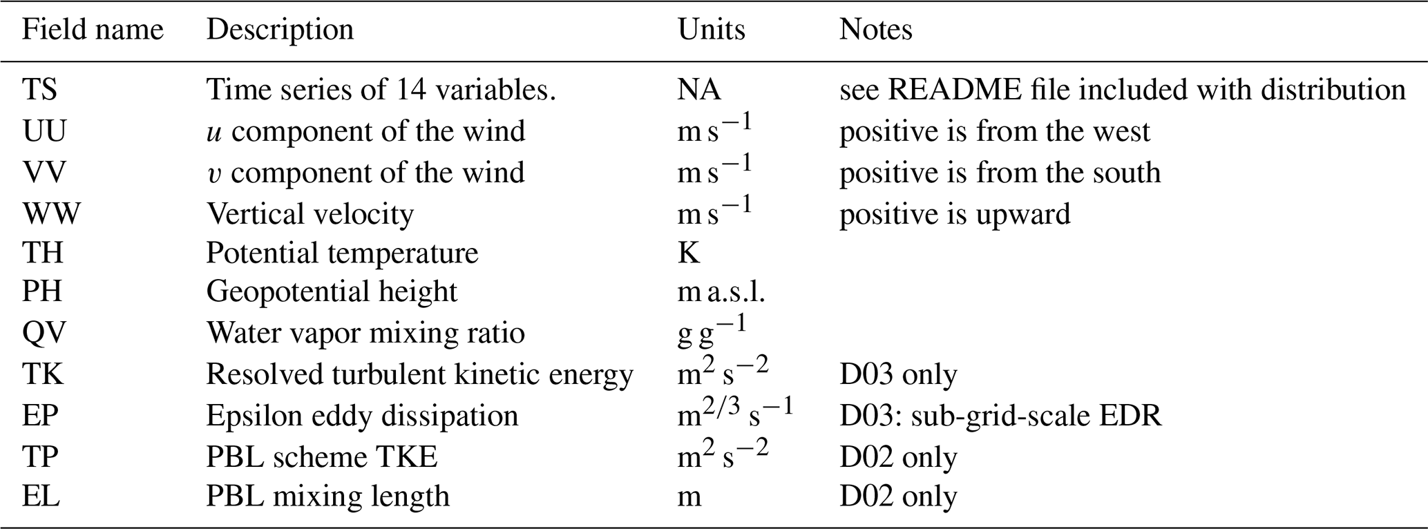
These ASCII files are formatted to provide time series of profiles up to 1850 m a.g.l. (where VV is “PH”, “QV”, “TH”, “UU”, “VV”, “WW”, “TK”, “TP”, “EL”, “EP”) and time series of surface meteorological data, vertically integrated quantities and stability parameters (ZZ is “TS”). The value and units for each ZZ variable are given in Table 4. The format of the profile time series files is such that after the file header row, each subsequent row (or data record) includes the forecast lead time (LT) and values of the given variable for the lowest 25 model levels. The valid time in UTC is equal to hh + LT. Details of the format of the `TS' files, which contains 19 variables per row, are given in the README file that accompanies the dataset.

5 Data availability

An overview of all of the LAPSE-RATE datasets that have been archived is given by de Boer et al. (2020b, https://zenodo.org/communities/lapse-rate/, last access: 1 December 2020). Because of the size of the model files, in particular the 3D grids, only the time series ASCII data files and samples of the 3D model grids are provided at https://zenodo.org/record/3706365#.X8VwZrd7mpo (Pinto et al., 2020b). The full set of model grids and time series files can be obtained from the NCAR's Digital Asset Services Hub (DASH) repository at https://doi.org/10.5065/83r2-0579 (Pinto et al., 2020a). In addition, raw model data that have not been post-processed (i.e., not de-staggered, hybrid levels and stored in WRF netCDF format) are available upon direct request to the corresponding author.

6 Summary

Microscale real-time simulations were conducted to support both next-day IOP planning and day-of UAS flight operations during LAPSE-RATE. Key components of this dataset are that they were generated using a nested configuration that enabled M2M coupling in which operational forecasts from both the GFS and the HRRR model were used to drive a nested WRF model configured such that the innermost domain was run at LES-permitting horizontal grid spacing of 111.11 m producing twice-per-day microscale predictions of a suite of variables for regions characterized by arid conditions and complex terrain. The data were processed on-the-fly using the UPP to store the output in operationally compatible standard Grib2 data format. Special fields were computed to support UAS operations including cloud ceiling height, radar reflectivity (used to diagnose convective hazards), visibility and turbulence intensity. The temperature and 3D velocity field generated with the WRF LES also contained relevant information with regard to the presence and intensity of thermals, the boundary layer depth and the presence of realistic boundary layer structures in the fine-scale predictions (Nolan et al., 2018).

Initial comparisons between model data and observations indicate that the model generally captured the meso-gamma-scale flows that characterized the low-level winds in the SLV during LAPSE-RATE. Conditions that were simulated over the course of the experiment include nocturnal terrain-driven flows, valley flows, convective boundary layer evolution, turbulence structures including hexagonal open cells, transitions from stable to convective PBL to moist deep convection and development of outflows. The wealth of observations collected by a number of small UASs and many ancillary platforms deployed during LAPSE-RATE will be a great asset for both evaluating fine-scale weather prediction models and assessing the value of UAS data assimilation in data-sparse regions and complex terrain (e.g., Jensen et al., 2021).