Greenland ice sheet mass balance from 1840 through next week

The mass of the Greenland ice sheet is declining as mass gain from snow accumulation is exceeded by mass loss from surface meltwater runoff, marine-terminating glacier calving and submarine melting, and basal melting. Here we use the input–output (IO) method to estimate mass change from 1840 through next week. Surface mass balance (SMB) gains and losses come from a semi-empirical SMB model from 1840 through 1985 and three regional climate models (RCMs; HIRHAM/HARMONIE, Modèle Atmosphérique Régional – MAR, and RACMO – Regional Atmospheric Climate MOdel) from 1986 through next week. Additional non-SMB losses come from a marine-terminating glacier ice discharge product and a basal mass balance model. From these products we provide an annual estimate of Greenland ice sheet mass balance from 1840 through 1985 and a daily estimate at sector and region scale from 1986 through next week. This product updates daily and is the first IO product to include the basal mass balance which is a source of an additional ∼24 Gt yr⁻¹ of mass loss. Our results demonstrate an accelerating ice-sheet-scale mass loss and general agreement (coefficient of determination, r², ranges from 0.62 to 0.94) among six other products, including gravitational, volume, and other IO mass balance estimates. Results from this study are available at https://doi.org/10.22008/FK2/OHI23Z (Mankoff et al., 2021).

1 Introduction

Over the past several decades, mass loss from the Greenland ice sheet has increased (Khan et al., 2015; IMBIE Team, 2019). Different processes dominate the regional mass loss of the ice sheet, and their relative contribution has fluctuated in time (Mouginot and Rignot, 2019). For example, in the 1970s nearly all sectors gained mass due to positive surface mass balance (SMB), except the northwestern sector, where discharge losses dominated. More recently, in the 2010s, all sectors lost mass, with some sectors losing mass almost entirely via negative SMB and others primarily due to discharge (Fig. 1).

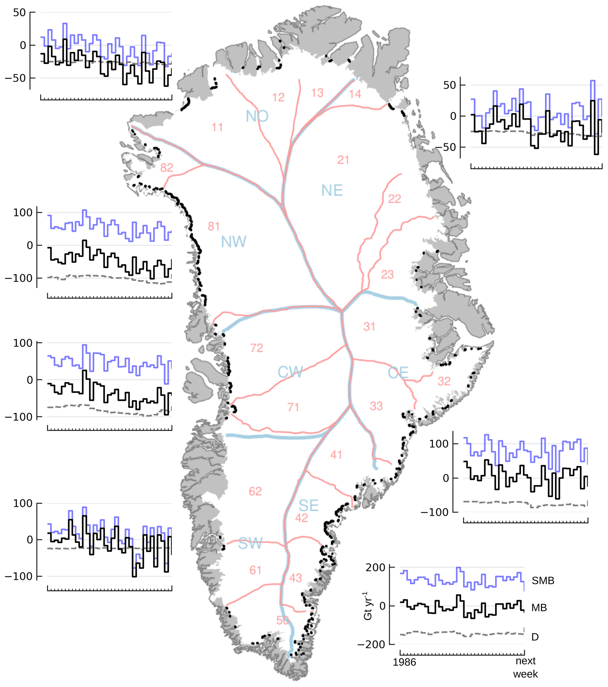
Figure 1 Annual mass balance (black lines), surface mass balance (blue lines), and discharge plus basal mass balance (dashed grey) in Gt yr⁻¹ for each of the seven Mouginot and Rignot (2019) regions. The map shows both the named regions (Mouginot and Rignot, 2019) and the numbered sectors (Zwally et al., 2012). Discharge gates are marked in black. Only recent (post-1986) data are shown because reconstructed data are not separated into regions or sectors. Next week is defined as 1 November 2021 based on the date this document was compiled.

There are three common methods for estimating mass balance – changes in gravity (Barletta et al., 2013; Groh et al., 2019; IMBIE Team, 2019; Velicogna et al., 2020), changes in volume (Simonsen et al., 2021a; Sørensen et al., 2011; Zwally and Giovinetto, 2011; Sasgen et al., 2012; Smith et al., 2020), and the input–output (IO) method (Colgan et al., 2019; Mouginot et al., 2019; Rignot et al., 2019; King et al., 2020). Each provides some estimate of where, when, and how the mass is lost or gained, and each method has some limitations. The gravity mass balance (GMB) estimate has low ∼100 km spatial resolution (where), monthly temporal resolution (when), and little information on the processes contributing to changes in mass balance components (how). The volume change (VC) mass balance estimate has ∼1 km spatial resolution (where), often provided at annual or multi-year temporal resolution (when), and little information on the driving processes (how).

The IO method has a complex spatial resolution (where). The inputs typically come from regional climate models (RCMs) which can reach a spatial resolution of up to 1 km. However, that spatial resolution is generally reduced in the final output to sector or region scale – typically higher than GMB but now lower resolution than VC. The IO temporal resolution (when) is limited by ice velocity data updates, which for the past several years occur every 12 d year-round after the launch of the Sentinel missions (Solgaard et al., 2021). The primary issue with the IO method is unknown ice thickness in some locations (e.g., Mankoff et al., 2020b). Finally, the IO method can provide insight into the processes (how) by distinguishing between changes caused by SMB (which may be due to changes in positive and/or negative SMB components) vs. changes in other mass loss terms (e.g., calving). Our IO method is also the first IO product to include the basal mass balance (Karlsson et al., 2021) – a term implicitly included in the GMB and VC methods but neglected by all previous IO estimates.

In this work we introduce the new Programme for Monitoring of the Greenland ice sheet (PROMICE) Greenland ice sheet mass balance data set based on the IO method, updating the previous product from Colgan et al. (2019). We use the SMB field from one empirical model from 1840 through 1985 and three RCMs from 1986 onward. The combined SMB field used here is comprised of positive SMB terms (precipitation in the form of snowfall, rainfall, condensation/riming, and snow drift deposition) and negative SMB terms (surface melt, evaporation, sublimation, and snow drift erosion). We also use the basal mass balance and an estimate of dynamic ice discharge. Spatial resolution is effectively per sector (Zwally et al., 2012) or region (Mouginot and Rignot, 2019). Temporal resolution is annual from 1840 through 1985 and effectively daily since 1986 – the RCM fields are updated daily and forecasted through next week, and the discharge at marine-terminating glaciers is updated every 12 d with ∼12 d resolution, interpolated to daily, and forecasted using historical and seasonal trends through next week. Thus, this study provides a daily-updating estimate of Greenland mass changes from 1840 through next week.

2 Terminology

We use the following terminology throughout the document.

• This Study refers to the new results presented in this study.

• Recent refers to the new 1986 through next week daily temporal resolution data at regional and sector scales.

• Reconstructed refers to the adjusted Kjeldsen et al. (2015) annual temporal resolution data at ice sheet scale used to extend this product from 1986 back through 1840. The 1986 through 2012 portion of the Kjeldsen et al. (2015) data set is used only to adjust the reconstructed data and is then discarded.

• ROI (region of interest) refers to one or more of the ice sheet sectors or regions (Fig. 1).

• Sector refers to one of the Zwally et al. (2012) sectors (Fig. 1), expanded here to cover the RCM ice domains which exist slightly outside these sectors in some locations.

• Region refers to the Mouginot and Rignot (2019) regions (Fig. 1), expanded here to cover the RCM ice domains.

• SMB is the surface mass balance from an RCM or the average of multiple RCM SMBs. The use should be clear from the context.

• D is solid ice discharge. It includes both calving and submarine melting at marine-terminating glaciers.

• BMB is the basal mass balance. It comes from geothermal flux (BMB_GF), frictional heating from ice velocity (BMB_friction), and viscous heat dissipation (BMB_VHD).

• MB is the total mass balance including the BMB term (Eq. 3).

• MB^* is the mass balance not including the BMB term (Eq. 4).

• HIRHAM/HARMONIE, Modèle Atmosphérique Régional (MAR), and Regional Atmospheric Climate MOdel (RACMO) refer to the RCMs, which only provide SMB and runoff in the case of MAR. However, when referencing the different MB products, we use, for example, “MAR MB” rather than repeatedly explicitly stating “MB derived from MAR SMB minus BMB and D”. The use should be clear from the context.

3 Product description

The output of this work is two NetCDF files and two CSV files containing a time series of mass balance and the components used to calculate mass balance. The only difference between the two NetCDF files is the region of interest (ROI) – one for Zwally et al. (2012) sectors and one for Mouginot and Rignot (2019) regions. Each NetCDF file includes the ice sheet mass balance (MB), MB per ROI (sector or region), MB per ROI per RCM, ice sheet SMB, SMB per ROI, ice sheet discharge (D), D per ROI, ice sheet BMB, and BMB per ROI. The CSV files contain a copy of the ice-sheet-summed data, one daily and one annual.

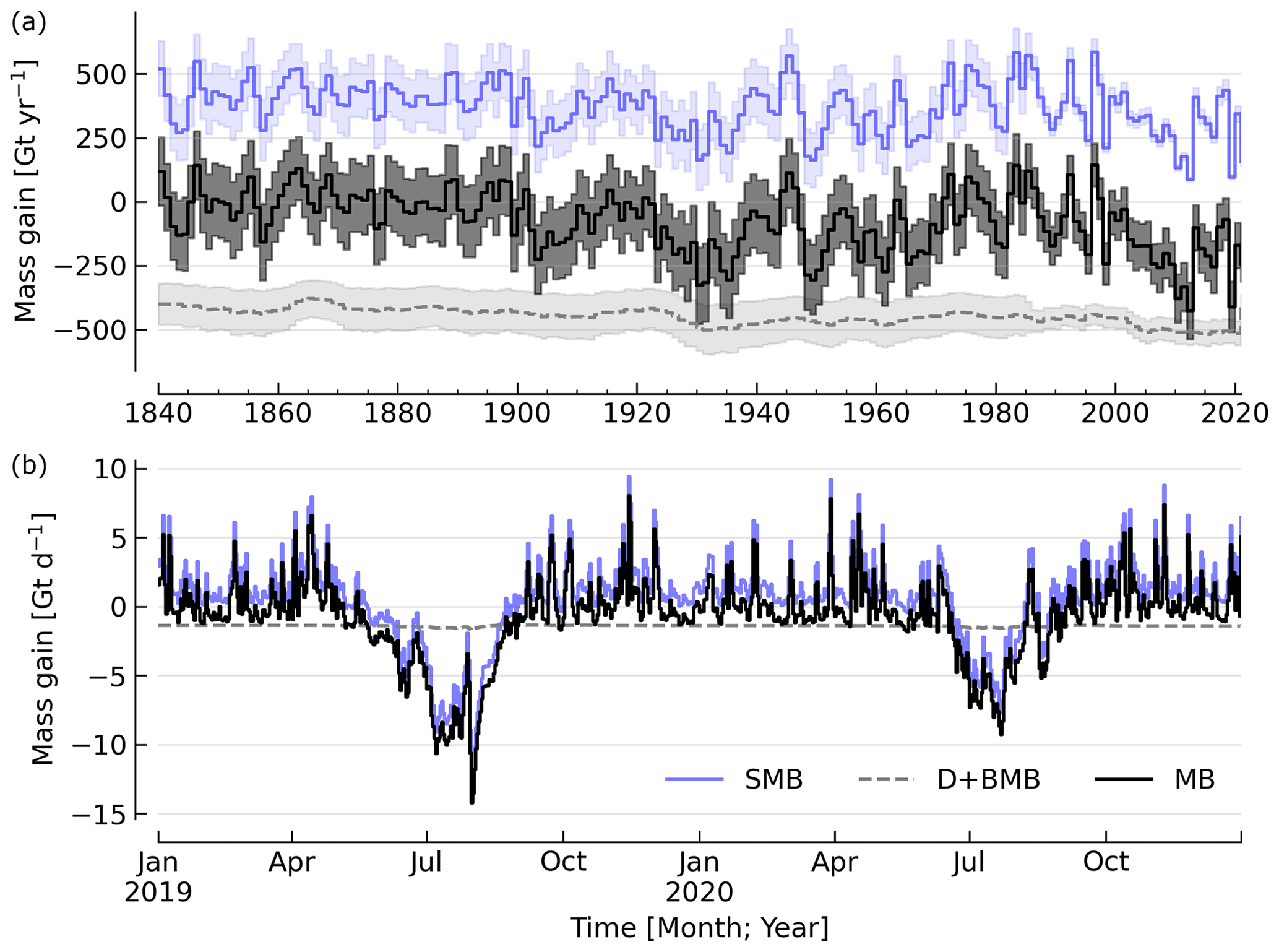
Figure 2 Mass balance and its major components. (a) Annual average surface mass balance (blue line), discharge (gray dashed), and their mass balance sum (black line). Here the discharge and basal mass balance (D + BMB) are shown with sign inverted (e.g., $-\mathrm{1}\times (\mathrm{D}+\text{BMB})$). (b) Same data at daily resolution and limited to 2019 and 2020.

An example of the output is shown in Fig. 2a, which shows mass balance for the entire Greenland ice sheet in addition to SMB and D at annual resolution. Figure 2b shows an example of 2 years at daily temporal resolution. The ice-sheet-wide product includes data from 1840 through next week, but the sector and region-scale products only include data from 1986 through next week, because the 1840 through 1985 reconstructed only exists at ice sheet scale (Fig. 1).

4 Data sources

This section introduces data products that exist prior to and are external to this work (Table 1). In the following Methods section we introduce both the intermediate products we generate using these data sources and the final product that is the output of This Study.

Kjeldsen et al. (2015)Box et al. (2021)Kjeldsen et al. (2015)Box et al. (2021)Langen et al. (2017)Fettweis et al. (2020)Noël et al. (2019)Mankoff et al. (2020b)Mankoff and Solgaard (2020)Karlsson et al. (2021)Karlsson (2021)Kjeldsen et al. (2015)Box et al. (2021)Fettweis et al. (2020)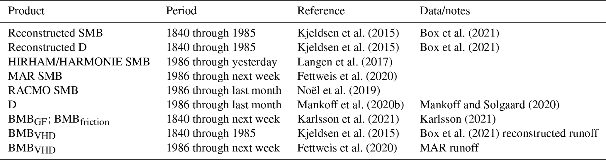

Table 1 Summary of data products used as inputs to This Study.

The inputs to this work are the recent SMB fields from the three RCMs, the recent discharge from Mankoff et al. (2020b) (data: Mankoff and Solgaard, 2020), and the recent basal mass balance fields, of which BMB_GF and BMB_friction are direct outputs from Karlsson et al. (2021) (data: Karlsson, 2021), but the BMB_VHD calculations are redone here (see Methods Sect. 5.3) using the MAR runoff field. The reconstructed data (pre-1986) are surface mass balance and discharge from Kjeldsen et al. (2015) (data: Box et al., 2021) but adjusted here using the overlapping period (see Methods Sect. 5.4) and runoff from Kjeldsen et al. (2015) (data: Box et al., 2021) as a proxy and scaled for BMB_VHD (see Methods Sect. 5.3).

4.1 Surface mass balance

We use one reconstructed SMB from 1840 through 1985 and three recent SMBs from 1986 through last month (HIRHAM/HARMONIE, MAR, and RACMO), two through yesterday (HIRHAM/HARMONIE and MAR) and one through next week (MAR).

4.1.1 HIRHAM/HARMONIE

The HIRHAM/HARMONIE product from the Danmarks Meteorologiske Institut (Danish Meteorological Institute; DMI) is based on an offline subsurface firn/SMB model (Langen et al., 2017), which is forced with surface fluxes of energy (turbulent and downward-radiative) and mass (snow, rain, evaporation, and sublimation). These surface fluxes are derived from the HIRHAM5 regional climate model for the reconstructed part of the simulation and from DMI's operational numerical weather forecast model HARMONIE (Iceland–Greenland domain “B”, which covers Iceland, Greenland, and the adjacent seas) for the real-time part. HIRHAM5 is used until 31 August 2017, after which HARMONIE is used.

The HIRHAM5 regional climate model (Christensen et al., 2007) combines the dynamical core of the HIRLAM7 numerical weather forecasting model (Eerola, 2006) with physics schemes from the ECHAM5 general circulation model (Roeckner et al., 2003). In the Greenland setup employed here (Lucas-Picher et al., 2012), it has a horizontal resolution of $\mathrm{0.05}{}^{\circ }\times \mathrm{0.05}$^∘ on a rotated pole grid (corresponding to 5.5 km resolution) and 31 atmospheric levels. It is forced at 6 h intervals on the lateral boundaries with horizontal wind vectors, temperature, and specific humidity from the ERA-Interim reanalysis (Dee et al., 2011). ERA-Interim sea surface temperatures and sea ice concentration are prescribed in ocean grid points. Surface fluxes from HIRHAM5 are passed to the offline subsurface model.

The offline subsurface model was developed to improve firn details for the HIRHAM5 experiments (Langen et al., 2017). The subsurface consists of 32 layers with time-varying fractions of snow, ice, and liquid water. Layer thicknesses increase with depth from 6.5 cm water equivalent (w.e.) at the top to 9.2 m w.e. at the bottom, giving a full model depth of 60 m w.e. The processes governing the firn evolution include snow densification, varying hydraulic conductivity, irreducible water saturation and other effects on snow liquid water percolation, and retention. Runoff is calculated from liquid water in excess of the irreducible saturation with a characteristic local timescale that depends on surface slope (Zuo and Oerlemans, 1996; Lefebre, 2003). The offline subsurface model is run on the HIRHAM5 5.5 km grid.

HARMONIE (Bengtsson et al., 2017) is a nonhydrostatic model in terrain-following sigma coordinates based on the fully compressible Euler equations (Simmons and Burridge, 1981; Laprise, 1992). HARMONIE is run at 2.5 km horizontal resolution and with 65 vertical levels. Compared to previous model versions, upper-air 3D variational data assimilation of satellite wind and radiance data, and radio occultation data, radiosonde, aircraft, and surface observations are incorporated. This greatly improves the number of observations in the model, as in situ observations from ground stations and radiosondes only make up approximately 20 % of observations in Greenland (Wang and Randriamampianina, 2021; Yang et al., 2018). The model is driven at the boundaries with European Centre for Medium-Range Weather Forecasts (ECMWF) high-resolution data at 9 km resolution. The 2.5 km HARMONIE output is regridded to the 5.5 km HIRHAM grid before input to the offline subsurface model. The HIRHAM5 and offline models both employ the Citterio and Ahlstrøm (2013) ice mask interpolated to the 5.5 km grid.

4.1.2 MAR

The MAR RCM has been developed by the University of Liège (Belgium) with a focus on the polar regions (Fettweis et al., 2020). The MAR atmosphere module (Gallée and Schayes, 1994) is fully coupled with the soil–ice–snow energy balance vegetation model SISVAT (Gallée et al., 2001) simulating the evolution of the first 30 m of snow or ice over the ice sheet with the help of 30 snow layers (with time-varying thickness) or the first 10 m of soil over the tundra area. At its lateral boundary, MAR is forced at 6 h intervals by ERA5 reanalysis and runs at 20 km resolution. The snowpack was initialized in 1950 from a former MARv3.11-based simulation. Its snow model is based on a former version of the CROCUS snow model (Vionnet et al., 2012) dealing with all the snowpack processes, including the meltwater retention, transformation of melting snow and grain size, compaction of snow, formation of ice lenses impacting meltwater penetration, warming of the snowpack from rainfall, and complex snow/bare ice albedo. MAR uses the Greenland Ice Mapping Project (GIMP) ice sheet mask and ice sheet topography (Howat et al., 2014).

We use MAR version 3.12. With respect to version 3.9, intensively validated over Greenland (Fettweis et al., 2020), or the 20 km-based MARv3.10 setup used in Tedesco and Fettweis (2020), MARv3.12 now uses the common polar stereographic projection EPSG 3413. With respect to MARv3.11, fully described in Amory et al. (2021), MARv3.12 ensures now the full conservation of water mass into both soil and snowpack at each time step, takes into account the geographical projection deformations in its advection scheme, better deals with the snow/rain temperature limit with a continuous temperature threshold between 0 and −2 ^∘C, increases the evaporation above snow thanks to a saturated humidity computation in SISVAT adapted to freezing temperatures, disallows melt below the 30 m of the resolved snowpack, and includes small improvements and bug fixes with the aim of improving the evaluation of MAR (with both in situ and satellite products) as presented in Fettweis et al. (2020) in addition to small computer time improvements in the parallelization of its code.

In addition to providing SMB, MAR also provides daily runoff over both permanent ice and tundra area. The ice runoff is used for the daily BMB_VHD estimate (Sect. 5.3).

As the recent SMB decrease (successfully evaluated with GRACE-based estimates in Fettweis et al., 2020) has been fully driven by the increase in runoff (Sasgen et al., 2020), we assume the same degree of accuracy between SMB simulated by MAR (evaluated with the PROMICE SMB database in Fettweis et al., 2020) and the runoff simulated by MAR.

Weather-forecasted SMB. To provide a real-time state of the Greenland ice sheet, MAR is forced automatically every day by the run of 00:00 UTC from the Global Forecast System (GFS) model providing weather forecasting initialized by the snowpack behaviors of the MAR run from the previous day. This continuous GFS-forced time series (without any reinitialization of MAR) provides SMB and runoff estimates between the period covered by ERA5 and the next 7 d. At the end of each day, ERA5 is used to update the GFS-forced MAR time series until about 5 d before the current date and to provide a homogeneous ERA5-forced MAR times series from 1950 to a few days before the current date. We use both the forecasted SMB and forecasted runoff (for BMB_VHD) fields.

4.1.3 RACMO

RACMO v2.3p2 has been developed at the Koninklijk Nederlands Meteorologisch Instituut (Royal Netherlands Meteorological Institute; KNMI). It incorporates the dynamical core of the High-Resolution Limited Area Model (HIRLAM) and the physics parameterizations of the ECMWF Integrated Forecast System cycle CY33r1. A polar version (p) of RACMO has been developed at the Institute for Marine and Atmospheric research of Utrecht University (UU-IMAU) to assess the surface mass balance of glaciated surfaces. The current version RACMO2.3p2 has been described in detail in Noël et al. (2018), and here we repeat the main characteristics.

The ice sheet has an extensive dry interior snow zone, a relatively narrow runoff zone along the low-lying margins, and a percolation zone of varying width in between. To capture these processes on first order, the original single-layer snow model in RACMO has been replaced by a 40-layer snow scheme that includes expressions for dry snow densification and a simple tipping bucket scheme to simulate meltwater percolation, retention, refreezing, and runoff (Ettema et al., 2010). The snow layers were initialized in September 1957 using temperature and density from a previous run with the offline IMAU Firn Densification Model (Ligtenberg et al., 2018). To simulate drifting snow transport and sublimation, Lenaerts et al. (2012) implemented a drifting snow scheme. Snow albedo depends on snow grain size, cloud optical thickness, solar zenith angle, and impurity content (van Angelen et al., 2012). Bare ice albedo is assumed constant and estimated as the 5th percentile value of albedo time series (2000–2015) from the 500 m-resolution MODIS 16 d albedo product (MCD43A3). Minimum/maximum values of $\mathrm{0.30}/\mathrm{0.55}$ are applied to the bare ice albedo, representing ice with high-/low-impurity content (cryoconite, algae).

To simulate as accurately as possible the contemporary climate and surface mass balance of the ice sheet, the following boundary conditions have been applied. The glacier ice mask and surface topography have been downsampled from the 90 m-resolution Greenland Ice Mapping Project (GIMP) digital elevation model (DEM) (Howat et al., 2014). At the lateral boundaries, model temperature, specific humidity, pressure, and horizontal wind components at the 40 vertical model levels are relaxed towards 6-hourly ECMWF reanalysis (ERA) data. For this we use ERA-40 between 1958 and 1978 (Uppala et al., 2005), ERA-Interim between 1979 and 1989 (Dee et al., 2011), and ERA-5 between 1990 and 2020 (Hersbach et al., 2020). The relaxation zone is 24 grid cells (∼130 km) wide to ensure a smooth transition to the domain interior. This run has active upper-atmosphere relaxation (van de Berg and Medley, 2016). Over glaciated grid points, surface aerodynamic roughness is assumed constant for snow (1 mm) and ice (5 mm). In this run, RACMO2.3p2 has 5.5 km horizontal resolution over Greenland and the adjacent oceans and land masses, but it was found previously that this is insufficient to resolve the many narrow outlet glaciers. The 5.5 km product is therefore statistically downscaled onto a 1 km grid sampled from the GIMP DEM (Noël et al., 2019), employing corrections for biases in elevation and bare ice albedo using a MODIS albedo product at 1 km resolution (Noël et al., 2016).

4.1.4 Reconstruction

The Kjeldsen et al. (2015) 173-year (1840 through 2012) mass balance reconstruction is based on the Box (2013) 171-year (1840 through 2010) statistical reconstruction. Kjeldsen et al. (2015) add a more sophisticated meltwater retention scheme (Pfeffer et al., 1991), weighting of in situ records in their contribution to the estimated value, and dispersal of annual accumulation to monthly and extend the reconstruction in time through 2012.

The Box (2013) 171-year (1840–2010) reconstruction is developed from linear regression parameters that describe the least squares regression between (a) spatially discontinuous in situ monthly air temperature records (Cappelen et al., 2011, 2006; Cappelen, 2001; Vinther et al., 2006) or firn/ice cores (Box et al., 2013) and (b) spatially continuous outputs from the regional climate model RACMO version 2.1 (Ettema et al., 2010). A 43-year overlap period (1960 through 2012) with the RACMO data is used to determine regression parameters (slope, intercept) on a 5 km grid cell basis. Temperature data define melting degree days, which have a different coefficient for bare ice than snow cover, determined from hydrological-year cumulative SMB. A fundamental assumption is that the calibration factors, regression slope, and offset for the calibration period 1960 through 2012 are stationary over time, for which there is some evidence in Fettweis et al. (2017). Box et al. (2013) describe the methods in more detail.

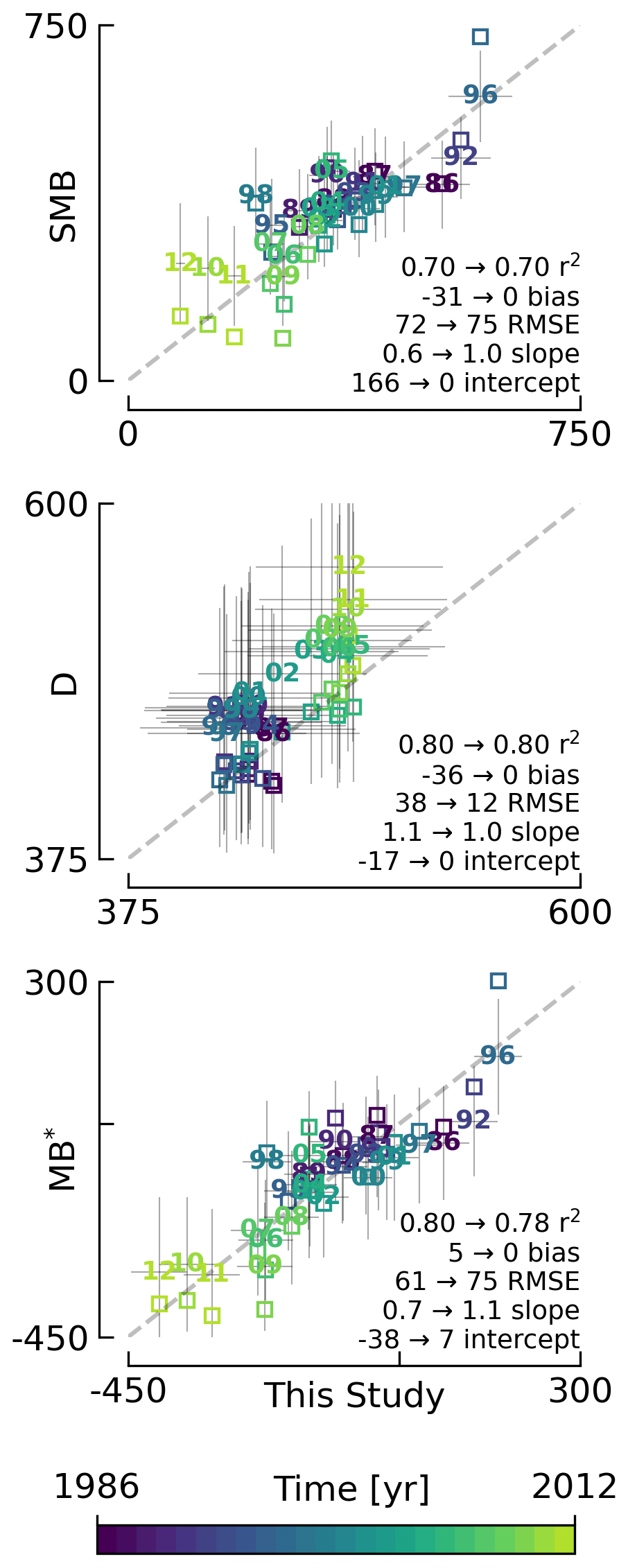
Figure 3 Comparison between This Study and the reconstruction (Kjeldsen et al., 2015). All axis units are Gt yr⁻¹. Plotted numbers represent the last two digits of the years for the unadjusted data sets. The matching colored squares show the adjusted data. MB^* shown here does not include BMB for either the reconstructed or This Study data. Arrows show statistical properties before and after the adjustment. No adjustment is made to MB^*, but it is computed from Eq. (4) both before (numbered) and after (squares) the surface and discharge adjustments.

The reconstructed surface mass balance is adjusted as described in the Methods Sect. 5.4 (Fig. 3).

4.2 Discharge

The recent discharge data are from Mankoff et al. (2020b) (data: Mankoff and Solgaard, 2020). This product covers all fast-flowing (>100 m yr⁻¹) marine-terminating glaciers. The discharge in Mankoff et al. (2020b) is computed at flux gates ∼5 km upstream from glacier termini (Mankoff, 2020) using a wide range of velocity products and ice thickness from BedMachine v4. Discharge across flux gates is derived with a 200 m spatial resolution grid but then summed and provided at glacier resolution. Temporal coverage begins in 1986 with a few velocity estimates and is updated each time a new velocity product is released, which is every ∼12 d with a ∼30 d lag (Solgaard et al., 2021; data: Solgaard and Kusk, 2021).

Some changes have been implemented since the last publication describing the discharge product (i.e., Mankoff et al., 2020b). These are minor and include updating the Khan et al. (2016) (data: Khan, 2017) surface elevation change product from 2015 through 2019, updating various MEaSUREs velocity products to their latest version, updating the PROMICE Sentinel ice velocity product from Edition 1 (https://doi.org/10.22008/promice/data/sentinel1icevelocity/greenlandicesheet/v1.0.0) to Edition 2 (Solgaard et al., 2021; Solgaard and Kusk, 2021), and updating from BedMachine v3 (supplemented in the SE with Millan et al., 2018) to use only BedMachine v4 (Morlighem et al., 2021).

The reconstructed discharge data (Kjeldsen et al., 2015) are estimated via a linear fit between unsmoothed annual discharge spanning 2000 to 2012 (Enderlin et al., 2014) and runoff data from Kjeldsen et al. (2015) using a 6-year trailing average. The method for scaling discharge from runoff was introduced by Rignot et al. (2008), who scaled the SMB anomaly with discharge. Sensitivity analyses conducted by Box and Colgan (2013) showed runoff to be the more effective discharge predictor and include a discussion of the physical basis. Although the fitting period of the present data set includes an anomalous period of discharge (2000 through 2005; e.g., Boers and Rypdal, 2021), the discharge data used by Rignot et al. (2008) and Box and Colgan (2013) also include years 1958 and 1964 that lie near the regression line (see Box and Colgan, 2013, Fig. 4, and the related Sect. 4, Physical basis). Further, while 2000 through 2005 cover a changing period in Greenlandic discharge (Mankoff et al., 2020b; King et al., 2020), there were likely other anomalous periods in the past, when glaciers in Greenland experienced considerable increases in discharge, as inferred by geological and geodetic investigations (Andresen et al., 2012; Bjørk et al., 2012; Khan et al., 2015, 2020).

The reconstructed discharge is adjusted as described in the Methods Sect. 5.4.

4.3 Basal mass balance

The BMB (Karlsson et al., 2021) comes from mass lost at the bed from BMB_GF, BMB_friction from the basal shear velocity, and BMB_VHD from surface runoff routed to the bed (i.e., the volume of the subglacial conduits formed from surface runoff; Mankoff and Tulaczyk, 2017). These fields (data: Karlsson, 2021) are provided as steady-state annual estimates. We use the BMB_GF and BMB_friction products and apply $\mathrm{1}/\mathrm{365}$th to each day, each year. Because BMB_VHD is proportional to runoff, an annual estimate is not appropriate for this work with daily resolution. We therefore re-calculate the BMB_VHD-induced basal melt as described in the Methods Sect. 5.3.

4.3.1 Geothermal flux

Due to a lack of direct observations, the geothermal flux is poorly constrained under most of the Greenland ice sheet. Different approaches have been employed to infer the value of the BMB_GF, often with diverging results (see, e.g., Rogozhina et al., 2012; Rezvanbehbahani et al., 2019). Lacking substantial validation that favors one BMB_GF map over the others, Karlsson et al. (2021) instead use the average of three widely used BMB_GF estimates: Fox Maule et al. (2009), Shapiro and Ritzwoller (2004), and Martos et al. (2018). The BMB_GF melt rate is calculated as

$$\begin{array}{}\text{(1)}& {\displaystyle }{\displaystyle }{\dot{b}}_{\mathrm{m}}=E_{\text{GF}}{\mathit{\rho }}_{\mathrm{i}}^{-\mathrm{1}}{L}^{-\mathrm{1}},\end{array}$$

where E_GF is available energy at the bed, here the geothermal flux in unit W m⁻², ρ_i is the density of ice (917 kg m⁻³), and L is the latent heat of fusion (335 kJ kg⁻¹; Cuffey and Paterson, 2010). BMB_GF melting is only calculated where the bed is not frozen. We use the MacGregor et al. (2016) estimate of temperate bed extent and scale Eq. (1) by 0, 0.5, or 1 where the bed is frozen (∼25 % of the ice sheet area), uncertain (∼33 %), or thawed (∼42 %), respectively.

4.3.2 Friction

This heat term stems from the friction produced as ice slides over the bedrock. The term has only been measured in a handful of places (e.g., Ryser et al., 2014; Maier et al., 2019), and it is unclear how representative those measurements are at ice sheet scales. Karlsson et al. (2021) therefore estimate the frictional heating using the full Stokes Elmer/Ice model that resolves all stresses while relating basal sliding and shear stress using a linear friction law (Gillet-Chaulet et al., 2012; Maier et al., 2021). The model is tuned to match a multi-decadal surface velocity map (Joughin et al., 2018) covering 1995–2015, and it returns an estimated basal friction heat that is used to calculate the basal melt due to friction, similarly to Eq. (1):

$$\begin{array}{}\text{(2)}& {\displaystyle }{\displaystyle }{\dot{b}}_{\mathrm{m}}=E_{\mathrm{f}}{\mathit{\rho }}_{\mathrm{i}}^{-\mathrm{1}}{L}^{-\mathrm{1}},\end{array}$$

where E_f is energy due to friction. We also apply the 0, 0.5, and 1 scale as used for the BMB_GF term (MacGregor et al., 2016) in order to mask out areas that are likely frozen.

4.4 Other

ROI regions come from Mouginot and Rignot (2019) and ROI sectors come from Zwally et al. (2012).

4.5 Products used for validation

We validate This Study against five other data products (see Table 2 and Sect. 6). These products are the most recent IO product (Mouginot et al., 2019), the previous PROMICE mass balance product (Colgan et al., 2019; data: Colgan, 2021), the two mostly independent methods of estimating ice sheet mass change, GMB (Barletta et al., 2013; data: Barletta et al., 2020) and VC (Simonsen et al., 2021a; data: Simonsen et al., 2021b), and the IMBIE2 data (IMBIE Team, 2019). In addition to this, we evaluate the reconstructed Kjeldsen et al. (2015) (data: Box et al., 2021) and This Study data during the overlapping period 1986 through 2012.

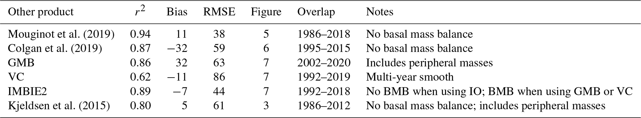
Mouginot et al. (2019)Colgan et al. (2019)Kjeldsen et al. (2015)

Table 2 Summary of correlation, bias, and RMSE between different products during their overlap periods with This Study. Basal mass balance not included in This Study when comparing against Mouginot and Rignot (2019), Colgan et al. (2019), or Kjeldsen et al. (2015). Peripheral ice masses never included in This Study.

5 Methods

The total mass balance for all of Greenland and all the different ROIs involves summing each field (SMB, D, BMB) by each ROI and then subtracting the D and BMB from the SMB fields, or

$$\begin{array}{}\text{(3)}& {\displaystyle }{\displaystyle }\text{MB}=\text{SMB}-\text{D}-\text{BMB}.\end{array}$$

Products that do not include the BMB term (i.e., Mouginot et al., 2019, Colgan et al., 2019, and Kjeldsen et al., 2015) have total mass balance defined as

$$\begin{array}{}\text{(4)}& {\displaystyle }{\displaystyle }{\text{MB}}^{*}=\text{SMB}-\text{D},\end{array}$$

and when comparing This Study to those products, we compare like terms, never comparing our MB to a different product MB^*, except in Fig. 4, where all products are shown together.

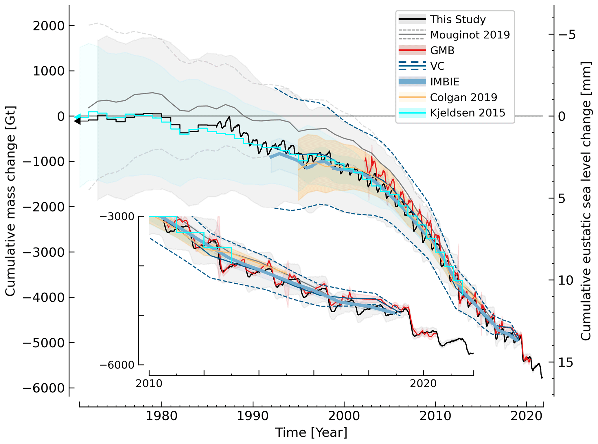
Figure 4 Comparison between This Study and other mass balance time series. Note that various products do or do not include basal mass balance or peripheral ice masses (see Table 2). This Study annual-resolution data prior to 1986 are the Kjeldsen et al. (2015) data adjusted as described in Sect. 5.4. Sea level rise calculated as $-\mathrm{Gt}/\mathrm{361.8}$. Inset highlights changes since 2010. Data product version 74 from 25 October 2021 used to generate this graphic.

Prior to calculating the mass balance, we perform the following steps.

5.1 Surface mass balance

In This Study we generate an output based on each of the three RCMs (HIRHAM/HARMONIE, MAR, and RACMO); however, in addition to these we generate a final and fourth SMB field defined as a combination of (1) the adjusted reconstructed SMB from 1840 through 1985 (Sect. 5.4) and (2) the average of HIRHAM/HARMONIE, MAR, and RACMO from 1986 through a few months ago, the average of HIRHAM/HARMONIE and MAR from a few months ago through yesterday, and MAR from yesterday through next week. See Appendix A for differences between This Study MB and MB derived using each of the RCM SMBs. There is no obvious change or step function at the 1985 to 1986 reconstructed-to-recent change nor as the RACMO and then HIRHAM/HARMONIE RCMs become unavailable a few months ago and yesterday, respectively.

5.2 Projected discharge

We project the discharge from the last observed point from Mankoff et al. (2020b) (generally between 2 weeks and 1 month old) to 7 d into the future at each glacier. We define the long-term trend as the linear least squares fit to the last 3 years of data. The residual is the data minus the long-term trend. We define the seasonal signal as the daily average from each year of the last 3 years of the residual during the temporal window of interest that spans from the most recently available observation through next week. We shift the seasonal signal so that it is 0 on the first projected day. We then assign the value of the last observation, plus the long-term trend, plus the seasonal signal to the recent past-projected and future-forecasted D.

Discharge does not change sign and changes magnitude by approximately 6 % annually over the entire ice sheet (King et al., 2018), but surface mass balance changes sign and has both larger and higher frequency variability. From this, the statistical forecast for discharge described above does not impact results as much as the physically based model forecast for surface mass balance.

5.3 Basal mass balance

Because Karlsson et al. (2021) provide a steady-state annual-average estimate of the BMB fields, we divide the BMB_GF and BMB_friction fields by 365 to estimate daily average. This is a reasonable treatment of the BMB_GF field, which does not have an annual cycle. The BMB_friction field does have a small annual cycle that matches the annual velocity cycle. However, when averaged over all of Greenland, this is only a ∼6 % variation (King et al., 2018), and Karlsson et al. (2021) found that basal melt rates are 5 % higher during the summer. Thus, the intra-annual changes are less than the uncertainty. The BMB_VHD field varies significantly throughout the year, because it is proportional to surface runoff. We therefore generate our own BMB_VHD for This Study.

To estimate recent BMB_VHD, we use daily MAR runoff (see Mankoff et al., 2020a) and BedMachine v4 (Morlighem et al., 2017, 2021) to derive subglacial routing pathways, similarly to Mankoff and Tulaczyk (2017). We assume that all runoff travels to the bed within the grid cell where it is generated, the bed is pressurized by the load of the overhead ice, and the runoff discharges on the day it is generated. We calculate subglacial routing from the gradient of the subglacial pressure head surface, h, defined as

$$\begin{array}{}\text{(5)}& {\displaystyle }{\displaystyle }h=z_{\mathrm{b}}+k{\displaystyle \frac{{\mathit{\rho }}_{\mathrm{i}}}{{\mathit{\rho }}_{\mathrm{w}}}}(z_{\mathrm{s}}-z_{\mathrm{b}}),\end{array}$$

with z_b the basal topography, k the flotation fraction (1), ρ_i the density of ice (917 kg m⁻³), ρ_w the density of water (1000 kg m⁻³), and z_s the ice surface. Equation (5) comes from Shreve (1972), where the hydropotential has units of Pascals (Pa), but here it is divided by gravitational acceleration g times the density of water ρ_w to convert the units from Pascals to meters (Pa to m).

We compute h and from h streams and outlets and both the pressure and elevation difference between the source and outlet. The energy available for basal melting is the elevation difference (gravitational potential energy) and two-thirds of the pressure difference, with the remaining one-third consumed to warm the water to match the changing phase transition temperature (Liestøl, 1956; Mankoff and Tulaczyk, 2017). We assume all energy, E_VHD (in Joules), is used to melt ice with

$$\begin{array}{}\text{(6)}& {\displaystyle }{\displaystyle }{b}_{\mathrm{m}}=E_{\text{VHD}}{\mathit{\rho }}_{\mathrm{i}}^{-\mathrm{1}}{L}^{-\mathrm{1}}.\end{array}$$

Because results are presented per ROI, and to reduce the computational load of this daily estimate, we only calculate the integrated energy released between the RCM runoff source cell and the outlet cell and then assign that to the ROI containing the runoff source cell.

To estimate reconstructed basal mass balance, we treat BMB_GF and BMB_friction as steady state as described at the start of this section. For BMB_VHD we use the fact that VHD comes from runoff by definition, and from this, reconstructed BMB_VHD is calculated using scaled runoff as a proxy. VHD theory suggests that a unit volume of runoff that experiences a 1000 m elevation drop will release enough heat to melt an additional 3 % (Liestøl, 1956). To estimate the scale factor, we use the 1986 through 2012 overlap between the Kjeldsen et al. (2015) runoff and This Study recent BMB_VHD from MAR runoff described above. The correlation between the two has an r² value of 0.75, a slope of 0.03, and an intercept of −3 Gt yr⁻¹ (Appendix D). From this, we scale the Kjeldsen et al. (2015) reconstructed runoff by 3 % (from the 0.03 slope, unrelated to the theoretical 1000 m drop described earlier) to estimate reconstructed BMB_VHD.

5.4 Reconstructed adjustment

We use the reconstructed and recent SMB and D overlap from 1986 through 2012 to adjust the reconstructed data. This Study vs. reconstructed SMB has a slope of 0.6 and an intercept of 166 Gt yr⁻¹ (Fig. 3 SMB), and This Study vs. reconstructed D has a slope of 1.1 and an intercept of −17 Gt yr⁻¹ (Fig. 3 D). The unadjusted reconstructed data slightly underestimate years with high SMB and overestimate years with low SMB (see 1986, 2010, 2011, and 2012 in Fig. 3 SMB). The unadjusted reconstructed data slightly overestimate years with low D and overestimate years with high D.

We adjust the reconstructed data until the reconstructed vs. recent slope is 1 and the intercept is 0 Gt yr⁻¹ for each of the surface mass balance and discharge comparisons (Fig. 3). We then derive the BMB_VHD term for reconstructed basal mass balance (Sect. 5.3 and Appendix D), bring in the other BMB terms (Sect. 5.3), and use Eq. (3) to compute the adjusted reconstructed mass balance.

For reconstructed SMB and D, the mean of the recent uncertainty is added to the reconstructed uncertainty during the adjustment. Reconstructed MB uncertainty is then re-calculated as the square root of the sum of the squares of the reconstructed SMB and D uncertainty.

For surface mass balance, the adjustment is effectively a rotation around the mean values, with years with low SMB decreasing and years with high SMB increasing after the adjustment. For discharge, years with low D are slightly reduced, and years with high D have a higher reduction to better match the overlapping estimates.

The adjustment described above treats all biases in the reconstructed data. The primary assumption of our adjustment is that the bias contributions do not change in proportion to each other over time. We attribute the disagreement and need for the adjustment to the demonstrated too-high biases in accumulation and ablation estimates in the 1840–2012 reconstructed SMB field (Fettweis et al., 2020), an offset resulting from differences in ice masks (Kjeldsen et al., 2015), the inclusion of peripheral glaciers (Kjeldsen et al., 2015), other accumulation rate inaccuracies (Lewis et al., 2017, 2019), and other unknowns.

5.5 Domains, boundaries, and regions of interest

Few of the ice masks used here are spatially aligned. The Zwally et al. (2012) sectors and the Mouginot and Rignot (2019) regions are often smaller than the RCM ice domains. For example, the RACMO ice domain is 1 718 959 km², of which 1 696 419 km² (99 %) are covered by the Mouginot and Rignot (2019) regions and 22 540 km² (1 %) are not, or 1 678 864 km² (98 %) are covered by Zwally et al. (2012) and 40 095 km² (2 %) are not.

Cropping the RCM domain edges would remove the edge cells where the largest SMB losses occur. This effect is minor when SMB is high (years with low runoff, assuming SMB magnitude is dominated by the runoff term). This effect is large when SMB is low (years with high runoff). As an example of the 2010 decade, RACMO SMB has a mean of 251 Gt yr⁻¹ for the decade, with a low of 45 Gt in 2019 and a high of 420 Gt in 2018. For these same extreme years RACMO cropped to Mouginot and Rignot (2019) has a low of 76 Gt (68 % high) and a high of 429 Gt (2 % high). RACMO cropped to Zwally et al. (2012) has a low of 84 Gt (85 % high) and a high of 429 Gt (2 % high).

We therefore grow the ROIs to cover the RCM domains. ROIs are grown by expanding them outward, assigning the new cells the value (ROI classification, that is, sector number or region name; see Fig. 1) of the nearest non-null cell, and then clipping to the RCM ice domain. This is done for each ROI and RCM. Appendix E provides a graphical display of the HIRHAM RCM domain, the Mouginot and Rignot (2019) domain, and our expanded Mouginot and Rignot (2019) domain.

BMB_VHD comes from the MAR ice domain runoff but is generated on the BedMachine ice thickness grid, which is smaller than the ice domain in some places. Therefore, the largest runoff volumes per unit area (from the low-elevation edge of the ice sheet) are discarded in these locations.

6 Product evaluation and assessment

We compare to six related data sets (see Table 2 and Sect. 4.5): the most similar and recent IO product (Mouginot et al., 2019), the previous PROMICE assessment (Colgan et al., 2019), the two mostly independent methods (GMB, Barletta et al., 2013, and VC, Simonsen et al., 2021a), IMBIE2 (IMBIE Team, 2019), and the unadjusted reconstructed/recent overlap (Kjeldsen et al., 2015).

Our initial comparison (Fig. 4) shows all seven products overlaid in a time series accumulating at the product resolution (daily to annual) from the beginning of the first overlap (1972, Mouginot et al., 2019) until 7 d from now (now defined as 25 October 2021 based on the date this document is compiled). Each data set is manually aligned vertically so that the last timestamps appear to overlap, allowing disagreements to grow back in time. We also assume errors are smallest at present and allow errors to grow back in time. The errors for this product are described in the Uncertainty section.

In the sections below, we compare This Study to each of the validation data in more detail. The Mouginot et al. (2019) and Colgan et al. (2019) products allow term-level (SMB, D, and MB^*) comparison and the GMB, VC, and IMBIE2 only MB-level comparison. The MB or MB^* comparison for each product is summarized in Table 2. All have different masks. Bias (Gt yr⁻¹) is defined as $\frac{\mathrm{1}}{n}{\sum }_{i=\mathrm{1}}^n(x_i-y_i)$. Root mean square error (RMSE) (Gt yr⁻¹) is defined as $\sqrt{\frac{\mathrm{1}}{n}{\sum }_{i=\mathrm{1}}^n(x_i-y_i{)}^{\mathrm{2}}}$. Sums are computed using ice-sheet-wide annual values, where x is This Study, y is the other product, and a positive bias means that This Study has a larger value.

6.1 Mouginot (2019)

The Mouginot et al. (2019) product spans the 1972 through 2018 period. We only use 1986 and onward because This Study has annual resolution prior to 1986 and Mouginot et al. (2019) data are provided on a non-calendar-year period. The SMB comes from RACMO v2.3p2 downscaled at 1 km and agrees very well with SMB from This Study (r² 0.94, bias 11, RMSE 38, slope 1.1). The minor SMB differences are likely due to mask differences or our use of a three-RCM average SMB estimate.

Mouginot et al. (2019) discharge and our D from Mankoff et al. (2020b) have a −33 Gt yr⁻¹ bias. This difference can mainly be attributed to different discharge estimates in the southeastern and central eastern sectors (Appendix: Mouginot regions). When we include BMB in This Study (diamonds in middle panel of Fig. 5 shifting values to the right), it adds ∼25 Gt yr⁻¹ to This Study.

Because MB^* is a linear combination of SMB and D terms (Eq. 4), the MB^* differences between this product and Mouginot et al. (2019) are dominated by the D term, although it is not apparent because interannual variability is dominated by SMB.

6.2 Colgan (2019)

The Colgan et al. (2019) product spans 1995 through 2015. The SMB term is broadly similar to the RCM-averaged SMB term in This Study, although Colgan et al. (2019) use only an older version of MAR (Fig. 6 top panel). The Colgan et al. (2019) SMB is spatially interpolated over the PROMICE ice sheet ice mask (Citterio and Ahlstrøm, 2013), which contains more detail on the ice sheet periphery and therefore a larger ablation area than the native coarser MAR ice mask. This Study does not interpolate the SMB field and instead works on the SMB ice domain.

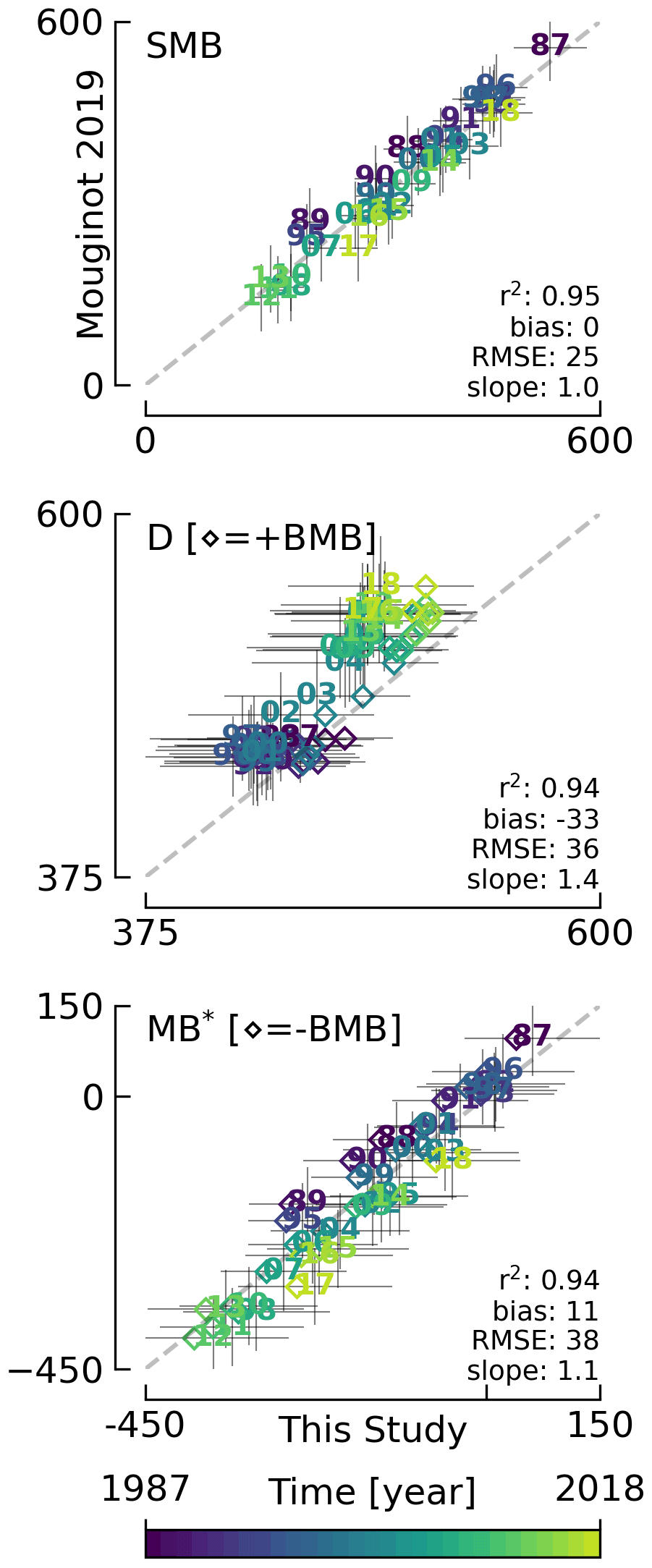
Figure 5 Comparison of This Study vs. Mouginot et al. (2019). All axis units are Gt yr⁻¹. Plotted numbers represent the last two digits of the year. Matching colored diamonds show the data when BMB is added to This Study. Printed numbers (r², bias, RMSE, slope) compare values without BMB.

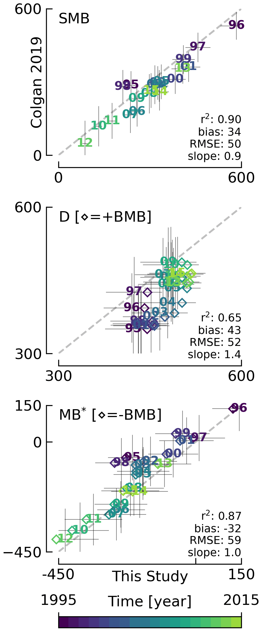
Figure 6 Comparison of This Study vs. Colgan et al. (2019). All axis units are Gt yr⁻¹. Plotted numbers represent the last two digits of the year. Matching colored diamonds show the data when BMB is added to This Study. Printed numbers (r², bias, RMSE, slope) compare values without BMB.

The largest difference between This Study and Colgan et al. (2019) is that the latter estimate grounding line ice discharge based on corrections to ice volume flow rate measured across the ∼1700 m elevation contour. This is far inland relative to the grounding line flux gates used in This Study (from Mankoff, 2020). This introduces uncertainty into the Colgan et al. (2019) D term from SMB corrections between the 1700 m elevation contour and the terminus (see the large disagreement in Fig. 6 middle panel). This disagreement increases when BMB is included in the results of This Study (shown by the annual values shifting to the right).

The D disagreement is represented differently across sectors (Appendix: Colgan 2019), where sectors 1, 2, 5, and 6 all have correlation coefficients less than ∼0.1, while the remaining sectors 3, 4, 7, and 8 all have correlation coefficients greater than 0.5.

This Study assesses greater D bias (43 Gt yr⁻¹) than Colgan et al. (2019). While Colgan et al. (2019) did not assess BMB, the majority of this discrepancy likely results from Colgan et al. (2019) aliasing the aforementioned downstream correction terms. For example, while This Study shows very little interannual variability in ice discharge in the predominantly land-terminating SW region, Colgan et al. (2019) infer large interannual variability in ice discharge based on large interannual variability in SMB and changes in ablation area ice volume in their Sector 6. The discrepancy between This Study and the Colgan et al. (2019) D[+BMB] is largest during the earliest part of the record (i.e., 1995–2000), decreasing towards the present day, which may suggest that Colgan et al. (2019) particularly overestimated the response in ice discharge to 1990s climate variability.

Similarly to the comparison with Mouginot et al. (2019), the disagreement between This Study and Colgan et al. (2019) is dominated by D disagreement, although it is again not apparent because interannual variability is dominated by SMB.

6.3 GMB

Unlike This Study, the GMB method includes mass losses and gains on peripheral ice masses which should introduce a bias of ∼10 % to 15 % (Colgan et al., 2015; Bolch et al., 2013). The inclusion of peripheral ice in the GMB product is because the spatial resolution is so low that it cannot distinguish between them and the main ice sheet. There is also signal leakage from other glaciated areas, e.g., the Canadian Arctic. This can have an effect on the estimated signal, especially in sectors 1 and 8 or regions NW and NO. There is also leakage between basins, which becomes a larger issue for smaller basins or where major outlet glaciers are near basin boundaries. GMB may also have an amplified seasonal signal due to changing snow loading in the surrounding land areas that may be mapped as ice sheet mass change variability. This would enhance the seasonal amplitude but not have an impact on the interannual mass change rates. Additionally, different glacial isostatic adjustment (GIA) corrections applied to the gravimetric signal may also lead to differences in GMB estimates on an ice sheet scale but also on a sector scale (e.g., Sutterley et al., 2014; Khan et al., 2016).

GMB and the IO method (This Study) both report changes in ice sheet mass, but they are measuring two fundamentally different things. The IO method tracks volume flow rate across the ice sheet boundaries. Typically this is meltwater across the ice sheet surface and solid ice across flux gates near the calving edge of the ice sheet, and in This Study also meltwater across the ice sheet basal boundary. That volume is then converted to mass. We consider that mass is “lost” as soon as it crosses the boundary (i.e., the ice melts or ice crosses the flux gate). The GMB method tracks the regional mass changes. Melting ice has no impact on this until the meltwater enters the ocean and a similar mass leaves the far-field GMB footprint. From these differences, the GMB method may be a better estimate of sea level rise, while the IO method may be a better representation of the state of the Greenland ice sheet.

6.4 VC

When deriving surface elevation change from satellite altimetry, data from multiple years are needed to give a stable ice-sheet-wide prediction. Hence, the altimetric mass balance estimates are often reported as averages of single satellite missions.

Although This Study has a small (−𝟷𝟷 Gt yr⁻¹) bias in comparison to Simonsen et al. (2021a) VC, there is a relatively high RMSE of 86 Gt yr⁻¹ and a mid-range correlation (r²=0.62). This suggests that while both This Study and VC agree on the total mass loss of the ice sheet, they disagree on the precise temporal distribution of this mass loss. It is possible that the outlying 1992 and 2019 years are influenced by the edge of the time series record if not fully sampled, but other outliers exist – the 1992 extreme low melt year and the 2019 extreme melt year as well as the 1995 through 1998 period stand out as years with poor agreement.

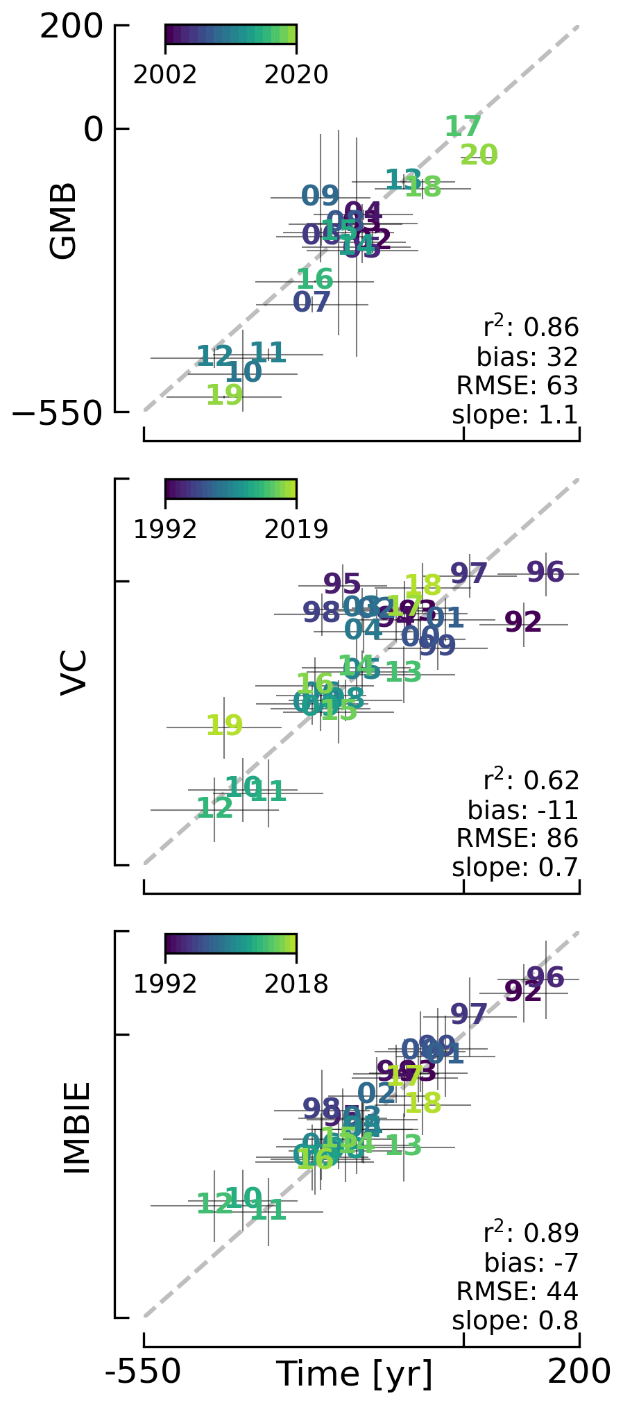
Figure 7 This Study total mass balance (MB) vs. the gravimetric method (GMB), volume change method (VC), and IMBIE2 estimates of MB. All three include BMB. All axis units are Gt yr⁻¹. Plotted numbers represent the last two digits of the year. GRACE and IMBIE2 include peripheral ice masses.

We suggest that this is due to climate influences on the effective radar horizon across the ice sheet during these years. Weather-driven change in the effective scatter horizon, mapped by the Ku band in the upper snow layer of ice sheets, hampers the conversion of radar-derived elevation change into mass change (Nilsson et al., 2015). Simonsen et al. (2021a) used a machine learning approach to derive a temporal calibration field for converting the radar elevation change estimates into mass change. This approach relied on precise mass balance estimates from ICESat to train the model and thereby was able to remove the effects of the changing scattering horizon in the radar data. This VC mass balance is given for monthly time steps (Simonsen et al., 2021a); however, the running mean applied to derive radar elevation change will dampen the interannual variability of the mass balance estimate from VC. This is especially true prior to 2010, after which the novel radar altimeter onboard CryoSat-2 allowed for a shortening of the data windowing from 5 to 3 years. This smoothing of the interannual variability is also seen in the intercomparison between This Study and the VC MB, where in addition to the two end-members of the time series (1992 and 2019) the years 1995, 1996, and 1998 seem to be outliers (Fig. 7). These years are notable for high MB, which seems to be captured less precisely by the older radar altimeters due to the longer temporal averaging.

6.5 IMBIE

The most widely cited estimate of Greenland mass balance today is the Ice-Sheet Mass Balance Inter-Comparison Exercise 2 (IMBIE2, IMBIE Team, 2019). IMBIE2 seeks to provide a consensus estimate of monthly Greenland mass balance between 1992 and 2018 that is derived from altimetry, gravimetry, and input–output ensemble members. There are two critical methodological differences between This Study and IMBIE2. Firstly, the gravimetry members of IMBIE2 assess the mass balance of all Greenlandic land ice, including peripheral ice masses, while This Study only assesses the mass balance of the ice sheet proper. Secondly, the input–output members of IMBIE2 do not assess BMB, while This Study does.

The IMBIE2 composite record of ice sheet mass balance equally weights three methods of assessing ice sheet mass balance: input–output, altimetry, and gravimetry. Prior to ca. 2003, however, IMBIE2 is derived solely from IO studies that explicitly exclude BMB (MB is actually MB^*). After ca. 2003, by comparison, IMBIE2 includes both satellite altimetry and gravimetry records implicitly sampling BMB. The representation of BMB in the composite IMBIE2 mass balance record therefore shifts before and after ca. 2003.

In comparison to mass balance assessed by IMBIE2, This Study has a small bias of ∼-7 Gt yr⁻¹ over the 26-calendar-year comparison period. This apparent agreement may be attributed to the compensating effects of IMBIE2 effectively sampling peripheral ice masses and ignoring BMB, while This Study does the opposite and ignores peripheral ice masses but samples BMB, equal to ∼25 Gt yr⁻¹. Over the entire 26-year comparison period, the RMSE with IMBIE2 is 44 Gt yr⁻¹ and the correlation is 0.89. This relatively high correlation highlights good agreement in interannual variability between studies, and the RMSE suggests that formal stated uncertainties of each study (ca. ±30 to ±63 Gt yr⁻¹ for IMBIE2 and a mean of 86 Gt yr⁻¹ for This Study) are indeed good estimates of the true uncertainty, as assessed by inter-study discrepancies.

7 Uncertainty

We treat the three inputs to the total mass balance (surface mass balance, discharge, and basal mass balance, or SMB, D, and BMB) as independent when calculating the total error. This is a simplification – the RCM SMB and the BMB_VHD from RCM runoff are related and D ice thickness and BMB_VHD pressure gradients are related, and other terms may have dependencies. However, the two dominant IO terms, SMB inputs and D outputs, are independent on annual timescales, and for simplification we treat all terms as independent. We use Eq. (3) and standard error propagation for SMB, D, and BMB terms (i.e., the square root of the sum of the squares of the SMB plus D plus BMB error terms). For D, extra work is done to calculate uncertainty between the last Mankoff et al. (2020b) D data (up to 30 d old, with an error of ∼9 % or ∼45 Gt yr⁻¹) and the forecasted now-plus-7 d D (see Sect. 7.1). Table 3 provides a summary of the uncertainty for each input.

Langen et al. (2017)Fettweis et al. (2020)Noël et al. (2019)Kjeldsen et al. (2015)Mankoff et al. (2020b)(Mankoff, 2021)Kjeldsen et al. (2015)Karlsson et al. (2021)Karlsson et al. (2021)

Table 3 Summary of uncertainty estimates for products used in This Study. This is an approximate and simplified representation – RCM uncertainties are calculated separately for gain and loss terms, because SMB near 0 does not mean uncertainty is near 0. This is also why the final This Study uncertainty is presented with units Gt yr⁻¹.

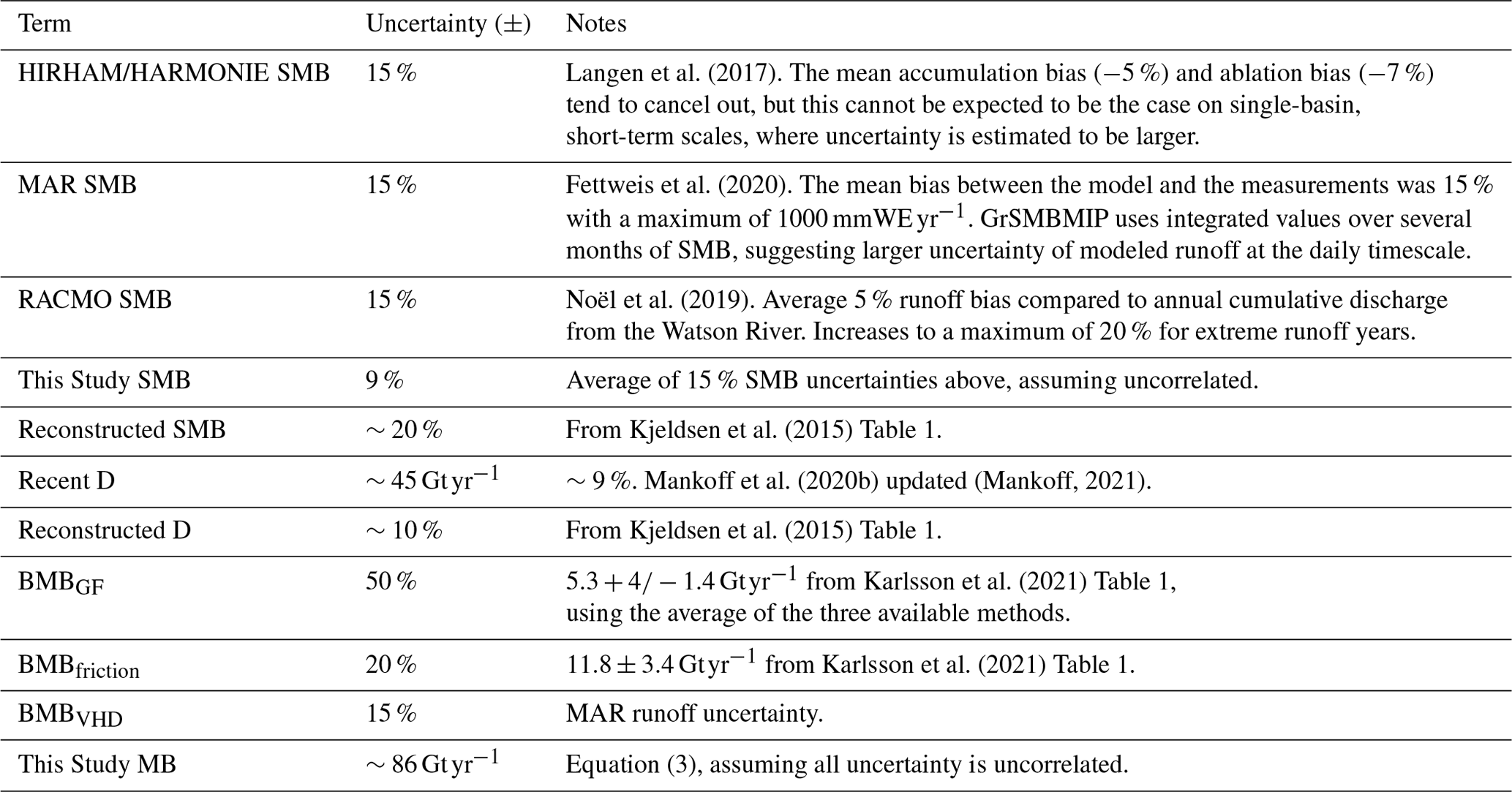
The final This Study MB uncertainty value shown in Table 3 comes from the mean of the annual sum of the MB error term.

7.1 Discharge

The D uncertainty is discussed in detail in Mankoff et al. (2020b), but the main uncertainties come from unknown ice thickness, the assumption of no vertical shear at fast-flowing marine-terminating outlet glaciers, and ice density of 917 kg m⁻³. Regional ice density can be significantly reduced by crevasses. For example, Mankoff et al. (2020c) identified a snow-covered crevasse field with 20 % crevasse density, meaning at that location regional firn density should be reduced by 20 %.

Temporally, D at daily resolution comes from ∼12 d observations upsampled to daily, and those ∼12 d resolution observations come from longer time period observations (Solgaard et al., 2021). Because the velocity method uses feature tracking, it is correct on average but misses variability within each sample period (e.g., Greene et al., 2020).

Spatially, discharge is estimated ∼5 km upstream from the grounding lines for ice velocities as low as 100 m yr⁻¹. That ice accelerates toward the margin, but even ice flowing steadily at 1 km yr⁻¹ would take 5 years before that mass is lost. However, at any given point in time, ice that had previously crossed the flux gate is calving or melting into the fjord. The discrepancy here between the flux gate estimated mass loss and the actual mass lost at the downstream terminus is only significant for glaciers that have had large velocity changes at some point in the recent past, large changes in ice thickness, or large changes in the location (retreat or advance) of the terminus. We do not consider SMB changes downstream of the flux gate, because the gates are temporally near the terminus for most of the ice that is fast-flowing, and the largest SMB uncertainty is at the ice sheet margin, where there are both mask issues and high topographic variability.

The forecasted D uncertainty is the average historical uncertainty plus a 1 % increase per day for the past projected and forecasted period.

7.2 ROIs

We work on the three different domains of the three RCMs and expand the ROIs to match the RCMs (see Appendix E). However, some alignment issues cannot be solved. For example, we use BedMachine ice thickness to estimate BMB_VHD. Often, the largest BMB_VHD occurs near the ice margin under ice with the steepest surface slopes. This is also where the largest runoff often occurs, because the ice margin, at the lowest elevations, is exposed to the warmest air. If these RCM ice grid cells with high runoff are anywhere inside the BedMachine ice domain, that runoff is still included in our BMB_VHD estimates because it flows outward and passes through the BedMachine near-ice-edge grid cells with the large pressure gradients. However, any RCM ice runoff outside the BedMachine ice domain (ice thickness is 0) is ignored.

The MAR ice domain is 1 825 600 km², of which 1 708 400 km² (94 %) are covered by the BedMachine ice mask and 26 400 km² (6 %) are not. This 6 % area contributes ∼18 % of runoff on average (range of 16 % to 21 % from 2010 through 2019). This 18 % of runoff is excluded from the VHD calculations and likely contributes more than 18 % to the VHD term, because the border region of the ice sheet has the steepest gradients and the largest volume of subglacial flow.

We encourage RCM developers, BedMachine, and others to use a common and up-to-date mask (see Kjeldsen et al., 2020).

7.3 Accumulating uncertainties

When accumulating errors as in Fig. 4, we use only the D and BMB_GF uncertainty. The D uncertainty is primarily due to unknown ice thickness and is invariant in time, and the geothermal heat flux is steady state. SMB uncertainty is assumed to have errors randomly distributed in time (for the purposes of Fig. 4). There may be time-invariant biases in the BMB_friction and SMB fields, but treating all uncertainties as biases is incorrect – evidence for that comes from the six other MB estimates. This distinction between bias and random uncertainty is only done for Fig. 4, where errors accumulate in time. The provided data product contains one uncertainty field and does not distinguish between systematic and random uncertainty. We caution others in treating SMB uncertainty as random in time for analyses that go beyond the graphical display used here.

The shaded region in Fig. 4 representing the uncertainty for This Study is computed as 365 d rolling smoothly from 1840 through 1999 of the above-described uncertainty, 1/365th of the annual error at now +7 d, and a linear blend, from 2000 to now +7 d, between the smoothed reconstructed uncertainty and the present and future more variable uncertainty.

The Mouginot et al. (2019), Colgan et al. (2019), and Kjeldsen et al. (2015) products all provide an error estimate but do not distinguish between temporally fixed errors (biases; should accumulate in time) vs. temporally random errors.

We treat the Mouginot et al. (2019) data the same as This Study. Discharge uncertainty is treated as a bias and accumulates, and surface mass balance uncertainty is treated as random and does not accumulate.

The Colgan et al. (2019) vs. This Study bias and RMSE are −32 and 59 Gt yr⁻¹, respectively. This suggests that in any given year, there could be up to $-\mathrm{32}\pm \mathrm{59}$ or $+\mathrm{27}/-\mathrm{91}$ Gt yr⁻¹ departure from This Study. From this, we assign a 32 Gt yr⁻¹ bias (35 %; accumulates in time) and a 59 Gt yr⁻¹ RMSE (65 %; random in time).

The adjusted Kjeldsen et al. (2015) data have 0 surface mass balance and discharge bias by definition (Sect. 5.4), but Fig. 4 displays the unadjusted data, and we apply a 36 Gt yr⁻¹ accumulating uncertainty from the unadjusted D bias (Fig. 3).

7.4 Peripheral ice masses

Greenland's peripheral glaciers and ice caps are not included in this product. Nonetheless, we briefly summarize recent mass balance estimates of these areas. Greenlandic peripheral ice contributes more runoff per unit area than the main ice sheet – it is <5 % of the total ice area but contributes ∼15 % to 20 % of the whole island mass loss (Bolch et al., 2013). From 2003 to 2009 and using the VC method (altimetry), Gardner et al. (2013) estimate $-\mathrm{38}\pm \mathrm{7}$ Gt yr⁻¹ peripheral mass balance. From 2006 to 2016 and using the VC method (DEM differencing), Zemp et al. (2020) estimate $-\mathrm{51}\pm \mathrm{17}$ Gt yr⁻¹ peripheral mass balance using Rastner et al. (2012) delineations.

8 Results

From the 181 complete years of data (excluding partial 2021), the mean mass balance is $-\mathrm{77}\pm \mathrm{125}$ Gt yr⁻¹, with a minimum of $-\mathrm{428}\pm \mathrm{110}$ Gt in 2012 (SMB of 87±8 Gt, D of 485±46 Gt, BMB of 29±6 Gt) and a maximum of 142±83 Gt yr⁻¹ in 1996 (SMB of 584±53 Gt, D of 420±39 Gt, BMB of 21±5 Gt).

At the decadal average, the following trends are apparent. Surface mass balance has decreased from a high of ∼450 Gt yr⁻¹ in the 1860s to a low of ∼260 Gt yr⁻¹ in the 2010s. SMB variability has also increased during this time. Discharge has increased slightly from a low of ∼375 Gt yr⁻¹ in the 1860s to a high of ∼490 Gt yr⁻¹ in the 2010s. Basal mass balance, from runoff as a proxy, had a high of 26±16 Gt yr⁻¹ in the 1930s and a low of 22±5 Gt yr⁻¹ in the 1990s but, as with runoff, has been increasing in recent decades.

The total mass balance decadal trend from the 1840s through the 2010s is one of general mass decrease and increased intra-decadal variability. The record begins in the 1840s with $\sim -\mathrm{10}$ Gt yr⁻¹, has only 1 (of 19) decades with a mass gain (∼50 Gt yr⁻¹ in the 1860s), and has a record low of $\sim -\mathrm{250}$ Gt yr⁻¹ in the 2010s.

9 Data availability

The RCM surface mass balance and the VHD basal mass balance components are updated daily, the discharge approximately every 12 d, and all are used to produce the final daily-updating product. The data area is available at https://doi.org/10.22008/FK2/OHI23Z (Mankoff et al., 2021), with all historical (daily updated) versions archived.

As part of our commitment to making continual and improving updates to the data product, we introduce a GitHub database (https://github.com/GEUS-Glaciology-and-Climate/mass_balance/, last access: 26 October 2021, Mankoff, 2021) where users can track progress, make suggestions, and discuss, report, and respond to issues that arise during use of this product.

10 Conclusions

This study is the first to provide a data set containing more than a century and real-time estimates detailing the state of Greenland ice sheet mass balance, with regional or sector spatial and daily temporal resolution products of surface mass balance, discharge, basal mass balance, and the total mass balance.

IMBIE2 highlights that during the GRACE satellite gravimetry era (2003 through 2017), there are usually more than 20 independent estimates of annual Greenland ice sheet mass balance. Just two independent estimates, however, are available prior to 2003. This study will therefore provide additional insight into ice sheet mass balance during the late 1980s and 1990s. IMBIE2 also highlights how the availability of mass balance estimates declines in the year prior to IMBIE2 publication. This reflects a lag period during which mass balance assessments from non-operational products are undergoing peer review. The operational nature of this product supports the timely inclusion of annual MB estimates in community consensus reports such as those from IMBIE and the IPCC.

As such, the data products provided in This Study present the first operational monitoring of the Greenland ice sheet total mass balance and its components. One property of the input–output approach used in This Study is the explanatory capabilities of the data products, allowing scrutiny of the physical origins of recorded mass changes. By excluding peripheral ice masses, This Study allows and invites anyone to keep an eye on the current evolution of the Greenland ice sheet proper. However, as the spatial resolutions of RCMs increase and estimates of peripheral ice thickness become available, our setup allows inclusion of these ice masses to generate a full Greenland-wide product. Moreover, as the determination of each of the individual components of the ice sheet mass balance is expected to improve over time through international research efforts, the total mass balance product presented will also be able to improve, as it is sustained by the Danish–Greenlandic governmental long-term monitoring effort – PROMICE.

Appendix A: RCM differences

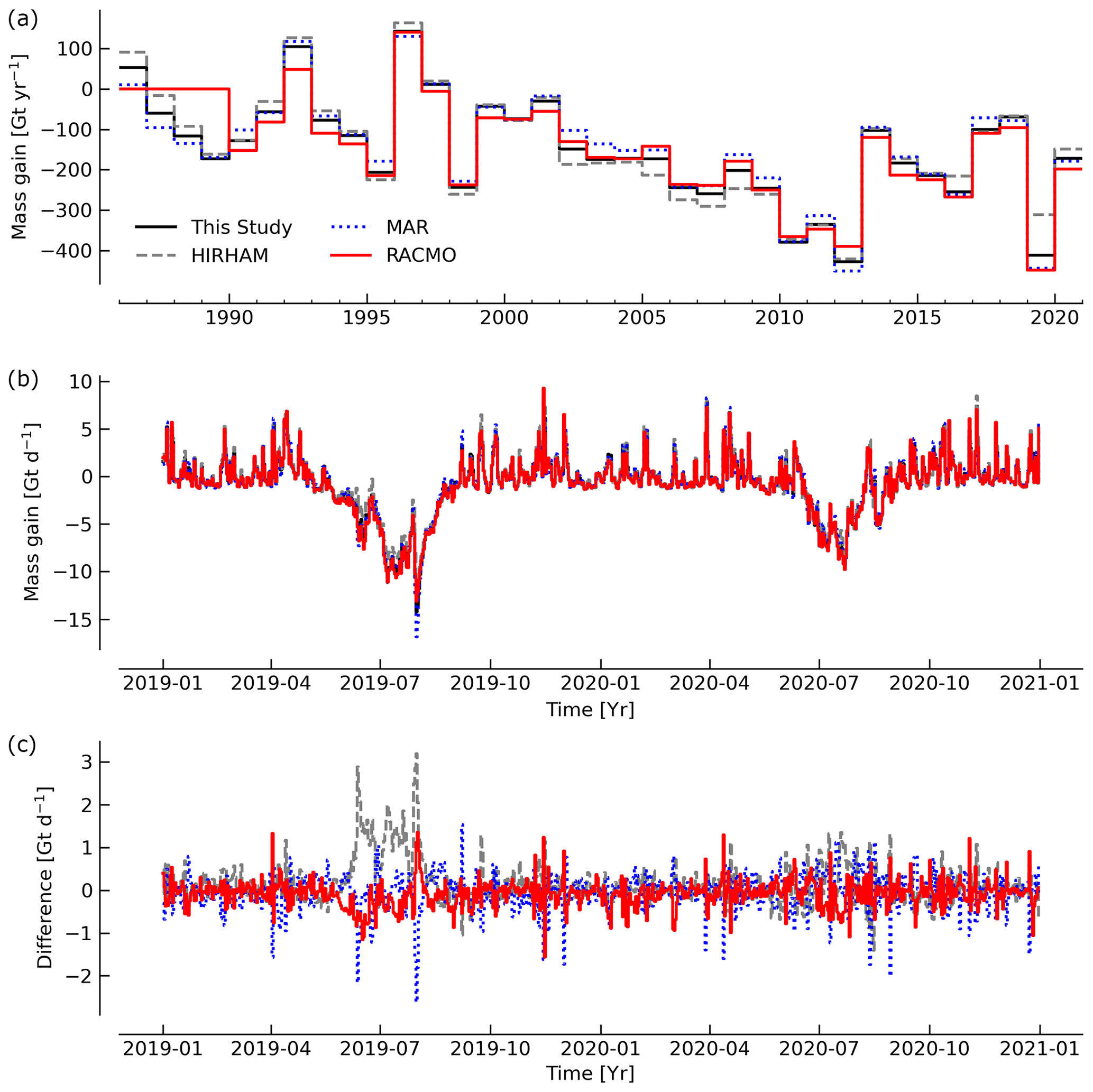
Figure A1 Comparison of This Study combined RCM product and the HIRHAM/HARMONIE, MAR, and RACMO RCMs. Results shown here are MB, not SMB, but the same D and BMB have been subtracted from each SMB product. (a) Annual MB for the entire time series. (b) Example 2 years (2019 and 2020) at daily resolution. (c) Difference between the three RCM MB products and This Study RCM-averaged product for the same data shown in panel (b).

Appendix B: Mouginot 2019 by region

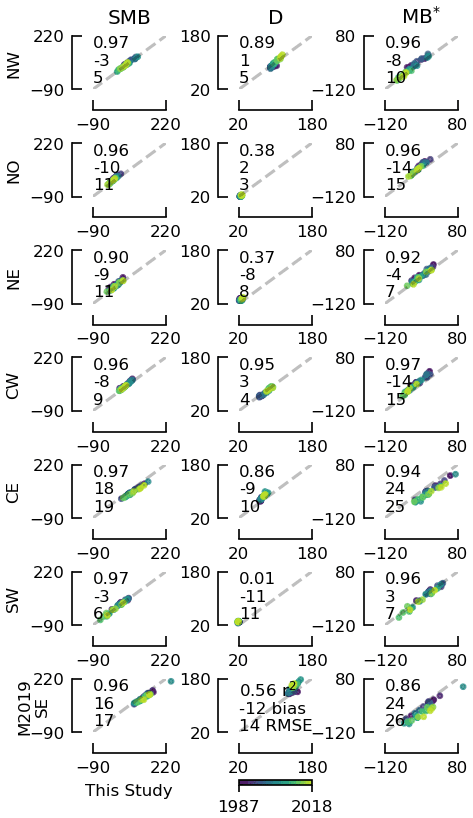
Figure B1 Comparison between This Study (excluding BMB) and Mouginot et al. (2019). Same data and display as Fig. 5 except here displayed by the Mouginot and Rignot (2019) region. Numbers in each graph show r², bias, and RMSE from top to bottom, respectively. All axis units are Gt yr⁻¹.

Appendix C: Colgan 2019 by sector

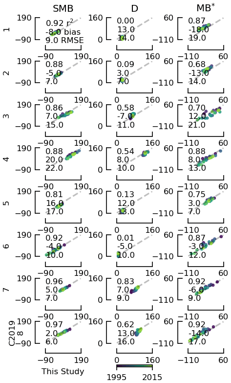
Figure C1 Comparison between This Study (excluding BMB) and Colgan et al. (2019). Same data and display as Fig. 6 except here displayed by the Zwally et al. (2012) sector. Numbers in each graph show r², bias, and RMSE from top to bottom, respectively. All axis units are Gt yr⁻¹.

Appendix D: Reconstructed runoff

Figure D1 Comparison between MAR runoff and basal viscous heat dissipation derived from that runoff. The slope is used to estimate the reconstructed BMB_VHD from reconstructed runoff (see Sect. 5.3). Axis units are Gt yr⁻¹. Plotted numbers represent the last two digits of the year.

Appendix E: RCM coverage

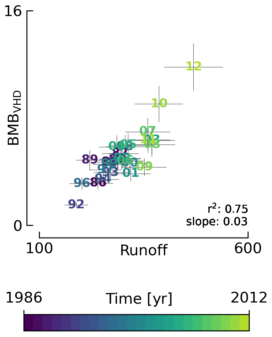
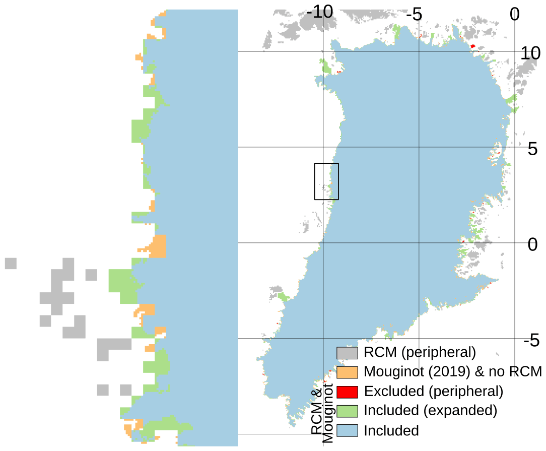
Figure E1 HIRHAM RCM coverage by Mouginot and Rignot (2019). Coverage of HIRHAM by Zwally et al. (2012), and MAR and RACMO by Mouginot and Rignot (2019) and Zwally et al. (2012) are similar to the graphic shown here (see Sect. 5.5 for a discussion of RACMO coverage issues). HIRHAM latitude and longitude cover the Equator because we work on the native HIRHAM rotated pole coordinate system.

Appendix F: Software

This work was performed using only open-source software, primarily GRASS GIS (Neteler et al., 2012), CDO (Schulzweida, 2019), NCO (Zender, 2008), GDAL (GDAL/OGR contributors, 2020), and Python (Van Rossum and Drake Jr, 1995), in particular the Jupyter (Kluyver et al., 2016), dask (Dask Development Team, 2016; Rocklin, 2015), pandas (McKinney, 2010), numpy (Oliphant, 2006), x-array (Hoyer and Hamman, 2017), and Matplotlib (Hunter, 2007) packages. The entire work was performed in Emacs (Stallman, 1981) using Org Mode (Schulte et al., 2012) on GNU/Linux and using many GNU utilities. The parallel (Tange, 2011) tool was used to speed up processing.

Appendix G: CRediT

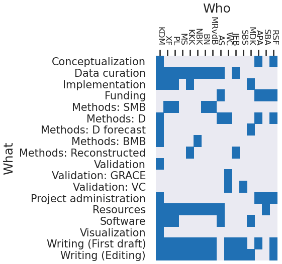
Figure G1 Author contributions following the CRediT system (Allen et al., 2014; Brand et al., 2015; Allen et al., 2019).