the Creative Commons Attribution 4.0 License.
the Creative Commons Attribution 4.0 License.
 | 23 Sep 2021
The cooperative IGS RT-GIMs: a reliable estimation of the global ionospheric electron content distribution in real time
Manuel Hernández-Pajares
Heng Yang
Enric Monte-Moreno
David Roma-Dollase
Alberto García-Rigo
Zishen Li
Ningbo Wang
Denis Laurichesse
Alexis Blot
Qile Zhao
Qiang Zhang
André Hauschild
Loukis Agrotis
Martin Schmitz
Gerhard Wübbena
Andrea Stürze
Andrzej Krankowski
Stefan Schaer
Joachim Feltens
Attila Komjathy
Reza Ghoddousi-Fard
The Real-Time Working Group (RTWG) of the International GNSS Service (IGS) is dedicated to providing high-quality data and high-accuracy products for Global Navigation Satellite System (GNSS) positioning, navigation, timing and Earth observations. As one part of real-time products, the IGS combined Real-Time Global Ionosphere Map (RT-GIM) has been generated by the real-time weighting of the RT-GIMs from IGS real-time ionosphere centers including the Chinese Academy of Sciences (CAS), Centre National d'Etudes Spatiales (CNES), Universitat Politècnica de Catalunya (UPC) and Wuhan University (WHU). The performance of global vertical total electron content (VTEC) representation in all of the RT-GIMs has been assessed by VTEC from Jason-3 altimeter for 3 months over oceans and dSTEC-GPS technique with 2 d observations over continental regions. According to the Jason-3 VTEC and dSTEC-GPS assessment, the real-time weighting technique is sensitive to the accuracy of RT-GIMs. Compared with the performance of post-processed rapid global ionosphere maps (GIMs) and IGS combined final GIM (igsg) during the testing period, the accuracy of UPC RT-GIM (after the improvement of the interpolation technique) and IGS combined RT-GIM (IRTG) is equivalent to the rapid GIMs and reaches around 2.7 and 3.0 TECU (TEC unit, 1016 el m−2) over oceans and continental regions, respectively. The accuracy of CAS RT-GIM and CNES RT-GIM is slightly worse than the rapid GIMs, while WHU RT-GIM requires a further upgrade to obtain similar performance. In addition, a strong response to the recent geomagnetic storms has been found in the global electron content (GEC) of IGS RT-GIMs (especially UPC RT-GIM and IGS combined RT-GIM). The IGS RT-GIMs turn out to be reliable sources of real-time global VTEC information and have great potential for real-time applications including range error correction for transionospheric radio signals, the monitoring of space weather, and detection of natural hazards on a global scale. All the IGS combined RT-GIMs generated and analyzed during the testing period are available at https://doi.org/10.5281/zenodo.5042622 (Liu et al., 2021b).
- Article
(1466 KB) - Full-text XML
- BibTeX
- EndNote


The global ionosphere maps (GIMs), containing vertical total electron content (VTEC) information at given grid points (typically with a spatial resolution of 2.5∘ in latitude and 5∘ in longitude), have been widely used in both scientific and technological communities (Hernández-Pajares et al., 2009). Due to the high quality and global distribution of VTEC estimation, GIM has been applied to investigating the behavior of the ionosphere, such as the climatology of mean total electron content (TEC), potential ionospheric anomalies before earthquakes, semiannual variations in TEC in the ionosphere, the VTEC structure of the polar ionosphere under different cases and W index for ionospheric disturbance warning (e.g., Liu et al., 2009, 2006; Zhao et al., 2007; Jiang et al., 2019; Hernández-Pajares et al., 2020; Gulyaeva and Stanislawska, 2008; Gulyaeva et al., 2013). In addition, the high accuracy of GIM enables precise range corrections for transionospheric radio signals including radar altimetry, radio telescopes and Global Navigation Satellite System (GNSS) positioning (e.g., Komjathy and Born, 1999; Fernandes et al., 2014; Sotomayor-Beltran et al., 2013; Le and Tiberius, 2007; Zhang et al., 2013a; Lou et al., 2016; Chen et al., 2020). The Center for Orbit Determination in Europe (CODE), European Space Agency (ESA), Jet Propulsion Laboratory (JPL), Canadian Geodetic Survey of Natural Resources Canada (NRCan) and Universitat Politècnica de Catalunya (UPC) agreed on the computation of individual GIMs in IONosphere map EXchange (IONEX) format and created the Ionosphere Working Group (Iono-WG) of the International GNSS Service (IGS) in 1998 (Schaer et al., 1996, 1998; Feltens and Schaer, 1998; Feltens, 2007; Mannucci et al., 1998; Hernández-Pajares et al., 1998, 1999). In the IGS 2015 workshop, the Chinese Academy of Sciences (CAS) and Wuhan University (WHU) became new Ionospheric Associate Analysis Centers (IAACs) (Li et al., 2015; Ghoddousi-Fard, 2014; Zhang et al., 2013b). Currently, there are three types of post-processed IGS GIMs at different latencies: final, rapid and predicted GIMs. With the contribution from different IAACs, the final and rapid GIMs are assessed and combined by corresponding weights and uploaded to File Transfer Protocol (FTP) or Hypertext Transfer Protocol (HTTP) servers with the latency of 1–2 weeks and 1–2 d, respectively. The 1 and 2 d predicted GIMs can provide valuable VTEC information in advance for ionospheric activities and corrections. However, the accuracy of predicted GIMs is limited due to the nonlinear variation in ionosphere and the lack of real-time ionospheric observations (Hernández-Pajares et al., 2009; García-Rigo et al., 2011; Li et al., 2018).
In order to satisfy the growing demand for real-time GNSS positioning and applications, the Real-Time Working Group (RTWG) of IGS was established in 2001 and officially started to provide real-time service (RTS) in 2013 (Caissy et al., 2012; Elsobeiey and Al-Harbi, 2016). Aside from multi-GNSS real-time data streams, the IGS-RTS also generates RT-GNSS product streams, including satellite orbits, clocks, code/phase biases and GIM. These high-quality IGS-RTS products enable precise GNSS positioning, navigation, timing (PNT), ionosphere monitoring and hazard detection. In the Radio Technical Commission for Maritime Services (RTCM) Special Committee (SC-104), the State Space Representation (SSR) correction data format is defined as the standard message (RTCM-SSR) for real-time GNSS applications. In support of flexible multi-GNSS applications within current multi-constellation and multi-frequency environments, a new format (IGS-SSR) is developed. The dissemination of IGS Real-Time Global Ionosphere Maps (RT-GIMs) adopts spherical harmonic expansion to save the bandwidth in both RTCM-SSR and IGS-SSR formats (RTCM-SC, 2014; IGS, 2020).
The accuracy of RT-GIMs is typically worse than post-processed GIMs due to the short span of ionospheric observations, sparse distribution of stations, higher noises in carrier-to-code leveling, or difficulty in carrier ambiguity estimation in real-time processing mode. While RT-GIMs perform slightly worse than post-processed GIMs, it is found that RT-GIMs are helpful to reduce the convergence time of dual-frequency precise point positioning (PPP), and they strengthen the solution (Li et al., 2013). With the corrections of RT-GIMs, the accuracy of single-frequency PPP reaches decimeter and meter level in horizontal and vertical directions (Ren et al., 2019), while the instantaneous (single-epoch) real-time kinematic (RTK) positioning over medium and long baselines is able to obtain a higher success rate of the ambiguity fixing and reliability for rover stations at a level of a few centimeters (Tomaszewski et al., 2020). In addition, the feasibility of ionospheric storm monitoring based on RT-GIMs is tested (García Rigo et al., 2017). A first fusion of IGS-GIMs and ionosonde data from the Global Ionosphere Radio Observatory (GIRO) paves the way for the improvement of real-time International Reference Ionosphere (Froń et al., 2020). Currently, the routine RT-GIMs are available from CAS, Centre National d'Etudes Spatiales (CNES), German Aerospace Center in Neustrelitz (DLR-NZ), JPL, UPC, WHU and IONOLAB (Li et al., 2020; Laurichesse and Blot, 2015; Jakowski et al., 2011; Hoque et al., 2019; Komjathy et al., 2012; Roma Dollase et al., 2015; Sezen et al., 2013). Individual RT-GIMs from different IGS centers can be gathered from IGS-RTS by means of Network Transportation of RTCM by Internet Protocol (NTRIP) (Weber et al., 2007). With the contribution of IGS RT-GIMs from CAS, CNES and UPC, a first IGS real-time combination of GIMs was generated in 2018 (Roma-Dollase et al., 2018a).
Recently, one of the IGS RT-GIMs (UPC-IonSAT) has completely changed the real-time interpolation strategy, with a significant improvement. In addition, the number of contributing centers has been increased from three to four, thanks to the participation of Wuhan University. A new version of IGS combined RT-GIM (IRTG) has been developed to improve the performance and also adapt to the newly updated IGS-SSR format. In addition, the developed software has been further parallelized to decrease the latency of IRTG computation to a few minutes (Tange, 2011). This paper summarizes the computation methods of IGS RT-GIMs from different ionosphere centers and the generation of IRTG. In addition, the performance of different RT-GIMs and the real-time weighting technique is shown and discussed. The conclusions and future improvements are given in the final section.
2.1 Real-time GNSS data processing
In order to generate RT-GIMs, the real-time GNSS observations from worldwide stations are received and transformed into slant TEC (STEC). It should be noted that extraction of STEC in an unbiased way can be obtained by fitting an ionospheric model to the observations. With the global distributed STEC, different strategies are chosen for the computation of RT-GIMs.
Currently, two methods are commonly used for the calculation of real-time STEC. The first method is the so-called carrier-to-code leveling (CCL) as shown in Eq. (3) (Ciraolo et al., 2007; Zhang et al., 2019). The geometry-free (GF) combination of pseudorange and carrier phase observations is formed to extract STEC and differential code bias (DCB) in an unbiased way by fitting an ionospheric model (for example, spherical harmonic model). Due to the typically shorter phase-arc length in real-time mode, the impact of multipath and thermal noise is higher than in post-processing mode (Li et al., 2020).
Here P1,t and P2,t are the pseudorange observations of epoch t at first and second frequencies, respectively. αGF can be approximated as . f1 and f2 are the first and second frequencies of observation. STECt is the STEC of epoch t. r is receiver and s is satellite. c is the speed of light in vacuum. Dr and Ds are the receiver differential code biases (DCBs) and satellite DCB. ϵM and ϵT are the code multipath error and thermal noise error. L1,t and L2,t are the carrier phase observations including the priori corrections (such as wind-up term) of epoch t at first and second frequencies. BGF equals B1−B2, while B1 and B2 are the carrier phase ambiguities including the corresponding phase bias at first and second frequencies, respectively. k is the length of smoothing arc from beginning epoch to epoch t, and represents the smoothed PGF of epoch t, which is significantly affected by the pseudorange multipath in real-time mode than in post-processing.

The second method is the GF combination of phase-only observations, and the BGF is estimated together with the real-time TEC model (for example, described in terms of tomographic voxel-based basis functions) in Eq. (2) (Hernández-Pajares et al., 1997, 1999). Although the STEC from the second method is accurate and free of code multipath and thermal noise in post-processing, the convergence time can affect the accuracy of the STEC, most likely in the isolated receivers. In addition, the computation methods of RT-GIMs from different IGS real-time ionosphere centers were compared in detail at the next subsection and summarized in Table 1. Some ionosphere centers (CAS, CNES, WHU) directly estimate and disseminate spherical harmonic coefficients in a sun-fixed reference frame as Eq. (4) (RTCM-SC, 2014; Li et al., 2020), while UPC generates the RT-GIM in IONEX format and transforms RT-GIM into spherical harmonic coefficients for the dissemination.
Here z is the satellite zenith angle, and Mz is the mapping function between STECt and VTECt. Hion is the height of the ionospheric single-layer assumption, and RE is the radius of the earth. VTECt is the VTEC of epoch t. NSH is the max degree of spherical harmonic expansion, and MSH is the max order of spherical harmonic expansion. n and m are corresponding indices. Pn,m is the normalized associated Legendre functions. Cn,m and Sn,m are sine and cosine spherical harmonic coefficients. φI and λI are the geocentric latitude and longitude of ionospheric pierce point (IPP). λS,t is the mean sun fixed and phase-shifted longitude of IPP of epoch t (typically shifted by 2 h to approximate TEC maximum at 14:00 LT). t is the current epoch. t0 is a common reference of shifted hours, taken as 0 h in the present broadcasting of RT-GIM for WHU and 2 h for CAS, CNES and UPC.
2.2 The computation of RT-GIMs by different IGS real-time ionosphere centers
The strategies for generating RT-GIMs differ between IGS real-time ionospheric analysis centers (ACs). In this subsection, a brief introduction on the generation of RT-GIMs from individual ACs and the strategy comparison between different ACs are given.
2.2.1 Chinese Academy of Sciences
The post-processed GIM of CAS has been computed and uploaded to IGS since 2015 (Li et al., 2015). A predicting-plus-modeling approach is used by CAS for the computation of RT-GIM (Li et al., 2020). CAS RT-GIM is generated with multi-GNSS, GPS and GLONASS L1 + L2, BeiDou B1 + B2, and Galileo E1 + E5a real-time data streams, provided by the IGS and regional GNSS tracking network stations. The real-time DCBs are estimated as part of the local ionospheric VTEC modeling using a generalized trigonometric series (GTS) function as Eq. (5). Then 3 d aligned biases are incorporated to increase the robustness of real-time DCBs (Wang et al., 2020).
Here r is receiver and s is satellite. φd and λd are the difference between IPP and station in latitude and longitude, respectively. i,j and l represent the degrees in the polynomial model and Fourier series expansion. and Sl are unknown parameters.
The real-time STEC is computed by subtracting estimated DCB in Eq. (5) from in Eq. (3), and then the STEC is converted into VTEC by means of a mapping function. The real-time VTEC from 130 global stations is directly modeled in a solar-geographic reference frame as Eq. (4). To mitigate the impacts of the unstable real-time data streams, e.g., the sudden interruption of the data streams, CAS-predicted TEC information is also included for RT-GIM computation. The broadcasted CAS RT-GIM is computed by the weighted combination of real-time VTEC spherical harmonic coefficients and predicted ionospheric information (Li et al., 2020).
2.2.2 Centre National d'Etudes Spatiales
In the framework of the RTS of the IGS, CNES has computed global VTEC in real time thanks to the CNES PPP-WIZARD project since 2014. The real-time VTEC is extracted by pseudorange and carrier phase GF combination as Eq. (3) with the help of a mapping function. The single-layer assumption in the mapping function adopts an altitude of 450 km above the Earth.
CNES also uses a spherical harmonic model for global VTEC representation, and the equation is the same as Eq. (4). Spherical harmonic coefficients are computed by means of a Kalman filter and simultaneous STEC from 100 stations of the real-time IGS network. CNES started to broadcast RT-GIM at the end of 2014 and changed spherical harmonic degrees from 6 to 12 in May of 2017 (Laurichesse and Blot, 2015).
2.2.3 Universitat Politècnica de Catalunya
UPC has been providing daily GIMs in IONEX format to IGS since 1998 (Hernández-Pajares et al., 1998, 1999; Orús et al., 2005). In order to meet the demand of real-time GIM, the second author of this paper (from UPC-IonSAT) developed the Real-Time TOMographic IONosphere model software (RT-TOMION) and started to generate the UPC RT-GIM on 6 February 2011. The phase-only GF combination as Eq. (2) is used for obtaining real-time STEC from around 260 stations, and a 4-D voxel-based tomographic ionosphere model is adopted for global electron content modeling. The ionosphere is divided into two layers in the tomographic model, and the electron density of each voxel is estimated together with the ambiguity term BGF by means of a Kalman filter in the sun-fixed reference frame. The estimated electron density is condensed at a fixed effective height (450 km) for the generation of a single-layer VTEC map, and then the VTEC interpolation method is adopted in a sun-fixed geomagnetic reference frame for filling the data gap on a global scale.
From 2011 to 2019, the kriging technique is selected by UPC for real-time VTEC interpolation. And the spherical harmonic model has been adopted by UPC since 8 September 2019. Recently, a new interpolation technique, denoted atomic decomposition interpolator of GIMs (ADIGIM), was developed. Since the global ionospheric electron content mainly depends on the diurnal, seasonal and solar variation, ADIGIM is computed by the weighted combination of good-quality historical GIMs (e.g., UQRG) with similar ionosphere conditions. The database of historical GIMs covers the last two solar cycles since 1998. The method for obtaining the weights of the linear combination of past maps is based on Eq. (6), which was first introduced in the problem of face recognition (Wright et al., 2008, 2010). While the face recognition is affected by the occlusions (such as glasses) in the face image, the reconstruction of GIM has problems in the regions that are not covered by GNSS stations. The problems have to be taken into account when selecting the past maps for combination and should not introduce a bias. As shown in Eq. (6), the problem is solved by introducing ℓ2 norm and ℓ1 norm. The property of the atomic decomposition and the least absolute shrinkage and selection operator (LASSO) is that it can select a small set of past maps which are the most similar to the real-time-measured VTEC at IPPs. The ADIGIM technique minimizes the difference between observed VTEC measurement and weighted VTEC from historical UQRG in similar ionosphere conditions. The underlying assumption is that the VTEC distribution over the areas not covered by the IPPs can be represented by the elements of the historical library of UQRG (Yang et al., 2021). The UPC RT-GIM with the new technique is denoted as UADG and generated by Eq. (6). Due to the improvement provided by the UADG, the broadcasted UPC-GIM was changed from USRG to UADG on 4 January 2021. In addition, the USRG and UADG are generated in real-time mode and saved in IONEX format at HTTP as shown in Table 1.
Here VTECI,t is the observed VTEC at IPP of epoch t. It is assumed that VTECI,t can be approximated by and αt, while is the VTEC extracted at IPP from historical databases of GIM g (for UPC, the UQRG is used), and αt is the unknown weight vector of each historical GIM at epoch t. is the estimated weight vector of each selected UQRG at epoch t. The estimated weight vector is obtained by the LASSO regression method with loss function norm ℓ2 and regularization norm ℓ1. ℓ2 is the norm for minimizing the Euclidean distance between observed VTEC measurements and historical UQRG databases at epoch t. ℓ1 is the regularization norm for penalizing the approximation coefficients to limit the number of UQRG involved in the estimation, and ρ controls the sparsity of solution. Gt is the generated UPC RT-GIM of epoch t and is the weighted combination of historical UQRG. For mathematical convenience, each 2-D GIM is reformed as a 1-D vector (i.e., the columns are stacked along the meridian in order to create a vector of all the grid points of the map). This is justified because the measure of similarity is done over cells of ∘ in the maps, and therefore the underlying ℝ2 (coordinate space of dimension 2) structure is not relevant for computing Euclidean distances in ℓ2 norm. Dt is the selected historical UQRG database with similar ionosphere conditions at epoch t.
2.2.4 Wuhan University
The daily rapid and final GIM products have been generated with new WHU software named GNSS Ionosphere Monitoring and Analysis Software (GIMAS) since 21 June 2018 (Zhang and Zhao, 2018). At the end of the year 2020, WHU also published a first RT-GIM product.
WHU uses the spherical harmonic expansion model, and the formula is identical to Eq. (4). Currently, only the GPS real-time data streams from about 120 globally distributed IGS stations are used. The double-frequency code and carrier phase observations with a cut-off angle of 10∘ are used to gather precise geometry-free ionospheric data with the CCL method as Eq. (3) and ionospheric mapping function with the layer height of 450 km. In order to avoid the influence of satellite and receiver DCB on ionospheric parameter estimation, WHU directly uses the previous estimated DCB from the WHU rapid GIM product. According to previous experience, the real-time data are not enough to model the ionosphere precisely on a global scale with the spherical harmonic expansion technique. Considering the lack and the uneven distribution of the GPS-derived ionospheric data, 2 d predicted GIM as external ionospheric information is also incorporated. It is important to balance the weight between the real-time data and the background information. Both the RT-GIM quality and the root mean square (rms) map are influenced by the weight (Zhang and Zhao, 2019).
In the year 2021, WHU is going to focus on how to further improve the accuracy of RT-GIM and update the computation method. The precise WHU RT-GIMs with multi-GNSS data and the application of WHU RT-GIM in the GNSS positioning as well as space physics domain are expected as next steps.
2.3 The combination of IGS RT-GIMs
Thanks to the contribution of the initial IGS real-time ionosphere centers (CAS, CNES and UPC) and globally distributed real-time GNSS stations, the first experimental IRTG was generated by means of the real-time dSTEC (RT-dSTEC) weighting technique (normalized inverse of the squared rms of RT-dSTEC error) in October 2018 (Roma-Dollase et al., 2018a; Li et al., 2020). Recently, WHU published the first WHU RT-GIM, and UPC upgraded the real-time VTEC interpolation technique. A new version of IRTG has been developed and broadcasted since 4 January 2021. The IGS combined RT-GIM is based on the weighted mean value of VTEC from different IGS centers as Eq. (7).
Here VTECIRTG,t is the VTEC of IGS combined RT-GIM at epoch t, and VTECg,t is VTEC of RT-GIM g from the IGS center at epoch t. NAC is the number of IGS centers. wg,t is the weight of corresponding RT-GIM g at epoch t (the sum of wg,t at epoch t is 1). is the root mean square of RT-dSTEC error at epoch t. Ig,t is the inverse of the mean square of RT-dSTEC error at epoch t. Nt is the number of RT-dSTEC observations from the beginning epoch to the current epoch t. δg,i is the RT-dSTEC error of RT-GIM g in the RT-dSTEC assessment.
In addition, the RT-dSTEC assessment is based on root mean square (rms) of the dSTEC error calculated by Eq. (8). In order to adapt to the real-time processing mode, the ambiguous reference STEC measurement is set to be the first elevation angle higher than 10∘ within a continuous phase arc to enable the RT-dSTEC calculation in the elevation-ascending arc.
where δg,t is the dSTEC error of GIM g at epoch t. tref is the epoch when reference elevation angle is stored. Mz and are the mapping functions of zenith angle of epoch t and zenith angle of reference epoch tref, respectively.
Table 2The current status of broadcasting IGS RT-GIMs.
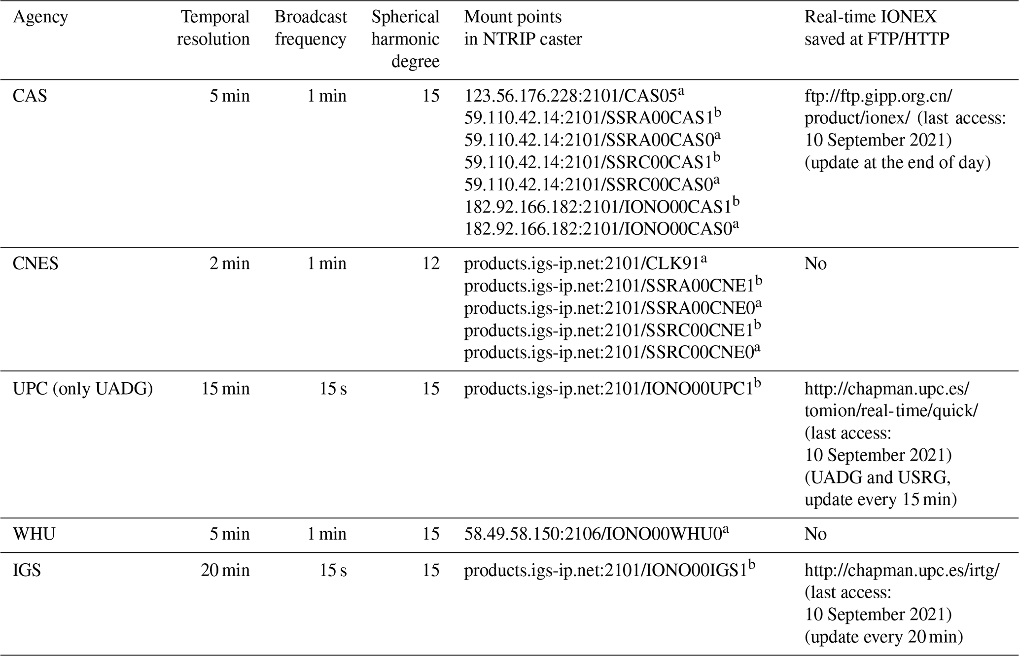
a RTCM-SSR format.
b IGS-SSR format.

Figure 1The 25 common real-time stations for RT-dSTEC assessment (in green) and 50 external GNSS stations for dSTEC-GPS assessment (in red).
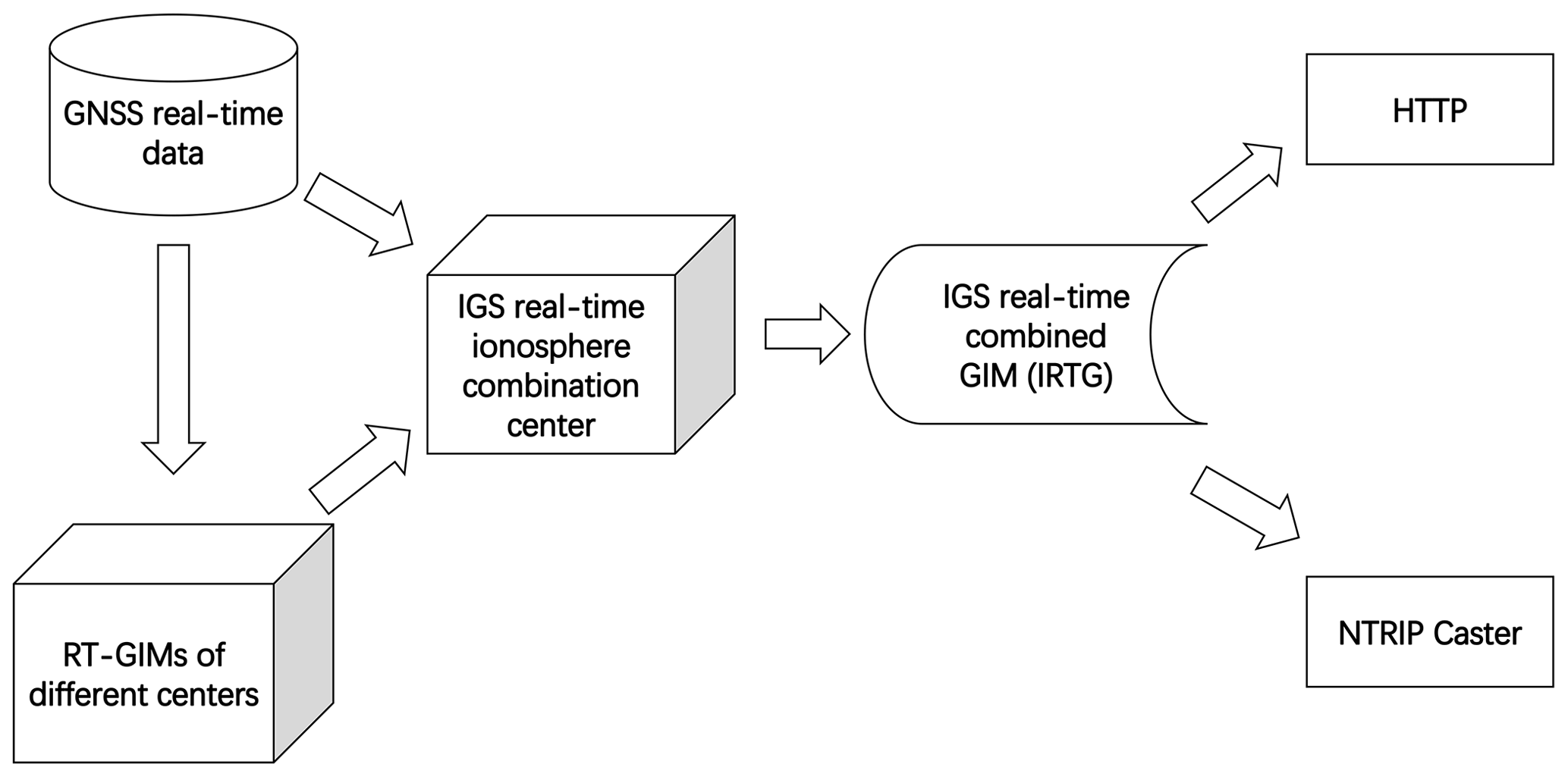
Due to the limited number of real-time stations, 25 common real-time stations that have been used by all the IGS real-time ionosphere centers are selected for allowing a fair RT-dSTEC assessment. The distribution can be seen as Fig. 1. Therefore, the RT-dSTEC is the measurement of “internal” post-fit residuals of RT-GIMs and still sensitive to the accuracy of assessed GIMs. Every 20 min, the RT-dSTEC assessment is performed and used for the combination of different IGS RT-GIMs. The steps for the generation of IRTG can be seen as Fig. 2. The RTCM-SSR has been the standard message for real-time corrections, and the IGS State Space Representation (SSR) format version 1.00 was published on 5 October 2020 (IGS, 2020). The content of IGS-SSR is compatible with RTCM-SSR contents. And the IGS-SSR format can support more extensions such as satellite attitude, phase center offsets, and variations in the near future. At present, both RTCM-SSR and IGS-SSR formats are used for the dissemination of RT-GIMs. In addition, IGS defines different references for antenna correction: average phase center (APC) and center of mass (CoM). The current status of RT-GIMs from different ionosphere centers can be seen in Table 2. It should be noted that “SSRA” means the SSR with the APC reference, and “SSRC” means the SSR with the CoM reference.
In this section, the performance of IGS RT-GIMs was analyzed and compared with rapid IGS GIMs as well as IGS combined final GIM. It should be noted that the RT-GIMs were gathered with BKG Ntrip Client (BNC) software (Weber et al., 2016) and generated by received spherical harmonic coefficients from different centers as in Table 2. And there were two kinds of temporal resolution for received RT-GIMs: the common temporal resolution of 20 min and the full (original) temporal resolution. Since the IRTG is combined every 20 min, we will focus on such a common time resolution to compare the performance. The detail of compared RT-GIMs can be seen in Table 3. The influence of temporal resolution on RT-GIMs was also shown in this section.
Table 3The ID of compared IGS RT-GIMs.
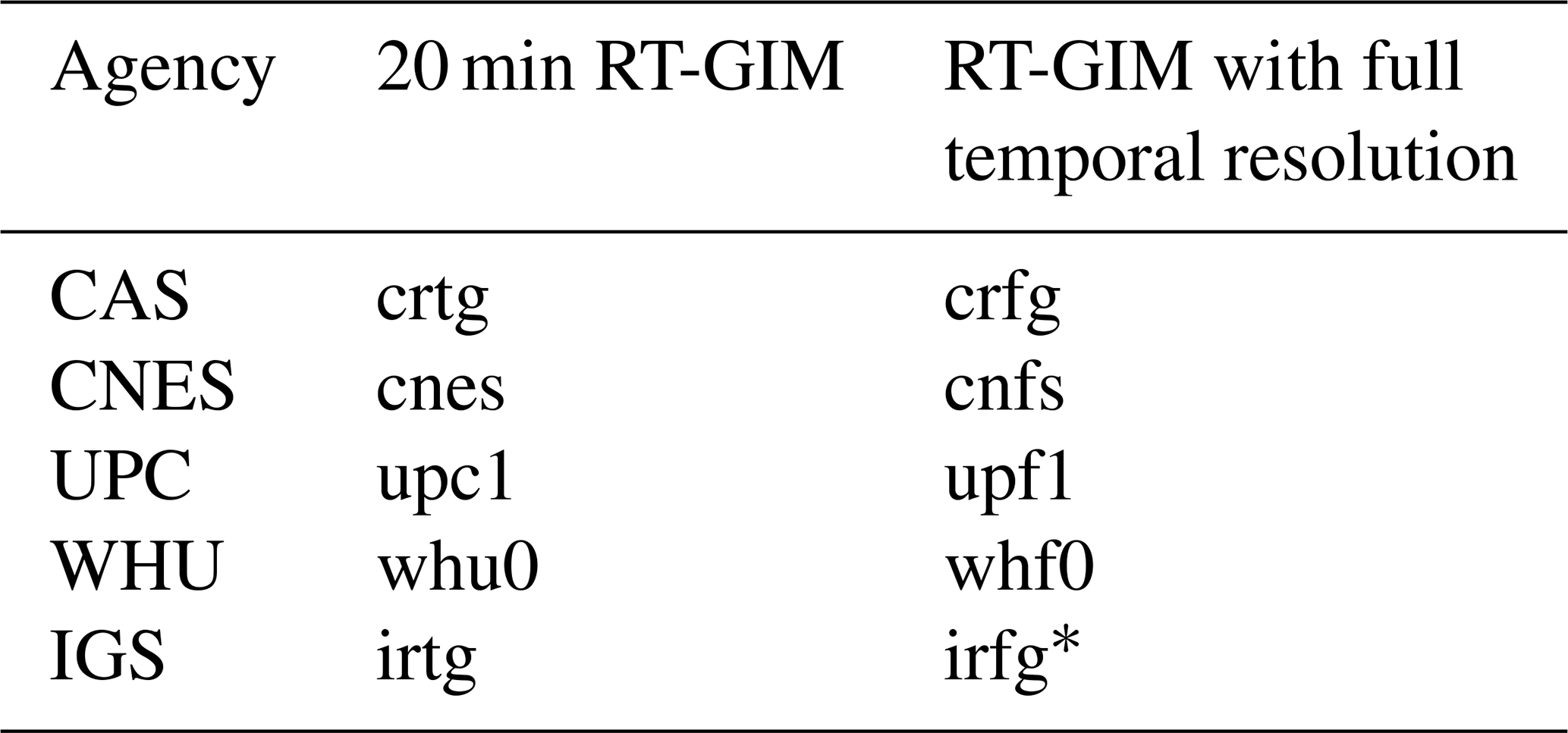
* Note irfg and irtg are the same.
Before detailing the Jason-3 VTEC and GPS-dSTEC assessment, it should be taken into account that the GIM error versus Jason VTEC measurements have a high correlation with the GIM error versus dSTEC-GPS measurements, although the Jason VTEC measurements are vertical and the dSTEC-GPS measurements are slanted. As demonstrated in Hernández-Pajares et al. (2017), the Jason-3 VTEC assessment and dSTEC-GPS assessment are independent and consistent for GIM evaluation. In other words, the slant ray path geometry changes do not affect the capability of dSTEC reference data to rank the GIM, and the electron content between the Jason-3 altimeter and the GNSS satellites does not significantly affect the assessment of GIMs based on Jason-3 VTEC data.
3.1 Jason-3 VTEC assessment
The VTEC from the Jason-3 altimeter was gathered as an external reference over the oceans. After applying a sliding window of 16 s to smooth the altimeter measurements, the typical standard deviation of Jason-3 VTEC measurement error is around 1 TECU. Although the electron content above the Jason-3 altimeter (about 1300 km) is not available and the altimeter bias is around a few TECU, the standard deviation of the difference between GIM-VTEC and Jason-3 VTEC is adopted to avoid the Jason-3 altimeter bias and the constant bias component of the plasmaspheric electron content in the assessment. The plasmaspheric electron content variation is up to a few TECU and is a relatively small part when compared with the GIM errors over the oceans. Jason-3 VTEC has been proven to be a reliable reference of VTEC over the oceans. The oceans are the most challenging regions for GIMs where permanent GNSS receivers are typically far away (Roma-Dollase et al., 2018b; Hernández-Pajares et al., 2017). In this context, the daily standard deviation of the difference between Jason-3 VTEC and GIM-VTEC was suitable as the statistic for GIM assessment in Eq. (9).
where VTECJason,i and VTECGIM,i are VTEC extracted from Jason-3 and GIM observation i, respectively. NJ is the number of involved observations.
The recent 3-month data (1 December 2020 to 1 March 2021), containing the two significant events (new contributing RT-GIM (WHU) from 3 January 2021 and the introduction of the new atomic decomposition UPC-GIM (UADG) on 4 January 2021), have been selected to study the consistency and performance of the IGS RT-GIMs.
As can be seen in Fig. 3, the standard deviation of UPC RT-GIM (upc1) VTEC versus measured Jason-3 VTEC is worse than other RT-GIMs before the transition from USRG to UADG on 4 January 2021. It should be noted that the upc1 in RTCM-SSR format was stopped from 15 December 2020 to 2 January 2021, due to the change of broadcasting format and some technical issues. The assessment of upc1 was based on the UPC RT-GIMs saved in a local repository during the interrupted period. The standard deviation of upc1 VTEC versus measured Jason-3 VTEC reached around 7 TECU on 6 December 2020 due to the interruption of the downloading module. And the upc1 achieved a significant improvement after the transition on 4 January 2021. In addition, the accuracy of IGS experimental combined RT-GIM (irtg) also increased due to the better performance of upc1. Compared with IGS rapid GIMs (corg, ehrg, emrg, esrg, igrg, jprg, uhrg, uprg, uqrg, whrg) and IGS final combined GIM (igsg), the upc1 and irtg are equivalent to the post-processed GIMs and even better than some rapid GIMs. The accuracy of CAS RT-GIM (crtg) and CNES RT-GIM (cnes) is close to the post-processed GIMs, while WHU RT-GIM (whu0) is slightly worse than the other GIMs. As shown and explained in Eq. (4), the whu0 is shifted by 0 h. To see the influence of phase-shifted λS,t, the whu0 is manually shifted by 2 h (i.e., take t0 as 2 h for whu0 in Eq. 4) in post-processing mode. And the accuracy of the 2 h shifted WHU RT-GIM (whu1) is slightly better than whu0 as can be seen in Fig. 3.
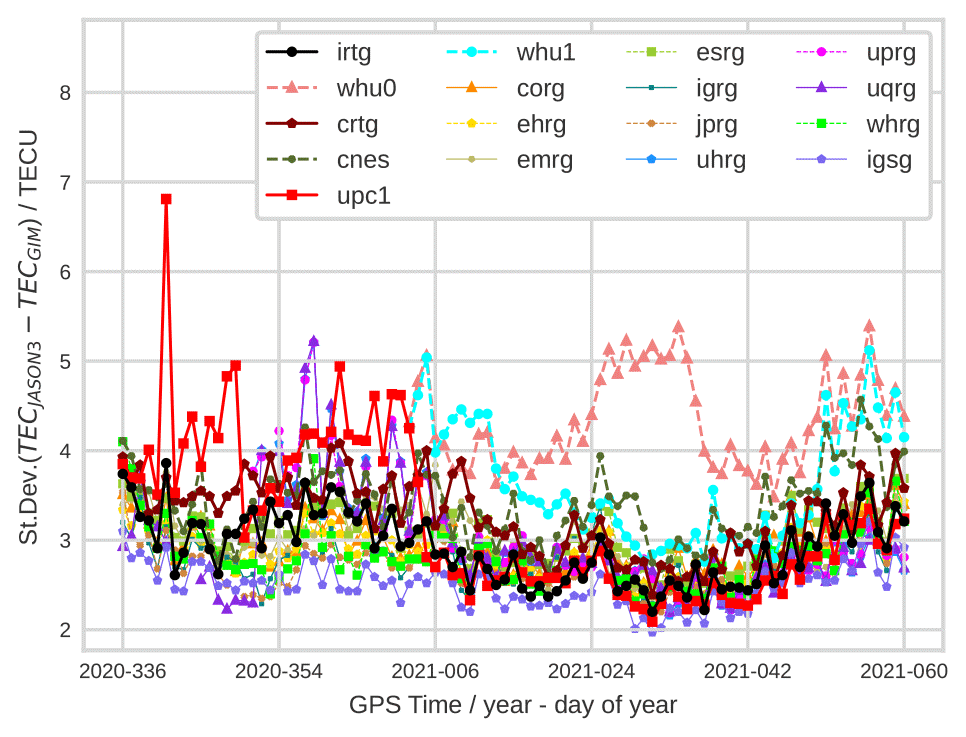
Figure 3Daily standard deviation of GIM VTEC versus measured Jason-3 VTEC (in TECU), from 1 December 2020 to 1 March 2021.
Table 4Standard deviation of GIM-VTEC minus Jason-3 VTEC in Jason-3 VTEC assessment (last two columns) and dSTEC-GPS assessment results of RT-GIMs on 3 January (second and third columns) and 5 January (fourth and fifth columns) in 2021.
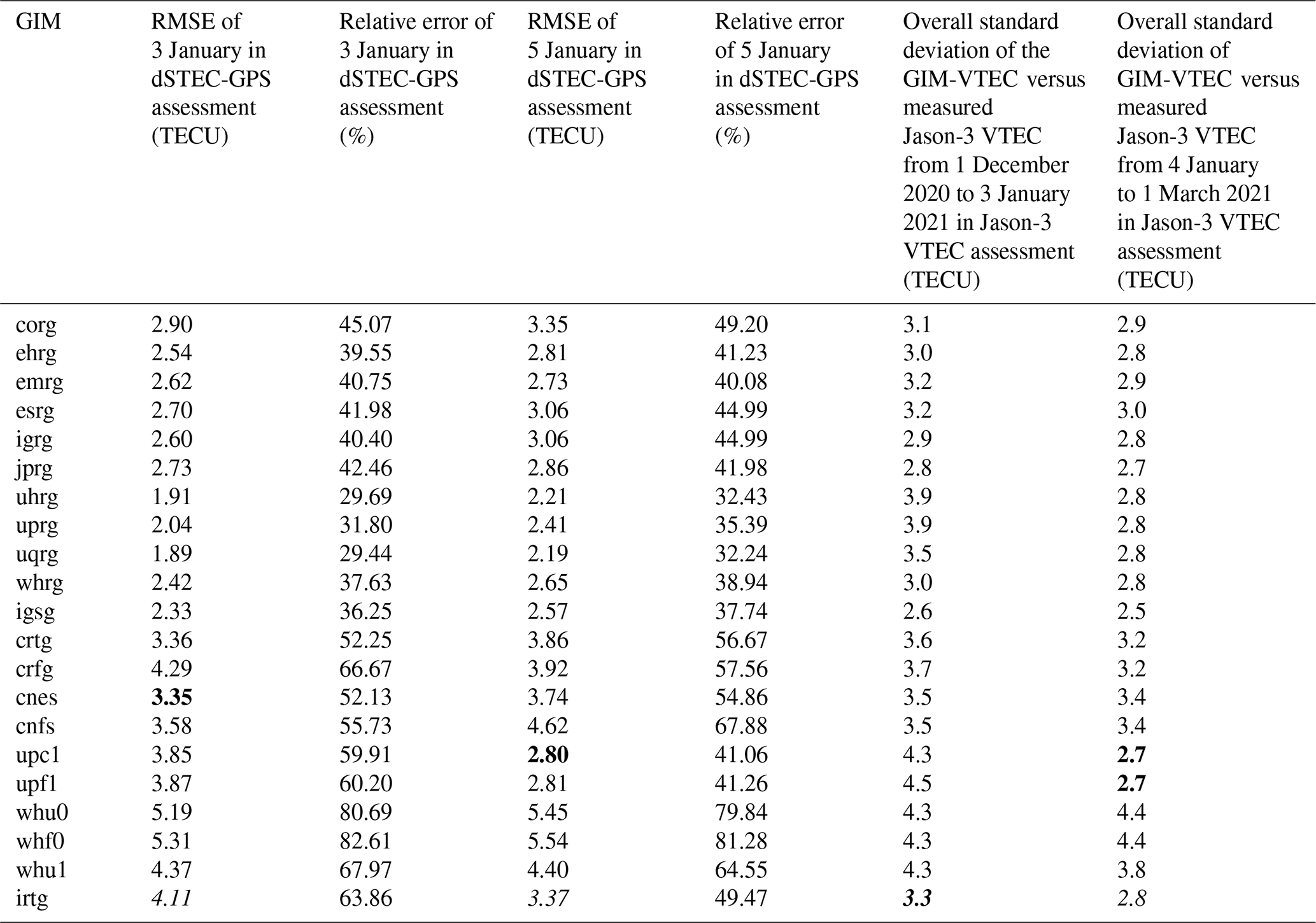
The value in bold font means the corresponding RT-GIM has the best performance among the remaining RT-GIMs in each column, and values of irtg are italic for comparison.
In order to investigate the influence of temporal resolution on RT-GIMs over oceans, different RT-GIMs with full temporal resolution were involved. The summary of Jason-3 VTEC assessment can be seen in Table 4. The overall standard deviation of GIM-VTEC minus Jason-3 VTEC is computed in separate time periods to focus on the influence of the transition from USRG to UADG. As shown in Table 4, the overall standard deviation of GIM-VTEC versus Jason-3 VTEC is consistent with Fig. 3, and the quality of 20 min and full temporal resolution of RT-GIMs are similar over oceans. And the accuracy of 2 h shifted whu1 in Jason-3 VTEC assessment is higher than whu0 in Table 4. In particular, the overall standard deviation of upc1 VTEC versus measured Jason-3 VTEC drops from 4.3 to 2.7 TECU, and, in agreement with that, the standard deviation of irtg VTEC versus measured Jason-3 VTEC decreases from 3.3 to 2.8 TECU.
3.2 dSTEC-GPS assessment
In addition, dSTEC-GPS assessment in post-processing mode was involved as a complementary tool with high accuracy (better than 0.1 TECU) over continental regions on a global scale. In the dSTEC-GPS assessment, the maximum elevation angle within a continuous arc was regarded as the reference angle in Eq. (8). The dSTEC observations provide the direct measurements of the difference of STEC within a continuous phase arc involving different geometries. As has been introduced before, the STEC is proportional to VTEC by means of the ionospheric mapping function. Therefore, the dSTEC error observations (see Eq. 8), containing different geometries and mapping function error are direct measurements for evaluating GIM-STEC, which is commonly used by GNSS users to calculate ionospheric correction. In addition, the common agreed ionospheric thin layer model is set to be 450 km in height in the generation of GIM to provide VTEC in a consistent way for different ionospheric analysis centers. And in this way the GNSS users are able to consistently recover the STEC from GIM-VTEC by the commonly agreed mapping function. The dSTEC-GPS assessment was performed by globally distributed GNSS stations as shown in Fig. 1 on 3 January (before the transition of UPC RT-GIM from USRG to UADG) and 5 January (after the transition) in 2021, with a focus on the transition of UPC RT-GIM. The rms error and relative error were used for the assessment as Eq. (10).
Here RMSδ,g is the rms error of GIM g. And δg,i is the dSTEC error of GIM g similar to Eq. (8), while the reference angle of Eq. (8) is replaced by the maximum elevation angle within a continuous arc. NS is the number of involved observations. is the dSTEC-GPS observation. is the rms of the observed dSTEC-GPS. Relative errorg is the relative error of GIM g.
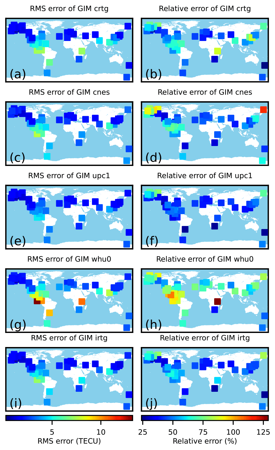
Figure 4The distribution of dSTEC-GPS results on 5 January 2021 (after the improvement of the UPC interpolation technique).
As shown in Table 4, the rms error of most post-processed GIMs reaches around 2 or 3 TECU, while the rms error ranges from 2.8 to 5.54 TECU for RT-GIMs. The transition of UPC RT-GIM (upf1) from USRG to UADG is apparent in the dSTEC-GPS assessment, and the rms error of IGS RT-GIM (irtg) decreased from 4.11 to 3.37 TECU due to the improvement of UPC RT-GIM. After the transition of UPC RT-GIM, the performance of upf1 and irtg is comparable with most post-processed GIMs. Similar to the performance in the Jason-3 VTEC assessment, the accuracy of the remaining RT-GIMs is close to post-processed GIMs. And the rms error of 2 h shifted whu1 is around 4.4 TECU, which is better than the whu0. Therefore, the 2 h shift is recommended for λS,t in Eq. (4). It should be pointed out that the performance of RT-GIMs with the full temporal resolution is slightly worse than 20 min RT-GIMs. Furthermore, the full temporal resolution RT-GIM is even worse than the GIM obtained by linear interpolation of the 20 min RT-GIM in a sun-fixed reference frame. This is coincident with a smaller number of ionospheric observations at shorter timescales. In Fig. 4, the performance of IGS RT-GIMs after the upgrade of the UPC interpolation method in the dSTEC-GPS assessment is represented. The higher values of rms errors occur around the Equator and Southern Hemisphere for all the RT-GIMs. And the higher values might be caused by the high-electron-density gradients at the Equator and the sparse distribution of real-time stations in the Southern Hemisphere.
3.3 The sensibility of real-time weighting technique
RT-dSTEC assessment of RT-GIMs was automatically running in real-time mode and used for real-time weighting in the combination of IGS RT-GIMs. In order to compare with the dSTEC-GPS assessment, the RT-dSTEC assessment with real-time stations in Fig. 1 was also performed on 3 and 5 January 2021. As can be seen in Table 5, the rank of RT-GIMs in the RT-dSTEC assessment is similar to the dSTEC-GPS assessment, but the rms error values are larger. And the larger rms error coincides with the much lower elevation angle of the observation reference in the RT-dSTEC assessment.
Table 5RMSE of RT-GIMs in RT-dSTEC assessment on 3 and 5 January 2021.
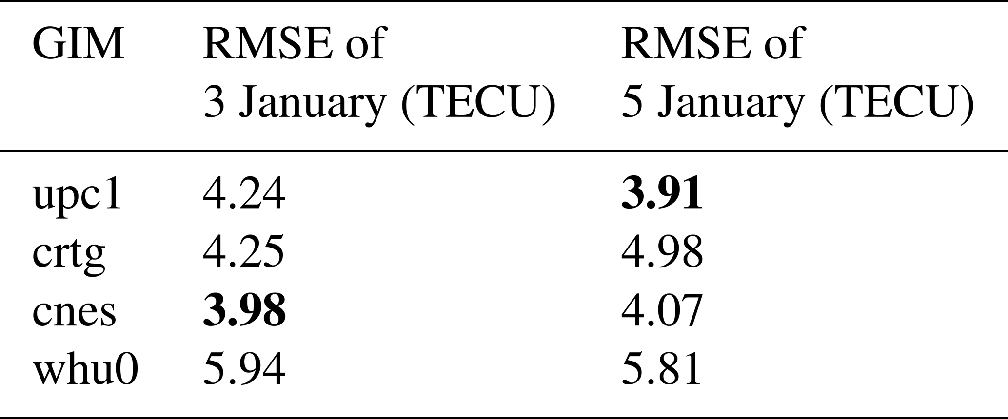
The value in bold font means the corresponding RT-GIM has the best performance among the remaining RT-GIMs in each column.

Figure 5The evolution of real-time weights and daily winning epochs of RT-GIMs. (a) The real-time weights from 3 to 5 January 2021. (b) The daily number of epochs when one of the RT-GIMs is better than the others from 1 December 2020 to 1 March 2021.
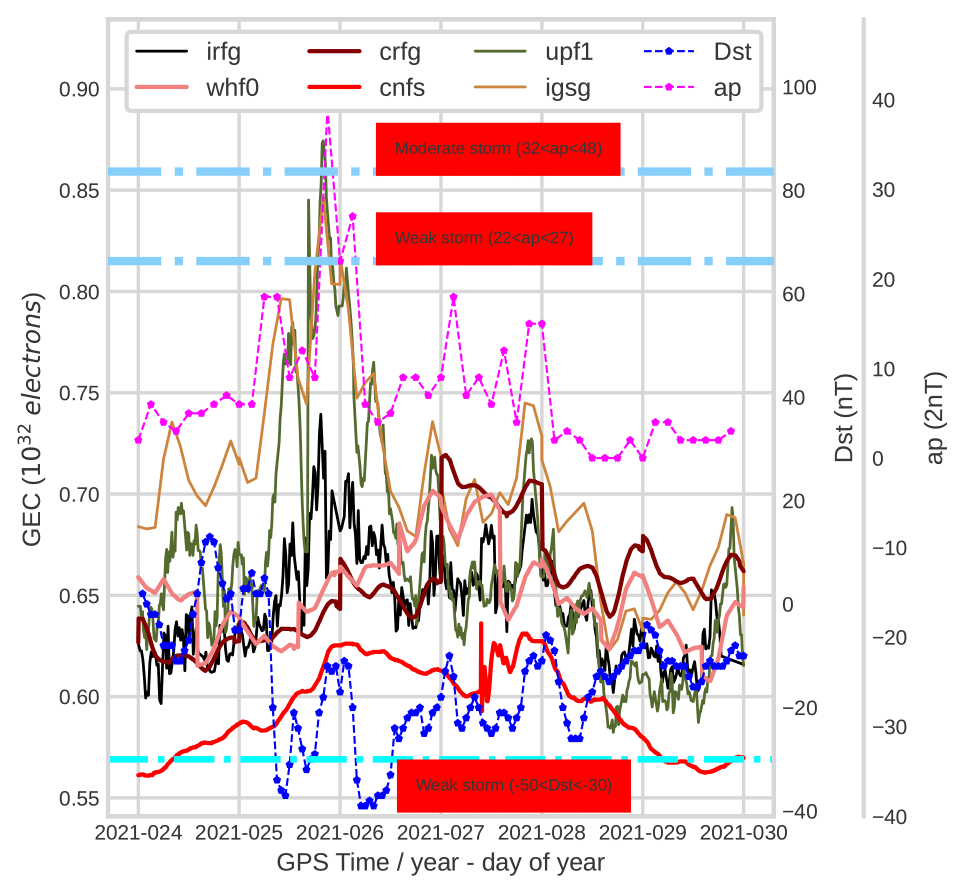
Figure 6The GEC, ap and Dst evolution of RT-GIMs from 24 to 29 January 2021 during the low-solar-activity period.
The real-time weights of RT-GIMs can be defined as the normalized inverse of the squared rms of RT-dSTEC errors and represent the accuracy of RT-GIMs in the RT-dSTEC assessment. For each RT-GIM, the number of daily winning epochs is computed by counting the number of epochs within the day when the one RT-GIM is better than the other RT-GIMs. The evolution of daily winning epochs of RT-GIMs shown in the bottom figure of Fig. 5 is consistent with the Jason-3 VTEC assessment. The upc1 was not involved in the combination from 15 December 2020 to 2 January 2021 when the dissemination of upc1 was stopped, as can be seen in the bottom figure of Fig. 5. The significant improvement of the transition of upc1 from USRG to UADG shown in dSTEC-GPS and the Jason-3 VTEC assessment is also obvious in the top panel of Fig. 5. In addition, the daily winning epoch's evolution and the transition in Fig. 5 are consistent with the accuracy of RT-GIMs, providing a combined RT-GIM which is one of the best RT-GIMs, as shown in the altimeter-based and dSTEC-based assessments. The good performance of the combination algorithm can be mainly explained from the point of view of the weights, i.e., the sensitivity of the dSTEC error to the quality of the RT-GIMs, but also from the point of view of the linear combination that can play a positive role under any potential negative correlation between the performance of pairs of involved RT-GIMs.
3.4 The response of RT-GIMs to recent minor geomagnetic storms
The global electron content (GEC) is defined as the total number of free electrons in the ionosphere. Hence the GEC can be estimated from the summation of the product of the VTEC value and the area of the corresponding GIM cell. In addition, GEC has been used as an ionospheric index (Afraimovich et al., 2006; Hernández-Pajares et al., 2009). With the purpose of further checking the consistency of IGS RT-GIMs, the GEC of RT-GIMs was calculated and compared from 24 to 29 January 2021. It should be noted that the solar activity is low in January 2021. During the selected period, several weak geomagnetic storms and one moderate geomagnetic storm occurred according to the classification of geomagnetic indices (Loewe and Prölss, 1997; Gonzalez et al., 1999), and the GEC evolution can be seen in Fig. 6. The GEC of CNES RT-GIM (cnfs) is slightly different from other RT-GIMs, and seems to be caused by the bias in CNES RT-GIM. There are some jumps in the GEC evolution of CAS RT-GIM (crfg) and WHU RT-GIM (whf0), and the jumps might be related to the handling of day boundary or unreal predicted GIM in certain cases. Compared with IGS final combined GIM (igsg), the good performance of global VTEC representation with upf1 and irfg can be seen in Fig. 6. In addition, the response of upf1 and irfg to the recent minor geomagnetic storms (detected by 3 h ap and 1 h Dst indices) is apparent and also similar to the post-processed IGS final combined GIM (igsg).
The IGS real-time combined GIMs during the testing period are available from Zenodo at https://doi.org/10.5281/zenodo.5042622 (Liu et al., 2021b) in IONEX format (Schaer et al., 1998). In addition, more archived IGS combined RT-GIMs can be found at http://chapman.upc.es/irtg/archive/ (Liu and Hernández-Pajares, 2021a), and the latest IGS combined RT-GIMs are available in real-time mode at http://chapman.upc.es/irtg/last_results/ (Liu and Hernández-Pajares, 2021b).
In this paper, we have summarized the computation methods of RT-GIMs from four individual IGS ionosphere centers and introduced the new version of IGS combined RT-GIM. According to the results of Jason-3 VTEC and dSTEC-GPS assessment, it could be concluded as follows.
-
The real-time weighting technique for the generation of IGS combined RT-GIM performs well when it is compared with Jason-3 VTEC and dSTEC-GPS assessment.
-
The transition of UPC RT-GIM from USRG to UADG is obvious in all involved assessments and also demonstrates the sensibility of the real-time weighting technique to RT-GIMs when the accuracy of RT-GIMs is increased.
-
The quality of most IGS RT-GIMs is close to post-processed GIMs.
-
The difference among RT-GIMs with 20 min and full temporal resolution can be neglected over oceans in the Jason-3 VTEC assessment (see Fig. 3 and Table 4), while the difference is visible in some RT-GIMs over continental regions in the dSTEC-GPS assessment (see Table 4). The lower accuracy of GIMs with full temporal resolution (2 or 5 min) might be related to the uneven distribution of ionospheric observations, the weight between predicted GIMs and real-time observations. Combined with the previous study (Liu et al., 2021a), it is suggested to find a more suitable temporal resolution for the generation of RT-GIM in a sun-fixed reference frame.
In addition, the GEC evolution of UPC RT-GIM and IGS combined RT-GIM is close to the GEC evolution of IGS final combined GIM in post-processing mode and has an obvious response to the geomagnetic storm during the low-solar-activity period. Future improvements might include the following.
-
Broadcast real-time rms maps that can be useful for the positioning users.
-
Increase the accuracy of high-temporal-resolution RT-GIMs. In addition, higher maximum spherical harmonic degrees might be adopted to increase the accuracy and spatial resolution of RT-GIMs.
-
Coinciding with a much larger number of RT-GNSS receivers in the future, the dSTEC weighting might be improved by replacing the “internal” with the “external” receivers, i.e., not used by any real-time analysis centers. In this way the weighting would be sensitive as well to the interpolation–extrapolation error of the different real-time ionospheric GIMs to be combined. And the resulting combination might behave better.
-
Increase the number of worldwide GNSS receivers used for the RT-dSTEC up to more than 100. In this way we will be able to study the potential upgrade of the present global weighting to a regional weighting among other potential improvements in the combination strategy.
QL wrote the manuscript. QL developed the updated combination software with contributions from DRD, HY and MHP. QL and MHP designed the research, with contributions from HY, EMM, DRD and AGR. QL, HY, EMM, MHP, ZL, NW, DL, AB, Q. Zhao and Q. Zhang provided the real-time GIMs of the corresponding IGS centers. AH, MS, GW and AS contributed in creating the framework of the real-time IGS service, the ionospheric message format and BNC open software updates. LA suggested the initial idea of this work. AK, StS, JF, AK, RGF and AGR contributed in the generation of rapid and final IGS GIMs used as additional references in the manuscript.
The contact author has declared that neither they nor their co-authors have any competing interests.
Publisher's note: Copernicus Publications remains neutral with regard to jurisdictional claims in published maps and institutional affiliations.
The authors are thankful to the collaborative and friendly framework of the International GNSS Service, an organization providing first-class open data and open products (Johnston et al., 2017). The VTEC data from the Jason-3 altimeter were gathered from the NASA EOSDIS Physical Oceanography Distributed Active Archive Center (PO.DAAC) at the Jet Propulsion Laboratory, Pasadena, CA (https://doi.org/10.5067/GHGMR-4FJ01), and the National Oceanic and Atmospheric Administration (NOAA). We are also thankful to GeoForschungsZentrum (GFZ) and to World Data Center (WDC) for Geomagnetism, Kyoto, for providing the ap and Dst indices.
This research has been supported by the China Scholarship Council (CSC). The contribution from UPC-IonSAT authors was partially supported by the European Union-funded project PITHIA-NRF (grant no. 101007599) and by the ESSP/ICAO-funded project TEC4SpaW. The work of Andrzej Krankowski is supported by the National Centre for Research and Development, Poland, through grant ARTEMIS (grant nos. DWM/PL-CHN/97/2019 and WPC1/ARTEMIS/2019).
This paper was edited by Christian Voigt and reviewed by two anonymous referees.
Afraimovich, E., Astafyeva, E., Oinats, A., Yasukevich, Y. V., and Zhivetiev, I.: Global electron content and solar activity: comparison with IRI modeling results, in: poster presentation at IGS Workshop, Darmdstadt, Germany, 8–11 May 2006. a
Caissy, M., Agrotis, L., Weber, G., Hernandez-Pajares, M., and Hugentobler, U.: Innovation: Coming Soon-The International GNSS Real-Time Service, available at: https://www.gpsworld.com/gnss-systemaugmentation-assistanceinnovation-coming-soon-13044/ (last access: 21 March 2021), 2012. a
Chen, J., Ren, X., Zhang, X., Zhang, J., and Huang, L.: Assessment and Validation of Three Ionospheric Models (IRI-2016, NeQuick2, and IGS-GIM) From 2002 to 2018, Space Weather, 18, e2019SW002422, https://doi.org/10.1029/2019SW002422, 2020. a
Ciraolo, L., Azpilicueta, F., Brunini, C., Meza, A., and Radicella, S.: Calibration errors on experimental slant total electron content (TEC) determined with GPS, J. Geodesy, 81, 111–120, https://doi.org/10.1007/s00190-006-0093-1, 2007. a
Elsobeiey, M. and Al-Harbi, S.: Performance of real-time Precise Point Positioning using IGS real-time service, GPS Solut., 20, 565–571, https://doi.org/10.1007/s10291-015-0467-z, 2016. a
Feltens, J.: Development of a new three-dimensional mathematical ionosphere model at European Space Agency/European Space Operations Centre, Space Weather, 5, S12002, https://doi.org/10.1029/2006SW000294, 2007. a
Feltens, J. and Schaer, S.: IGS Products for the Ionosphere, in: Proceedings of the 1998 IGS Analysis Center Workshop Darmstadt, Germany, 9–11 February 1998, pp. 3–5, 1998. a
Fernandes, M. J., Lázaro, C., Nunes, A. L., and Scharroo, R.: Atmospheric corrections for altimetry studies over inland water, Remote Sens.-Basel, 6, 4952–4997, https://doi.org/10.3390/rs6064952, 2014. a
Froń, A., Galkin, I., Krankowski, A., Bilitza, D., Hernández-Pajares, M., Reinisch, B., Li, Z., Kotulak, K., Zakharenkova, I., Cherniak, I., Roma Dollase, D., Wang, N., Flisek, P., and García-Rigo, A.: Towards Cooperative Global Mapping of the Ionosphere: Fusion Feasibility for IGS and IRI with Global Climate VTEC Maps, Remote Sens.-Basel, 12, 3531, https://doi.org/10.3390/rs12213531, 2020. a
García-Rigo, A., Monte, E., Hernández-Pajares, M., Juan, J., Sanz, J., Aragón-Angel, A., and Salazar, D.: Global prediction of the vertical total electron content of the ionosphere based on GPS data, Radio Sci., 46, RS0D25, https://doi.org/10.1029/2010RS004643, 2011. a
García Rigo, A., Roma Dollase, D., Hernández Pajares, M., Li, Z., Terkildsen, M., Ghoddousi Fard, R., Dettmering, D., Erdogan, E., Haralambous, H., Beniguel, Y., Berdermann, J., Kriegel, M., Krypiak-Gregorczyk, A., Gulyaeva, T., Komjathy, A., Vergados, P., Feltens, J., Zandbergen, R., Olivares, G., Fuller-Rowell, T., Altadill, D., Blanch, E., Bergeot, N., Krankowski, A., Agrotis, L., Galkin, I., Orus-Perez, R., and Prol, F. S.: St. Patrick's day 2015 geomagnetic storm analysis based on real time ionosphere monitoring, in: EGU 2017: European Geosciences Union General Assembly, Vienna, Austria, 23–28 April 2017, proceedings book, 2017. a
Ghoddousi-Fard, R.: GPS ionospheric mapping at Natural Resources Canada, in: IGS workshop, Pasadena, 23–27 June 2014. a
Gonzalez, W. D., Tsurutani, B. T., and De Gonzalez, A. L. C.: Interplanetary origin of geomagnetic storms, Space Sci. Rev., 88, 529–562, https://doi.org/10.1023/A:1005160129098, 1999. a
Gulyaeva, T. L. and Stanislawska, I.: Derivation of a planetary ionospheric storm index, Ann. Geophys., 26, 2645–2648, https://doi.org/10.5194/angeo-26-2645-2008, 2008. a
Gulyaeva, T. L., Arikan, F., Hernandez-Pajares, M., and Stanislawska, I.: GIM-TEC adaptive ionospheric weather assessment and forecast system, J. Atmos. Sol.-Terr. Phy., 102, 329–340, https://doi.org/10.1016/j.jastp.2013.06.011, 2013. a
Hernández-Pajares, M., Juan, J., and Sanz, J.: Neural network modeling of the ionospheric electron content at global scale using GPS data, Radio Sci., 32, 1081–1089, https://doi.org/10.1029/97RS00431, 1997. a
Hernández-Pajares, M., Juan, J., Sanz, J., and Solé, J.: Global observation of the ionospheric electronic response to solar events using ground and LEO GPS data, J. Geophys. Res.-Space, 103, 20789–20796, https://doi.org/10.1029/98JA01272, 1998. a, b
Hernández-Pajares, M., Juan, J., and Sanz, J.: New approaches in global ionospheric determination using ground GPS data, J. Atmos. Sol.-Terr. Phy., 61, 1237–1247, https://doi.org/10.1016/S1364-6826(99)00054-1, 1999. a, b, c
Hernández-Pajares, M., Juan, J., Sanz, J., Orus, R., García-Rigo, A., Feltens, J., Komjathy, A., Schaer, S., and Krankowski, A.: The IGS VTEC maps: a reliable source of ionospheric information since 1998, J. Geodesy, 83, 263–275, https://doi.org/10.1007/s00190-008-0266-1, 2009. a, b, c
Hernández-Pajares, M., Roma-Dollase, D., Krankowski, A., García-Rigo, A., and Orús-Pérez, R.: Methodology and consistency of slant and vertical assessments for ionospheric electron content models, J. Geodesy, 91, 1405–1414, https://doi.org/10.1007/s00190-017-1032-z, 2017. a, b
Hernández-Pajares, M., Lyu, H., Aragón-Àngel, À., Monte-Moreno, E., Liu, J., An, J., and Jiang, H.: Polar Electron Content From GPS Data-Based Global Ionospheric Maps: Assessment, Case Studies, and Climatology, J. Geophys. Res.-Space, 125, e2019JA027677, https://doi.org/10.1029/2019JA027677, 2020. a
Hoque, M. M., Jakowski, N., and Orús-Pérez, R.: Fast ionospheric correction using Galileo Az coefficients and the NTCM model, GPS Solut., 23, 41, https://doi.org/10.1007/s10291-019-0833-3, 2019. a
IGS: IGS State Space Representation (SSR) Format Version 1.00, available at: https://files.igs.org/pub/data/format/igs_ssr_v1.pdf (last access: 21 March 2021), 2020. a, b
Jakowski, N., Hoque, M., and Mayer, C.: A new global TEC model for estimating transionospheric radio wave propagation errors, J. Geodesy, 85, 965–974, https://doi.org/10.1007/s00190-011-0455-1, 2011. a
Jiang, H., Liu, J., Wang, Z., An, J., Ou, J., Liu, S., and Wang, N.: Assessment of spatial and temporal TEC variations derived from ionospheric models over the polar regions, J. Geodesy, 93, 455–471, https://doi.org/10.1007/s00190-018-1175-6, 2019. a
Johnston, G., Riddell, A., and Hausler, G.: The International GNSS Service, in: Springer Handbook of Global Navigation Satellite Systems, 1st edn., edited by: Teunissen, P. J. and Montenbruck, O., Springer International Publishing, Cham, Switzerland, 967–982, https://doi.org/10.1007/978-3-319-42928-1, 2017. a
Komjathy, A. and Born, G. H.: GPS-based ionospheric corrections for single frequency radar altimetry, J. Atmos. Sol.-Terr. Phy., 61, 1197–1203, https://doi.org/10.1016/S1364-6826(99)00051-6, 1999. a
Komjathy, A., Galvan, D., Stephens, P., Butala, M., Akopian, V., Wilson, B., Verkhoglyadova, O., Mannucci, A., and Hickey, M.: Detecting ionospheric TEC perturbations caused by natural hazards using a global network of GPS receivers: The Tohoku case study, Earth Planets Space, 64, 1287–1294, https://doi.org/10.5047/eps.2012.08.003, 2012. a
Laurichesse, D. and Blot, A.: New CNES real time products including BeiDou, available at: https://lists.igs.org/pipermail/igsmail/2015/001017.html (last access: 21 March 2021), 2015. a, b
Le, A. Q. and Tiberius, C.: Single-frequency precise point positioning with optimal filtering, GPS Solut., 11, 61–69, https://doi.org/10.1007/s10291-006-0033-9, 2007. a
Li, M., Yuan, Y., Wang, N., Li, Z., and Huo, X.: Performance of various predicted GNSS global ionospheric maps relative to GPS and JASON TEC data, GPS Solut., 22, 55, https://doi.org/10.1007/s10291-018-0721-2, 2018. a
Li, X., Ge, M., Zhang, H., and Wickert, J.: A method for improving uncalibrated phase delay estimation and ambiguity-fixing in real-time precise point positioning, J. Geodesy, 87, 405–416, https://doi.org/10.1007/s00190-013-0611-x, 2013. a
Li, Z., Yuan, Y., Wang, N., Hernandez-Pajares, M., and Huo, X.: SHPTS: towards a new method for generating precise global ionospheric TEC map based on spherical harmonic and generalized trigonometric series functions, J. Geodesy, 89, 331–345, https://doi.org/10.1007/s00190-014-0778-9, 2015. a, b
Li, Z., Wang, N., Hernández Pajares, M., Yuan, Y., Krankowski, A., Liu, A., Zha, J., García Rigo, A., Roma-Dollase, D., Yang, H., Laurichesse, D., and Blot, A.: IGS real-time service for global ionospheric total electron content modeling, J. Geodesy, 94, 32, https://doi.org/10.1007/s00190-020-01360-0, 2020. a, b, c, d, e, f
Liu, J.-Y., Chen, Y., Chuo, Y., and Chen, C.-S.: A statistical investigation of preearthquake ionospheric anomaly, J. Geophys. Res.-Space, 111, A05304, https://doi.org/10.1029/2005JA011333, 2006. a
Liu, L., Wan, W., Ning, B., and Zhang, M.-L.: Climatology of the mean total electron content derived from GPS global ionospheric maps, J. Geophys. Res.-Space, 114, A06308, https://doi.org/10.1029/2009JA014244, 2009. a
Liu, Q. and Hernández-Pajares, M.: The archive of IGS combined real-time GIM [data set], available at: http://chapman.upc.es/irtg/archive, last access: 10 September 2021a. a
Liu, Q. and Hernández-Pajares, M.: The latest results of IGS combined real-time GIM [data set], available at: http://chapman.upc.es/irtg/last_results, last access: 10 September 2021b. a
Liu, Q., Hernández-Pajares, M., Lyu, H., and Goss, A.: Influence of temporal resolution on the performance of global ionospheric maps, J. Geodesy, 95, 34, https://doi.org/10.1007/s00190-021-01483-y, 2021a. a
Liu, Q., Hernández-Pajares, M., Yang, H., Monte-Moreno, E., Roma, D., García Rigo, A., Li, Z., Wang, N., Laurichesse, D., Blot, A., Zhao, Q., and Zhang, Q.: Global Ionosphere Maps of vertical electron content combined in real-time from the RT-GIMs of CAS, CNES, UPC-IonSAT, and WHU International GNSS Service (IGS) centers (from Dec 1, 2020, to March 1, 2021), Zenodo [data set], https://doi.org/10.5281/zenodo.5042622, 2021b. a, b
Loewe, C. and Prölss, G.: Classification and mean behavior of magnetic storms, J. Geophys. Res.-Space, 102, 14209–14213, https://doi.org/10.1029/96JA04020, 1997. a
Lou, Y., Zheng, F., Gu, S., Wang, C., Guo, H., and Feng, Y.: Multi-GNSS precise point positioning with raw single-frequency and dual-frequency measurement models, GPS Solut., 20, 849–862, https://doi.org/10.1007/s10291-015-0495-8, 2016. a
Mannucci, A., Wilson, B., Yuan, D., Ho, C., Lindqwister, U., and Runge, T.: A global mapping technique for GPS-derived ionospheric total electron content measurements, Radio Sci., 33, 565–582, https://doi.org/10.1029/97RS02707, 1998. a
Orús, R., Hernández-Pajares, M., Juan, J., and Sanz, J.: Improvement of global ionospheric VTEC maps by using kriging interpolation technique, J. Atmos. Sol.-Terr. Phy., 67, 1598–1609, https://doi.org/10.1016/j.jastp.2005.07.017, 2005. a
Ren, X., Chen, J., Li, X., Zhang, X., and Freeshah, M.: Performance evaluation of real-time global ionospheric maps provided by different IGS analysis centers, GPS Solut., 23, 113, https://doi.org/10.1007/s10291-019-0904-5, 2019. a
Roma-Dollase, D., Gómez Cama, J. M., Hernández Pajares, M., and García-Rigo, A.: Real-time Global Ionospheric modelling from GNSS data with RT-TOMION model, in: 5th International Colloquium Scientific and Fundamental Aspects of the Galileo Programme, Braunschweig, Germany, 27–29 October 2015. a
Roma-Dollase, D., Hernández-Pajares, M., García Rigo, A., Krankowski, A., Fron, A., Laurichesse, D., Blot, A., Orús-Pérez, R., Yuan, Y., Li, Z., Wang, N., Schmidt, M., and Erdogan, E.: Looking for optimal ways to combine global ionospheric maps in real-time, in: IGS workshop 2018, Wuhan, 29 October–2 November, 2018a. a, b
Roma-Dollase, D., Hernández-Pajares, M., Krankowski, A., Kotulak, K., Ghoddousi-Fard, R., Yuan, Y., Li, Z., Zhang, H., Shi, C., Wang, C., Feltens, J., Vergados, P., Komjathy, A., Schaer, S., García-Rigo, A., and Gómez-Cama, J. M.: Consistency of seven different GNSS global ionospheric mapping techniques during one solar cycle, J. Geodesy, 92, 691–706, https://doi.org/10.1007/s00190-017-1088-9, 2018b. a
RTCM-SC: Proposal of new RTCM SSR messages, SSR Stage 2: Vertical TEC (VTEC) for RTCM Standard 10403.2 Differential GNSS (global navigation satellite system) Services – Version 3, RTCM Special Committee, 104, 2014. a, b
Schaer, S., Beutler, G., Rothacher, M., and Springer, T. A.: Daily global ionosphere maps based on GPS carrier phase data routinely produced by the CODE Analysis Center, in: Proceedings of the IGS AC Workshop, Silver Spring, MD, USA, 19–21 March, 1996. a
Schaer, S., Gurtner, W., and Feltens, J.: IONEX: The ionosphere map exchange format version 1, in: Proceedings of the IGS AC workshop, Darmstadt, Germany, 9–11 February 1998, vol. 9, 1998. a, b
Sezen, U., Arikan, F., Arikan, O., Ugurlu, O., and Sadeghimorad, A.: Online, automatic, near-real time estimation of GPS-TEC: IONOLAB-TEC, Space Weather, 11, 297–305, https://doi.org/10.1002/swe.20054, 2013. a
Sotomayor-Beltran, C., Sobey, C., Hessels, J., De Bruyn, G. et al.: Calibrating high-precision Faraday rotation measurements for LOFAR and the next generation of low-frequency radio telescopes, Astron. Astrophys., 552, A58, https://doi.org/10.1051/0004-6361/201220728, 2013. a
Tange, O.: Gnu parallel-the command-line power tool, The USENIX Magazine, 36, 42–47, https://doi.org/10.5281/zenodo.16303, 2011. a
Tomaszewski, D., Wielgosz, P., Rapiński, J., Krypiak-Gregorczyk, A., Kaźmierczak, R., Hernández-Pajares, M., Yang, H., and OrúsPérez, R.: Assessment of Centre National d'Etudes Spatiales Real-Time Ionosphere Maps in Instantaneous Precise Real-Time Kinematic Positioning over Medium and Long Baselines, Sensors, 20, 2293, https://doi.org/10.3390/s20082293, 2020. a
Wang, N., Li, Z., Duan, B., Hugentobler, U., and Wang, L.: GPS and GLONASS observable-specific code bias estimation: comparison of solutions from the IGS and MGEX networks, J. Geodesy, 94, 74, https://doi.org/10.1007/s00190-020-01404-5, 2020. a
Weber, G., Mervart, L., Lukes, Z., Rocken, C., and Dousa, J.: Real-time clock and orbit corrections for improved point positioning via NTRIP, in: Proceedings of the 20th international technical meeting of the satellite division of the institute of navigation (ION GNSS 2007), Fort Worth, USA, 25–28 September 2007, pp. 1992–1998, 2007. a
Weber, G., Mervart, L., Stürze, A., Rülke, A., and Stöcker, D.: BKG Ntrip Client, Version 2.12, vol. 49 of Mitteilungen des Bundesamtes für Kartographie und Geodäsie, Verlag des Bundesamtes für Kartographie und Geodäsie, Frankfurt am Main, 2016. a
Wright, J., Yang, A. Y., Ganesh, A., Sastry, S. S., and Ma, Y.: Robust face recognition via sparse representation, IEEE T. Pattern Anal., 31, 210–227, https://doi.org/10.1109/TPAMI.2008.79, 2008. a
Wright, J., Ma, Y., Mairal, J., Sapiro, G., Huang, T. S., and Yan, S.: Sparse representation for computer vision and pattern recognition, P. IEEE, 98, 1031–1044, https://doi.org/10.1109/JPROC.2010.2044470, 2010. a
Yang, H., Monte-Moreno, E., Hernández-Pajares, M., and Roma-Dollase, D.: Real-time interpolation of global ionospheric maps by means of sparse representation, J. Geodesy, 95, 71, https://doi.org/10.1007/s00190-021-01525-5, 2021. a
Zhang, B., Teunissen, P. J., Yuan, Y., Zhang, X., and Li, M.: A modified carrier-to-code leveling method for retrieving ionospheric observables and detecting short-term temporal variability of receiver differential code biases, J. Geodesy, 93, 19–28, https://doi.org/10.1007/s00190-018-1135-1, 2019. a
Zhang, H., Gao, Z., Ge, M., Niu, X., Huang, L., Tu, R., and Li, X.: On the convergence of ionospheric constrained precise point positioning (IC-PPP) based on undifferential uncombined raw GNSS observations, Sensors, 13, 15708–15725, https://doi.org/10.3390/s131115708, 2013a. a
Zhang, H., Xu, P., Han, W., Ge, M., and Shi, C.: Eliminating negative VTEC in global ionosphere maps using inequality-constrained least squares, Adv. Space Res., 51, 988–1000, https://doi.org/10.1016/j.asr.2012.06.026, 2013b. a
Zhang, Q. and Zhao, Q.: Global ionosphere mapping and differential code bias estimation during low and high solar activity periods with GIMAS software, Remote Sens.-Basel, 10, 705, https://doi.org/10.3390/rs10050705, 2018. a
Zhang, Q. and Zhao, Q.: Analysis of the data processing strategies of spherical harmonic expansion model on global ionosphere mapping for moderate solar activity, Adv. Space Res., 63, 1214–1226, https://doi.org/10.1016/j.asr.2018.10.031, 2019. a
Zhao, B., Wan, W., Liu, L., Mao, T., Ren, Z., Wang, M., and Christensen, A. B.: Features of annual and semiannual variations derived from the global ionospheric maps of total electron content, Ann. Geophys., 25, 2513–2527, https://doi.org/10.5194/angeo-25-2513-2007, 2007. a