the Creative Commons Attribution 4.0 License.
the Creative Commons Attribution 4.0 License.
 | 08 Sep 2021
Recovery of the first ever multi-year lidar dataset of the stratospheric aerosol layer, from Lexington, MA, and Fairbanks, AK, January 1964 to July 1965
Juan-Carlos Antuña-Marrero
Graham W. Mann
John Barnes
Albeht Rodríguez-Vega
Sarah Shallcross
Sandip S. Dhomse
Giorgio Fiocco
Gerald W. Grams
We report the recovery and processing methodology of the first ever multi-year lidar dataset of the stratospheric aerosol layer. A Q-switched ruby lidar measured 66 vertical profiles of 694 nm attenuated backscatter at Lexington, Massachusetts, between January 1964 and August 1965, with an additional nine profile measurements conducted from College, Alaska, during July and August 1964. We describe the processing of the recovered lidar backscattering ratio profiles to produce mid-visible (532 nm) stratospheric aerosol extinction profiles (sAEP532) and stratospheric aerosol optical depth (sAOD532) measurements, utilizing a number of contemporary measurements of several different atmospheric variables. Stratospheric soundings of temperature and pressure generate an accurate local molecular backscattering profile, with nearby ozone soundings determining the ozone absorption, which are used to correct for two-way ozone transmittance. Two-way aerosol transmittance corrections are also applied based on nearby observations of total aerosol optical depth (across the troposphere and stratosphere) from sun photometer measurements. We show that accounting for these two-way transmittance effects substantially increases the magnitude of the 1964/1965 stratospheric aerosol layer's optical thickness in the Northern Hemisphere mid-latitudes, then ∼ 50 % larger than represented in the Coupled Model Intercomparison Project 6 (CMIP6) volcanic forcing dataset. Compared to the uncorrected dataset, the combined transmittance correction increases the sAOD532 by up to 66 % for Lexington and up to 27 % for Fairbanks, as well as individual sAEP532 adjustments of similar magnitude. Comparisons with the few contemporary measurements available show better agreement with the corrected two-way transmittance values.
Within the January 1964 to August 1965 measurement time span, the corrected Lexington sAOD532 time series is substantially above 0.05 in three distinct periods, October 1964, March 1965, and May–June 1965, whereas the 6 nights the lidar measured in December 1964 and January 1965 had sAOD values of at most ∼ 0.03. The comparison with interactive stratospheric aerosol model simulations of the Agung aerosol cloud shows that, although substantial variation in mid-latitude sAOD532 are expected from the seasonal cycle in the stratospheric circulation, the Agung cloud's dispersion from the tropics would have been at its strongest in winter and weakest in summer. The increasing trend in sAOD from January to July 1965, also considering the large variability, suggests that the observed variations are from a different source than Agung, possibly from one or both of the two eruptions that occurred in 1964/1965 with a Volcanic Explosivity Index (VEI) of 3: Trident, Alaska, and Vestmannaeyjar, Heimaey, south of Iceland. A detailed error analysis of the uncertainties in each of the variables involved in the processing chain was conducted. Relative errors for the uncorrected sAEP532 were 54 % for Fairbanks and 44 % Lexington. For the corrected sAEP532 the errors were 61 % and 64 %, respectively. The analysis of the uncertainties identified variables that with additional data recovery and reprocessing could reduce these relative error levels. Data described in this work are available at https://doi.org/10.1594/PANGAEA.922105 (Antuña-Marrero et al., 2020a).
- Article
(6475 KB) - Full-text XML
-
Supplement
(348 KB) - BibTeX
- EndNote


The abrupt enhancements to the stratospheric aerosol layer from historical large magnitude volcanic eruptions (e.g. Deshler, 2008) cause substantial radiative forcing of the Earth's climate system. Reducing their uncertainty remains an important priority since volcanic forcings can be the strongest driver of natural climate variability (e.g. Hansen, 1978; Robock, 2000). One of the coordinated multi-model experiments within the current international ISA-MIP activity (Interactive Stratospheric Aerosol Model Intercomparison Project; Timmreck et al., 2018) involves simulations of the volcanic aerosol clouds from the largest volcanic eruptions in the last century: Mt. Agung in 1963, El Chichón in 1982, and Mt. Pinatubo in 1991. One of the main motivations within this HErSEA multi-model experiment (Historical Eruption SO2 Emissions Assessment) is to gather stratospheric aerosol observations in the periods after major tropical eruptions to provide new constraints to evaluate the model simulations. Another is to seek to understand whether the current diversity in the sulfur emission amount and altitude distribution that stratospheric aerosol models use when simulating the Pinatubo aerosol cloud is also seen for other major tropical eruptions such as Agung (see Sect. 3.3.2 of Timmreck et al., 2018). The first of the ISA-MIP modelling groups to present results from all three of the HErSEA eruption cloud experiments was recently published (Dhomse et al., 2020). Another recent study focused on assessing the variability in and global distribution of the Agung aerosol cloud (Niemeier et al., 2019).
Whereas the models participating in ISA-MIP simulate volcanic aerosol clouds interactively, the historical climate model simulations (Hegerl and Schwierz, 2011; Gillett et al., 2016) use prescribed volcanic forcing datasets (e.g. Sato et al., 1993; Ammann et al., 2003; Luo, 2016; Thomason et al., 2018). The observational data constraining the Agung aerosol cloud in both the interactive models and for the volcanic forcing datasets have tended to be based on column optical properties measured at the surface. These are primarily the extensive synthesis of surface radiation observations summarized by Dyer and Hicks (1968), with additional turbidity anomaly data from astronomical measurements of the atmospheric attenuation of starlight (Stothers, 2001). Although the literature includes several papers reporting profile measurements of the Agung aerosol cloud from balloon measurements (Rosen, 1964, 1968), lidars (Fiocco and Grams, 1964; Clemesha et al., 1966), and searchlights (Elterman and Campbell, 1964), no profile dataset of Agung backscatter ratio or aerosol extinction has yet been available to the scientific community. Whereas the Jamaica lidar (Clemesha et al., 1966) also measured the Agung cloud, the first multi-year lidar measurements of the Agung eruption were conducted from Lexington, Massachusetts, from January 1964 to August 1965 (Grams and Fiocco, 1967, hereinafter GF-67). No digital record of these lidar measurements existed until now, the data apparently only being presented in figures within published scientific papers. Only a few quantitative estimates of the cloud's optical properties from the lidar dataset have been found: aerosol extinction of km−1 at 16 km and the aerosol optical depth of 0.015 (Deirmejian, 1971).
Table 1Technical features of the lidars operated at Lexington and College, Fairbanks.
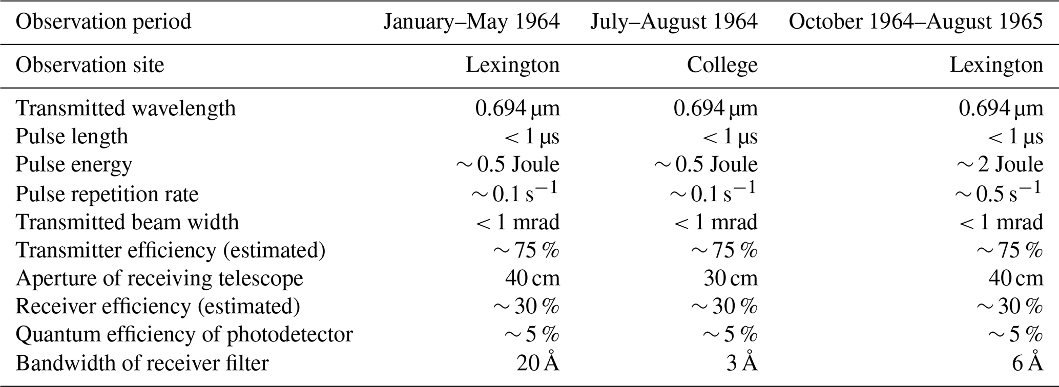
A problem with these early ruby lasers was the fluorescent emission which followed the laser pulse. These lidars incorporated a rotating shutter in the transmitting unit, synchronized with the Q-switching. The sensing unit for the backscattered signal consisted of an astronomical telescope with an interference filter and photomultiplier tube synchronized to another rotating shutter to avoid exposure to the intense returns from short distances. The photomultiplier was cooled with methanol and dry ice to reduce the dark current (Grams, 1966).
However, after initial failed searches of digital archives at several institutions, we discovered that the original lidar backscatter ratio profile measurements from the Lexington and Alaska 1964/1965 soundings are fully tabulated in Gerald W. Grams' PhD thesis conducted under the supervision of Giorgio Fiocco (Grams, 1966, hereinafter identified as G-66). Fortunately, at those times it was quite common for some observational datasets to be tabulated within PhD theses, grant reports, etc., a practice that after several decades is becoming required again, with many journals now mandating authors to make available the data they use via a recognized open-access data archive.
Dhomse et al. (2020) used preliminarily processed lidar data from Lexington, MA, one of the two sites reported in Grams and Fiocco (1967) to compare model aerosol extinction at 16 km with lidar observations, finding good agreement. Dhomse et al. (2020) and Niemeier et al. (2019) also noted the large change in the volcanic forcing for the Agung periods with the volcanic aerosol datasets used in the Coupled Model Intercomparison Projects 5 and 6 (CMIP5; Taylor et al., 2012; CMIP6; Eyring, et al., 2016; Zanchettin et al., 2016). The importance of reducing uncertainty by reconciling the datasets with additional stratospheric aerosol observations was also identified within these studies. Only an initial (preliminary) version of the Lexington 550 nm aerosol extinction dataset was used in Dhomse et al. (2020), with the analysis here producing a vertical profile dataset between 12 and 24 km. An important aspect of the dataset here is the two-way transmittance corrections applied to the aerosol backscatter ratio when deriving the aerosol extinction and optical depth datasets, with a detailed and transparent assessment of the relative error in each quantity also included.
This work is a contribution to the data rescue activity of the Stratospheric Sulfur and its Role in Climate (SSiRC), a SPARC (Stratosphere–Troposphere Processes and their role in Climate) initiative (SSiRC, 2020). The 1964/1965 lidar data recovered here follows on from another important volcanic aerosol dataset recovery of two ship-borne lidar datasets that measured the progression of the highly uncertain “tropical core” of the Pinatubo aerosol cloud from 17 July to 13 September 1991, 4–12 weeks after the 15 June 1991 Pinatubo eruption (Antuña-Marrero et al., 2020b). Those datasets were an identified priority within the SSiRC data rescue activity since they provide new constraints within the period when the Stratospheric Aerosols and Gas Experiment II (SAGE II) satellite could only observe the upper part of the Pinatubo aerosol cloud due to the saturation of the aerosol extinction retrieval (e.g. Thomason, 1992; McCormick and Veiga, 1992).
2.1 Lidar instrumentation
The first successful laser radar ranging experiment was conducted at the Research Laboratory of Electronics, Massachusetts Institute of Technology, at Lexington, Massachusetts, and consisted of analysing the return signal from a short pulse (micro-second) laser covering the 60–140 km altitude range (Smullin and Fiocco, 1962). The research team, led by Giorgio Fiocco, continued developing applications of the lidar for atmospheric research. Scattering layers were detected in the upper atmosphere between 110 and 140 km (Fiocco and Smullin, 1963) and were interpreted to originate from meteoric fragments entering the outer atmosphere (Fiocco and Colombo, 1964). After some changes and improvements, stratospheric aerosols were detected between 10 and 30 km altitude, and the first lidar measurements of the stratospheric aerosol layer began (Fiocco and Grams, 1964).
The schematic diagram and a photo of the instrument are in Figs. 3 and 4 of G-66, respectively. Also listed are the main features of the lidars used for the measurements at Lexington and College, Alaska, reproduced in Table 1. Both lidars used a Q-switched ruby laser at the 694 nm wavelength.
2.2 Lidar measurements
Lidar observations were conducted at Lexington, Massachusetts (42∘25′ N, 71∘15′ W), and at College (64∘53′ N, 148∘3′ W), located in the city of Fairbanks, Alaska, hereinafter identified as Fairbanks. The measurements were supported by the NASA Grant NGR-22-009-131. One of the semi-annual reports mentions more than 100 measurements conducted (Fiocco, 1966a). However the number of profiles appearing in Grams' PhD dissertation was 75. A total of 9 d of measurements from 26 July to 21 August 1964 were conducted at Fairbanks. At Lexington, Massachusetts, 23 d of measurements from 14 January to 20 May 1964 and 43 d from 11 October 1964 to 21 July 1965 were made. At both sites, measurements were restricted to dark nighttime conditions. A single laser shot was registered by photographing the return signal on an oscilloscope covering up to 40 km and then digitized by hand. The digitized return signals from a set of laser shots were then averaged in 1 km bins (G-66; GF-67).
2.3 Backscattering ratios in the original lidar dataset
It is well known that solving the lidar equation for the single-wavelength elastic lidar is an ill-posed problem. The return signal is the result of scatter from both molecules and aerosol particles; hence additional information is necessary to separate their contributions (e.g. Kovalev, 2015). Considering this fact, we may understand the magnitude of the challenge confronted by Giorgio Fiocco and then Gerald W. Grams, Giorgio Fiocco's PhD student, when they conducted the processing of the first ever set of lidar return signals from stratospheric aerosols.
First, we describe the procedure applied in G-66 to derive the backscattering ratio at 694 nm and range z, SR(694, z). The average photoelectron flux (electrons per second) registered by the photomultiplier, which is proportional to the backscattered signal, was represented in Eq. (3.8) of G66 as follows:
where z is the altitude, σT(z) the total radar cross-section per unit volume of atmospheric constituents at z, and K is a constant resulting from all the terms not depending on the altitude in the optical radar equation, including T2w , the two-way atmospheric transmittance (see G-66 for more details). The assumption of a constant value for T2w in the stratosphere was based on the atmospheric attenuation model proposed by Elterman (1964). The model provided magnitudes of the molecular and aerosol scattering, as well as the ozone absorption, showing that almost all attenuation of the laser beam occurs in the troposphere. The model gave an estimate of the variability in the term T2w, at 700 nm in the stratosphere, between 10 and 30 km, which was below 3 %. The correction of the return signal, associated with the two-way transmittance of the laser beam throughout the atmosphere, was then neglected, and it was assumed that the atmospheric extinction term was constant. This is a good assumption for times of low stratospheric aerosol loading. For enhanced stratospheric aerosol, e.g. after volcanic eruptions, however, aerosol extinction becomes important, reduces the stratospheric transmission, and makes it range dependent.
The return signal from a set of laser shots was averaged in time and in altitude to a resolution of 1 km between 12 and 30 km. Next, the ratios between the averaged signal at each level and the values at the same level of the right side of Eq. (1) were calculated for each profile between 12 and 30 km. A final step for each profile consisted in normalizing the ratios calculated in each profile between 12 and 24 km, with the average ratios between 25 and 30 km producing the derived SR(694, z) under the assumptions already cited. The normalization procedure assumed the contribution from aerosols was negligible above 24 km, leading to an underestimate of stratospheric aerosol since there would have been aerosol at these altitudes (Russell et al., 1979).
The SR(694, z) values derived from the lidar measurements conducted at Lexington and Fairbanks were reported in tabular format in Gerald W. Grams' PhD thesis (G-66) and cited in the acknowledgements section of GF-67. It was the unique reference of its existence that was the clue that guided us in our search for the lidar measurements.
2.4 Algorithms used in the processing
The SSiRC data rescue activity is committed, whenever it is possible, to re-calibrate each dataset and determine its levels of uncertainties (SSiRC, 2020). Because some stratospheric aerosol lidar datasets have already been identified and located, we endeavour to reprocess them using a standardized algorithm to guarantee the best possible consistency among the different lidar datasets. Below, we describe the processing algorithm as a first step in that direction.
The lidar backscattering ratio, SR(λ, z), is commonly defined as the ratio between the total backscatter βT(λ,z) and the molecular backscatter βm(λ,z) at the altitude z and wavelength λ. βT(λ,z) is the sum of βm(λ,z) and the aerosol backscatter, βa(λ,z):
βm(λ,z) is derived using the following equation:
where is the molecular extinction to backscatter ratio for the molecular scattering, commonly approximated by (Collins and Russell, 1976) after neglecting the dispersion of the refractive index and the King factor of the air represented by kbw. The volume molecular scattering coefficient, σm(λ,z), is determined by the following equation:
where (mol−1) is Avogadro's number, Ra= 8.314472 (J K−1 mol−1) is the gas constant, and Qs(λ) the total molecular scattering cross-section per molecule for the standard air. The derived equation for Qs(λ) for standard air is (Hostetler et al., 2006)
The single-wavelength elastic lidar systems provide profiles of attenuated total backscatter. The “true” total backscatter is calculated from , where . Substituting into Eq. (2), taking into account that , and re-arranging specifically for the case of the 694 nm backscattering ratio give
Whereas the term Tj(λ,z) in Eq. (6) usually specifies the full two-way transmittance correction, at this stage of the processing methodology, we correct only for the attenuation due to molecular backscatter and ozone absorption:
The αj(λ,z) term is thus the vertical profile of 694 nm extinction due only to molecules, αm(λ,z), and ozone absorption, , with zo being the altitude of the lidar. This postponement of the aerosol attenuation correction is due to the 500 nm wavelength of the contemporaneous aerosol optical depth (AOD) measurements being much closer to the target wavelength of 532 nm, the method preserving the two-way molecular and ozone transmittance corrections to be applied at the measurement wavelength of 694 nm.
The conversion to aerosol extinction is carried out after first translating the aerosol backscatter from 694 to 532 nm and then applying the corresponding wavelength exponent kb(z,t) calculated from in situ size distribution measurements of the Northern Hemisphere mid-latitude Pinatubo aerosol cloud (Jäger and Deshler, 2002, 2003):
Note again that the derived 532 nm aerosol backscatter, βa(532,z), has at this point only been corrected for two-way molecular scattering and ozone absorption transmittance effects.
The aerosol extinction, αa(532,z), at this point still uncorrected for two-way aerosol transmittance, is then calculated by the following expression:
where EBc(z,t) are altitude- and time-dependent coefficients to convert aerosol backscatter to aerosol extinction (at λ=532 nm), derived from the same Pinatubo aerosol size distribution measurements (Jäger and Deshler, 2003).
Both the EBc and kb factors are derived from log-normal size distribution fits to balloon-borne optical particle counter measurements of the Pinatubo aerosol cloud from Laramie, Wyoming, USA. Each of the conversion factors in Jäger and Deshler (2002, 2003) represent averages over four height ranges – tropopause–15, 15–20, 20–25, and 25–30 km – and are provided for the 4-month periods November–February, March–June, and July–October of each year after the eruption. We used EBc(z,t) and kb(z,t) for the same 4-month periods after the March 1963 Agung eruption, based on matching the same time offset after the Mt. Pinatubo 1991 eruption.
The algorithms for the solution of the single wavelength lidar equations apply the two-way transmittance correction to the raw lidar return signal, together with squared distance correction, before the backscattering ratio is calculated. In our case the only measurement information we have is the lidar backscatter ratios, which have been derived without conducting the two-way transmittance correction (G-66) for any species. However, only the molecular and ozone two-way transmittance corrections, Tm(694,z) and , were included in Eq (6) by the reasons explained below.
As explained above, the aerosol two-way transmittance correction, Ta(532,z) , was deliberately postponed until the final step to derive due to the available contemporaneous measurement information for AOD being at λ=500 nm (see Supplement). We converted the measured AOD at 500 to 532 nm using Ångstrom exponents covering the cited wavelength range from 1995 to 2019 from the nearest Aerosol Robotic Network (AERONET, 2020) stations. Although the tropospheric aerosol layer in the eastern USA will have had different physical and chemical properties in the 1960s (e.g. Went, 1960; Husar et al., 1991), this is only a small change in wavelength, with the method then introducing much less error than had we converted from 500 to 694 nm to apply the aerosol attenuation correction. We note that the calculated monthly mean total AOD (TAOD) at 532 nm from Blue Hill Observatory, MA, from 1961 to 1966 is in the range from 0.1 to 0.4, consistent with the elevated background TAOD reported for the eastern USA during the 1960s (Husar et al., 1981; Sect. S1 in the Supplement).
We produced a first guess for each measurement day at each site in the range from 11 to 24 km. The , a unique value from the lidar altitude to 11 km, was calculated using Eq. (7) and the TAOD value for the month in which the measurement was conducted. values from 12 to 24 km were calculated using Eq. (7) and the uncorrected αa(532,z).
The first guess aerosol scattering corrected by the total two-way transmittance, , was derived by applying the correction for the two-way aerosol transmittance Ta(532,z):
Since we are using the measured TAOD, which included the stratospheric AOD, to calculate the first guess , we applied a second step after producing a first guess profile, for which we then calculate the stratospheric AOD (sAOD*), integrating between 12 and 24 km. Then sAOD* is used in Eq. (11) to estimate the tropospheric AOD (tAOD) for each measurement:
The former values for each measurement will be replaced by new ones derived using the calculated tAOD corresponding to each measurement. Then the final profile of Ta(532,z) for each measurement will consist of the new Ta(532,11 km) calculated using tAOD and the already derived Ta(532,z) values from 12 to 24 km that were calculated using the uncorrected αa(532,z) in Eq. (7). Those profiles of Ta(532,z) are applied in Eq. (10) producing the definitive values of .
The method we applied uses monthly means of the TAOD from the sun photometer, converted from 500 to 532 nm (described above), assuming this to be tropospheric (tAOD) in the first step, to produce for each site a profile so as to account for the tropospheric aerosol transmittance from the lidar altitude across the troposphere up to 11 km and the stratospheric aerosol transmittance in the lower stratosphere from 12 to 24 km. However, when the stratospheric AOD (sAOD*) is calculated in the next step (from the first guess ), the resulting first guess total AOD (tAOD + sAOD*) will be higher than the observed TAOD. The second step is aimed at estimating the magnitude of a consistent value of tAOD for each measurement to constrain tAOD + sAOD ≤ TAOD.
Although more iterations of those final steps would be possible, with the high magnitude of the estimated mean error, around 60 %, compared to an estimated 15 %–20 % maximum improvement achieved by the iteration procedure, we do not believe those additional calculations would be worthwhile in this case.
2.5 Complementary datasets used
The correction for the attenuation of the lidar signal by the two-way transmission by atmospheric molecules, ozone, and aerosols is often considered negligible and ignored based on signal to noise ratio considerations or for simplicity (e.g. G-66; GF-67). We were motivated to make that correction by the fact that the accuracies of the different instruments available for measurements of the stratospheric aerosols from the 1963 Mt. Agung eruption are still under scrutiny and discussion (e.g. Deirmendjian, 1965, 1971; Dyer, 1971a, b; Clemesha, 1971; Stothers, 2001; Timreck et al., 2018). Our goal was to produce the consistently processed aerosol extinction and optical depth from the rescued measurements based on the contemporary state of the art measurements in the 1960s. For the different data sources and processing algorithms, we calculate the two-way transmittance corrections by atmospheric molecules, ozone, and aerosols as described in Sect. S1.
2.6 Numerical and statistical methods
For each of the two datasets we calculate percentage differences (Δα*US) between αa(532,z)US calculated using the same βm(694,z) profile from the 1962 US Standard Atmosphere for all the days and the calculated using the βm(694,z) profiles derived from the daily soundings,
and the percent differences by the following expression:
Similarly we defined the differences, Δαat2w, and the percent differences, Δαat2w %, between the calculated using the βm(694,z) profiles derived from the daily soundings and its corrected values, αa(532,z)t2w, resulting from accounting for the two-way atmospheric transmittance.
Also, for cumulative aerosol optical depth in the 12 to 24 km layer, we define and τa(532,z)US calculated from the and αa(532,z)US, respectively, as
and the percent differences, , by the following expression:
2.7 Relative error estimates
The present evaluation of the relative errors in the different processing steps of the single wavelength elastic lidar followed the algorithms developed by Russell (1979). Whenever it was possible, we calculated the different terms of the equation based on the available dataset error. In several cases we combined information from the rescued metadata associated with the measurements and from available additional information in the literature.
2.7.1 Backscattering ratio relative error
We use Eq. (19) from Russell (1979) quantifying the contributions from the different sources to the relative error in backscattering ratio :
where SR(λ,z) is the total backscattering ratio; Ns is the signal measured; TT is the two-way transmittance from aerosols, molecules, and ozone; βm is the molecular backscattering; is molecular backscatter at the normalization level; SRmin(λ,z) is total backscattering ratio at the normalization level; and is the covariance between measured βm and .
For estimating the magnitude of the signal measurement error we rely on the information provided by G-66. He estimated statistical fluctuation of the signal, the shot noise of the photodetector, and other sources of the order of 0.2 % to 3 %. For both Lexington and Fairbanks we assume %.
As cited above, according to G-66 if no TT correction was conducted, then the term .
Because in the calculation of SR(λ,z), values of Nd(z) from the 1962 US Standard Atmosphere were used (G-66), it was assumed % for both sites (e.g. Russell et al., 1979). In addition we assumed and after assuming measurement errors are uncorrelated. The use at the lidar levels of interpolated βm values from the lower-resolution ones calculated using the US 1962 Standard Atmosphere support the former assumption.
The term δSRmin was calculated according to Table (1b) in Russell (1979) for SRmin=1.01 and the respective latitudes of both sites. Then following Russell et al. (1979), we assume
2.7.2 Aerosol backscattering relative errors
Equation (18) in Russell (1979), estimating the relative error in βa(694,z), can be approximated in our case by
The estimated error for the two-way transmission corrections in Russell et al. (1979) provides the following expression,
and considering the standard error of determination of τa, , and τm being respectively 50 %, 20 %, and 10 %, the following estimates are produced: δτa=0.5τa, , and δτm=0.1τm . However, in our calculation of βa, only the ozone and molecular two-way transmittances were used.
For this section of the procedure, we consider %. We neglected the error in computing Qs using Eq. (5) because its maximum relative error is 0.2 % for a spectral region of 350–1600 nm (Hostetler et al., 2006), well below the errors in .
Next, we determined the relative error in βa(532,z) associated with the conversion from βa(694,z) in Eq. (7) using the wavelength exponents, kb(z,t), for aerosol backscatter in the range of wavelengths between 694 and 532 nm (Jäger and Deshler, 2003). The errors were estimated from their Fig. 1 with %:
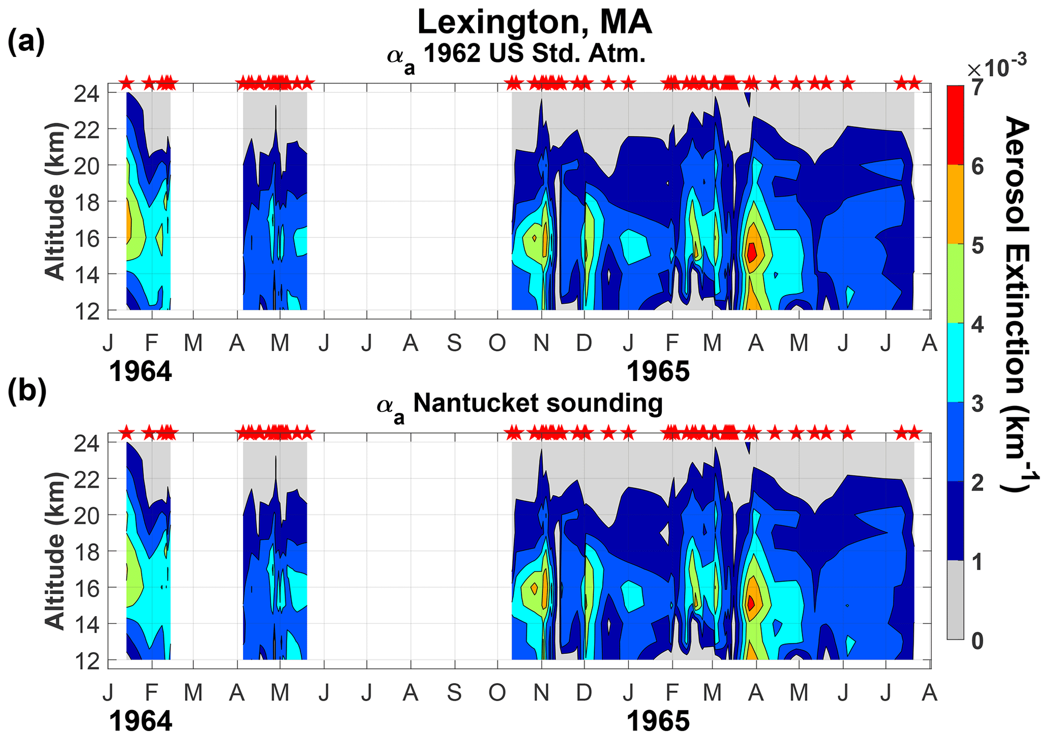
Figure 1(a) Contour plot of the vertical profiles of 532 nm aerosol extinction αa(532,z) calculated using the same βm(694,z) profile from the 1962 US Standard Atmosphere for all the days. (b) The contour plot of the vertical profiles of 532 nm aerosol extinction αa(532,z) was calculated using the daily βm(694,z) profiles from the sounding at Nantucket, MA. The red stars indicate the dates the measurements were conducted. The measurement gaps longer than 1 month – March, and July to September both in 1964 – have been left blank.
Table 2Relative differences between the and , as well as and .

2.7.3 Aerosol extinction relative errors
In the case of the αa, its relative errors are
The last term in the right side represents the error in the EBc for λ=532 nm. In the case of the ones we used (Jäger and Deshler, 2002, 2003) the error has been estimated at ±40 % according to Deshler et al. (2003). For , the aerosol extinction corrected by the aerosols' two-way transmittance using the estimates of its relative error described above is
Using the cited set of equations and the assumptions described above we evaluated the error for each altitude in each measurement.
3.1 The 532 nm aerosol extinction profiles and optical depth
In Fig. 1 we show contour plot of the vertical profiles of 532 nm aerosol extinction, αa(532,z), for Lexington calculated using the same βm(694,z) profile from the 1962 US Standard Atmosphere for all the days and the daily βm(694,z) profiles derived from the sounding at Nantucket, MA. If measurement gaps are longer than 1 month (March 1964, and July to September 1964), they have been left blank. The temporal and vertical contour plots of the aerosol extinctions were generated using a linear time interpolation.
In general, the contour plots show a high level of variability in the aerosol extinction for Lexington both in time and altitude associated with the complex thermodynamic processes in the upper troposphere–lower stratosphere. Three main maximums are identified across the entire period. The first is between 16 and 18 km at the beginning of the record in mid-January 1964, the second between 14 and 16 km by November 1964, and the third at the same altitude but in the transition between March and April 1965. Evident is the decaying altitude of the maximums in time typical of the volcanic aerosol clouds in the lower stratosphere. However, the occurrence of the absolute maximum at this time cannot be attributed to the volcanic aerosols from Mt. Agung, as will be discussed below. No long-term analysis of this type could be conducted in Fig. 2 for Fairbanks because of the very short period of time it covers. However, the cross-section of for Fairbanks reveals maximum values between 14 and 16 km, with the absolute maximum around mid-August centred at 15 km. The magnitudes of are slightly higher than the ones from for both sites, and it is also true for and . This is quantified in Table 2. The magnitude of the mean percent difference increase in both variables is around 1 %.
This difference disagrees with G-66 in that he found retrievals using the 1962 US Standard Atmosphere slightly lower than the more realistic ones using soundings, but the differences are within calculated errors. He arrived at that conclusion from “a cursory examination” of the local variations of molecular number density, Nd(z), estimated with the Temp(z) profiles from ozone soundings at Bedford, MA (Hering and Borden, 1967). He reported Nd(z) variability rarely exceeded 5 % of the NdUS(z) values at altitudes between 10 and 30 km.
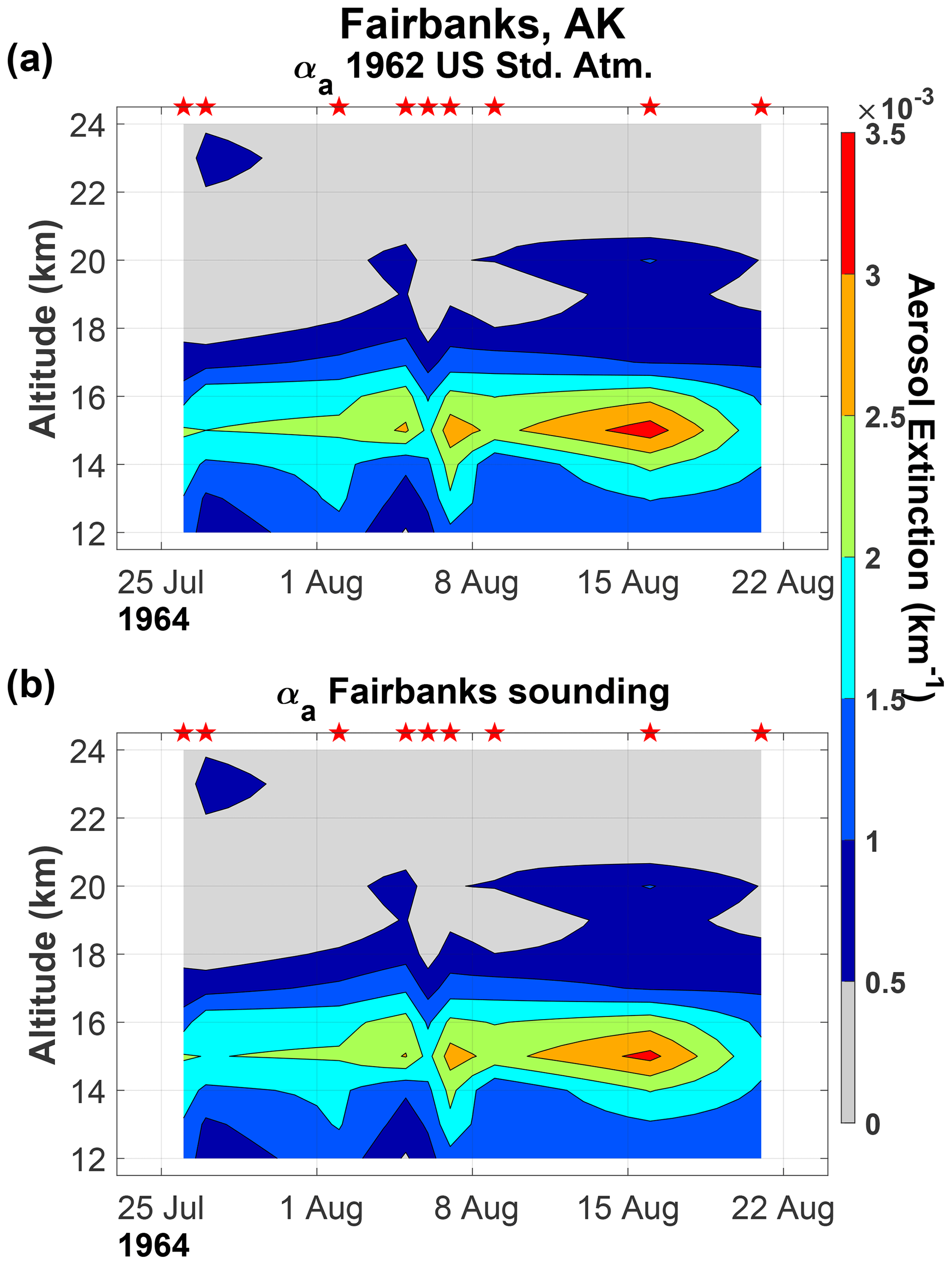

Figure 3Differences between the number molecular density, Nd(z), from soundings and from the 1962 US Standard Atmosphere in the region from 12 to 24 km. Panel (a) represents Nd(z) from Nantucket soundings used for Lexington and (b) Nd(z) from Fairbanks.
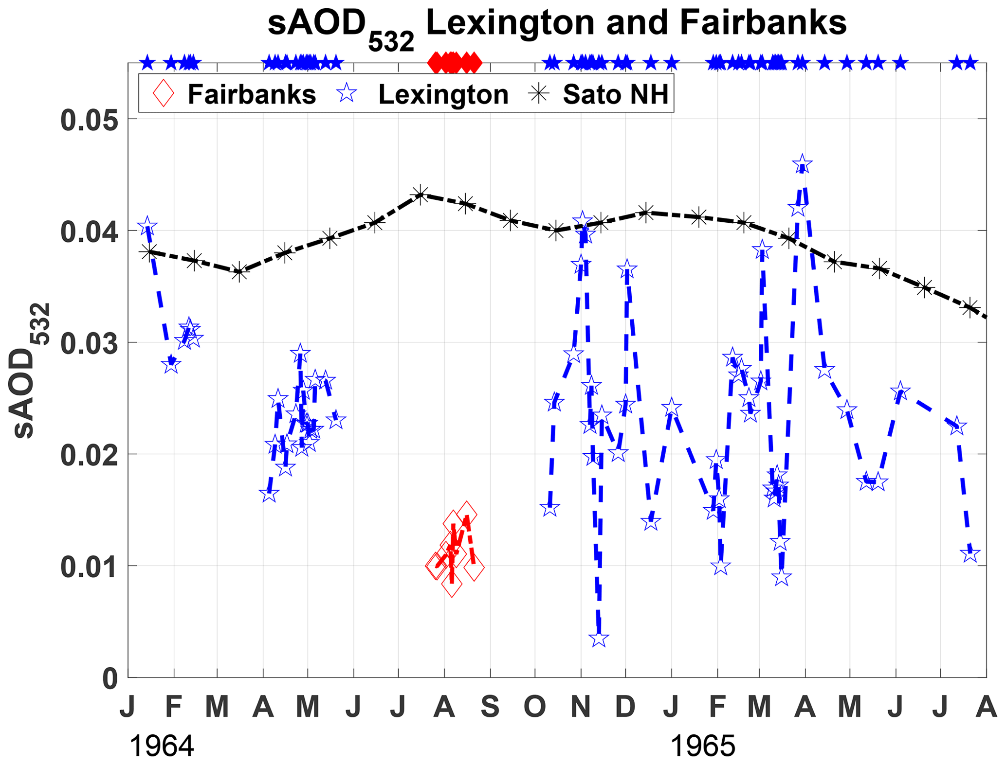
Figure 4Stratospheric aerosol optical depth (sAOD532) for Lexington (blue stars), Fairbanks (red diamonds), and for the Northern Hemisphere (black asterisks) for the period in which the measurements were conducted. The sAOD532 values were calculated from the derived using local soundings. Blue stars and red diamonds on the top axis of the figure are the dates on which the measurements were conducted.
To estimate the effects of the differences between the magnitudes of NdUS(z) and Nd(z) in the backscattering ratios, we calculate the differences between the ratios defined by
MdUS and Md are the mean values of NdUS(z) and Nd(z) between 25 and 30 km, replicating the procedure used by G-66. In Fig. 3 the differences ΔNd(z) for 66 soundings at Nantucket and the 9 for Fairbanks are plotted. For Lexington, ΔNd(z) values are both negative and positive, but higher values of NdUS(z) dominate. For Fairbanks NdUS(z) always is greater.
The errors in lidar retrievals of , attributed to the use of Temp(z) and Pr(z) from a model atmosphere to retrieve Nd(z), are of the order of 3 % and decrease to 1 % when the source of Temp(z) and Pr(z) are soundings (Russell et al., 1979). Again in Table 2, the magnitudes of the absolute differences between the US 1962 Standard Atmosphere and the soundings at Lexington and Fairbanks for αa(532,z) are of the order of 3 %, agreeing with the error attributed if case models are used instead of soundings to derive βm(λ,z).
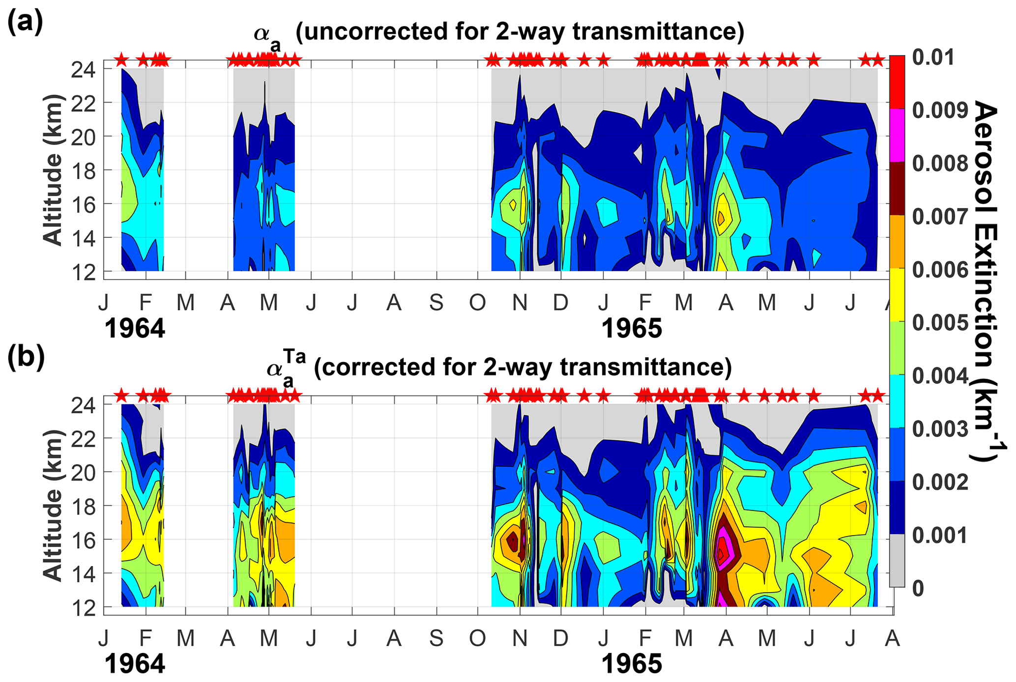
Figure 5Contour plots of the vertical profiles of 532 nm aerosol extinction at Lexington, showing values uncorrected and corrected for two-way transmittance, . The red stars indicate the dates on which the measurements were conducted.
Figure 4 shows both for Lexington (blue stars) and for Fairbanks (red diamonds). The means for the entire period of measurements available at each site are 0.0215 and 0.0099, respectively. Also shown is a monthly mean τa for the Northern Hemisphere (Sato et al., 1993). The mean at Fairbanks is half that at Lexington, providing evidence of the decreasing aerosol amount with increasing latitude. Because of the variability in , values from Lexington vary widely from the Fairbanks mean to the Sato et al. (1993) magnitude, the current reference for this period. However, as we will see in the next section, better agreement is found when the measurements are corrected with two-way transmittance attenuation.
Taking into account the small difference between the results using the US 1962 Standard Atmosphere and the soundings to derive βm(λ,z), the first simpler option can reliably be used. However, we decided to use the soundings to minimize the errors and to capture the more realistic features of the aerosol cloud.
Table 3The same as Table 2 but for the comparison of vs. and vs. . See text for details.
3.2 Aerosols extinction contour plots and optical depth corrected by aerosol two-way transmittance attenuation
Figure 5 shows the contour plots of for uncorrected and corrected two-way transmittance, , for Lexington. The initial values of TAOD were used to obtain a first estimate of . This is only used to calculate sAOD for each day and is subtracted from TAOD to produce the tropospheric-corrected value (tAOD); the calculation is repeated to determine new profiles of the two-way aerosol transmittance and correct generating . Panel (a) shows the contour plot of uncorrected values of and panel (b) the contour plot of . The magnitudes of are higher than . The two-way transmittance correction is dominated by the aerosols, in particular the tropospheric aerosols. The maximum extinction is at the third maximum, 1.071 km−1 located at 15 km, on 27 March 1965. Similarly in Fig. 6, the Fairbanks contour plots for and show a notable difference in magnitude. Here the absolute maximum extinction occurred on 16 August 1964 at 15 km with a magnitude of 3.8 km−1.
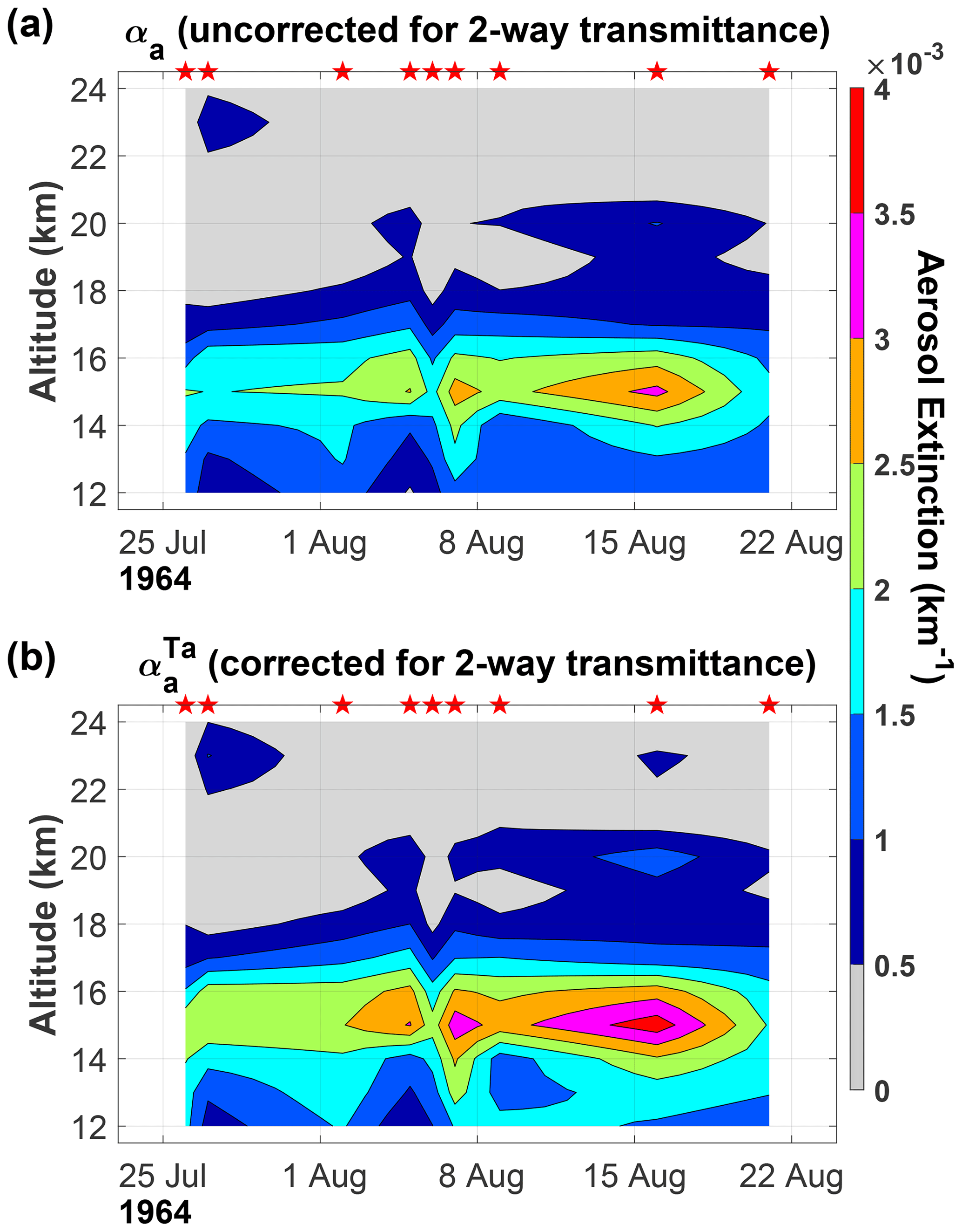
Figure 6Contour plots of the vertical profiles of 532 nm aerosol extinction, , at Fairbanks, showing values uncorrected and corrected for two-way transmittance, . The red stars indicate the dates on which the measurements were conducted.
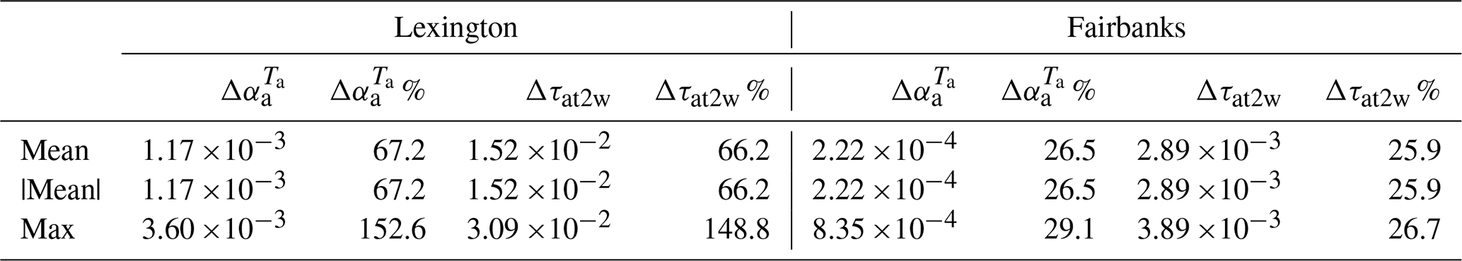
Table 3 contains the relative and absolute means and maximums for , , , and calculated using Eqs. (14) to (17) respectively but for vs. and vs. . The magnitude of produced by the two-way transmittance correction is of the order of 10−3 km−1 for Lexington and 10−4 km−1 for Fairbanks or an increase of 67 % and 26 %, respectively. These increases are due mainly to the two-way aerosol transmittances dominated by the tropospheric AOD with magnitudes more than twice as high at Lexington than at Fairbanks. The increase in magnitude reveals more details of the vertical distribution of the and in the case of Lexington the presence of a fourth maximum during May 1964 whose vertical location matches the decreasing trend at the core of the stratospheric aerosol cloud.
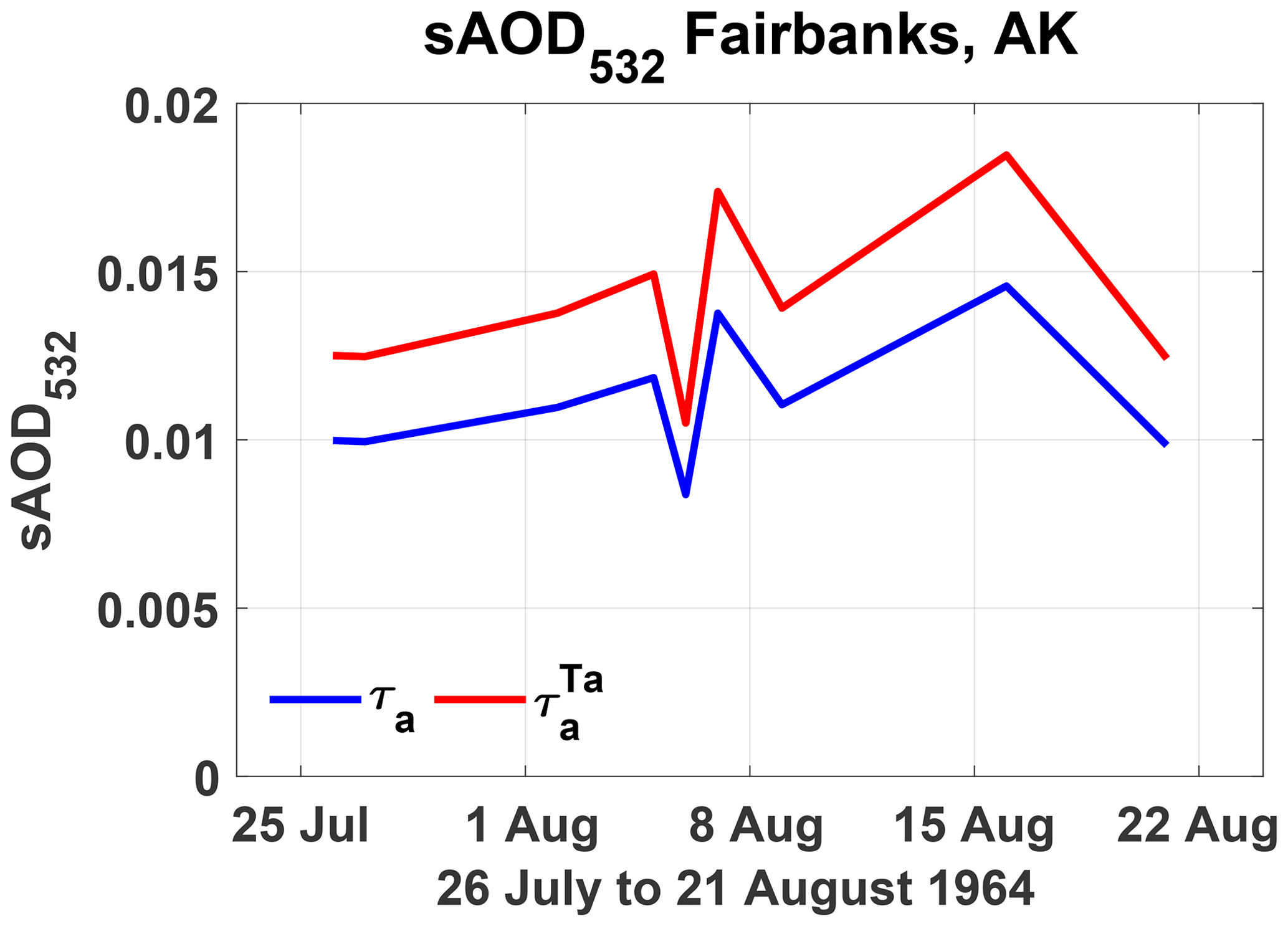
In Figs. 7 and 8 the increases in with respect to for Fairbanks and Lexington are shown. At Lexington the magnitudes are approximately the values of τa from Sato et al. (1993) for the Northern Hemisphere (black line). This agreement is an important confirmation of the Sato et al. (1993) magnitudes for τa from Agung in the Northern Hemisphere. Again in Table 3, the magnitudes of the increase in are of the order of 10−2 for Lexington and 10−3 for Fairbanks, representing 66 % and 26 % increases, respectively.
At Lexington the absolute maximum value of , 0.071, occurs on 30 March 1965, 3 d after the absolute maximum extinction was registered at 15 km. At Fairbanks the absolute maximum value of , 0.018, was registered on 16 August 1964, the same day the absolute maximum extinction was registered at 15 km at this site.
Since the pioneering lidar work by Fiocco and Grams (1964), multiple researchers have contributed to the development of the processing algorithms to retrieve aerosol optical properties and errors (Russell et al., 1979; Klett, 1981, 1985; Kovalev, 2015). These works explain the limitations of retrieving the full set of optical variables characterizing the stratospheric aerosols from the dataset of Fiocco and Grams (1964). However, assuming a Junge size-distribution model and Mie scattering with a refractive index of 1.5, Fiocco and Grams did produce estimates of the aerosol content of the stratosphere at 16 km: number concentration, surface area, and the aerosol density per unit volume of air. They also used the mean profile they derived to estimate the total particles per cubic centimetre, total surface area, and a total mass, integrating the concentrations obtained between 12 and 24 km (GF-67). The only available optical property estimates, based on some of the cited particle concentration estimates at 16 km and in the column, are the aerosol extinction at 16 km ( km−1) and the aerosol optical depth (0.015), both at 694 nm (Deirmejian, 1971).
For comparing with the values reported above, we estimate αa(694,z) from αa(532,z), as well as τa(694,z) from τa(532,z), using the wavelength exponents for aerosols from Mt. Pinatubo in the range of wavelengths from 532 to 694 nm (Jäger and Deshler, 2002). We made the estimates for both Lexington and Fairbanks as no clear assignation of the values to either site is made in G-66 or GF-67. At 16 km, the mean value of αa(694,z) was 10−3 km−1 for Fairbanks and km−1 for Lexington, matching the order of magnitude estimated by Deirmejian (1971).
From 1963 to mid-1965, in addition to the 1963 Mt. Agung eruption, two other volcanoes were reported to have erupted in the Northern Hemisphere with Volcanic Explosivity Index (VEI) 3. They were Trident Volcano in Alaska at 58∘ N and 155∘ W and the Vestmannaeyjar volcano (also known as Surtsey) south of Iceland at around 63∘ N and 20∘ W. The first was reported to have erupted in April 1963, and its plume reached 15 km (Decker, 1967). The second remained in eruption between November 1963 and February 1964, with its plume in November 1963 reaching an altitude around 4.5 km above the tropopause more than once, located approximately at 10.5 km (Thorairinsson, 1965). They were attributed as contributing to the replenishment of aerosols in the mid-latitude lower stratosphere, following the increase in the atmospheric turbidity determined using twilight measurements (Cronin, 1971).
Twilight measurements revealed three peaks in atmospheric turbidity between the March 1963 Agung eruption and the end of 1965 shown in Fig. 1 from Volz (1970). The first turbidity peak in that figure with the highest magnitude was registered by the end of 1963, when no lidar measurements were available, but its decaying is seen in the sAOD during the first half of 1964 in our Fig. 4. The second turbidity peak, having approximately the same magnitude as the third, is located in the last months of 1964, coincident with the second sAOD peak in Fig. 4. The third turbidity peak also coincides with the third sAOD peak. Updated information reveals the extension in time of the Vestmannaeyjar, from late 1963 to the middle of 1964 (GVP, 2013a), and the occurrence of two additional eruptions of Trident Volcano, the first between 17 October and 17 November 1963 and the second on 31 May 1964 (GVP, 2013b), all of them at VEI 3. That sustained input of the aerosols in the Northern Hemisphere stratosphere explains the second and third peaks with similar magnitudes in the turbidity (Fig. 1 in Volz, 1970, and in the sAOD in our Fig. 4).
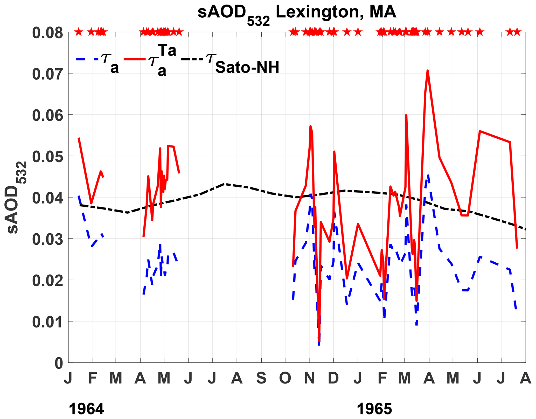
Figure 8Time series of stratospheric AOD (sAOD532) for Lexington for τa(532,z) and compared to that from the NASA Goddard Institute for Space Studies volcanic aerosol dataset (Sato et al., 1993).
3.3 Relative errors
Table 4 reports the results for the estimated relative errors in the aerosol extinction with and without the aerosol two-way transmittance correction for both sites. In addition, the relative errors of the backscattering ratio and aerosol backscatter at 694 nm and the aerosol backscatter at 532 nm are reported. The relative errors for km−1 were excluded in the statistics.
Note the increases in the mean relative errors from to , 12 % to 48 % at Fairbanks and 13 % to 36 % at Lexington, the higher increases occurring during the full processing. It is explained by the factor in Eq. (18). Because the processing algorithm relies on Eq. (6) to derive βa from βm, the squared ratio will be lower than 1 if SR< 2, increasing as SR decreases and reaching the value for Only with SR≥2 is the ratio lower than 1, which in the case of Fairbanks happens at one level on 1 d. In the case of Lexington, 10 % of the SR values are higher than 2.
Table 4Relative error estimates of the backscattering ratio, aerosol backscatter at 694 nm and 532 nm, and aerosol extinction with and without correction for aerosol two-way transmittance at 532 nm for Lexington and Fairbanks. Errors for km−1 were not included in the statistics. All errors are percentages.
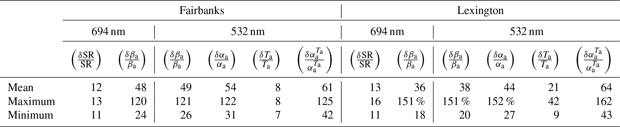
In Table 4, the second highest increase in the mean relative error occurs in the calculation of from . At Fairbanks the increase is 7 %, from 54 % to 61 %, and at Lexington the increase is 20 %, from 44 % to 64 %. The error is associated with the magnitudes of the relative errors from , conducted at this step for the reasons explained above. At Fairbanks the mean value of is 8 %, while it is 44 % at Lexington, associated with the expression δτa=0.5τa. It should be taken into account that the total AOD at both sites is dominated by the magnitude of the tropospheric AOD, which is higher at Lexington.

Figure 9(a) Contour plot of relative error estimates for Lexington. (b) Contour plot of the aerosol extinction at 532 nm corrected by two-way transmittance for Lexington . Note the two data gap periods greater than 1 month for the consecutive measurements: March, and July to September both in 1964. They are identified with vertical dotted red lines at the 7th and 23rd measurements. In the top panel the areas in white in the relative error contour plot represent relative errors for km−1. They were not included in the statistics in Table 4.
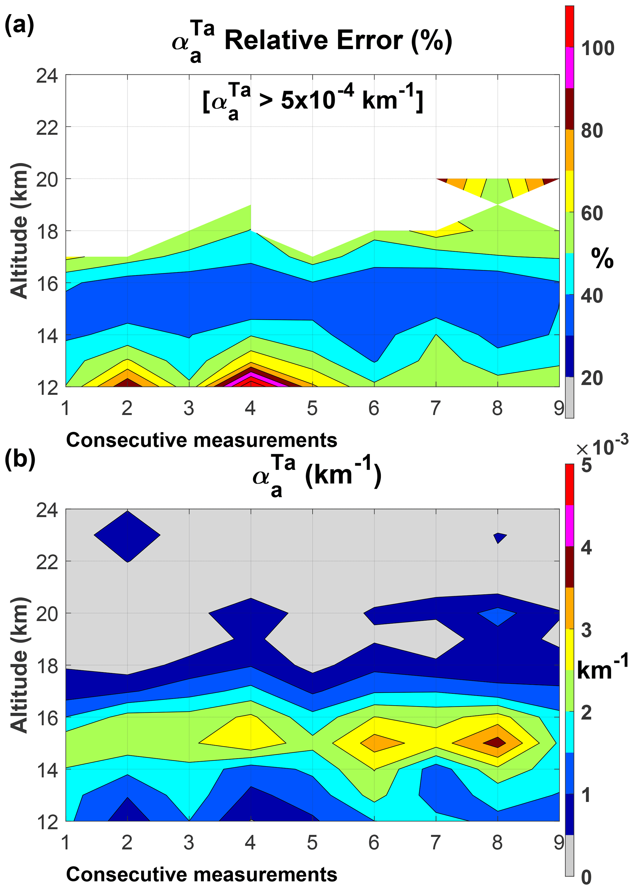
The time vs. altitude contour plots of the relative errors and of the are shown in Figs. 9 and 10 for Lexington and Fairbanks, respectively. The regions with maximum magnitudes of at both sites are associated with the lower relative errors as expected. At Lexington, for km−1 the relative errors are ≤ 30 %. It is also evident that relative errors equal to or lower than 50 % dominate both in time and altitude. In the case of Fairbanks, for km−1 the relative errors are ≤ 40 %. The relative errors of , in Table 4, produce relative errors above 100 %. Those estimated values of the relative errors for , together with the ones in Table 4, are substantially larger than other sets of volcanically perturbed stratospheric aerosols lidar measurements.
The high error magnitudes in the at 694 nm estimation could be reduced in the case that SR values increase. In several of the 75 SR profiles a renormalisation processing could increase SR magnitude. This is reasonable since the normalization altitude range (no aerosol present) was 25 to 30 km, where there certainly would be some aerosol present. An inspection of the plots of SR vs. altitude in Figs. 14, 15, and 16 in G-66 shows the presence of aerosols between 25 and 30 km. Furthermore, in some of the profiles SR is above 1 at all levels (1.0 indicates no aerosol). In addition, the introduction of the two-way transmittance correction in the processing of SR will increase SR from the raw returned lidar signal.
Options are available to find the raw lidar data to conduct the reprocessing described above. These include searching for the filmed images of the oscilloscopes used as registers and/or the original punch cards (probably transferred to tapes) both reported in G-66. A last resort would be the digitalization of the SR from the figures cited above. The original signal profiles could then be reconstructed by inverting the normalization procedure applied to produce the SR profiles.
3.4 Attribution of the 1963 Agung aerosol cloud within the Lexington lidar dataset
In this section, we seek to understand whether some of the sAOD variations observed by the Lexington lidar may originate from sources other than the March 1963 Agung eruption (such as the two stratosphere-injecting 1963 VEI 3 eruptions discussed in Sect. 3.2: Trident, Alaska, and Vestmannaeyjar, Iceland). Specifically, we compare the Lexington extinction dataset to four different model-based volcanic forcing datasets for the Agung aerosol cloud. Three of the four Agung forcing datasets are from two different interactive stratospheric aerosol models: two different SO2 emissions scenarios from the UM-UKCA model (Dhomse et al., 2020, 2021) and a third simulation from the 2D-AER model (Arfeuille et al., 2014), as applied within the CMIP6 volcanic aerosol dataset (Luo et al., 2016). The fourth simulation is from an idealized model representation of the Agung cloud, based on a simple parameterization for the progression of the tropical reservoir of volcanic aerosol, and its dispersion to mid-latitudes (Ammann et al., 2003), used to represent historical volcanic forcings in some CMIP5 climate model historical integrations (see Driscoll et al., 2012).
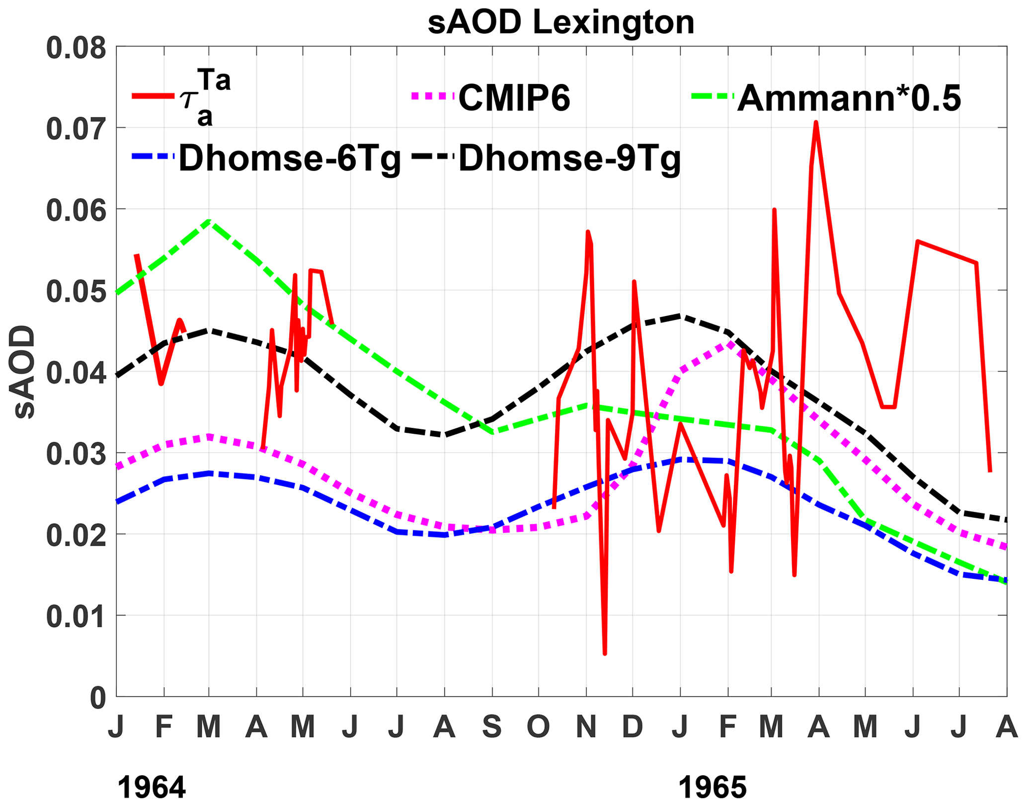
Figure 11Interactive stratospheric aerosol model (Dhomse et al., 2020) representations of the Agung aerosol cloud sAOD550 compared with that of the Lexington dataset, the Ammann et al. (2003) volcanic forcing dataset, and the CMIP6-AER2D volcanic aerosol dataset (Luo, 2016).
The progression of volcanic aerosol clouds from major tropical eruptions reaching the stratosphere was established by Dyer et al. (1970, 1974). They synthesized the extensive set of observations on the Agung aerosol cloud (Dyer and Hicks, 1968) and used the analyses of the global dispersion of radionuclides from Pacific thermonuclear tests in the 1950s (e.g. Machta and List, 1959). The continual slow upwelling circulation in the tropics and the sub-tropical barrier at the edge of the tropical pipe combine to cause the long-lived tropical stratospheric reservoir (Dyer, 1974; Grant et al., 1996), which is the reason why tropical eruptions have such prolonged radiative cooling compared to mid-latitude eruptions. The Brewer–Dobson circulation (Brewer, 1949; Dobson, 1956) has a strong seasonal cycle, transporting air preferentially towards the winter pole, causing an increasing mid-latitude sAOD trend during autumn and a decreasing mid-latitude sAOD trend during spring (in both hemispheres). Each of the model lines in Fig. 11 shows this circulation-driven seasonal variation in sAOD, with the transport of the Agung aerosol remaining in the tropical reservoir predicted to increase during October and November, reaching a peak in January to March in both 1964 and 1965. The model-predicted variations are consistent with the initial observed sAOD values of 0.04–0.05 in January and February 1964 being higher than most of the 0.01–0.04 sAOD values observed in October and November 1964, and the expected variations from the models suggest the suddenly higher sAOD values ∼ 0.05 may be from a different source than Agung. However, whereas sAOD values would be expected to increase going into winter, the December, January, and February sAOD at Lexington are mostly lower than during the autumn, which indicates an additional source of stratospheric aerosol may have continued to add to the Agung cloud sAOD throughout the autumn of 1964. Furthermore, the 1965 Lexington observations show a continuing increase in sAOD into the springtime, whereas the models predict the sAOD from Agung would have reduced by a factor of 2 during the first 6 months of 1965. The analysis suggests that another source of sAOD influential during this period (either the two VEI 3 volcanic eruptions in 1963/1964 or some other source of material into the stratosphere) must have caused the observed increase in stratospheric AOD during 1965 with a potentially substantial influence also during autumn 1964.
Figure 12 compares the vertical structure of the 9 Tg representation of the Agung aerosol cloud from Dhomse et al. (2020) at 42∘ N, compared to the Lexington observations, confirming that these model simulations capture the altitude of the cloud during the early period of the measurements (January to May 1964). However, although the magnitude of the simulated aerosol extinction compared well with the original Lexington dataset (Dhomse et al., 2020), with the two-way transmittance corrections applied here, the 9 Tg simulation is low-biased compared to the lidar measurements, even in this earlier period, suggesting the 12 Tg UM-UKCA aerosol simulation (not shown) would likely compare better (Dhomse et al., 2020, 2021). None of the four model-generated Agung forcing datasets can explain the observed increase in extinction during January to July 1965. The sudden peaks in April and June 1965 have quite a different vertical structure compared to the early 1964 measurements, the sAOD in 1965 having a substantial component from the altitude range 18–20 km. This vertical profile analysis again suggests the episodic sAOD enhancements in spring 1965 were from a different source than the 1964 measurements.
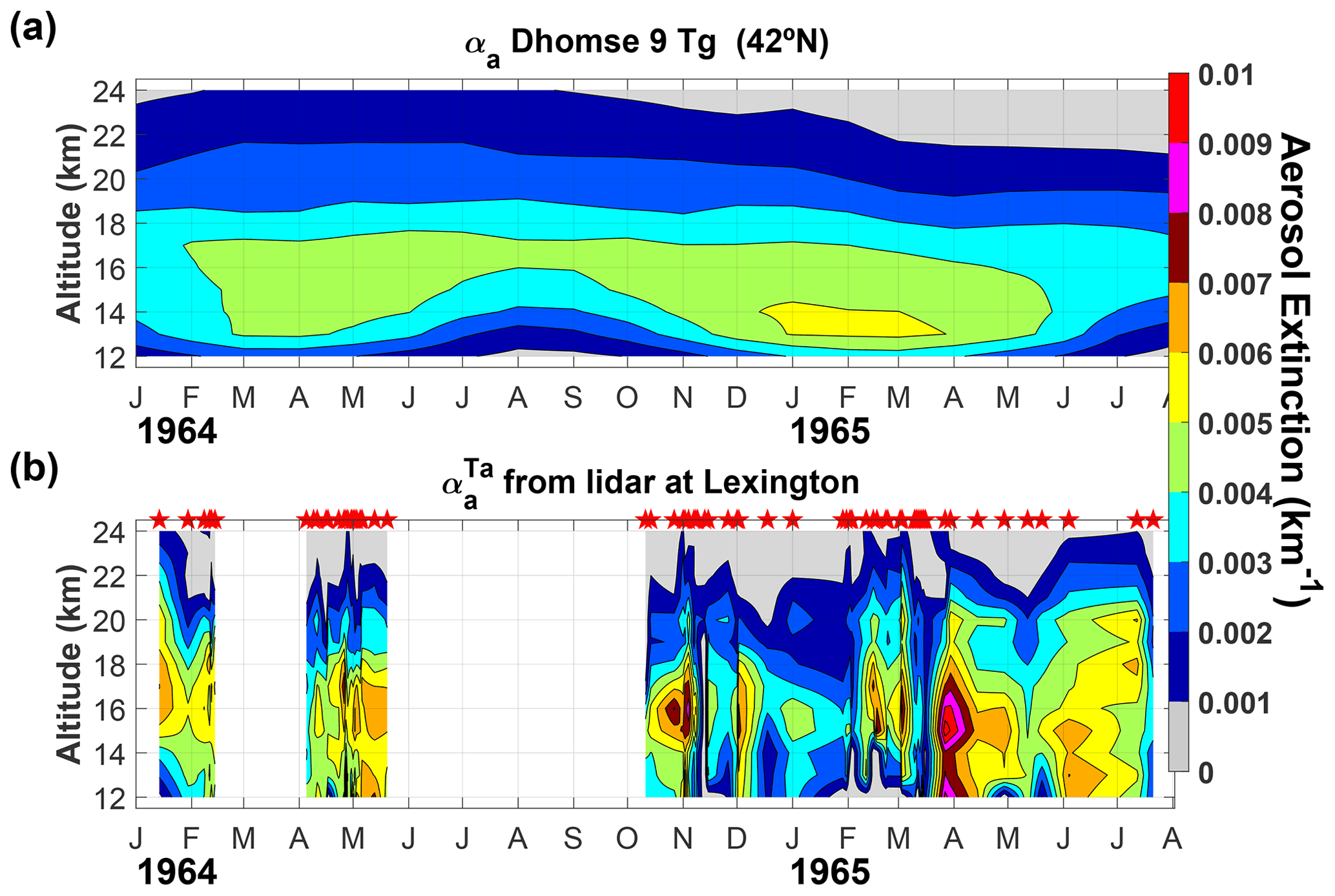
Figure 12Contour plots of from Dhomse et al. (2020) at 42∘ N and measured aerosol extinction corrected for two-way transmittance from lidar for Lexington.
The datasets of the original rescued backscattering ratios and the calculated aerosol backscatter (both at 694 and 532 nm) and the aerosol extinction at 532 nm (both corrected and uncorrected for two-way aerosol transmittances) at Lexington and Alaska are available at https://doi.org/10.1594/PANGAEA.922105 (Antuña-Marrero et al., 2020a).
We have carried out a data recovery of the first ever multi-year lidar dataset of the stratospheric aerosol layer, the Lexington and Fairbanks measurements profiling the portion of the Agung volcanic aerosol cloud that dispersed to Northern Hemisphere mid-latitudes and high latitudes, respectively. The results show the high level of variability in the stratospheric aerosol extinction for Lexington between January 1964 and July 1965 that is mainly attributed to the 1963 Mt. Agung eruption. At Lexington the highest aerosol extinction values and aerosol optical depths (1.1 km−1 and 0.076, respectively) were actually observed at the end of March 1965 in the final phase of the 1.5-year-long record. Based on contemporary and updated reports of additional volcanic eruptions in the Northern Hemisphere between 1963 and 1965, we tentatively suggest a potential explanation for the apparently contradictory temporal sAOD trends to be the VEI 3 eruptions of Vestmannaeyjar, Iceland, and Trident, Alaska. Further research combining observational data and modelling should be conducted to elucidate the individual contributions from each of those eruptions to the stratospheric aerosol layer at this location of the Northern Hemisphere.
The level of the relative errors are unusually high considering that under high loads of volcanic aerosols in the stratosphere, the signal to noise ratio is high in the returned lidar signal. The analysis of the contributions of the variables along the different steps of the processing algorithm identified the two main sources of error. The main one, accounting for a little more than 30 % of the relative error, is associated with the division of the molecular backscatter by the aerosol backscatter, which is directly linked to low magnitudes of the backscattering ratio. Those low magnitudes are produced by two factors: the first is the lack of two-way transmittance corrections in the backscattering ratio calculation from the raw squared distance-corrected signal, and the second is that the normalization altitudes, considered to be empty of aerosols, were too low and actually did contain aerosol. We suggested alternatives to search for the original signal profile records or to reconstruct the original signal profiles from the plotted backscattering ratio records, including the normalization region from 25 to 30 km. A future search for original records should also take into account the 34 missing files from the 100 referred to by Fiocco for Lexington (Waymouth et al., 1966).
In general the results reported should be considered as the first estimates. We report the comparison of the aerosol extinction values and aerosol optical depths that we calculated with information available up to the present, showing reasonable results. Improvements in the two factors cited above lead to an increase in magnitude of the aerosol extinction and optical depth in several of the profiles.
We have also compared the Lexington sAOD time series to four different model representations of the 1963 Agung aerosol cloud and illustrated how the model predictions suggest that the sAOD above Lexington from Agung must have decreased from January to July 1965, whereas the 1965 lidar observations show a clear increase in sAOD through the spring into summer. The UM-UKCA Agung aerosol simulations suggest the Agung cloud likely descended to a lower altitude in 1965 than in 1964. In contrast, the lidar measurements show more sudden aerosol extinction enhancements reaching up to 20 km in altitude during 1965. Contemporary records of two VEI 3 high-latitude eruptions (in Alaska and Iceland) suggest their volcanic clouds reached the stratosphere in both cases, and model comparisons strengthen the potential attribution of the January to July 1965 sAOD550 increase to a source other than the 1963 Agung eruption.
The supplement related to this article is available online at: https://doi.org/10.5194/essd-13-4407-2021-supplement.
JCAM conducted the search that found the dataset and the complementary datasets and designed and led the processing of the lidar measurements, the error evaluation, the complementary datasets processing, with the contribution of ARV, the data analysis, and the preparation of the figures, with JCAM and GWM both contributing to the design of the paper and progression of the figures and text of the article. GF and GWG made the original lidar measurements and processing. JB contributed to the analysis of the lidar results and error evaluation. GWM, SS, and SD contributed with the model simulation results. All co-authors contributed to either advising/co-ordinating the data recovery, writing sections of the paper, and/or reviewing drafts of the paper.
The authors declare that they have no conflict of interest.
Publisher’s note: Copernicus Publications remains neutral with regard to jurisdictional claims in published maps and institutional affiliations.
To the memory of Giorgio Fiocco and Gerald W. Grams for their pioneering research on lidar measurements and in particular the stratospheric aerosols from the Mt. Agung 1963 eruption. We have included them as co-authors as an homage to their insightful and ground-breaking work.
The UM-UKCA simulations were performed on the UK ARCHER national supercomputing service with data analysis and storage within the UK collaborative JASMIN data facility. We acknowledge the contribution from Brent Holben for providing the information about the contemporary turbidity measurements, as well as the PIs of the AERONET sites for their valuable datasets and Norman T. O'Neill from CARTEL for his contribution with relevant articles. Thanks to Terry Deshler and Horst Jäger for contributing the magnitudes of relative errors for the backscatter to extinction conversion coefficients and the wavelengths exponents. Their comments and suggestions were also very valuable. Juan-Carlos Antuña-Marrero recognizes the support from the Optics Atmospheric Group, Department of Theoretical, Atomic and Optical Physics, University of Valladolid, Spain.
We acknowledge funding from the UK National Centre for Atmospheric Science (NCAS) for Graham Mann via the NERC multi-centre long-term science programme on the North Atlantic Climate System Integrated Study (ACSIS: NERC grant NE/N018001/1). We also acknowledge support from the Copernicus Atmospheric Monitoring Service (CAMS), one of six services that together form Copernicus, the EU's Earth observation programme. The global aerosol development tender within CAMS (CAMS43) funded Juan-Carlos Antuña-Marrero's 1-month visit to Leeds in March 2019 and co-funded 50 % of the PhD studentship of Sarah Shallcross, with matched funding from the Institute for Climate and Atmospheric Science, School of Earth and Environment, University of Leeds. Sandip Dhomse and Graham Mann received funding via the NERC highlight topic consortium project SMURPHS (“Securing Multidisciplinary UndeRstanding and Prediction of Hiatus and Surge periods”, NERC grant NE/N006038/1.
This paper was edited by David Carlson and reviewed by two anonymous referees.
Ammann, C. M., Meehl, G., Washington, W. M., and Zender, C. S.: A monthly and latitudinally varying volcanic forcing dataset in simulations of 20th century climate, Geophys. Res. Lett., 30, 1657, https://doi.org/10.1029/2003GL016875, 2003.
Antuña-Marrero, J.-C., Mann, G. W., Barnes, J., Rodríguez-Vega, A., Shallcross, S., Dhomse, S., Fiocco, G., and Grams, G. W.: The first ever multi-year lidar dataset of the stratospheric aerosol layer, from Lexington, MA, and Fairbanks, AK, January 1964 to July 1965, Pangaea, https://doi.org/10.1594/PANGAEA.922105, 2020a.
Antuña-Marrero, J.-C., Mann, G. W., Keckhut, P., Avdyushin, S., Nardi, B., and Thomason, L. W.: Shipborne lidar measurements showing the progression of the tropical reservoir of volcanic aerosol after the June 1991 Pinatubo eruption, Earth Syst. Sci. Data, 12, 2843–2851, https://doi.org/10.5194/essd-12-2843-2020, 2020b.
Arfeuille, F., Weisenstein, D., Mack, H., Rozanov, E., Peter, T., and Brönnimann, S.: Volcanic forcing for climate modeling: a new microphysics-based data set covering years 1600–present, Clim. Past, 10, 359–375, https://doi.org/10.5194/cp-10-359-2014, 2014.
Brewer, A. W.: Evidence for a world circulation provided by the measurements of helium and water vapour in the stratosphere, Q. J. Roy. Meteor. Soc., 75, 351–363, 1949.
Clemesha, B. R., Kent, G. S., and Wright, R. W. H.: Laser probing of the lower atmosphere, Nature, 209, 184–185, 1966.
Clemesha, B. R.: Comments on a Paper by A. I. Dyer, Anisotropic Diffusion Coefficients and the Global Spread of Volcanic Dust, J. Geophys. Res., 76, 755–756, 1971.
Collins, R. T. H. and Russell, P. B.: Lidar measurement of particles and gases by elastic backscattering and differential absorption, chapt. 4, in: Laser Monitoring of the Atmosphere, edited by: Hinkley, E. D., Springer-Verlag, 1976.
Cronin, J. F.: Recent Volcanism and the Stratosphere, Science, 172, 847–849, 1971.
Decker, R. W.: Investigations at active volcanoes, T. Am. Geophys. Union, 48, 639–647, 1967.
Deshler, T.: A review of global stratospheric aerosol: Measurements, importance, life cycle and local stratospheric aerosol, Atmos. Res., 90, 223–232, 2008.
Deirmendjian, D.: Note on Laser Detection of Atmospheric Dust Layers, J. Geophys. Res., 70, 743–745, 1965.
Deirmendjian, D.: Global Turbidity Studies. I. Volcanic Dust Effects – A Critical Survey, Rand Corp., Report R-886-ARPA, 74 pp., https://apps.dtic.mil/dtic/tr/fulltext/u2/736686.pdf (last access: 19 May 2020), 1971
Dhomse, S. S., Mann, G. W., Antuña Marrero, J. C., Shallcross, S. E., Chipperfield, M. P., Carslaw, K. S., Marshall, L., Abraham, N. L., and Johnson, C. E.: Evaluating the simulated radiative forcings, aerosol properties, and stratospheric warmings from the 1963 Mt Agung, 1982 El Chichón, and 1991 Mt Pinatubo volcanic aerosol clouds, Atmos. Chem. Phys., 20, 13627–13654, https://doi.org/10.5194/acp-20-13627-2020, 2020.
Dhomse, S. S., Feng, W., Rap, A., Carslaw, K. S., Bellouin, N., and Mann, G. W.: “SMURPHS/ACSIS Agung volcanic forcing dataset (mapped to UM wavebands) – from HErSEA ensemble of interactive strat-aerosol GA4 UM-UKCA runs (Dhomse et al., 2020, ACP)” (Version v1) [Data set], Zenodo, https://doi.org/10.5281/zenodo.4744687, 2021.
Dobson, G. M. B.: Origin and distribution of the polyatomic molecules in the atmosphere, P. Roy. Soc. Lond. A Mat., 236, 187–193, 1956.
Driscoll, S., Bozzo, A., Gray, L. J., Robock, A., and Stenchikov, G.: Coupled Model Intercomparison Project 5 (CMIP5) simulations of climate following volcanic eruptions, J. Geophys. Res., 117, D17105, https://doi.org/10.1029/2012JD017607, 2012.
Dyer, A. J. and Hicks, B. B.: Global spread of volcanic dust from the Bali eruption of 1963, Q. J. Roy. Meteor. Soc., 94, 545–554, https://doi.org/10.1002/qj.49709440209, 1968.
Dyer, A. J.: Anisotropic diffusion coefficients and the global spread of volcanic dust, J. Geophys. Res., 75, 3007–3012, 1970.
Dyer, A. J.: Volcanic dust in the Northern Hemisphere, J. Geophys. Res., 76, 2898–2898, https://doi.org/10.1029/JC076i012p02898, 1971a.
Dyer, A. J.: Reply [to “Comments on a paper by A. J. Dyer, ‘Anisotropic diffusion coefficients and the global spread of volcanic dust’”], J. Geophys. Res., 76, 757–757, https://doi.org/10.1029/JC076i003p00757, 1971b.
Dyer, A. J.: The effect of volcanic eruptions on global turbidity and an attempt to detect long-term trends due to man, Q. J. Roy. Meteor. Soc., 100, 563–571, 1974.
Elterman, L.: Atmospheric attenuation model, in the ultraviolet, visible, and infrared regions for altitudes to 50 km, Report AFCRL-64-740, AFCRL, 1964.
Elterman, L. and Campbell, A. B.: Atmospheric aerosol observations with searchlight probing, J. Atmos. Sci., 21, 457–458, 1964.
Eyring, V., Bony, S., Meehl, G. A., Senior, C. A., Stevens, B., Stouffer, R. J., and Taylor, K. E.: Overview of the Coupled Model Intercomparison Project Phase 6 (CMIP6) experimental design and organization, Geosci. Model Dev., 9, 1937–1958, https://doi.org/10.5194/gmd-9-1937-2016, 2016.
Fiocco, G. and Smullin, L.: Detection of scattering layers in the upper atmosphere (60–140 km) by optical radar, Nature, 199, 1275–1276, https://doi.org/10.1038/1991275a0, 1963.
Fiocco, G. and Colombo, G.: Optical radar results and meteoric fragmentation, J. Geophys. Res., 69, 1795–1803, https://doi.org/10.1029/JZ069i009p01795, 1964.
Fiocco, G., and Grams, G.: Observations of the aerosol layer at 20 km by optical radar, J. Atmos. Sci., 21, 323–324, https://doi.org/10.1175/1520-0469(1964)021<0323:OOTALA>2.0.CO;2, 1964.
Fiocco, G.: Sensing of Meteorological Variables by Laser Probe, Semi-annual report, 1 February–31 July 1966, NASA-Grant-22-009-131, CR-77909, 1966a.
Fiocco, G.: Laser Probing of the Atmosphere, Semi-annual status report, March 1966, NASA-Grant-10-007-028, CR-74730, 1966b.
Global Volcanism Program: Vestmannaeyjar (372010) in Volcanoes of the World, v. 4.9.0 (4 June 2020), edited by: Venzke, E., Smithsonian Institution, https://doi.org/10.5479/si.GVP.VOTW4-2013, 2013a.
Global Volcanism Program: Trident (312160) in Volcanoes of the World, v. 4.9.0 (4 June 2020), edited by: Venzke, E., Smithsonian Institution, https://doi.org/10.5479/si.GVP.VOTW4-2013, 2013b.
Grams, G.: Optical radar studies of stratospheric aerosols, PhD Thesis, 121 pp., available at: https://dspace.mit.edu/bitstream/handle/1721.1/13502/25776466-MIT.pdf (last access: 9 June 2020), 1966.
Grams, G. and Fiocco, G.: Stratospheric aerosol layer during 1964 and 1965, J. Geophys. Res., 72, 3523–3542, 1967.
Grant, W. B., Browell, E. V., Long, C. S., Stowe, L. L., Grainger, R. G., and Lambert, A.: Use of volcanic aerosols to study the tropical stratospheric reservoir, J. Geophys. Res., 101, 3973–3988, 1996.
Hansen, J. E., Wang, W.-C., and Lacis, A. A.: Mount Agung eruption provides test of global climatic perturbation, Science, 199, 1065–1068, 1978.
Hering, W. S. and Borden Jr., T. R.: Ozonesonde Observations over North America, 4, Environmental Research Papers, No. 279, Air Force Cambridge Research Laboratories, Report AFCRL-64-30(IV), 1967.
Hostetler, C. A., Liu, Z., Regan, J., Vaughan, M., Winker, D., Osborn, M., Hunt, W. H., Powell, K. A., and Trepte, C.: CALIOP Algorithm Theoretical Basis Document (ATBD): Calibration and level 1 data products, Doc. PC-SCI-201, NASA Langley Res. Cent., Hampton, Va., available at: https://www-calipso.larc.nasa.gov/resources/pdfs/PC-SCI-201v1.0.pdf (last access: 19 June 2020), 2006.
Husar, R. B., Holloway, J. M., Patterson, D. E., and Wilson, W. E.: Spatial and temporal pattern of eastern U.S. haziness: A summary, Atmos. Environ., 15, 1919–1928, 1981.
Jäger, H. and Deshler, T.: Lidar backscatter to extinction, mass and area conversions for stratospheric aerosols based on midlatitude balloon-borne size distribution measurements, Geophys. Res. Lett., 29, 1929, https://doi.org/10.1029/2002GL015609, 2002.
Jäger, H. and Deshler, T.: Correction to “Lidar backscatter to extinction, mass and area conversions for stratospheric aerosols based on midlatitude balloonborne size distribution measurements”, Geophys. Res. Lett., 30, 1382, https://doi.org/10.1029/2003GL017189, 2003.
Klett, J. D.: Stable Analytical Inversion Solution for Processing Lidar Returns, Appl. Opt., 20, 211–220, 1981.
Klett, J. D.: Lidar inversion with variable backscatter/extinction ratios, Appl. Opt. 24, 1638–1643, 1985.
Kovalev, V. A.: Solutions in lidar profiling of the atmosphere, John Wiley & Sons Inc., Hoboken, New Jersey, 544 pp., ISBN 978-1-118-96328-9, 2015.
Luo, B.: Stratospheric aerosol data for use in CMIP6 models – data description, available at: ftp://iacftp.ethz.ch/pub_read/luo/CMIP6/Readme_Data_Description.pdf (last access: 24 June 2020), 2016.
Machta, L. and List, R.: Analysis of stratospheric Strontium measurements, J. Geophys. Res., 64, 1267–1276, 1959.
McCormick, M. P. and Veiga, R. E.: SAGE II measurements of early Pinatubo aerosols, Geophys. Res. Lett., 19, 155–158, 1992.
Niemeier, U., Timmreck, C., and Krüger, K.: Revisiting the Agung 1963 volcanic forcing – impact of one or two eruptions, Atmos. Chem. Phys., 19, 10379–10390, https://doi.org/10.5194/acp-19-10379-2019, 2019.
Orphal, J., Staehelin, J., Tamminen, J., Braathen, G., De Backer, M.-R., Bais, A., Balis, D., Barbe, A., Bhartia,P. K., Birk, M., Burkholder, J. B., Chance, K., von Clarmann, T., Cox, A., Degenstein, D., Evans, R., Flaud, J.-M., Flittner, D., Godin-Beekmann, S., Gorshelev, V., Gratien, A., Hare, E., Janssen, C., Kyrölä, E., McElroy, T., McPeters, R., Pastel, M., Petersen, M., Petropavlovskikh, I., Picquet-Varrault, B., Pitts, M., Labow, G., Rotger-Languereau, M., Leblanc, T., Lerot, C., Liu, X., Moussay, P., Redondas, A., Van Roozendael, M., Sander, S. P., Schneider, M., Serdyuchenko, A., Veefkind, P., Viallon, J., Viatte, C., Wagner, G., Weber, M., Wielgosz, R. I., and Zehner, C.: Absorption cross-sections of ozone in the ultraviolet and visible spectral regions: Status report 2015, J. Mol. Spectrosc., 327, 105–121, 2016.
Robock, A.: Volcanic eruptions and climate, Rev. Geophys., 38, 191–219, https://doi.org/10.1029/1998RG000054, 2000.
Rosen, J. M.: The Vertical Distribution of Dust to 30 km, J. Geophys. Res., 69, 4673–4767, 1964.
Rosen, J. M.: Simultaneous Dust and Ozone Soundings over North and Central America, J. Geophys. Res., 73, 479–486, 1968.
Russell, P. B., Swissler, T. J., and McCormick, M. P.: Methodology for error analysis and simulation of lidar aerosol measurements, App. Opt., 18, 3783–3797, 1979.
Sato, M., Hansen, J. E., McCormick, M. P., and Pollack, J. B.: Stratospheric aerosol optical depths, J. Geophys. Res., 98, 22987, https://doi.org/10.1029/93JD02553, 1993.
Smullin, L. D. and Fiocco, G.: Optical Echoes from the Moon, Nature, 194, 1267, https://doi.org/10.1038/1941267a0, 1962.
SSiRC: Activity – Data Rescue, available at: http://www.sparc-ssirc.org/data/datarescueactivity.html, last access: 19 May 2020.
Stothers, R. B.: Major optical depth perturbations to the stratosphere from volcanic eruptions: Stellar extinction period, 1961–1978, J. Geophys. Res.-Atmos., 106, 2993–3003, https://doi.org/10.1029/2000JD900652, 2001.
Taylor, K. E., Stouffer, R. J., and Meehl, G. A.: An overview of CMIP5 and the experiment design, B. Am. Meteorol. Soc., 93, 485–498, https://doi.org/10.1175/BAMS-D-11-00094.1, 2012.
Thomason, L. W.: Observations of a new SAGE-II aerosol extinction mode following the eruption of Mt Pinatubo, Geophys. Res. Lett., 19, 2179–2182, 1992.
Thomason, L. W., Ernest, N., Millán, L., Rieger, L., Bourassa, A., Vernier, J.-P., Manney, G., Luo, B., Arfeuille, F., and Peter, T.: A global space-based stratospheric aerosol climatology: 1979–2016, Earth Syst. Sci. Data, 10, 469–492, https://doi.org/10.5194/essd-10-469-2018, 2018.
Thorarinsson, S.: Surtsey: island born of fire, Nat. Geogr. Mag., 127, 713–726, 1965.
Timmreck, C., Mann, G. W., Aquila, V., Hommel, R., Lee, L. A., Schmidt, A., Brühl, C., Carn, S., Chin, M., Dhomse, S. S., Diehl, T., English, J. M., Mills, M. J., Neely, R., Sheng, J., Toohey, M., and Weisenstein, D.: The Interactive Stratospheric Aerosol Model Intercomparison Project (ISA-MIP): motivation and experimental design, Geosci. Model Dev., 11, 2581–2608, https://doi.org/10.5194/gmd-11-2581-2018, 2018.
Volz, F. E.: On Dust in the tropical and midlatitude stratosphere from recent twilight measurements, J. Geophys. Res., 75, 1641–1646, 1970.
Waymouth Jr., J. F., Grams, G. W., and Fiocco, G.: Massachusetts Institute of Technology, RLE Progress Report, No. 081, 4 pp., http://hdl.handle.net/1721.1/55440 (last access: 5 July 2020), 1966.
Went, F. W.: Organic matter in the atmosphere, and its possible relation to petroleum formation, P. Natl. Acad. Sci. USA, 46, 212–221, https://doi.org/10.1073/pnas.46.2.212, 1960.
Zanchettin, D., Khodri, M., Timmreck, C., Toohey, M., Schmidt, A., Gerber, E. P., Hegerl, G., Robock, A., Pausata, F. S. R., Ball, W. T., Bauer, S. E., Bekki, S., Dhomse, S. S., LeGrande, A. N., Mann, G. W., Marshall, L., Mills, M., Marchand, M., Niemeier, U., Poulain, V., Rozanov, E., Rubino, A., Stenke, A., Tsigaridis, K., and Tummon, F.: The Model Intercomparison Project on the climatic response to Volcanic forcing (VolMIP): experimental design and forcing input data for CMIP6, Geosci. Model Dev., 9, 2701–2719, https://doi.org/10.5194/gmd-9-2701-2016, 2016.