The three-dimensional groundwater salinity distribution and fresh groundwater volumes in the Mekong Delta, Vietnam, inferred from geostatistical analyses

Over the last decades, economic developments in the Vietnamese Mekong Delta have led to a sharp increase in groundwater pumping for domestic, agricultural and industrial use. This has resulted in alarming rates of land subsidence and groundwater salinization. Effective groundwater management, including strategies to work towards sustainable groundwater use, requires knowledge about the current groundwater salinity distribution, in particular the available volumes of fresh groundwater. At the moment, no comprehensive dataset of the spatial distribution of fresh groundwater is available. To create a 3D model of total dissolved solids (TDS), an existing geological model of the spatial distribution and thickness of the aquifers and aquitards is updated. Next, maps of drainable porosity for each aquifer are interpolated based on the sedimentological description of the borehole data. Measured TDS in groundwater, inferred TDS from resistivity measurements in boreholes and soft incomplete data (derived from measurements in boreholes and data from domestic wells) are combined in an indicator kriging routine to obtain the full probability distribution of TDS for each (x,y,z) location. This statistical distribution of TDS combined with drainable porosity yields estimates of the volume of fresh groundwater (TDS < 1 g L⁻¹) in each aquifer. Uncertainty estimates of these volumes follow from a Monte Carlo analysis (sequential indicator simulation). Results yield an estimated fresh groundwater volume for the Mekong Delta of 867 billion cubic metres with an uncertainty range of 830–900 billion cubic metres, which is somewhat higher than previous assessments of fresh groundwater volumes. The resulting dataset can for instance be used in groundwater flow and salt transport modelling as well as aquifer storage and recovery projects to support informed groundwater management decisions, e.g. to prevent further salinization of the Mekong Delta groundwater system and land subsidence, and is available at https://doi.org/10.5281/zenodo.4441776 (Gunnink et al., 2021).

1 Introduction

A large part of the world's population lives in deltas, many of which are located in developing countries. In these areas, there is a great demand for fresh water for domestic, agricultural and industrial use (Wada et al., 2011; Gioasan et al., 2014; Tessler et al., 2015; Syvitski et al., 2009; Van Engelen et al., 2019). This places large strains on the available freshwater resources, being surface water and groundwater. In Vietnam, there is a rapidly growing awareness that the interrelated issues of depletion of water resources and salt water intrusion will negatively affect the potential for economic development of the country, including the Mekong Delta (Renaud and Kuenzer, 2012; Nguyen and Gupta, 2001; Tam et al., 2014; Tran et al., 2012). Since Vietnam's economic reform policy was introduced in 1986, urbanization and intensification of agriculture and aquaculture led to a drastic increase in groundwater exploitation in the Mekong Delta (Minderhoud et al., 2017; Wagner et al., 2012). At present, the total quantity of groundwater extracted from the delta is assessed to be more than 900 million cubic metres per year from over half a million wells in shallow and deep aquifers (Bui et al., 2013; Minderhoud et al., 2017). In addition, it is estimated that about 50 % of the population in the delta depends on fresh groundwater for domestic, agricultural and industrial purposes (Bui et al., 2013; Shrestha et al., 2016). Bui et al. (2013) estimated that approximately 600 billion cubic metres fresh groundwater is available in the aquifers of the Mekong Delta. Notwithstanding this apparent large volume, over-exploitation of fresh groundwater resources occurs, causing lateral salt water intrusion into the groundwater system, upconing of brackish to saline groundwater under extraction wells and land subsidence (Bui et al., 2013; Erban et al., 2014b; Minderhoud et al., 2017; Rahman et al., 2019). Recharge of groundwater is thought to be limited due to low gradients and the predominantly low-permeability clay sediments that top the groundwater system (Pham et al., 2019). Current over-exploitation of fresh groundwater reserves is evident from declining hydraulic heads throughout the delta (Wagner et al., 2012; Minderhoud et al., 2017) and from detailed studies in specific parts, e.g. the Tra Vinh province (Van and Koontanakulvong, 2019) and the Ca Mau province (Jenn et al., 2017). Furthermore, climate change scenarios indicate that groundwater levels and recharge in the Mekong Delta will decline, both in the short and long term (Shrestha et al., 2016). Careful management of groundwater resources is also important to counteract the effects of overexploitation on Arsenic in groundwater. Groundwater extraction is causing interbedded clays to compact and expel water containing dissolved arsenic or arsenic-mobilizing solutes (Erban et al., 2013). This might impose additional risk to groundwater quality in the long term.

The Mekong Delta is the third largest delta in the world (Coleman and Roberts, 1989). It is located in the southern part of Vietnam and measures 39 700 km² (Pham et al., 2019). The Mekong and the Saigon delta system share the same depositional basin, such that their deposits and groundwater systems are interconnected. Therefore, the study area, as depicted in Fig. 1, is referred to as the Mekong Delta (MKD) from now on. The MKD is flat except for a few hills and has an extremely low mean elevation of about 0.8 m above mean sea level (m.s.l.) (Minderhoud et al., 2019).

Figure 1 The study area (referred to as the Mekong Delta (MKD) in this paper) includes the Mekong Delta itself as well as a part of the Saigon River delta in the northeast around Ho Chi Minh City; coordinate system WGS84-UTM 48N. The smaller map indicates the Mekong Delta (shaded area) as part of Vietnam.

The objective of this research is to use state-of-the-art geostatistical methods to create a dataset of the 3D groundwater salinity distribution in the aquifers of the MKD (TDS in g L⁻¹, as a measure of groundwater salinity) to provide water managers and policymakers with an accurate assessment of the spatially varying fresh groundwater volumes, including their uncertainties. This up-to-date dataset of the available fresh groundwater volumes, openly accessible to the community, is required to effectively manage fresh groundwater resources and to develop groundwater extraction strategies while minimizing negative effects, all leading to a sustainable groundwater use (Hamer et al., 2019). Furthermore, 3D numeric hydrogeological models, which predict groundwater salinization due to for example increased groundwater extractions and accelerated sea-level rise, need information regarding the current 3D distribution of groundwater salinity.

Fresh groundwater volumes for large deltas are not widely available. The employed geostatistical interpolation technique, indicator kriging, provides for each location (x,y,z) the entire probability distribution of TDS and offers the advantage of incorporating data from additional sources. It is preferred over the more often used ordinary kriging method when the underlying statistical distribution is departing strongly from a Gaussian (or at least symmetric) model. Besides the delta scale of the TDS estimation, the determination of uncertainty of the fresh groundwater volumes of the individual aquifers of the MKD and the MKD as a whole is unmatched. New is also that soft data from industrial extraction wells and especially an abundant dataset of domestic wells are used on top of numerous boreholes with geophysical loggings and groundwater samples. Also, including the spatial variation of drainable porosity to calculate fresh groundwater volumes is novel. The geostatistical framework used to map the 3D groundwater salinity as shown here can be also applied to other deltas where similar fresh groundwater volumes are under stress, such as the Nile delta (Van Engelen, et al., 2019), the Red River delta (Larsen et al., 2017) and the Ganges–Brahmaputra–Meghna delta (Faneca Sànchez et al., 2015).

2 Data and methods

2.1 General approach

To assess the 3D groundwater salinity distribution and the associated fresh groundwater volumes including uncertainty, measurements of TDS in boreholes were combined with boreholes with geophysical loggings – including resistivity – and data of industrial and domestic extractions wells. Spatial modelling of TDS was done using geostatistical interpolation and simulation techniques. Geostatistics is widely used to assimilate data from different sources for estimating variables at unvisited locations, using the spatial correlation that is inherent in many spatial datasets. Figure 2 provides the complete workflow used to arrive at a 3D groundwater salinity distribution and fresh groundwater volumes, where the red numbers in the right upper corner of each step denote the sections and subsections where each step is described hereafter and the arrows the relationships and information flows between the steps. The workflow consists of the following steps: (i) assembling a dataset of TDS measurements of varying quality from TDS measurements in boreholes, resistivity profiles from borelogs (Sect. 2.4.1 and 2.4.2), and industrial and domestic extraction wells (Sect. 2.4.3); (ii) creating a dataset of depth-averaged drainable porosity values (Sect. 2.4.4); (iii) constructing an updated hydrogeological layer model (aquifers and aquitards discretized into voxels) from the existing model of Minderhoud et al. (2017), lithological descriptions in borelogs and ordinary kriging (Sects. 2.2, 2.5 and 3.1); (iv) creating maps of drainable porosity from depth-averaged data using ordinary kriging (Appendix C); (v) estimating the 3D groundwater salinity distribution per aquifer and aquitard using indicator kriging (Sect. 3.2.4); (vi) deriving the fresh groundwater volume per aquifer and per province, for the entire MKD (Sect. 3.2.5 and 3.2.7); and (vii) its uncertainty bounds using sequential indicator simulation (Sect. 3.2.6 and 3.2.7).

Figure 2 Workflow of assessing the 3D groundwater salinity distribution (in g L⁻¹ TDS) and the fresh groundwater volumes in the Mekong Delta, Vietnam. Red numbers provide sections and subsections where data and methods are described.

2.2 Geostatistical modelling

There are many ways to interpolate from point observations onto a grid (Li and Heap, 2008). Among these, interpolation based on geostatistical modelling has the advantage over many deterministic methods in that (a) it inherently corrects for data redundancy from clustered data, (b) it explicitly uses information about the spatial structure of the variable at hand and (c) it also provides the variance of the interpolation error as a measure of uncertainty (Caers, 2011). The most basic form of geostatistical interpolation is ordinary kriging (Journel and Huijbregts, 1978), which can be generally applied for unbiased linear estimation of the unknown value at an interpolation location. Ordinary kriging, which is suitable for variables that are well described by a Gaussian distribution and show no trend, was used to interpolate the base of aquifers and aquitards and the drainable porosity values. However, as shown hereafter, the groundwater salinity distributions in each aquifer are very skewed, which makes the kriging variance of ordinary kriging a poor measure of uncertainty (Goovaerts, 1997). One way to tackle this non-symmetry is to apply normal score transformation to obtain a Gaussian distribution (Goovaerts, 1997). Unfortunately, back transformation into the original units is not trivial and is prone to erroneous results (Deutsch and Journel, 1998). Moreover, to assess the fresh groundwater volume of an aquifer, the conditional cumulative probability of TDS, given its surrounding observations of TDS, is needed at each grid cell. To estimate this conditional probability, indicator kriging (Journel, 1983) was used. Indicator kriging estimates conditional probabilities for a finite number of thresholds and interpolates between these thresholds to estimate conditional probabilities for any value of the variable. By accumulating these probabilities for each threshold, the conditional cumulative density function (CCDF) is calculated. Usually, the expected value of the estimated conditional distribution (E-type estimate) is used as unbiased estimator of the unknown value (Saisna et al., 2004).

The geostatistical analysis and interpolation of TDS is performed within the volume of each individual aquifer/aquitard by using data that are located within that unit. With results of indicator kriging it is possible to estimate from the conditional distribution of TDS the probability that fresh groundwater is found at a single location and, from this, an estimate of the expected fresh groundwater volume at this location. However, to estimate the expected volume of groundwater of for example an entire aquifer, the joint probability of finding fresh groundwater at many locations in an aquifer needs to be calculated. The most straightforward way to estimate such spatial uncertainty measures is to revert to geostatistical simulation where realizations of the underlying conditional random function (conditional to the observations) are simulated and the fresh groundwater volume of each realization is estimated. By repeating this many times, many samples of the aquifer-scale fresh groundwater volume are obtained from which an empirical probability distribution is obtained. In accordance with indicator kriging, sequential indicator simulation was used for this purpose.

2.3 Hydrogeology of the Mekong Delta

Here, a short description of the hydrogeology of the MKD is presented, based on Bui et al. (2013), Minderhoud et al. (2017) and Pham et al. (2019). For a more comprehensive overview see Appendix A.

The sediments in the MKD were deposited in a NW–SE-oriented graben that was formed as a result of Cenozoic rifting and date from the Early Miocene to the present. Seven geohydrological units are distinguished that, in general, contain a lower part of coarse to fine sands (aquifer) and an upper part of silts and clays (aquitard). The unconsolidated sediments can be very thick – in the coastal zone more than 600 m. The seven aquifers in the study area are the Holocene (qh), Late Pleistocene (qp3) , Middle–Late Pleistocene (qp2-3), Early Pleistocene (qp1), Middle Pliocene (n22), Early Pliocene (n21) and Late Miocene (n13); see Fig. 3.

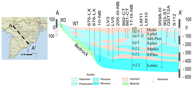
Figure 3 The setting and hydrogeological features, including aquifer names, of the Mekong Delta, Vietnam, with the locations of the cross sections A–A^′ (from Doan et al., 2016). Map copyright: © National Geographic, Esri, Garmin, HERE, UNEP-WCMC, USGS, NASA, ESA, METI, NCRAN, GEBCO, NOAA, increment P Corp.

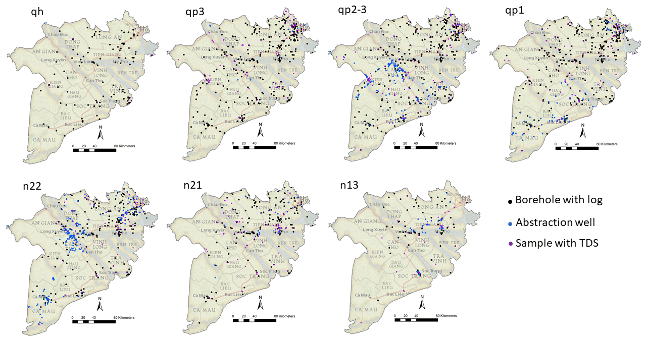
Figure 4 Spatial distribution of the used data that are applied for each aquifer. The data density for the deepest aquifer – n13 – is not sufficient to produce adequate estimates of groundwater salinity concentrations and is therefore discarded from further analysis. Map copyright: © National Geographic, Esri, Garmin, HERE, UNEP-WCMC, USGS, NASA, ESA, METI, NCRAN, GEBCO, NOAA, increment P Corp.

2.4 Data processing

In this section, the available data and the data transformation techniques that are used are described to arrive at a dataset that is input for spatial interpolation and simulation. The main data sources are the boreholes with the description of lithology and resistivity, supplemented by both industrial and domestic abstraction wells.

2.4.1 Data collection

The database of the Division of Water Resources Planning and Investigation for the South of Vietnam (DWRPIS) was queried to obtain relevant data for the modelling of each hydrogeological unit and groundwater salinity distribution (TDS): 378 borehole descriptions with geophysical loggings and lithological description of the sediments, 732 industrial abstraction wells, and 407 groundwater samples that contained TDS concentrations. The data were collected during the 1980s until 2015 and were interpreted into hydrogeological units by hydrogeologists of DWRPIS. The borehole interpretation was aided by natural gamma measurements that were collected in the borehole; temperature and bulk electrical resistivity were also recorded. In Fig. 4 the spatial distribution of the data is shown for each aquifer. Due to limited data for aquifer n13, this aquifer was excluded from further analysis. The borehole data were aggregated into 1 m intervals, for reasons of efficiency and to obtain a more uniform dataset. This aggregation was done with respect to the borders of the hydrogeological units so that no aggregation occurs over the borders of different units. The variables that were used for further analysis include lithological description, long normal (LN64) resistivity (also called bulk resistivity, representing the resistivity of the sediments and the groundwater), the temperature of the groundwater and classification into hydrogeological units; see Fig. 5 for an examples of a typical geophysical log.

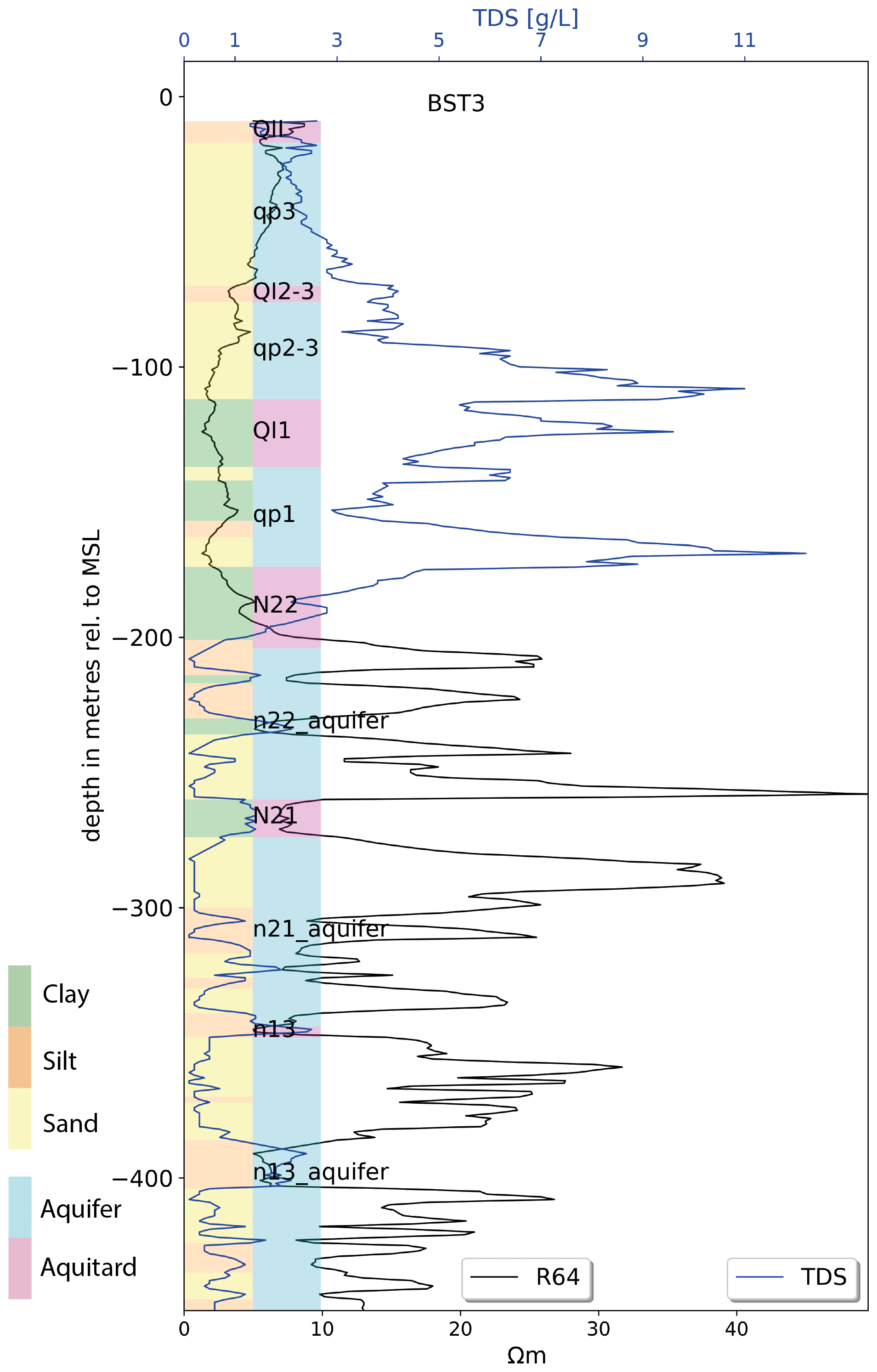
Figure 5 Typical geophysical logs (black line) and borehole description, resulting in TDS concentrations (blue line).

2.4.2 From borehole logging to TDS

The intrinsic formation factor (F_i) relates the bulk resistivity of a fully saturated granular medium to the fluid resistivity. Archie (1942) defined F_i as the ratio of bulk resistivity over fluid (water) resistivity (${\mathit{\rho }}_{\text{bulk}}/{\mathit{\rho }}_{\text{w}}$), which is valid for clay-free, consolidated sediments. However, the sediments in the Mekong Delta are not clay-free and are unconsolidated, rendering the use of Archie's formula invalid, as discussed by for example Huntley (1986) and Worthington (1993). For clayey, unconsolidated sediments, the ratio of bulk resistivity over fluid resistivity is called the apparent formation factor, F_a. A modification of the Archie equation is proposed by Huntley (1986) and Worthington (1993) and applied by for example Soupios et al. (2007), to obtain F_a. The procedure that was used includes the determination of a lithology-specific relation between ρ_w and $\mathrm{1}/F_{\text{a}}$. Groundwater resistivity was determined from an independent dataset relating measured TDS to electrical conductivity of the groundwater. In Appendix B the procedure to obtain F_a is described in detail, as well as the validation of the resulting F_i using an independent dataset. The resulting F_i for each lithology is used to convert LN64 to ρ_w.

Table 1 Formation factor and drainable porosity for lithology classes. The intrinsic formation factor (F_i) from literature (De Louw et al., 2011; Faneca Sànchez et al., 2012) and in brackets F_i as checked by comparison with TDS–Ec(groundwater) data from Buschman et al. (2008) and An et al. (2014). Drainable porosity based on Johnson (1967).

To obtain TDS from ρ_w, a regression between the electrical conductivity (Ec, reciprocal of ρ_w) and TDS was established, based on the 55 samples with TDS and ρ_w (Fig. 6). This regression was applied to all 1 m intervals in the boreholes with LN64 measurements – in total 81 250 m – resulting in 36 % of the in intervals in the boreholes having TDS < 1 g L⁻¹ and 68 % < 3 g L⁻¹ (cumulative).

2.4.3 Additional (soft) data sources of TDS estimates

Industrial extraction wells

The DWRPIS database contains data from industrial extraction wells that extract groundwater in excess of 200 m³ d⁻¹. These wells often produce large volumes of drinking water for villages and towns and for industrial and agricultural purposes. The depth and the aquifer from which the groundwater is extracted are stored in the database. Only a small part of these wells was tested by the local authorities or by the well owners for compliance with the national standards. After consultation with the local experts, it was decided to set TDS of these extraction wells in the database to 0.3 g L⁻¹.

Figure 6 Linear regression between electrical conductivity of groundwater and TDS.

Domestic extraction wells

There are a large number of households in the MKD that have their own groundwater well for domestic use. Most of these wells are drilled by local companies and are unregulated. The location, depth and volume of groundwater extracted are not known. DWRPIS has carried out an investigation to obtain basic data – location of wells and the aquifer from which the groundwater is extracted – for part of these wells in 2010; see Fig. 7 (Bui et al., 2013). No data on the quality of the water or the depth of extraction are available. To obtain the depth interval from which the water is extracted, the average depth interval – relative to the top of the aquifer – from the boreholes that contain TDS < 1 g L⁻¹ in the corresponding aquifer for that area was calculated. This average depth interval was subsequently used as a proxy for the depth interval for the domestic wells. The extracted groundwater is used for domestic purposes and was therefore assumed to have a TDS < 1 g L⁻¹. The locations of domestic extraction wells are extremely dense and clustered. The domestic extraction data were aggregated into averages of 5000 × 5000 m to prevent the abundant domestic well data from overwhelming the other TDS data. The presence of the domestic extraction wells is of great importance for increasing the spatial coverage of the data to estimate the TDS distribution in the MKD. Although the TDS of the domestic extraction wells is only approximately known, the high density of the wells and its spatial extent renders these data extremely valuable.

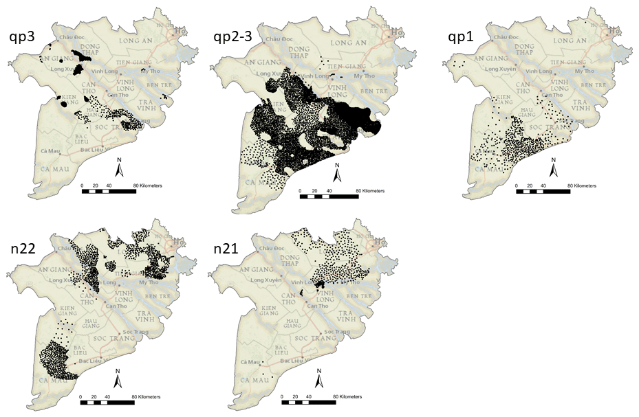
Figure 7 Spatial distribution of domestic extraction wells in the MKD, with known location and aquifer from which the groundwater is extracted. No data for the Holocene aquifer, qh, are available because of its predominant brackish/saline nature. Map copyright: © National Geographic, Esri, Garmin, HERE, UNEP-WCMC, USGS, NASA, ESA, METI, NCRAN, GEBCO, NOAA, increment P Corp.

2.4.4 Drainable porosity

To determine the amount of potential extractable groundwater from each aquifer, the spatially distributed drainable porosity is needed. Drainable porosity indicates the part of the total volume of an aquifer that drains under gravity (Fitts, 2002) and is also called effective porosity. It is presented as a volume ratio and is thus dimensionless. Data for drainable porosity of aquifers in the MKD are limited. To derive at a spatial differentiated model (2D map) of drainable porosity for each aquifer, each lithological interval in the boreholes was assigned a drainable porosity depending on the characteristics of the sediments, as described in the DWRPIS database. By aggregating over the lithological intervals, an average drainable porosity was calculated at each borehole location within the aquifer and subsequently interpolated to derive a map of drainable porosity for the entire extent of each aquifer. The procedure is described in detail in Appendix C. The drainable porosity per lithological class is taken from Johnson (1967); see Table 1. The resulting drainable porosity maps are unique, in the sense that previous models of the geohydrology in the MKD either do not model drainable porosity (Minderhoud et al., 2017) or average drainable porosity per province (Bui et al., 2013).

2.5 Three-dimensional modelling of aquifers and aquitards

To estimate the spatially distributed fresh groundwater volume – including uncertainty – in each aquifer of the MKD, a model of the top and bottom of each hydrogeological unit in the subsurface is required. Minderhoud et al. (2017) constructed - based on 95 boreholes – a hydrogeological model (cell size 1000 × 1000 m²) of the MKD. The larger dataset used in this study consists of the interpreted base of the hydrogeological units from boreholes and extraction wells (Fig. 4). These were used to update the basic model to a new, more detailed model by kriging the base of each unit and consequently stacking the units in the right stratigraphical order to obtain a consistent model. The procedure is described in detail in Appendix D. The resulting layer model was converted into a voxel model (dimensions of the voxel: 1000 m × 1000 m × 5 m³) by assigning the appropriate hydrogeological unit to each voxel. The top of the voxel model was formed by the digital elevation model (DEM), derived from Minderhoud et al. (2017).

3 Results

3.1 Three-dimensional model of aquifers and aquitards

Figure 8 presents the updated hydrogeological model of the aquifers (lower-case names) and aquitards (upper-case names) in the study area up to a maximum depth of 600 m. The model depicts considerable detail, showing aquifers that can have thicknesses up to tens of metres. The main difference with the previous hydrogeological model (Minderhoud et al., 2017) is that due to a substantial larger amount of data more detail is present.

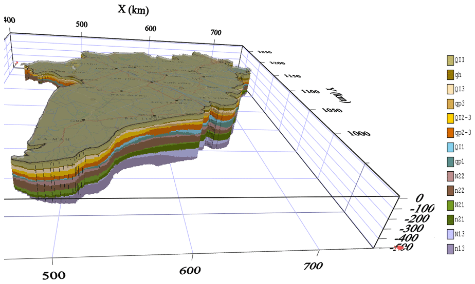
Figure 8 Updated hydrogeological block model. Scale according to kilometre reading along the axis (km) and depth in metres. Vertical exaggeration: 100×.

Figure 9 Statistical distributions of TDS for each aquifer.

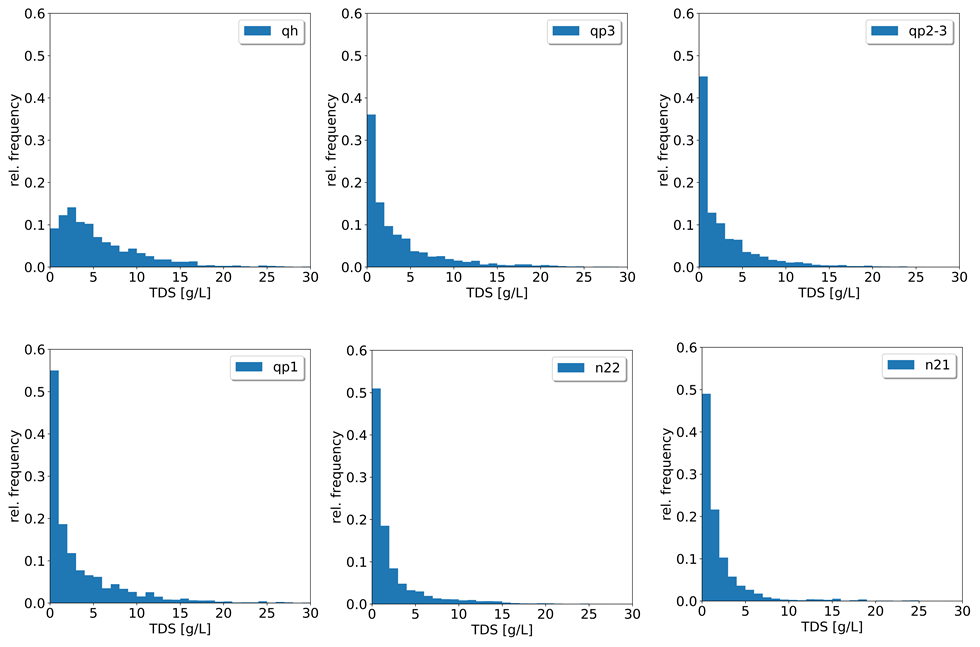
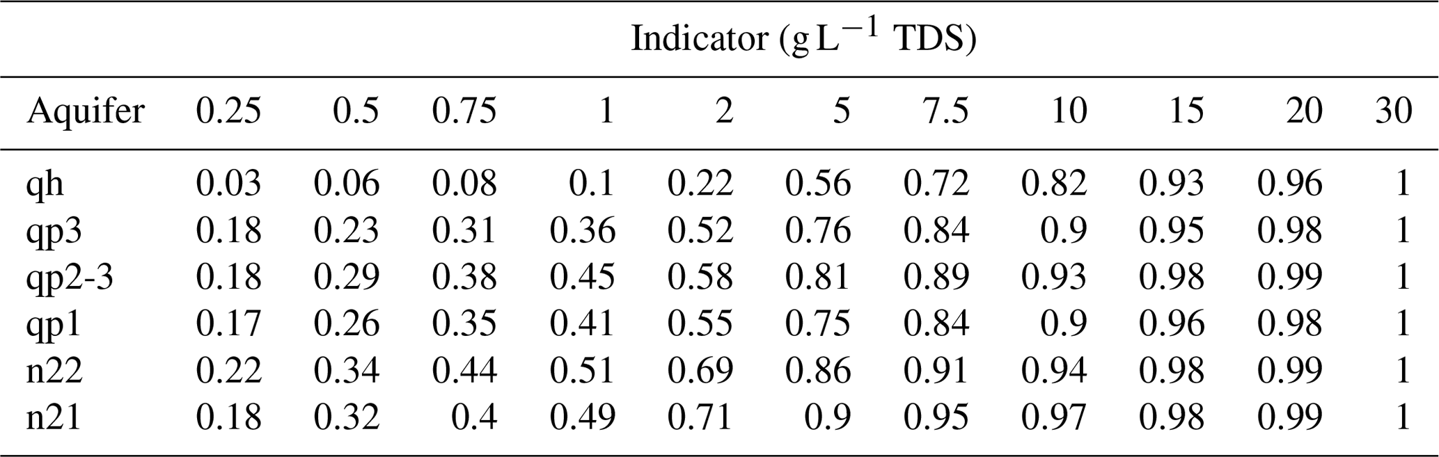
Table 2 Cumulative probabilities at indicator thresholds for each aquifer.

3.2 Geostatistical analysis of TDS

3.2.1 Statistical distribution of TDS data and indicator coding

Figure 9 shows the frequency distribution of TDS for each aquifer based on the TDS derived from the boreholes with geophysical logging, groundwater samples and data from industrial extraction wells. TDS vary between the different aquifers and also between the aquifers and aquitards of the same hydrogeological unit (data of the aquitards not shown here). Formal statistical testing using the Mann–Whitney U test, a nonparametric equivalent of the t test of the equality of the mean of two samples (Davis, 2002), shows that almost all TDS across the six aquifers differ at the p=0.05 level, except between the Middle Pliocene (n22) and Early Pliocene (n21) aquifers. Also, TDS in the aquifer and aquitard from the same hydrogeological unit are statistically different at the p=0.05 level (data not shown). Based on this, it was decided to apply the geostatistical modelling and interpolation of TDS separately for each individual aquifer and aquitard. The reason why the hydrogeological units have different statistical distributions of TDS is not clear yet. It could be due to different cycles of freshening of the erstwhile saline groundwater (Pham et al., 2019) or due to the fact that mixing of saline and fresh groundwater is not uniform over the MKD. The focus of the remainder of the analysis is on the aquifers, since the main objective of the study is to assess fresh groundwater volumes. The analysis and interpolation that is reported for the aquifers is also carried out for the aquitards to obtain a 3D groundwater salinity distribution of the groundwater in the subsurface of the entire MKD, but details are not reported here. The results are shown in Fig. 11.

The data from the industrial extraction wells, which were uniformly set at TDS of 0.3 g L⁻¹, will cause complications due to the spike in the histogram at 0.3 g L⁻¹. Furthermore, the incorporation of “soft”, incomplete data from the domestic extraction wells needs to be considered, which is difficult to achieve in a parametric setting. Indicator geostatistics allows for the incorporation of incomplete, soft data by coding these into indicator values. Therefore, the indicator approach is used, in which each observation is transformed into a set of K indicator values, corresponding to K threshold values. The threshold values are chosen to coincide with important TDS intervals and with more emphasis on the low TDS since that determines the quality of drinking water and usability for irrigation purposes and aquaculture. The first two threshold (0.25 and 0.50 g L⁻¹) are half the recommended limit and the recommended limit for drinking water by the EPA (https://www.epa.gov/); 1.0 g L⁻¹ is the freshwater threshold in Vietnam and 3.0 g L⁻¹ represents the brackish water threshold. The full list of TDS indicators and their corresponding fraction at each indicator thresholds and for each hydrogeological unit is given in Table 2. The domestic well dataset was treated as soft data in the data analysis, interpolation and simulation procedure. Because the domestic wells represent incomplete data – TDS concentrations are only known to be lower than 1.0 g L⁻¹ – the indicator coding was performed to take this into account. So, only the indicator that represents the threshold of 1.0 g L⁻¹ was coded, while the rest of the indicator thresholds were assigned as missing data. This will prevent bias that might arise from using the incomplete domestic well data, since the indicator kriging procedure is informed that only the information about the fact that TDS is < 1 g L⁻¹ is to be used. This also applies for the industrial extraction wells, in which case the threshold of 0.3 g L⁻¹ was used.

In certain areas, clusters of TDS data occur; see Fig. 4. Preferential clustering of data is detrimental to unbiased estimation, and declustering is advised (Deutsch, 2002). Declustering was performed by averaging all TDS values that occur in a voxel of 1000 × 1000 × 5 m³. This also serves to eliminate short-distance variation obscuring the regional variation. The remainder of the research described here proceeds with the declustered TDS dataset. Declustering of the data for the domestic wells was performed on a 5000 × 5000 m² grid spacing.

3.2.2 Estimation of indicator semivariograms

The geostatistical interpolation technique (indicator kriging) calls for semivariogram models for each indicator threshold to estimate the complementary cumulative distribution function of TDS at each location (voxel). The semivariograms were estimated for the median indicator of the TDS distribution (1 g L⁻¹) using the declustered data, in which the smallest horizontal distance between data points is 1000 m (horizontal dimension of the voxel). Appendix E describes the procedure for calculating the semivariograms and the interpretation of the results.

3.2.3 Cross-validation

As described in Sect. 3.2.1, TDS data were averaged over each voxel, resulting in vertical columns of voxels (voxel stacks) that contain TDS data that were used as input for the interpolation. To evaluate the accuracy of the interpolation, a cross-validation is carried out by discarding (for each individual aquifer) an entire stack of voxels with known TDS. Next, the CCDF of TDS for each voxel in the discarded stack is estimated. The final result of the indicator kriging cross-validation is an estimated CCDF for each 5 m interval in the cross-validated voxel stack. Since the actual TDS value is known, the performance of the interpolation can be evaluated. In this section, the results of the cross-validation for aquifer qp2-3 is given; Appendix F describes the results of the cross-validation for each aquifer. In Fig. 10 results are summarized in scatterplots and graphs.

The scatterplot (upper left panel) present the true vs. the estimated TDS (according to the E-type estimate), the correlation coefficient (r) and the mean absolute error (MAE). The data contain large values of TDS that can have a great impact on the magnitude of MAE. To further evaluate the results of the cross-validation, plots and bar charts are presented.

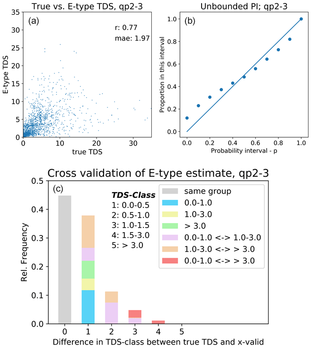
Figure 10 Results of the cross-validation for aquifer qp2-3. Panel (a) shows scatterplot of true versus E-type TDS estimates; panel (b) indicates the accuracy of the interpolation by proportion of data that fall in a certain probability interval (PI); panel (c) shows the summary of the cross-validation results concerning grouping of TDS values. For further explanation refer to the main text.

The accuracy plot (top right, Fig. 10) shows the expected proportions versus the estimated proportions in 10 probability exceedance intervals (Goovaerts, 2001). In the lower probability intervals (up to probability interval 0.5) the estimated proportions deviate from the theoretical proportions, indicating that the probabilistic model for the lower probabilities is less accurate. Since the main interest is in the higher probabilities (e.g. probability that TDS exceeds 1 g L⁻¹ > 0.5), this is not regarded as problematic.

The last check concerning the performance of the interpolation was done by classifying TDS into five classes: 0–0.5, 0.5–1, 1–1.5, 1.5–3 and > 3 g L⁻¹. Next, it was calculated to what extent the actual and the estimated (E-type) differ (difference in TDS class between data and cross-validation) and, if so, whether the difference is causing the sample to fall in another group. The grouping was done following important TDS values for water use: 0–1 g L⁻¹ (fresh), 1–3 g L⁻¹ (brackish) and > 3 g L⁻¹ (saline). This analysis shows that around 70 % of the estimated TDS falls in the same group, although there are some differences in classes. The number of estimated TDS that cross from fresh to saline (and vice versa) is limited, and this is also the case from fresh to brackish.

Note that by allowing instrumental parameters in the interpolation to vary (e.g. neighbourhood for interpolation, minimum and maximum number of samples in the interpolation), an optimal set of these parameters was determined such that the cross-validated results were “best” (these are the results depicted in the graphs). No rigorous evaluation of all possible combinations of parameters was performed, but the parameters were varied within reasonable limits, and the results were checked using graphs and correlation coefficients.

3.2.4 Three-dimensional modelling of TDS

Three-dimensional indicator kriging is used with TDS indicator data derived from the boreholes, groundwater samples, and industrial and domestic extraction wells as input, resulting in a 3D model of the CCDF of TDS for each voxel, from which the expected value of TDS (E-type estimate) was calculated. The probability that TDS is less than a certain threshold (e.g. 1 g L⁻¹ TDS) is easily computed and is also shown.

The 3D distribution of fresh–brackish–saline groundwater (classified from the E-type estimate of TDS) for the aquifers and aquitards in the MKD is depicted in Fig. 11 (left panel). The TDS were classified in three classes: 0–1 g L⁻¹ (fresh), 1–3 g L⁻¹ (brackish) and > 3 g L⁻¹ (saline). Together with the probability of TDS < 1 g L⁻¹ (right panel), this gives detailed information about the occurrence of fresh groundwater and its uncertainty.

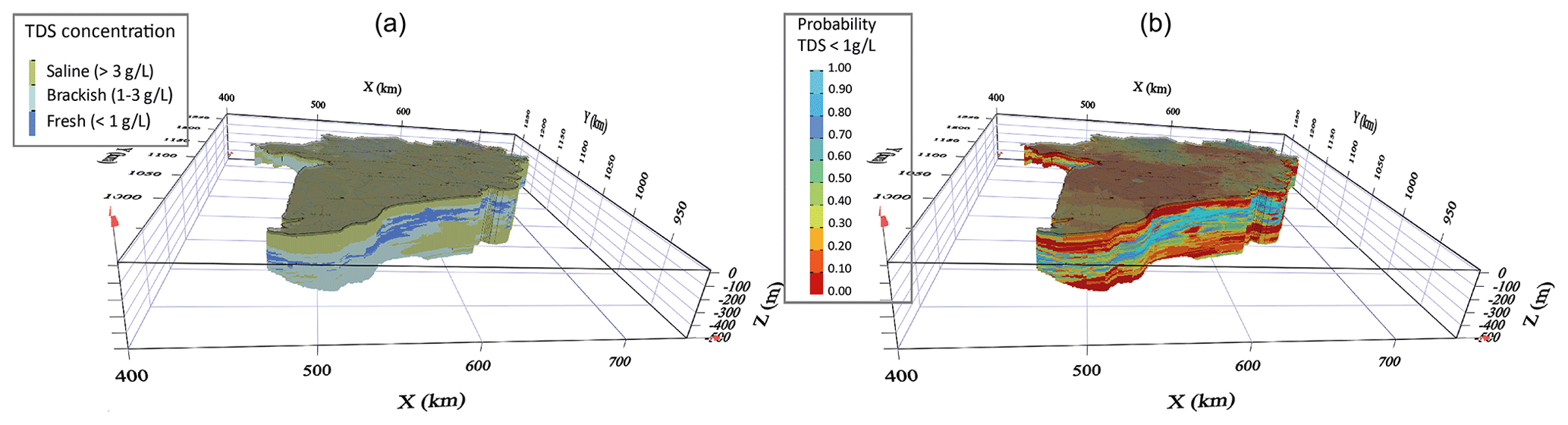
Figure 11 The 3D perspective view of the spatial distribution of fresh–brackish–saline groundwater (a) and the probability that TDS < 1 g L⁻¹ (b).

The 3D model of the CCDF of TDS allows for the inspection of the fresh groundwater distribution for each individual aquifer. In Fig. 12 the models of the spatial distribution of TDS are given, again together with the probability of TDS < 1 g L⁻¹. In some areas, large variations in TDS are modelled over relatively short distances. One reason might be the occurrence of the so-called salt water “fingering” occurring in a heterogeneous (3D) distribution of lithology that is caused by variable-density groundwater flow during erosion and sedimentation cycles in paleo-times (e.g. Delsman et al., 2014; Larsen et al., 2017; Pham et al., 2019; Zamrsky et al., 2020). Another reason is that aquifers are incised into sediments that formed aquitards. The modelling of TDS occurred separately in aquifers and aquitards, thereby creating sometimes sharp boundaries in TDS concentration. And in certain areas data sparsity might cause artefacts in the model. The user of the model is reminded that the main aim of this study is to estimate freshwater occurrence and volumes. Therefore, the use of the three classes of salinity (fresh, brackish, saline), together with the probability of TDS < 1 g L⁻¹ (Fig. 11), is valuable for this purpose, while the E-type estimate can be used for further analysis and modelling that requires TDS.

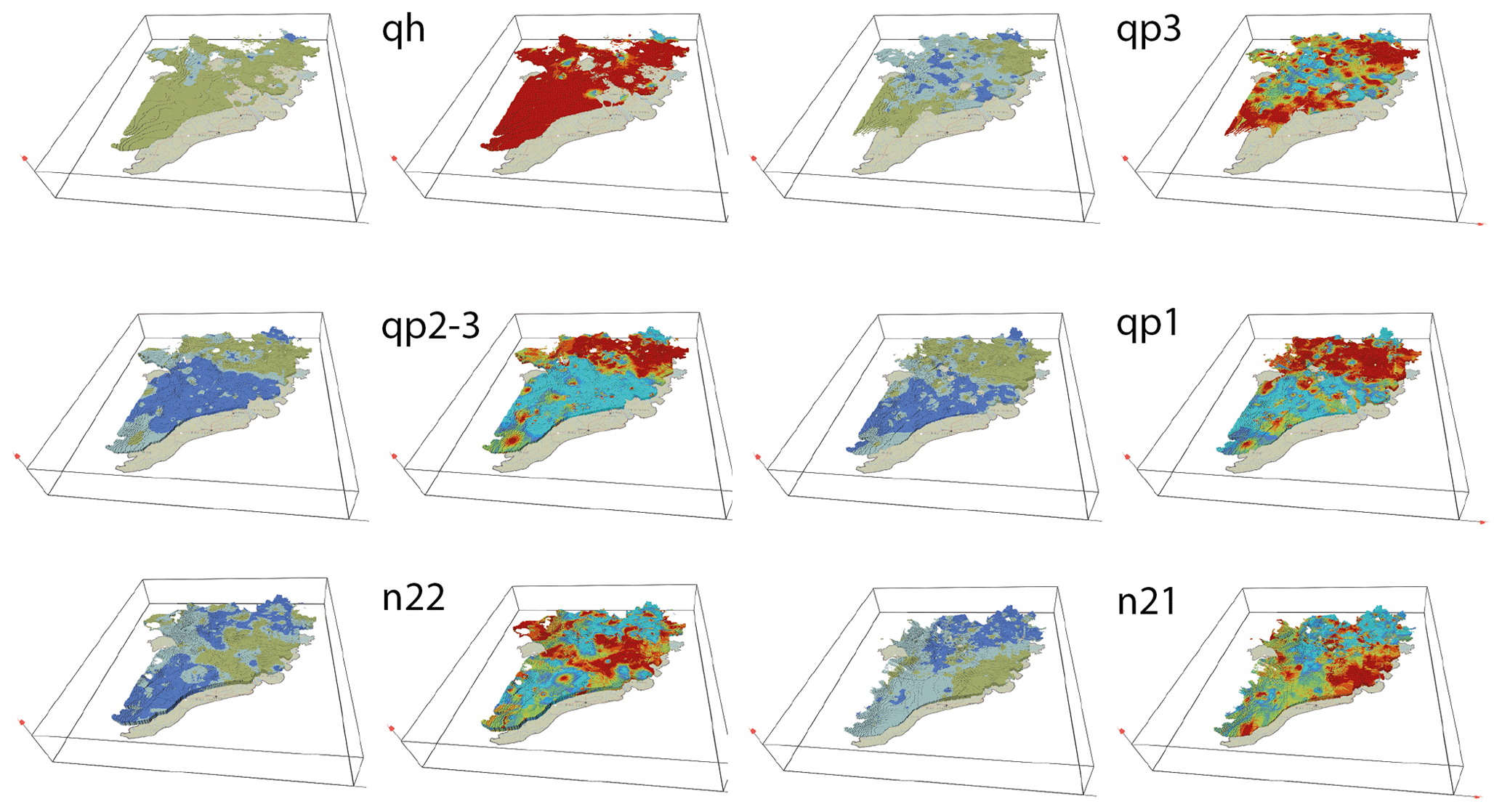
Figure 12 Three-dimensional perspective view of the spatial distribution of fresh, brackish and saline (left panels) and the probability that TDS < 1 g L⁻¹ (right panels) for the aquifers in the area. For legend see Fig. 11.

3.2.5 Estimating the fresh groundwater volume from indicator kriging

For each location (x,y) in each aquifer the expected volume of fresh groundwater was estimated from the CCDF of TDS for each voxel in the stack and the layer-averaged drainable porosity. Assuming an upper limit for TDS of 1 g L⁻¹,

$$\begin{array}{}\text{(1)}& \begin{array}{rl}& E\left[{\mathrm{Volume}}_{\text{aquifer}}(x,y)\right]=\\ & \left\{\sum _{z_{\text{bottom}}}^{z_{\text{top}}}\text{Prob}\mathit{\{}\left(\text{TDS}(x,y,z)\right)<\mathrm{1}\mathrm{g}{\mathrm{L}}^{-\mathrm{1}}\mathit{\}}\times {\text{Volume}}_{\text{voxel}}\right\}\\ & \times \text{Drainable Porosity}(x,y).\end{array}\end{array}$$

This results in the expected fresh groundwater volume at every location (Fig. 13). Adding expected volumes for each location results in the expected volume for the entire aquifer (Table 3). The total expected volume for all the aquifers considered is 867 billion cubic metres, which is considerably larger than a previous (most recent) estimate of 600 billion cubic metres (Bui et al., 2013). The difference between the estimates can be attributed to the fact that the previous method used an estimate of the total area of fresh water for each aquifer and a significant smaller value for drainable porosity. Also, in the previous method, averages of thickness for each aquifer per province were used, thereby ignoring the intra-regional spatial variation that is obviously present.

Table 3 Volume of fresh groundwater for each aquifer (TDS < 1 g L⁻¹) in billion cubic metres.

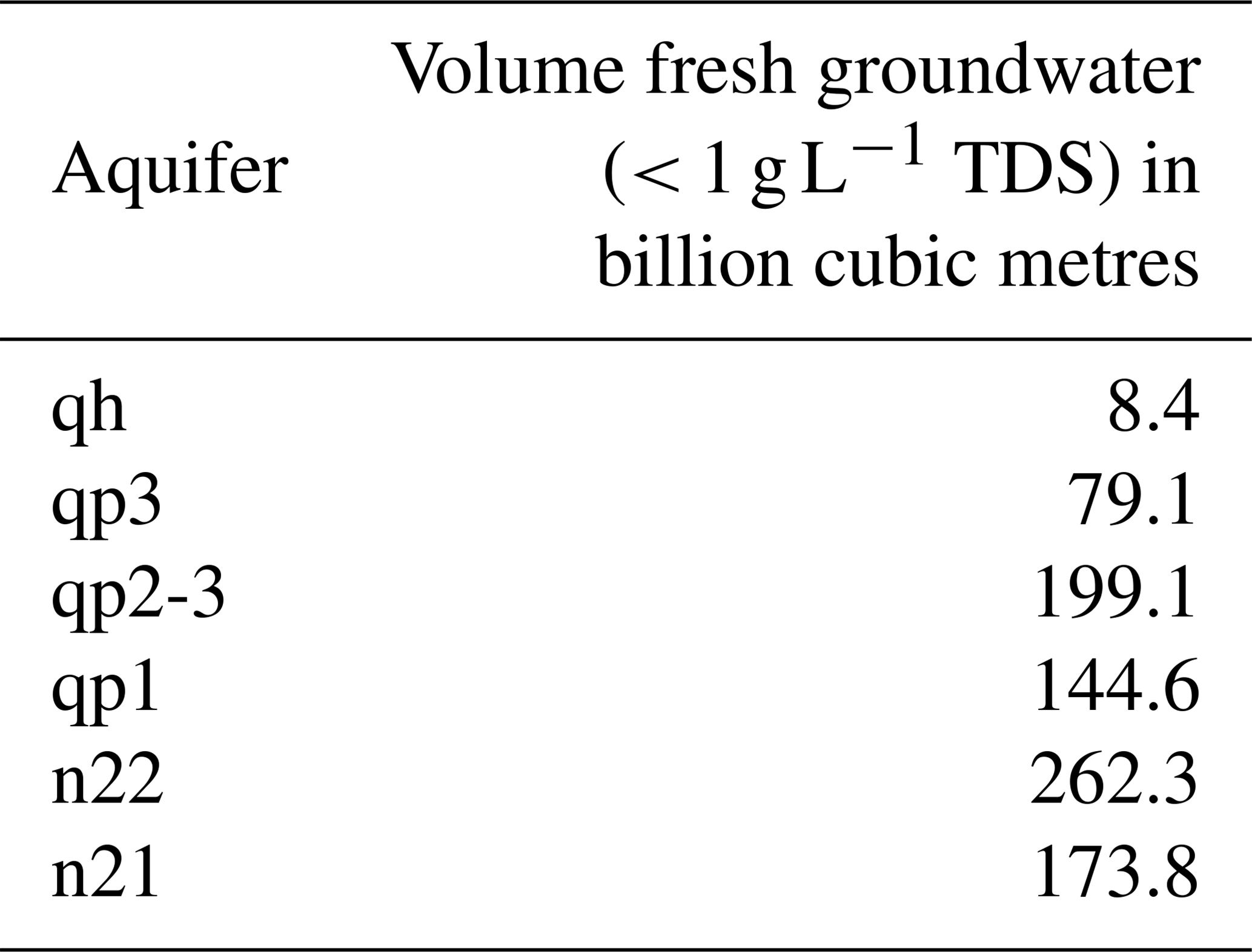
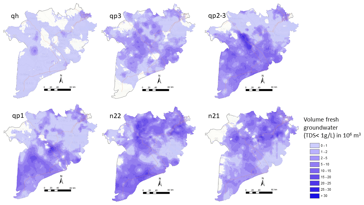
Figure 13 Maps showing the expected depth-averaged volume of fresh groundwater in the aquifers, per 1 × 1 km² model cell. In blank areas the aquifer is not present.

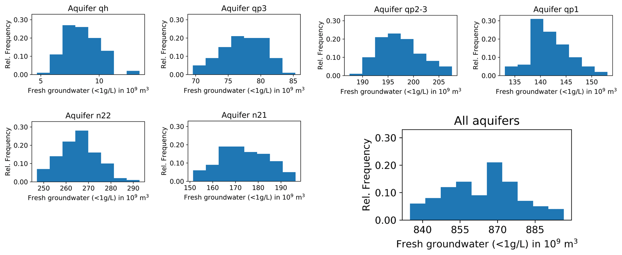
Figure 14 Estimated volumes of fresh groundwater (TDS < 1 g L⁻¹) for each aquifer and for all aquifers combined, based on 100 Monte Carlo realizations obtained by indicator simulations. Note that the units on the horizontal axes vary.

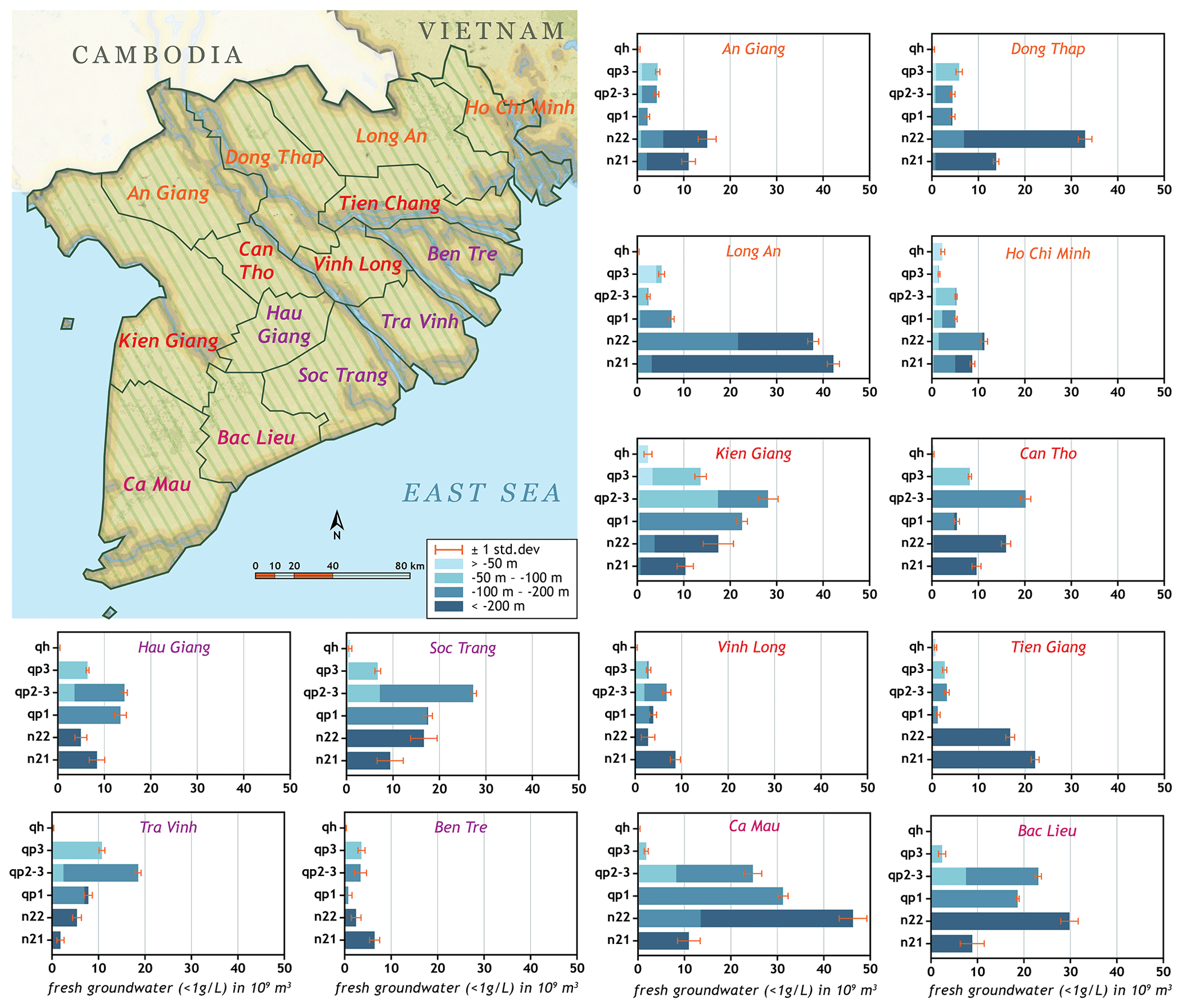
Figure 15 Volume of fresh groundwater in the aquifers for each province and depth interval (relative to m.s.l.), including uncertainty. Map copyright: © National Geographic, Esri, Garmin, HERE, UNEP-WCMC, USGS, NASA, ESA, METI, NCRAN, GEBCO, NOAA, increment P Corp.

3.2.6 Uncertainty estimates of fresh groundwater volumes with indicator simulation

The fresh groundwater volume for each aquifer, as estimated with indicator kriging of TDS and drainable porosity, results in an expected value at each location, but without an indication of the uncertainty for the entire volume of the aquifer. To obtain an estimate of the uncertainty of the volumes of fresh groundwater for each aquifer, sequential indicator simulation was used to produce 100 realizations of the conditional random function of TDS for each aquifer. Again, next to the “hard” borehole and industrial extraction well data, soft data from the domestic extraction well dataset were used. The parameters that were used for indicator kriging (semivariogram model, neighbourhood, etc.) were also used in simulation. For each of the 100 realizations, the volume of fresh groundwater (groundwater volume of cells with simulated TDS < 1 g L⁻¹) was determined, resulting in 100 samples of fresh groundwater volumes for each aquifer. The resulting histograms for each aquifer are depicted in Fig. 14. As expected, the average fresh groundwater volume for each aquifer, as calculated from indicator simulation, is approximately the same as resulting from indicator kriging results. The range of uncertainty is largest for the deeper aquifers, having the lowest data density.

The uncertainty estimates of the fresh groundwater volumes calculated in this way only account for the spatial uncertainty of the TDS. Other sources of uncertainty, such as the uncertainty in the formation factor, drainable porosity and interpretation of the boreholes in hydrogeological units, are not considered.

3.2.7 Assessing regional groundwater volumes

The estimated volume of fresh groundwater for each province was determined for each aquifer and for a range of depth intervals (relative to m.s.l.): < −50, −50 m to −100 m, −100 m to −200 m and < −200 m. In Fig. 15 the results are presented, together with the uncertainty, based on indicator simulation. There is considerable variation in the availability of fresh groundwater over the provinces and depth ranges.

4 Data availability

The downloadable hydrogeological and TDS model, available at https://doi.org/10.5281/zenodo.4441776 (Gunnink et al., 2021), contains the following files:

• “hydrogeology_Mekong_Vietnam.nc” with the variable “hydrogeological_unit”, representing aquifers (lower case) and aquitards (upper case), with the naming convention according to Fig. 8 and the description in Appendix D;

• “TDS_Mekong_Vietnam.nc”, which contains the variables

  • “Etype_estimate_TDS”, representing TDS concentration (in g L⁻¹);

  • “Fresh_brackish_saline”, in which each voxel is classified as containing fresh (TDS < 1 g L⁻¹), brackish (TDS 1–3 g L⁻¹) or saline groundwater (> 3 g L⁻¹);

  • “Probability_TDS_smaller_1g_L”, representing the probability that TDS < 1 g L⁻¹.

5 Conclusions

For the Mekong Delta, Vietnam, data from various sources (boreholes with geophysical loggings, groundwater samples, industrial extraction wells and data from domestic wells) were combined to produce a 3D model of the CCDF of TDS, representing the groundwater salinity distribution. The first step was to construct a 3D hydrogeological model so that the groundwater salinity modelling could proceed within the constraints of the fresh groundwater volume of each aquifer and aquitard. By using the geostatistical interpolation technique indicator kriging, it was possible to combine TDS data from different sources and quality to produce a CCDF of TDS at each ($x,y,z$) location. The results of the interpolation and simulation indicate that there is a sizable fresh groundwater volume in the MKD area (an expected value of 867 billion cubic metres, with an uncertainty range of 830–900 billion cubic metres). There is considerable spatial variability in TDS, and the uncertainty in volumes is the largest for the deeper aquifers. A groundwater salinity model containing both TDS concentrations and uncertainties can be used as a tool for the management of fresh groundwater reserves and can help to promote and manage sustainable use of this precious freshwater source.

The fresh groundwater volume seems to be huge, in comparison with the present yearly groundwater extraction rates for industrial, domestic and agricultural water use. However, it is important to recognize that in areas where replenishment is very limited, these extraction rates can cause rapid upconing of brackish to saline groundwater. Mixing of fresh groundwater with brackish and/or saline groundwater is a serious threat to the fresh groundwater volume, resulting in an apparently modest groundwater extraction regime easily becoming non-sustainable. The current model can be updated when new data become available, because the calculation workflow is flexible in a sense that data from a range of sources can be incorporated, as long as the data can be reasonably linked to groundwater quality (or drainable porosity).

Appendix A: Hydrogeological schematization in the MKD

A highly heterogeneous stratigraphy was formed in the MKD as a result of repeated transgression and regression events from the late Neogene to the present. The Pleistocene and Holocene sediments are of fluvial and deltaic origin, while Miocene and Pliocene sediments are of marine origin (Bui et al., 2013). The sediments in the MKD can be divided into seven geological units (Minderhoud et al., 2017; Pham et al., 2019). Each geological unit consists (in general) of a lower part of fine to coarse sand (aquifer) and an upper part of silt, sandy clay and clay (aquitard). The hydrogeological schematization of aquifers and aquitards in the MKD is depicted in Fig. 3. According to the Vietnamese nomenclature (Bui et al., 2013; Nguyen et al., 2004), the seven aquifers (lower case)/aquitards (upper case) in the study area are the Holocene (qh/QII), Late Pleistocene (qp3/QI3) , Late–Middle Pleistocene (qp2-3/QI2-3), Early Pleistocene (qp1/QI1), Middle Pliocene (n22/N22), Early Pliocene (n21/N21) and Late Miocene (n131/N13). The MKD unconsolidated sediments are very thick, especially near the coast where between the two main rivers thicknesses of up to nearly 600 m are observed (Nguyen et al., 2004). For reference, only 0.3 % of the coastal aquifers in the world are estimated to exceed this thickness (Zamrsky et al., 2018).

Appendix B: Formation factor

The intrinsic formation factor (Archie, 1942) – F_i – is only valid for clay-free, clean, consolidated sediments. For unconsolidated, clayey sediments, the apparent formation factor – F_a – is defined as the ratio of bulk resistivity over fluid resistivity. A modification of the Archie equation is proposed by Huntley (1986) and Worthington (1993) and applied by for example Soupios et al. (2007) and Faneca Sànchez et al. (2012), to obtain F_a.

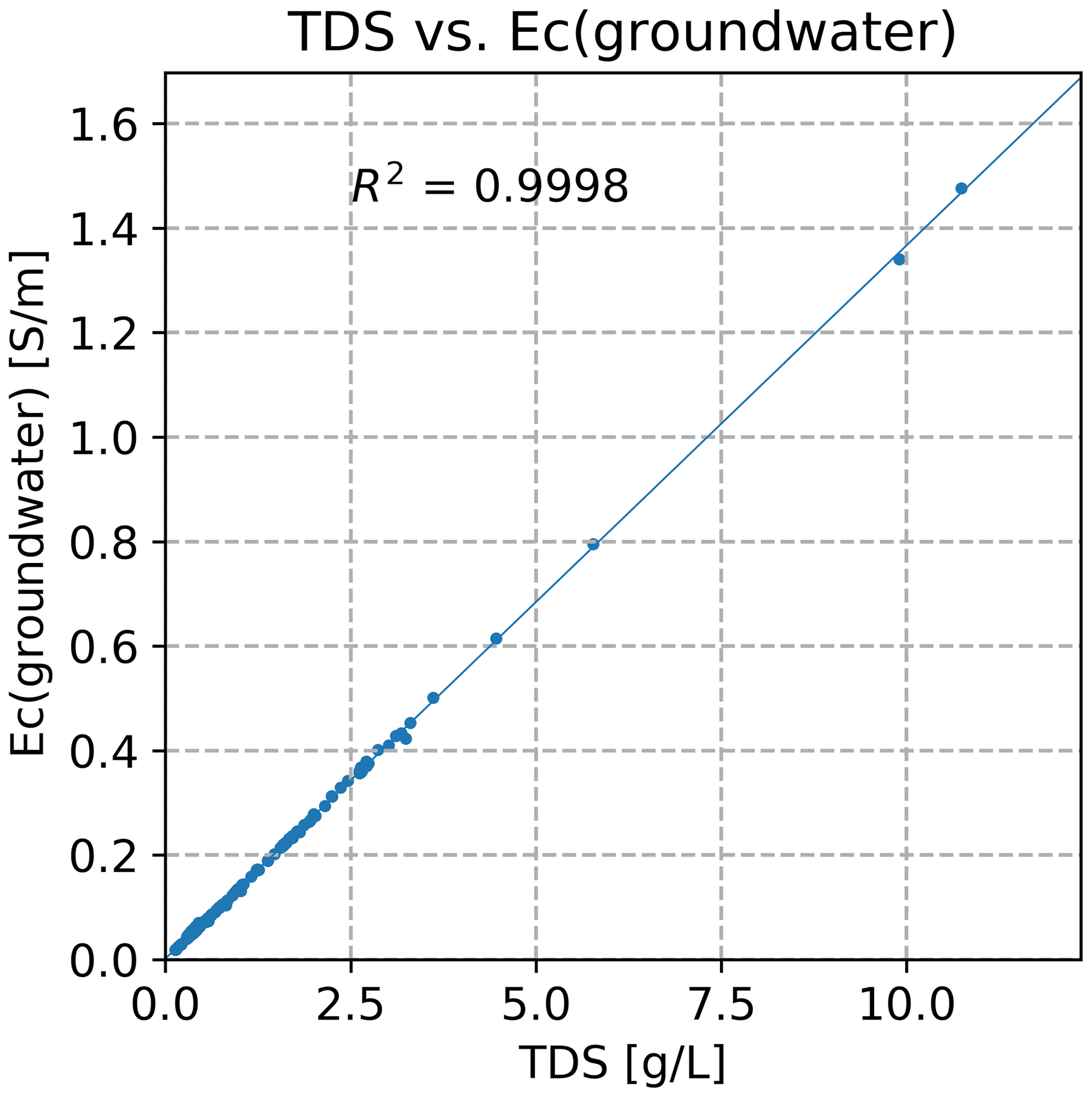
Figure B1 Linear relation between TDS and Ec(groundwater), based on data from Buschmann et al. (2008) and An et al. (2014).

The relation between F_i and F_a is given by

$$\begin{array}{}\text{(B1)}& \mathrm{1}/F_{\text{a}}=\mathrm{1}/F_{\text{i}}+(B{Q}_v/F_{\text{i}})\times {\mathit{\rho }}_{\text{w}},\end{array}$$

where BQ_v [Ω m] is related to the effects of surface conduction, mainly due to clay particles, and ρ_w is the resistivity of the groundwater [Ω m]. When plotting $\mathrm{1}/F_{\text{a}}$ vs. ρ_w, the intercept of the straight line with the y axis will result in $\mathrm{1}/F_{\text{i}}$, and BQ${}_v/F_{\text{i}}$ represents the gradient. Since there are no data of F_i available for the sediments in the Mekong Delta, published data from De Louw et al. (2011) and Faneca Sànchez et al. (2012) were used. These F_i values were determined in unconsolidated Holocene and Pleistocene sediments in the Rhine–Meuse delta Netherlands, which is thought to be applicable to the Mekong Delta sediments, due to the similarity in depositional environments and lithology in both deltas.

The F_i values were checked for validity in the following way. The dataset from DWRPIS contains lithology, TDS and LN64 (bulk resistivity) for 55 depth intervals, covering the main hydrogeological units and lithologies therein in the MKD, but the dataset contains no data on groundwater resistivity, ρ_w.

Buschmann et al. (2008) reported data on TDS and ρ_w in the Mekong Delta of Vietnam, for 112 samples with an average sampling depth of 70 m (range 10–420 m). An et al. (2014) collected 22 samples of TDS and ρ_w in a coastal area in the eastern part of the Mekong Delta from depths 80–130 m. These two datasets were merged, and a linear regression between TDS and electrical conductivity (Ec) of the groundwater (the reciprocal of ρ_w and corrected for temperature, according to TNO-IGG, 1992) is established (Fig. B1). This regression is applied to the measured TDS in the DWRPIS database to derive (again, after correction for temperature) ρ_w. This allows for the calculation of the apparent formation factor, F_a.

The formation factor depends on the lithology of the sediments, especially the clay content. The applicability of the published F_i in this study was checked for each lithology class by applying the relation of Fig. B1 to the measured TDS to obtain ρ_w and subsequently obtaining $\mathrm{1}/F_{\text{a}}$ for the lithological units of Table 1; see Fig. B2.

There is scatter in most of the graphs, caused by variability in grain size of the sand fraction, clay content and facies change. In general, F_i derived from the analysis depicted in Fig. B2 confirms the applicability of initial F_i values from de Louw et al. (2011) and Faneca Sànchez et al. (2012) that were used in this study.

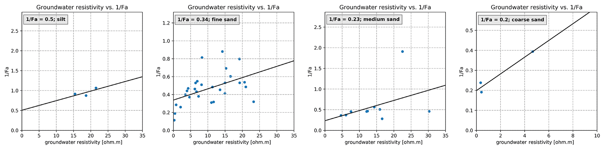
Figure B2 Relation between groundwater resistivity and $\mathrm{1}/F_{\text{a}}$ for four lithologies, from which F_i is obtained.

Appendix C: Drainable porosity

Average drainable porosity for aquifers in MKD is presented in Shrestha et al. (2016), based on a maximum of nine measurements per aquifer. It turned out that the data on drainable porosity are based on an unpublished mathematical transformation using horizontal hydraulic conductivity measurements, which are derived from pumping tests. The drainable porosity values (viz. 0.12–0.18) seem to be small with respect to the coarseness of the sediment, as described in the boreholes. Pechstein et al. (2018) present results of a pumping test in the Ca Mau province, with an average drainable porosity for the n22 aquifer of 0.22. Although this is only a single measurement, the drainable porosity seems to be more in line with what would be expected, given the coarseness of the sediments. To derive a spatially variable drainable porosity, borehole intervals were assigned drainable porosity values that depend on lithology. Values for lithology-dependent drainable porosity were derived from literature, especially Johnson (1967), which contains an in-depth analysis of drainable porosity for aquifers in the United States, based on the analysis of pumping tests in which the lithology of the aquifer was also described. The lithological description from Johnson (1967, table 29) is therefore linked to the lithology of the boreholes in the MKD and the corresponding drainable porosity assigned; see Table 1. To obtain a value of drainable porosity for each aquifer at borehole locations that is representative for the entire depth interval covering the aquifer, the weighted average of the drainable porosities of all the depth intervals that belong to the aquifer was calculated. Finally, depth-averaged drainable porosity maps per aquifer were obtained by interpolating between boreholes using ordinary kriging.

The results of the interpolation are depicted in Fig. C1. It turned out that the kriging variance (as a measure of the interpolation uncertainty) is small, with a coefficient of variation (CV) < 10 %. Therefore, the effect of interpolation uncertainty of the drainable porosity in the calculation of fresh groundwater volumes is discarded.

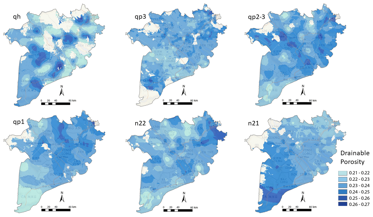
Figure C1 Maps of layer-average drainable porosity for aquifers in the MKD as obtained from ordinary kriging. In blank areas the aquifer is not present.

Appendix D: Hydrogeological model

For each unit, boreholes were selected that penetrate through that entire unit, and the base of the hydrogeological unit was determined. This new base was then compared to the base of the old, basic model of Minderhoud et al. (2017) at that location, and the residual (difference between the basic model and the base of the unit from the interpreted borehole) was interpolated using ordinary kriging. After adding the interpolated residual to the old basic model of Minderhoud et al. (2017), an updated and more detailed model of the base of each hydrogeological unit was obtained. The next step was to compare this updated model with the boreholes that did not penetrate the entire unit and, if necessary, to adjust the model. If the borehole that did not penetrate the entire hydrogeological unit encountered the new base of the updated model, the base of that unit in the borehole was assumed to be equal to the its current base plus an additional 5 m (the thickness of the voxel in the 3D model). The interpolation procedure was then repeated until the base of all non-penetrating boreholes complies with the interpolated base. Results are depicted in Fig. D1. The model of Minderhoud et al. (2017) was used for calculating land subsidence estimations and therefore did not include drainable porosity data and groundwater volumes were not determined.

Figure D1 Cross sections through the updated hydrogeological model. Scale according to kilometre reading along the axis (km) and depth in metres. Vertical exaggeration: 100×; aquifers (lower-case names) and aquitards (upper-case names).

Appendix E: Variogram analysis of TDS

To alleviate the burden of variogram inference (14 units, 11 indicators), the median indicator kriging approach was adopted, in which the semivariogram for the median of the distribution (TDS of 1 g L⁻¹ for all units) was used for all indicators. Research showed that there are only minor differences in interpolation results between full indicator kriging and median indicator kriging (Goovaerts, 2009). Experimental semivariograms and the semivariogram models for the median indicators of the declustered data are depicted in Fig. E1 for the six aquifers. From the experimental semivariograms it becomes clear that anisotropy in the horizontal plane is not apparent from the data: the experimental semivariograms for the northwest–southeast (N310) direction – the direction of flow of the fluvial system – are not fundamentally different from those in the direction perpendicular (N40). This indicates that the salinization of the (presumed) formerly fresh aquifers did occur independent from the (current) river flow direction.

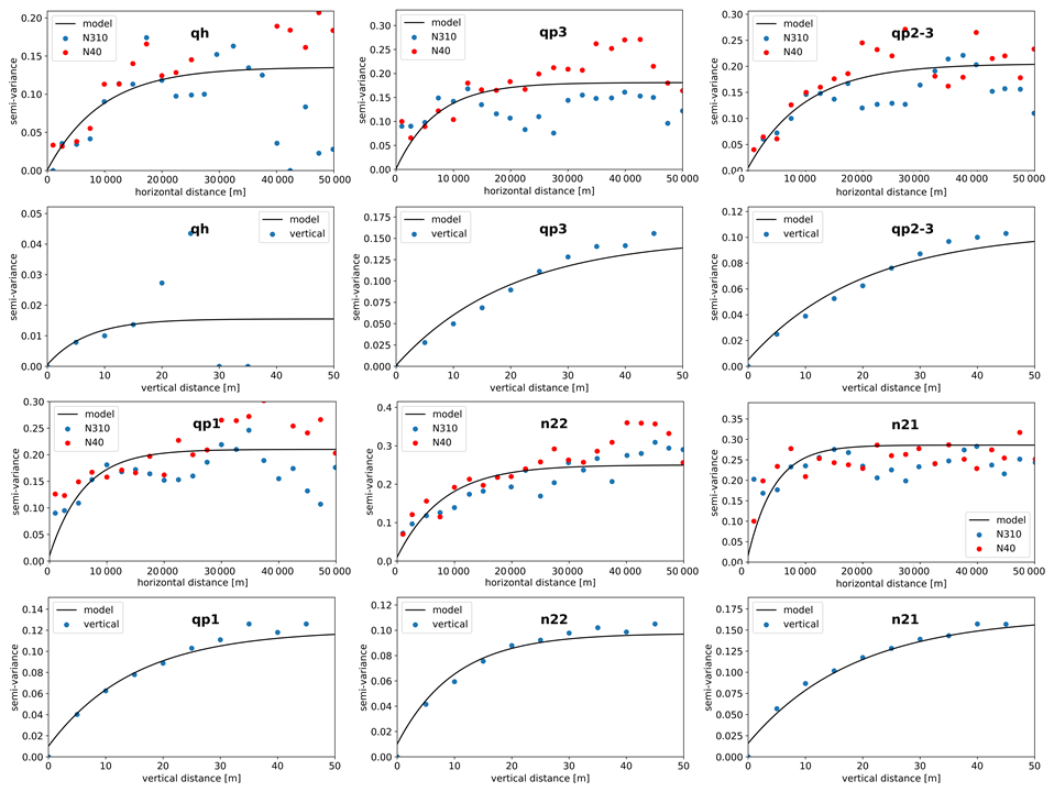
Figure E1 Horizontal and vertical experimental indicator semivariograms at indicator TDS = 1.0 g L⁻¹ and fitted exponential semivariogram models.

This confirms the concept of salinization of the groundwater as a consequence of widespread transgression during 12–2.5 ka before the present (Pham et al., 2019). The vertical semivariograms show spatial correlation distances up to tens of metres, indicating a strong continuity in TDS values in the vertical direction. The horizontal ranges of the semivariogram models are comparable to those found by Hoang (2008) for Pleistocene aquifers in Vietnam (Red River delta), which also showed almost no horizontal anisotropy. The minimum distance between the declustered data points is 1000 m in the horizontal direction. The variograms show a spatial correlation length that is larger than 1000 m, indicating that the horizontal voxel size is appropriate for the spatial scale considered.

Appendix F: Cross-validation of TDS

The cross-validation results for all aquifers are presented in Fig. F1. For a description of the graphs see Sect. 3.2.3 in the main text.

Figure F1 Results of the cross-validation per aquifer. Top left shows scatterplot of true versus E-type TDS estimate; top right indicates the accuracy of the interpolation by proportion of data that fall in a certain probability interval (PI); lower graph shows the summary of the cross-validation results concerning grouping of TDS values. For further explanation refer to the main text.