A daily, 250 m and real-time gross primary productivity product (2000–present) covering the contiguous United States

Gross primary productivity (GPP) quantifies the amount of carbon dioxide (CO₂) fixed by plants through photosynthesis. Although as a key quantity of terrestrial ecosystems, there is a lack of high-spatial-and-temporal-resolution, real-time and observation-based GPP products. To address this critical gap, here we leverage a state-of-the-art vegetation index, near-infrared reflectance of vegetation (NIR_V), along with accurate photosynthetically active radiation (PAR), to produce a SatelLite Only Photosynthesis Estimation (SLOPE) GPP product for the contiguous United States (CONUS). Compared to existing GPP products, the proposed SLOPE product is advanced in its spatial resolution (250 m versus >500 m), temporal resolution (daily versus 8 d), instantaneity (latency of 1 d versus >2 weeks) and quantitative uncertainty (on a per-pixel and daily basis versus no uncertainty information available). These characteristics are achieved because of several technical innovations employed in this study: (1) SLOPE couples machine learning models with MODIS atmosphere and land products to accurately estimate PAR. (2) SLOPE couples highly efficient and pragmatic gap-filling and filtering algorithms with surface reflectance acquired by both Terra and Aqua MODIS satellites to derive a soil-adjusted NIR_V (SANIR_V) dataset. (3) SLOPE couples a temporal pattern recognition approach with a long-term Cropland Data Layer (CDL) product to predict dynamic C4 crop fraction. Through developing a parsimonious model with only two slope parameters, the proposed SLOPE product explains 85 % of the spatial and temporal variations in GPP acquired from 49 AmeriFlux eddy-covariance sites (324 site years), with a root-mean-square error (RMSE) of 1.63 gC m⁻² d⁻¹. The median R² over C3 and C4 crop sites reaches 0.87 and 0.94, respectively, indicating great potentials for monitoring crops, in particular bioenergy crops, at the field level. With such a satisfactory performance and its distinct characteristics in spatiotemporal resolution and instantaneity, the proposed SLOPE GPP product is promising for biological and environmental research, carbon cycle research, and a broad range of real-time applications at the regional scale. The archived dataset is available at https://doi.org/10.3334/ORNLDAAC/1786 (download page: https://daac.ornl.gov/daacdata/cms/SLOPE_GPP_CONUS/data/, last access: 20 January 2021) (Jiang and Guan, 2020), and the real-time dataset is available upon request.

1 Introduction

Gross primary productivity (GPP) quantifies the amount of carbon dioxide (CO₂) fixed by plants through photosynthesis (Beer et al., 2010; Jung et al., 2017). Because GPP is the largest carbon flux and influences other ecosystem processes such as respiration and transpiration, monitoring GPP is crucial for understanding the global carbon budget and terrestrial-ecosystem dynamics (Bonan, 2019; Friedlingstein et al., 2019). In addition, biomass accumulation driven by GPP is the basis for food, feed, wood and fiber production, and therefore monitoring GPP is crucial for human welfare and development (Guan et al., 2016; Ryu et al., 2019).

Over the past 2 decades, a number of GPP products with different spatial and temporal characteristics have been derived using remote sensing approaches (Xiao et al., 2019). However, since GPP cannot be directly observed at large scales, different models have been developed and used in generating GPP products. Process-based models use a series of nonlinear equations to represent the atmosphere–vegetation–soil system and associated fluxes. For example, a publicly available global GPP product using process-based models is the Breathing Earth System Simulator (BESS) (Jiang and Ryu, 2016). Machine-learning models upscale site-observed GPP to a larger scale by establishing non-parametric relationships between the ground truth and gridded explanatory variables. The FLUXCOM GPP product is a typical example of this approach (Jung et al., 2019). Semi-empirical approaches utilize equations with a concise physiological meaning (e.g., light use efficiency) that are parameterized with several empirical constraint functions. The MOD17 (MODIS GPP/NPP – net primary production – Project) GPP product (Running et al., 2004), the Vegetation Photosynthesis Model (VPM) GPP product (Zhang et al., 2017) and the Global LAnd Surface Satellite (GLASS) GPP product (Yuan et al., 2010) belong to this category.

With differing principles, assumptions and complexity, existing remote sensing GPP models heavily rely upon inputs with large uncertainties. First, climate forcing, such as temperature, humidity, precipitation and wind speed, is commonly used in these GPP models. However, these meteorological data are not observed but derived from reanalysis approaches and usually have coarse spatial resolution (e.g., >10 km) and large time lags (e.g., weeks). Second, plant functional types (PFTs) are used to define different parameterization schemes in those models. To date, satellite land cover products are usually characterized by considerably large time lags (>1 year), relatively low accuracy (≤70 %) (Yang et al., 2017) and more uncertainties with regards to year-to-year variations (Cai et al., 2014; Li et al., 2018). Third, high-level remote sensing land products such as the leaf area index (LAI), fraction of absorbed photosynthetically active radiation (FPAR), clumping index (CI), land surface temperature (LST) and soil moisture (SM) are used by some models. These variables are not directly observed but retrieved by complicated algorithms, and their accuracy still needs significant improvement to meet requirements of Earth system models (GCOS, 2011).

Alternative approaches which heavily rely on reliable satellite observations with low dependence on uncertain model structure or parameterization and model inputs are highly required. Solar-induced fluorescence (SIF) emerged in recent years and may provide a new opportunity for GPP estimation (Guanter et al., 2014). Linear relationships have been found between SIF and GPP at various ecosystems (Liu et al., 2017; Magney et al., 2019; Yang et al., 2015). However, satellite SIF data generally have coarse resolution, large spatial gaps, short temporal coverage and limited quality (Bacour et al., 2019; Zhang et al., 2018) and are therefore not suitable for many applications.

Near-infrared reflectance of vegetation (NIR_V,Ref), defined as the product of the normalized difference vegetation index (NDVI) and observed NIR reflectance (NIR_Ref) (Eq. 1), has recently been presented as a proxy of GPP (Badgley et al., 2017). A global monthly 0.5^∘ GPP dataset has been produced from satellite data using the linear relationship between NIR_V,Ref and GPP (Badgley et al., 2019), explaining 68 % GPP variations observed by the FLUXNET network. Several field studies have recently found that taking incoming radiation into account further improves the NIR_V–GPP relationship (Dechant et al., 2020; Wu et al., 2020). Because MODIS provides long-term and real-time (2000–present) observations of red (Red_Ref) and NIR (NIR_Ref) reflectance and atmospheric conditions with high spatial (250 m for reflectance and 1 km for atmosphere) and temporal (daily) resolutions, now there is an unprecedented opportunity to generate an observation-based GPP product.

$$\begin{array}{}\text{(1)}& {\mathrm{NIR}}_{\mathrm{V},\mathrm{Ref}}=\mathrm{NDVI}\times {\mathrm{NIR}}_{\mathrm{Ref}}={\displaystyle \frac{{\mathrm{NIR}}_{\mathrm{Ref}}-{\mathrm{Red}}_{\mathrm{Ref}}}{{\mathrm{NIR}}_{\mathrm{Ref}}+{\mathrm{Red}}_{\mathrm{Ref}}}}\times {\mathrm{NIR}}_{\mathrm{Ref}}\end{array}$$

Leveraging the concept of NIR_V, here we present a new GPP model and the resultant daily, 250 m and real-time GPP product (2000–present) covering the contiguous United States (CONUS) (Jiang and Guan, 2020). The product is named SatelLite Only Photosynthesis Estimation (SLOPE) because (1) the model only uses satellite data and (2) the model only has two slope parameters. Detailed model design, multi-source satellite data processing and comprehensive evaluation procedures are elucidated below.

2 Production of the SLOPE product

The method we used to estimate GPP using the novel vegetation index NIR_V,Ref follows the concept of light use efficiency (LUE) (Monteith, 1972; Monteith and Moss, 1977):

$$\begin{array}{}\text{(2)}& \mathrm{GPP}=\mathrm{PAR}\times \mathrm{FPAR}\times \mathrm{LUE}.\end{array}$$

Since NIR_V,Ref has been found strongly correlated to FPAR (Badgley et al., 2017) and moderately correlated to LUE (Dechant et al., 2019), it is possible to simplify Eq. (2) as

$$\begin{array}{}\text{(3)}& \mathrm{GPP}\approx \mathrm{PAR}\times \left(a\times {\mathrm{NIR}}_{\mathrm{V},\mathrm{Ref}}+b\right),\end{array}$$

where a and b are the slope and intercept, which can be fitted from ground GPP observations. Both PAR (photosynthetically active radiation) and NIR_V,Ref can be easily derived from satellite observations with high spatial and temporal resolutions in real time, avoiding complicated but uncertain algorithm or parameterization to quantify FPAR and LUE in Eq. (2). This linear relationship is likely to converge within C3 species (Badgley et al., 2019) but differs between C3 and C4 species (Wu et al., 2019). Accordingly, land cover data with considerably large time lags and relatively low accuracy may not be necessary for the model parameterization. Instead, an in-season C3–C4 species dataset is needed for the accurate calibration of the linear relationship.

Defining the ratio of GPP to PAR as the incident PAR use efficiency (iPUE) gives

$$\begin{array}{}\text{(4)}& \mathrm{iPUE}=\mathrm{GPP}/\mathrm{PAR}=\mathrm{FPAR}\times \mathrm{LUE}\approx a\times {\mathrm{NIR}}_{\mathrm{V},\mathrm{Ref}}+b.\end{array}$$

Here iPUE is a confounding factor of canopy structure and leaf physiology, representing the capacity of plants to use incoming radiation for photosynthesis. When vegetation is absent, iPUE is zero and NIR_V,Ref is expected to be zero too. However, this is not true in reality, as >99.9 % soils have positive NIR_V,Ref values according to a global soil spectral library (Jiang and Fang, 2019), and the correction of NIR_V,Ref for soil is needed for better performance at low vegetation cover (Zeng et al., 2019). To address this issue, we will propose a spatially explicit correction for NIR_V,Ref to derive a soil-adjusted index SANIR_V (see details in Sect. 2.2). Since SANIR_V=0 when iPUE = 0, Eq. (4) becomes

$$\begin{array}{}\text{(5)}& \mathrm{iPUE}\approx c\times {\mathrm{SANIR}}_{\mathrm{V}},\end{array}$$

where c is the slope coefficient.

Considering the presence of mixed pixels of C3 and C4 species with the 250 m pixels, Eq. (5) can be rewritten as

$$\begin{array}{}\text{(6)}& \mathrm{iPUE}\approx \left[c_{\mathrm{C}\mathrm{4}}\times f_{\mathrm{C}\mathrm{4}}+c_{\mathrm{C}\mathrm{3}}\times \left(\mathrm{1}-f_{\mathrm{C}\mathrm{4}}\right)\right]\times {\mathrm{SANIR}}_{\mathrm{V}},\end{array}$$

where c_C4 and c_C3 are the coefficients for C4 and C3 species, respectively, and f_C4 is the fraction of C4 species in vegetation. Therefore, the SLOPE GPP model is

$$\begin{array}{}\text{(7)}& \mathrm{GPP}\approx \left[c_{\mathrm{C}\mathrm{4}}\times f_{\mathrm{C}\mathrm{4}}+c_{\mathrm{C}\mathrm{3}}\times \left(\mathrm{1}-f_{\mathrm{C}\mathrm{4}}\right)\right]\times \mathrm{PAR}\times {\mathrm{SANIR}}_{\mathrm{V}}.\end{array}$$

In the SLOPE model (Eq. 7), PAR, SANIR_V and f_C4 are remote sensing inputs, whereas c_C4 and c_C3 are model parameters to be calibrated using ground-truth GPP data (Fig. 1). In the following sections, we will elaborate on the derivation of PAR, SANIR_V and f_C4, along with their quantitative uncertainties, and the model calibration for parameters c_C4 and c_C3. With the uncertainty of each term (Δc_C4, Δc_C3, Δf_C4, ΔPAR and ΔSANIR_V), the uncertainty of GPP can be estimated in a spatiotemporally explicit manner by

$$\begin{array}{}\text{(8)}& \begin{array}{rl}\mathrm{\Delta }\mathrm{GPP}& =\left(f_{\mathrm{C}\mathrm{4}}\times \mathrm{PAR}\times {\mathrm{SANIR}}_{\mathrm{V}}\right)\times \mathrm{\Delta }{c}_{\mathrm{C}\mathrm{4}}\\ & +\left[\left(\mathrm{1}-f_{\mathrm{C}\mathrm{4}}\right)\times \mathrm{PAR}\times {\mathrm{SANIR}}_{\mathrm{V}}\right]\mathrm{\Delta }{c}_{\mathrm{C}\mathrm{3}}\\ & +\left[\left(c_{\mathrm{C}\mathrm{4}}-c_{\mathrm{C}\mathrm{3}}\right)\times \mathrm{PAR}\times {\mathrm{SANIR}}_{\mathrm{V}}\right]\mathrm{\Delta }{f}_{\mathrm{C}\mathrm{4}}\\ & +\left\{\left[c_{\mathrm{C}\mathrm{4}}\times f_{\mathrm{C}\mathrm{4}}+c_{\mathrm{C}\mathrm{3}}\times \left(\mathrm{1}-f_{\mathrm{C}\mathrm{4}}\right)\right]\times {\mathrm{SANIR}}_{\mathrm{V}}\right\}\mathrm{\Delta }\mathrm{PAR}\\ & +\left\{\left[c_{\mathrm{C}\mathrm{4}}\times f_{\mathrm{C}\mathrm{4}}+c_{\mathrm{C}\mathrm{3}}\times \left(\mathrm{1}-f_{\mathrm{C}\mathrm{4}}\right)\right]\times \mathrm{PAR}\right\}\mathrm{\Delta }{\mathrm{SANIR}}_{\mathrm{V}}\end{array}.\end{array}$$

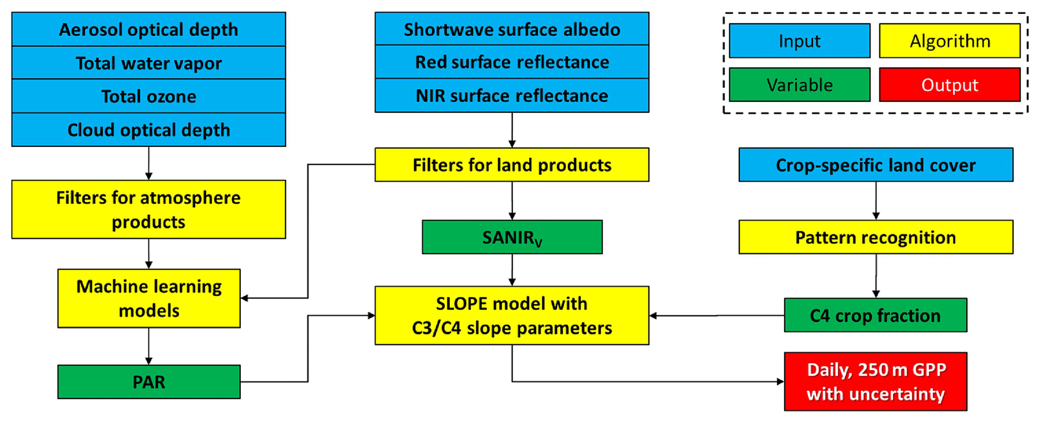
Figure 1 Framework to produce the SLOPE GPP product. The box with dashed lines is the legend.

2.1 Derivation of PAR

SLOPE adopts several machine learning approaches to compute PAR using forcing data mainly from Terra and Aqua MODIS Atmosphere and Land products (data solely from morning satellite Terra, afternoon satellite Aqua and combination of the two satellites are called MOD, MYD and MCD, respectively, hereinafter). The list of inputs includes aerosol optical depth (AOD) at 3 km resolution from the MOD04_3K (MODIS/Terra Aerosol 5Min L2 Swath 3km) and MYD04_3K (MODIS/Aqua Aerosol 5Min L2 Swath 3km) products (Remer et al., 2013), total column water vapor (TWV) at 1 km resolution from the MOD05_L2 (MODIS/Terra Total Precipitable Water Vapor 5-Min L2 Swath 1km and 5km) and MYD05_L2 (MODIS/Aqua Total Precipitable Water Vapor 5-Min L2 Swath 1km and 5km) products (Chang et al., 2015), cloud optical thickness (COT) at 1 km resolution from the MOD06_L2 (MODIS/Terra Clouds 5-Min L2 Swath 1km and 5km) and MYD06_L2 (MODIS/Aqua Clouds 5-Min L2 Swath 1km and 5km) products (Baum et al., 2012), total column ozone burden (TO3) at 5 km resolution from the MOD07_L2 (MODIS/Terra Temperature and Water Vapor Profiles 5-Min L2 Swath 5km) and MYD07_L2 (MODIS/Aqua Temperature and Water Vapor Profiles 5-Min L2 Swath 5km) products (Borbas et al., 2015), white-sky land surface shortwave albedo (ALB) at 500 m resolution from the MCD43A3 (MODIS/Terra+Aqua Albedo Daily L3 Global 500m SIN Grid) product (Román et al., 2009), and altitude (ALT) at 30 m resolution from the Shuttle Radar Topography Mission Global 1 arc second (SRTMGL1) product (Kobrick and Crippen, 2017).

MODIS atmosphere products are swath data, and swaths vary day by day. To maintain consistency and facilitate further usage, all data are reprojected using the nearest neighbor resampling approach to the Conus Albers projection on the North American Datum of 1983 (NAD83) (European Petroleum Survey Group – EPSG:6350) with 1 km spatial resolution. For swath data, an overlap area exists between two paths. In this case, data with smaller sensor view zenith angles provided by MOD/MYD03_L2 products are chosen. MODIS land products and SRTMGL1 are tile data with finer resolution than 1 km. They are reprojected to the EPSG 6350 spatial reference by aggregating all fine-resolution pixels within each 1 km grid.

Data gaps exist in all MODIS products, and a gap-filling measure is required. For MODIS atmosphere products, gaps in MOD and MYD are first filled by data in the MYD and MOD counterpart on the same day, followed by a multi-year average on that day. Since the multi-year average of COT is always non-zero, directly using it for a gap-filling measure always implies a cloudy condition. Therefore, a CLARA-2 (cLoud, Albedo and surface Radiation) cloud mask at 0.05^∘ acquired from NOAA AVHRR (Advanced Very High Resolution Radiometer) data is employed (Karlsson et al., 2017). Only MODIS data gaps for AVHRR cloudy pixels are filled by a multi-year average of COT, whereas MODIS COT data gaps for AVHRR clear pixels are set to 0. For the MODIS land product, i.e., ALB, a temporally moving window with a 7 d radius is utilized for a specific day, and a Gaussian filter is applied to the time series data within the moving window on a per-pixel basis. The filtered values are used to fill gaps on that specific day.

Machine learning approaches are used to upscale the ground truth to satellite data. The ground truth is from the Surface Radiation Budget (SURFRAD) Network (Augustine et al., 2000), including seven long-term continuous sites across the CONUS. Daily-mean shortwave radiation (SWR) and PAR on the surface are calculated from site observations at 1–3 min intervals from 2000 through 2018. Daily-mean top-of-atmosphere SWR (SWR_TOA) is calculated using latitude and day-of-year (DOY) information (Allen et al., 1998). Subsequently, atmospheric transmittance (t_SWR) and proportion of PAR in SW (p_PAR) are calculated as SWR $/$ SWR_TOA and PAR $/$ SWR.

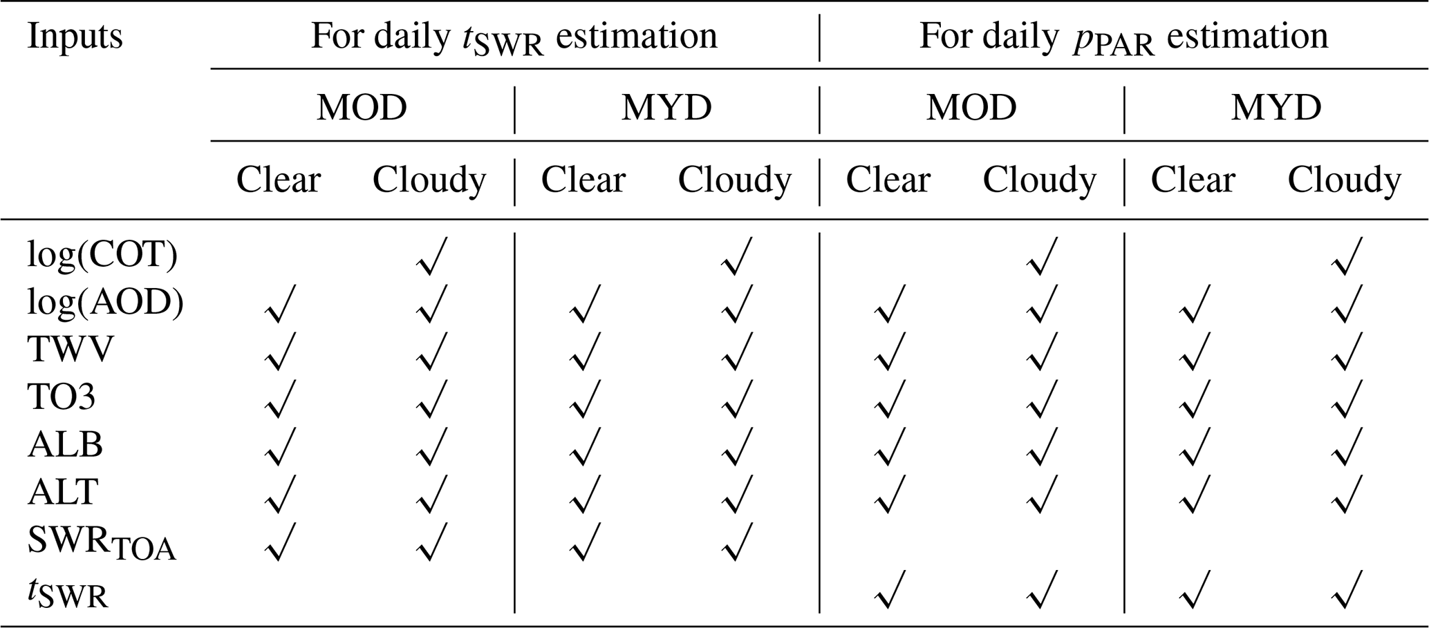
Models are built to estimate t_SWR first, followed by p_PAR. MOD data representing atmospheric conditions in the morning and MYD for the afternoon are used separately for the estimation, and the two estimates are averaged to account for discrepancies between the morning and afternoon. Clear and cloudy conditions are also treated separately in modeling considering the absence or presence of non-zero COT data. For the estimation of t_SWR, ALB, ALT and SWR_TOA are used in addition to atmosphere data, whereas for p_PAR, ALB, ALT and the estimated t_SWR are used. A summary of model inputs is listed in Table 1.

Table 1 Summary of machine learning model inputs for the estimation of t_SWR and p_PAR. Daily estimations from MOD and MYD atmosphere data are averaged.

Four different machine learning approaches are employed to estimate t_SWR and p_PAR. They are the least absolute shrinkage and selection operator (LASSO) (Tibshirani, 1996), multivariate adaptive regression splines (MARS) (Friedman, 1991), k-nearest neighbor regression (KNN) (Goldberger et al., 2005), and random forest regression (RF) (Liaw and Wiener, 2002). We used scikit-learn, a free software machine learning library for the Python programming language to build the models. All the four algorithms were automatically optimized by tuning their hyperparameters using 5-fold cross validation on their training dataset. All inputs and outputs are the same for the four approaches. Four different PAR estimations are then obtained by Eq. (9), and their ensemble mean and standard deviation are considered as the final estimation and uncertainty, respectively.

$$\begin{array}{}\text{(9)}& \mathrm{PAR}={\mathrm{SWR}}_{\mathrm{TOA}}\times t_{\mathrm{SWR}}\times p_{\mathrm{PAR}}\end{array}$$

2.2 Derivation of SANIR_V

SLOPE derives NIR_V,Ref (Eq. 1) from MODIS band 1 (red) and band 2 (NIR) surface reflectance (SR) at 250 m resolution from MOD/MYD09GQ products (Vermote et al., 2002). Only pixels with quality control (QC) information defined as “corrected product produced at ideal quality all bands” were used. Since cloud and cloud shadows substantially reduce NIR_V,Ref values, SLOPE adopts three strategies to mitigate the cloud contamination.

First, the cloud mask is applied. MOD–MYD COT data processed in Sect. 2.1 are resampled to the same spatial reference with MOD–MYD SR data and used to mask out cloudy pixels. At this point, a morphological dilation operation is used to enlarge the cloud mask to account for cloud edges. However, since COT data have a coarser resolution (1 km) than SR data (250 m), there are still partial clouds and cloud shadows left after this step.

Second, MOD and MYD data are combined. Ideally, on a specific day, MOD and MYD NIR_V,Ref should be identical if they are obtained under the same conditions. However, the remaining cloud contamination and sun-target-sensor geometry could cause differences between morning and afternoon observations. Considering that the vegetation index is more sensitive to cloud contamination than the sensor view zenith angle, a simple criterion is applied to combine MOD and MYD observations. If the difference between MOD and MYD NIR_V,Ref is greater than or equal to a predefined threshold (0.1 in this study), then the smaller one is likely cloud contaminated, and the larger one is used. Otherwise, the average value of the two is used. However, in many cases, both MOD and MYD data are contaminated, and the sensor view zenith angle may cause unexpected day-to-day variations.

Third, a temporal filter is applied. The filter is based on the assumption that NIR_V,Ref should change smoothly within a short time period. Accordingly, a temporally moving window with a 7 d radius is utilized for a specific day. The mean and standard deviation are calculated from the NIR_V,Ref time series on a per-pixel basis. Values outside the range of mean ±1.5 standard deviations are considered as outliers and dropped. Subsequently, the mean of the first 3 d and that of the last 7 d are calculated, respectively. If the NIR_V,Ref value of the target day is 20 % smaller or larger than both the first 3 d mean and the last 3 d mean, then that NIR_V,Ref value is considered as an outlier and dropped.

After the removal of outliers, a large amount of data gaps exist, and a gap-filling measure is required. Similar to ALB in Sect. 2.1, a temporally moving window with a 7 d radius is utilized for a specific day, and a Gaussian filter is applied and used to fill gaps on that day. The rest of the data gaps are filled with the multi-year average of NIR_V,Ref. Considering extreme cases for which no data are available on a specific day over all years, the multi-year average of ±3 d is used for the final gap-filling measure.

To minimize the effects of variations in soil brightness on NIR_V,Ref, soil background NIR_V (NIR_V,Soil) is identified from multi-year average NIR_V,Ref time series. For a specific pixel, soil background NIR_V (NIR_V,Soil) is supposed to be (1) smaller than seasonal mean NIR_V,Ref, which includes the vegetated period, and (2) smaller than 0.2 indicated by a global soil spectral library (Jiang and Fang, 2019). Therefore, NIR_V,Soil is supposed to within a range of [0, min(mean(NIR_V,Ref), 0.2)]. The mode of daily NIR_V,Ref averaged over 2000–2019 within this value range is considered as NIR_V,Soil. An example is given in Fig. S5. Theoretically, NIR_V,Soil for evergreen species cannot be obtained from time series NIR_V,Ref because of the persistent vegetation cover. Pixels with a NIR_V,Soil value larger than 0.1 and seasonal coefficient of variation (CV) of NIR_V,Ref smaller than 33 % are empirically considered as evergreen species, and their NIR_V,Soil values are set to 0.

Finally, SANIR_V is defined as

$$\begin{array}{}\text{(10)}& {\mathrm{SANIR}}_{\mathrm{V}}={\displaystyle \frac{{\mathrm{NIR}}_{\mathrm{V},\mathrm{Ref}}-{\mathrm{NIR}}_{\mathrm{V},\mathrm{Soil}}}{{\mathrm{NIR}}_{\mathrm{V},\mathrm{Peak}}-{\mathrm{NIR}}_{\mathrm{V},\mathrm{Soil}}}}\times {\mathrm{NIR}}_{\mathrm{V},\mathrm{Peak}},\end{array}$$

where NIR_V,Peak is the maximum value of the multi-year average NIR_V,Ref time series on a per-pixel basis. SANIR_V does not change NIR_V,Peak but changes more for low NIR_V,Ref values. SANIR_V,Ref is set to 0 when NIR${}_{\mathrm{V},\mathrm{Ref}}\le$ NIR_V,Soil. In general, SANIR_V is supposed to be smooth within a short time period; therefore, the standard deviation within the ±3 d temporal window is calculated as uncertainty.

2.3 Derivation of the C4 fraction

A National Land Cover Database (NLCD) along with a crop-specific land cover product Cropland Data Layer (CDL) are used to derive the fraction cover of C4 crop in vegetation (f_C4). NLCD is a comprehensive land cover database produced by the United States Geological Survey (USGS). It provides several main thematic classes such as urban, agriculture and forest with high accuracy (Homer et al., 2004). The 30 m nationwide NLCD data are available for 2001, 2004, 2006, 2008, 2011, 2013 and 2016. CDL is an agriculture-oriented product produced by the United States Department of Agriculture (USDA). It provides >100 crop cover types and leverages other land cover types from NLCD (Boryan et al., 2011). Across the CONUS CDL data are available at a 30 m spatial resolution and in a yearly temporal frequency from 2008 through 2019, whereas in some areas annual data are available back to the 1990s.

The fraction of C4 crop in vegetated areas is first derived using existing CDL data. NLCD land cover types are categorized into vegetated areas and non-vegetated areas with 30 m resolution. The fraction of vegetated areas in total area is subsequently calculated for each 250 m pixel. Similarly, CDL crop types are categorized into C4-planted areas and non-C4 areas with 30 m resolution. The fraction of C4 crops in total area is subsequently calculated for each 250 m pixel. The ratio of the fraction of C4 crops in total area to the fraction of vegetated areas in total area is calculated to derive the fraction of C4 crops in vegetated areas at 250 m resolution. Since NLCD data are not available for every year, an assumption is made that 1 year of NLCD data can represent adjacent years. Specifically, NLCD 2001 is used for 2000–2002; NLCD 2004 is used for 2003 and 2004; NLCD 2006 is used for 2005 and 2006; NLCD 2008 is used for 2007–2009; NLCD 2011 is used for 2010 and 2011; NLCD 2013 is used for 2012–2014; and NLCD 2016 is used for 2015–2019.

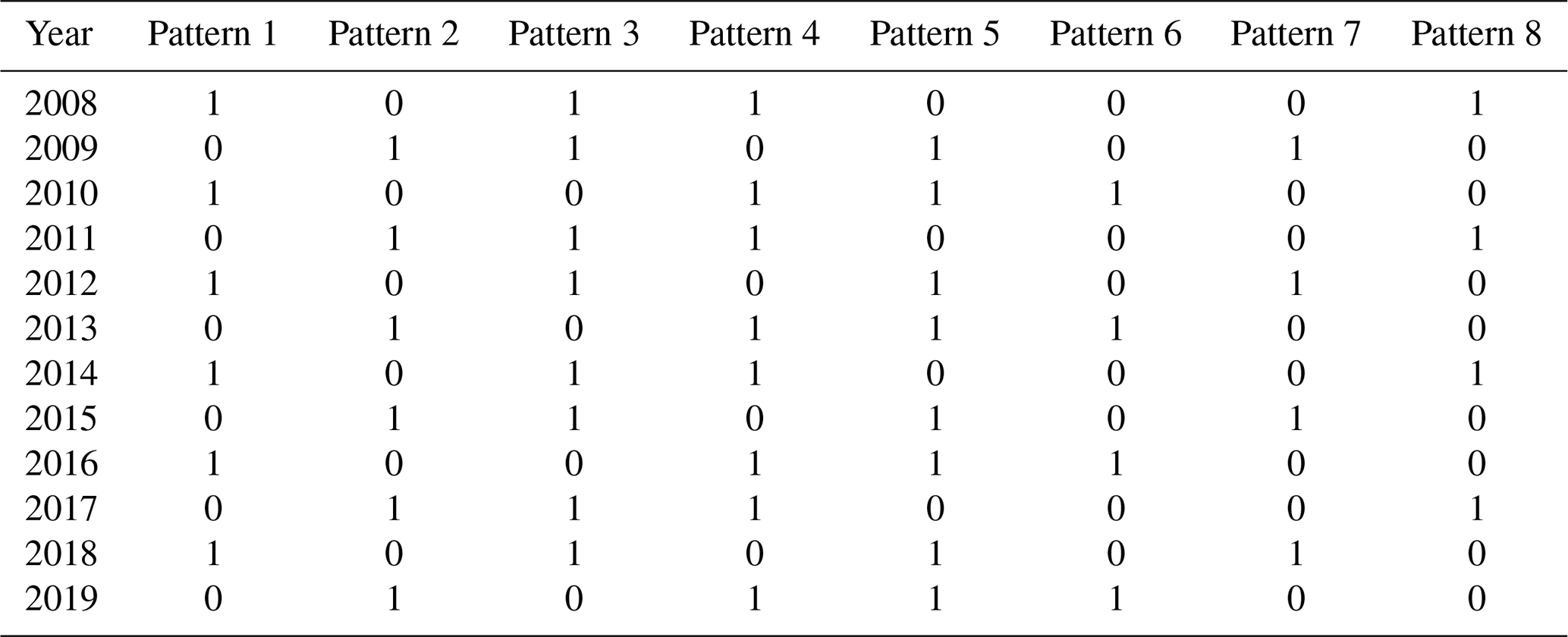
To predict the fraction of C4 crop in vegetation for region years for which no CDL data are available, crop rotation patterns are identified from historical data. Assuming that C4 crops are planted following three rotation strategies: C4–non-C4, C4–C4–non-C4 and non-C4–non-C4–C4 and assigning 1 to C4 and 0 to non-C4, a total of eight possible time series during the period of 2008–2019 when nationwide CDL data are available are listed in Table 2. On a per-pixel basis, the time series of the fraction of C4 crop in vegetation areas during 2008–2019 is compared with the eight predefined rotation patterns. The Pearson coefficient r is calculated between actual time series and each of the eight patterns, and the pattern yielding the largest r is the identified rotation pattern. Once the pattern is identified, the fraction of C4 crop in vegetated areas in any unknown year can be inferred. If 1 year is inferred as C4, then the multi-year average of the C4 fraction over C4-dominated years is used. Otherwise, the multi-year average over C3-dominated years is used. If the largest r is smaller than 0.497, i.e., p>0.1 for 12 years, then it is considered as no significant pattern, and the multi-year average over all years is used. The RMSE between the predicted and reference CDL C4 fraction is calculated as uncertainty. To account for the land cover change, the predicted C4 crop fraction is set to 0 in years when NLCD data are not classified as cropland. It is worth mentioning that C4 grassland and shrubland are not considered in this study, as no nationwide high-resolution distribution data are available.

Table 2 Predefined C4-planting patterns from 2008 through 2019. If the C4 crop dominates in a specific year, 1 is assigned. Otherwise, 0 is assigned.

2.4 Calibration for iPUE coefficients

SLOPE was calibrated using the GPP data derived from AmeriFlux site observations. The AmeriFlux network is a community of sites that use eddy-covariance technology to measure landscape-level carbon, water and energy fluxes across the Americas (Baldocchi et al., 2001). A total of 48 sites (324 site years) were involved in this study (Table S3). All of the 43 sites in the FLUXNET2015 Tier 1 dataset (variable name: GPP_DT_VUT_MEAN; quality control: NEE_VUT_REF_QC) in the CONUS were used because this dataset was produced by a standardized data processing pipeline with strict data quality control protocols and is commonly considered the ground truth. Additionally, seven sites were from the AmeriFlux level 4 dataset (variable name: GPP_or_MDS; quality control: NEE_or_fMDSsqc). This dataset was generated more than 10 years ago, and only AmeriFlux Core Sites that are not covered by FLUXNET2015 were used for data quality consideration. For both datasets, only days with the best quality control flags were used in the SLOPE modeling and evaluation procedures.

We used Eq. (5) to conduct model calibration. Although SLOPE considers the iPUE–SANIR_V relationship for C3 and C4 species, we also tested other configurations for comparison purposes. Configuration 1 (“all”) is defined as follows: all data were used together to fit a universal iPUE coefficient c. Configuration 2 (“C3–C4”) is defined as follows: data were separated for C3 and C4 species to fit c_C3 and c_C4, respectively. It is worth mentioning that only C4 crops (six sites) were considered as C4 species, whereas C4 grass and shrubs (three sites: US-SRG, Santa Rita Grassland; US-SRM, Santa Rita Mesquite; and US-Wkg, Walnut Gulch Kendall Grasslands) were still categorized into C3 species because of the lack of nationwide and high-resolution C4 grass and shrub data. Configuration 3 (“PFTs”) is defined as follows: data were separated for different PFTs, evergreen needleleaf forest (ENF; 14 sites), deciduous broadleaf forest and mixed forest (DBF and MF; 8 sites), shrubland and woody savannah (SHR and WSA; 5 sites), grassland (GRA; 8 sites), wetland (WET; 5 sites), C3 cropland (10 sites) and C4 cropland (6 sites), to fit PFT-specific iPUE coefficients. The RMSE between SANIR_V-derived and AmeriFlux iPUE for C3 and C4 are calculated as uncertainties of c_C3 and c_C4, respectively.

3 Evaluation of the SLOPE product

3.1 Performance of PAR

SLOPE PAR demonstrates distinctive and detailed spatial variations in the CONUS because of the large spatial variations of atmospheric conditions (Fig. 2a). As an example, on 10 July 2020, large areas in New Jersey, Wisconsin, Oklahoma, South Dakota and Montana display significantly lower values than other areas, due to dominant impacts of clouds (Fig. S1). Aerosol optical depth (Fig. S2), total water vapor (Fig. S3) and total ozone burden (Fig. S4) also influence the amount of clear-sky PAR to some degree. For example, the southeastern part of the CONUS shows more aerosol and thus lower PAR values than other cloud-free areas. In addition to the total amount of PAR, SLOPE PAR also reveals variations in the ratio of PAR to SWR (Fig. S5). Despite a relatively small range (0.40–0.46), it is negatively correlated with cloud optical thickness and total ozone burden and positively correlates with total water vapor. PAR uncertainties caused by the difference of the four machine learning algorithms are generally small (<5 %; Fig. 2b). Higher uncertainties are mainly distributed in cloudy and desert areas.

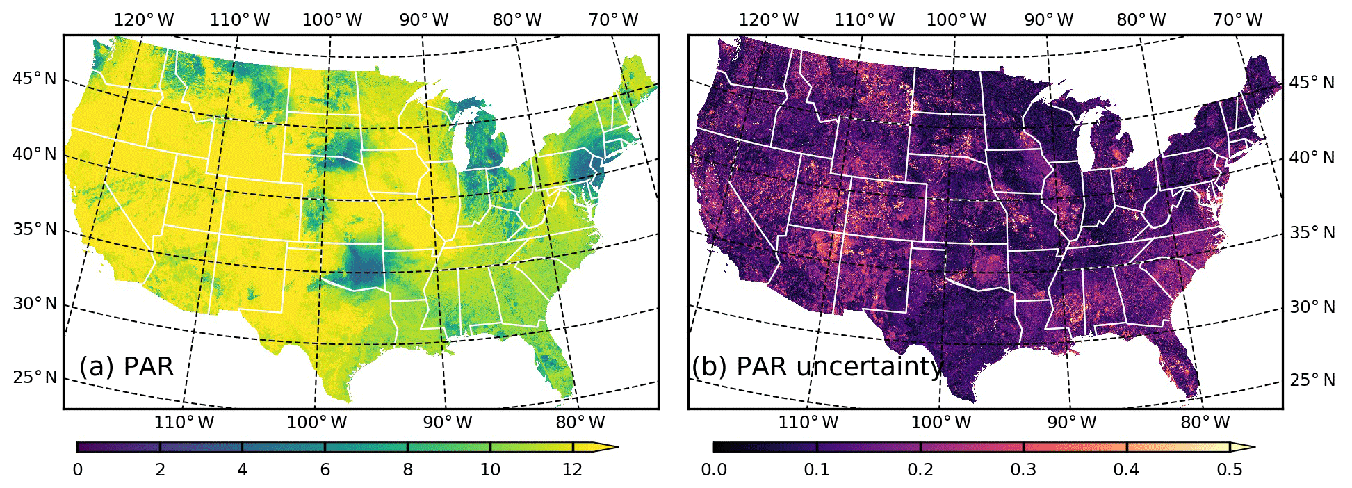
Figure 2 Spatial distribution of 1 km resolution (a) PAR (MJ m⁻² d⁻¹) and (b) PAR uncertainty (MJ m⁻² d⁻¹) on 10 July 2020.

To evaluate SLOPE PAR, we used two different site observation datasets which are independent of the PAR derivation procedure. The first dataset is SURFRAD (Table S1). While SURFRAD data from 2000 through 2018 were used for model training, we used data in 2019 for evaluation. The second dataset is FLUXNET2015 (Table S2). A total of 41 sites providing PAR data were used for the evaluation. For both datasets, only days with the best quality control flags were used.

Evaluation results show that SLOPE PAR is in a highly aligned agreement with the ground truth independent from the training procedure (Fig. 3). Across the seven SURFRAD sites in 2019 and the 41 AmeriFlux sites from 2000 to 2014, SLOPE PAR achieves an overall coefficient of determination (R²) of 0.91 and root-mean-square error (RMSE) values of 1.09 and 1.19 MJ m⁻² d⁻¹, respectively. In addition, the performance is reasonably stable under different sky conditions, indicated by similar R² and RMSE values from low to high atmospheric transmittance (Fig. S6).

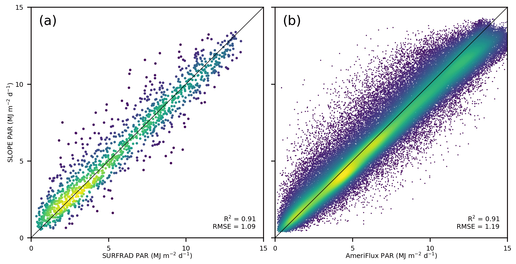
Figure 3 Comparison between site-observed PAR and SLOPE PAR. (a) Comparison across seven SURFRAD sites in 2019. (b) Comparison across 41 AmeriFlux sites from 2000 to 2014. All site data are independent of the training procedure.

3.2 Performance of SANIR_V

SLOPE SANIR_V demonstrates detailed and distinctive spatial variations in the CONUS (Fig. 4a). In the peak growing season, remarkably high SANIR_V values (∼ 0.5) from the Corn Belt in the central US are observed. This area is one of the most productive areas on Earth, producing more than 30 % of global corn and soybean (Green et al., 2018). Forested areas in the eastern and western US are characterized by relatively high values (0.3–0.4) and medium values (0.2–0.3), respectively. Low values (<0.2) are mainly observed in grasslands and shrublands in the western US. Uncertainty is associated with SANIR_V data on the pixel basis (Fig. 4b). In general, areas with higher SANIR_V values also have higher uncertainties. However, this pattern is altered by atmospheric conditions, where areas with higher cloud optical thickness (Fig. S1), aerosol optical depth (Fig. S2) and water vapor (Fig. S3) values tend to have larger uncertainties.

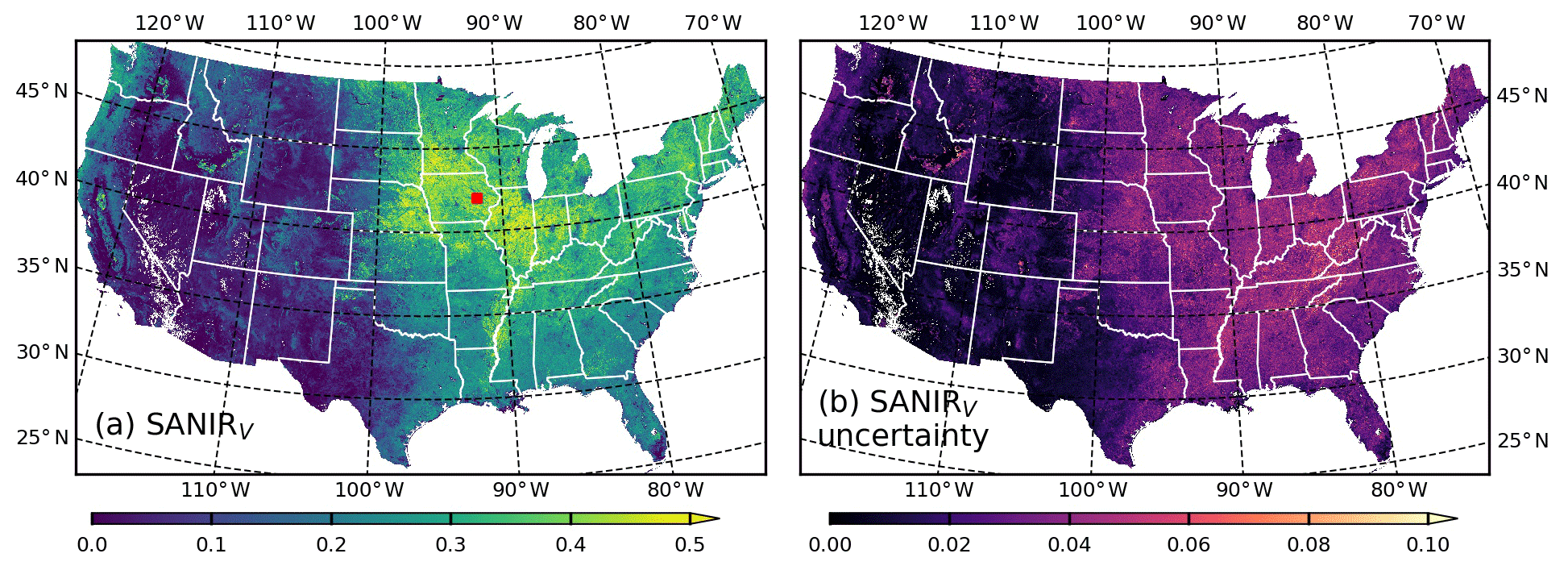
Figure 4 Spatial distribution of 250 m resolution (a) SANIR_V and (b) SANIR_V uncertainty across the CONUS on 10 July 2020.

Figure 5 demonstrates that SLOPE SANIR_V is able to capture spatial and temporal variations at a small scale (e.g., within a county). An overall drop in SANIR_V due to an extreme event damage can be observed within a short time period, thanks to the high temporal resolution (daily) of the SLOPE product. In addition, differences between plots possibly indicating different varieties, planting density and management can also be observed, thanks to the high spatial resolution (250 m) of the SLOPE product.

Figure 5 SANIR_V in a 50×75 km² area at Cedar Rapids, Iowa (red marker in Fig. 4a), on (a) 9 Aug 2020 and (b) 13 Aug 2020. A severe derecho took place from 10–11 August 2020. The maps are shown with the sinusoidal projection.

SLOPE SANIR_V shows significantly different seasonality for different PFTs (Fig. 6). The evergreen needleleaf forest site US-Blo (Blodgett Forest) is characterized by a relatively stable SANIR_V seasonal cycle in 2019 (Fig. 6a), indicated by a CV of 14.9 % only. The deciduous broadleaf forest site US-Ha1 (Harvard Forest EMS Tower) has a large seasonal variation with a CV of 108.6 % (Fig. 6b). The SANIR_V value suddenly rises from 0 to 0.3 in May, reaches 0.4 in June and July and gradually decreases back to 0 in October. The hot desert open shrubland site US-Whs (Walnut Gulch Lucky Hills Shrub) has an overall low SANIR_V value (Fig. 6c), with a peak value observed in early October. The grassland site US-AR1 (ARM USDA UNL OSU Woodward Switchgrass 1) shows a distinct double-peak (in June and September) seasonal pattern (Fig. 6d), which is caused by the precipitation seasonality there. The wetland site US-Myb (Mayberry Wetland) is characterized by a long growing season and a flat peak from April to November (Fig. 6e). The cropland site US-Bo1 (Bondville) has corn planted in 2019, and it shows the highest SANIR_V peak up to 0.5 among all the shown six sites (Fig. 6f). It is worth mentioning that compared to the two raw satellite-observed NIR_V values provided by MOD09GQ and MYD09GQ products, respectively, SLOPE SANIR_V successfully removes the soil impact in the non-growing season as the values equal to or close to 0. In addition, SLOPE SANIR_V is gap-free and much less contaminated by noises. Furthermore, spatiotemporally explicit uncertainty is associated with each SANIR_V value.

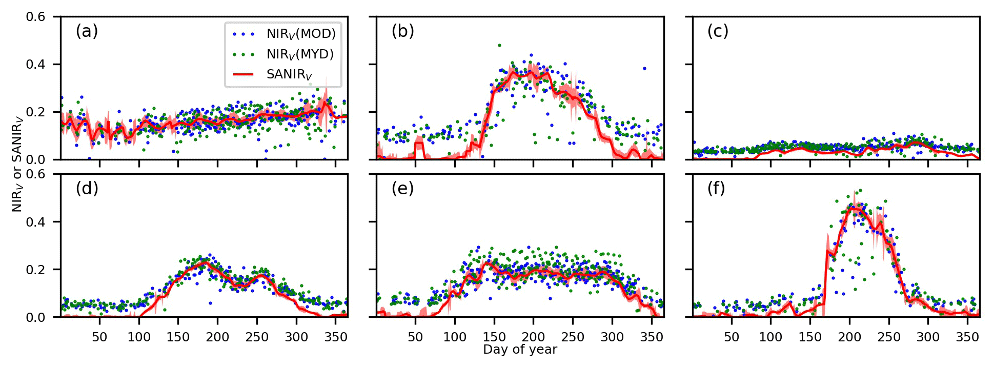
Figure 6 Comparison between SANIR_V and raw NIR_V derived from MOD09GQ and MYD09GQ products at six AmeriFlux sites (Table S3) in 2019. (a) US-Blo (evergreen needleleaf forest, ENF). (b) US-Ha1 (deciduous broadleaf forest, DBF). (c) US-Whs (open shrubland, OSH). (d) US-AR1 (grassland, GRA). (e) US-Myb (wetland, WET). (f) US-Bo1 (cropland, CRO). Shaded areas indicate uncertainties of SANIR_V.

3.3 Performance of the C4 fraction

SLOPE predicts a reasonable fraction of the C4 crop in vegetation in the CONUS (Fig. 7a). Most of the C4 crops are located in the Corn Belt, especially in Indiana, Illinois, Iowa and Nebraska. A direct comparison between the predicted C4 crop fraction (Fig. 8a) and independent reference CDL data (Fig. 8b) indicates that the SLOPE prediction is able to reconstruct the spatial patterns of the fraction of C4 crop in vegetation at 250 m resolution. It is worth mentioning that the uncertainty metric RMSE is sensitive to extreme values, and it is different from the misclassification rate (0.4 does not mean 40 %). For a pure pixel of a corn–soybean rotation field, the RMSE equals 0.39 if 3 out of 20 years are misclassified, i.e., misclassification rate of 0.15. A further investigation with regard to interannual dynamics shows that the SLOPE predictions can even perform better than CDL reference data (Fig. 9), benchmarked with the ground truth collected in the field. At this point, the CDL land cover could be prone to uncertainties in both satellite observation and classification algorithm, and classification is conducted year by year without an interannual consideration (Lark et al., 2017). SLOPE employs a rotation model to match decadal time series of CDL data, during which procedure noises in CDL data are suppressed. The features for which SLOPE is able to reconstruct spatial and interannual patterns of CDL data enable producing GPP in years when CDL data are unavailable (e.g., 2020 and years before 2008 for most regions). It is worth mentioning that uncertainty is also associated with each pixel (Fig. 7b).

Figure 7 Spatial distribution of 250 m resolution (a) predicted fraction of C4 crop in vegetation in 2000 and (b) C4 crop fraction uncertainty across the CONUS.

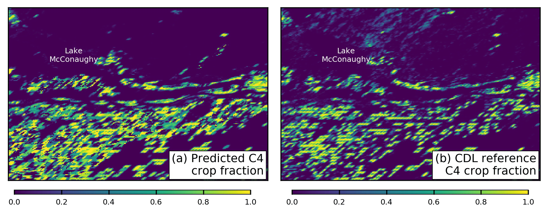
Figure 8 C4 crop fraction of (a) SLOPE predicted and (b) CDL reference data in a 50×75 km² area in Keith County, Nebraska (red marker in Fig. 7a), in 2000. Only CDL data during 2008–2019 are used in the modeling procedure, and therefore (b) is independent of (a). The maps are shown with the sinusoidal projection.

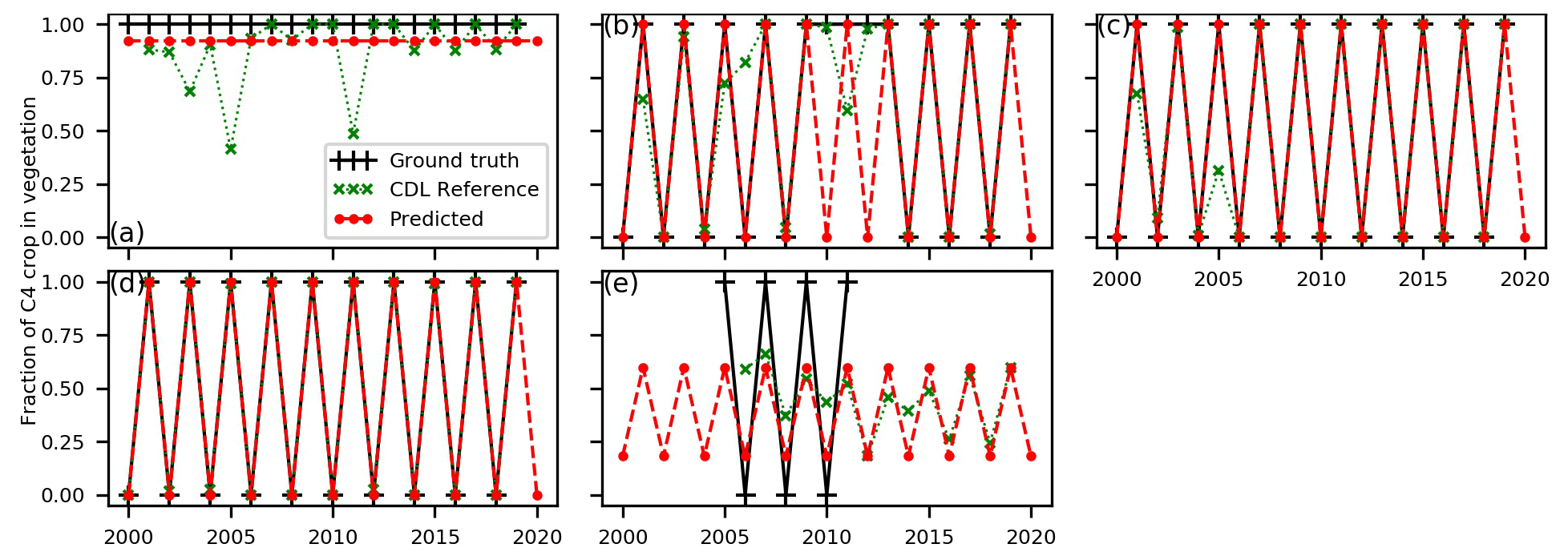
Figure 9 Comparison of fraction of C4 crop in vegetation between the field-collected ground truth, 250 m resolution CDL data and 250 m resolution SLOPE predictions at six AmeriFlux sites (Table S3) in the US Corn Belt from 2000 to 2020. (a) US-Ne1 (uncertainty: 0.17; Mead – irrigated continuous maize site). (b) US-Ne2 (uncertainty: 0.40; Mead – irrigated maize–soybean rotation site). (c) US-Ne3 (uncertainty: 0.18; Mead – rainfed maize–soybean rotation site). (d) US-Bo1 (uncertainty: 0; Bondville). (e) US-Ro1 (uncertainty: 0.16; Rosemount – G21). Uncertainty is the RMSE between the predicted and the CDL reference.

3.4 Performance of GPP

SLOPE SANIR_V shows a strong linear correlation with iPUE (Fig. 10). When data from all 49 sites (324 site years) are used together, the SANIR_V–iPUE relationship has an overall R² value of 0.73 (Fig. 10a). This is composed of an R² value of 0.92 from C4 species (Fig. 10b) and 0.70 from C3 species (Fig. 10c). C3 species can be further decomposed into six PFTs (Fig. 10d–i), among which cropland has the highest R² value up to 0.80 (Fig. 10i), whereas evergreen needleleaf forest has the lowest value of 0.46 (Fig. 10d). This relatively weak iPUE–SANIR_V relationship is expected because evergreen needleleaf forest tends to allocate resources for leaf construction and maintenance at large timescales and does not have much flexibility to change canopy structure and leaf color as a response to varying environment at small timescales (Badgley et al., 2019; Chabot and Hicks, 1982). Previous studies found that changes in the xanthophyll cycle instead of chlorophyll concentration or absorbed PAR explained the seasonal variation of photosynthetic capacity in evergreen needleleaf forest (Gamon et al., 2016; Magney et al., 2019). Therefore, SIF was suggested by some studies as a better proxy of photosynthetic capacity in this ecosystem (Smith et al., 2018; Turner et al., 2020), though satellite SIF has coarser spatial resolution, shorter temporal coverage, larger temporal latency and a lower signal-to-noise ratio than SANIR_V. In addition, the relatively weak iPUE–SANIR_V relationship is also partly because of the small value ranges in both SANIR_V and iPUE.

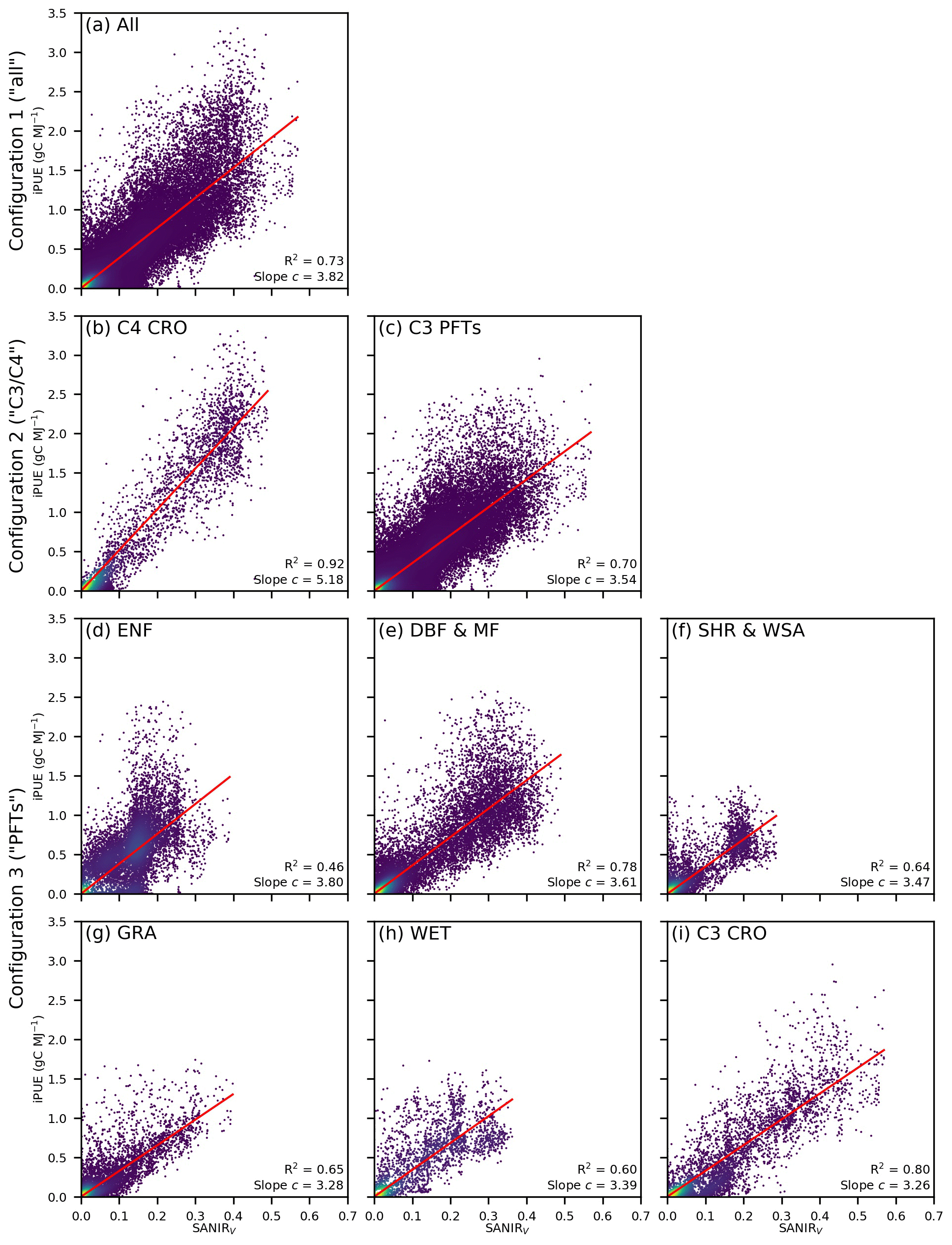
Figure 10 Comparison between SANIR_V and iPUE over different subsets. The slope value of the SANIR_V–iPUE relationship is the model parameter c (Eq. 5). Panel (a) is used by the model configuration 1 (all). Panels (b) and (c) are used by the model configuration 2 (C3–C4), which is actually used by SLOPE. Panels (b) and (d)–(i) are used by the model configuration 3 (PFTs).

The overall slope is 3.82 gC MJ⁻¹ for all data (Fig. 10a). A distinct difference is found between C4 (5.18; Fig. 10b) and C3 (3.54; Fig. 10c) species, suggesting the importance of separating C4 from C3 species in modeling. The slope values vary to a limited degree within C3 species (Fig. 10d–i), ranging from 3.26 gC MJ⁻¹ (cropland; Fig. 10i) to 3.80 gC MJ⁻¹ (evergreen needleleaf forest; Fig. 10d), indicating the insignificance of separating different PFTs. It is worth mentioning that the SANIR_V–iPUE relationship has a zero intercept because of the successful removal of the soil impact.

A 100-time-repeated 5-fold cross validation reveals the robustness of the SANIR_V–iPUE relationships (Fig. 11). Here the repeated cross validation means the whole GPP dataset from all 49 sites (324 site years) is randomly split into five folds, four folds for training and one fold for testing, and the process is repeated 100 times yielding 500 training–testing splits in total. In all subsets, the uncertainties of the iPUE coefficient c (the slope of the SANIR_V–iPUE relationship) are less than 1 % (Fig. 11a). When using the three different model configurations, the model performances in simulating the whole training–testing datasets also show little variation (Fig. 11b), in general <0.5 % and <1.5 % for the training and testing datasets, respectively. Moreover, the R² values between training and testing datasets, and between C3–C4 and PFT-based configurations are almost identical (∼ 0.76). These results suggest using c_C4=5.18 (Fig. 10b) and c_C3=3.54 (Fig. 10c) in SLOPE is reasonable. The 95 % confidential intervals of c for C4 and C3 species (Fig. 11a) are used as their uncertainties in SLOPE.

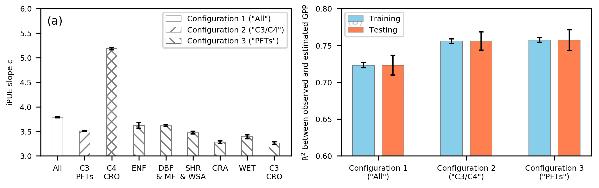
Figure 11 Statistics of the SANIR_V–iPUE relationship from cross validation. (a) Slopes of the SANIR_V–iPUE relationship over different subsets. (b) R² between AmeriFlux GPP and estimated GPP using different model configurations for the training and testing datasets, respectively. Error bars in both subplots indicate 95 % confidential intervals over 500 experiments.

SLOPE GPP demonstrates detailed and distinctive spatial variations in the CONUS (Fig. 12a). The Corn Belt is the most productive area, largely contributed by the C4 crop corn whose GPP could reach up to 30 gC m⁻² d⁻¹ (Fig. 13a). Forested areas in the eastern US show medium GPP values, followed by forests and croplands in the western US. Grasslands and shrublands in the central and western US generally show low productivity. On this example day, the R² of spatial patterns between GPP and SANIR_V, GPP and C4 fraction, and GPP and PAR across the CONUS are 0.89, 0.34 and 0.01, respectively. SANIR_V, an integrated vegetation index containing information of both FPAR and LUE (Eq. 4), explains the majority of GPP spatial variation. C4 fraction mainly contributes to the distribution and magnitude of the peak in GPP spatial variation. Although PAR does not influence the nationwide GPP spatial variation, it regulates GPP values at local scale. For example, northeastern Nebraska shows smaller GPP values than southeastern Nebraska in spite of a similar SANIR_V (Fig. 4a) and C4 fraction (Fig. 7a) because of smaller PAR values (Fig. 2a). At a small scale (e.g., within a county), the 250 m resolution (∼ 0.06 km² per pixel) SLOPE GPP is close to revealing field-level heterogeneity, considering that the mean and median crop field sizes in the CONUS are 0.19 and 0.28 km², respectively (Yan and Roy, 2016). For example, Fig. 13a shows large contrast in GPP, but Fig. 13b is more homogeneous. This is because corn reaches peak growing season in early July when soybean canopy is still open and sparse. SLOPE GPP with its pixel size much smaller than field area is therefore able to show GPP difference between corn and soybean. In late August, corn turns yellow, while soybean is still green and active, and therefore they have similar GPP values considering corn is C4, while soybean is C3. We suggest that the 250 m resolution makes a big difference compared to existing global GPP products whose spatial resolutions are at least 500 m (∼ 0.25 km² per pixel). Quantitative uncertainty is provided for each SLOPE GPP estimate (Eq. 8). The spatial pattern shows that the Corn Belt has the largest uncertainty (Fig. 12b; e.g., 5 gC m⁻² d⁻¹) due to the considerable contribution from the uncertainty of the C4 fraction (Fig. 7b).

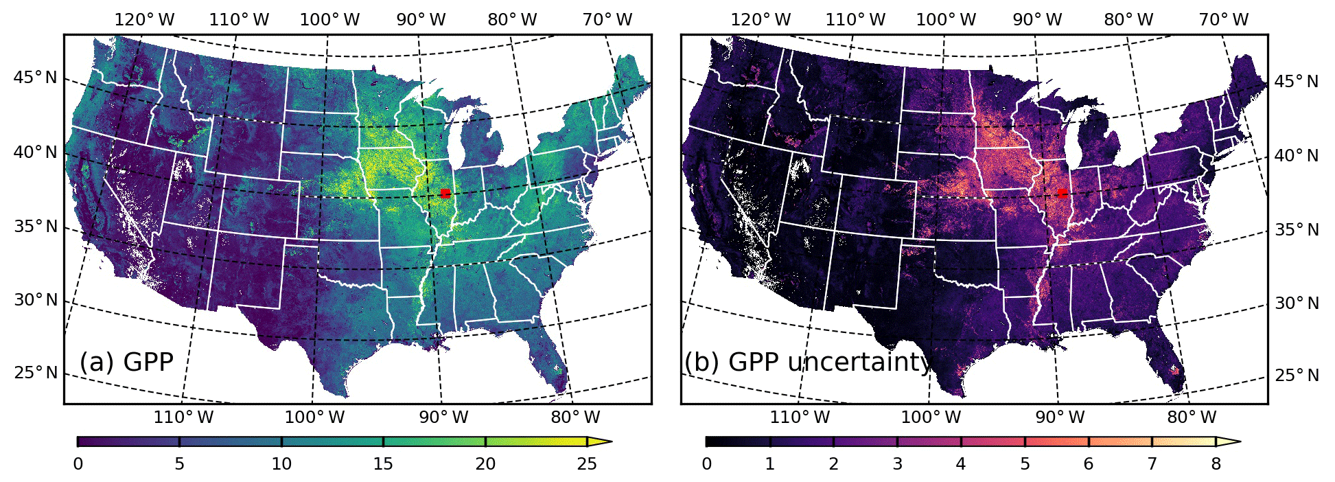
Figure 12 Spatial distribution of 250 m resolution (a) GPP (gC m⁻² d⁻¹) and (b) GPP uncertainty (gC m⁻² d⁻¹) across the CONUS on 10 July 2020.

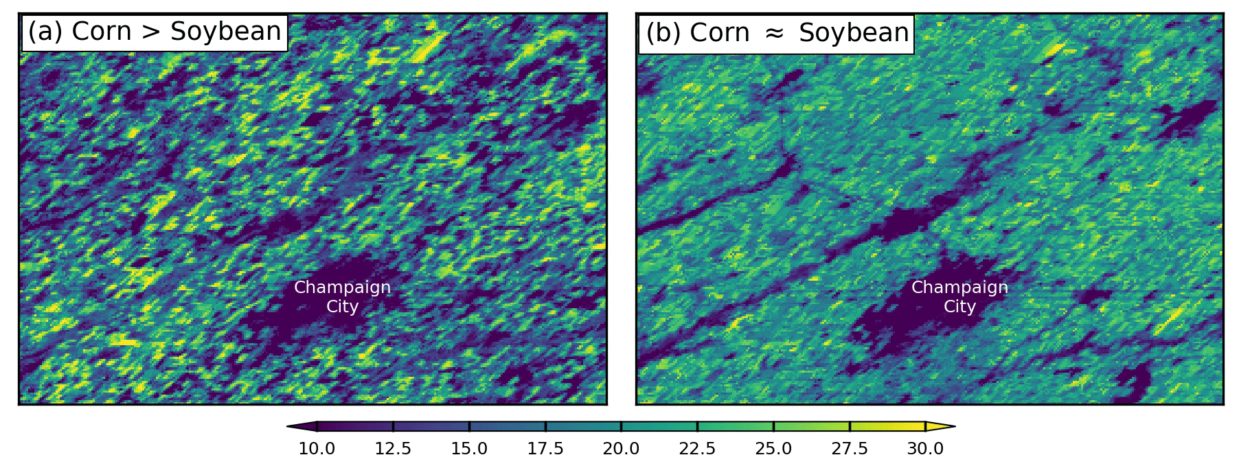
Figure 13 GPP (gC m⁻² d⁻¹) in a 50 × 75 km² area in Champaign County, Illinois (red marker in Fig. 12a), on (a) 10 July 2020 and (b) 20 August 2020. The maps are shown with the sinusoidal projection.

SLOPE GPP agrees fairly well with the ground truth from the AmeriFlux sites (Fig. 14). Across all of the 49 sites (328 site years; Fig. 14a), SLOPE GPP achieves an overall R² value of 0.85, RMSE of 1.63 gC m⁻² d⁻¹ and relative error of 37.8 %. For individual sites (Fig. 14b), the median R² and RMSE values are 0.80 and 1.69 gC m⁻² d⁻¹, respectively. C4 cropland generally shows the highest median R² value (0.94), followed by deciduous broadleaf forest and mixed forest (0.88) and C3 cropland (0.87). The lowest median R² value (0.69) is observed for evergreen needleleaf forest. With regard to RMSE, smaller median values are found in grassland (1.09 gC m⁻² d⁻¹), shrubland and woody savannah (1.48 gC m⁻² d⁻¹), and deciduous broadleaf forest and mixed forest (1.48 gC m⁻² d⁻¹), whereas C3 (2.15 gC m⁻² d⁻¹) and C4 (2.01 gC m⁻² d⁻¹) cropland tend to have larger RMSE values.

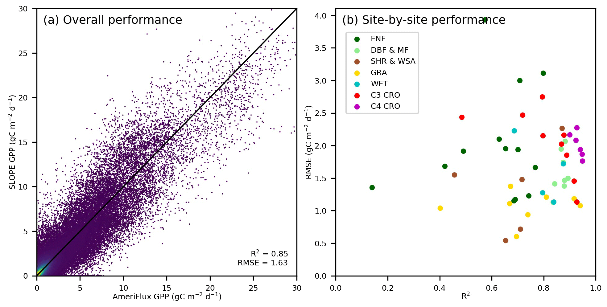
Figure 14 Performance of the SLOPE GPP. (a) Comparison between AmeriFlux GPP and SLOPE GPP across all sites. (b) R² and RMSE of individual sites. Sites with a C3–C4 rotation are separated into C3 CRO and C4 CRO.

SLOPE GPP generally captures seasonal and interannual variations of AmeriFlux GPP for different PFTs (Fig. 15). At the evergreen needleleaf forest site US-Blo (Fig. 15a), the GPP seasonal cycle is mainly driven by PAR, as the iPUE indicated by SANIR_V is fairly stable (Fig. 6a). At the deciduous broadleaf forest site US-Ha1 (Fig. 15b), the start of the season and the end of the season agree well between AmeriFlux GPP and SLOPE GPP. At the open-shrubland site US-Whs (Fig. 15c), the quick rise and drop of GPP in response to the start and end of the wet season are clearly observed in SLOPE GPP. Even the double-peak pattern in 2011 can be observed in SLOPE GPP. At the grassland site US-AR1 (Fig. 15d), the impact of a severe drought in the southern Great Plains in 2011 is distinct in SLOPE GPP, as the GPP values in 2011 are only about half of those in 2010 and 2012. At the cropland site US-Bo1 (Fig. 15f), the rotation-caused year-to-year variation is distinct, indicated by higher values in odd-numbered years with C4 crop corn planted and lower values in even-numbered years with C3 crop soybean planted (Fig. 9d). The lowest GPP peak is observed in 2012 when a severe drought attacked the central US.

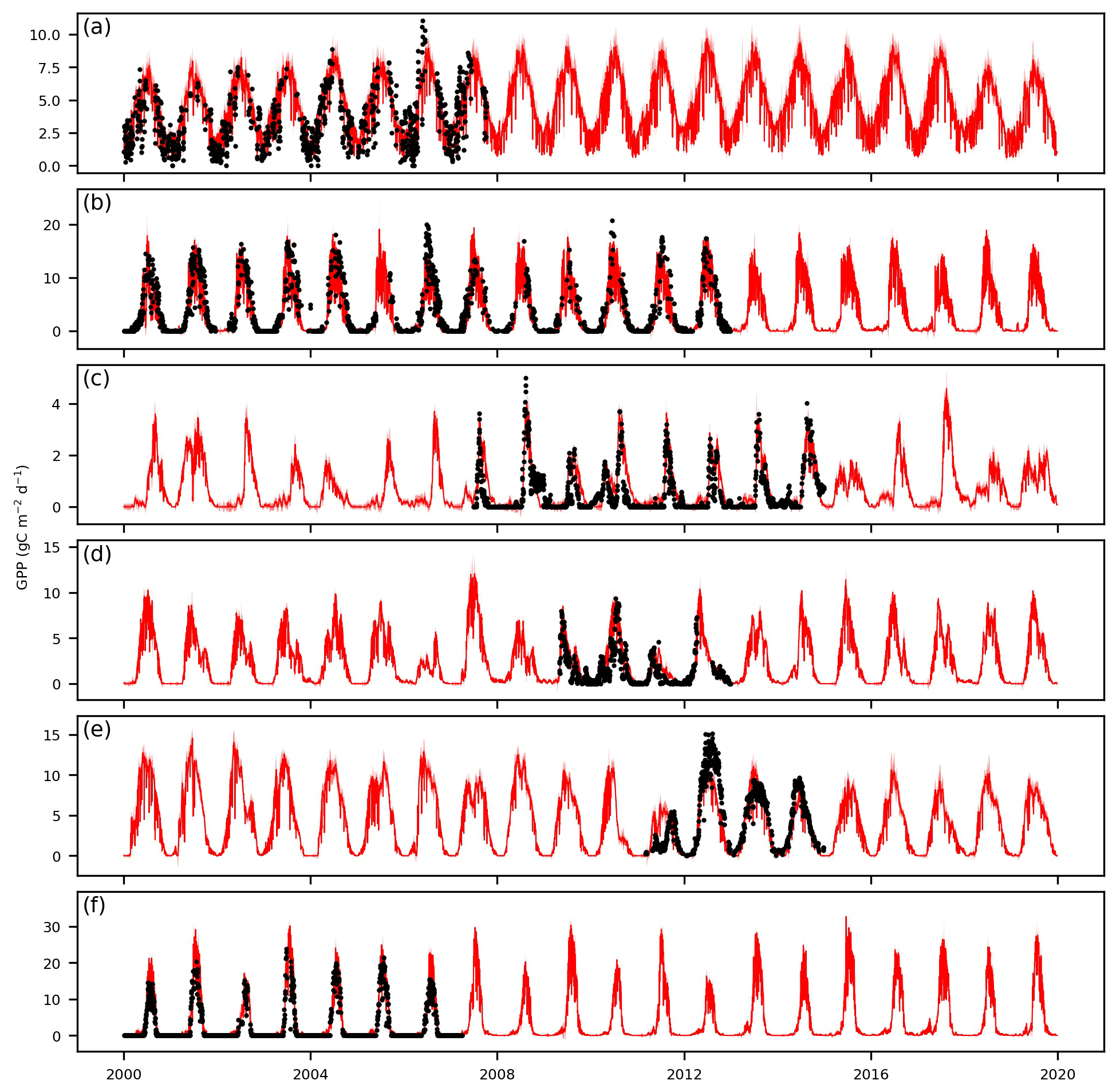
Figure 15 Comparison between AmeriFlux (black dots) and SLOPE (red curves) daily GPP at six AmeriFlux sites (Table S3) from 2000 to 2019. (a) US-Blo (evergreen needleleaf forest, ENF). (b) US-Ha1 (deciduous broadleaf forest, DBF). (c) US-Whs (open shrubland, OSH). (d) US-AR1 (grassland, GRA). (e) US-Myb (wetland, WET). (f) US-Bo1 (cropland, CRO). Shaded areas indicate uncertainties of SLOPE GPP.

4 Data availability and data format

The archived daily 250 m resolution SLOPE GPP data product from 2000 to 2019 is distributed under a Creative Commons Attribution 4.0 License. It is publicly available at NASA's Oak Ridge National Laboratory Distributed Active Archive Center (ORNL DAAC) with a DOI of https://doi.org/10.3334/ORNLDAAC/1786 (download page: https://daac.ornl.gov/daacdata/cms/SLOPE_GPP_CONUS/data/, last access: 20 January 2021) (Jiang and Guan, 2020). Data from 2020 are available from the authors upon request. All data are projected in the standard MODIS Land Integerized Sinusoidal tile map projection and are stored in GeoTIFF format files with a data type of signed 16 bit integer. Each processing tile has a size of 4800 pixels by 4800 pixels, representing a land region of approximately 1200 km by 1200 km . In addition to the GPP product, SLOPE PAR, SANIR_V and C4 fraction, along with their uncertainties, are also released. These datasets are also stored in the same spatial projection and file format with the GPP dataset. PAR (resampled from 1 km to 250 m to be consistent with GPP) and SANIR_V are provided on a daily basis, whereas C4 fraction is provided on an annual basis. A README file is provided along with the SLOPE product, which instructs the usage of the data.

5 Conclusions

This study produces a long-term and real-time (2000–present) GPP product with daily and 250 m spatial and temporal resolutions. The product is based on a remote-sensing-only (SLOPE) model, which uses accurate PAR, soil-adjusted NIR_V and dynamic C4 fractions as inputs. Evaluation against AmeriFlux ground-truth GPP shows that the SLOPE GPP product has a reasonable accuracy, with an overall R² of 0.85 and RMSE of 1.63 gC m⁻² d⁻¹. To demonstrate the real-time capacity of the SLOPE GPP product, the latest GPP data on 2 November 2020, 2 d prior to the revision of this paper, is shown in Fig. S7. The spatiotemporal resolution and instantaneity of the SLOPE GPP product are higher than existing global GPP products, such as MOD17, VPM, GLASS, FLUXCOM and BESS. We expect this novel GPP product can significantly contribute to various researchers and stakeholders in fields related to the regional carbon cycle, land surface processes, ecosystem monitoring and management, and agriculture. The approaches used in this study, in particular, the derivation of SANIR_V, can also be applied to any other satellite platform with the two most classical bands: red and NIR, for example, SaTellite dAta IntegRation (STAIR) from Landsat–MODIS fusion data, which has daily, 30 m spatiotemporal resolution and can be applied at a large scale (Jiang et al., 2020; Luo et al., 2018); commercial Planet Labs data with a daily interval and spatial resolution up to 3m (Houborg and McCabe, 2016; Kimm et al., 2020); and the Advanced Very High Resolution Radiometer (AVHRR) with a temporal coverage as far back as 1982 (Franch et al., 2017; Jiang et al., 2017). However, caution should be used in the interpretation of GPP seasonal trajectory in evergreen needleleaf forests because of the relatively poor relationship between SANIR_V–iPUE and GPP magnitude in southwestern US grasslands because of the ignorance of the fraction of C4 grasslands. Finally, although the SLOPE product has been generated from 2000 to present, caution should also be used in the interpretation of the long-term trend because the SLOPE model, as many other LUE models, does not explicitly consider the CO₂ fertilization effects on vegetation productivity.