the Creative Commons Attribution 4.0 License.
the Creative Commons Attribution 4.0 License.
 | 18 May 2021
A new global gridded sea surface temperature data product based on multisource data
Mengmeng Cao
Yibo Yan
Jiancheng Shi
Han Wang
Tongren Xu
Zijin Yuan
Sea surface temperature (SST) is an important geophysical parameter that is essential for studying global climate change. Although sea surface temperature can currently be obtained through a variety of sensors (MODIS, AVHRR, AMSR-E, AMSR2, WindSat, in situ sensors), the temperature values obtained by different sensors come from different ocean depths and different observation times, so different temperature products lack consistency. In addition, different thermal infrared temperature products have many invalid values due to the influence of clouds, and passive microwave temperature products have very low resolutions. These factors greatly limit the applications of ocean temperature products in practice. To overcome these shortcomings, this paper first took MODIS SST products as a reference benchmark and constructed a temperature depth and observation time correction model to correct the influences of the different sampling depths and observation times obtained by different sensors. Then, we built a reconstructed spatial model to overcome the effects of clouds, rainfall, and land interference that makes full use of the complementarities and advantages of SST data from different sensors. We applied these two models to generate a unique global 0.041∘ gridded monthly SST product covering the years 2002–2019. In this dataset, approximately 25 % of the invalid pixels in the original MODIS monthly images were effectively removed, and the accuracies of these reconstructed pixels were improved by more than 0.65 ∘C compared to the accuracies of the original pixels. The accuracy assessments indicate that the reconstructed dataset exhibits significant improvements and can be used for mesoscale ocean phenomenon analyses. The product will be of great use in research related to global change, disaster prevention, and mitigation and is available at https://doi.org/10.5281/zenodo.4419804 (Cao et al., 2021a).
- Article
(10776 KB) - Full-text XML
- BibTeX
- EndNote


The temperature at the interface between the atmosphere and ocean, known as the sea surface temperature (SST), is an important indicator of Earth's ecosystem (Hosoda and Sakaida, 2016). SSTs are widely used in atmospheric and oceanographic studies, such as in atmospheric simulations, climate change monitoring, and studies of marine dynamic environments (Kawai and Wada, 2007; Martin et al., 2007; Peres et al., 2017; Reynolds and Smith, 1995). In addition, the oceans cover 70 % of Earth's surface. A small variation in the ocean temperature exerts strong impacts on regional and even global climate change, energy exchange, and the environment due to the unique physical characteristics of the oceans, including their high heat capacity (Yan et al., 2020; Varela et al., 2018). The rise of ocean temperatures will release huge amounts of heat, affect atmospheric movement, and produce many chain reactions, causing reductions in the CO2 content of seawater, the occurrence of extreme weather, the melting of sea ice in the polar region, and the rise of sea level, all of which will impact the survival of marine life, marine production, and human life (Sakalli and Basusta, 2018). Thus, it is essential to accurately monitor changes in SST.
It is difficult for traditional SST measurements based on buoys, platforms, and voluntary ships to obtain large-scale and synchronous SST data due to the large gaps present in the data over both space and time. Compared to the traditional in situ SST monitoring approach, remote sensing technology has advantages in terms of large-scale and dynamic monitoring and has been used to acquire global ocean SST observation data (Li and He, 2014). Satellite SST data include thermal infrared and microwave radiometer SST data. Retrievals from satellite thermal infrared sensors can provide global SSTs at high temporal frequencies and spatial resolutions of typically 1–4 km with low uncertainty (Alerskans et al., 2020). For example, series sensors such as the Moderate Resolution Imaging Spectroradiometer (MODIS) and Advanced Very High Resolution Radiometer (AVHRR) can measure global SSTs with high resolutions and high accuracies. These observations are unfortunately greatly influenced by the atmospheric environment. In cases of aerosol contamination and cloud cover, it is impossible to obtain effective observations, resulting in spatial discontinuities and low quality in the collected data (Guan and Kawamura, 2003; Hosoda et al., 2015; Y. Liu et al., 2017). In contrast to thermal infrared measurements, microwave sensors are less affected by clouds and aerosol concentrations (Alerskans et al., 2020; Mao et al., 2019). Therefore, microwave sensors can observe SST information at all times and in all weather conditions except rain, and they also have high temporal resolutions and can quickly cover the whole surface of Earth (Wentz et al., 2000). As a result, microwave sensors play important roles in monitoring the temporal and spatial changes in SSTs on global and continental scales and have also been developed into mature remote sensing products, such as the TRMM Microwave Imager (TMI), the WindSat onboard Coriolis, and the Advanced Microwave Scanning Radiometer for Earth Observation System (AMSR-E), which have been widely used to retrieve SSTs (Gentemann, 2014; Ng et al., 2009; Purdy et al., 2006). However, the spatial resolutions of passive microwave sensors are very coarse and are greatly affected by land and sea surface wind and waves, which makes it impossible to obtain detailed information about SSTs (Gentemann et al., 2010; M. Liu et al., 2017). In addition, due to the influence of imaging orbit gaps, microwave-based products produce spatial gaps. Therefore, the SST information obtained by a single satellite remote sensor is often incomplete and limited and cannot fully meet the user's demand for a dataset with a high resolution, high precision, and full spatiotemporal coverage. Fortunately, the simultaneous availability of multiple satellite sensors provides highly complementary information, enabling the production of high-quality unified SST datasets with improved global coverage (Guan and Kawamura, 2004; Shi et al., 2015; Thiebaux et al., 2003).
Many SST fusion algorithms use multiple satellites and in situ data to take advantage of the strengths of each SST observation and solve the above issues; these algorithms include objective analysis (OA), optimal interpolation (OI), three-dimensional variational (3D-Var), and Kalman filtering (KF) (Chao et al., 2009b; Li et al., 2013; Smith and Reynolds, 2003). Bretherton et al. (1976) first applied OA in a study of ocean data. OI was developed on the basis of OA, and in OI, background information is introduced in the analysis process. Although there is no physical constraint, the OI has a perfect mathematical form, which statistically takes into account the influence of the relative position changes of different observation points on the error covariance. The OI algorithm is simple and easy to use and has become one of the main methods currently used for SST fusion. For example, Reynolds and Smith (1994) used the OI method to fuse in situ data from ships, buoys, and satellites to produce OISST products that are widely used. The other SST analysis data product, RTG-SST from the National Centers for Environment Prediction (NCEP), is also obtained by the OI method. In addition, based on the Modular Ocean Model (MOM), the National Science Foundation and the National Oceanic and Atmospheric Administration established the Simple Ocean Data Assimilation system (SODA) by the OI method (Carton et al., 2018; Carton and Giese, 2008). Based on the Modular Ocean Model version 4p1 (MOM4), the Australian Bureau of Meteorology established marine forecasting systems covering Australia, nearby regions, and the globe through the ensemble optimal interpolation (EnOI) method (Oke et al., 2008). However, in practice, to reduce the computational burden, the OI algorithm is usually only applied using data near the analysis point, and there is often a certain degree of subjectivity. Methods such as Var and KF have been proposed to overcome these problems, and these methods have been widely used. For example, Zhu et al. (2006) developed a new 3D-Var-based Ocean Variational Analysis System (OVALS), which can effectively improve estimations of temperature and salinity by assimilating various observed data. Li et al. (2008) applied a new 3D-Var data assimilation scheme to a retroactive real-time forecast experiment, and favorable results were obtained. In terms of operational applications, some institutions in Canada, the United Kingdom, the United States, and China have used this method to establish ocean environmental forecast and analysis systems based on different oceanic general circulation models (Burnett et al., 2014; Chassignet et al., 2009; Han et al., 2011; Storkey et al., 2010). Huang et al. (2008) filled in the missing parts of satellite SST data with the kriging interpolation method based on the slowly changing characteristics of SSTs and then used KF to coordinate the variation error and interpolation error of the obtained SSTs. Finally, the interpolation and filtered SST data were fitted to realize SST filling. Wang et al. (2010) used the KF method to fuse the AVHRR SST and AMSR-E SST products to produce daily, spatially continuous SST data with a spatial resolution of approximately 2 km. However, a daily variation correction was not carried out before the fusion, and the model processing error was not taken into account, which brought great uncertainty to the fusion results.
Although many studies have tried to improve the accuracy and spatial coverage integrity of SST products, especially the sea temperature fusion products in deep ocean areas with high accuracy (Dash et al., 2011), some ocean surface (skin) temperature products still contain some deficiencies. Different methods can be used to obtain ocean surface temperature, but they actually represent temperature information at different ocean depths, and the observation time is also inconsistent (Castro et al., 2004; Wick et al., 2004). The sea temperature observed by traditional sites is deeper than the temperature observed by remote sensing. Even if they are all the temperatures retrieved from remote sensing, the temperatures retrieved from thermal infrared and microwaves are from different ocean depths. The sea temperature observed by thermal infrared is the skin temperature, and the sea temperature observed by microwaves is a bit deeper than the depth observed by thermal infrared. The sea surface temperature obtained by the assimilation model should also be different. In addition, some products have problems with missing pixels and relatively low accuracies near coasts and the edges of sea ice due to the characteristics of the remote sensing products themselves and the insufficiencies of fusion methods (Xie et al., 2008). Some assimilation products (e.g., ERA5, ECMWF Re-Analysis) of multisource oceanic data can solve state estimations of large-scale oceanic ocean phenomena well (Hersbach et al., 2020), but these products cannot meet the needs of near-shore or small- and medium-scale phenomena.
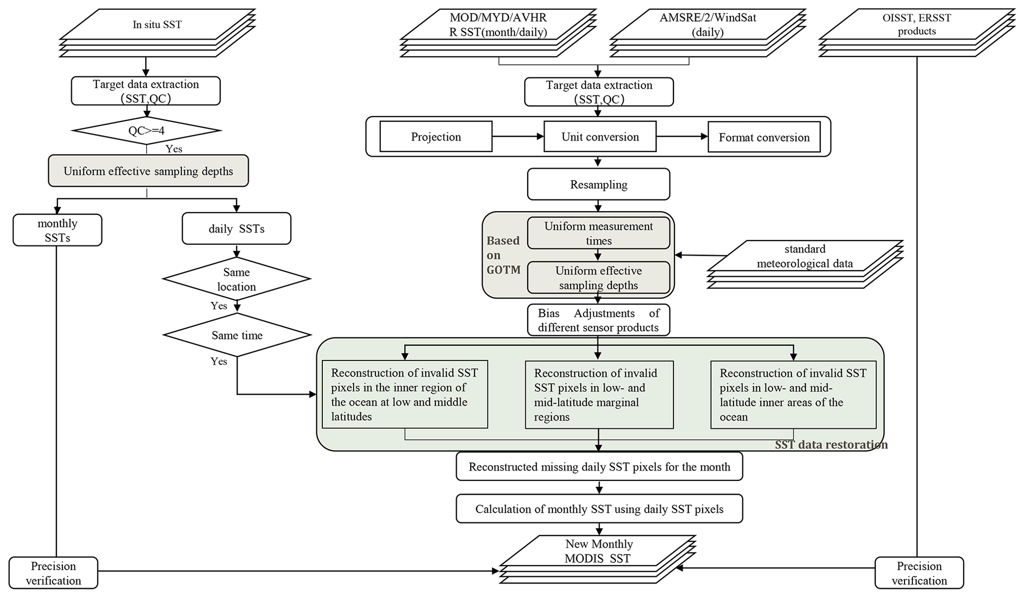
In order to obtain a long-term series of major global meteorological disaster remote sensing datasets with high spatiotemporal consistency based on the current global multi-source remote sensing data and ground observation site data, we constructed a temperature depth and observation time correction model to eliminate the sampling depth and temporal differences among different data, and we built a reconstructed spatial model that filters out missing pixels and low-quality pixels from the monthly MODIS SST dataset and reconstructs them based on daily in situ SST data and daily satellite SST retrieval data from two infrared (MODIS and AVHRR) and three passive microwave (AMSR-E, AMSR2, WindSat) radiometers to generate a high-quality unified global SST product with long-term (2002–2019) spatiotemporal continuity. The validation and cross comparisons with in situ observations and other SST products were made to prove that the new reconstructed SST dataset is reliable and is suitable for regional or global SST studies.
2.1 Satellite data retrievals
Thermal infrared and microwave radiometers on sun-synchronous satellites are the primary technical tools used to obtain global SST, and collectively these sensors provide highly complementary information with which a new SST product can be generated. The AVHRR and MODIS sensors, which cover the global ocean, were selected as sources of thermal infrared radiometer data. To reduce the data gaps present in thermal infrared data resulting from cloud and water vapor contamination, the inclusion of microwave radiometer data from polar-orbiting satellites is essential; in this study, AMSR-E, WindSat, and AMSR2 are the main sources of microwave data.
The MODIS sensor is on board the Terra and Aqua spacecraft: the sensor has an ascending local equatorial crossing time of 13:30 in the case of the Aqua spacecraft and a 10:30 descending equatorial crossing time for the Terra spacecraft. The daily and monthly L3m global SST products (Day and Night) of the MODIS sensor from Terra and Aqua are available starting from February 2000 and July 2002, respectively, with a 0.041∘ spatial resolution; these datasets were mainly used to reconstruct high-quality SST data and are available through the website https://oceandata.sci.gsfc.nasa.gov/ (last access: 14 January 2020). The standard deviation obtained in a data comparison was better than 0.43 ∘C, as determined by comparison of the SST data with coincident ferry observations (Barton and Pearce, 2006). Each pixel of these SST data is associated with a numerical quality level stored in SST_flags whose value ranges, in order of descending quality, from 0 to 4. Clear data of the best quality are limited to the satellite zenith angles, <55∘. Clear pixels at satellite angles >55∘ have good quality, with quality levels of 1. Pixels with a quality level >1 may have very large differences between the retrieved SST and the reference SST due to significant cloud contamination or various other problems (https://oceancolor.gsfc.nasa.gov/atbd/sst/, last access: 14 January 2020). Therefore, these pixels are not used for scientific research.
The AVHRR sensor is on board NOAA polar-orbiting satellites, has six bands ranging in wavelength from visible to infrared (one visible, two near-infrared, and three thermal infrared) and can cover the globe twice a day. The twice-daily (day and night) AVHRR 4 km SST data product is produced by the NOAA National Centers for Environmental Information and is available through the website https://data.nodc.noaa.gov/pathfinder/Version5.3/L3C/ (last access: 6 February 2020). The standard deviation obtained in a data comparison is approximately 0.68 ∘C, as determined by a comparison of the AVHRR products with coincident ferry observations (Barton and Pearce, 2006). The data also provided a quality index for each pixel based on the evaluation test results stored in the pathfinder_quality_level metric, which allows the identification of cloudy pixels and/or suspicious observations, with the quality level 0 representing the worst quality and the quality level 7 being the best (Pisano et al., 2016). In our data processing method, we only considered values with quality flags 4–7.
The AMSR-E sensor is on board the Aqua satellite and is a dual-polarization microwave scanning radiometer with six frequency channels in the range of 6–89 GHz. The AMSR-E instrument was in orbit for nearly 10 years but was discontinued in October 2011, owing to an antenna rotation problem. The AMSR2 sensor, on board the Global Change Observation Mission-Water 1 (GCOM-W1) satellite, was launched in May 2012 to continue the Aqua/AMSR-E observations and ensure the continuity of SST data (Zabolotskikh et al., 2015). AMSR2 has the same channels as did AMSR-E, with a 7.3 GHz channel added to help alleviate radio frequency interference. However, SST information collected from the AMSR2 sensor was not provided until mid-2012. To ensure that there is an uninterrupted consistent long-term microwave SST time series that can be used to reconstruct a high-quality SST product, a WindSat polarimetric radiometer was used to bridge the gap between the AMSR-E and AMSR2 products. The daily L3 SST products (ascending and descending passes) of AMSR-E and AMSR2, available from June 2002 and July 2012, respectively, with 0.1∘-grid spatial resolutions, were used to reconstruct high-quality SST data and are available through the website https://gportal.jaxa.jp/gpr/search/ (last access: 9 February 2020). The accuracies of AMSR-E and AMSR2 are approximately 0.75 and 0.56 ∘C, respectively, as determined by comparisons with buoy data (Sun et al., 2018). Daily WindSat SST datasets on a global 25 km grid (ascending and descending passes) were downloaded online (http://www.remss.com/missions/windsat, last access: 16 February 2020), and their accuracies are very close to that of AMSR-E, as determined by comparisons with buoy data (Banzon and Reynolds, 2013; Gentemann, 2011).
2.2 In situ observations
In situ observations of SST from 2002–2019 were used for the reconstruction of the new SST product and the validation of both the satellite-obtained SST data and the new product. The SST data observed in situ used in this study consist of SSTs from the Version 2.1 NOAA in situ Quality Monitor (iQuam), which includes updated observations every 12 h with a 2 h latency. The SST data from iQuam include observations from drifters, ships, tropical (T-) and coastal (C-) moorings, Argo floats, high-resolution (HR) drifters, IMOS ships, and coral reef water (CRW) buoys, and the data can be obtained from ftp://ftp.star.nesdis.noaa.gov/pub/sod/sst/iquam/v2.10/ (last access: 21 January 2020). Quality control of the data, including basic screening, duplicate removal, plausibility, platform tracks, referencing, and cross-platform and SST spike checks, was performed by the NOAA Center for Satellite Application and Research (Xu and Ignatov, 2014). Only SSTs assigned the best quality flag (i.e., level 5) were used in this study. To ensure the independence of the data reconstruction and the accuracy verification process, the data obtained from all spatially coincident in situ observations of SST were randomly divided into two completely independent subsets by the jackknife method (Benali et al., 2012). Subset 1 accounts for 80 % of the total number of in situ observations, which were used to reconstruct the MODIS SST data. Subset 2 accounts for 20 % of the total number of in situ observations, which were used to verify the accuracy of the reconstruction results. The spatially coincident criterion restricts the maximum distance between in situ measurements and the center of the satellite image grid cells to within 2.3 km, which is approximately half the spatial resolution of MODIS, so that the in situ observations always fall within the MODIS SST pixels (Minnett, 1991; Pisano et al., 2016).
2.3 Ancillary data
ERA-Interim, a climate reanalysis product produced by the European Centre for Medium-Range Weather Forecasts (ECMWF), was discontinued on 31 August 2019 and has been superseded by the ERA5 reanalysis product produced by the ECMWF. The ERA5 dataset is the latest climate reanalysis product, providing hourly data on atmospheric, land, and oceanic climate parameters together with estimates of uncertainty. The 10 m wind component U, 10 m wind component V, 2 m temperature, 2 m dew point temperature, sea surface temperature, relative humidity, cloud cover, and other data from the two datasets with 0.25∘ spatial resolutions were used to calculate the heat, momentum, and fluxes between the ocean and the atmosphere as well as the incoming solar radiation. These data can be obtained from https://apps.ecmwf.int/datasets/ (last access: 15 January 2020).
Since MODIS SST data have a high accuracy and spatiotemporal resolution which can be used to capture mesoscale phenomena in the oceans, a combination of MODIS SSTs from Aqua and Terra is a good way to improve the spatial coverage of SST data. However, SSTs are retrieved using the thermal infrared bands which are influenced much by clouds, so SST data cannot be provided when they have clouds in the sky, and SST retrievals are also influenced by atmospheric aerosols. Some other factors related to radiometers can also contaminate SST observations, such as the viewing geometry, spectral response, and noise level of each sensor (Kilpatrick et al., 2015). Due to these effects, MODIS SST data often have problems involving low-quality or missing pixels. Statistical analysis performed during the study period indicated that the missing pixels present in the monthly SST records of Terra and Aqua during both daytime and nighttime generally cover 23.46 % and 28.06 % of the global ocean, respectively. In order to overcome these defects, we built a reconstructed spatial model that combines in situ station-based data and daily SST data from AVHRR, AMSR-E, AMSR2, and WindSat to generate a high-quality MODIS SST monthly dataset. Although the temperatures retrieved by different sensors are all ocean surface temperatures, they actually represent temperature information at different ocean depths which are caused by different frequencies of different sensor settings and inconsistent algorithms. The sea temperature observed by thermal infrared is the skin temperature, and the sea temperature observed by microwaves is a bit deeper than the depth observed by thermal infrared. In addition, the observation time of different observation methods may be inconsistent. Therefore, we proposed a temperature depth and observation time correction model to address the influence of time phase and sampling depth of different sensors. More details are given in the following sections. The overall methodology is illustrated in Fig. 1. This processing effectively retains the high-precision pixels in the original MODIS daily and monthly data, combines the calibrated ocean multi-source data with spatiotemporal information to reconstruct the low-quality and missing daily pixels, and finally replaces the low-quality and missing pixels in the monthly data.
3.1 Bias adjustment by constructing temperature depth and observation time correction model
3.1.1 Bias adjustment scheme for multisource remote sensing data
To combine oceanic multisource remote sensing data into the MODIS SST product, it is necessary to assume that the measured values represent the same quantities or to use some method to eliminate the differences among products. The ocean temperature data obtained by different sensors are different from those obtained by MODIS, and there are complex spatiotemporal differences. Figures 2 and 3 represent the difference distributions of the original MODIS and multisource daily SSTs in the daytime. Obviously, these multisource data cannot be directly used to reconstruct the valid pixels of MODIS SST data before the differences are corrected.
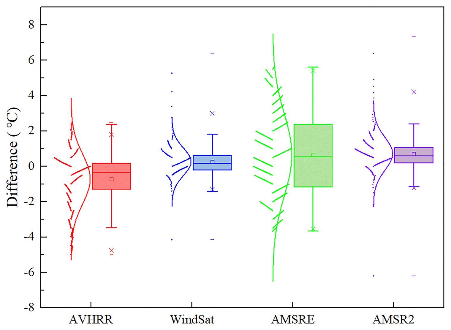
Figure 2Box chart with scatters of the differences in the original MODIS and multisource daily SSTs (AVHRR, WindSat, AMSR-E, AMSR2). The boxes are determined by the 25th and 75th percentiles. The whiskers are determined by the 5th and 95th percentiles. The data are plotted as scatters on the left of each box. A curve corresponding to a normal distribution is also displayed on top of each scatter plot.
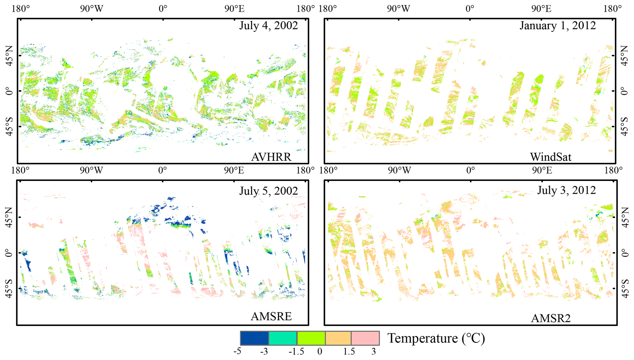
Figure 3Difference maps of the original MODIS and multisource daily SST products. Areas of missing data are blank.
The main source of the difference is the inconsistent wavelength or frequency range used by different sensors, which leads to the temperature information measured by the sensors from different ocean depths. The thermal infrared remote sensor measures the sea surface skin temperature at a depth of 10–20 µm, while the microwave remote sensor can retrieve the sea subcutaneous temperature at a depth of 1–1.5 mm (Minnett, 2003; Minnett et al., 2011). Therefore, the SSTs retrieved from various microwave radiometers (AMSR-E, WindSat, and AMSR2) are different from the SSTs measured by the MODIS radiometer. In addition, due to the difference of the inversion algorithm parameters, the sea temperature retrieved from the same type of sensor may also be different. For example, although the AVHRR sensor is an infrared remote sensor and its brightness temperatures represent the sea surface skin temperature, AVHRR SSTs correspond to subsurface SSTs because they are statistically regressed to coincident in situ buoy SSTs (Chao et al., 2009a; Kilpatrick et al., 2001; Pisano et al., 2016). Starting with the AVHRR Pathfinder Version 5.3, an average skin–subsurface temperature difference of 0.17 K, determined from Marine Atmospheric Emitted Radiance Interferometer (M-AERI) matchups, was used to eliminate the subsurface bias so that the SSTs were more closely tuned to the sea surface skin temperatures (Sea Surface Temperature-Pathfinder C-ATBD). MODIS SSTs are skin SSTs. MODIS retrievals are based on empirical coefficients derived by regressing MODIS brightness temperatures against in situ observations from drifting and moored buoys, but the regressed SSTs are converted to skin SSTs based on at-sea measurements. Thus, the SSTs retrieved from the AVHRR radiometer are different from the SSTs measured by the MODIS radiometer. In addition, MODIS and several other sensors used in this paper have different observation times and can obtain measurements at several different times throughout the diurnal cycle. The relationships among these observations are, however, not constant because there are significant diurnal variations in sea surface temperature resulting from constant changes in the atmosphere, solar heating, wind speeds, etc. (Kilpatrick et al., 2015; Luo et al., 2019; Minnett et al., 2019; Wick et al., 2004). This also results in differences between MODIS observations and those of other sensors. Therefore, compensating for measurement depths and times is conducive to reducing the uncertainty present in the reconstruction results before the multisource remote sensing data are combined into the MODIS SST product.
-
Compensating to ensure uniform effective sampling depths.
To solve the differences among MODIS and multisource daily SST products caused by the sampling depths, it is necessary to consider the differences as results of the cool skin effect and diurnal heating (Luo et al., 2020). The General Ocean Turbulence Model (GOTM) can model the SST signal at different depths by simulating the hydrodynamic and thermodynamic processes of vertical mixing in one-dimensional water columns in natural waters which has been successfully used to model the near-surface variability of ocean temperature (Karagali et al., 2017; Pimentel et al., 2018). General ocean models typically simulate the surface layer of 5–10 m as a uniform layer, and simulating such thin sea surface skin layers and subskin layers takes a long time. The GOTM can use a non-uniform grid and specifically encrypt the surface layer to quickly simulate the temperature of the sea surface skin layer and the subskin layer. For example, the top 50 m of the water column is resolved by using 50 vertical layers, which have higher resolution near the surface and gradually decrease with depth. The thickness of the first layer at the top of the water column is about 20 µm, and the thickness of each layer can be calculated according to Eq. (1).
where hk represents the thickness of layer K. D represents the depth. M is the number of layers, and dl and du show the zooming factors of the surface and bottom, respectively.
From this formula, the following grids are constructed:
-
results in equidistant discretization.
-
dl>0, du=0 results in zooming near the bottom.
-
dl=0, du>0 results in zooming near the surface.
-
dl>0, du>0 results in double zooming near both the surface and the bottom.
Furthermore, considering the cool skin effect that usually occurs in a molecular sublayer of the air–sea interface, a physical model for the skin (as shown in Eqs. 2 and 3) widely used to estimate the cold skin effect was integrated into the air–sea interaction module of the GOTM (Fairall et al., 1996; Saunders, 1967). The heat and momentum flux changes of each layer in the water column were integrated to more accurately simulate the skin effects of the SSTs.
where ΔT is the temperature variation (positive, representing that the surface is cooler than the bulk). Q is the net heat flux. K is the thermal conductivity of water. δ is the thickness of the change in temperature. λ is the empirical coefficient. V is the kinematic viscosity, and μ∗w is the friction velocity in the water. It is difficult to obtain λ in Eq. (2). Based on the observed data of the Tropical Ocean-Global Atmosphere Coupled Ocean–Atmosphere Response Experiment (COARE) program, Fairall et al. (1996) determined λ to be dependent on wind speed.
In this section, the conversion of SSTs between different depths can be conducted using the model by entering the SST measurement depth and the corresponding meteorological parameter values present during the measurement, including the wind speed at a 10 m height, the air temperature at a 2 m height above the sea surface, air humidity data, and cloud cover data from the ECMWF. Figure 4a and b show the variations in ocean temperatures at different depths and the differences between the sea surface skin temperatures and sea surface subskin temperatures simulated by the GOTM every half hour for a pixel with a longitude of 32.65∘ N and a latitude of 43.25∘ E from 1 July 2002 to 31 July 2002. When the wind speed is low, the infrared-measured SST is 0.1–0.2∘ lower than that obtained by microwave remote sensing. When the wind speed is high, the SSTs measured by the two sensor types are basically the same. By deducting this difference, the SSTs obtained by microwave remote sensing can be normalized to the SSTs obtained by infrared remote sensing.
-
-
Compensating to ensure uniform measurement times.
To solve the differences among the MODIS and multisource daily SST products caused by the varying measurement times, it is necessary to consider the diurnal variations in SST. The GOTM is based on the hydrodynamic and thermodynamic processes of water and comprehensively considers the effects of solar shortwave radiation, longwave radiation, latent heat, sensible heat, and cloudiness on diurnal variations in SST. The diurnal variations caused by differences in the absorption and attenuation of solar radiation of different water types are also considered. Therefore, the GOTM can accurately simulate diurnal variations in SST. The input data also come from the ECMWF reanalysis product and include the wind speed at a 10 m height, the air temperature at a 2 m height above the sea surface, air humidity data, and cloud cover data. Cloudiness is used to calculate oceanic radiant heating. Wind speed, air temperature, and relative humidity are used as inputs in the turbulence model to estimate sensible heat, latent heat, and wind stress. The exchange coefficient of the turbulence equation is obtained based on the Fairall parameter method. Figure 4a shows the variations in ocean temperature at different half-hour increments for a pixel with a longitude of 32.65∘ and a latitude of 43.25∘ from 1 July 2002 to 31 July 2002. For the SSTs obtained at different times, after deducting the diurnal variations in temperature simulated by the GOTM, the observations can be referenced to common time. The formula is as follows.
where SSTs is the SST observed by the satellite. j is the referenced common time. i is the effective observation of other moments by the sensor on the same day other than moment j, of which there are a total of N, and SSTg is the SST simulated by the GOTM, which also corresponds to moments i and j.
-
Bias adjustments of different sensor products.
In order to ensure that the corrections of depth and time are effective for each pixel, we calculated the difference range of high-quality pixels for different SST data. Then, we manually checked the correction results of each invalid pixel, and we determined the outliers according to the statistical difference range and other satellite SST data. Finally, these outliers were adjusted based on mathematical statistics. For example, to determine the temperature difference (Δt) between the skin surface temperature and sub-skin surface temperature of the pixel i of the MODIS data, we first calculated the high-quality value of a pixel of MODIS data and the microwave data at the corresponding time during the study period. Then we extracted the data of wind speed, cloud cover, humidity, and other environmental factors corresponding to these values. Further, based on these environmental factors, we determined the SSTs corresponding to the environmental conditions at the moment when the outlier of pixel i appeared. Lastly, the average value of the differences between these high-quality SSTs was Δt. After completion of the above depth and diurnal change corrections, the different measurement times and effective sampling depths were corrected. However, the performances of different sensors are different, and there may be systematic and regional deviations, which need to be eliminated before fusion (Alerskans et al., 2020; Huang et al., 2015). Therefore, to correct the large-scale deviations among different sensors, we used the daily MODIS SST data to correct the other remotely sensed data compensating for different measurement times and effective sample depths. Figure 5 shows that the correlation coefficient of the MODIS SST data and the other remotely sensed data reaches above 0.97, indicating that these data have a strong correlation with the MODIS data. Therefore, we adopt a linear regression to modify the other remotely sensed SST data. The correction method uses linear regression of two corresponding images, and the regression coefficient is determined by matching the data of the MODIS sensor and the other remotely sensed data. To avoid the influence of individual outliers, points with standard deviations over 1 ∘C or with a difference greater than 2 ∘C from the corresponding MODIS datum in the matching window did not participate in the regression.
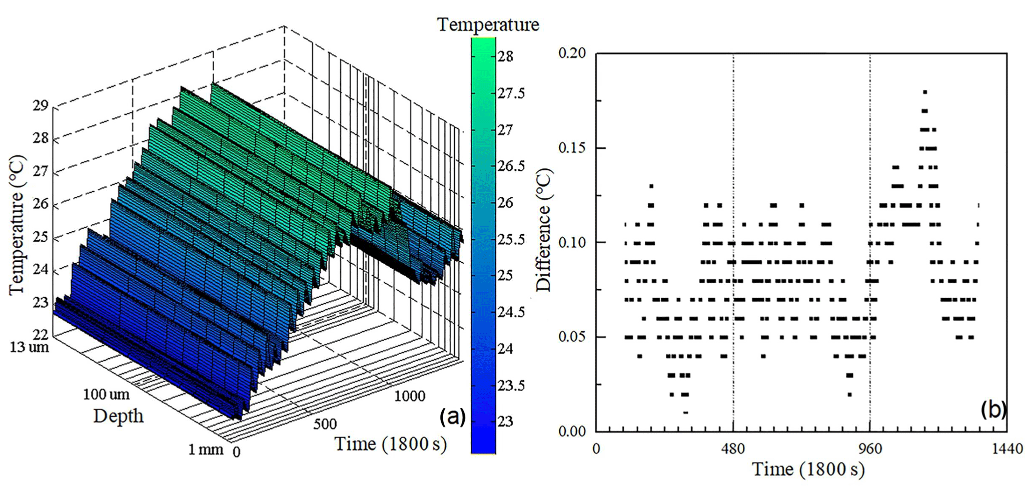
Figure 4SST depth changes simulated by the GOTM every half hour for a pixel with a longitude of 32.65∘ and a latitude of 43.25∘ in July 2002 (panel a is the variation in ocean temperature at different depths; panel b is the difference between the sea surface skin temperature and sea surface subskin temperature).
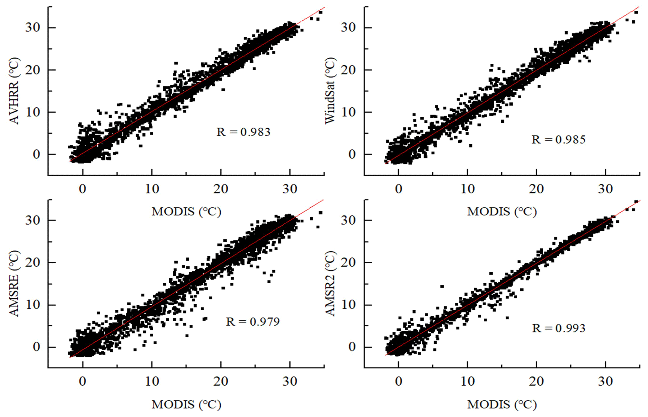
Figure 5Scatter diagrams of the MODIS SST data and ocean multisource data compensated for different measurement times and effective sampling depths.
3.1.2 Bias adjustment scheme for in situ observations
SSTs retrieved from MODIS sensors are skin SSTs. However, in situ SSTs from Version 2.1 NOAA iQuam are subsurface SSTs. For Argo floats, only the shallowest high-quality measurement is extracted and saved from each profile into the iQuam dataset (the same algorithms are used for other in situ platforms, such as those on ships, drifters, and moorings), along with its measurement depth. The closest measurement to the surface of the Argo float is at a depth of 3–8 dbar (0.15–0.2 m for drifters and ∼1 m for moorings). The differences between skin and subsurface SSTs, as described by Donlon et al. (2002), can be as large as 1.0–2.0 ∘C when the solar insolation is strong and the wind speed is weak. Figure 6 shows that the differences between the MODIS data and the eight types of in situ SSTs from iQuam can be significant under different weather conditions. When combining in situ SSTs into the MODIS SST product, such differences need to be accounted for. Therefore, in situ SSTs were first collocated and made coincident with MODIS data (within ±1 h and ±0.02∘ of latitude and longitude). Then, the coincident in situ SSTs were adjusted using the temperature depth and observation time correction model by entering the SST measurement depth and corresponding meteorological parameter values present during the measurement, including the wind speed at a 10 m height, the air temperature at a 2 m height above the sea surface, air humidity data, and cloud cover data from the ECMWF.
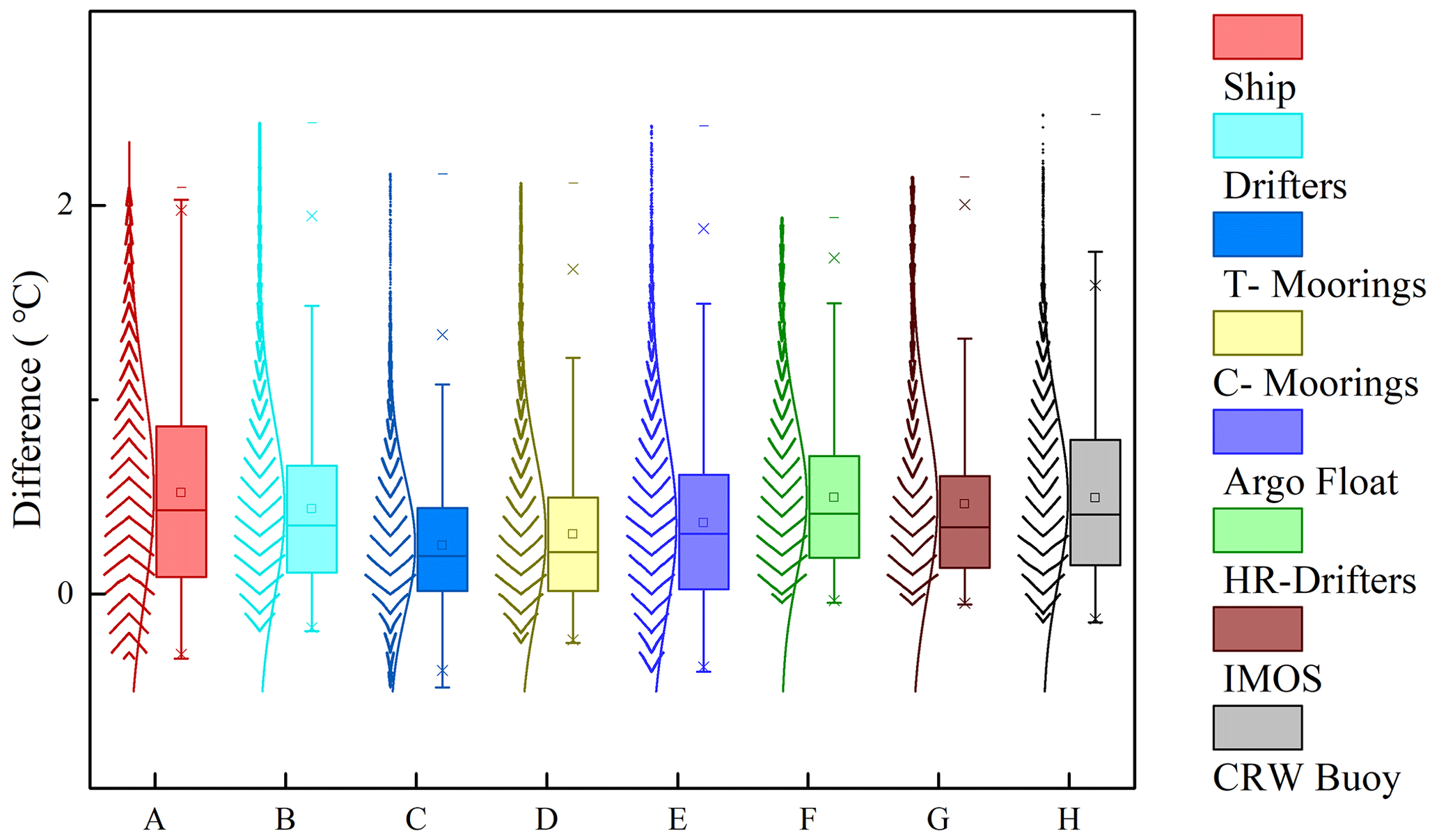
Figure 6Box chart with scatters representing the differences between the original MODIS data and eight types of in situ SST observations.
3.2 Filtering of MODIS SST
The monthly MODIS SST data cover the whole sea area of the world, but they contain many missing and low-quality pixels caused by factors such as clouds and aerosols. Figure 7 shows the frequency of non-null pixels, including valid pixels and low-quality pixels, in the monthly MODIS SST data from July 2002 to December 2019. The missing pixels are mainly distributed in high-latitude sea areas beyond ±60∘ of latitude. In the middle- and low-latitude sea areas within ±60∘ of latitude, the coverage rate of pixels is more than 95 %. There are many missing pixels distributed off the Peru coast, in the El Niño–Southern Oscillation (ENSO) signal region, due to the widespread low clouds over the eastern South Pacific off the coasts of Chile and Peru (Satyamurty and Rosa, 2020). In addition, there is a lower frequency of non-null pixels in the Inter-Tropical Convergence Zone (ITCZ) region and other tropical oceanic areas west of the continents due to the cloud cover in these areas (Ackerman et al., 2008; McCoy et al., 2017). In most areas of low and middle latitudes, the non-null pixel coverage is as high as 100 %, but it is difficult to detect the cold top surface of thin clouds or subpixel clouds, and the SSTs retrieved under such conditions are usually underestimated because the temperatures of clouds are almost always colder than the temperature of the sea surface (Reynolds et al., 2007). Moreover, other factors can also contaminate the observed signals and affect the data quality, such as factors related to the radiometer, including its viewing geometry, spectral response, and noise level (Kilpatrick et al., 2015). Therefore, there are many low-quality pixels among non-null pixels in the low and middle latitudes during the study period. In this study, the spatial process of the SST reconstruction includes the removal of low-quality pixels in low-latitude and midlatitude regions and the reconstruction of low-quality and missing pixels in the low-latitude and midlatitude regions and the high-latitude regions.
The quality control information stored in the qual_sst layer is provided along with the MODIS L3m SST data, with the quality level 0 being the best quality and the quality level 4 being the worst. These values can be found in the original MODIS SST netCDF files (see Sect. 2.1 for a detailed description). The missing pixels present in these data are represented by the filling value −32 767. Therefore, the quality control labels and the filling value were used to identify low-quality and missing pixels in the MODIS SST product. For monthly and daily SST data, to ensure the data quality and the number of effective pixels, pixels with a quality level ≤1 were considered to be high-quality data.
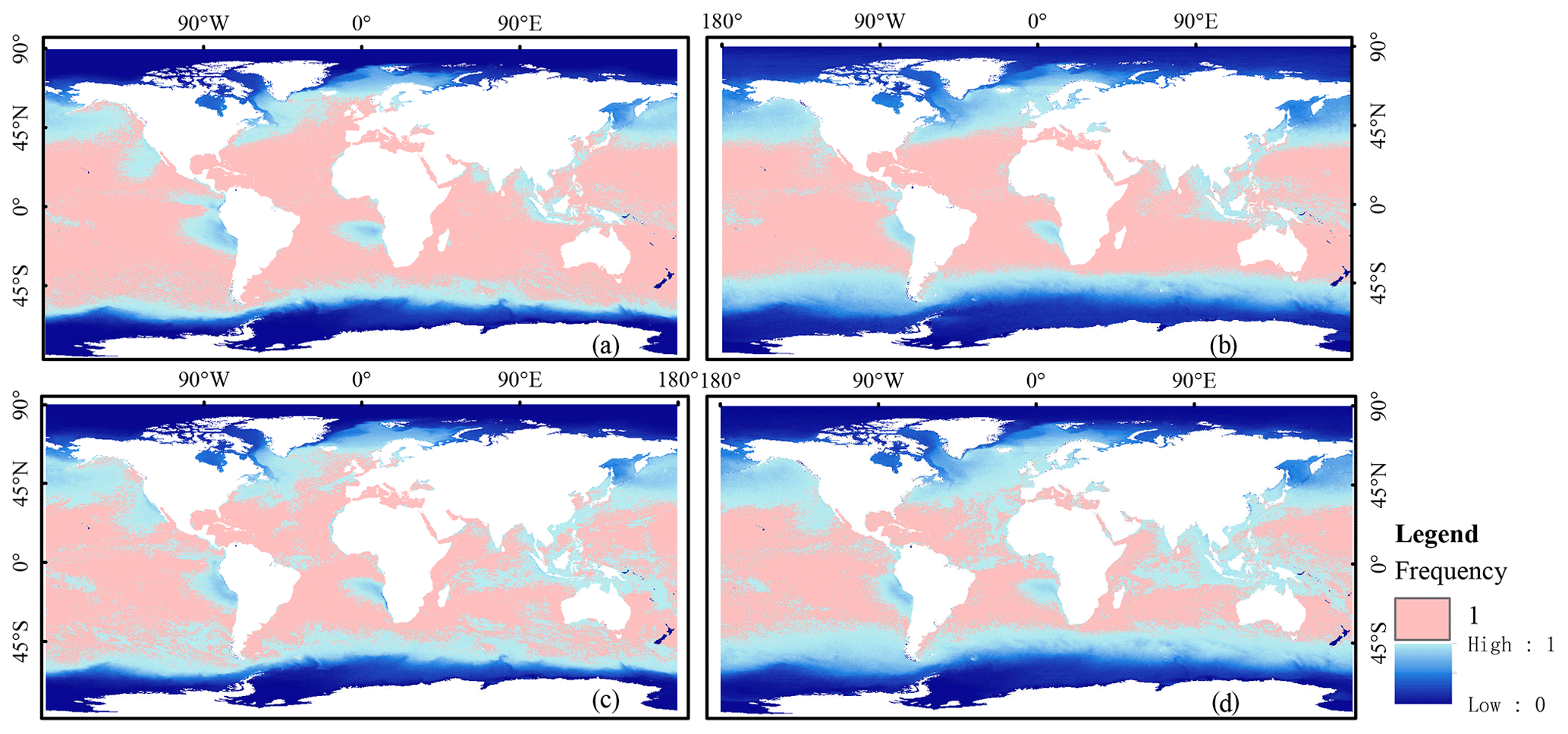
Figure 7Frequency of non-null pixels, including valid pixels and low-quality pixels, in the monthly MODIS SST data during the study period from (a) nighttime Aqua overpasses, (b) daytime Aqua overpasses, (c) nighttime Terra overpasses, and (d) daytime Terra overpasses.
3.3 SST data reconstruction
In the data processing, we first filtered all input monthly MODIS SST images and determined the locations of the low-quality and missing pixels. Then, for each invalid pixel (i.e., the low-quality and missing pixels) in the monthly images, we filtered the daily MODIS SST data of the respective month at the corresponding location. The high-quality pixels in the daily SST data were retained, and the invalid pixels in the daily data were reconstructed by combining multisource data. Finally, the invalid pixels present in the monthly data were replaced by the mean SST values derived from the gap-filled daily SST time series of the corresponding month. Combining the characteristics of multisource data and the availability of the data, we adopted different methods to reconstruct the invalid pixels present in the daily MODIS SST data for different regions.
3.3.1 Reconstruction of invalid SST pixels in low-latitude and midlatitude marginal regions of the ocean
Due to the influence of the mixed pixels in adjacent coastal areas, sea surface temperature products obtained from passive microwave remote sensing have very large uncertainties in these areas (Xie et al., 2008), which result in more invalid or low-quality pixel values in adjacent coastal areas. Therefore, invalid pixels in these regions were first filled with in situ or AVHRR SST data, and these pixels filled with in situ observations were marked. Then, in cases where these observations were missing, we filled these invalid pixels based on the geographically weighted regression (GWR) and Kalman filtering (KF) methods, fitted the SSTs obtained by the two methods, and finally reconstructed the invalid pixels. A summary flow chart of the process is schematically illustrated in Fig. 8.
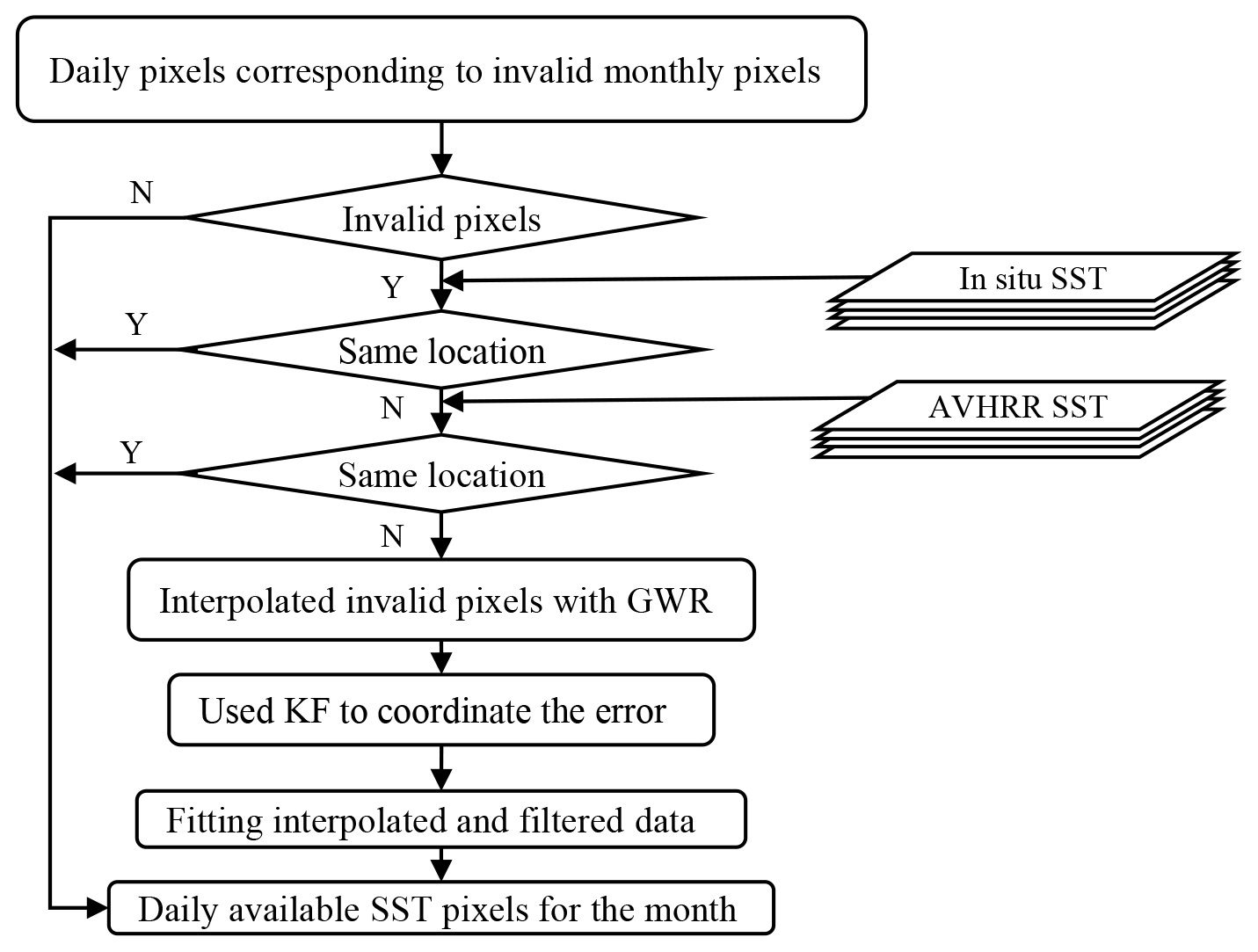
Figure 8A summary flow chart for reconstructing invalid SST pixels in low-latitude and midlatitude marginal regions of the ocean.
-
Interpolating invalid pixels with GWR.
GWR is an effective method for estimating missing pixels, which can quantitatively determine the contribution of adjacent pixels to contaminated pixels (Zhao et al., 2020). This method assumes that the spatially adjacent pixels with similar meteorological conditions have similar temperature values. Therefore, after determining the pixels, the GWR method was used to reconstruct invalid pixels. To determine the sliding window with the minimum noise and the best complement value, we simulated the size of the experimental pixel window many times and selected a sliding window of 15 by 15 pixels centered on the target pixel. This window size also avoids the reduction in execution efficiency caused by the redundancy of pixel involved in the calculation and ensures the number of pixel values involved in the calculation. During the reconstruction of invalid pixels, the regression weight coefficient of each adjacent pixel was determined by the Euclidean distance between that pixel and the target pixel. Simultaneously, considering that the available pixels obtained from in situ observations are more representative of the real SST under the cloud cover, we assigned a relative multiple weight to the marked in situ data according to GWR. By selecting some marked pixels as experimental values, it was found that the target pixels can be estimated accurately when Mg (Mg is the weighting coefficient of the in situ assigned pixels) was set to 3. The weighting coefficients of adjacent pixels can be determined by Eqs. (5) and (6). Then a local linear regression calculation was performed for each point in the window according to the sample weights. This regression calculation can be expressed as Eq. (7).
Here D is the distance from the adjacent pixel to the target pixel. (x, y) and (xt, yt) are the locations of the adjacent pixel and target pixel, respectively. i and j are the adjacent pixels used to estimate the SST of the invalid pixel. i is an adjacent pixel of high quality. j is a pixel assigned by in situ measurement. Wi and Wj are weight multipliers. m is the number of i. n is the number of j, and Mc and Mg represent the weighting coefficients of the high-quality pixels and in situ assignment pixels, respectively. Mc and Mg are set at 1 and 3, respectively. Tt is the filled SST value of the target pixel.
-
Using KF to coordinate the error.
For this region, on the basis of interpolation, KF can be used to coordinate the error characteristics of the SST variation and the error characteristics of the interpolation. Since the SST variation is relatively flat, SST is treated as a stationary random process. Due to the slowly changing characteristics of SST and the lack of effective temperature values representing these pixels, we took into account the SST data representing the adjacent time at the location of the invalid pixel. Considering the operational requirements of SST real-time retrievals and the necessary computing speed and storage capacity of the computer, the correlation of the error changes with each observation time was not considered in the actual operation process, and only the simple random error was used to simulate the changes in the process error and measurement error. By modeling the data, the equation of the state of the system can be written as follows.
where Xt is state to be estimated at time instant t. Xt−1 is the state vector of the process at time t. ∅ is the state transition matrix of the process from the state at t−1 to the state at t, which is assumed stationary over time, and Wt−1 represents the process noise, which is considered to be Gaussian, and its covariance is represented by Q. We take the KF of 124 MODIS SST images in July 2002 as an example. All data were arranged in chronological order, and the change of the SST in each pixel relative to the SST of the previous time was counted. Based on the statistical results of these images, the covariance was 3.115⋅I (I is the identity matrix). Consider the following measurement equation.
where Zt is the measurement of X at time instant t. H is the noiseless connection between the state vector and the measurement vector, which is assumed stationary over time. Vt represents the measurement noise, which is also considered to be Gaussian, and its covariance is represented by R. R can be obtained by comparing the measurement data with the verification data (Xu and Cheng, 2021). Then, the following KF formula was used to combine the input data to achieve the optimal output of the system, which operates in a prediction update. The prediction equations are responsible for projecting forward (in time) the current state and error covariance estimates to obtain the a priori estimates for the next time step. The update equations are responsible for the feedback, i.e., for incorporating a new measurement into the a priori estimate to obtain an improved a posteriori estimate. Prediction equations are as Eqs. (10) and (11).
Update equations are as Eqs. (12), (13), and (14).
Here X, ∅, H, Q, and R can be obtained according to the explanation of Eqs. (8) and (9). K is the Kalman gain. P is the error covariance matrix.
-
Fitting interpolated and filtered data.
To more accurately reconstruct the pixels that lack valid observations, a data fitting shown in Eq. (15) was performed for the interpolated and filtered data, which are the SSTs obtained based on the GWR and the KF methods, respectively. Finally, the reconstruction of invalid pixels without in situ or AVHRR SST filling could be realized by using the data fitting.
where T′ is the reconstructed SST. Tg and Tk are the SSTs obtained based on the GWR and the KF methods, respectively.
To determine the best fitting parameters of α and β, we selected some valid pixels from each image and then interpolated and filtered these pixels. The Eq. (15) was used to fit the interpolated and filtered results, and the fitting coefficients of each SST image were obtained using the least-squares method.
where Ti is the valid pixel value in the image and n is the number of these pixels. When ΔT reaches a minimum value, the fitting coefficient can be obtained by using Eqs. (17) and (18).
3.3.2 Reconstruction of invalid SST pixels in low-latitude and midlatitude inner ocean areas
Similar to the method used to reconstruct invalid SST pixels in the marginal regions of the oceans at low and middle latitudes, pixels with invalid SST values were reconstructed through collocating with in situ and AVHRR data in inner ocean areas. The invalid pixels were filled using values from valid in situ SST or AVHRR data collected at the same location at the same time. In cases of missing in situ SST or AVHRR data, the SST was retrieved from passive microwave data to reconstruct the invalid SST data. A summary flow chart of the process is schematically illustrated in Fig. 9.
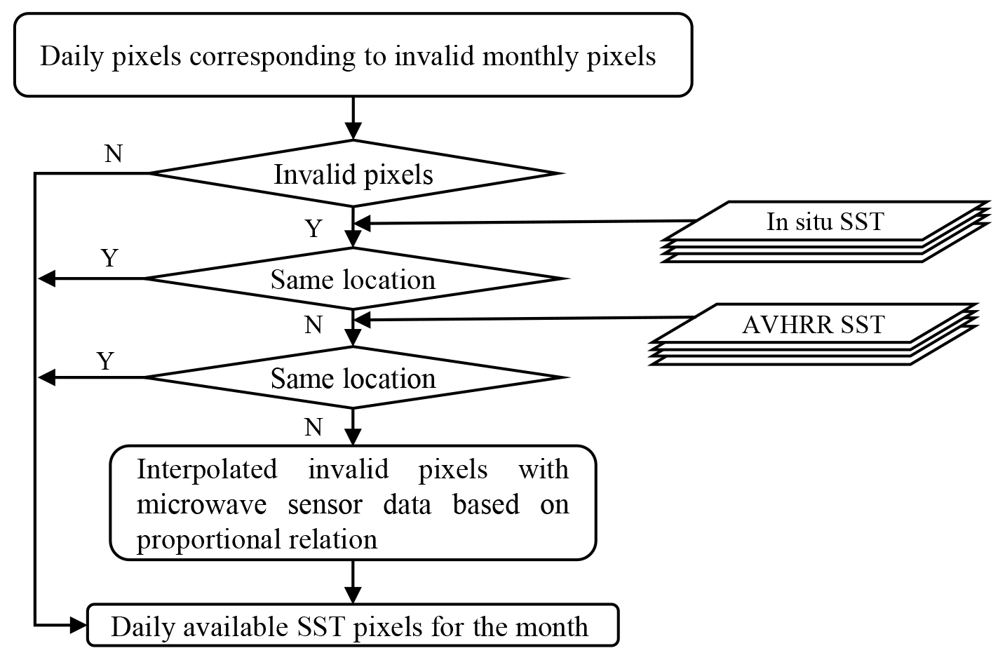
Figure 9The summary flow chart for reconstructing invalid SST pixels in low-latitude and midlatitude inner ocean areas.
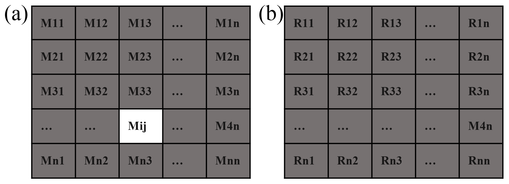
The temperature variation trends present in the MODIS daily data and microwave daily data on corresponding date in the same region are the same, so the two groups of data have the same proportional relation. Taking a grid of n pixels by n pixels as an example, a and b are considered the same regions clipped from the MODIS and microwave-based data, respectively. The gray and white rasters represent the effective and invalid pixels, respectively. Mkl and Rkl represent the pixel values of the MODIS and microwave-based data, respectively. K and L represent the pixel positions. Mij represents the value after the interpolation of invalid pixels.
The reconstruction of invalid pixels can be achieved by using the above formula. The reconstructed pixels meet the accuracy of the interpolated images to a certain extent and do not damage the original SST variation trend. After several simulations of different experimental pixel window sizes, the noise was found to be minimized when a sliding window of 6 by 6 pixels was used, and this window size was considered to have the best complement value.
3.3.3 Reconstruction of invalid SST pixels in high-latitude regions of the ocean
At high latitudes, sea ice covers a significant fraction of the global oceans (approximately 5 %–8 %). The presence of large areas of mixed sea ice and open water makes it difficult to retrieve SSTs (Høyer et al., 2012; Vincent et al., 2008). In addition, there is persistent cloud cover in polar regions, with cloud cover occurring up to 90 % of the time in summer and 50 %–60 % of the time in winter in the Arctic (Høyer et al., 2012). The continuous cloud cover and extended twilight period complicate the detection of cloud, which thus presents problems for identifying clouds correctly with cloud detection algorithms. Therefore, it is challenging to use satellite sensors to accurately retrieve SST at high latitudes, including the Arctic Ocean. Moreover, because of the existence of sea ice and the difficulty of navigating in ice-filled water, the number of field observations at the area is generally scarce compared to other regions (Reynolds et al., 2002). The Microwave and AVHRR SST data used in this study have limited available pixels in high-latitude regions, so it is impossible to reconstruct MODIS SST data in high-latitude regions only by relying on these data and in situ data.
High-latitude SSTs can be estimated based on satellite sea ice concentrations (SICs). In areas with sea ice, the SST is the temperature of the open water or of the water under the ice (Banzon et al., 2020). Multiple analysis (L4) products from GHRSST enable SST estimation near the polar region by converting SIC into SST. Due to differences in satellite source data, integration methods and methods for converting SIC to SST, the accuracy of level-4 SST products of GHRSST-PP varies in many aspects. After understanding the differences among current GHRSST level-4 products and their qualities and availabilities in different areas, the OISST V2.1 product was selected to restore invalid pixels in the MODIS SST data in the high-latitude area with sea ice coverage. In the product, SICs were revised to SSTs to remove warm biases in the Arctic region.
In areas of high latitudes, since the microwave-based SST data (used in this paper) exclude sea ice pixels, that is, SSTs are missing when the number of pixels with sea ice contamination exceeds a specified value, we used a combination of two strategies to reconstruct the missing SST data to improve the accuracy of the results. A summary flow chart of the process is schematically illustrated in Fig. 11.
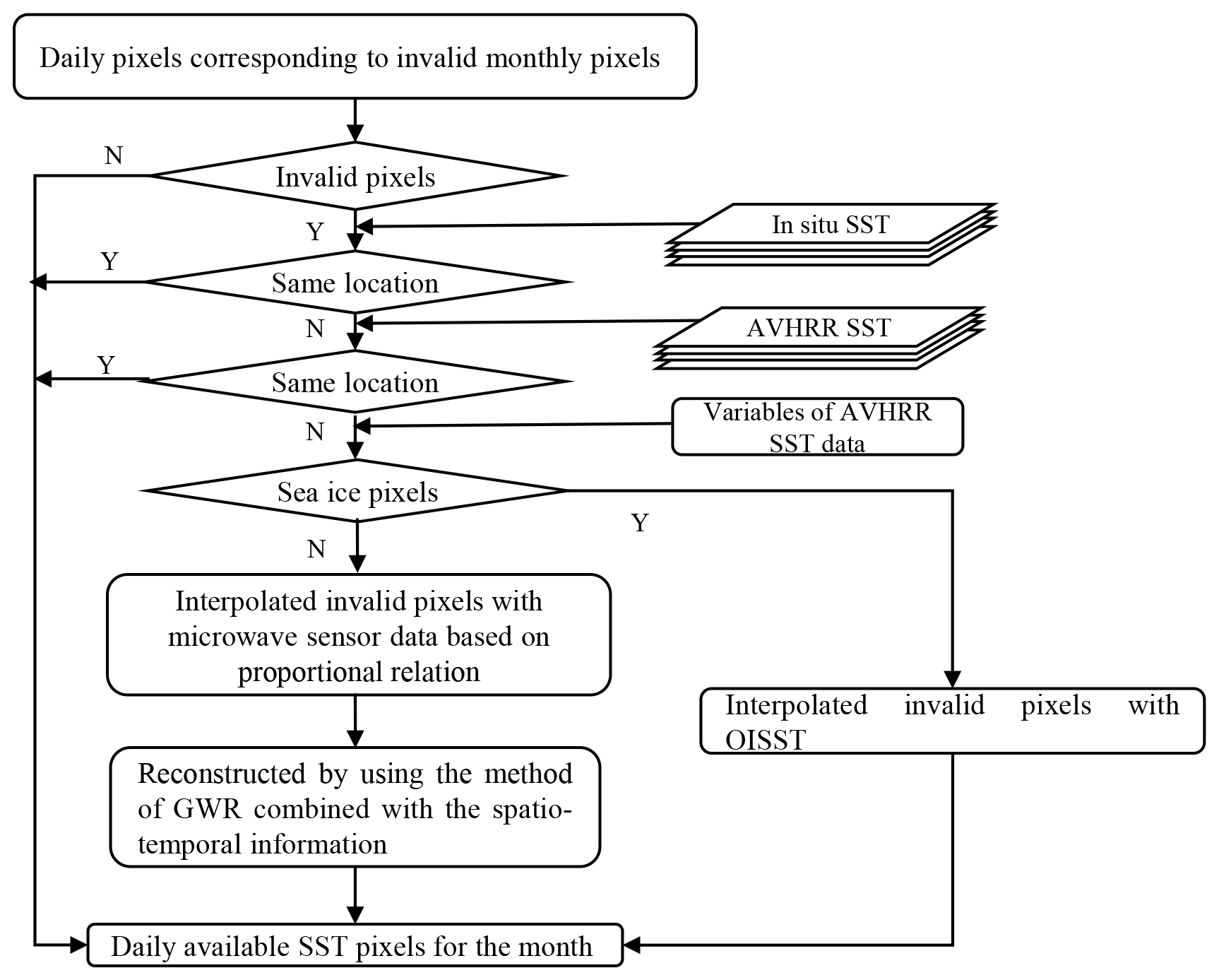
Figure 11The summary flow chart for reconstructing invalid SST pixels in high-latitude regions of the ocean.
First, the variables l2p_ flags and the sea ice fraction in the AVHRR SST data were used to identify the sea ice extent. The sea ice fraction variable quantified the fraction of sea ice contamination in a given pixel (ranging from 0 to 1), and bit 2 of the l2p_ flags variable was recorded if an input pixel recorded ice contamination. These variables can be used to identify sea ice pixels. Then, we used the first strategy to reconstruct invalid pixels in high latitudes without sea ice coverage. Pixels with invalid SST values in the MODIS data were collocated with in situ and AVHRR observations. Invalid pixels were filled using the values from the valid in situ or AVHRR data at the same location and the same time (priority was given to the use of in situ data). Then, for the invalid pixels without available observations, we used the method described in Sect. 3.3.2 above to fill the pixels using microwave data. Finally, considering the characteristics of the slow changes in SST and the fact that SST changes in the same area are interannual and its changes in the short term are usually small, the invalid pixels without any filling data were reconstructed by using the GWR method combined with spatiotemporal information. That is, we replace invalid pixels with the average value of valid pixels from the adjacent dates. If the number of effective pixels was too small, then the GWR method was used to reconstruct the invalid pixel. In another strategy, pixels with invalid SST values due to sea-ice-covered areas were collocated with in situ and AVHRR SSTs, which were filled using values from valid in situ SST or AVHRR data observed at the same location and at the same time. Finally, the adjusted OISST V2.1 products were used to reconstruct the invalid pixels when there are not sufficient replacement pixels in sea-ice-covered areas. The adjustment algorithm is a linear regression algorithm that relies on coefficients derived from co-temporal OISST and MODIS SST observations.
where TM is the adjusted SST. TO is the pixel value of the OISST product. α is the regression coefficient, which is determined by matching the data of the MODIS SST data and the OISST data, and β is the estimated intercept.
MODIS has superior coverage and performance in sampling global SST and has been verified by various studies (Barton and Pearce, 2006). Moreover, to better assess the accuracy of the new SST product, we performed verification of the original MODIS data, oceanic multisource data compensated for different measurement times and effective sampling depths, and the new SST data in different regions. The accuracy of the data was assessed using five statistical indexes: coefficient of determination (R2), root-mean-squared error (RMSE), bias, absolute bias (Abs_Bias), and scatter index (SI). The bias was calculated as the SST obtained from the MODIS product minus the in situ SST. The scatter index, usually denoted as SI, was used to measure the magnitude of the bias between the SST product and the in situ observations versus the in situ observations. A smaller SI means a more accurate measurement.
Here SSTi is the MODIS SST value of matching point i. is in situ observation value of matching point i. n is the number of matching points. and are the average value of SST obtained from MODIS products and the average value of SST obtained from in situ observations, respectively.
In addition, to convey information more easily and concisely, Taylor diagrams (Taylor, 2001) were also used to compare the accuracies of different SST products, as they provide a way to graphically summarize the relative accuracies of several products. Taylor diagrams are two-dimensional scatter plots in which discrete points give an indication of how well patterns match each other in terms of their correlation coefficient (R), centered RMSE (E), and normalized standard deviation (SDV), all at once (Castro et al., 2016). These statistics are defined as follows, where m and o are the simulated and observed patterns, respectively.
In the Taylor diagram, SDV is shown as the radial distance, and R is shown as the cosine of an azimuthal angle in the polar plot. The observed patterns are represented by points on the x axis at R=1 and SDV =1. E is the distance from the simulated patterns to the observed patterns, and this distance can quantify how closely the simulated patterns resemble the observed patterns.
4.1 Evaluation of the original product
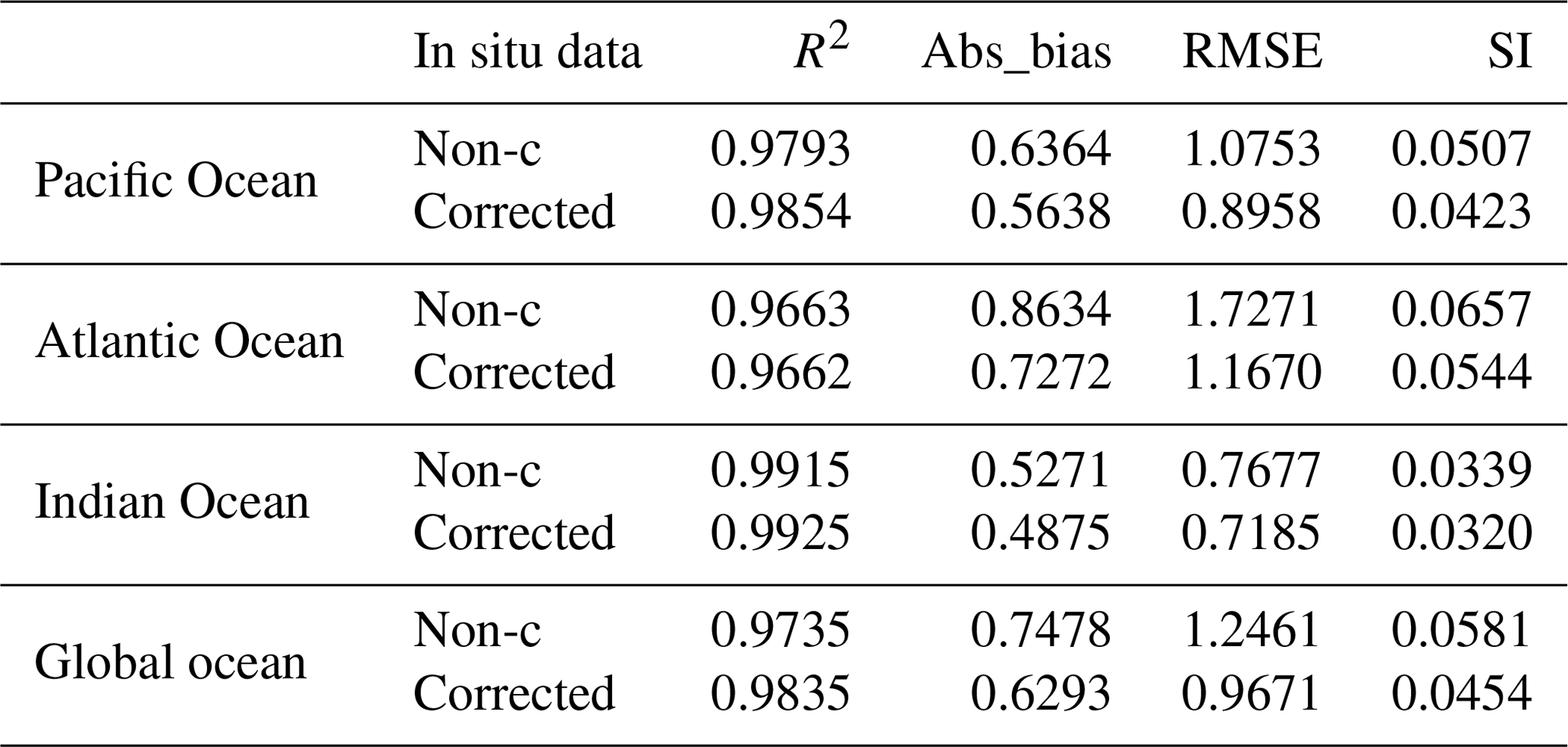
We conducted a comparative analysis based on the distribution of invalid pixels in different regions, and the validations of the original monthly MODIS SST values against in situ SST measurements (including the uncorrected in situ data and corrected in situ data) were shown in Table 1. Validation using in situ SST measurements shows that the RMSE ranges from 0.768 to 1.727 ∘C (SI: 0.034–0.066), and validation using corrected in situ SST measurements indicates that the RMSE ranges from 0.719 to 1.167 ∘C (SI: 0.032 to 0.544).
Table 1Statistics of the validation results of original monthly MODIS SSTs against in situ SST measurements (non-corrected/corrected).
4.2 Evaluation of the bias adjustment
4.2.1 Evaluation of satellite data bias adjustment
Different sensors and satellites can obtain measurements at several different times throughout the diurnal cycle. In addition, microwave and thermal infrared sensors have different effective measurement depths. Since both the AMSR-E and MODIS instruments are aboard the Aqua satellite, they both pass through the Equator at approximately 01:30 and 13:30. Therefore, in order to verify the depth correction model, we used the depth correction model to perform depth correction on the daily AMSR-E data. That is, the sampling depth of AMSR-E daily data was corrected to the sampling depth of MODIS data, and then the corrected values were compared with the corresponding MODIS daily data. Figure 12a shows the validation results of the AMSR-E SST data, which show that the overall result between the corrected data and the MODIS data presents a good linear relationship. The RMSE is reduced from 1.137 to 0.508∘, and the absolute bias is reduced from 0.718 to 0.302∘, which indicates that the model can simulate the SST at different depths well. Furthermore, we compared and analyzed the nighttime products of the same sensor with the corresponding daytime products after a time correction to verify the time correction performed by the model. Taking AMSR-E daytime SST products as an example, we corrected these SST values to the corresponding nighttime SST values (Fig. 12b). Shown from Fig. 12b, there was an obvious diurnal warming before the correction, and the data after the correction had lower absolute bias and RMSE values. Thus, the model can also simulate the diurnal variation in the SST well and can be used to normalize the SSTs observed at different times.
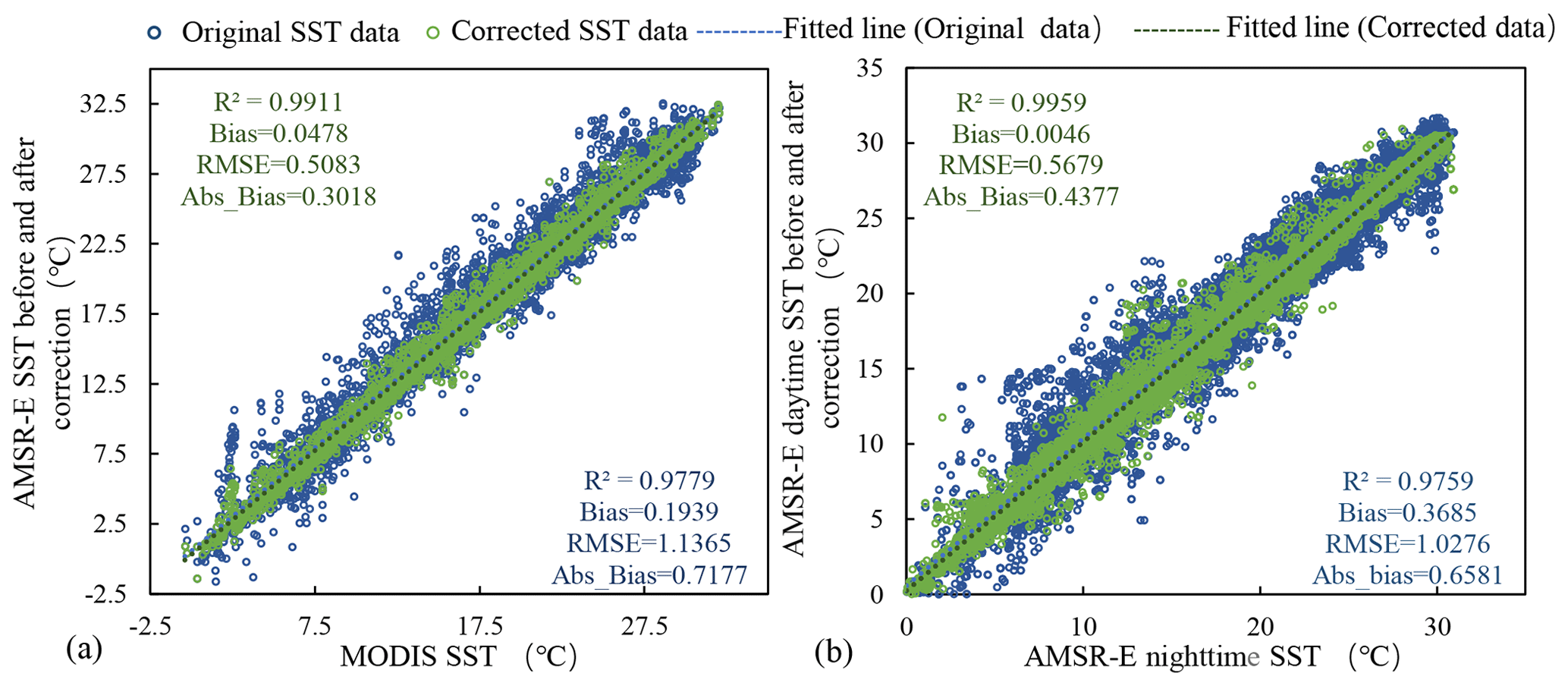
Figure 12The scatter diagrams of the daily original SST data and corrected results versus their corresponding actual SST data from 2002 to 2019. The blue points indicate original SST pixel values. The green points represent the values in corrected SST data, and the statistical accuracy measures (R2, bias, Abs_Bias, and RMSE) are also indicated.
4.2.2 Evaluation of in situ data bias adjustment
To validate the correction results of the temperature depth and observation time correction model on in situ SSTs, we selected the matchups corresponding to the effective pixels of daily MODIS SSTs from in situ SSTs and compared and analyzed the daily MODIS SSTs with these matchups. Figures 13 and 14 both show the verification results of the MODIS SSTs against in situ data before and after the calibration. Figure 13 reflects the change in the difference between all types of in situ data before and after the correction and the corresponding MODIS SST data. It can be shown from Fig. 13 that the range of temperature difference between uncorrected in situ data and MODIS data is about −2–2.5∘, while the difference range between corrected in situ data and MODIS data is reduced to the range of −0.5–0.75∘. Figure 14 is based on the MODIS SST data as a reference and shows the distribution of SSTs before and after the correction from the eight platforms described in the normalized Taylor diagram. In Fig. 14, the degrees of agreement are compared among in situ data from different platforms before and after the correction with the MODIS data. The points representing in situ SSTs lying near the MODIS observations (the MODIS observations are represented by points on the x axis at R=1 and SDV =1) have relatively high R and low E values. After the correction, the points representing in situ SSTs are closer to the MODIS observations, which means that compared with in situ data before correction, the agreement between the two is better. Therefore, the corrected result of the model is stable and reliable and can be used for the conversion of SSTs from in situ observations taken at different depths.
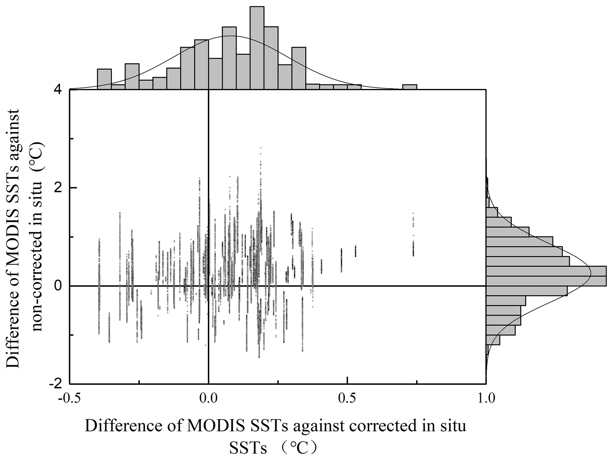
Figure 13Marginal histogram of the difference between in situ data before and after correction and the corresponding MODIS SST data. (The margins of the scatterplot are a histogram of the variables, indicating the distribution of data in either direction.)

Figure 14Normalized Taylor diagrams showing differences between matched SST from in situ data before and after correction and the corresponding MODIS SST data.
4.3 Evaluation of the new product
4.3.1 Accuracy verification of low-quality pixels
In this study, we only restored invalid pixels, including low-quality pixels and missing pixels, in the MODIS data and first evaluated the improvement effect of these pixels. Figure 15 shows the validation results of the low-quality MODIS SST data and the reconstruction results versus the corresponding in situ observations, including the corrected in situ data and uncorrected in situ data. The validation results indicate that the reconstructed MODIS SST data are always more consistent with in situ data, including the corrected data and uncorrected data, than the values before reconstruction, with RMSE values lower than 0.675 ∘C and R2 values higher than 0.991. Compared with the original values, the accuracies of the corrected values are improved by more than 0.65 ∘C.
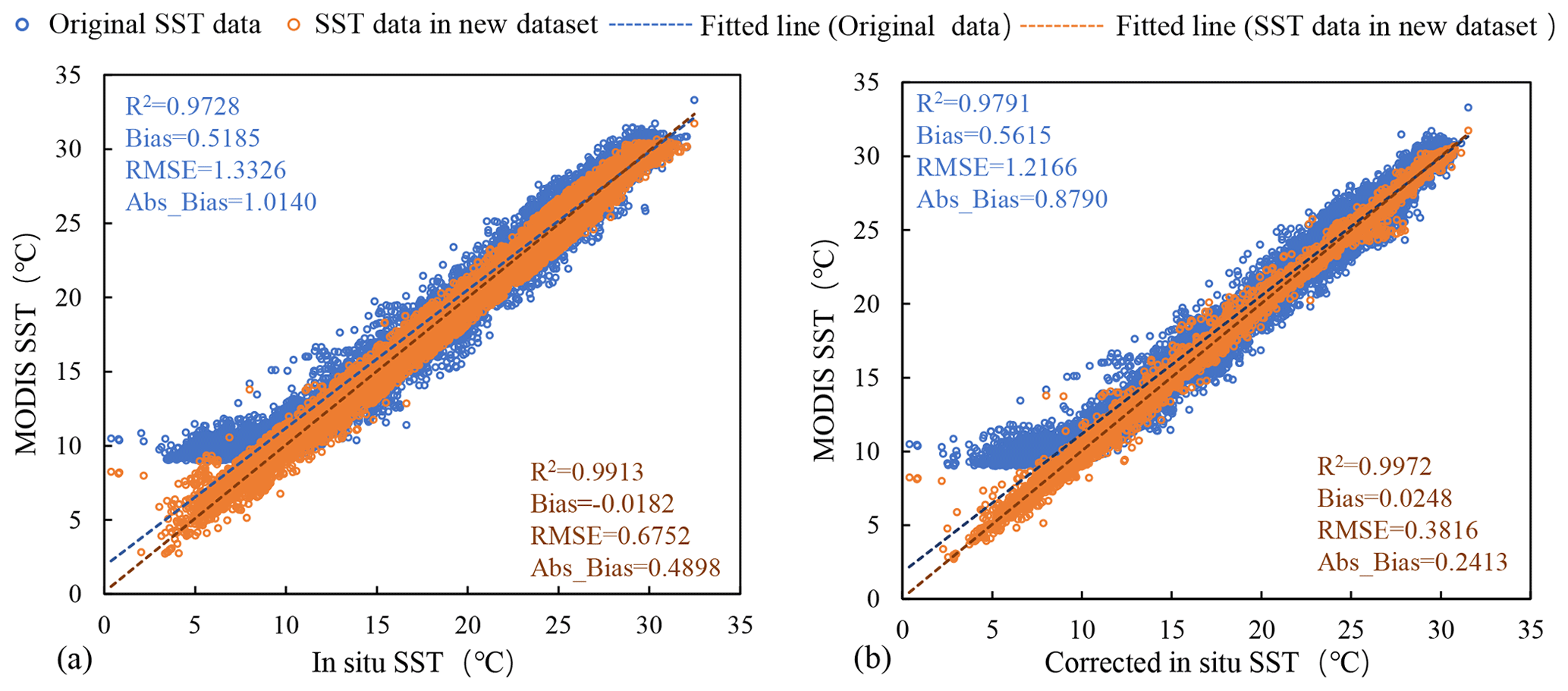
Figure 15The scatter diagrams of the low-quality MODIS SST data and the reconstruction results versus their corresponding in situ SST data from 2002 to 2019. The blue points indicate low-quality MODIS SST pixel values. The orange points represent the values in reconstructed SST data, and the statistical accuracy measures (R2, bias, Abs_Bias, and RMSE) are also indicated.
4.3.2 Overall accuracy verification
To fully verify the overall accuracy of the reconstructed SST products, we compared the performances of the original MODIS SST and the reconstructed SST products relative to in situ data via Taylor diagrams. The normalized Taylor diagrams showing the performances of the two products relative to in situ data before and after the correction are presented in Fig. 16. Compared with the original MODIS product, the reconstructed product can better represent the in situ observations, with the highest R value, lowest E value, and SDV closest to 1. Among them, the original MODIS product with the lowest consistency with both the uncorrected observations and the corrected observations by far consists of the Atlantic SSTs, with E=0.090 and 0.057, SDV =0.967 and 0.982, and R=0.954 and 0.9711, respectively. After reconstruction, the Atlantic SSTs show very good correlation, with a lower E value and SDV closer to 1 with both the corrected and uncorrected observations, and its accuracy is significantly improved.
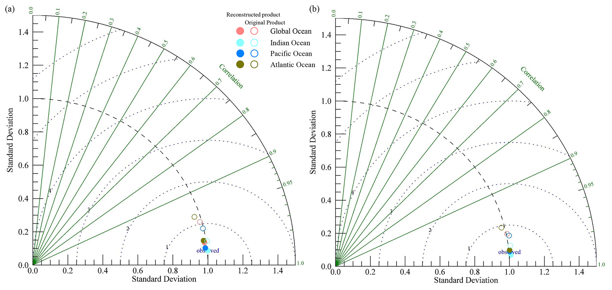
Figure 16Normalized Taylor diagrams showing differences between matched SST from in situ data before (a) and after (b) correction and the corresponding SST products.
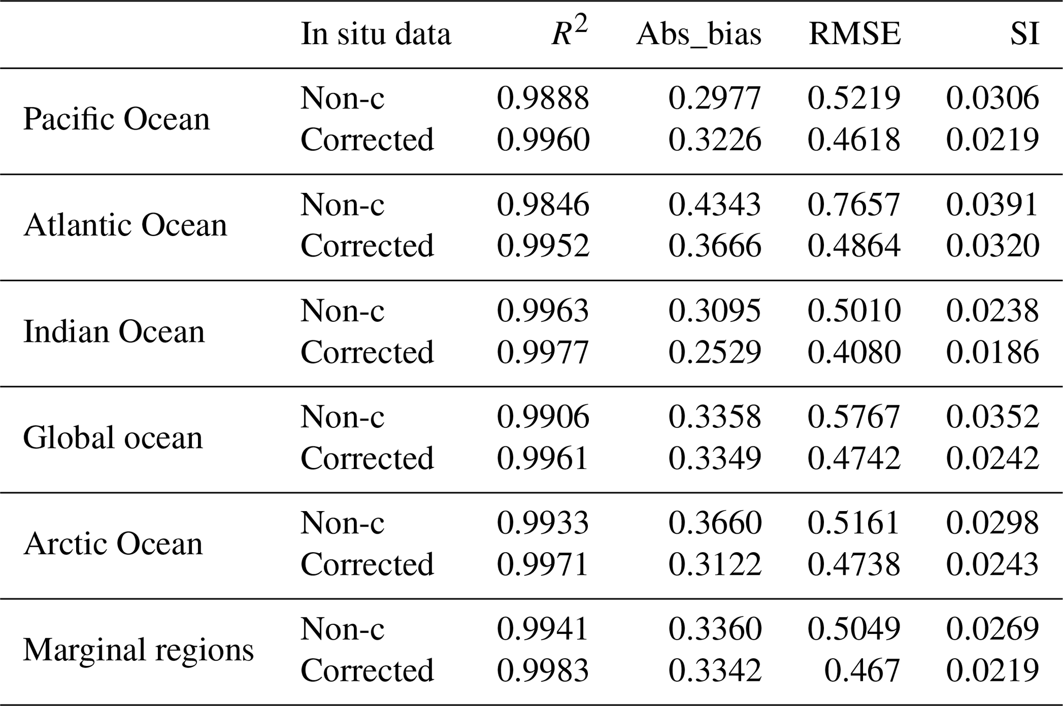
To further understand the credibility of the reconstructed product and clarify the limitations of this method, we further assessed the performance in terms of the output biases in different regions. The associated validation statistics of the new SST dataset against the corrected in situ observations and uncorrected in situ observations are summarized in Table 2. The new dataset is in agreement with the uncorrected in situ observations with abs_bias =0.3358 ∘C, RMSE =0.5767 ∘C, and SI =0.0352 on the global ocean. Among these statistics, the RMSE, SI, and abs_bias of the Atlantic region are slightly larger than the values in the global ocean, but they are all better than those of the original MODIS SST data (see Table 1 for details), the correlation coefficients of this product in different regions are all greater than 0.984, and these SI values are less than 0.04. For the whole ocean, the abs_bias of the new SST product relative to the corrected in situ observations is 0.3349 ∘C, and the RMSE and SI are 0.4742 ∘C and 0.0242, respectively. The RMSE, SI, and abs_bias of the values of the Atlantic Ocean region are also slightly larger than those of the global values. However, they are still better than those of the original MODIS SST data (see Table 1 for details), the correlation coefficients of the product in the different areas are greater than 0.995, and these SI values less than 0.032. In addition, the RMSE and SI values of the edge areas and high-latitude areas are slightly lower than the global values, which indicates that the accuracy of the data in these areas is higher. These results indicate that the reconstructed MODIS SST dataset is robust and accurate due to its high consistency with in situ observations, including corrected and uncorrected observations. Therefore, we believe that the accuracy of SST data can be improved by the method adopted in this paper.
Table 2Statistics of the validation results of new SSTs against in situ SST measurements (non- corrected/corrected).
To investigate the performance of the reconstructed product relative to the other products, a comparison between the OISST product and the reconstructed data was conducted during 2002–2019. OISST Version 2.1 is an analysis product constructed by combining observations from different platforms on a regular global grid, such as AVHRR data from NOAA satellites, ships, Argo floats, and drift floats, with a spatial grid size of 0.25∘. For the OISST images, we averaged the daily SST data corresponding to each month and obtained monthly SST images. Then, the dataset was validated against the corresponding in situ observations, including the uncorrected and corrected in situ SSTs, as shown in Fig. 17a. The RMSE values of OISST against the uncorrected and corrected in situ observations in the global ocean were 0.602 and 0.495 ∘C, respectively. Those of the reconstructed SSTs against the uncorrected and corrected in situ observations in the global ocean were 0.577 and 0.474 ∘C, respectively. Compared to these, the overall accuracy of the reconstructed data is better. In addition, we also performed an intercomparison with the 2∘ Extended Reconstructed Sea Surface Temperature (ERSST) product, which is a global monthly SST dataset derived from the International Comprehensive Ocean–Atmosphere Dataset (ICOADS) that uses statistical methods to enhance spatial completeness. Figure 17b reflects the monthly average SST changes in different oceans from the ERSST product and the reconstructed products over the 2002–2019 period, indicating a reasonable consistency between the two. Based on the accuracy assessment and data intercomparison results, it can be seen that the reconstructed MODIS products of 2002–2019 are reliable with high accuracies and that the reconstructed models we designed are effective.
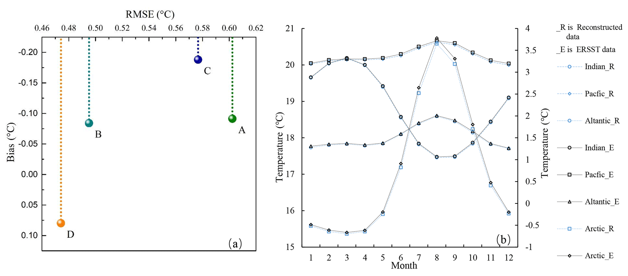
Figure 17Validation statistics of the reconstructed product and other SST products during 2002–2019. (a) Intercomparison with OISST, where A and C represent the results of OISST and new SSTs against uncorrected in situ SST measurements, respectively. B and D represent the results of OISST and new SSTs against corrected in situ SST measurements, respectively. (b) Intercomparison with ERSST, where black and blue are monthly mean SST changes of ERSST and new SSTs in different ocean from 2002 to 2019.
Bias adjustment was conducted with GOTM version 5.2.1 and is available at https://github.com/gotm-model/code/tree/v5.2 (last access: 24 August 2019). The code for data processing can be downloaded at https://doi.org/10.5281/zenodo.4762067 (Cao et al., 2021b).
The reconstructed MODIS SST products at 0.041∘ resolution from 2002 to 2019 are freely available to the public in the img format at https://doi.org/10.5281/zenodo.4419804 (Cao et al., 2021a), which are distributed under a Creative Commons Attribution 4.0 License.
The purpose of this study is to build a long-term series of global major meteorological disaster remote sensing datasets with high spatiotemporal and consistency based on the current global multi-source remote sensing data and ground observation site data and to provide key ocean temperature parameters (such as sea surface temperature) for marine meteorological disaster forecasting models, especially rapid forecasts of marine disasters such as typhoons, and provide early warning services for global fishing vessels and merchant ships.
In order to ensure the temporal and spatial consistency of different data, we built a GOTM based on temperature depth and observation time correction for modeling of the diurnal signal at different depths, thus bridging the gap of multi-source data. The GOTM model simulates the hydrodynamic and thermodynamic processes of vertical mixing of one-dimensional water columns in natural waters, and comprehensively considers the effects of solar shortwave radiation, longwave radiation, latent heat, sensible heat and cloudiness on the diurnal variations in SST, which can more accurately simulate the diurnal variations in SST than traditional empirical regression models that only consider the main factors of diurnal variations (such as wind speed, solar radiation, etc.). In addition, it has a high vertical resolution and can be encrypted on the surface layer to simulate the difference between the skin layer and the sub-skin layer, so as to achieve the uniformity of temperature at different observation depths. Therefore, the method-based GOTM simulation was used to unify the temporal and spatial reference of SST at different depths and different times for each pixel of the image, and the accuracies of each sensor and in situ observations are improved about 0.3–0.8∘. However, there are still certain errors, which are related not only to the characteristics of different sensors, retrieval algorithms, etc., but also to the accuracy of the GOTM model simulation. The simulation accuracy of GOTM largely depends on the input meteorological parameters. The wind speed, sea temperature, relative humidity, cloud cover, and other data used in this paper come from ECMWF reanalysis and forecast data. The spatial resolutions of these data are relatively low, which has some influence on accuracy. If the meteorological parameters with higher accuracy and resolution are available, the simulation accuracy can be improved further. In addition, when correcting temperature obtained from in situ observations, not every in situ observation from iQuam records the depth at the same time. For example, the actual temperature measured by the drifting buoys is not fixed at 0.2 m beneath the surface, which will fluctuate due to the influence of waves and other factors. Therefore, there will be a certain deviation in the correction of the skin layer, and these factors will ultimately affect the accuracy of the reconstructed product.
In addition, the SST data in the grid form represent the average temperature in the grid area, while in situ observations represent just the temperature near the locations of the stations. Although the study used the average value of the high-quality observation data that fall in the grid area with temporal sampling less than or equal to 1 h as the matched data of the grid, it was still limited by the number of measured data within the grid. Especially in the high-latitude areas where the measured points are sparse, the uncertainties associated with such matches could potentially bias the reconstruction and validation results. Therefore, more meteorological observation stations are needed to help improve the accuracy of the product. The acquisition and integration of rasterized SST are a complex problem, and the reconstruction models proposed in this research are just the beginning, which needs to be improved and developed continuously. Better solving the time phase and sampling depth problems of satellite remote sensing data and to introducing multiple types of data sources into the model are ways to improve the product accuracy.
Finally, a new SST product was obtained with high spatiotemporal coverage based on multisource data after calibration by using the above model. The product, generated by inputting infrared-based, microwave-based, and in situ SST data into the reconstruction spatial model, has a monthly temporal interval and a 0.041∘ spatial interval, which has higher accuracy and better consistency with statistics than the original datasets, and it combines the advantages of multi-source data. Detailed comparisons and analyses with OISST and ERSST products also illustrate the reliability and accuracy of the reconstructed product. Thus, this product can be used for mesoscale ocean phenomenon analyses. It will be useful in research related to global change and local area disaster prevention and mitigation. In addition, the reconstruction strategy used in this study can be extended to other multi-source and multi-temporal satellite data space-time gapless field reconstruction.
MC and KM designed the research and developed the methodology; MC wrote the manuscript; and KM, YY, and all other authors revised the manuscript.
The authors declare that they have no conflict of interest.
The authors would like to thank the National Aeronautics and Space Administration (NASA), the NOAA National Centers for Environmental Information, the Naval Research Laboratory (NRL) Remote Sensing Division and the Naval Center for Space Technology, and other agencies for their support by providing the SST product. We also thank the ECMWF for providing the climate reanalysis data.
This work was supported by the National Natural Science Foundation of China (grant no. 41921001), National Key Project of China (grant nos. 2018YFC1506502 and 2018YFC1506602), Fundamental Research Funds for Central Non-profit Scientific Institution (grant no. 1610132020014), and Open Fund of State Key Laboratory of Remote Sensing Science (grant no. ofSLRSS201910).
This paper was edited by Giuseppe M. R. Manzella and reviewed by Prakki Satyamurty and one anonymous referee.
Ackerman, S. A., Holz, R. E., Frey, R., Eloranta, E. W., Maddux, B. C., and McGill, M.: Cloud detection with MODIS. Part ii: validation, J. Atmos. Ocean. Tech., 25, 1073–1086, https://doi.org/10.1175/2007JTECHA1053.1, 2008.
Alerskans, E., Høyer, J. L., Gentemann, C. L., Pedersen, L. T., Nielsen-Englyst, P., and Donlon, C.: Construction of a climate data record of sea surface temperature from passive microwave measurements, Remote Sens. Environ., 236, 11485, https://doi.org/10.1016/j.rse.2019.111485, 2020.
Banzon, V., Smith, T. M., Steele, M., Huang, B., and Zhang, H.-M.: Improved estimation of proxy sea surface temperature in the Arctic, J. Atmos. Ocean. Tech., 37, 341–349, https://doi.org/10.1175/jtech-d-19-0177.1, 2020.
Banzon, V. F. and Reynolds, R. W.: Use of windsat to extend a microwave-based daily optimum interpolation sea surface temperature time series, J. Climate, 26, 2557–2562, https://doi.org/10.1175/jcli-d-12-00628.1, 2013.
Barton, I. and Pearce, A.: Validation of GLI and other satellite-derived sea surface temperatures using data from the Rottnest Island ferry, Western Australia, J. Oceanogr., 62, 303–310, https://doi.org/10.1007/s10872-006-0055-5, 2006.
Benali, A., Carvalho, A. C., Nunes, J. P., Carvalhais, N., and Santos, A.: Estimating air surface temperature in Portugal using MODIS LST data, Remote Sens. Environ., 124, 108–121, https://doi.org/10.1016/j.rse.2012.04.024, 2012.
Bretherton, F. P., Davis, R. E., and Fandry, C. B.: A technique for objective analysis and design of oceanographic experiments applied to MODE-73, Deep-Sea Res. Oceanogr. Abstr., 23, 559–582, https://doi.org/10.1016/0011-7471(76)90001-2, 1976.
Burnett, W., Harper, S., Preller, R., Jacobs, G., and LaCroix, K.: Overview of operational ocean forecasting in the US navy past, present, and future, Oceanography, 27, 24–31, https://doi.org/10.5670/oceanog.2014.65, 2014.
Cao, M., Mao, K., Yan, Y., Shi, J., Wang, H., Xu, T., Fang, S., and Yuan, Z.: A new global gridded sea surface temperature data product based on multisource data (Version 1.0) [Dataset], Zenodo, https://doi.org/10.5281/zenodo.4419804, 2021a.
Cao, M., Mao, K., Yan, Y., Shi, J., Wang, H., Xu, T., Fang, S., and Yuan, Z.: A New Global Gridded Sea Surface Temperature Data Product Based on Multisource Data (Version 1.0) [Code], Zenodo, https://doi.org/10.5281/zenodo.4762067, 2021b.
Carton, J. A. and Giese, B. S.: A Reanalysis of Ocean Climate Using Simple Ocean Data Assimilation (SODA), Mon. Weather Rev., 136, 2999–3017, https://doi.org/10.1175/2007mwr1978.1, 2008.
Carton, J. A., Chepurin, G. A., and Chen, L.: SODA3: A new ocean climate reanalysis, J. Climate, 31, 6967–6983, https://doi.org/10.1175/JCLI-D-18-0149.1, 2018.
Castro, S. L., Emery, W. J., and Wick, G. A.: Skin and bulk sea surface temperature estimates from passive microwave and thermal infrared satellite imagery and their relationships to atmospheric forcing, Gayana (Concepción), 68, 96–101, https://doi.org/10.4067/S0717-65382004000200018, 2004.
Castro, S. L., Wick, G. A., and Steele, M.: Validation of satellite sea surface temperature analyses in the Beaufort Sea using UpTempO buoys, Remote Sens. Environ., 187, 458–475, https://doi.org/10.1016/j.rse.2016.10.035, 2016.
Chao, Y., Li, Z., Farrara, J. D., and Hung, P.: Blending sea surface temperatures from multiple satellites and in situ observations for coastal oceans, J. Atmos. Ocean. Tech., 26, 1415–1426, https://doi.org/10.1175/2009jtecho592.1, 2009a.
Chao, Y., Li, Z., Farrara, J., McWilliams, J. C., Bellingham, J., Capet, X., Chavez, F., Choi, J.-K., Davis, R., Doyle, J., Fratantoni, D. M., Li, P., Marchesiello, P., Moline, M. A., Paduan, J., and Ramp, S.: Development, implementation and evaluation of a data-assimilative ocean forecasting system off the central California coast, Deep-Sea Res. Pt. II, 56, 100–126, https://doi.org/10.1016/j.dsr2.2008.08.011, 2009b.
Chassignet, E. P., Hurlburt, H. E., Metzger, E. J., Smedstad, O. M., Cummings, J. A., Halliwell, G. R., Bleck, R., Baraille, R., Wallcraft, A. J., Lozano, C., Tolman, H. L., Srinivasan, A., Hankin, S., Cornillon, P., Weisberg, R., Barth, A., He, R., Werner, F., and Wilkin, J.: US GODAE Global Ocean Prediction with the HYbrid Coordinate Ocean Model (HYCOM), Oceanography, 22, 64–75, https://doi.org/10.5670/oceanog.2009.39, 2009.
Dash, P., Ignatov, A., Martin, M., Donlon, C., Brasnett, B., Reynolds, R., Banzon, V., Helen, B., Cayula, J.-F., Chao, Y., Grumbine, R., Maturi, E., Harris, A., Mittaz, J., Sapper, J., Chin, T., Vazquez, J., Armstrong, E., Gentemann, C., and Poulter, D.: Group for High Resolution SST (GHRSST) Analysis Fields Inter Comparisons: Part2. Near real-time web-based Level 4 SST Quality Monitor (L4-SQUAM), Deep-Sea Res. Pt. II, 7, 31–43, 2011.
Donlon, C. J., Minnett, P. J., Gentemann, C., Nightingale, T. J., Barton, I. J., Ward, B., and Murray, M. J.: Toward improved validation of satellite sea surface skin temperature measurements for climate research, J. Climate, 15, 353–369, https://doi.org/10.1175/1520-0442(2002)015<0353:TIVOSS>2.0.CO;2, 2002.
Fairall, C. W., Bradley, E. F., Godfrey, J. S., Wick, G. A., Edson, J. B., and Young, G. S.: Cool-skin and warm-layer effects on sea surface temperature, J. Geophys. Res.-Oceans, 101, 1295–1308, https://doi.org/10.1029/95jc03190, 1996.
Gentemann, C. L.: Microwave sea surface temperatures for climate, available at: http://www.wcrp-climate.org/conference2011/posters/C14/C14_Gentemann_T45B.pdf (last access: 2 March 2020), 2011.
Gentemann, C. L.: Three way validation of MODIS and AMSR-E sea surface temperatures, J. Geophys. Res.-Oceans, 119, 2583–2598, https://doi.org/10.1002/2013jc009716, 2014.
Gentemann, C. L., Meissner, T., and Wentz, F. J.: Accuracy of satellite sea surface temperatures at 7 and 11 GHz, IEEE Trans. Geosci. Remote Sensing, 48, 1009–1018, https://doi.org/10.1109/tgrs.2009.2030322, 2010.
Guan, L. and Kawamura, H.: SST availabilities of satellite infrared and microwave measurements, J. Oceanogr., 59, 201–209, https://doi.org/10.1023/A:1025543305658, 2003.
Guan, L. and Kawamura, H.: Merging satellite infrared and microwave SSTs: Methodology and evaluation of the new SST, J. Oceanogr., 60, 905–912, https://doi.org/10.1007/s10872-004-5782-x, 2004.
Han, G., Li, W., Zhang, X., Li, D., He, Z., Wang, X., Wu, X., Yu, T., and Ma, J.: A regional ocean reanalysis system for coastal waters of China and adjacent seas, Adv. Atmos. Sci., 28, 682, https://doi.org/10.1007/s00376-010-9184-2, 2011.
Hersbach, H., Bell, B., Berrisford, P., Hirahara, S., Horányi, A., Muñoz-Sabater, j., Nicolas, J., Peubey, C., Radu, R., Schepers, D., Simmons, D., Soci, C., Abdalla, S., Abellan, X., Balsamo, G., Bechtold, P., Biavati, G., Bidlot, J., Bonavita, M., De Chiara, G., Dahlgren, P., Dee, D., Diamantakis, M., Dragani, R., Flemming, J., Forbes, R., Fuentes, M., Geer, A., Haimberger, L., Healy, S., Hogan, R. J., Hólm, E., Janisková, M., Keeley, S., Laloyaux, P., Lopez, P., Lupu, C., Radnoti, G., de Rosnay, P., Rozum, I., Vamborg, F., Villaume, S., and Thépaut, J. N.: The ERA5 global reanalysis, Q. J. Roy. Meteor. Soc., 146, 1999–2049, https://doi.org/10.1002/qj.3803,2020.
Hosoda, K. and Sakaida, F.: Global daily high-resolution satellite-based foundation sea surface temperature dataset: development and validation against two definitions of foundation SST, Remote Sens., 8, 962, https://doi.org/10.3390/rs8110962, 2016.
Hosoda, K., Kawamura, H., and Sakaida, F.: Improvement of New Generation Sea Surface Temperature for Open ocean (NGSST-O): a new sub-sampling method of blending microwave observations, J. Oceanogr., 71, 205–220, https://doi.org/10.1007/s10872-015-0272-x, 2015.
Høyer, J. L., Karagali, I., Dybkjær, G., and Tonboe, R.: Multi sensor validation and error characteristics of Arctic satellite sea surface temperature observations, Remote Sens. Environ., 121, 335–346, https://doi.org/10.1016/j.rse.2012.01.013, 2012.
Huang, B., Wang, W., Liu, C., Banzon, V., Zhang, H., and Lawrimore, J.: Bias adjustment of AVHRR SST and its impacts on two SST analyses, J. Atmos. Ocean. Tech., 32, 372–387, https://doi.org/10.1175/jtech-d-14-00121.1, 2015.
Huang, S., Cheng, L., and Sheng, Z.: A method of making up the satellite retrieval data of sea surface temperature, Scientia Meteorologica Snica, 28, 237–243, https://doi.org/10.3969/j.issn.1009-0827.2008.03.001, 2008 (in Chinese).
Karagali, I., Høyer, J. L., and Donlon, C. J.: Using a 1-D model to reproduce the diurnal variability of SST, J. Geophys. Res.-Oceans, 122, 2945–2959, https://doi.org/10.1002/2016JC012542, 2017.
Kawai, Y. and Wada, A.: Diurnal sea surface temperature variation and its impact on the atmosphere and ocean: A review, J. Oceanogr., 63, 721–744, https://doi.org/10.1007/s10872-007-0063-0, 2007.
Kilpatrick, K. A., Podesta, G. P., and Evans, R.: Overview of the NOAA/NASA advanced very high resolution radiometer Pathfinder algorithm for sea surface temperature and associated matchup database, J. Geophys. Res.-Oceans, 106, 9179–9197, https://doi.org/10.1029/1999jc000065, 2001.
Kilpatrick, K. A., Podestá, G., Walsh, S., Williams, E., Halliwell, V., Szczodrak, M., Brown, O. B., Minnett, P. J., and Evans, R.: A decade of sea surface temperature from MODIS, Remote Sens. Environ., 165, 27–41, https://doi.org/10.1016/j.rse.2015.04.023, 2015.
Li, A., Bo, Y., Zhu, Y., Guo, P., Bi, J., and He, Y.: Blending multi-resolution satellite sea surface temperature (SST) products using Bayesian maximum entropy method, Remote Sens. Environ., 135, 52–63, https://doi.org/10.1016/j.rse.2013.03.021, 2013.
Li, W., Xie, Y., He, Z., Han, G., Liu, K., Ma, J., and Li, D.: Application of the multigrid data assimilation scheme to the China seas' temperature forecast, J. Atmos. Ocean. Technol., 25, 2106–2116, https://doi.org/10.1175/2008jtecho510.1, 2008.
Li, Y. and He, R.: Spatial and temporal variability of SST and ocean color in the Gulf of Maine based on cloud-free SST and chlorophyll reconstructions in 2003–2012, Remote Sens. Environ., 144, 98–108, https://doi.org/10.1016/j.rse.2014.01.019, 2014.
Liu, M., Guan, L., Zhao, W., and Chen, G.: Evaluation of sea surface temperature from the HY-2 scanning microwave radiometer, IEEE T. Geosci. Remote, 55, 1372–1380, https://doi.org/10.1109/TGRS.2016.2623641, 2017.
Liu, Y., Chin, T. M., and Minnett, P. J.: Sampling errors in satellite-derived infrared sea-surface temperatures. Part II: Sensitivity and parameterization, Remote Sens. Environ., 198, 297–309, https://doi.org/10.1016/j.rse.2017.06.011, 2017.
Luo, B., Minnett, P. J., Gentemann, C., and Szczodrak, G.: Improving satellite retrieved night-time infrared sea surface temperatures in aerosol contaminated regions, Remote Sens. Environ., 223, 8–20, https://doi.org/10.1016/j.rse.2019.01.009, 2019.
Luo, B., Minnett, P. J., Szczodrak, M., Kilpatrick, K., and Izaguirre, M.: Validation of Sentinel-3A SLSTR derived sea-surface skin temperatures with those of the shipborne M-AERI, Remote Sens. Environ., 244, 111826, https://doi.org/10.1016/j.rse.2020.111826, 2020.
Mao, K., Yuan, Z., Zuo, Z., Xu, T., Shen, X., and Gao, C.: Changes in global cloud cover based on remote sensing data from 2003 to 2012, Chinese Geogr. Sci., 29, 306–315, https://doi.org/10.1007/s11769-019-1030-6, 2019.
Martin, A. J., Hines, A., and Bell, M. J.: Data assimilation in the FOAM operational short-range ocean forecasting system: A description of the scheme and its impact, Q. J. Roy. Meteor. Soc., 133, 981–995, https://doi.org/10.1002/qj.74, 2007.
McCoy, D. T., Eastman, R., Hartmann, D. L., and Wood, R.: The change in low cloud cover in a warmed climate inferred from AIRS, MODIS, and ERA-Interim, J. Climate, 30, 3609–3620, https://doi.org/10.1175/JCLI-D-15-0734.1, 2017.
Minnett, P. J.: Consequences of sea surface temperature variability on the validation and applications of satellite measurements, J. Geophys. Res.-Oceans, 96, 18475–18489, https://doi.org/10.1029/91JC01816, 1991.
Minnett, P. J.: Radiometric measurements of the sea-surface skin temperature: the competing roles of the diurnal thermocline and the cool skin, Int. J. Remote Sens., 24, 5033–5047, https://doi.org/10.1080/0143116031000095880, 2003.
Minnett, P. J., Smith, M., and Ward, B.: Measurements of the oceanic thermal skin effect, Deep-Sea Res. Pt. II, 58, 861–868, https://doi.org/10.1016/j.dsr2.2010.10.024, 2011.
Minnett, P. J., Alvera-Azcárate, A., Chin, T. M., Corlett, G. K., Gentemann, C. L., Karagali, I., Li, X., Marsouin, A., Marullo, S., Maturi, E., Santoleri, R., Saux Picart, S., Steele, M., and Vazquez-Cuervo, J.: Half a century of satellite remote sensing of sea-surface temperature, Remote Sens. Environ., 233, 111366, https://doi.org/10.1016/j.rse.2019.111366, 2019.
Ng, H. G., MatJafri, M. Z., Abdullah, K., and Othman, N.: Merging infrared and microwave SST data at south China sea, Proceedings of the 6th International Conference on Computer Graphics, Imaging and Visualization (CGIV 2009), Tianjin, China, 11–14 August 2009, 530–535, 2009.
Oke, P. R., Brassington, G. B., Griffin, D. A., and Schiller, A.: The Bluelink ocean data assimilation system (BODAS), Ocean Model., 21, 46–70, https://doi.org/10.1016/j.ocemod.2007.11.002, 2008.
Peres, L. F., Franca, G. B., Paes, R. C. O. V., Sousa, R. C., and Oliveira, A. N.: Analyses of the positive bias of remotely sensed SST retrievals in the coastal waters of Rio de Janeiro, IEEE T. Geosci. Remote, 55, 6344–6353, https://doi.org/10.1109/tgrs.2017.2726344, 2017.
Pimentel, S., Tse, W.-H., Xu, H., Denaxa, D., Jansen, E., Korres, G., Mirouze, I., and Storto, A.: Modeling the near-surface diurnal cycle of sea surface temperature in the Mediterranean Sea, J. Geophys. Res.-Oceans, 124, 171–183, https://doi.org/10.1029/2018JC014289, 2018.
Pisano, A., Buongiorno Nardelli, B., Tronconi, C., and Santoleri, R.: The new Mediterranean optimally interpolated pathfinder AVHRR SST Dataset (1982–2012), Remote Sens. Environ., 176, 107–116, https://doi.org/10.1016/j.rse.2016.01.019, 2016.
Purdy, W. E., Gaiser, P. W., Poe, G. A., Uliana, E. A., Eissner, T., and Wentz, F. J.: Geolocation and pointing accuracy analysis for the WindSat sensor, IEEE T. Geosci. Remote, 44, 496–505, https://doi.org/10.1109/tgrs.2005.858415, 2006.
Reynolds, R. W. and Smith, T. M.: Improved global sea surface temperature analyses using optimum interpolation, J. Climate, 7, 929–948, https://doi.org/10.1175/1520-0442(1994)007<0929:IGSSTA>2.0.CO;2, 1994.
Reynolds, R. W. and Smith, T. M.: A high-resolution global sea surface temperature climatology, J. Climate, 8, 1571–1583, https://doi.org/10.1175/1520-0442(1995)008<1571:Ahrgss>2.0.Co;2, 1995.
Reynolds, R. W., Rayner, N. A., Smith, T. M., Stokes, D. C., and Wang, W. Q.: An improved in situ and satellite SST analysis for climate, J. Climate, 15, 1609–1625, https://doi.org/10.1175/1520-0442(2002)015<1609:Aiisas>2.0.Co;2, 2002.
Reynolds, R. W., Smith, T. M., Liu, C., Chelton, D. B., Casey, K. S., and Schlax, M. G.: Daily high-resolution-blended analyses for sea surface temperature, J. Climate, 20, 5473–5496, https://doi.org/10.1175/2007JCLI1824.1, 2007.
Sakalli, A. and Basusta, N.: Sea surface temperature change in the Black Sea under climate change: A simulation of the sea surface temperature up to 2100, Int. J. Climatol., 38, 4687–4698, https://doi.org/10.1002/joc.5688, 2018.
Satyamurty, P. and Rosa, M. B.: Synoptic climatology of tropical and subtropical South America and adjoining seas as inferred from Geostationary Operational Environmental Satellite imagery, Int. J. Climatol., 40, 378–399, https://doi.org/10.1002/joc.6217, 2020.
Saunders, P. M.: The temperature at the ocean-air interface, Asia-Pac, J. Atmos. Sci., 24, 269–273, https://doi.org/10.1175/1520-0469(1967)024<0269:TTATOA>2.0.CO;2, 1967.
Shi, Y., Zhou, X., Yang, X., Shi, L., and Ma, S.: Merging satellite ocean color data with bayesian maximum entropy method, IEEE J. Sel. Top. Appl. Earth Observ., 8, 3294–3304, https://doi.org/10.1109/JSTARS.2015.2425691, 2015.
Smith, T. M. and Reynolds, R. W.: Extended reconstruction of global sea surface temperatures based on COADS data (1854–1997), J. Climate, 16, 1495–1510, https://doi.org/10.1175/1520-0442-16.10.1495, 2003.
Storkey, D., Blockley, E. W., Furner, R., Guiavarc'h, C., Lea, D., Martin, M. J., Barciela, R. M., Hines, A., Hyder, P., and Siddorn, J. R.: Forecasting the ocean state using NEMO:The new FOAM system, J. Oper. Oceanogr., 3, 3–15, https://doi.org/10.1080/1755876X.2010.11020109, 2010.
Sun, W., Wang, J., Zhang, J., Ma, Y., Meng, J., Yang, L., and Miao, J.: A new global gridded sea surface temperature product constructed from infrared and microwave radiometer data using the optimum interpolation method, Acta Oceanol. Sin., 37, 41–49, https://doi.org/10.1007/s13131-018-1206-4, 2018.
Taylor, K. E.: Summarizing multiple aspects of model performance in a single diagram, J. Geophys. Res.-Atmos., 106, 7183–7192, https://doi.org/10.1029/2000jd900719, 2001.
Thiebaux, J., Rogers, E., Wang, W. Q., and Katz, B.: A new high-resolution blended real-time global sea surface temperature analysis, B. Am. Meteorol. Soc., 84, 645–656, https://doi.org/10.1175/bams-84-5-645, 2003.
Varela, R., Costoya, X., Enriquez, C., Santos, F., and Gomez-Gesteira, M.: Differences in coastal and oceanic SST trends north of Yucatan Peninsula, J. Mar. Syst., 182, 46–55, https://doi.org/10.1016/j.jmarsys.2018.03.006, 2018.
Vincent, R. F., Marsden, R. F., Minnett, P. J., Creber, K. A. M., and Buckley, J. R.: Arctic waters and marginal ice zones: A composite Arctic sea surface temperature algorithm using satellite thermal data, J. Geophys. Res.-Atmos., 113, C04021, https://doi.org/10.1029/2007jc004353, 2008.
Wang, Y., Guan, L., and Qu, L.: Merging sea surface temperature observed by satellite infrared and microwave radiometers using kalma, Periodical of Ocean University of China, 40, 126–130, https://doi.org/10.16441/j.cnki.hdxb.2010.12.019, 2010 (in Chinese).
Wentz, F. J., Gentemann, C., Smith, D., and Chelton, D.: Satellite measurements of sea surface temperature through clouds, Science, 288, 847–850, https://doi.org/10.1126/science.288.5467.847, 2000.
Wick, G. A., Jackson, D. L., and Castro, S. L.: Production of an enhanced blended infrared and microwave sea surface temperature product, IGARSS 2004. 2004 IEEE International Geoscience and Remote Sensing Symposium, 20–24 September 2004, Anchorage, AK, USA, 2004.
Xie, J., Zhu, J., and Li, Y.: Assessment and inter-comparison of five high-resolution sea surface temperature products in the shelf and coastal seas around China, Cont. Shelf Res., 28, 1286–1293, https://doi.org/10.1016/j.csr.2008.02.020, 2008.
Xu, F. and Ignatov, A.: In situ SST Quality Monitor (iQuam), J. Atmos. Ocean. Tech., 31, 164–180, https://doi.org/10.1175/JTECH-D-13-00121.1, 2014.
Xu, S. and Cheng, J.: A new land surface temperature fusion strategy based on cumulative distribution function matching and multiresolution Kalman filtering, Remote Sens. Environ., 254, 112256, https://doi.org/10.1016/j.rse.2020.112256, 2021.
Yan, Y., Mao, K., Shi, J., Piao, S., Shen, X., Dozier, J., Liu, Y., Ren, H., and Bao, Q.: Driving forces of land surface temperature anomalous changes in North America in 2002–2018, Sci. Rep.-UK, 10, 6931, https://doi.org/10.1038/s41598-020-63701-5, 2020.
Zabolotskikh, E. V., Mitnik, L. M., Reul, N., and Chapron, B.: New possibilities for geophysical parameter retrievals opened by GCOM-W1 AMSR2, IEEE J. Sel. Top. Appl. Earth Observ., 8, 4248–4261, https://doi.org/10.1109/JSTARS.2015.2416514, 2015.
Zhao, B., Mao, K., Cai, Y., Shi, J., Li, Z., Qin, Z., Meng, X., Shen, X., and Guo, Z.: A combined Terra and Aqua MODIS land surface temperature and meteorological station data product for China from 2003 to 2017, Earth Syst. Sci. Data, 12, 2555–2577, https://doi.org/10.5194/essd-12-2555-2020, 2020.
Zhu, J., Zhou, G., Yan, C., Fu, W., and You, X.: A three-dimensional variational ocean data assimilation system: Scheme and preliminary results, Science in China Series D: Earth Sciences, 49, 1212–1222, https://doi.org/10.1007/s11430-006-1212-9, 2006 (in Chinese).