Cloud_cci Advanced Very High Resolution Radiometer post meridiem (AVHRR-PM) dataset version 3: 35-year climatology of global cloud and radiation properties

We present version 3 of the Cloud_cci Advanced Very High Resolution Radiometer post meridiem (AVHRR-PM) dataset, which contains a comprehensive set of cloud and radiative flux properties on a global scale covering the period of 1982 to 2016. The properties were retrieved from AVHRR measurements recorded by the afternoon (post meridiem – PM) satellites of the National Oceanic and Atmospheric Administration (NOAA) Polar Operational Environmental Satellite (POES) missions. The cloud properties in version 3 are of improved quality compared with the precursor dataset version 2, providing better global quality scores for cloud detection, cloud phase and ice water path based on validation results against A-Train sensors. Furthermore, the parameter set was extended by a suite of broadband radiative flux properties. They were calculated by combining the retrieved cloud properties with thermodynamic profiles from reanalysis and surface properties. The flux properties comprise upwelling and downwelling and shortwave and longwave broadband fluxes at the surface (bottom of atmosphere – BOA) and top of atmosphere (TOA). All fluxes were determined at the AVHRR pixel level for all-sky and clear-sky conditions, which will particularly facilitate the assessment of the cloud radiative effect at the BOA and TOA in future studies. Validation of the BOA downwelling fluxes against the Baseline Surface Radiation Network (BSRN) shows a very good agreement. This is supported by comparisons of multi-annual mean maps with NASA's Clouds and the Earth's Radiant Energy System (CERES) products for all fluxes at the BOA and TOA. The Cloud_cci AVHRR-PM version 3 (Cloud_cci AVHRR-PMv3) dataset allows for a large variety of climate applications that build on cloud properties, radiative flux properties and/or the link between them.

For the presented Cloud_cci AVHRR-PMv3 dataset a digital object identifier has been issued: https://doi.org/10.5676/DWD/ESA_Cloud_cci/AVHRR-PM/V003 (Stengel et al., 2019).

1 Introduction

Clouds play a critical role in the Earth's weather and climate through their contribution to the Earth's water cycle and their impact on the Earth's energy budget. Clouds impact the energy budget through their interaction with radiation; i.e. clouds usually reflect more solar radiation back to space than the underlying surface and absorb and re-emit infrared (IR) radiation, leading to less IR radiation leaving the system than without clouds. Thus clouds significantly alter important components of the Earth's radiation budget: the shortwave and longwave broadband fluxes at the top of atmosphere (TOA) and at the surface (bottom of atmosphere – BOA hereafter). Analysing cloud coverage and properties and quantifying the impact they have on the radiation budget are of crucial importance for understanding the Earth's climate and the potential feedback mechanisms in a changing climate.

Since the beginning of the meteorological satellite era at the end of the 1970s, attempts have been made to construct global cloud climatologies (e.g. Schiffer and Rossow, 1983) that are of sufficient quality to enable climate studies. Until recently the measurement records of meteorological satellite sensors have grown now to cover more than 40 years. Even though many difficulties exist when attempting to construct homogeneous and stable climate datasets, those multi-decadal satellite measurements provide the single most important source of measurements with global coverage. Some international efforts exist to regularly improve and extend long-term satellite-based climatologies that contain a comprehensive suite of cloud properties: the PATHFINDER Atmospheres – Extended (PATMOS-x; Heidinger et al., 2014), the International Satellite Cloud Climatology Project (ISCCP; Young et al., 2018), the EUMETSAT Climate Monitoring Satellite Application Facility (CM SAF) cloud and radiation data record (CLARA-A2; Karlsson et al., 2017), and the Climate Change Initiative Cloud project (Cloud_cci; Stengel et al., 2017) funded by the European Space Agency (ESA). All of these climatologies make use of measurements of the Advanced Very High Resolution Radiometer (AVHRR), which is a passive imaging sensor with five to six spectral bands in the visible, near-infrared and thermal infrared parts of the electromagnetic spectrum. It is flown on the National Oceanic and Atmospheric Administration (NOAA) Polar Operational Environmental Satellite (POES) missions and on the EUMETSAT meteorological operational satellite (Metop) series. There are newer passive sensors in space that also allow for constructing cloud datasets. These are part of research satellite missions by ESA (e.g. the Along-Track Scanning Radiometer aboard the European Remote Sensing Satellites – ERS-1 and ERS-2 – as well as the Advanced Along-Track Scanning Radiometer aboard the Environmental Satellite – Envisat) and by the National Aeronautics and Space Administration (NASA; e.g. Moderate Resolution Imaging Spectroradiometer – MODIS – aboard the Terra and Aqua satellites). However, mentioned research missions are often characterized by a significantly shorter data record and less spatial coverage due to smaller swath widths.

For the MODIS cloud record, however, there is the potential to be combined with high-quality TOA radiation measurements made by the Clouds and the Earth's Radiant Energy System (CERES) sensors mounted aboard the same platforms (Terra and Aqua). In addition to the TOA radiation measurements, CERES BOA radiative fluxes are available based on simulations (Kato et al., 2013). Together with available clear-sky fluxes, this set-up provides an excellent basis for analysing the radiative effect of clouds on TOA and BOA energy balances, although the MODIS and CERES records exist only from the year 2000 onwards. Limitations to resolve small-scale clouds and their radiative effect might arise from the coarse spatial resolution of CERES (footprint size of approximately 30 km) and from the fact that the clear-sky fluxes are exclusively based on clear-sky pixels (and interpolation of clear-sky fluxes for gap filling on monthly scales) by which the spatio-temporal sampling is reduced and in which the meteorological conditions are likely to be biased.

The World Climate Research Programme's (WCRP's) Global Energy and Water Exchanges (GEWEX) surface radiation budget (SRB) dataset (Stackhouse et al., 2011) is generated by application of a different approach. Here, retrieved cloud properties are used together with reanalysis information and additional radiative transfer calculations in order to determine all-sky and clear-sky fluxes at the same time for each pixel. The latest release of the GEWEX SRB dataset (v3.0), however, only covers a period until 2007. It makes use of ISCCP DX data (Rossow and Schiffer, 1999), which provide information on a temporal resolution of 3 h but include some deficiencies, such as utilizing less spectral information compared to AVHRR-based data and a relatively coarse spatial resolution. The GEWEX SRB data have been used to revisit the cloud radiative effect on the global scale (e.g. Allan, 2011).

Based on the rationale above, it seems logical to construct a record that includes both cloud and radiation properties based on AVHRR, covers a longer time period than alternative records, provides information at finer spatial scales (about 5 km for AVHRR global area coverage – GAC – data), and makes use of all five available spectral bands from the visible through the near-infrared to the thermal infrared. The availability of the full suites of cloud and radiative flux properties will also make these data superior to the already existing AVHRR-based datasets mentioned above. The usefulness of these data is further enhanced by the incorporation of the latest AVHRR intercalibration information and cloud retrieval developments.

This paper documents the approaches that have been followed to generate such an AVHRR-based data record with cloud and broadband radiative flux properties and discusses derived results. The dataset is named Cloud_cci AVHRR post meridiem version 3 (AVHRR-PMv3; v3 hereafter) and is a successor of AVHRR-PM version 2 (AVHRR-PMv2; v2 hereafter), which contained cloud properties for the period 1982–2014 (see Stengel et al., 2017, for more details) and was already used in numerous studies, e.g. in model evaluation on the global scale (Lauer et al., 2017; Stengel et al., 2018; Eliasson et al., 2019) and on regional scales (Keller et al., 2018; Baró et al., 2018).

Superior to AVHRR-PMv2, AVHRR-PMv3 covers a longer time period (1982–2016), holds cloud properties of improved quality, and includes broadband radiative flux properties at the TOA and BOA. Appendix A lists additional information about the AVHRR measurement record used. To estimate the radiative fluxes, additional radiative transfer calculations were conducted that included additional reanalysis information of tropospheric profiles of temperature and gaseous components as well as surface properties (all interpolated to AVHRR temporal and spatial resolution). This approach is similar to the GEWEX SRB data; thus the retrieved cloud properties are ingested into the reanalysis profiles to represent real clouds with realistic properties at the correct time and place. This is considered a superior approach compared to using reanalysis (thus modelled) clouds directly. All of this information is then input to calculate the broadband fluxes. Although a considerable number of reanalysis data are still required, this approach provides a means for quantifying the impact of true (retrieved) cloud properties on radiative fluxes at the TOA and BOA in a realistic way. This also enables the collection of clear-sky fluxes at the same temporal frequency as all-sky fluxes, as opposed to collecting and interpolating the clear-sky fluxes into cloudy areas, as is done for the CERES datasets.

In this paper the Cloud_cci AVHRR-PMv3 dataset is summarized. The following section, Sect. 2, reports recent cloud retrieval developments and updates, shows product examples, and presents validation results all incorporating equivalent results from the precursor dataset version (v2). Section 3 introduces the radiative flux properties and the algorithms they are based on and, as for cloud properties, presents product examples and evaluation results. Section 4 gives a summary.

2 Cloud properties

The set of cloud properties included in v3 is identical to v2 and is outlined in the upper part of Table 1, which also gives all cloud property abbreviations used throughout the paper. All data are collected on two processing levels: (a) Level-3U, which represents daily composites of non-averaged data collected on a global latitude–longitude grid with 0.05^∘ resolution and (b) Level-3C, which represents monthly averages and monthly histograms on a global latitude–longitude grid with 0.5^∘ resolution. Input to Level-3U and Level-3C products are pixel-based retrievals using the algorithms described below. Further Level-3U and Level-3C specifications, i.e. the separation of data into liquid and ice sublayers as well as the histograms binning, remain identical to v2 (see Tables 4 and 5 of Stengel et al., 2017). The propagation of derived pixel-level uncertainties into the higher-level products Level-3U and Level-3C remains identical to Stengel et al. (2017) as well.

(Stephens, 1978)

Table 1 Cloud_cci AVHRR-PMv3 cloud and radiation properties. ANN_mask is artificial neural network for cloud detection, ANN_phase is artificial neural network for cloud phase, SV is state vector, PP is post-processed, PV is Pavolonis algorithm (Pavolonis and Heidinger, 2004; Pavolonis et al., 2005), OE is optimal estimation, BR is BUGSrad (radiative flux algorithm), TOA is top of atmosphere, BOA is bottom of atmosphere (surface), LW is longwave and SW is shortwave. Upper part of the table (cloud properties) has been adapted from Sus et al. (2018).

Please note that retrievals of CER, COT, CWP and CLA are also provided during night-time, although as experimental products. Under these illumination conditions the associated uncertainty can be large and should be inspected, and these data should be used with caution.

2.1 Algorithms

The retrieval system employed for cloud properties is the Community Cloud retrieval for CLimate (CC4CL), which is summarized in Stengel et al. (2017) and described in detail in Sus et al. (2018) and McGarragh et al. (2018). However, further developments have taken place since v2; the key elements of this version are listed in the following paragraphs. These improvements are grouped according to the CC4CL subcomponents: cloud masking and cloud phase determination, which now both employ artificial neural network (ANN) schemes and require spectral-band adjustments (SBAs), and a component for retrieving the remaining cloud properties using an optimal estimation technique (e.g. Rodgers, 2000).

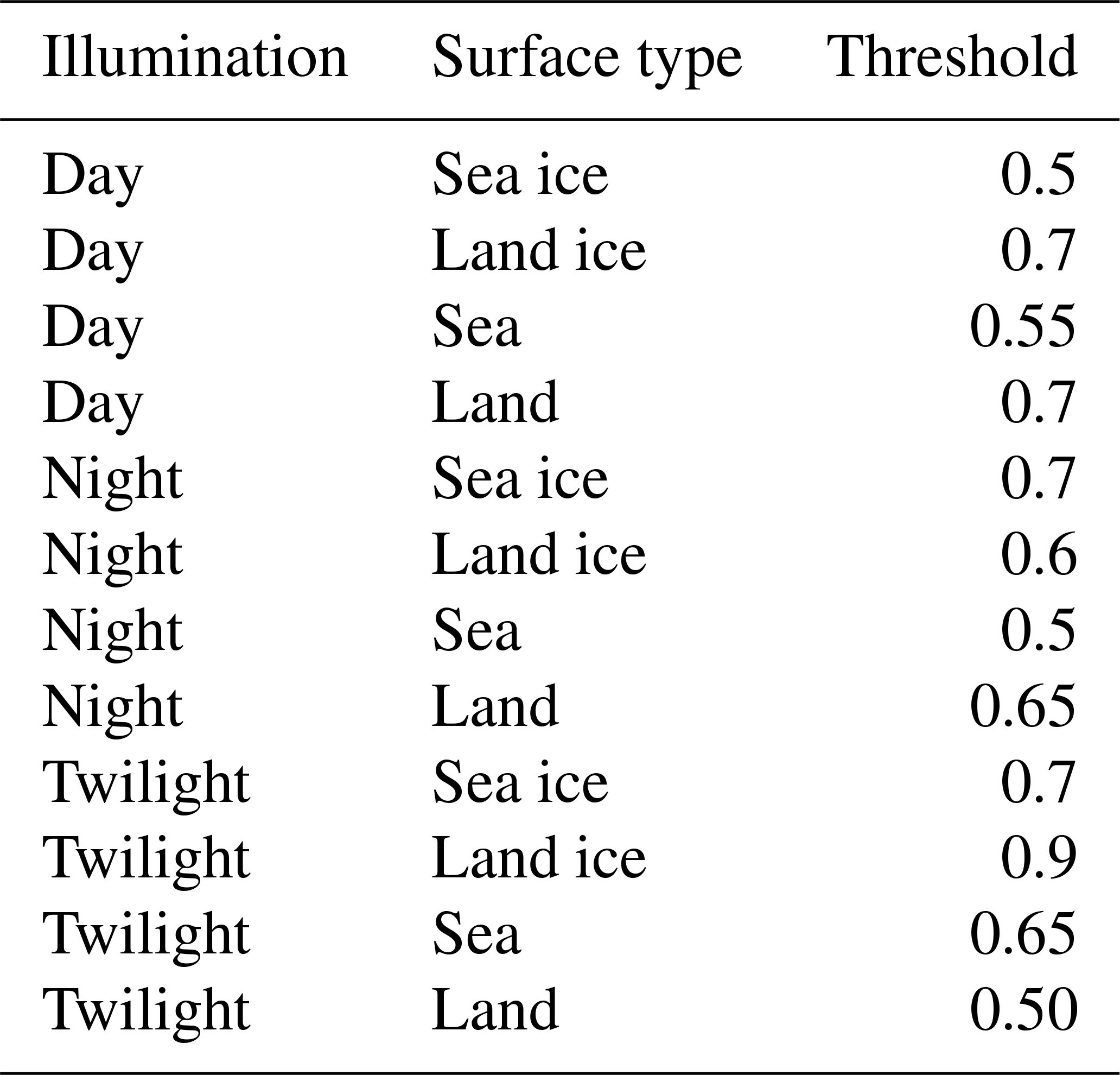
• Cloud mask (CMA). The ANN for cloud detection (ANN_mask) has been retrained using a much larger set of training data (approx. 10 times more collocation data used for v3 than for v2), which is composed of collocations between AVHRR measurements and cloud optical depth observed by the Cloud-Aerosol Lidar with Orthogonal Polarization (CALIOP; Winker et al., 2009). In addition, the 3.7 µm channel is now included for daytime conditions in the ANN scheme (exception: 1.6 µm is used for NOAA-16 for the period April 2001 to April 2003). Table B1 summarizes the ANN_mask input data as a function of illumination conditions, while Table B2 reports the empirical thresholds that are applied subsequently to convert the ANN_mask output into a binary cloud mask. Downstream, cloud detection is complemented by an additional cirrus test based on 10.8 and 12.0 µm IR measurements as defined in Pavolonis et al. (2005). As the cloud detection was developed and fine-tuned for AVHRR aboard the NOAA-19 satellite, SBAs are applied for other sensors, which are described in Appendix B. Cloud detection improvements compared to v2 are mainly found for daytime and twilight conditions in general but in particular also for conditions with snow or ice covered surfaces and in cases of low-level liquid clouds over the subtropical and tropical oceans. Validation scores are presented in Sect. 2.3, reflecting the improvements on the global scale.

• Cloud-top phase (CPH). The determination of the cloud-top phase, which in v2 was inferred from the cloud typing procedure of Pavolonis and Heidinger (2004) and Pavolonis et al. (2005), was replaced by an ANN approach for v3 (ANN_phase). The strategy for training the ANN_phase was very similar compared to the cloud detection approach: training the ANN_phase to emulate CALIOP cloud-top phase using AVHRR measurements as primary input data. The exact list of input data for the ANN_phase is given in Table B3. Table B4 lists the thresholds applied to convert the ANN_phase output into a binary cloud phase. As for cloud detection, SBAs are applied prior to the cloud phase determination (see Appendix B). Significant improvements are found for the cloud phase in v3 compared to v2 when analysing validation results against CALIOP as reported in Sect. 2.3.

• OE retrieval of cloud properties. The surface reflectance model was revised, leading to a corrected handling of the solar zenith angle (SZA), with the most pronounced changes at large angles. Furthermore, bugs were fixed in the code that composes the look-up tables (LUTs) based on pre-calculated radiative transfer simulations. In particular the LUTs for channels with solar-reflectance contribution changed considerably. This led to smaller cloud effective radius (CER) retrievals for 3.7 µm measurements, in particular for CER of ice clouds (CER_ice). Introducing the utilization of the ice cloud single-scattering properties of Baum et al. (2014) (Baran et al., 2005, used before) further reduced the CER_ice. For AVHRR-PMv3, cloud optical properties are also retrieved during night-time, facilitated by a differential sensitivity of the radiation in the spectral bands 3.7 and 10.8 µm (or 12.0 µm) to cloud optical thickness (COT) and CER. Night-time COT and CER retrievals are considered to be experimental products and only included in Level-3U products. All retrieved cloud properties are input to the calculation of the radiative fluxes as described in Sect. 3. As for v2, retrievals of COT and CER are used in v3 to determine liquid water path (LWP) and ice water path (IWP) following Stephens (1978).

2.2 Cloud property examples

Figure 1 shows global maps of monthly mean CFC, liquid cloud fraction (LCF), COT and CER for June 2014 for v3 Level-3C data – along with the same data from v2. In general, global patterns look very similar, with only minor differences between v3 and v2 for CFC and COT. LCF increased (more liquid clouds) from v3 to v2 after a fundamental change of the phase detection approach (see above). CER of v3 is significantly lower than in v2, which is mainly due to fixing a bug in some CC4CL LUTs and introducing alternative single-scattering properties, as mentioned in Sect. 2.1, which only affected retrieved ice cloud properties.

Figure 2 presents the same comparison for cloud-top pressure (CTP), LWP, IWP and cloud albedo at 0.6 µm (CLA_0.6). Global patterns remain very similar again. Mean CTP is higher in v3 than in v2 in the tropics, which is predominantly due to detecting more very low-level clouds above tropical oceans. While LWP remains similar in v3 compared to v2, IWP is significantly lower in v3 due to lower CER_ice (input to the IWP calculation). Unrealistically high LWP and IWP values in polar regions are reduced in v3 due to reduced CER. CLA_0.6 is slightly higher in v3 compared to v2, although the changes are relatively small.

Detailed validation was carried out for all cloud properties for which accurate reference data exist. The results of those efforts are presented in the next section, highlighting the quality of the v3 data.

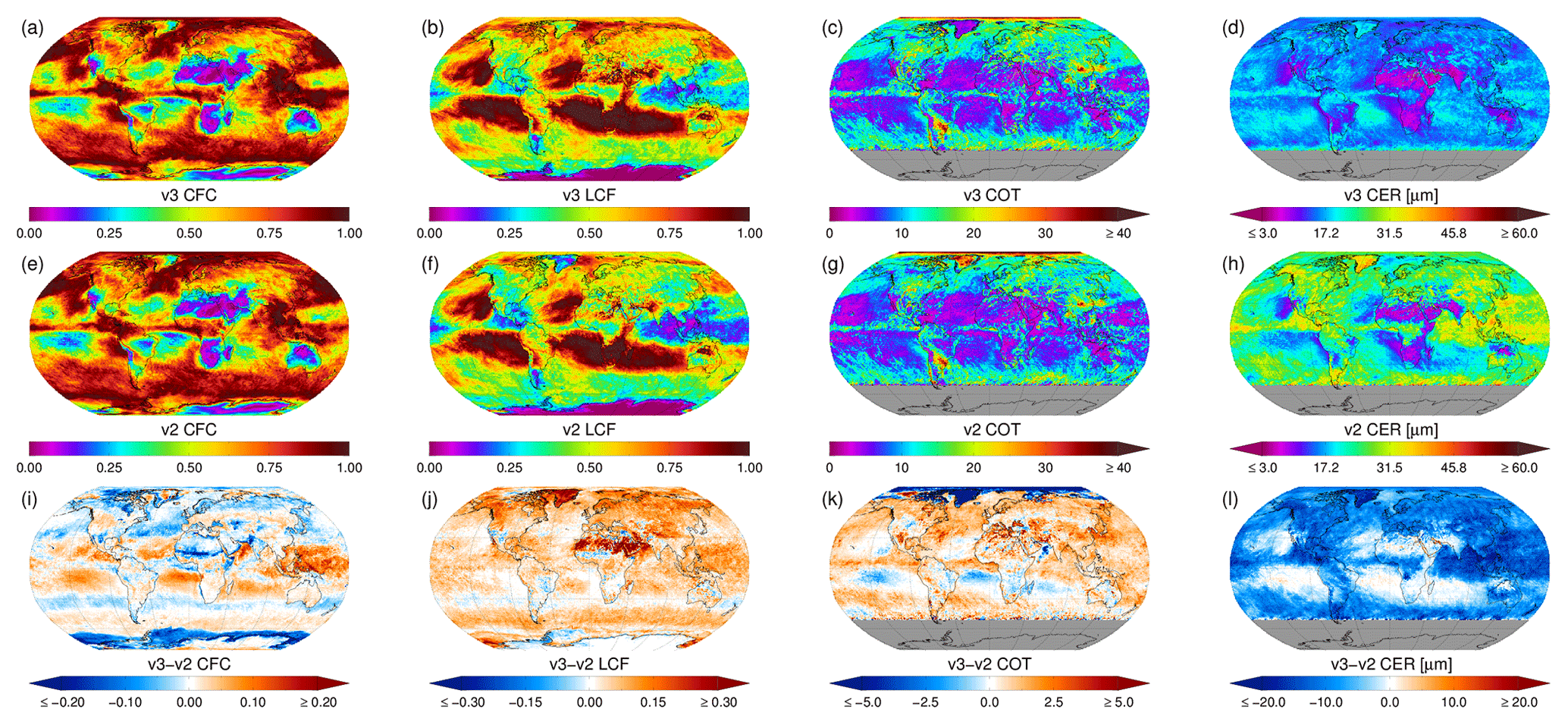
Figure 1 Examples of Level-3C (monthly means) Cloud_cci AVHRR-PMv3 data for cloud fraction (CFC) (a), liquid cloud fraction (LCF) (b), cloud optical thickness (COT) (c) and cloud effective radius (CER) (d). Same data are shown for v2 (e)–(h). Difference maps are shown in panels (i)–(l). All data are from June 2014.

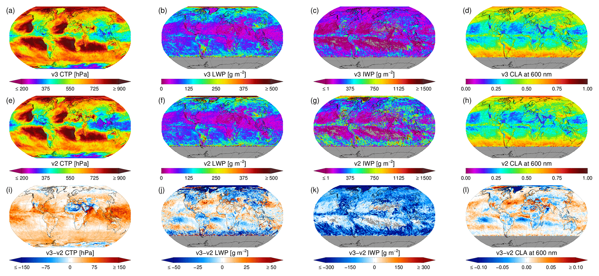
Figure 2 As in Fig. 1 but for CTP, LWP, IWP and CLA.

2.3 Validation

Cloud_cci AVHRR-PMv3 CMA, CPH and cloud-top height (CTH) Level-3U products were collocated with equivalent CALIOP products which are assumed to be of superior quality. More specifically, the CAL_LID_L2_05kmCLay-Prov product was downloaded from the ICARE Data and Service Center (http://www.icare.univ-lille1.fr, last access: 29 March 2017). The collocations between CALIOP and the AVHRR-PM data were done as reported in Stengel et al. (2017), with the most important fact being that only those collocations were included for which the spatial and temporal mismatch was below 5 km and 3 min, respectively. These criteria were chosen as a compromise between using the best spatial and temporal matches and allowing for compositions of a sound database to be used in the validation. It is important to note that the random deviations of AVHRR-PM to CALIOP depend on the defined criteria, while the systematic ones most likely do not. To investigate the sensitivity of passive imager retrievals to the thinnest cloud layers, the cloud optical depth profiles included in the CALIOP profiles were employed as in Karlsson and Johansson (2013), Stengel et al. (2013), and Sus et al. (2018). Following this approach different scenarios for excluding optically thin cloud layers are investigated when discussing validation of CMA, CPH and CTH below.

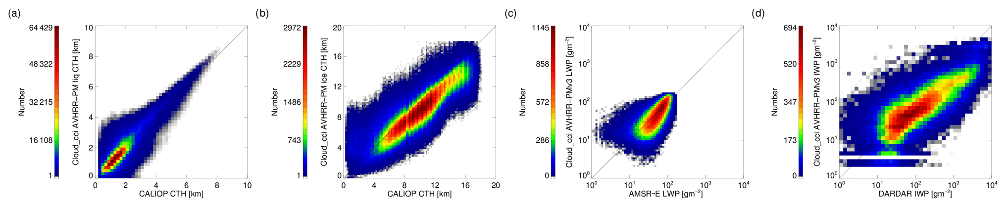
Figure 3 Two-dimensional frequency distributions of AVHRR-PMv3 cloud properties (a: cloud-top height – CTH – of liquid clouds; b: cloud-top height of ice clouds; c: liquid water path – LWP; d: ice water path – IWP) collocated with corresponding reference products of CALIOP, AMSR-E and DARDAR.

In addition to the validation against CALIOP, Cloud_cci AVHRR-PMv3 LWP was collocated with the Advanced Microwave Scanning Radiometer – Earth Observing System (AMSR-E) observations of LWP (Wentz and Meissner, 2004), and IWP was collocated to DARDAR (raDAR–liDAR; Delanoë and Hogan, 2008, 2010) observations of IWP. Passive microwave observations of AMSR-E over ocean and active observations of CALIOP and CloudSat in DARDAR are assumed to provide the best reference data for LWP and IWP on global scales. All validation results are accompanied by the equivalent results for v2.

Table 2 reports the validation results for CMA for two scenarios: (1) considering all CALIOP reference pixels for which the CALIOP COT is above 0.0 (COT_thres=0.0) to be cloudy and (2) considering only those CALIOP reference pixels for which the CALIOP COT is above 0.15 (COT_thres=0.15) to be cloudy. The latter scenario is added to account for the lack of sensitivity of AVHRR measurements to very optically thin clouds. For both scenarios, the scores are generally better for v3 than for v2. Heidke skill scores (HSSs; Heidke, 1926), hit rates and probabilities of detections (PODs) are higher (thus better). The only degradation in the scores is found for the bias, which is slightly more negative in v3 compared to v2.

Table 3 reports the validation results for CPH for two scenarios: (1) using the cloud phase at the top of the uppermost cloud layer detected by CALIOP as a reference (COT_lev=0.0) and (2) using the cloud phase at an optical depth of 0.15 into the cloud (top-down) as a reference (COT_lev=0.15). Comparing the HSS as an overall measure for the correct cloud phase detection, v3 performs better than v2. The POD of liquid clouds is significantly improved in v3, while a small degradation in POD of ice clouds is found in v3 compared to v2. The liquid bias increased for v3. Removing the thinnest cloud layers, thus accounting for the AVHRR sensor limitation, the improvement of v3 over v2 becomes even clearer. In this scenario, the cloud phase of 84.7 % of all clouds is correctly identified in v3 (according to hit rate scores). It is important to note that the CALIOP data used for validation of cloud detection and cloud phase determination excluded the data that were used for training the ANNs.

Table 4 reports the validation results for CTH. The validation is stratified by the phase of the cloud and by the optical depth into the cloud (top-down) at which the reference CTH is taken from the CALIOP profile. In addition to COT_lev of 0.0 and 0.15, a COT_lev of 1.0 is also included. Generally only few changes in validation scores are found between v3 and v2. While for liquid clouds the scores remain nearly the same, a small degradation in the CTH bias for ice clouds is found. The underestimation of CTH is stronger in v3 compared to v2. For example for the geometrical CTH from CALIOP (COT_lev=0.0), the bias degrades, from −2.594 to −3.54 km. One reason for this can be that the LUT-related bug fixes (see Sect. 2.1) led to smaller CER_ice values. Smaller ice particles absorb less radiation coming from below the cloud, putting the cloud lower in the atmosphere in the retrieval. In contrast to the bias, standard deviations are reduced for v3, amounting to 2.36 km compared to 2.51 km in v2. For COT_lev=0.15 and COT_lev=1.0, very similar findings are seen, with both of these scenarios showing the reduction in bias and standard deviation with an increasing COT_lev for ice clouds. This highlights the difficulties in correctly placing (vertically) optically thin clouds and cloud layers when using AVHRR measurements. Figure 3 shows two-dimensional frequency distributions of all data included in the CTH validation statistics for COT_lev=1.0 (Fig. 3a for liquid clouds and Fig. 3b for ice clouds).

Table 5 reports the validation results for LWP. Although the bias for v3 remains small when compared with AMSR-E, it is slightly increased compared to v2, from −1.9 to −3.2 g m⁻². Standard deviations are slightly decreased for v3 (26.4 g m⁻²) compared to v2 (27.1 g m⁻²), and the correlation remains unchanged at 0.64. Figure 3c shows the two-dimensional frequency distribution of all data included in the LWP validation statistics.

Table 6 reports the validation results for IWP. The AVHRR-PM IWP generally shows an underestimation of IWP when DARDAR is considered to be a reference. This underestimation has increased for v3 as the bias has become larger and negative (−307.1 g m⁻² for v3 compared to 33.3 g m⁻² for v2). However, the standard deviation has decreased significantly, from 1299.8 to 900.9 g m⁻², along with a clear increase in correlation, from 0.42 to 0.63. Figure 3d shows the two-dimensional frequency distribution of all data included in the IWP validation statistics.

Despite the assumption that the reference data used are of higher quality than the Cloud_cci data, uncertainties and inaccuracies remain in the reference data as well, which should be kept in mind when interpreting the presented validation scores. However, summarizing the discussion above, the cloud properties included in AVHRR-PMv3 are considered to be of more superior quality than the precursor version.

An even broader assessment of the quality of the presented dataset can be found in PVIR (2019), in which the results are also stratified by illumination conditions along with other conditions.

Table 2 Cloud mask (CMA) validation results for Cloud_cci AVHRR-PMv3 when compared with CALIOP. Validation results for AVHRR-PMv2 are also reported. Validation measures are Heidke skill score (HSS), hit rate, the probabilities of detecting cloudy and clear scenes (POD_cloudy and POD_clear), and bias. In addition, the number of collocated pixels is given. The scores are separated into two cloud optical thickness thresholds (COT_thres) reflecting the CALIOP COT above which the CALIOP pixel was classified cloudy.

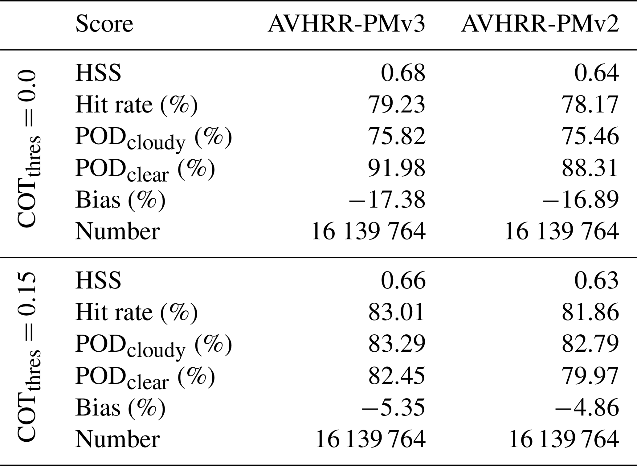
Table 3 Cloud phase (CPH) validation results for Cloud_cci AVHRR-PMv3 when compared with CALIOP. Validation results for AVHRR-PMv2 are also reported. Validation measures are Heidke skill score (HSS), hit rate, the probabilities of detecting liquid and ice phase (POD_liq, POD_ice), and bias of liquid cloud occurrence. In addition the number of collocated pixels is given. The scores are separated into two cloud optical depth levels (COT_lev) representing the top-down COT into the cloud at which the reference CALIOP CPH was taken.

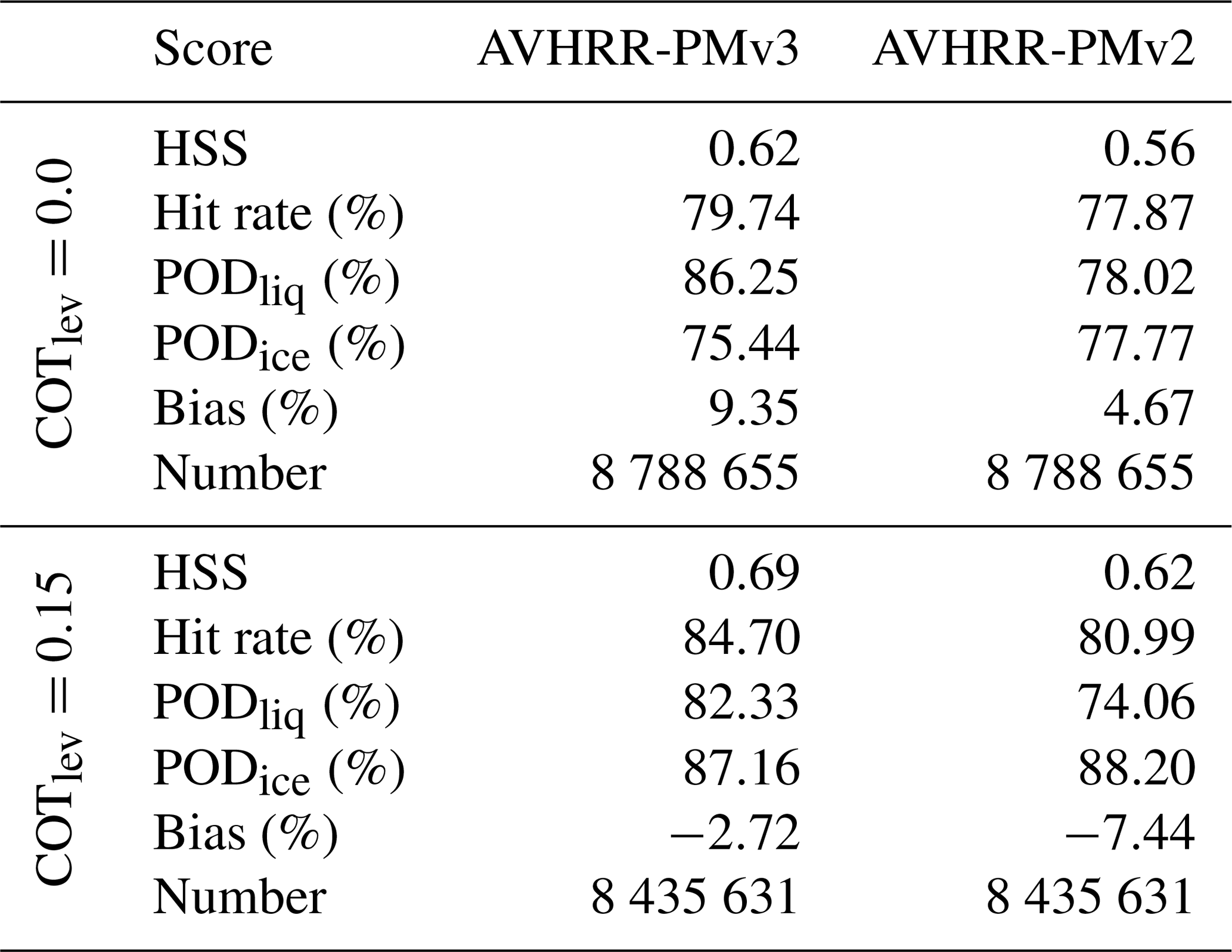
Table 4 Cloud-top height (CTH) validation results for Cloud_cci AVHRR-PMv3 when compared with CALIOP. Validation results for AVHRR-PMv2 are also reported. Validation measures are standard deviation (SD) of the error and the mean error (bias). In addition the number of collocated pixels is given. All scores are separated into liquid and ice clouds (both Cloud_cci dataset and CALIOP had to agree on phase) and into three cloud optical depth levels (COT_lev) representing the top-down COT into the cloud at which the reference CALIOP CTH was taken.

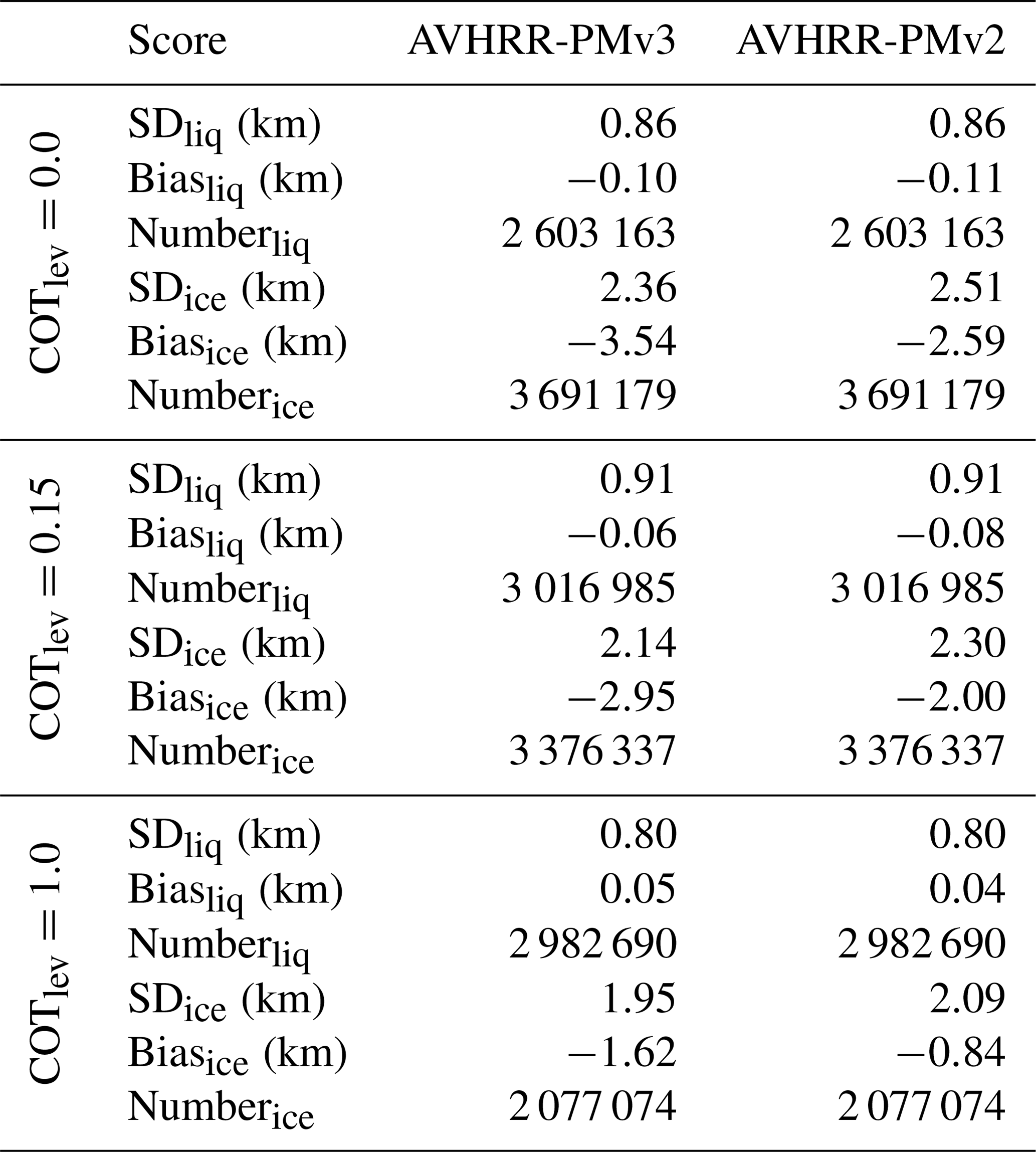
Table 5 Liquid water path (LWP) validation results for Cloud_cci AVHRR-PMv3 when compared with AMSR-E for the year 2008. Validation results for AVHRR-PMv2 for the same time period are also reported. Validation measures are standard deviation (SD) of the error, the mean error (bias) and correlation. In addition the number of collocated pixels is given.

Table 6 Ice water path (IWP) validation results for Cloud_cci AVHRR-PMv3 when compared with DARDAR for January to July 2008. Validation results for AVHRR-PMv2 for the same time period are also reported. Validation measures are standard deviation (SD) of the error, the mean error (bias) and correlation. In addition the number of collocated pixels is given.

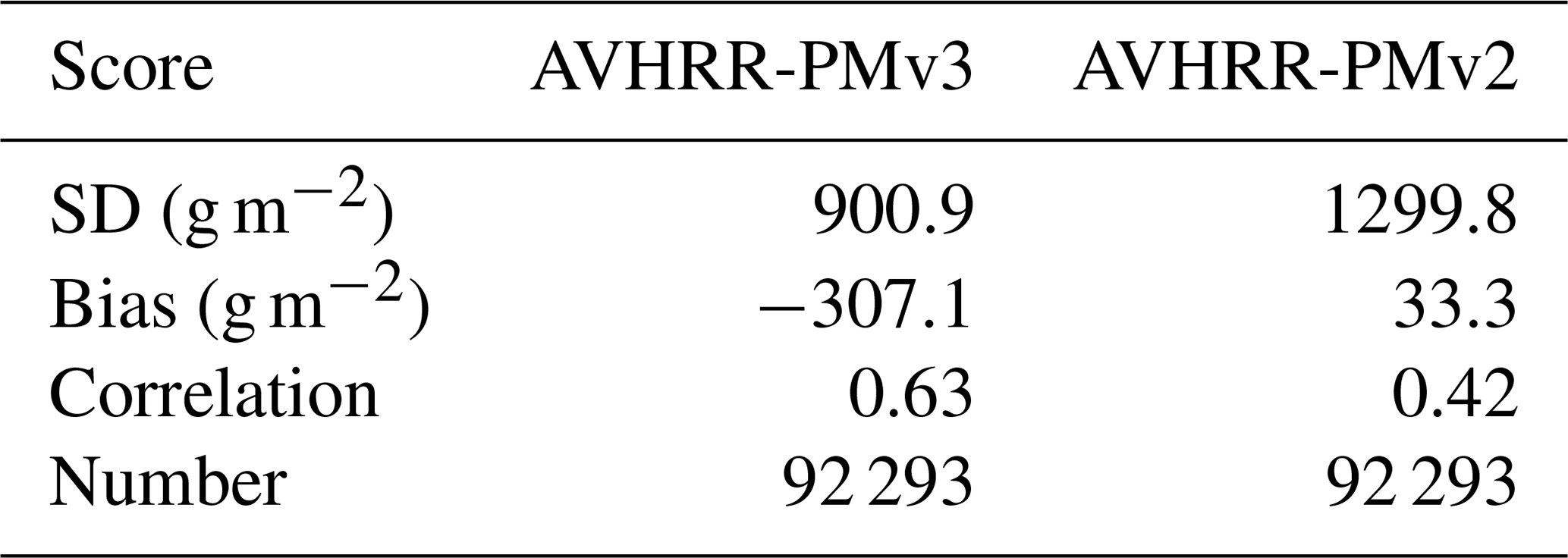
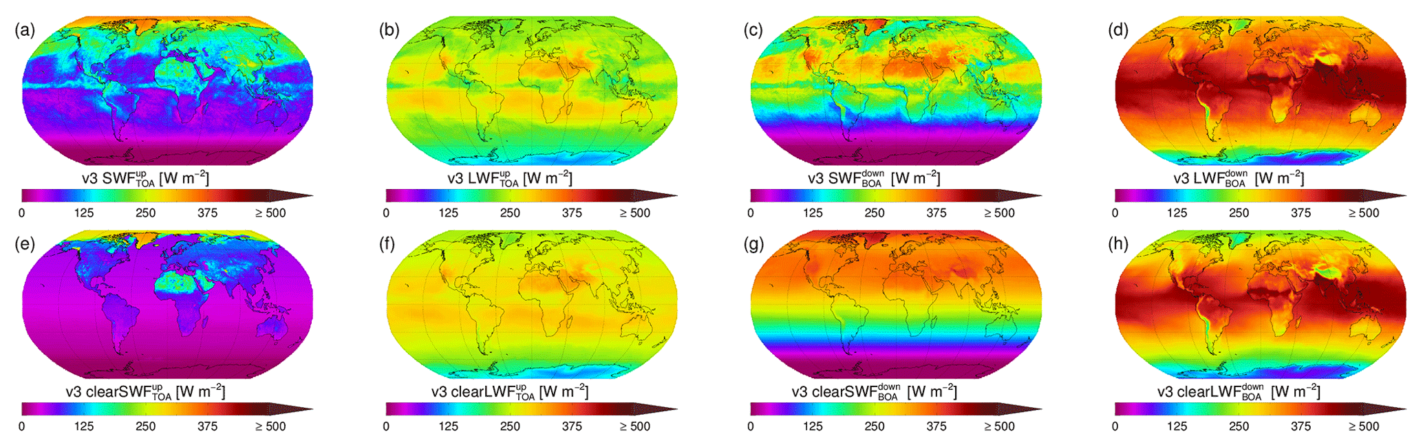
Figure 4 Examples of Level-3C (monthly means) Cloud_cci AVHRR-PMv3 data of ${\text{SWF}}_{\text{TOA}}^{\text{up}}$, ${\text{LWF}}_{\text{TOA}}^{\text{up}}$, ${\text{SWF}}_{\text{BOA}}^{\text{down}}$ and ${\text{LWF}}_{\text{BOA}}^{\text{down}}$ (a–d). ${\text{clearSWF}}_{\text{TOA}}^{\text{up}}$, ${\text{clearLWF}}_{\text{TOA}}^{\text{up}}$, ${\text{clearSWF}}_{\text{BOA}}^{\text{down}}$ and ${\text{clearLWF}}_{\text{BOA}}^{\text{down}}$ are shown in (e)–(h), representing the same fluxes as in (a)–(d) but for clear-sky conditions. All data are from June 2014.

Table 7 Validation results for monthly Cloud_cci AVHRR-PMv3 shortwave and longwave and downwelling and upwelling radiative fluxes at bottom of atmosphere (BOA) when compared with Baseline Surface Radiation Network (BSRN) sites within the period 2003–2016. Validation measures are standard deviation (SD), bias and correlation. In addition the number of data pairs is given.

3 Radiation properties

In addition to the cloud properties described in the previous section, radiative broadband flux properties (shortwave and longwave) at the TOA and BOA, and for all-sky and clear-sky conditions, were calculated employing the BUGSrad scheme (Stephens et al., 2001, more details below). Furthermore, the photosynthetic active radiation was determined, which is the BOA downwelling shortwave radiation in the spectral range between 400 and 700 nm. A full list of radiation properties is given in the bottom part of Table 1. As for the cloud properties, all radiation properties are derived at pixel level, subsampled to daily and global composites (Level-3U products) and aggregated to monthly Level-3C products.

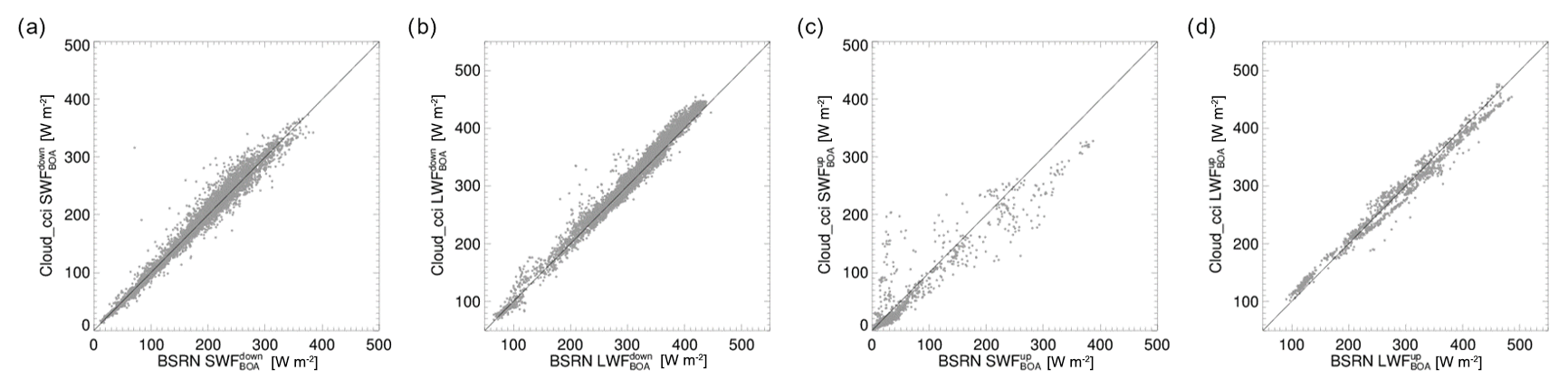
Figure 5 Comparison of Cloud_cci bottom of atmosphere (BOA) shortwave (SW; panel a) and longwave (LW; panel b) downwelling fluxes with ground-based reference measurements taken at globally distributed Baseline Surface Radiation Network (BSRN) sites for which equivalent reference data were available. Panels (c) and (d) are as in (a) and (b) but for upwelling fluxes. Shown are all monthly data pairs within the period 2003–2016.

Figure 6 Multi-annual (2003–2016) mean downwelling shortwave (SW) radiative fluxes at bottom of atmosphere (BOA) for all-sky conditions for Cloud_cci AVHRR-PMv3 (a) and CERES EBAF surface fluxes (b). Panels (d) and (e) show the same data but for clear-sky conditions. Panels (c) and (f) show difference plots Cloud_cci minus CERES.

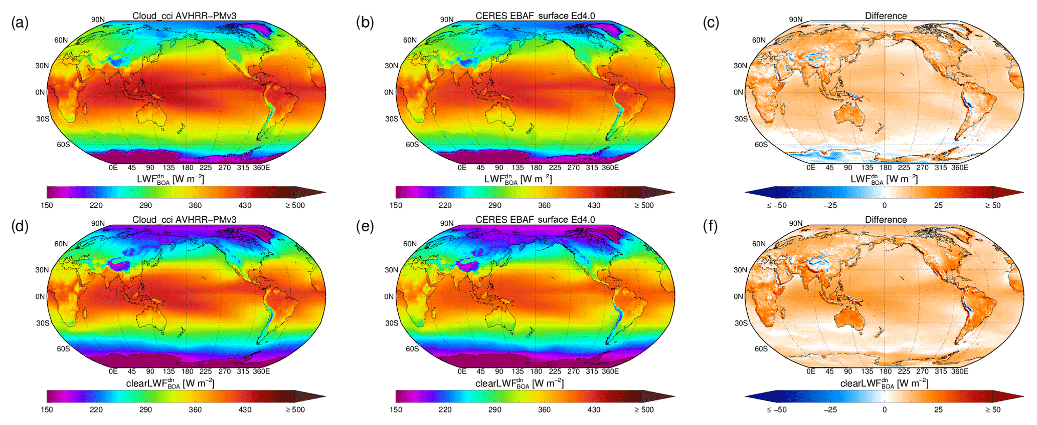
Figure 7 Multi-annual (2003–2016) mean downwelling longwave (LW) radiative fluxes at bottom of atmosphere (BOA) for all-sky conditions for Cloud_cci AVHRR-PMv3 (a) and CERES EBAF surface fluxes (b). Panels (d) and (e) show the same data but for clear-sky conditions. Panels (c) and (f) show difference plots Cloud_cci minus CERES.

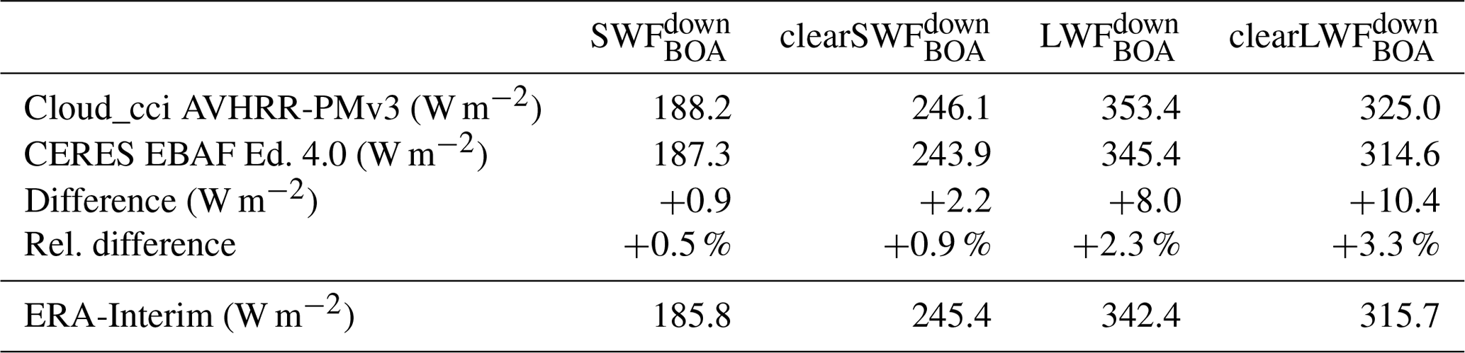
Table 8 Multi-annual (2003–2016), latitude-weighted, global mean downwelling broadband shortwave fluxes and longwave fluxes (SWFs and LWFs) at bottom of atmosphere (BOA) inferred from Cloud_cci AVHRR-PMv3 dataset for all-sky and clear-sky (clear) conditions. The values are compared to equivalents inferred from Clouds and the Earth's Radiant Energy System (CERES) Energy Balanced and Filled (EBAF) surface fluxes. All values are given in watts per square metre (W m⁻²). In addition, differences and relative differences (Cloud_cci-CERES) for all fluxes are reported. For comparison, ERA-Interim values are listed as well.

Table 9 As Table 8 but for BOA upwelling broadband fluxes.

3.1 Algorithm

BUGSrad uses a two-stream approximation along with correlated-k distribution methods for atmospheric radiative transfer (Fu and Liou, 1992). It has been used to investigate aerosol–cloud interactions (Christensen et al., 2017) and to assess the Earth's energy budget using CloudSat observations (Stephens et al., 2012). BUGSrad is applied to a single-column, plane-parallel atmosphere with ingested cloud properties (i.e. CER, COT and CTP) previously retrieved with CC4CL (see Sect. 2.1). BUGSrad uses 18 spectral bands in the electromagnetic spectrum (6 in the shortwave and 12 in the longwave spectrum) to compute the broadband fluxes. Atmospheric profiles for temperature and water vapour are taken from ERA-Interim. Visible and near-infrared surface albedo are based on spatio-temporally resolved MODIS climatologies – with all data being identical to the usage in CC4CL. Total solar irradiance is based on SOHO (Solar and Heliospheric Observatory) and SORCE (SOlar Radiation and Climate Experiment) measurements acquired from http://disc.sci.gsfc.nasa.gov/SORCE/data-holdingsusingSOR3TSID_v017 (last access: 12 December 2019) and further processed by applying a bilinear interpolation followed by a bias correction to SOHO measurements to match SORCE. For well-mixed radiatively important trace gases, constant values are used (CH₄ =1.8 ppm; N₂O =0.26 ppm). For CO₂ a linearly time-dependent concentration is used, anchored at 380 ppm for the year 2006. To account for the effect of aerosols on the radiation, an aerosol optical depth of 0.05 was added to the extinction throughout the atmosphere. It is acknowledged that this value under-represents heavy aerosol loadings, which motivates the utilization of spatio-temporally resolved aerosol information for future dataset versions. The reader is referred to ATBD-CC4CL-BBFlux (2019) for more details on the calculation of the broadband fluxes.

Due to the angular dependence of the solar illumination together with the low sampling frequency of a single polar-orbiting AVHRR sensor, an angular-dependent correction is applied to the shortwave radiation properties to make the data represent 24 h averages. This is done by calculating the diurnal cycle of the SZA for a given pixel on the day of observation. The diurnal cycle of SZA is then used to rescale the incoming and reflected solar radiation and adjust the surface albedo (using an empirical quadratic function of SZA) and the atmospheric path length for a given set of time stamps throughout the local day. Averaging these samples gives a suitable approximation for a true 24 h mean, which is needed to determine true climatological means. This procedure is, however, only applied for Level-3C products, while Level-3U products hold the instantaneous, uncorrected fluxes representing the solar illumination at the pixel location and at the time of observation.

For longwave radiation, a diurnal cycle correction is applied over land based on a cosine fit to an observed mean diurnal cycle by applying CC4CL to the geostationary Spinning Enhanced Visible and Infrared Imager (SEVIRI). The observed diurnal cycle is converted into a correction factor, which itself is a function of local observation time, to mimic a 24 h mean.

In contrast to the cloud properties, the radiative fluxes in the presented dataset version are not accompanied by uncertainty estimates on pixel level. While the validation results presented below provide general guidance for the quality of the radiative fluxes, users of the data are also encouraged to inspect the pixel-level uncertainties of the cloud properties, as these are dominant input to the calculation of the fluxes.

3.2 Radiation property examples

Figure 4 shows examples of Cloud_cci AVHRR-PMv3 Level-3C data of ${\text{SWF}}_{\text{TOA}}^{\text{up}}$, ${\text{LWF}}_{\text{TOA}}^{\text{up}}$, ${\text{SWF}}_{\text{BOA}}^{\text{down}}$ and ${\text{LWF}}_{\text{BOA}}^{\text{down}}$ for all-sky and clear-sky conditions for June 2014. As a general description of these properties, high ${\text{clearSWF}}_{\text{TOA}}^{\text{up}}$ is found in regions with high surface albedo, while high values in ${\text{SWF}}_{\text{TOA}}^{\text{up}}$ are additionally visible in regions with a high cloud fraction and vice versa. ${\text{clearSWF}}_{\text{TOA}}^{\text{up}}$ and ${\text{SWF}}_{\text{TOA}}^{\text{up}}$ depend on incoming solar flux, which, in the month of June, is highest in the tropics and Northern Hemisphere. ${\text{clearLWF}}_{\text{TOA}}^{\text{up}}$ is highest in regions with high surface temperatures and low water vapour amounts in the atmospheric column above. Higher water vapour loadings and in particular frequent occurrence of cold clouds significantly reduce the ${\text{LWF}}_{\text{TOA}}^{\text{up}}$; this is, for example, visible in the tropics and the mid-latitudes. ${\text{SWF}}_{\text{BOA}}^{\text{down}}$ represents the downwelling solar radiation that is neither reflected nor absorbed by clouds or the atmosphere and is thus, roughly speaking, high where ${\text{SWF}}_{\text{TOA}}^{\text{up}}$ is low and vice versa. ${\text{SWF}}_{\text{BOA}}^{\text{down}}$ and ${\text{clearSWF}}_{\text{BOA}}^{\text{down}}$ strongly depend on illumination conditions. ${\text{LWF}}_{\text{BOA}}^{\text{down}}$ represents the downwelling radiation emitted by the atmosphere and clouds and is high in regions with high water vapour amounts and further increased when clouds are frequently present.

The product portfolio for radiative fluxes is complemented by ${\text{SWF}}_{\text{TOA}}^{\text{down}}$, the incoming solar radiation at the top of the atmosphere, ${\text{SWF}}_{\text{BOA}}^{\text{up}}$ (${\text{LWF}}_{\text{BOA}}^{\text{up}}$), the reflected solar (emitted terrestrial) radiation at the Earth's surface (not shown), and PAR.

3.3 Validation

3.3.1 BOA radiative fluxes

The Cloud_cci AVHRR-PMv3 BOA radiative fluxes ${\text{SWF}}_{\text{BOA}}^{\text{down}}$ and ${\text{LWF}}_{\text{BOA}}^{\text{down}}$ were compared with ground-based reference stations of the World Radiation Monitoring Center (WRMC) Baseline Surface Radiation Network (BSRN; Driemel et al., 2018). For this, monthly mean BSRN ${\text{SWF}}_{\text{BOA}}^{\text{down}}$ and ${\text{LWF}}_{\text{BOA}}^{\text{down}}$ values were calculated per station from all available observations and then compared to the nearest-neighbouring Cloud_cci grid box. Figure 5 shows scatter plots for all monthly pairs found within the period of 2003 to 2016. The validation scores are reported in Table 7. An excellent agreement of the Cloud_cci with the reference BSRN measurements is found for both ${\text{SWF}}_{\text{BOA}}^{\text{down}}$ and ${\text{LWF}}_{\text{BOA}}^{\text{down}}$ products, with correlations above 0.98. Standard deviations are 13.8 W m⁻² for ${\text{SWF}}_{\text{BOA}}^{\text{down}}$ and 11.5 W m⁻² for ${\text{LWF}}_{\text{BOA}}^{\text{down}}$. The comparisons further reveal positive biases in Cloud_cci: 1.9 W m⁻² for ${\text{SWF}}_{\text{BOA}}^{\text{down}}$ and 7.6 W m⁻² for ${\text{LWF}}_{\text{BOA}}^{\text{down}}$. Considering the ${\text{LWF}}_{\text{BOA}}^{\text{down}}$ bias, Nyeki et al. (2017) recently found indications that the measured fluxes at BSRN stations are biased low. They quantified this with 3.5 to 5.4 W m⁻², which has the potential to explain more than 50 % of the bias found between Cloud_cci and BSRN for ${\text{LWF}}_{\text{BOA}}^{\text{down}}$. Figure 5 also shows equivalent validation for upwelling fluxes at those BSRN sites which provide upwelling measurements (much fewer stations than for downwelling fluxes). For ${\text{LWF}}_{\text{BOA}}^{\text{up}}$ the agreement of Cloud_cci to BSRN is again very good, with a standard deviation of 14.1 W m⁻², a bias of −3.0 W m⁻² and a correlation of 0.99.

In general, the agreement of the Cloud_cci ${\text{SWF}}_{\text{BOA}}^{\text{down}}$, ${\text{LWF}}_{\text{BOA}}^{\text{down}}$ and ${\text{LWF}}_{\text{BOA}}^{\text{up}}$ with the BSRN stations is remarkable when considering that only one satellite sensor is used at a time; thus for many locations on Earth only two satellite overpasses (one daytime and one night-time) within 24 h provide observations. The results are a confirmation that the developed and applied diurnal cycle correction works well, which is more important for the shortwave than for the longwave fluxes.

In contrast, for ${\text{SWF}}_{\text{BOA}}^{\text{up}}$ more scatter is found in the comparisons to BSRN. Considering that ${\text{SWF}}_{\text{BOA}}^{\text{up}}$ is simply the ${\text{SWF}}_{\text{BOA}}^{\text{down}}$ multiplied by the surface albedo, and the good validation results for ${\text{SWF}}_{\text{BOA}}^{\text{down}}$, this leads to the conclusions that either imperfect surface albedo was used in Cloud_cci or, more likely, the difference in spatial scales might be the dominating source of the discrepancy found. Fine-scale inhomogeneities in surface albedo in the vicinity of the BSRN stations will propagate into the results.

In addition to the BSRN stations, Cloud_cci BOA downwelling and upwelling fluxes were compared to the Clouds and the Earth's Radiant Energy System (CERES) Energy Balanced and Filled (EBAF) surface flux product (Kato et al., 2013), i.e. by means of comparing multi-annual mean maps for the period 2003–2016 (Figs. 6 and 7), with corresponding latitude-weighted global mean values given in Table 8.

The Cloud_cci multi-annual mean maps of ${\text{SWF}}_{\text{BOA}}^{\text{down}}$ for the chosen period agree very well with the CERES products (Fig. 6a and b) and for the clear-sky fluxes (Fig. 6d and e). This is also supported by global mean values reported in Table 8, in which Cloud_cci is slightly biased high (+0.9 W m⁻² for ${\text{SWF}}_{\text{BOA}}^{\text{down}}$ and +2.2 W m⁻² for ${\text{clearSWF}}_{\text{BOA}}^{\text{down}}$). Clear-sky fluxes in both products are mainly characterized by larger incoming solar radiation at the Equator, scattering and absorption by atmospheric gases and aerosols, and the surface reflectivity and emissivity. The presence of clouds usually leads to a significant reduction of ${\text{SWF}}_{\text{BOA}}^{\text{down}}$ locally, being a function of optical thickness and cloud fraction over larger domains. The fact that the all-sky fluxes ${\text{SWF}}_{\text{BOA}}^{\text{down}}$ agree very well with CERES validates the Cloud_cci cloud detection and corresponding cloud property retrievals, which can thus be assumed to be of high quality.

The Cloud_cci multi-annual mean maps of ${\text{LWF}}_{\text{BOA}}^{\text{down}}$ (Fig. 7) also agree well with CERES in terms of global patterns. The absolute values, however, show systematically higher values for Cloud_cci of about 8 to 9 W m⁻² for both all-sky and clear-sky values. The positive bias is relatively homogenous over the globe. In relative terms the systematic differences amount to approximately 2 % to 3 %. However, these differences lie within the expected range of the CERES accuracy (Rutan et al., 2015).

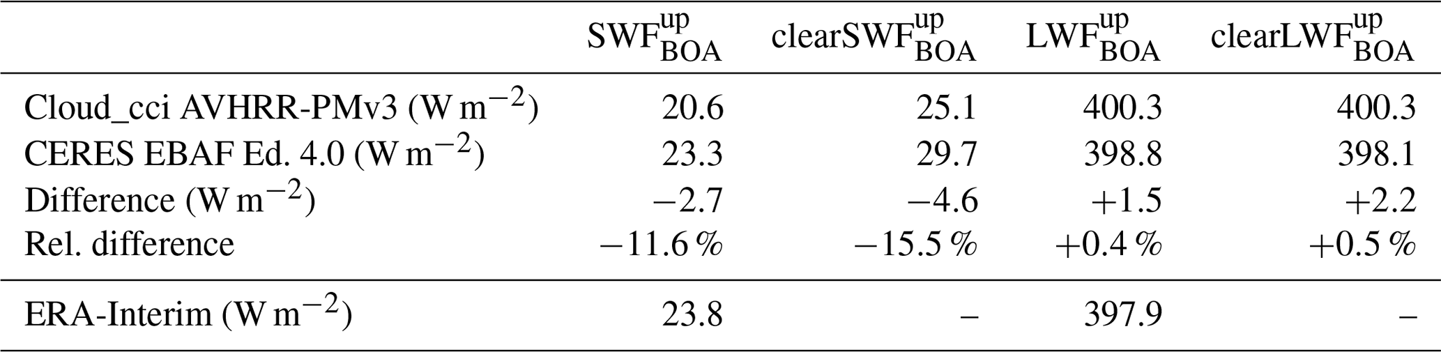
The Cloud_cci multi-annual mean maps of ${\text{SWF}}_{\text{BOA}}^{\text{up}}$ exhibit larger systematic deviations (not shown) than for ${\text{SWF}}_{\text{BOA}}^{\text{down}}$. The larger standard deviations retrieved for the solar reflected radiation are primarily related to variances in surface albedo which tend to have significant annual cycles. Global mean values reported in Table 9 give negative biases of −2.7 and −4.6 W m⁻² for Cloud_cci which in relative terms correspond to negative deviations of more than 10 %. It remains uncertain which of the two products are more realistic, as no real ground truth is available for ${\text{SWF}}_{\text{BOA}}^{\text{up}}$ that represents spatial scales of satellite pixels (several kilometres). Repeating the validation of ${\text{SWF}}_{\text{BOA}}^{\text{up}}$ against BSRN but using CERES gives comparable, large deviations (not shown), as found for Cloud_cci (see above). This is in agreement with the findings of (Kratz et al., 2010), who reported systematic deviations between CERES and surface observations of ${\text{SWF}}_{\text{BOA}}^{\text{up}}$ depending on the time of day, meteorological condition and location.

Cloud_cci multi-annual maps of ${\text{LWF}}_{\text{BOA}}^{\text{up}}$ are again closer to CERES (not shown). Global mean values (Table 9) deviate by approximately 2 W m⁻², with larger values only for Cloud_cci. In relative terms the differences are about 0.5 %.

3.3.2 TOA radiative fluxes

The Cloud_cci TOA radiative fluxes ${\text{SWF}}_{\text{TOA}}^{\text{up}}$ and ${\text{LWF}}_{\text{TOA}}^{\text{up}}$ were compared with the CERES EBAF TOA Edition 4.0 data (Loeb et al., 2018). As for the BOA fluxes the comparison includes multi-annual mean maps for the period 2003–2016. Figure 8 shows the maps for SWF for all-sky and clear-sky (${\text{clearSWF}}_{\text{TOA}}^{\text{up}}$) conditions. Cloud_cci global patterns are very similar to those of the CERES products. High ${\text{SWF}}_{\text{TOA}}^{\text{up}}$ values are found in regions with high surface albedo, e.g. deserts and polar regions, or with high cloud frequency, e.g. in mid-latitude storm track regions in both hemispheres, in the Intertropical Convergence Zone and in regions with persistent marine stratocumulus clouds. Most prominent regions with low ${\text{SWF}}_{\text{TOA}}^{\text{up}}$ values are the subtropical subsidence regions (low cloud frequency) over the ocean (low surface albedo). It can also be seen that Cloud_cci provides slightly higher values in regions with high SWF (mainly land). The comparisons of the clear-sky fluxes give very similar results, with the exception that Cloud_cci has generally slightly lower values than CERES over ocean. The global mean values given in Table 10 reveal differences of 2.9 and −3.3 W m⁻² for all-sky and clear-sky fluxes, respectively. The smaller values in Cloud_cci clear-sky are partly explained by the differences already found for ${\text{SWF}}_{\text{BOA}}^{\text{up}}$ (see previous section).

Figure 9 shows the results of an equivalent analysis for upwelling LWF at the TOA. The global Cloud_cci patterns are again in very good agreement with CERES. High ${\text{LWF}}_{\text{TOA}}^{\text{up}}$ values are mainly found in tropical and subtropical regions (high surface temperature) with low cloud frequency or in regions with mainly low-level clouds (marine stratocumulus or trade cumulus regions), where the cloud-top temperatures are relatively warm. On the contrary, ${\text{LWF}}_{\text{TOA}}^{\text{up}}$ is low in regions with cold surfaces (e.g. polar regions) and regions with a high frequency of cold clouds. Cloud_cci ${\text{clearLWF}}_{\text{TOA}}^{\text{up}}$ values are dominated by surface temperatures, thus decreasing towards higher latitudes, generally showing a very good agreement with CERES. The difference maps, however, reveal that Cloud_cci has generally lower values than CERES for both all-sky and clear-sky conditions. This is also reflected in the global mean values given in Table 10. This difference is almost doubled when considering clear-sky fluxes, which is likely due to different sampling approaches. While for Cloud_cci all conditions are included (but removing the clouds when existent), CERES clear-sky TOA fluxes are determined by including clear-sky conditions only, which has the potential to bias TOA longwave fluxes high, as clear-sky conditions have less water vapour (Sohn et al., 2010). This could be confirmed by a test run covering 3 months in which Cloud_cci ${\text{clearLWF}}_{\text{TOA}}^{\text{up}}$ was only averaged over clear-sky cases, which led to an increase by about 3 W m⁻² for the global mean value.

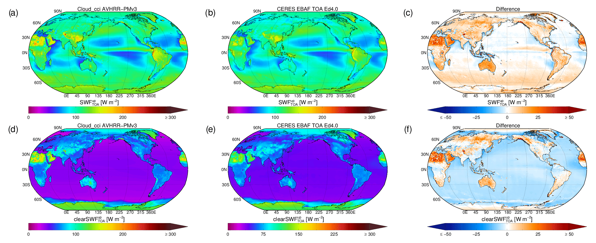
Figure 8 Multi-annual (2003–2016) mean top-of-atmosphere (TOA) upwelling shortwave (SW) radiative fluxes for all-sky conditions for Cloud_cci AVHRR-PMv3 (a) and CERES EBAF TOA Edition 4.0 (b). Panels (d) and (e) show the same data but for clear-sky conditions. Panels (c) and (f) show difference plots Cloud_cci minus CERES.

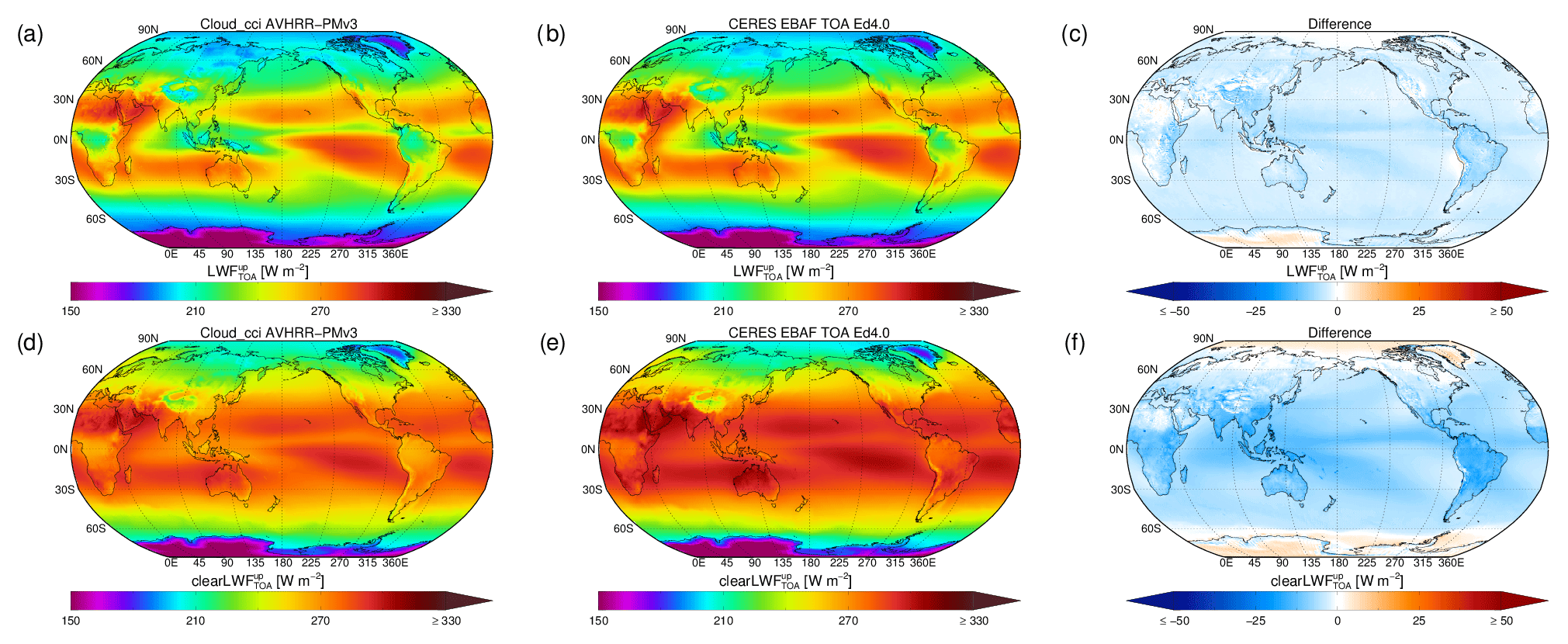
Figure 9 As Fig. 8 but for TOA upwelling longwave (LW) fluxes.

Table 10 Multi-annual (2003–2016), latitude-weighted global mean broadband fluxes at the top of atmosphere (TOA) inferred from Cloud_cci AVHRR-PMv3 dataset for all-sky and clear-sky (clear) conditions. The values are compared to equivalents inferred from Clouds and the Earth's Radiant Energy System (CERES) Energy Balanced and Filled (EBAF) TOA Edition 4.0. All values are given in watts per square metre (W m⁻²). In addition, differences and relative differences (Cloud_cci-CERES) of all fluxes are reported. For comparison, ERA-Interim values are listed as well.

4 Summary

As described in this paper, version 3 of the Cloud_cci AVHRR-PM dataset has been generated (and linked to a DOI; Stengel et al., 2019). In addition to cloud properties, this new version extends the product portfolio by BOA and TOA broadband radiative fluxes and covers the time period 1982 to 2016.

The cloud properties in v3 are superior to v2 in many aspects. This is demonstrated by analyses of global validation results against CALIOP (used for cloud detection, cloud phase and cloud-top height), AMSR-E (used for liquid water path) and DARDAR (combined CALIOP and CloudSat information used for ice water path). Heidke skill scores have increased from 0.64 to 0.68 for cloud detection and from 0.56 to 0.62 for cloud phase assignment. The scores are generally sensitive to whether or not thin clouds are included in the statistical comparisons. The improvements for cloud detection and phase determination in v3 remain conclusive also for scenarios in which very thin clouds are excluded. The validation scores for cloud-top height assignment remain nearly identical for liquid clouds, whereas for ice clouds, lower standard deviations (2.36 km vs. 2.51 km) but larger negative biases (−3.54 km vs. −2.59 km) are found in v3. Similar results are found for scenarios in which the reference height is taken from below the geometrical top, with penetration at optical depths of 0.15 and 1.0. Validation results for liquid water path show a slight reduction in standard deviation for v3 from 27.1 to 26.4 g m⁻², accompanied by a slight increase in bias from −1.9 to −3.2 g m⁻². Correlations remain unchanged at 0.64. Ice water path validation shows reductions of standard deviations for v3 from 1299.8 to 900.9 g m⁻² compared to v2 (reduction by 30 %). While the clearly increased correlation coefficient emphasizes the improvement in v3 as well, the biases are somewhat larger in v3 compared to v2.

A new contribution to version 3 was the addition of top-of-atmosphere and bottom-of-atmosphere broadband radiative fluxes. Validation of v3 monthly mean downwelling radiative fluxes at the BOA against BSRN stations reveals a very good agreement, with low standard deviations of 13.8 W m⁻² for shortwave and 11.5 W m⁻² for longwave fluxes and correlation coefficients above 0.98 for both. While the bias for shortwave fluxes is small (1.9 W m⁻²), a somewhat larger positive bias is found for longwave fluxes (7.6 W m⁻²), which is mainly driven by moderate overestimations of larger flux values in Cloud_cci but can potentially also partly be due to underestimations in the reference (BSRN).

Comparisons of v3 multi-annual mean values of upwelling and downwelling fluxes at the BOA and TOA with CERES additionally emphasize the good quality of the Cloud_cci radiative fluxes in terms of relative spatial pattern and absolute values. Concerning the latter, global mean values of Cloud_cci agree with CERES within 3.3 % for downwelling fluxes at the BOA, with larger deviations found for longwave fluxes. In contrast, Cloud_cci upwelling longwave fluxes at the BOA agree very well with CERES (below 0.5 %), and upwelling shortwave fluxes at the BOA show deviations of up to about 15 %, although the absolute differences are only 4.6 W m⁻² at maximum. It, however, remains uncertain to which extent uncertainties in CERES products contribute to these deviations.

In contrast to the BOA, CERES products for TOA fluxes are mainly based on observational information, thus providing an excellent reference for validation. For all-sky fluxes, Cloud_cci agrees to CERES within 3 % for global mean values. The differences are increased when considering clear-sky fluxes. It is likely that the different approaches to estimate the mean clear-sky fluxes in Cloud_cci (including all conditions but removing the clouds) and CERES (including only cloud-free conditions) contribute considerably to these differences.

In summary, Cloud_cci AVHRR-PMv3 represents a dataset of consistent cloud properties and radiative fluxes, which in many aspects is superior to the precursor version v2 as data quality was improved, the product portfolio extended and the covered time period prolonged. Cloud_cci AVHRR-PMv3 offers a large variety of applications, including climatological analyses of cloud properties and radiative fluxes as well as their dependency on each other at timescales of several decades.

5 Data availability

For the presented dataset (Cloud_cci AVHRR-PMv3), a DOI has been issued: https://doi.org/10.5676/DWD/ESA_Cloud_cci/AVHRR-PM/V003 (Stengel et al., 2019). The landing page points to additional documentation and data download sites. A parallel dataset based on AVHRR aboard the NOAA and EUMETSAT morning satellites exists (AVHRR-AMv3). A DOI has been issued for this as well: https://doi.org/10.5676/DWD/ESA_Cloud_cci/AVHRR-AM/V003. The AVHRR-AMv3 dataset provides the feasibility to be combined with AVHRR-PMv3 to increase sampling frequency. However, for the period of NOAA-12 and NOAA-15 the AVHRR-AMv3 dataset is of reduced quality due to the difficult twilight orbits of NOAA-12 and NOAA-15. The CC4CL retrieval system used to produce the data is version controlled and accessible at GitHub: https://github.com/ORAC-CC/orac/wiki (last access: 12 December 2019). The LUT creation code is available at https://github.com/ORAC-CC/create_orac_lut (last access: 12 December 2019). Both are licensed under the GNU General Public License (GPL) version 3.

Appendix A: AVHRR measurement data

The AVHRR measurement record used as basis for the presented cloud climatology spans the AVHRR-2 and AVHRR-3 sensor generations aboard NOAA-7, NOAA-9, NOAA-11, NOAA-14, NOAA-16, NOAA-18 and NOAA-19. Based on the original AVHRR measurements (Local Area Coverage) with 1 km spatial resolution and sampling distance, the Global Area Coverage (GAC) data are globally available, but with reduced spatial resolution and sampling distance. Only every third scan line is used, and within one scan line four out of five neighbouring pixels are averaged. The AVHRR sensor has an on-board black-body calibration mechanism for its infrared channels. No attempt is made to further recalibrate these measurements. For the visible channels, no calibration is performed aboard AVHRR. A recalibration procedure for these channels was applied as a preparatory step based on Devasthale et al. (2017), with further application aspects reported in Schlundt et al. (2017).

Appendix B: Measurement input to the ANNs and the subsequently applied thresholds

Table B1 Measurement input to the trained artificial neural network for cloud detection (ANN_mask), used for different illumination conditions: daytime, twilight and night-time. The subscript in the table's headline corresponds to the approximate central wavelengths of the channels: 0.6, 0.8, 1.6, 3.7, 10.8 and 12.0 µm. In addition to the measurement input, all ANNs require surface temperature, a snow–ice flag and a land–sea flag as input. R is reflectance, and BT is brightness temperature.

Table B2 Empirical thresholds used to convert the output of the cloud mask ANNs into a binary cloud mask. Thresholds depend on illumination conditions and surface type.

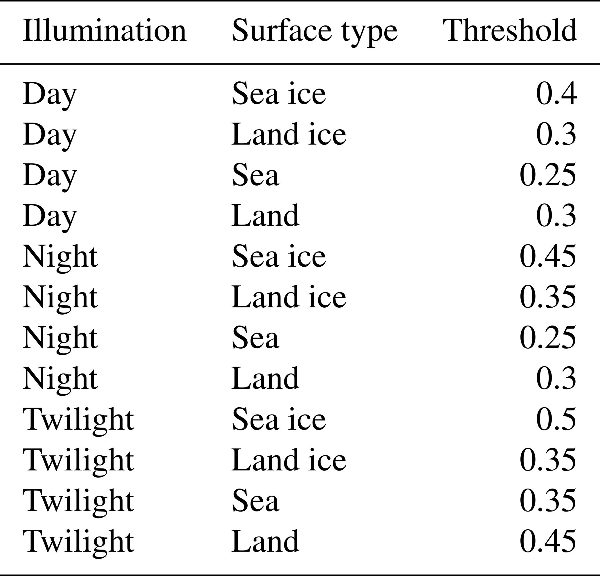
Table B3 Measurement input to the trained artificial neural network for cloud phase determination (ANN_phase), used for different illumination conditions: daytime, twilight and night-time. The subscript in the table's headline corresponds to the approximate central wavelength of the channels: 0.6, 0.8, 1.6, 3.7, 10.8 and 12.0 µm. In addition to the measurement input, all ANNs require a surface type flag containing the values 0 (sea), 1 (land), 2 (desert), 3 (sea ice) and 4 (snow).

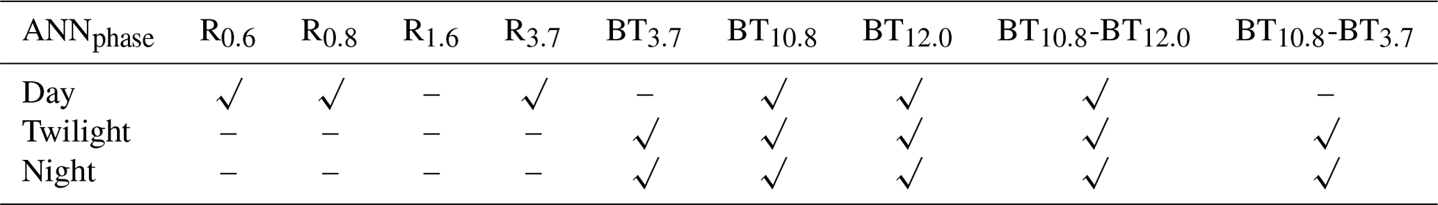
Table B4 Empirical thresholds used to convert the output of the cloud phase ANNs into a binary cloud phase. Thresholds depend on illumination conditions and surface types.

Appendix C: Spectral band adjustment (SBA)

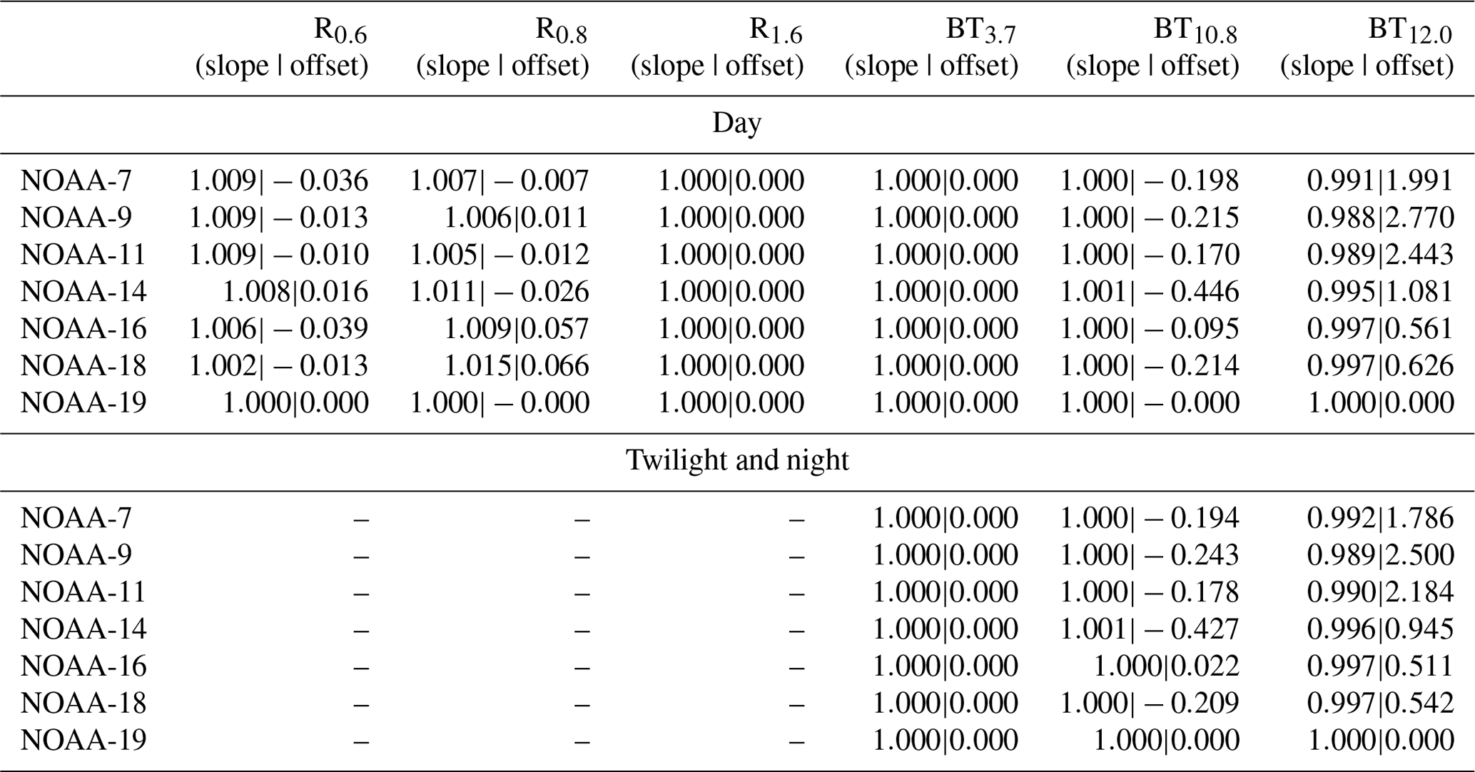
As the cloud detection and cloud phase determination were developed and fine-tuned primarily based on NOAA-19 AVHRR, adjustment factors (slope and offset) were inferred to make all considered AVHRR sensors mimic NOAA-19 AVHRR. The SBAs were inferred from a set of SCIAMACHY and IASI orbits, with both of these sensors providing hyperspectral measurements throughout the visible (SCIAMACHY) and infrared (IASI) part of the spectrum, respectively. Using the spectral response functions (SRFs) of AVHRR channels 0.6, 0.8, 10.8 and 12.0 µm, the SCIAMACHY and IASI measurements were convolved to mimic synthetic AVHRR measurements in each footprint of the considered SCIAMACHY and IASI orbits. Using this procedure for all AVHRR sensors (the AVHRR SRFs differ among the individual satellites) and collecting the synthetic AVHRR measurements in all considered footprints of SCIAMACHY and IASI, a database was composed, allowing for linearly fitting all AVHRR sensors to AVHRR aboard NOAA-19. This SBA is applied prior to the application of the cloud detection and cloud phase procedures. No attempt is made to adjust channels 1.6 and 3.7 µm, as the SCIAMACHY and IASI spectra do not cover the full AVHRR SRF of these channels. All inferred SBAs are given in Table C1. In v2 of the datasets, no SBAs were applied among the AVHRR sensors. As the OE retrieval makes direct use of the SRF of the individual AVHRR sensors, the application of the SBA is not required for the OE retrieval.

Table C1 Linear regression coefficients (slope and offset) applied as spectral-band adjustment to either measured reflectances (Rs) or brightness temperature (BTs) of all used AVHRR channels and all used sensors to mimic NOAA-19 AVHRR. The subscript in the table's headline corresponds to the approximate central wavelengths of the channels: 0.6, 0.8, 1.6, 3.7, 10.8 and 12.0 µm. Reflectances in channels 0.6, 0.8 and 1.6 µm are generally not used in twilight and night conditions.