the Creative Commons Attribution 4.0 License.
the Creative Commons Attribution 4.0 License.
 | 11 Dec 2020
Global Carbon Budget 2020
Pierre Friedlingstein
Michael O'Sullivan
Matthew W. Jones
Robbie M. Andrew
Judith Hauck
Are Olsen
Glen P. Peters
Wouter Peters
Julia Pongratz
Stephen Sitch
Corinne Le Quéré
Josep G. Canadell
Philippe Ciais
Robert B. Jackson
Simone Alin
Luiz E. O. C. Aragão
Almut Arneth
Vivek Arora
Nicholas R. Bates
Meike Becker
Alice Benoit-Cattin
Henry C. Bittig
Laurent Bopp
Selma Bultan
Naveen Chandra
Frédéric Chevallier
Louise P. Chini
Wiley Evans
Liesbeth Florentie
Piers M. Forster
Thomas Gasser
Marion Gehlen
Dennis Gilfillan
Thanos Gkritzalis
Luke Gregor
Nicolas Gruber
Ian Harris
Kerstin Hartung
Vanessa Haverd
Richard A. Houghton
Tatiana Ilyina
Atul K. Jain
Emilie Joetzjer
Koji Kadono
Etsushi Kato
Vassilis Kitidis
Jan Ivar Korsbakken
Peter Landschützer
Nathalie Lefèvre
Andrew Lenton
Sebastian Lienert
Danica Lombardozzi
Gregg Marland
Nicolas Metzl
David R. Munro
Julia E. M. S. Nabel
Shin-Ichiro Nakaoka
Yosuke Niwa
Kevin O'Brien
Tsuneo Ono
Paul I. Palmer
Denis Pierrot
Benjamin Poulter
Laure Resplandy
Eddy Robertson
Christian Rödenbeck
Jörg Schwinger
Roland Séférian
Ingunn Skjelvan
Adam J. P. Smith
Adrienne J. Sutton
Toste Tanhua
Pieter P. Tans
Hanqin Tian
Bronte Tilbrook
Guido van der Werf
Nicolas Vuichard
Anthony P. Walker
Rik Wanninkhof
Andrew J. Watson
David Willis
Andrew J. Wiltshire
Wenping Yuan
Sönke Zaehle
Accurate assessment of anthropogenic carbon dioxide (CO2) emissions and their redistribution among the atmosphere, ocean, and terrestrial biosphere in a changing climate – the “global carbon budget” – is important to better understand the global carbon cycle, support the development of climate policies, and project future climate change. Here we describe and synthesize data sets and methodology to quantify the five major components of the global carbon budget and their uncertainties. Fossil CO2 emissions (EFOS) are based on energy statistics and cement production data, while emissions from land-use change (ELUC), mainly deforestation, are based on land use and land-use change data and bookkeeping models. Atmospheric CO2 concentration is measured directly and its growth rate (GATM) is computed from the annual changes in concentration. The ocean CO2 sink (SOCEAN) and terrestrial CO2 sink (SLAND) are estimated with global process models constrained by observations. The resulting carbon budget imbalance (BIM), the difference between the estimated total emissions and the estimated changes in the atmosphere, ocean, and terrestrial biosphere, is a measure of imperfect data and understanding of the contemporary carbon cycle. All uncertainties are reported as ±1σ. For the last decade available (2010–2019), EFOS was 9.6 ± 0.5 GtC yr−1 excluding the cement carbonation sink (9.4 ± 0.5 GtC yr−1 when the cement carbonation sink is included), and ELUC was 1.6 ± 0.7 GtC yr−1. For the same decade, GATM was 5.1 ± 0.02 GtC yr−1 (2.4 ± 0.01 ppm yr−1), SOCEAN 2.5 ± 0.6 GtC yr−1, and SLAND 3.4 ± 0.9 GtC yr−1, with a budget imbalance BIM of −0.1 GtC yr−1 indicating a near balance between estimated sources and sinks over the last decade. For the year 2019 alone, the growth in EFOS was only about 0.1 % with fossil emissions increasing to 9.9 ± 0.5 GtC yr−1 excluding the cement carbonation sink (9.7 ± 0.5 GtC yr−1 when cement carbonation sink is included), and ELUC was 1.8 ± 0.7 GtC yr−1, for total anthropogenic CO2 emissions of 11.5 ± 0.9 GtC yr−1 (42.2 ± 3.3 GtCO2). Also for 2019, GATM was 5.4 ± 0.2 GtC yr−1 (2.5 ± 0.1 ppm yr−1), SOCEAN was 2.6 ± 0.6 GtC yr−1, and SLAND was 3.1 ± 1.2 GtC yr−1, with a BIM of 0.3 GtC. The global atmospheric CO2 concentration reached 409.85 ± 0.1 ppm averaged over 2019. Preliminary data for 2020, accounting for the COVID-19-induced changes in emissions, suggest a decrease in EFOS relative to 2019 of about −7 % (median estimate) based on individual estimates from four studies of −6 %, −7 %, −7 % (−3 % to −11 %), and −13 %. Overall, the mean and trend in the components of the global carbon budget are consistently estimated over the period 1959–2019, but discrepancies of up to 1 GtC yr−1 persist for the representation of semi-decadal variability in CO2 fluxes. Comparison of estimates from diverse approaches and observations shows (1) no consensus in the mean and trend in land-use change emissions over the last decade, (2) a persistent low agreement between the different methods on the magnitude of the land CO2 flux in the northern extra-tropics, and (3) an apparent discrepancy between the different methods for the ocean sink outside the tropics, particularly in the Southern Ocean. This living data update documents changes in the methods and data sets used in this new global carbon budget and the progress in understanding of the global carbon cycle compared with previous publications of this data set (Friedlingstein et al., 2019; Le Quéré et al., 2018b, a, 2016, 2015b, a, 2014, 2013). The data presented in this work are available at https://doi.org/10.18160/gcp-2020 (Friedlingstein et al., 2020).


The concentration of carbon dioxide (CO2) in the atmosphere has increased from approximately 277 parts per million (ppm) in 1750 (Joos and Spahni, 2008), the beginning of the Industrial Era, to 409.85 ± 0.1 ppm in 2019 (Dlugokencky and Tans, 2020; Fig. 1). The atmospheric CO2 increase above pre-industrial levels was, initially, primarily caused by the release of carbon to the atmosphere from deforestation and other land-use change activities (Ciais et al., 2013). While emissions from fossil fuels started before the Industrial Era, they became the dominant source of anthropogenic emissions to the atmosphere from around 1950 and their relative share has continued to increase until the present. Anthropogenic emissions occur on top of an active natural carbon cycle that circulates carbon between the reservoirs of the atmosphere, ocean, and terrestrial biosphere on timescales from sub-daily to millennia, while exchanges with geologic reservoirs occur at longer timescales (Archer et al., 2009).
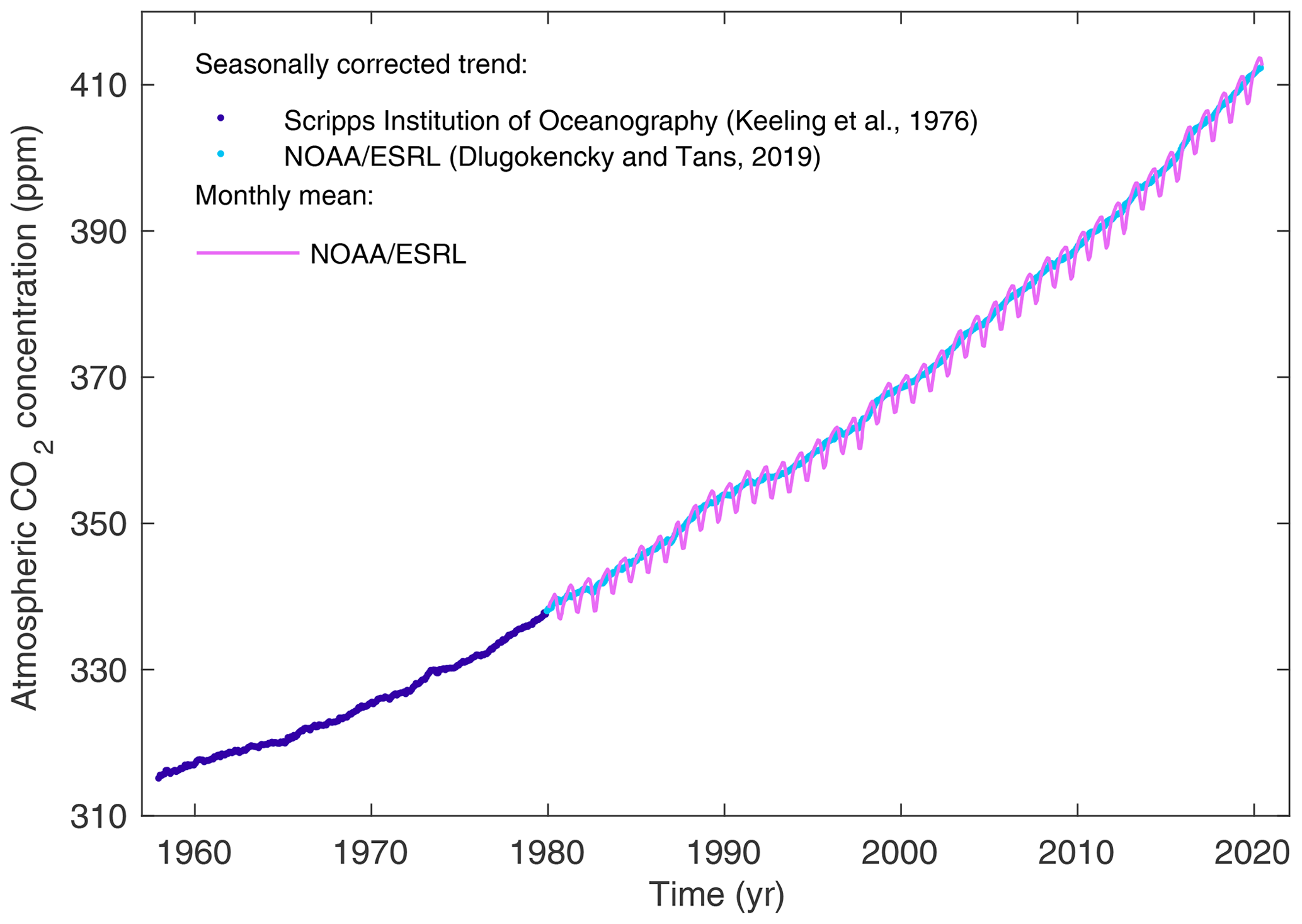
Figure 1Surface average atmospheric CO2 concentration (ppm). The 1980–2019 monthly data are from NOAA/ESRL (Dlugokencky and Tans, 2020) and are based on an average of direct atmospheric CO2 measurements from multiple stations in the marine boundary layer (Masarie and Tans, 1995). The 1958–1979 monthly data are from the Scripps Institution of Oceanography, based on an average of direct atmospheric CO2 measurements from the Mauna Loa and South Pole stations (Keeling et al., 1976). To take into account the difference of mean CO2 and seasonality between the NOAA/ESRL and the Scripps station networks used here, the Scripps surface average (from two stations) was de-seasonalized and harmonized to match the NOAA/ESRL surface average (from multiple stations) by adding the mean difference of 0.542 ppm, calculated here from overlapping data during 1980–2012.
The global carbon budget presented here refers to the mean, variations, and trends in the perturbation of CO2 in the environment, referenced to the beginning of the Industrial Era (defined here as 1750). This paper describes the components of the global carbon cycle over the historical period with a stronger focus on the recent period (since 1958, onset of atmospheric CO2 measurements), the last decade (2010–2019), the last year (2019), and the current year (2020). We quantify the input of CO2 to the atmosphere by emissions from human activities, the growth rate of atmospheric CO2 concentration, and the resulting changes in the storage of carbon in the land and ocean reservoirs in response to increasing atmospheric CO2 levels, climate change and variability, and other anthropogenic and natural changes (Fig. 2). An understanding of this perturbation budget over time and the underlying variability and trends of the natural carbon cycle is necessary to understand the response of natural sinks to changes in climate, CO2, and land-use change drivers, and to quantify the permissible emissions for a given climate stabilization target. Note that this paper quantifies the historical global carbon budget but does not estimate the remaining future carbon emissions consistent with a given climate target, often referred to as the “remaining carbon budget” (Millar et al., 2017; Rogelj et al., 2016, 2019).

Figure 2Schematic representation of the overall perturbation of the global carbon cycle caused by anthropogenic activities, averaged globally for the decade 2010–2019. See legends for the corresponding arrows and units. The uncertainty in the atmospheric CO2 growth rate is very small (±0.02 GtC yr−1) and is neglected for the figure. The anthropogenic perturbation occurs on top of an active carbon cycle, with fluxes and stocks represented in the background and taken from Ciais et al. (2013) for all numbers, with the ocean gross fluxes updated to 90 GtC yr−1 to account for the increase in atmospheric CO2 since publication, and except for the carbon stocks in coasts which is from a literature review of coastal marine sediments (Price and Warren, 2016). Cement carbonation sink of 0.2 GtC yr−1 is included in EFOS.
The components of the CO2 budget that are reported annually in this paper include the following separate estimates for the CO2 emissions: (1) fossil fuel combustion and oxidation from all energy and industrial processes, also including cement production and carbonation (EFOS; GtC yr−1); (2) the emissions resulting from deliberate human activities on land, including those leading to land-use change (ELUC; GtC yr−1); (3) their partitioning among the growth rate of atmospheric CO2 concentration (GATM; GtC yr−1); (4) the sink of CO2 in the ocean (SOCEAN; GtC yr−1); and (5) the sink of CO2 on land (SLAND; GtC yr−1). The CO2 sinks as defined here conceptually include the response of the land (including inland waters and estuaries) and ocean (including coasts and territorial seas) to elevated CO2 and changes in climate, rivers, and other environmental conditions, although in practice not all processes are fully accounted for (see Sect. 2.7). Global emissions and their partitioning among the atmosphere, ocean, and land are in reality in balance. Due to combination of imperfect spatial and/or temporal data coverage, errors in each estimate, and smaller terms not included in our budget estimate (discussed in Sect. 2.7), their sum does not necessarily add up to zero. We estimate a budget imbalance (BIM), which is a measure of the mismatch between the estimated emissions and the estimated changes in the atmosphere, land, and ocean, with the full global carbon budget as follows:
GATM is usually reported in ppm yr−1, which we convert to units of carbon mass per year, GtC yr−1, using 1 ppm = 2.124 GtC (Ballantyne et al., 2012; Table 1). All quantities are presented in units of gigatonnes of carbon (GtC, 1015 gC), which is the same as petagrams of carbon (PgC; Table 1). Units of gigatonnes of CO2 (or billion tonnes of CO2) used in policy are equal to 3.664 multiplied by the value in units of GtC.
Table 1Factors used to convert carbon in various units (by convention, unit 1 = unit 2× conversion).
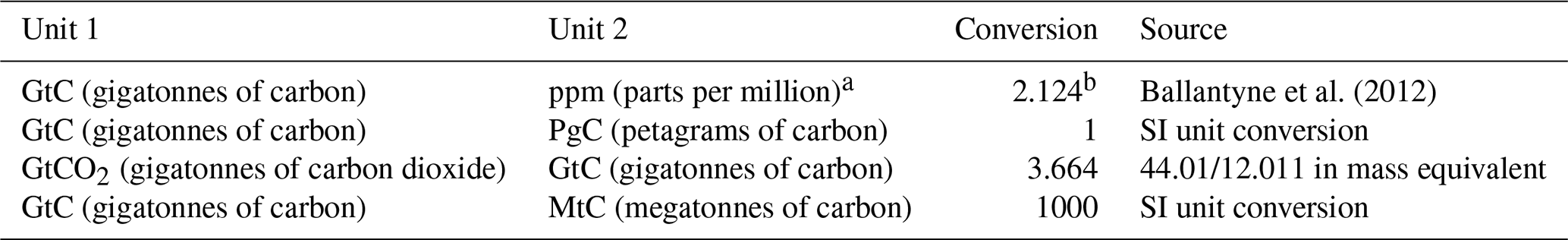
a Measurements of atmospheric CO2 concentration have units of dry-air mole fraction; “ppm” is an abbreviation for micromole mol−1, dry air. b The use of a factor of 2.124 assumes that all the atmosphere is well mixed within 1 year. In reality, only the troposphere is well mixed and the growth rate of CO2 concentration in the less well-mixed stratosphere is not measured by sites from the NOAA network. Using a factor of 2.124 makes the approximation that the growth rate of CO2 concentration in the stratosphere equals that of the troposphere on a yearly basis.
We also include a quantification of EFOS by country, computed with both territorial and consumption-based accounting (see Sect. 2), and discuss missing terms from sources other than the combustion of fossil fuels (see Sect. 2.7).
The global CO2 budget has been assessed by the Intergovernmental Panel on Climate Change (IPCC) in all assessment reports (Prentice et al., 2001; Schimel et al., 1995; Watson et al., 1990; Denman et al., 2007; Ciais et al., 2013), and by others (e.g. Ballantyne et al., 2012). The Global Carbon Project (GCP, https://www.globalcarbonproject.org, last access: 16 November 2020) has coordinated this cooperative community effort for the annual publication of global carbon budgets for the year 2005 (Raupach et al., 2007; including fossil emissions only), year 2006 (Canadell et al., 2007), year 2007 (published online; GCP, 2007), year 2008 (Le Quéré et al., 2009), year 2009 (Friedlingstein et al., 2010), year 2010 (Peters et al., 2012b), year 2012 (Le Quéré et al., 2013; Peters et al., 2013), year 2013 (Le Quéré et al., 2014), year 2014 (Le Quéré et al., 2015a; Friedlingstein et al., 2014), year 2015 (Jackson et al., 2016; Le Quéré et al., 2015b), year 2016 (Le Quéré et al., 2016), year 2017 (Le Quéré et al., 2018a; Peters et al., 2017), year 2018 (Le Quéré et al., 2018b; Jackson et al., 2018), and most recently the year 2019 (Friedlingstein et al., 2019; Jackson et al., 2019; Peters et al., 2020). Each of these papers updated previous estimates with the latest available information for the entire time series.
We adopt a range of ±1 standard deviation (σ) to report the uncertainties in our estimates, representing a likelihood of 68 % that the true value will be within the provided range if the errors have a Gaussian distribution and no bias is assumed. This choice reflects the difficulty of characterizing the uncertainty in the CO2 fluxes between the atmosphere and the ocean and land reservoirs individually, particularly on an annual basis, as well as the difficulty of updating the CO2 emissions from land-use change. A likelihood of 68 % provides an indication of our current capability to quantify each term and its uncertainty given the available information. For comparison, the Fifth Assessment Report of the IPCC (AR5; Ciais et al., 2013) generally reported a likelihood of 90 % for large data sets whose uncertainty is well characterized, or for long time intervals less affected by year-to-year variability. Our 68 % uncertainty value is near the 66 % which the IPCC characterizes as “likely” for values falling into the ±1σ interval. The uncertainties reported here combine statistical analysis of the underlying data and expert judgement of the likelihood of results lying outside this range. The limitations of current information are discussed in the paper and have been examined in detail elsewhere (Ballantyne et al., 2015; Zscheischler et al., 2017). We also use a qualitative assessment of confidence level to characterize the annual estimates from each term based on the type, amount, quality, and consistency of the evidence as defined by the IPCC (Stocker et al., 2013).
This paper provides a detailed description of the data sets and methodology used to compute the global carbon budget estimates for the industrial period, from 1750 to 2019, and in more detail for the period since 1959. It also provides decadal averages starting in 1960 including the most recent decade (2010–2019), results for the year 2019, and a projection for the year 2020. Finally it provides cumulative emissions from fossil fuels and land-use change since the year 1750, the pre-industrial period, and since the year 1850, the reference year for historical simulations in IPCC AR6 (Eyring et al., 2016). This paper is updated every year using the format of “living data” to keep a record of budget versions and the changes in new data, revision of data, and changes in methodology that lead to changes in estimates of the carbon budget. Additional materials associated with the release of each new version will be posted at the GCP website (http://www.globalcarbonproject.org/carbonbudget, last access: 16 November 2020), with fossil fuel emissions also available through the Global Carbon Atlas (http://www.globalcarbonatlas.org, last access: 16 November 2020). With this approach, we aim to provide the highest transparency and traceability in the reporting of CO2, the key driver of climate change.
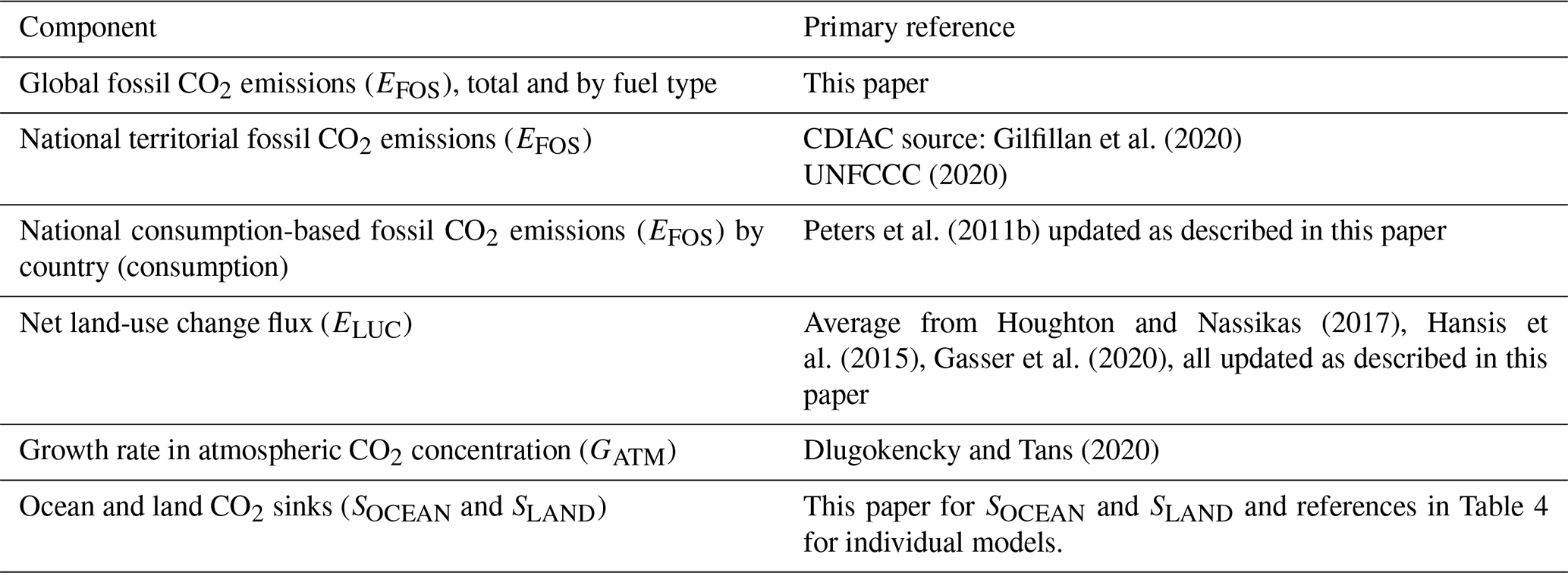
Multiple organizations and research groups around the world generated the original measurements and data used to complete the global carbon budget. The effort presented here is thus mainly one of synthesis, where results from individual groups are collated, analysed, and evaluated for consistency. We facilitate access to original data with the understanding that primary data sets will be referenced in future work (see Table 2 for how to cite the data sets). Descriptions of the measurements, models, and methodologies follow below and detailed descriptions of each component are provided elsewhere.
Table 2How to cite the individual components of the global carbon budget presented here.
This is the 15th version of the global carbon budget and the ninth revised version in the format of a living data update in Earth System Science Data. It builds on the latest published global carbon budget of Friedlingstein et al. (2019). The main changes are (1) the inclusion of data of the year 2019 and a projection for the global carbon budget for year 2020; (2) the inclusion of gross carbon fluxes associated with land-use changes; and (3) the inclusion of cement carbonation in the fossil fuel and cement component of the budget (EFOS). The main methodological differences between recent annual carbon budgets (2015–2019) are summarized in Table 3 and previous changes since 2006 are provided in Table A7.
Table 3Main methodological changes in the global carbon budget since 2016. Methodological changes introduced in one year are kept for the following years unless noted. Empty cells mean there were no methodological changes introduced that year. Table A7 lists methodological changes from the first global carbon budget publication up to 2015.
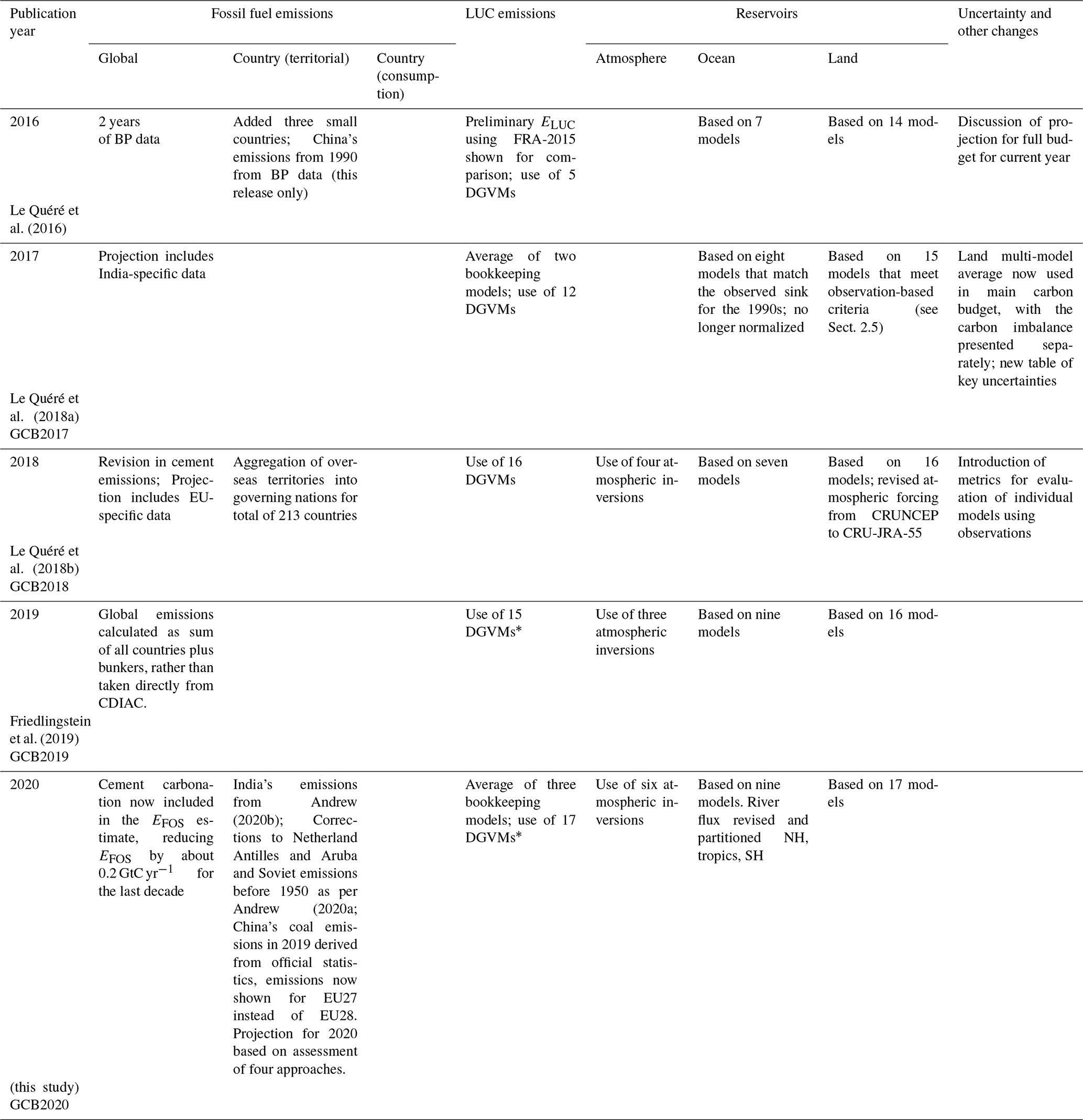
* ELUC is still estimated based on bookkeeping models, as in 2018 (Le Quéré et al., 2018b), but the number of DGVMs used to characterize the uncertainty has changed.
2.1 Fossil CO2 emissions (EFOS)
2.1.1 Emissions estimates
The estimates of global and national fossil CO2 emissions (EFOS) include the combustion of fossil fuels through a wide range of activities (e.g. transport, heating and cooling, industry, fossil industry own use, and natural gas flaring), the production of cement, and other process emissions (e.g. the production of chemicals and fertilizers) as well as CO2 uptake during the cement carbonation process. The estimates of EFOS in this study rely primarily on energy consumption data, specifically data on hydrocarbon fuels, collated and archived by several organizations (Andres et al., 2012; Andrew, 2020a). We use four main data sets for historical emissions (1750–2019):
-
Global and national emission estimates for coal, oil, natural gas, and peat fuel extraction from the Carbon Dioxide Information Analysis Center (CDIAC) for the time period 1750–2017 (Gilfillan et al., 2020), as it is the only data set that extends back to 1750 by country.
-
Official national greenhouse gas inventory reports annually for 1990–2018 for the 42 Annex I countries in the UNFCCC (UNFCCC, 2020). We assess these to be the most accurate estimates because they are compiled by experts within countries that have access to the most detailed data, and they are periodically reviewed.
-
The BP Statistical Review of World Energy (BP, 2020), as these are the most up-to-date estimates of national energy statistics.
-
Global and national cement emissions updated from Andrew (2019) to include the latest estimates of cement production and clinker ratios.
In the following section we provide more details for each data set and describe the additional modifications that are required to make the data set consistent and usable.
CDIAC. The CDIAC estimates have been updated annually up to the year 2017, derived primarily from energy statistics published by the United Nations (UNSD, 2020). Fuel masses and volumes are converted to fuel energy content using country-level coefficients provided by the UN and then converted to CO2 emissions using conversion factors that take into account the relationship between carbon content and energy (heat) content of the different fuel types (coal, oil, natural gas, natural gas flaring) and the combustion efficiency (Marland and Rotty, 1984; Andrew, 2020a). Following Andrew (2020a), we make corrections to emissions from coal in the Soviet Union during World War II, amounting to a cumulative reduction of 53 MtC over 1942–1943, and corrections to emissions from oil in the Netherlands Antilles and Aruba prior to 1950, amounting to a cumulative reduction of 340 MtC over 23 years.
UNFCCC. Estimates from the national greenhouse gas inventory reports submitted to the United Nations Framework Convention on Climate Change (UNFCCC) follow the IPCC guidelines (IPCC, 2006, 2019) but have a slightly larger system boundary than CDIAC by including emissions coming from carbonates other than in cement manufacture. We reallocate the detailed UNFCCC sectoral estimates to the CDIAC definitions of coal, oil, natural gas, cement, and others to allow more consistent comparisons over time and between countries.
Specific country updates. For India, the data reported by CDIAC are for the fiscal year running from April to March (Andrew, 2020a), and various interannual variations in emissions are not supported by official data. Given that India is the world's third-largest emitter and that a new data source is available that resolves these issues, we replace CDIAC estimates with calendar-year estimates through 2019 by Andrew (2020b). For Norway, CDIAC's method of apparent energy consumption results in large errors, and we therefore overwrite emissions before 1990 with estimates derived from official Norwegian statistics.
BP. For the most recent year(s) for which the UNFCCC and CDIAC estimates are not yet available, we generate preliminary estimates using energy consumption data (in exajoules, EJ) from the BP Statistical Review of World Energy (Andres et al., 2014; BP, 2020; Myhre et al., 2009). We apply the BP growth rates by fuel type (coal, oil, natural gas) to estimate 2019 emissions based on 2018 estimates (UNFCCC Annex I countries), and to estimate 2018–2019 emissions based on 2017 estimates (remaining countries except India). BP's data set explicitly covers about 70 countries (96 % of global energy emissions), and for the remaining countries we use growth rates from the sub-region the country belongs to. For the most recent years, natural gas flaring is assumed to be constant from the most recent available year of data (2018 for Annex I countries, 2017 for the remainder). We apply two exceptions to this update using BP data. The first is for China's coal emissions, for which we use growth rates reported in official preliminary statistics for 2019 (NBS, 2020b). The second exception is for Australia, for which BP reports a growth rate of natural gas consumption in Australia of almost 30 %, which is incorrect, and we use a figure of 2.2 % derived from Australia's own reporting (Department of the Environment and Energy, 2020).
Cement. Estimates of emissions from cement production are updated from Andrew (2019). Other carbonate decomposition processes are not included explicitly here, except in national inventories provided by Annex I countries, but are discussed in Sect. 2.7.2.
Country mappings. The published CDIAC data set includes 257 countries and regions. This list includes countries that no longer exist, such as the USSR and Yugoslavia. We reduce the list to 214 countries by reallocating emissions to currently defined territories, using mass-preserving aggregation or disaggregation. Examples of aggregation include merging East and West Germany to the currently defined Germany. Examples of disaggregation include reallocating the emissions from the former USSR to the resulting independent countries. For disaggregation, we use the emission shares when the current territories first appeared (e.g. USSR in 1992), and thus historical estimates of disaggregated countries should be treated with extreme care. In the case of the USSR, we were able to disaggregate 1990 and 1991 using data from the International Energy Agency (IEA). In addition, we aggregate some overseas territories (e.g. Réunion, Guadeloupe) into their governing nations (e.g. France) to align with UNFCCC reporting.
Global total. The global estimate is the sum of the individual countries' emissions and international aviation and marine bunkers. The CDIAC global total differs from the sum of the countries and bunkers since (1) the sum of imports in all countries is not equal to the sum of exports because of reporting inconsistencies, (2) changes in stocks, and (3) the share of non-oxidized carbon (e.g. as solvents, lubricants, feedstocks) at the global level is assumed to be fixed at the 1970s average while it varies in the country-level data based on energy data (Andres et al., 2012). From the 2019 edition CDIAC now includes changes in stocks in the global total (Dennis Gilfillan, personal communication, 2020), removing one contribution to this discrepancy. The discrepancy has grown over time from around zero in 1990 to over 500 MtCO2 in recent years, consistent with the growth in non-oxidized carbon (IEA, 2019). To remove this discrepancy we now calculate the global total as the sum of the countries and international bunkers.
Cement carbonation. From the moment it is created, cement begins to absorb CO2 from the atmosphere, a process known as “cement carbonation”. We estimate this CO2 sink as the average of two studies in the literature (Cao et al., 2020; Guo et al., 2020). Both studies use the same model, developed by Xi et al. (2016), with different parameterizations and input data, with the estimate of Guo and colleagues being a revision of Xi et al. (2016). The trends of the two studies are very similar. Modelling cement carbonation requires estimation of a large number of parameters, including the different types of cement material in different countries, the lifetime of the structures before demolition, of cement waste after demolition, and the volumetric properties of structures, among others (Xi et al., 2016). Lifetime is an important parameter because demolition results in the exposure of new surfaces to the carbonation process. The most significant reasons for differences between the two studies appear to be the assumed lifetimes of cement structures and the geographic resolution, but the uncertainty bounds of the two studies overlap. In the present budget, we include the cement carbonation carbon sink in the fossil CO2 emission component (EFOS), unless explicitly stated otherwise.
2.1.2 Uncertainty assessment for EFOS
We estimate the uncertainty of the global fossil CO2 emissions at ±5 % (scaled down from the published ± 10 % at ±2σ to the use of ±1σ bounds reported here; Andres et al., 2012). This is consistent with a more detailed analysis of uncertainty of ±8.4 % at ±2σ (Andres et al., 2014) and at the high end of the range of ±5 %–10 % at ±2σ reported by Ballantyne et al. (2015). This includes an assessment of uncertainties in the amounts of fuel consumed, the carbon and heat contents of fuels, and the combustion efficiency. While we consider a fixed uncertainty of ±5 % for all years, the uncertainty as a percentage of the emissions is growing with time because of the larger share of global emissions from emerging economies and developing countries (Marland et al., 2009). Generally, emissions from mature economies with good statistical processes have an uncertainty of only a few per cent (Marland, 2008), while emissions from strongly developing economies such as China have uncertainties of around ±10 % (for ±1σ; Gregg et al., 2008; Andres et al., 2014). Uncertainties of emissions are likely to be mainly systematic errors related to underlying biases of energy statistics and to the accounting method used by each country.
2.1.3 Emissions embodied in goods and services
CDIAC, UNFCCC, and BP national emission statistics “include greenhouse gas emissions and removals taking place within national territory and offshore areas over which the country has jurisdiction” (Rypdal et al., 2006) and are called territorial emission inventories. Consumption-based emission inventories allocate emissions to products that are consumed within a country and are conceptually calculated as the territorial emissions minus the “embodied” territorial emissions to produce exported products plus the emissions in other countries to produce imported products (consumption = territorial − exports + imports). Consumption-based emission attribution results (e.g. Davis and Caldeira, 2010) provide additional information to territorial-based emissions that can be used to understand emission drivers (Hertwich and Peters, 2009) and quantify emission transfers by the trade of products between countries (Peters et al., 2011b). The consumption-based emissions have the same global total but reflect the trade-driven movement of emissions across the Earth's surface in response to human activities.
We estimate consumption-based emissions from 1990–2018 by enumerating the global supply chain using a global model of the economic relationships between economic sectors within and between every country (Andrew and Peters, 2013; Peters et al., 2011a). Our analysis is based on the economic and trade data from the Global Trade and Analysis Project (GTAP; Narayanan et al., 2015), and we make detailed estimates for the years 1997 (GTAP version 5) and 2001 (GTAP6) as well as 2004, 2007, and 2011 (GTAP9.2), covering 57 sectors and 141 countries and regions. The detailed results are then extended into an annual time series from 1990 to the latest year of the gross domestic product (GDP) data (2018 in this budget), using GDP data by expenditure in the current exchange rate of US dollars (USD; from the UN National Accounts Main Aggregates Database; UN, 2019) and time series of trade data from GTAP (based on the methodology in Peters et al., 2011b). We estimate the sector-level CO2 emissions using the GTAP data and methodology, include flaring and cement emissions from CDIAC, and then scale the national totals (excluding bunker fuels) to match the emission estimates from the carbon budget. We do not provide a separate uncertainty estimate for the consumption-based emissions, but based on model comparisons and sensitivity analysis, they are unlikely to be significantly different than for the territorial emission estimates (Peters et al., 2012a).
2.1.4 Growth rate in emissions
We report the annual growth rate in emissions for adjacent years (in percent per year) by calculating the difference between the two years and then normalizing to the emissions in the first year: %. We apply a leap-year adjustment where relevant to ensure valid interpretations of annual growth rates. This affects the growth rate by about 0.3 % yr−1 (1∕366) and causes calculated growth rates to go up by approximately 0.3 % if the first year is a leap year and down by 0.3 % if the second year is a leap year.
The relative growth rate of EFOS over time periods of greater than 1 year can be rewritten using its logarithm equivalent as follows:
Here we calculate relative growth rates in emissions for multi-year periods (e.g. a decade) by fitting a linear trend to ln (EFOS) in Eq. (2), reported in percent per year.
2.1.5 Emissions projections
To gain insight into emission trends for 2020, we provide an assessment of global fossil CO2 emissions, EFOS, by combining individual assessments of emissions for China, the USA, the EU, India (the four countries/regions with the largest emissions), and the rest of the world. Our analysis this year is different to previous editions of the Global Carbon Budget, as there have been several independent studies estimating 2020 global CO2 emissions in response to restrictions related to the COVID-19 pandemic, and the highly unusual nature of the year makes the projection much more difficult. We consider three separate studies (Le Quéré et al., 2020; Forster et al., 2020; Liu et al., 2020), in addition to building on the method used in our previous editions. We separate each method into two parts: first we estimate emissions for the year to date (YTD) and, second, we project emissions for the rest of the year 2020. Each method is presented in the order it was published.
UEA: Le Quéré et al. (2020)
YTD. Le Quéré et al. (2020) estimated the effect of COVID-19 on emissions using observed changes in activity using proxy data (such as electricity use, coal use, steel production, road traffic, aircraft departures, etc.), for six sectors of the economy as a function of confinement levels, scaled to the globe based on policy data in response to the pandemic. The analyses employed baseline emissions by country for the latest year available (2018 or 2019) from the Global Carbon Budget 2019 to estimate absolute daily emission changes and covered 67 countries representing 97 % of global emissions. Here we use an update through to 13 November. The parameters for the changes in activity by sector were updated for the industry and aviation sectors, to account for the slow recovery in these sectors observed since the first peak of the pandemic. Specific country-based parameters were used for India and the USA, which improved the match to the observed monthly emissions (from Sect. “Global Carbon Budget Estimates”). By design, this estimate does not include the background seasonal variability in emissions (e.g. lower emissions in Northern Hemisphere summer; Jones et al., 2020), nor the trends in emissions that would be caused by other factors (e.g. reduced use of coal in the EU and the US). To account for the seasonality in emissions where data are available, the mean seasonal variability over 2015–2019 was calculated from available monthly emissions data for the USA, EU27, and India (data from Sect. “Global Carbon Budget Estimates”) and added to the UEA estimate for these regions in Fig. B5. The uncertainty provided reflects the uncertainty in activity parameters.
Projection. A projection is used to fill the data from 14 November to the end of December, assuming countries where confinement measures were at level 1 (targeted measures) on 13 November remain at that level until the end of 2020. For countries where confinement measures were at more stringent levels of 2 and 3 (see Le Quéré et al., 2020) on 13 November, we assume that the measures ease by one level after their announced end date and then remain at that level until the end of 2020.
Priestley Centre: Forster et al. (2020)
YTD. Forster et al. (2020) estimated YTD emissions based primarily on Google mobility data. The mobility data were used to estimate daily fractional changes in emissions from power, surface transport, industry, residential, and public and commercial sectors. The analyses employed baseline emissions for 2019 from the Global Carbon Project to estimate absolute emission changes and covered 123 countries representing over 99 % of global emissions. For a few countries – most notably China and Iran – Google data were not available and so data were obtained from the high-reduction estimate from Le Quéré et al. (2020). We use an updated version of Forster et al. (2020) in which emission-reduction estimates were extended through 3 November.
Projection. The estimates were projected from the start of November to the end of December with the assumption that the declines in emissions from their baselines remain at 66 % of the level over the last 30 d with estimates.
Carbon Monitor: Liu et al. (2020)
YTD. Liu et al. (2020) estimated YTD emissions using emission data and emission proxy activity data including hourly to daily electrical power generation data and carbon emission factors for each different electricity source from the national electricity operation systems of 31 countries, real-time mobility data (TomTom city congestion index data of 416 cities worldwide calibrated to reproduce vehicle fluxes in Paris and FlightRadar24 individual flight location data), monthly industrial production data (calculated separately by cement production, steel production, chemical production, and other industrial production of 27 industries) or indices (primarily the industrial production index) from the national statistics of 62 countries and regions, and monthly fuel consumption data corrected for the daily population-weighted air temperature in 206 countries using predefined heating and temperature functions from EDGAR for residential, commercial, and public buildings' heating emissions, to finally calculate the global fossil CO2 emissions, as well as the daily sectoral emissions from power sector, industry sector, transport sector (including ground transport, aviation, and shipping), and residential sector respectively. We use an updated version of Liu et al. (2020) with data extended through the end of September.
Projection. Liu et al. (2020) did not perform a projection and only presented YTD results. For purposes of comparison with other methods, we use a simple approach to extrapolating their observations by assuming the remaining months of the year change by the same relative amount compared to 2019 in the final month of observations.
Global Carbon Budget estimates
Previous editions of the Global Carbon Budget (GCB) have estimated YTD emissions and performed projections, using sub-annual energy consumption data from a variety of sources depending on the country or region. The YTD estimates have then been projected to the full year using specific methods for each country or region. This year we make some adjustments to this approach, as described below, with detailed descriptions provided in Appendix C.
China. The YTD estimate is based on monthly data from China's National Bureau of Statistics and Customs, with the projection based on the relationship between previous monthly data and full-year data to extend the 2020 monthly data to estimate full-year emissions.
USA. The YTD and projection are taken directly from the US Energy Information Agency.
EU27. The YTD estimates are based on monthly consumption data of coal, oil, and gas converted to CO2 and scaled to match the previous year's emissions. We use the same method for the EU27 as for Carbon Monitor described above to generate a full-year projection.
India. YTD estimates are updated from Andrew (2020b), which calculates monthly emissions directly from detailed energy and cement production data. We use the same method for India as for Carbon Monitor, described above, to generate a full-year projection.
Rest of the world. There is no YTD estimate, while the 2020 projection is based on a GDP estimate from the IMF combined with average improvements in carbon intensity observed in the last 10 years, as in previous editions of the Global Carbon Budget (e.g. Friedlingstein et al., 2019).
Synthesis
In the results section we present the estimates from the four different methods, showing the YTD estimates to the last common historical data point in each data set and the projections for 2020.
2.2 CO2 emissions from land use, land-use change, and forestry (ELUC)
The net CO2 flux from land use, land-use change, and forestry (ELUC, called land-use change emissions in the rest of the text) includes CO2 fluxes from deforestation, afforestation, logging and forest degradation (including harvest activity), shifting cultivation (cycle of cutting forest for agriculture, then abandoning), and regrowth of forests following wood harvest or abandonment of agriculture. Emissions from peat burning and drainage are added from external data sets (see Sect. 2.2.1). Only some land-management activities are included in our land-use change emissions estimates (Table A1). Some of these activities lead to emissions of CO2 to the atmosphere, while others lead to CO2 sinks. ELUC is the net sum of emissions and removals due to all anthropogenic activities considered. Our annual estimate for 1959–2019 is provided as the average of results from three bookkeeping approaches (Sect. 2.2.1): an estimate using the bookkeeping of land use emissions model (Hansis et al., 2015; hereafter BLUE), the estimate published by Houghton and Nassikas (2017; hereafter HandN2017) and the estimate published by Gasser et al. (2020) using the compact Earth system model OSCAR, the latter two updated to 2019. All three data sets are then extrapolated to provide a projection for 2020 (Sect. 2.2.4). In addition, we use results from dynamic global vegetation models (DGVMs; see Sect. 2.2.2 and Table 4) to help quantify the uncertainty in ELUC (Sect. 2.2.3) and thus better characterize our understanding. Note that we use the scientific ELUC definition, which counts fluxes due to environmental changes on managed land towards SLAND, as opposed to the national greenhouse gas inventories under the UNFCCC, which include them in ELUC and thus often report smaller land-use emissions (Grassi et al., 2018; Petrescu et al., 2020).
Table 4References for the process models, pCO2-based ocean flux products, and atmospheric inversions included in Figs. 6–8. All models and products are updated with new data to the end of the year 2019, and the atmospheric forcing for the DGVMs has been updated as described in Sect. 2.2.2.
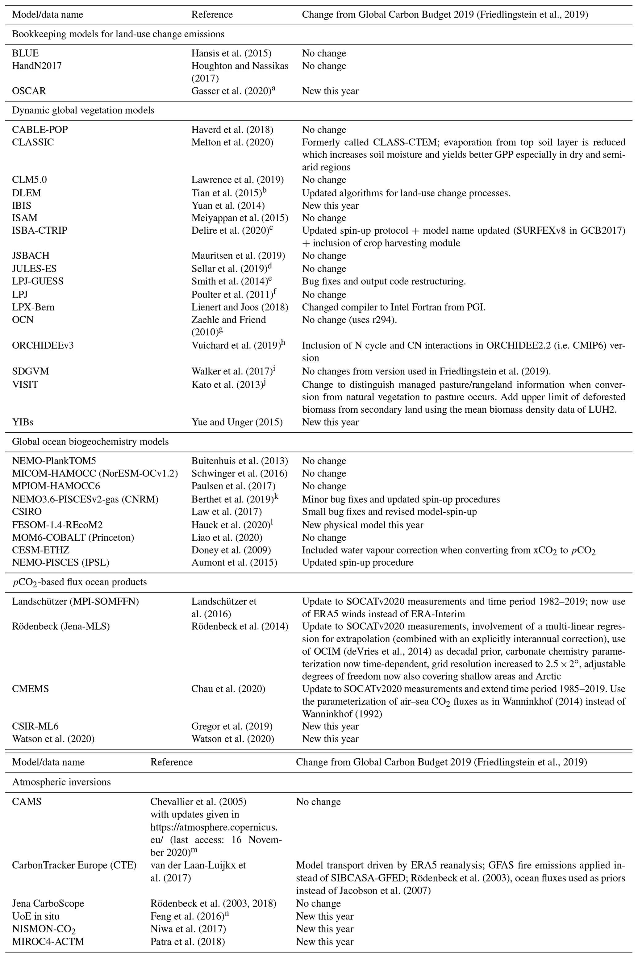
a See also Gasser et al. (2017). b See also Tian et al. (2011). c See also Decharme et al. (2019) and Seferian et al. (2019). d JULES-ES is the Earth System configuration of the Joint UK Land Environment Simulator. See also Best et al. (2011), Clark et al. (2011) and Wiltshire et al. (2020). e To account for the differences between the derivation of shortwave radiation from CRU cloudiness and DSWRF from CRUJRA, the photosynthesis scaling parameter αa was modified (−15 %) to yield similar results. f Lund–Potsdam–Jena. Compared to published version, decreased LPJ wood harvest efficiency so that 50 % of biomass was removed off-site compared to 85 % used in the 2012 budget. Residue management of managed grasslands increased so that 100 % of harvested grass enters the litter pool. g See also Zaehle et al. (2011). h See Zaehle and Friend (2010) and Krinner et al. (2005). i See also Woodward and Lomas (2004). j See also Ito and Inatomi (2012). k See also Seferian et al. (2019). l Longer spin-up than in Hauck et al. (2020); see also Schourup-Kristensen et al. (2014). m See also Remaud et al. (2018). n See also Feng et al. (2009) and Palmer et al. (2019).
2.2.1 Bookkeeping models
Land-use change CO2 emissions and uptake fluxes are calculated by three bookkeeping models. These are based on the original bookkeeping approach of Houghton (2003) that keeps track of the carbon stored in vegetation and soils before and after a land-use change (transitions between various natural vegetation types, croplands, and pastures). Literature-based response curves describe decay of vegetation and soil carbon, including transfer to product pools of different lifetimes, as well as carbon uptake due to regrowth. In addition, the bookkeeping models represent long-term degradation of primary forest as lowered standing vegetation and soil carbon stocks in secondary forests and also include forest management practices such as wood harvests.
BLUE and HandN2017 exclude land ecosystems' transient response to changes in climate, atmospheric CO2, and other environmental factors and base the carbon densities on contemporary data from literature and inventory data. Since carbon densities thus remain fixed over time, the additional sink capacity that ecosystems provide in response to CO2 fertilization and some other environmental changes is not captured by these models (Pongratz et al., 2014). On the contrary, OSCAR includes this transient response, and it follows a theoretical framework (Gasser and Ciais, 2013) that allows separate bookkeeping of land-use emissions and the loss of additional sink capacity. Only the former is included here, while the latter is discussed in Sect. 2.7.4. The bookkeeping models differ in (1) computational units (spatially explicit treatment of land-use change for BLUE, country-level for HandN2017, 10 regions and 5 biomes for OSCAR), (2) processes represented (see Table A1), and (3) carbon densities assigned to vegetation and soil of each vegetation type (literature-based for HandN2017 and BLUE, calibrated to DGVMs for OSCAR). A notable change of HandN2017 over the original approach by Houghton (2003) used in earlier budget estimates is that no shifting cultivation or other back and forth transitions at a level below country are included. Only a decline in forest area in a country as indicated by the Forest Resource Assessment of the FAO that exceeds the expansion of agricultural area as indicated by FAO is assumed to represent a concurrent expansion and abandonment of cropland. In contrast, the BLUE and OSCAR models include sub-grid-scale transitions between all vegetation types. Furthermore, HandN2017 assume conversion of natural grasslands to pasture, while BLUE and OSCAR allocate pasture proportionally on all natural vegetation that exists in a grid cell. This is one reason for generally higher emissions in BLUE and OSCAR. Bookkeeping models do not directly capture carbon emissions from peat fires, which can create large emissions and interannual variability due to synergies of land-use and climate variability in Southeast Asia, in particular during El-Niño events, nor emissions from the organic layers of drained peat soils. To correct for this, HandN2017 includes carbon emissions from peat burning based on the Global Fire Emission Database (GFED4s; van der Werf et al., 2017), and peat drainage based on estimates by Hooijer et al. (2010) for Indonesia and Malaysia. We add GFED4s peat fire emissions to BLUE and OSCAR output but use the newly published global FAO peat drainage emissions 1990–2018 from croplands and grasslands (Conchedda and Tubiello, 2020). We linearly increase tropical drainage emissions from 0 in 1980, consistent with HandN2017's assumption, and keep emissions from the often old drained areas of the extra-tropics constant pre-1990. This adds 8.6 GtC for 1960–2019 for FAO compared to 5.4 GtC for Hooijer et al. (2010). Peat fires add another 2.0 GtC over the same period.
The three bookkeeping estimates used in this study differ with respect to the land-use change data used to drive the models. HandN2017 base their estimates directly on the Forest Resource Assessment of the FAO, which provides statistics on forest-area change and management at intervals of 5 years currently updated until 2015 (FAO, 2015). The data are based on country reporting to FAO and may include remote-sensing information in more recent assessments. Changes in land use other than forests are based on annual, national changes in cropland and pasture areas reported by FAO (FAOSTAT, 2015). On the other hand, BLUE uses the harmonized land-use change data LUH2-GCB2020 covering the entire 850–2019 period (an update to the previously released LUH2 v2h data set; https://doi.org/10.22033/ESGF/input4MIPs.1127; Hurtt et al., 2020), which was also used as input to the DGVMs (Sect. 2.2.2). It describes land-use change, also based on the FAO data as well as the HYDE data set (Klein Goldewijk et al., 2017a, b), but provided at a quarter-degree spatial resolution, considering sub-grid-scale transitions between primary forest, secondary forest, primary non-forest, secondary non-forest, cropland, pasture, rangeland, and urban land (Hurtt et al., 2020). LUH2-GCB2020 provides a distinction between rangelands and pasture, based on inputs from HYDE. To constrain the models' interpretation of whether rangeland implies the original natural vegetation to be transformed to grassland or not (e.g. browsing on shrubland), a forest mask was provided with LUH2-GCB2020; forest is assumed to be transformed to grasslands, while other natural vegetation remains (in case of secondary vegetation) or is degraded from primary to secondary vegetation (Ma et al., 2020). This is implemented in BLUE. OSCAR was run with both LUH2-GCB2019 850–2018 (as used in Friedlingstein et al., 2019) and FAO/FRA (as used by Houghton and Nassikas, 2017), where the latter was extended beyond 2015 with constant 2011–2015 average values. The best-guess OSCAR estimate used in our study is a combination of results for LUH2-GCB2019 and FAO/FRA land-use data and a large number of perturbed parameter simulations weighted against an observational constraint. HandN2017 was extended here for 2016 to 2019 by adding the annual change in total tropical emissions to the HandN2017 estimate for 2015, including estimates of peat drainage and peat burning as described above as well as emissions from tropical deforestation and degradation fires from GFED4.1s (van der Werf et al., 2017). Similarly, OSCAR was extended from 2018 to 2019. Gross fluxes for HandN2017 and OSCAR were extended to 2019 based on a regression of gross sources (including peat emissions) to net emissions for recent years. BLUE's 2019 value was adjusted because the LUH2-GCB2020 forcing for 2019 was an extrapolation of earlier years, thus not capturing the rising deforestation rates occurring in South America in 2019 and the anomalous fire season in equatorial Asia (see Sects. 2.2.4 and 3.2.1). Anomalies of GFED tropical deforestation and degradation and equatorial Asia peat fire emissions relative to 2018 are therefore added. Resulting dynamics in the Amazon are consistent with BLUE simulations using directly observed forest cover loss and forest alert data (Hansen et al., 2013; Hansen et al., 2016).
For ELUC from 1850 onwards we average the estimates from BLUE, HandN2017, and OSCAR. For the cumulative numbers starting 1750 an average of four earlier publications is added (30 ± 20 PgC for 1750–1850, rounded to the nearest 5; Le Quéré et al., 2016).
For the first time we provide estimates of the gross land-use change fluxes from which the reported net land-use change flux, ELUC, is derived as a sum. Gross fluxes are derived internally by the three bookkeeping models: gross emissions stem from decaying material left dead on site and from products after clearing of natural vegetation for agricultural purposes, wood harvesting, emissions from peat drainage and peat burning, and, for BLUE, additionally from degradation from primary to secondary land through usage of natural vegetation as rangeland. Gross removals stem from regrowth after agricultural abandonment and wood harvesting.
2.2.2 Dynamic global vegetation models (DGVMs)
Land-use change CO2 emissions have also been estimated using an ensemble of 17 DGVM simulations. The DGVMs account for deforestation and regrowth, the most important components of ELUC, but they do not represent all processes resulting directly from human activities on land (Table A1). All DGVMs represent processes of vegetation growth and mortality, as well as decomposition of dead organic matter associated with natural cycles, and include the vegetation and soil carbon response to increasing atmospheric CO2 concentration and to climate variability and change. Some models explicitly simulate the coupling of carbon and nitrogen cycles and account for atmospheric N deposition and N fertilizers (Table A1). The DGVMs are independent from the other budget terms except for their use of atmospheric CO2 concentration to calculate the fertilization effect of CO2 on plant photosynthesis.
Many DGVMs used the HYDE land-use change data set (Klein Goldewijk et al., 2017a, b), which provides annual (1700–2019), half-degree, fractional data on cropland and pasture. The data are based on the available annual FAO statistics of change in agricultural land area available until 2015. HYDE version 3.2 used FAO statistics until 2012, which were supplemented using the annual change anomalies from FAO data for the years 2013–2015 relative to year 2012. HYDE forcing was also corrected for Brazil for the years 1951–2012. After the year 2015 HYDE extrapolates cropland, pasture, and urban land-use data until the year 2019. Some models also use the LUH2-GCB2020 data set, an update of the more comprehensive harmonized land-use data set (Hurtt et al., 2011), which further includes fractional data on primary and secondary forest vegetation, as well as all underlying transitions between land-use states (1700–2019) (https://doi.org/10.22033/ESGF/input4MIPs.1127, Hurtt et al., 2017; Hurtt et al., 2011, 2020; Table A1). This new data set is of quarter-degree fractional areas of land-use states and all transitions between those states, including a new wood harvest reconstruction and new representation of shifting cultivation, crop rotations, and management information including irrigation and fertilizer application. The land-use states include five different crop types in addition to the pasture–rangeland split discussed before. Wood harvest patterns are constrained with Landsat-based tree cover loss data (Hansen et al., 2013). Updates of LUH2-GCB2020 over last year's version (LUH2-GCB2019) are using the most recent HYDE/FAO release (covering the time period up to and including 2015), which also corrects an error in the version used for the 2018 budget in Brazil. The FAO wood harvest data have changed for the years 2015 onwards and so those are now being used in this year's LUH-GCB2020 data set. This means the LUH-GCB2020 data are identical to LUH-GCB2019 for all years up to 2015 and differ slightly in terms of wood harvest and resulting secondary area, age, and biomass for years after 2015.
DGVMs implement land-use change differently (e.g. an increased cropland fraction in a grid cell can either be at the expense of grassland or shrubs, or forest, the latter resulting in deforestation; land cover fractions of the non-agricultural land differ between models). Similarly, model-specific assumptions are applied to convert deforested biomass or deforested areas and other forest product pools into carbon, and different choices are made regarding the allocation of rangelands as natural vegetation or pastures.
The DGVM model runs were forced by either the merged monthly Climate Research Unit (CRU) and 6-hourly Japanese 55-year Reanalysis (JRA-55) data set or by the monthly CRU data set, both providing observation-based temperature, precipitation, and incoming surface radiation on a grid and updated to 2019 (Harris and Jones, 2019; Harris et al., 2020). The combination of CRU monthly data with 6-hourly forcing from JRA-55 (Kobayashi et al., 2015) is performed with methodology used in previous years (Viovy, 2016) adapted to the specifics of the JRA-55 data. The forcing data also include global atmospheric CO2, which changes over time (Dlugokencky and Tans, 2020), and gridded, time-dependent N deposition and N fertilizers (as used in some models; Table A1).
Two sets of simulations were performed with each of the DGVMs. Both applied historical changes in climate, atmospheric CO2 concentration, and N inputs. The two sets of simulations differ, however, with respect to land use: one set applies historical changes in land use, the other a time-invariant pre-industrial land cover distribution and pre-industrial wood harvest rates. By difference of the two simulations, the dynamic evolution of vegetation biomass and soil carbon pools in response to land-use change can be quantified in each model (ELUC). Using the difference between these two DGVM simulations to diagnose ELUC means the DGVMs account for the loss of additional sink capacity (see Sect. 2.7.4), while the bookkeeping models do not.
As a criterion for inclusion in this carbon budget, we only retain models that simulate a positive ELUC during the 1990s, as assessed in the IPCC AR4 (Denman et al., 2007) and AR5 (Ciais et al., 2013). All DGVMs met this criteria, although one model was not included in the ELUC estimate from DGVMs as it exhibited a spurious response to the transient land cover change forcing after its initial spin-up.
2.2.3 Uncertainty assessment for ELUC
Differences between the bookkeeping models and DGVM models originate from three main sources: the different methodologies, which among other things lead to inclusion of the loss of additional sink capacity in DGVMs (Sect. 2.7.4), the underlying land-use and land-cover data set, and the different processes represented (Table A1). We examine the results from the DGVM models and of the bookkeeping method and use the resulting variations as a way to characterize the uncertainty in ELUC.
Despite these differences, the ELUC estimate from the DGVM multi-model mean is consistent with the average of the emissions from the bookkeeping models (Table 5). However there are large differences among individual DGVMs (standard deviation at around 0.5 GtC yr−1; Table 5), between the bookkeeping estimates (average difference BLUE-HN2017 of 0.7 GtC yr−1, BLUE-OSCAR of 0.3 GtC yr−1, OSCAR-HN2017 of 0.5 GtC yr−1), and between the current estimate of HandN2017 and its previous model version (Houghton et al., 2012). The uncertainty in ELUC of ±0.7 GtC yr−1 reflects our best-value judgement that there is at least 68 % chance (±1σ) that the true land-use change emission lies within the given range, for the range of processes considered here. Prior to the year 1959, the uncertainty in ELUC was taken from the standard deviation of the DGVMs. We assign low confidence to the annual estimates of ELUC because of the inconsistencies among estimates and of the difficulties in quantifying some of the processes in DGVMs.
Table 5Comparison of results from the bookkeeping method and budget residuals with results from the DGVMs and inverse estimates for different periods, the last decade, and the last year available. All values are in GtC yr−1. The DGVM uncertainties represent ±1σ of the decadal or annual (for 2019 only) estimates from the individual DGVMs: for the inverse models the range of available results is given. All values are rounded to the nearest 0.1 GtC and therefore columns do not necessarily add to zero.
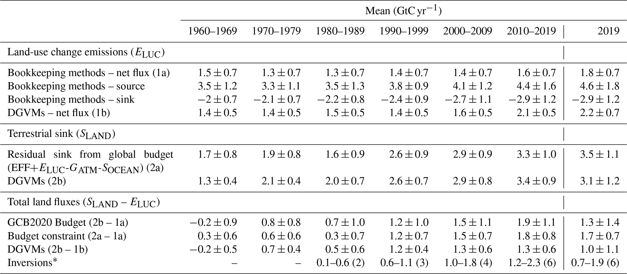
* Estimates are adjusted for the pre-industrial influence of river fluxes and adjusted to common EFOS (Sect. 2.6.1). The ranges given include varying numbers (in parentheses) of inversions in each decade (Table A4).
2.2.4 Emissions projections for ELUC
We project the 2020 land-use emissions for BLUE, HandN2017, and OSCAR, starting from their estimates for 2019 assuming unaltered peat drainage, which has low interannual variability, and the highly variable emissions from peat fires, tropical deforestation, and degradation as estimated using active fire data (MCD14ML; Giglio et al., 2016). Those latter scale almost linearly with GFED over large areas (van der Werf et al., 2017) and thus allow for tracking fire emissions in deforestation and tropical peat zones in near-real time. During most years, emissions during January-September cover most of the fire season in the Amazon and Southeast Asia, where a large part of the global deforestation takes place and our estimates capture emissions until 31 October. By the end of October 2020 emissions from tropical deforestation and degradation fires were estimated to be 227 TgC, down from 347 TgC in 2019 (313 TgC 1997–2019 average). Peat fire emissions in equatorial Asia were estimated to be 1 TgC, down from 117 TgC in 2019 (68 TgC 1997–2019 average). The lower fire emissions for both processes in 2020 compared to 2019 are related to the transition from unusually dry conditions for a non-El Niño year in Indonesia in 2019, which caused relatively high emissions, to few fires due to wet conditions throughout 2020. By contrast, fire emissions in South America remained above-average in 2020, with the slight decrease since 2019 estimated in GFED4.1s (van der Werf et al., 2017) being a conservative estimate. This is consistent with slightly reduced deforestation rates in 2020 compared to 2019 (note that often Amazon deforestation is reported from August of the previous to July of the current year; for such reporting, 2020 deforestation will tend to be higher in 2020 than in 2019 by including strong deforestation August–December 2019). Together, this results in pantropical fire emissions from deforestation, degradation, and peat burning of about 230 TgC projected for 2020 as compared to 464 TgC in 2019; this is slightly above the 2017 and 2018 values of pantropical fire emissions. Overall, however, we have low confidence in our projection due to the large uncertainty range we associate with past ELUC, the dependence of 2020 emissions on legacy fluxes from previous years, uncertainties related to fire emissions estimates, and the lack of data before the end of the year that would allow deforested areas to be quantified accurately. Also, an incomplete coverage of degradation by fire data makes our estimates conservative, considering that degradation rates in the Amazon increased from 2019 to 2020 (INPE, 2020).
2.3 Growth rate in atmospheric CO2 concentration (GATM)
2.3.1 Global growth rate in atmospheric CO2 concentration
The rate of growth of the atmospheric CO2 concentration is provided by the US National Oceanic and Atmospheric Administration Earth System Research Laboratory (NOAA/ESRL; Dlugokencky and Tans, 2020), which is updated from Ballantyne et al. (2012). For the 1959–1979 period, the global growth rate is based on measurements of atmospheric CO2 concentration averaged from the Mauna Loa and South Pole stations, as observed by the CO2 Program at Scripps Institution of Oceanography (Keeling et al., 1976). For the 1980–2019 time period, the global growth rate is based on the average of multiple stations selected from the marine boundary layer sites with well-mixed background air (Ballantyne et al., 2012), after fitting each station with a smoothed curve as a function of time, and averaging by latitude band (Masarie and Tans, 1995). The annual growth rate is estimated by Dlugokencky and Tans (2020) from atmospheric CO2 concentration by taking the average of the most recent December–January months corrected for the average seasonal cycle and subtracting this same average 1 year earlier. The growth rate in units of ppm yr−1 is converted to units of GtC yr−1 by multiplying by a factor of 2.124 GtC ppm−1 (Ballantyne et al., 2012).
The uncertainty around the atmospheric growth rate is due to four main factors: first, the long-term reproducibility of reference gas standards (around 0.03 ppm for 1σ from the 1980s; Dlugokencky and Tans, 2020); second, small unexplained systematic analytical errors that may have a duration of several months to 2 years come and go – they have been simulated by randomizing both the duration and the magnitude (determined from the existing evidence) in a Monte Carlo procedure; third, the network composition of the marine boundary layer with some sites coming or going, gaps in the time series at each site, etc. (Dlugokencky and Tans, 2020) – this uncertainty was estimated by NOAA/ESRL with a Monte Carlo method by constructing 100 “alternative” networks (Masarie and Tans, 1995; NOAA/ESRL, 2020) and added up to 0.085 ppm when summed in quadrature with the second uncertainty (Dlugokencky and Tans, 2020); fourth, the uncertainty associated with using the average CO2 concentration from a surface network to approximate the true atmospheric average CO2 concentration (mass-weighted, in three dimensions) is needed to assess the total atmospheric CO2 burden. In reality, CO2 variations measured at the stations will not exactly track changes in total atmospheric burden, with offsets in magnitude and phasing due to vertical and horizontal mixing. This effect must be very small on decadal and longer timescales, when the atmosphere can be considered well mixed. Preliminary estimates suggest this effect would increase the annual uncertainty, but a full analysis is not yet available. We therefore maintain an uncertainty around the annual growth rate based on the multiple stations' data set ranges between 0.11 and 0.72 GtC yr−1, with a mean of 0.61 GtC yr−1 for 1959–1979 and 0.17 GtC yr−1 for 1980–2019, when a larger set of stations were available as provided by Dlugokencky and Tans (2020), but recognize further exploration of this uncertainty is required. At this time, we estimate the uncertainty of the decadal averaged growth rate after 1980 at 0.02 GtC yr−1 based on the calibration and the annual growth rate uncertainty, but stretched over a 10-year interval. For years prior to 1980, we estimate the decadal averaged uncertainty to be 0.07 GtC yr−1 based on a factor proportional to the annual uncertainty prior and after 1980 ( GtC yr−1).
We assign a high confidence to the annual estimates of GATM because they are based on direct measurements from multiple and consistent instruments and stations distributed around the world (Ballantyne et al., 2012).
In order to estimate the total carbon accumulated in the atmosphere since 1750 or 1850, we use an atmospheric CO2 concentration of 277 ± 3 ppm or 286 ± 3 ppm, respectively, based on a cubic spline fit to ice core data (Joos and Spahni, 2008). The uncertainty of ±3 ppm (converted to ±1σ) is taken directly from the IPCC's assessment (Ciais et al., 2013). Typical uncertainties in the growth rate in atmospheric CO2 concentration from ice core data are equivalent to ±0.1–0.15 GtC yr−1 as evaluated from the Law Dome data (Etheridge et al., 1996) for individual 20-year intervals over the period from 1850 to 1960 (Bruno and Joos, 1997).
2.3.2 Atmospheric growth rate projection
We provide an assessment of GATM for 2020 based on the monthly calculated global atmospheric CO2 concentration (GLO) through August (Dlugokencky and Tans, 2020), and bias-adjusted Holt–Winters exponential smoothing with additive seasonality (Chatfield, 1978) to project to January 2021. Additional analysis suggests that the first half of the year shows more interannual variability than the second half of the year, so that the exact projection method applied to the second half of the year has a relatively smaller impact on the projection of the full year. Uncertainty is estimated from past variability using the standard deviation of the last 5 years' monthly growth rates.
2.4 Ocean CO2 sink
Estimates of the global ocean CO2 sink SOCEAN are from an ensemble of global ocean biogeochemistry models (GOBMs, Table A2) that meet observational constraints over the 1990s (see below). The GOBMs constrain the air–sea CO2 flux by the transport of carbon into the ocean interior, which is also the controlling factor of ocean carbon uptake in the real world. They cover the full globe and all seasons and were recently evaluated against surface ocean pCO2 observations, suggesting they are suitable to estimate the annual ocean carbon sink (Hauck et al., 2020). We use observation-based estimates of SOCEAN to provide a qualitative assessment of confidence in the reported results, and two diagnostic ocean models to estimate SOCEAN over the industrial era (see below).
2.4.1 Observation-based estimates
We primarily use the observational constraints assessed by IPCC of a mean ocean CO2 sink of 2.2 ± 0.7 GtC yr−1 for the 1990s (90 % confidence interval; Ciais et al., 2013) to verify that the GOBMs provide a realistic assessment of SOCEAN. We further test that GOBMs and data products fall within the IPCC estimates for the 2000s (2.3 ± 0.7 GtC yr−1) and the period 2002–2011 (2.4 ± 0.7 GtC yr−1; Ciais et al., 2013). The IPCC estimates are based on the observational constraint of the mean 1990s sink and trends derived mainly from models and one data product (Ciais et al., 2013). This is based on indirect observations with seven different methodologies and their uncertainties, using the methods that are deemed most reliable for the assessment of this quantity (Denman et al., 2007; Ciais et al., 2013). The observation-based estimates use the ocean–land CO2 sink partitioning from observed atmospheric CO2 and O2∕N2 concentration trends (Manning and Keeling, 2006; Keeling and Manning, 2014), an oceanic inversion method constrained by ocean biogeochemistry data (Mikaloff Fletcher et al., 2006), and a method based on penetration timescales for chlorofluorocarbons (McNeil et al., 2003). The IPCC estimate of 2.2 GtC yr−1 for the 1990s is consistent with a range of methods (Wanninkhof et al., 2013).
We also use four estimates of the ocean CO2 sink and its variability based on surface ocean pCO2 maps obtained by the interpolation of measurements of surface ocean fugacity of CO2 (fCO2, which equals pCO2 corrected for the non-ideal behaviour of the gas; Pfeil et al., 2013). These estimates differ in many respects: they use different maps of surface pCO2, different atmospheric CO2 concentrations, wind products, and different gas-exchange formulations as specified in Table A3. We refer to them as pCO2-based flux estimates. The measurements underlying the surface pCO2 maps are from the Surface Ocean CO2 Atlas version 2020 (SOCATv2020; Bakker et al., 2020), which is an update of version 3 (Bakker et al., 2016) and contains quality-controlled data through 2019 (see data attribution Table A5). Each of the estimates uses a different method to then map the SOCAT v2020 data to the global ocean. The methods include a data-driven diagnostic method (Rödenbeck et al., 2013; referred to here as Jena-MLS), a combined self-organizing map and feed-forward neural network (Landschützer et al., 2014; referred to here as MPI-SOMFFN), an artificial neural network model (Denvil-Sommer et al., 2019; Copernicus Marine Environment Monitoring Service, referred to here as CMEMS), and an ensemble average of six machine learning estimates of pCO2 using a cluster regression approach (Gregor et al., 2019; referred to here as CSIR). The ensemble mean of the pCO2-based flux estimates is calculated from these four mapping methods. Further, we show the flux estimate of Watson et al. (2020) whose uptake is substantially larger, owing to a number of adjustments they applied to the surface ocean fCO2 data and the gas-exchange parameterization. Concretely, these authors adjusted the SOCAT fCO2 downward to account for differences in temperature between the depth of the ship intake and the relevant depth right near the surface and also included a further adjustment to account for the cool surface skin temperature effect. They then used the MPI-SOMFFN method to map the adjusted fCO2 data to the globe. The Watson et al. (2020) flux estimate hence differs from the others by their choice of adjusting the flux to a cool, salty ocean surface skin. Watson et al. (2020) showed that this temperature adjustment leads to an upward correction of the ocean carbon sink, up to 0.9 GtC yr−1, which, if correct, should be applied to all pCO2-based flux estimates. So far this adjustment is based on a single line of evidence and hence associated with low confidence until further evidence is available. The Watson et al. (2020) flux estimate presented here is therefore not included in the ensemble mean of the pCO2-based flux estimates. This choice will be re-evaluated in upcoming budgets based on further lines of evidence.
The global pCO2-based flux estimates were adjusted to remove the pre-industrial ocean source of CO2 to the atmosphere of 0.61 GtC yr−1 from river input to the ocean (the average of 0.45 ± 0.18 GtC yr−1 by Jacobson et al. ,2007, and 0.78 ± 0.41 GtC yr−1 by Resplandy et al., 2018), to satisfy our definition of SOCEAN (Hauck et al., 2020). The river flux adjustment was distributed over the latitudinal bands using the regional distribution of Aumont et al. (2001; north: 0.16 GtC yr−1, tropics: 0.15 GtC yr−1, south: 0.30 GtC yr−1). The CO2 flux from each pCO2-based product is scaled by the ratio of the total ocean area covered by the respective product to the total ocean area (361.9×10⁶ km2) from ETOPO1 (Amante and Eakins, 2009; Eakins and Sharman, 2010). In products where the covered area varies with time (MPI-SOMFFN, CMEMS) we use the maximum area coverage. The data products cover 88 % (MPI-SOMFFN, CMEMS) to 101 % (Jena-MLS) of the observed total ocean area, so two products are effectively corrected upwards by a factor of 1.13 (Table A3, Hauck et al., 2020).
We further use results from two diagnostic ocean models, Khatiwala et al. (2013) and DeVries (2014), to estimate the anthropogenic carbon accumulated in the ocean prior to 1959. The two approaches assume constant ocean circulation and biological fluxes, with SOCEAN estimated as a response in the change in atmospheric CO2 concentration calibrated to observations. The uncertainty in cumulative uptake of ±20 GtC (converted to ±1σ) is taken directly from the IPCC's review of the literature (Rhein et al., 2013), or about ±30 % for the annual values (Khatiwala et al., 2009).
2.4.2 Global ocean biogeochemistry models (GOBMs)
The ocean CO2 sink for 1959–2019 is estimated using nine GOBMs (Table A2). The GOBMs represent the physical, chemical, and biological processes that influence the surface ocean concentration of CO2 and thus the air–sea CO2 flux. The GOBMs are forced by meteorological reanalysis and atmospheric CO2 concentration data available for the entire time period. They mostly differ in the source of the atmospheric forcing data (meteorological reanalysis), spin-up strategies, and in their horizontal and vertical resolutions (Table A2). All GOBMs except one (CESM-ETHZ) do not include the effects of anthropogenic changes in nutrient supply (Duce et al., 2008). They also do not include the perturbation associated with changes in riverine organic carbon (see Sect. 2.7.3).
Two sets of simulations were performed with each of the GOBMs. Simulation A applied historical changes in climate and atmospheric CO2 concentration. Simulation B is a control simulation with constant atmospheric forcing (normal year or repeated-year forcing) and constant pre-industrial atmospheric CO2 concentration. In order to derive SOCEAN from the model simulations, we subtracted the annual time series of the control simulation B from the annual time series of simulation A. Assuming that drift and bias are the same in simulations A and B, we thereby correct for any model drift. Further, this difference also removes the natural steady state flux (assumed to be 0 GtC yr−1 globally) which is often a major source of biases. Simulation B of IPSL had to be treated differently as it was forced with constant atmospheric CO2 but observed historical changes in climate. For IPSL, we fitted a linear trend to the simulation B and subtracted this linear trend from simulation A. This approach ensures that the interannual variability is not removed from IPSL simulation A.
The absolute correction for bias and drift per model in the 1990s varied between < 0.01 and 0.35 GtC yr−1, with six models having positive and three models having negative biases. This correction reduces the model mean ocean carbon sink by 0.07 GtC yr−1 in the 1990s. The CO2 flux from each model is scaled by the ratio of the total ocean area covered by the respective GOBM to the total ocean area (361.9×10⁶ km2) from ETOPO1 (Amante and Eakins, 2009; Eakins and Sharman, 2010). The ocean models cover 99 % to 101 % of the total ocean area, so the effect of this correction is small.
2.4.3 GOBM evaluation and uncertainty assessment for SOCEAN
The mean ocean CO2 sink for all GOBMs and the ensemble mean falls within 90 % confidence of the observed range, or 1.5 to 2.9 GtC yr−1 for the 1990s (Ciais et al., 2013) and within the derived constraints for the 2000s and 2002–2011 (see Sect. 2.4.1) before and after applying corrections. The GOBMs and flux products have been further evaluated using the fugacity of sea surface CO2 (fCO2) from the SOCAT v2020 database (Bakker et al., 2016, 2020). The fugacity of CO2 is 3 ‰–4 ‰ smaller than the partial pressure of CO2 (Zeebe and Wolf-Gladrow, 2001). We focused this evaluation on the root mean squared error (RMSE) between observed fCO2 and modelled pCO2 and on a measure of the amplitude of the interannual variability of the flux (modified after Rödenbeck et al., 2015). The RMSE is calculated from annually and regionally averaged time series calculated from GOBM and data product pCO2 subsampled to open ocean (water depth > 400 m) SOCAT sampling points to measure the misfit between large-scale signals (Hauck et al., 2020) as opposed to the RMSE calculated from binned monthly data as in the previous year. The amplitude of the SOCEAN interannual variability (A-IAV) is calculated as the temporal standard deviation of the detrended CO2 flux time series (Rödenbeck et al., 2015; Hauck et al., 2020). These metrics are chosen because RMSE is the most direct measure of data–model mismatch and the A-IAV is a direct measure of the variability of SOCEAN on interannual timescales. We apply these metrics globally and by latitude bands (Fig. B1). Results are shown in Fig. B1 and discussed in Sect. 3.1.3.
The 1σ uncertainty around the mean ocean sink of anthropogenic CO2 was quantified by Denman et al. (2007) for the 1990s to be ±0.5 GtC yr−1. Here we scale the uncertainty of ±0.5 GtC yr−1 to the mean estimate of 2.2 GtC yr−1 in the 1990s to obtain a relative uncertainty of ± 18 %, which is then applied to the full time series. To quantify the uncertainty around annual values, we examine the standard deviation of the GOBM ensemble, which varies between 0.2 and 0.4 GtC yr−1 and averages to 0.30 GtC yr−1 during 1959–2019. We estimate that the uncertainty in the annual ocean CO2 sink increases from ±0.3 GtC yr−1 in the 1960s to ±0.6 GtC yr−1 in the decade 2010–2019 from the combined uncertainty of the mean flux based on observations of ±18 % (Denman et al., 2007) and the standard deviation across GOBMs of up to ±0.4 GtC yr−1, reflecting both the uncertainty in the mean sink from observations during the 1990s (Denman et al., 2007; Sect. 2.4.1) and the uncertainty in annual estimates from the standard deviation across the GOBM ensemble.
We examine the consistency between the variability of the model-based and the pCO2-based flux products to assess confidence in SOCEAN. The interannual variability of the ocean fluxes (quantified as A-IAV, the standard deviation after detrending; Fig. B1) of the four pCO2-based flux products plus the Watson et al. (2020) product for 1992–2019 ranges from 0.16 to 0.25 GtC yr−1 with the lower estimates by the two ensemble methods (CSIR, CMEMS). The inter-annual variability in the GOBMs ranges between 0.11 and 0.17 GtC yr−1; hence there is overlap with the lower A-IAV estimates of two data products.
Individual estimates (both GOBM and flux products) generally produce a higher ocean CO2 sink during strong El Niño events. There is emerging agreement between GOBMs and data products on the patterns of decadal variability of SOCEAN with a global stagnation in the 1990s and an extra-tropical strengthening in the 2000s (McKinley et al., 2020; Hauck et al., 2020).
The annual pCO2-based flux products correlate with the ocean CO2 sink estimated here with a correlation coefficient r ranging from 0.80 to 0.97 (1985–2019). The central estimates of the annual flux from the GOBMs and the pCO2-based flux products have a correlation r of 0.97 (1985–2019). The agreement between the models and the flux products reflects some consistency in their representation of underlying variability since there is little overlap in their methodology or use of observations. We assess a medium confidence level to the annual ocean CO2 sink and its uncertainty because it is based on multiple lines of evidence, it is consistent with ocean interior carbon estimates (Gruber et al., 2019; see Sect. 3.1.2), and the results are consistent in that the interannual variability in the GOBMs and data-based estimates are all generally small compared to the variability in the growth rate of atmospheric CO2 concentration.
2.5 Terrestrial CO2 sink
2.5.1 DGVM simulations
The terrestrial land sink (SLAND) is thought to be due to the combined effects of fertilization by rising atmospheric CO2 and N inputs on plant growth, as well as the effects of climate change such as the lengthening of the growing season in northern temperate and boreal areas. SLAND does not include land sinks directly resulting from land use and land-use change (e.g. regrowth of vegetation) as these are part of the land-use flux (ELUC), although system boundaries make it difficult to attribute CO2 fluxes on land exactly between SLAND and ELUC (Erb et al., 2013).
SLAND is estimated from the multi-model mean of 17 DGVMs (Table 4). As described in Sect. 2.2.2, DGVM simulations include all climate variability and CO2 effects over land, with 12 DGVMs also including the effect of N inputs. The DGVMs estimate of SLAND does not include the export of carbon to aquatic systems or its historical perturbation, which is discussed in Sect. 2.7.3.
2.5.2 DGVM evaluation and uncertainty assessment for SLAND
We apply three criteria for minimum DGVM realism by including only those DGVMs with (1) steady state after spin-up; (2) global net land flux (SLAND – ELUC) that is an atmosphere-to-land carbon flux over the 1990s ranging between −0.3 and 2.3 GtC yr−1, within 90 % confidence of constraints by global atmospheric and oceanic observations (Keeling and Manning, 2014; Wanninkhof et al., 2013); and (3) global ELUC that is a carbon source to the atmosphere over the 1990s, as already mentioned in Sect. 2.2.2. All 17 DGVMs meet these three criteria.
In addition, the DGVM results are also evaluated using the International Land Model Benchmarking system (ILAMB; Collier et al., 2018). This evaluation is provided here to document, encourage, and support model improvements through time. ILAMB variables cover key processes that are relevant for the quantification of SLAND and resulting aggregated outcomes. The selected variables are vegetation biomass, gross primary productivity, leaf area index, net ecosystem exchange, ecosystem respiration, evapotranspiration, soil carbon, and runoff (see Fig. B2 for the results and for the list of observed databases). Results are shown in Fig. B2 and discussed in Sect. 3.1.3.
For the uncertainty for SLAND, we use the standard deviation of the annual CO2 sink across the DGVMs, averaging to about ±0.6 GtC yr−1 for the period 1959 to 2019. We attach a medium confidence level to the annual land CO2 sink and its uncertainty because the estimates from the residual budget and averaged DGVMs match well within their respective uncertainties (Table 5).
2.6 The atmospheric inversion perspective
The worldwide network of in situ atmospheric measurements and satellite-derived atmospheric CO2 column (xCO2) observations can be used with atmospheric inversion methods to constrain the location of the combined total surface CO2 fluxes from all sources, including fossil and land-use change emissions and land and ocean CO2 fluxes. The inversions assume EFOS to be well known, and they solve for the spatial and temporal distribution of land and ocean fluxes from the residual gradients of CO2 between stations that are not explained by fossil fuel emissions.
Six atmospheric inversions (Table A4) used atmospheric CO2 data to the end of 2019 (including preliminary values in some cases) to infer the spatio-temporal distribution of the CO2 flux exchanged between the atmosphere and the land or oceans. We focus here on the total land and ocean CO2 fluxes and their partitioning among the northern extra-tropics (30–90∘ N), the tropics (30∘ S–30∘ N), and the southern extra-tropics (30–90∘ S). We also break down those estimates for the land and ocean regions separately. We use these estimates to comment on the consistency across various data streams and process-based estimates.
The six inversion systems used in this release are described in Table A4. The inversions are based on Bayesian inversion principles with prior information on fluxes and their uncertainties. The inversion systems are based on near-identical observations of surface measurements of CO2 time series (or subsets thereof) from various flask and in situ networks. Two inversion systems (University of Edinburgh, UoE, and CAMS) were also applied using only satellite xCO2 measurements from GOSAT or OCO-2, but their results at the larger scales discussed in this work did not deviate substantially from their in situ counterparts and are therefore not separately included (Palmer et al., 2019). Each inversion system uses different methodologies and input data but is rooted in Bayesian inversion principles (Table A4). These differences mainly concern the selection of atmospheric CO2 data and prior fluxes, as well as the spatial resolution, assumed correlation structures, and mathematical approach of the models. The details of each model's approach are documented extensively in the references provided in Table A4. Each system uses a different transport model, which was demonstrated to be a driving factor behind differences in atmospheric inversion-based flux estimates, and specifically their distribution across latitudinal bands (Gaubert et al., 2019; Schuh et al., 2019).
The inversion systems prescribe global fossil fuel emissions. For the first time in this year's budget, most (five of the six) inversion systems prescribed the same estimate for EFOS, specifically the GCP's Gridded Fossil Emissions Dataset version 2020.1 (GCP-GridFEDv2020.1), which is an update to 2019 of the first version of GCP-GridFED presented by Jones et al. (2020). GCP-GridFEDv2020.1 scales gridded estimates of CO2 emissions from EDGARv4.3.2 (Janssens-Maenhout et al., 2019) within national territories to match national emissions estimates provided by the GCP for the years 1959–2019, which were compiled following the methodology described in Sect. 2.1 with all data sets available on 31 July 2020 (Robbie Andrew, personal communication, 2020).
A new feature in this edition of the global carbon budget is the use of a consistent prior emissions data set for EFOS across almost all inversion models, which avoids the need to correct the estimated land sink (by up to 0.5 GtC in the northern extra-tropics) for most models. Only the UoE inversion used an alternative data set and required a post-processing correction (see Table A4). Further, the use of GCP-GridFEDv2020.1 for EFOS ensures a close alignment with the estimate of EFOS used in this budget assessment, enhancing the comparability of the inversion-based estimate with the flux estimates deriving from DGVMs, GOBMs, and pCO2-based methods.
The land and ocean CO2 fluxes from atmospheric inversions contain anthropogenic perturbation and natural pre-industrial CO2 fluxes. On annual timescales, natural pre-industrial fluxes are primarily land CO2 sinks and ocean CO2 sources corresponding to carbon taken up on land, transported by rivers from land to ocean, and outgassed by the ocean. These pre-industrial land CO2 sinks are thus compensated over the globe by ocean CO2 sources corresponding to the outgassing of riverine carbon inputs to the ocean. We apply the distribution of land-to-ocean C fluxes from rivers in three latitude bands using estimates from Resplandy et al. (2018), which are constrained by ocean heat transport to a total land-to-ocean carbon transfer of 0.61 GtC yr−1. The latitude distribution of river-induced ocean CO2 sources (north: 0.16 GtC yr−1, tropics: 0.15 GtC yr−1, south: 0.30 GtC yr−1) from carbon originating from land (north: 0.29 GtC yr−1, tropics: 0.32 GtC yr−1, south: < 0.01 GtC yr−1) is derived by scaling the outgassing per latitude band from Aumont et al. (2001) to the global estimate of 0.61 GtC yr−1. To facilitate the comparison, we adjusted the inverse estimates of the land and ocean fluxes per latitude band with these numbers to produce historical perturbation CO2 fluxes from inversions.
The atmospheric inversions are also evaluated using vertical profiles of atmospheric CO2 concentrations (Fig. B3). More than 30 aircraft programs over the globe, either regular programs or repeated surveys over at least 9 months, have been used in order to draw a robust picture of the model performance (with space–time data coverage irregular and denser in the 0–45∘ N latitude band; Table A6). The six models are compared to the independent aircraft CO2 measurements between 2 and 7 km above sea level between 2001 and 2018. Results are shown in Fig. B3 and discussed in Sect. 3.1.3.
2.7 Processes not included in the global carbon budget
The contribution of anthropogenic CO and CH4 to the global carbon budget is not fully accounted for in Eq. (1) and is described in Sect. 2.7.1. The contribution of other carbonates to CO2 emissions is described in Sect. 2.7.2. The contribution of anthropogenic changes in river fluxes is conceptually included in Eq. (1) in SOCEAN and in SLAND, but it is not represented in the process models used to quantify these fluxes. This effect is discussed in Sect. 2.7.3. Similarly, the loss of additional sink capacity from reduced forest cover is missing in the combination of approaches used here to estimate both land fluxes (ELUC and SLAND), and its potential effect is discussed and quantified in Sect. 2.7.4.
2.7.1 Contribution of anthropogenic CO and CH4 to the global carbon budget
Equation (1) only partly includes the net input of CO2 to the atmosphere from the chemical oxidation of reactive carbon-containing gases from sources other than the combustion of fossil fuels, such as (1) cement process emissions, since these do not come from combustion of fossil fuels; (2) the oxidation of fossil fuels; and (3) the assumption of immediate oxidation of vented methane in oil production. It omits, however, any other anthropogenic carbon-containing gases that are eventually oxidized in the atmosphere, such as anthropogenic emissions of CO and CH4. An attempt is made in this section to estimate their magnitude and identify the sources of uncertainty. Anthropogenic CO emissions are from incomplete fossil fuel and biofuel burning and deforestation fires. The main anthropogenic emissions of fossil CH4 that matter for the global (anthropogenic) carbon budget are the fugitive emissions of coal, oil, and gas sectors (see below). These emissions of CO and CH4 contribute a net addition of fossil carbon to the atmosphere.
In our estimate of EFOS we assumed (Sect. 2.1.1) that all the fuel burned is emitted as CO2, and thus CO anthropogenic emissions associated with incomplete fossil fuel combustion and its atmospheric oxidation into CO2 within a few months are already counted implicitly in EFOS and should not be counted twice (same for ELUC and anthropogenic CO emissions by deforestation fires). Anthropogenic emissions of fossil CH4 are, however, not included in EFOS, because these fugitive emissions are not included in the fuel inventories. Yet they contribute to the annual CO2 growth rate after CH4 gets oxidized into CO2. Emissions of fossil CH4 represent 30 % of total anthropogenic CH4 emissions (Saunois et al., 2020; their top-down estimate is used because it is consistent with the observed CH4 growth rate), which is 0.083 GtC yr−1 for the decade 2008–2017. Assuming a steady state, an amount equal to this fossil CH4 emission is all converted to CO2 by OH oxidation and thus explains 0.083 GtC yr−1 of the global CO2 growth rate with an uncertainty range of 0.061 to 0.098 GtC yr−1 taken from the minimum and maximum of top-down estimates in Saunois et al. (2020). If this minimum–maximum range is assumed to be 2σ because Saunois et al. (2020) did not account for the internal uncertainty of their min and max top-down estimates, it translates into a 1σ uncertainty of 0.019 GtC yr−1.
Other anthropogenic changes in the sources of CO and CH4 from wildfires, vegetation biomass, wetlands, ruminants, or permafrost changes are similarly assumed to have a small effect on the CO2 growth rate. The CH4 and CO emissions and sinks are published and analysed separately in the Global Methane Budget and Global Carbon Monoxide Budget publications, which follow a similar approach to that presented here (Saunois et al., 2020; Zheng et al., 2019).
2.7.2 Contribution of other carbonates to CO2 emissions
This year we account for cement carbonation (a carbon sink) for the first time. The contribution of emissions of fossil carbonates (carbon sources) other than cement production is not systematically included in estimates of EFOS, except at the national level where they are accounted for in the UNFCCC national inventories. The missing processes include CO2 emissions associated with the calcination of lime and limestone outside cement production. Carbonates are also used in various industries, including in iron and steel manufacture and in agriculture. They are found naturally in some coals. CO2 emissions from fossil carbonates other than cement are estimated to amount to about 1 % of EFOS (Crippa et al., 2019), though some of these carbonate emissions are included in our estimates (e.g. via UNFCCC inventories).
2.7.3 Anthropogenic carbon fluxes in the land-to-ocean aquatic continuum
The approach used to determine the global carbon budget refers to the mean, variations, and trends in the perturbation of CO2 in the atmosphere, referenced to the pre-industrial era. Carbon is continuously displaced from the land to the ocean through the land–ocean aquatic continuum (LOAC) comprising freshwaters, estuaries, and coastal areas (Bauer et al., 2013; Regnier et al., 2013). A significant fraction of this lateral carbon flux is entirely “natural” and is thus a steady state component of the pre-industrial carbon cycle. We account for this pre-industrial flux where appropriate in our study. However, changes in environmental conditions and land-use change have caused an increase in the lateral transport of carbon into the LOAC – a perturbation that is relevant for the global carbon budget presented here.
The results of the analysis of Regnier et al. (2013) can be summarized in two points of relevance for the anthropogenic CO2 budget. First, the anthropogenic perturbation of the LOAC has increased the organic carbon export from terrestrial ecosystems to the hydrosphere by as much as 1.0 ± 0.5 GtC yr−1 since pre-industrial times, mainly owing to enhanced carbon export from soils. Second, this exported anthropogenic carbon is partly respired through the LOAC, partly sequestered in sediments along the LOAC, and to a lesser extent transferred to the open ocean where it may accumulate or be outgassed. The increase in storage of land-derived organic carbon in the LOAC carbon reservoirs (burial) and in the open ocean combined is estimated by Regnier et al. (2013) to be 0.65 ± 0.35 GtC yr−1. The inclusion of LOAC-related anthropogenic CO2 fluxes should affect estimates of SLAND and SOCEAN in Eq. (1) but does not affect the other terms. Representation of the anthropogenic perturbation of LOAC CO2 fluxes is, however, not included in the GOBMs and DGVMs used in our global carbon budget analysis presented here.
2.7.4 Loss of additional sink capacity
Historical land-cover change was dominated by transitions from vegetation types that can provide a large carbon sink per area unit (typically, forests) to others less efficient in removing CO2 from the atmosphere (typically, croplands). The resultant decrease in land sink, called the “loss of additional sink capacity”, can be calculated as the difference between the actual land sink under changing land cover and the counterfactual land sink under pre-industrial land cover. This term is not accounted for in our global carbon budget estimate. Here, we provide a quantitative estimate of this term to be used in the discussion. Seven of the DGVMs used in Friedlingstein et al. (2019) performed additional simulations with and without land-use change under cycled pre-industrial environmental conditions. The resulting loss of additional sink capacity amounts to 0.9 ± 0.3 GtC yr−1 on average over 2009–2018 and 42 ± 16 GtC accumulated between 1850 and 2018. OSCAR, emulating the behaviour of 11 DGVMs, finds values of the loss of additional sink capacity of 0.7 ± 0.6 GtC yr−1 and 31 ± 23 GtC for the same time period (Gasser et al., 2020). Since the DGVM-based ELUC estimates are only used to quantify the uncertainty around the bookkeeping models' ELUC we do not add the loss of additional sink capacity to the bookkeeping estimate.
3.1 Global carbon budget mean and variability for 1959–2019
The global carbon budget averaged over the historical period (1850–2019) is shown in Fig. 3. For the more recent 1959–2019 period where direct atmospheric CO2 measurements are available, 81 % of the total emissions (EFOS+ELUC) were caused by fossil CO2 emissions, and 19 % by land-use change. The total emissions were partitioned among the atmosphere (45 %), ocean (24 %), and land (32 %), with a near-zero unattributed budget imbalance (0 %). All components except land-use change emissions have significantly grown since 1959, with important interannual variability in the growth rate in atmospheric CO2 concentration and in the land CO2 sink (Fig. 4), and some decadal variability in all terms (Table 6). Differences with previous budget releases are documented in Fig. B4.
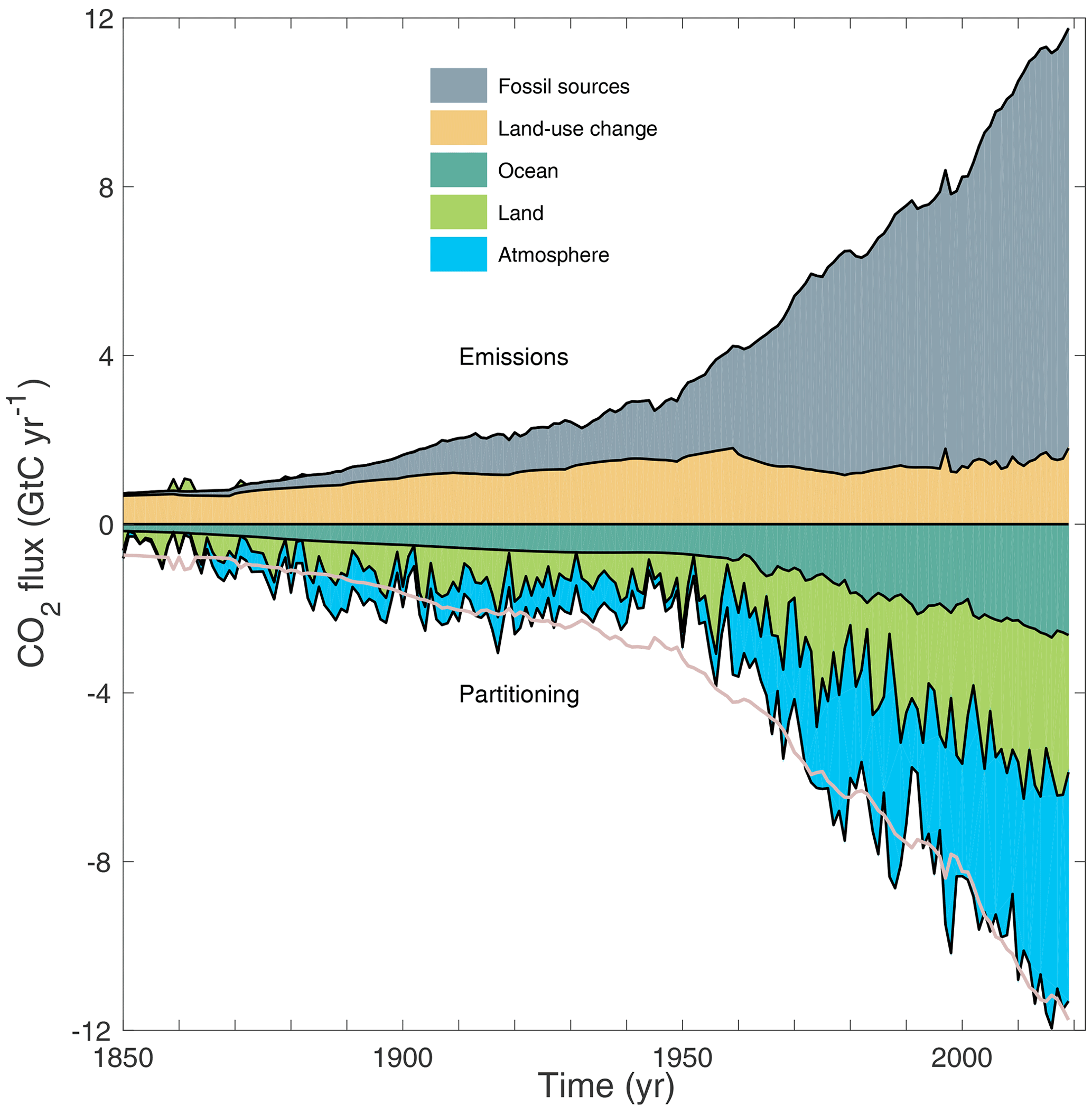
Figure 3Combined components of the global carbon budget illustrated in Fig. 2 as a function of time, for fossil CO2 emissions (EFOS, including a small sink from cement carbonation; grey) and emissions from land-use change (ELUC; brown), as well as their partitioning among the atmosphere (GATM; blue), ocean (SOCEAN; turquoise), and land (SLAND; green). The partitioning is based on nearly independent estimates from observations (for GATM) and from process model ensembles constrained by data (for SOCEAN and SLAND) and does not exactly add up to the sum of the emissions, resulting in a budget imbalance which is represented by the difference between the bottom pink line (reflecting total emissions) and the sum of the ocean, land, and atmosphere. All time series are in GtC yr−1. GATM and SOCEAN prior to 1959 are based on different methods. EFOS values are primarily from Gilfillan et al. (2020), with uncertainty of about ±5 % (±1σ). ELUC values are from two bookkeeping models (Table 2) with uncertainties of about ± 50 %. GATM prior to 1959 is from Joos and Spahni (2008) with uncertainties equivalent to about ±0.1–0.15 GtC yr−1, and from Dlugokencky and Tans (2020) from 1959 with uncertainties of about ±0.2 GtC yr−1. SOCEAN prior to 1959 is averaged from Khatiwala et al. (2013) and DeVries (2014) with uncertainty of about ±30 %, and from a multi-model mean (Table 4) from 1959 with uncertainties of about ±0.5 GtC yr−1. SLAND is a multi-model mean (Table 4) with uncertainties of about ±0.9 GtC yr−1. See the text for more details of each component and their uncertainties.
Table 6Decadal mean in the five components of the anthropogenic CO2 budget for different periods, and last year available. All values are in GtC yr−1, and uncertainties are reported as ±1σ. The table also shows the budget imbalance (BIM), which provides a measure of the discrepancies among the nearly independent estimates and has an uncertainty exceeding ±1 GtC yr−1. A positive imbalance means the emissions are overestimated and/or the sinks are too small. All values are rounded to the nearest 0.1 GtC and therefore columns do not necessarily add to zero.
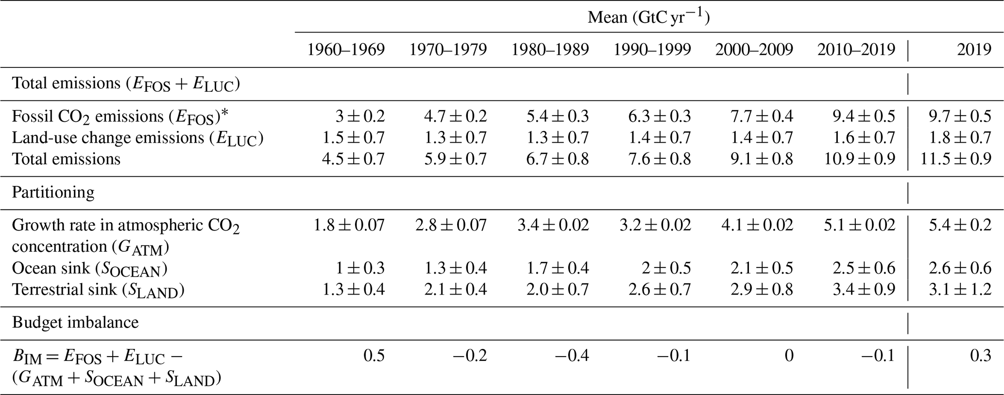
∗ Fossil emissions excluding the cement carbonation sink amount to 3.0 ± 0.2 GtC yr−1, 4.7 ± 0.2 GtC yr−1, 5.5 ± 0.3 GtC yr−1, 6.4 ± 0.3 GtC yr−1, 7.8 ± 0.4 GtC yr−1, and 9.6 ± 0.5 GtC yr−1 for the decades 1960s to 2010s respectively and to 9.9 ± 0.5 GtC yr−1 for 2019.
3.1.1 CO2 emissions
Global fossil CO2 emissions have increased every decade from an average of 3.0 ± 0.2 GtC yr−1 for the decade of the 1960s to an average of 9.4 ± 0.5 GtC yr−1 during 2010–2019 (Table 6, Figs. 2 and 5). The growth rate in these emissions decreased between the 1960s and the 1990s, from 4.3 % yr−1 in the 1960s (1960–1969), 3.1 % yr−1 in the 1970s (1970–1979), 1.6 % yr−1 in the 1980s (1980–1989), to 0.9 % yr−1 in the 1990s (1990–1999). After this period, the growth rate began increasing again in the 2000s at an average growth rate of 3.0 % yr−1, decreasing to 1.2 % yr−1 for the last decade (2010–2019).
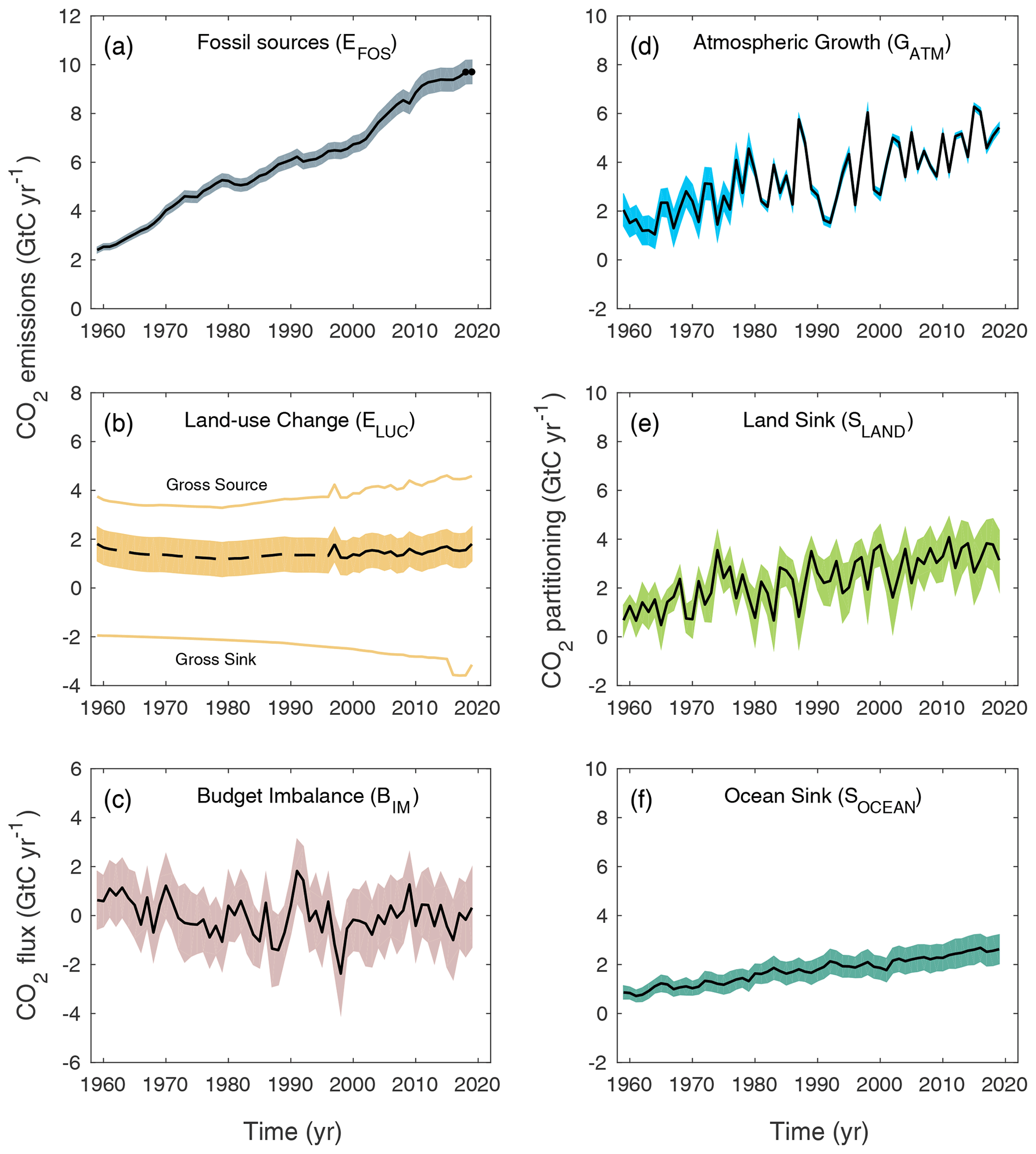
Figure 4Components of the global carbon budget and their uncertainties as a function of time, presented individually for (a) fossil CO2 emissions including cement carbonation sink (EFOS), (b) emissions from land-use change (ELUC), (c) the budget imbalance that is not accounted for by the other terms,(d) growth rate in atmospheric CO2 concentration (GATM), (e) the land CO2 sink (SLAND, positive indicates a flux from the atmosphere to the land), and (f) the ocean CO2 sink (SOCEAN, positive indicates a flux from the atmosphere to the ocean). All time series are in GtC yr−1 with the uncertainty bounds representing ±1σ in shaded colour. Data sources are as in Fig. 3. The black dots in (a) show values for 2018–2019 that originate from a different data set to the remainder of the data (see text). The dashed line in (b) identifies the pre-satellite period before the inclusion of emissions from peatland burning.
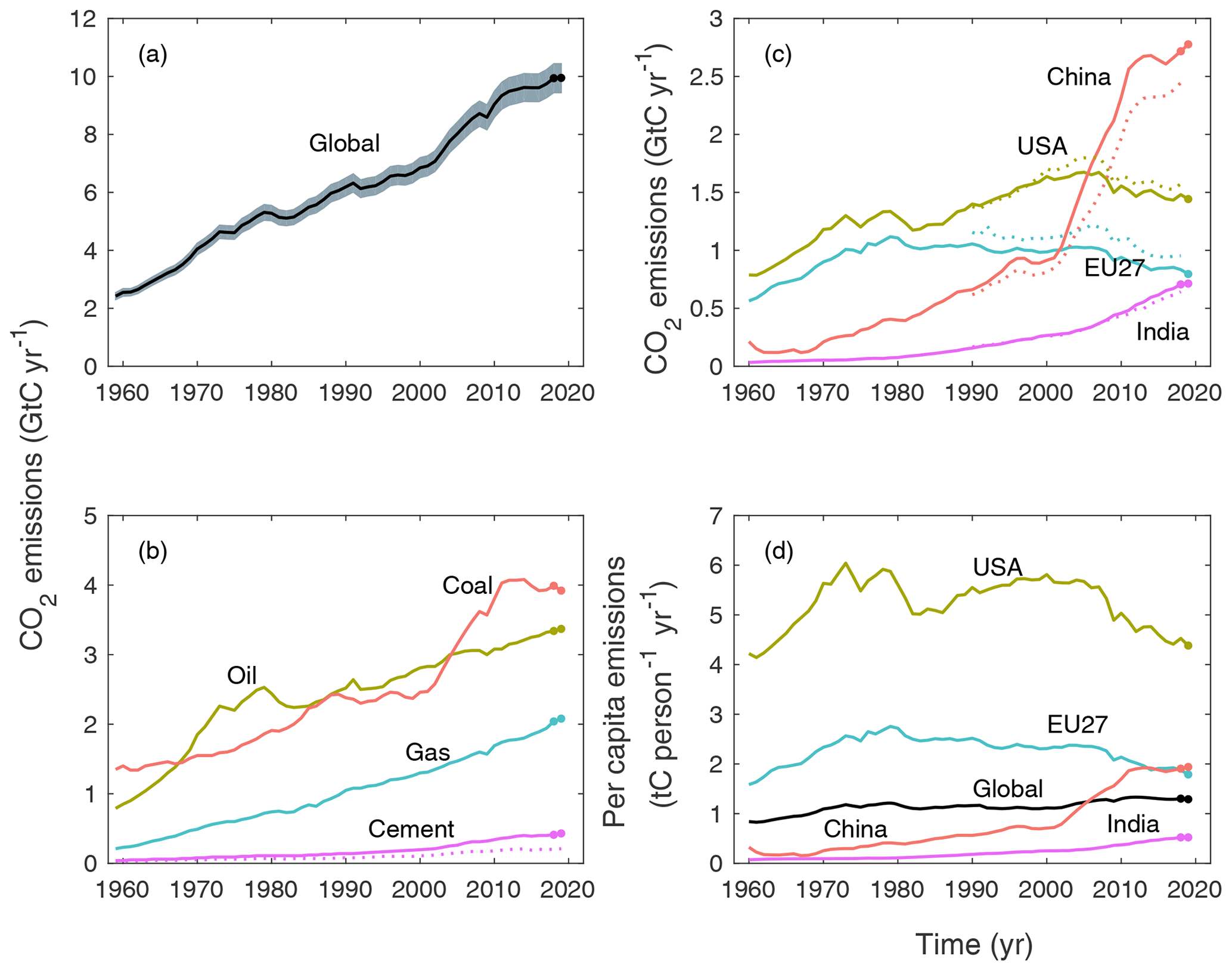
Figure 5Fossil CO2 emissions for (a) the globe, including an uncertainty of ±5 % (grey shading), and the emissions extrapolated using BP energy statistics (black dots); (b) global emissions by categories, including coal (salmon), oil (olive), gas (turquoise), cement production (purple), and cement production minus carbonation sink (dotted purple), and excluding gas flaring which is small (0.6 % in 2013); (c) territorial (solid lines) and consumption (dashed lines) emissions for the top three emitter countries (USA – olive; China – salmon; India – purple) and for the European Union (EU; turquoise for the 27 member states of the EU as of 2020); and (d) per capita emissions for the top three emitter countries and the EU (all colours as in panel c) and the world (black). In (b)–(c), the dots show the data that were extrapolated from BP energy statistics for 2018–2019. All time series are in GtC yr−1 except the per capita emissions (d), which are in tonnes of carbon per person per year (tC per person per year). Territorial emissions are primarily from Gilfillan et al. (2020) except national data for the USA and EU27 (the 27 member states of the EU) for 1990–2018, which are reported by the countries to the UNFCCC as detailed in the text; consumption-based emissions are updated from Peters et al. (2011a). See Sect. 2.1.1 for details of the calculations and data sources.
In contrast, CO2 emissions from land use, land-use change, and forestry have remained relatively constant, at around 1.4 ± 0.7 GtC yr−1 over the past half-century (Table 6) but with large spread across estimates (Table 5, Fig. 6). These emissions are also relatively constant in the DGVM ensemble of models, except during the last decade when they increase to 2.1 ± 0.5 GtC yr−1. However, there is no agreement on this recent increase between the bookkeeping estimates, with HandN2017 suggesting a downward trend as compared to a weak and strong upward trend in OSCAR and the BLUE estimates respectively (Fig. 6).
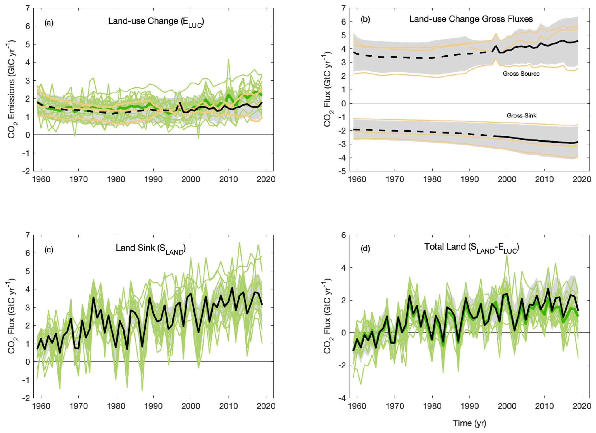
Figure 6CO2 exchanges between the atmosphere and the terrestrial biosphere as used in the global carbon budget (black with ±1σ uncertainty in grey shading), for (a) CO2 emissions from land-use change (ELUC). Estimates from the three bookkeeping models (brown lines) and the DGVM models (green) are shown individually, as is the multi-model mean of DGVM models (dark green). The dashed line identifies the pre-satellite period before the inclusion of peatland burning. (b) CO2 gross sinks (from regrowth after agricultural abandonment and wood harvesting) and gross sources (decaying material left dead on site and from products after clearing of natural vegetation for agricultural purposes, wood harvesting, and, for BLUE, degradation from primary to secondary land through usage of natural vegetation as rangeland, and emissions from peat drainage and peat burning). The sum of the gross sinks and sources is ELUC. Estimates from the three bookkeeping models (brown lines) are shown individually. (c) Land CO2 sink (SLAND) with individual DGVMs (green). (d) Total land CO2 fluxes (c minus a) with individual DGVMs (green) and their multi-model mean (dark green).
ELUC is a net term of various gross fluxes, which comprise emissions and removals (see Sect. 2.2.1). Gross emissions are on average 2–3 times larger than the net ELUC emissions, increasing from an average of 3.5 ± 1.2 GtC yr−1 for the decade of the 1960s to an average of 4.4 ± 1.6 GtC yr−1 during 2010–2019 (Fig. 6, Table 5), showing the relevance of land management such as harvesting or rotational agriculture. They differ more across the three bookkeeping estimates than net fluxes, which is expected due to different process representation; in particular explicit inclusion of shifting cultivation (BLUE, OSCAR) increases both gross emissions and removals.
The uptake of CO2 by cement via carbonation has increased with increasing stocks of cement products, from an average of 20 MtC yr−1 in the 1960s to an average of 190 MtC yr−1 during 2010–2019 (Fig. 5). The growth rate declined from 6.7 % yr−1 in the 1960s to 3.3 % yr−1 in the 1980s, rising again to 6.2 % yr−1 in the 2000s, before declining again to 3.5 % yr−1 in the 2010s.
3.1.2 Partitioning among the atmosphere, ocean, and land
The growth rate in atmospheric CO2 level increased from 1.8 ± 0.07 GtC yr−1 in the 1960s to 5.1 ± 0.02 GtC yr−1 during 2010–2019 with important decadal variations (Table 6 and Fig. 3). Both ocean and land CO2 sinks have increased roughly in line with the atmospheric increase, but with significant decadal variability on land (Table 6 and Fig. 6), and possibly in the ocean (Fig. 7).
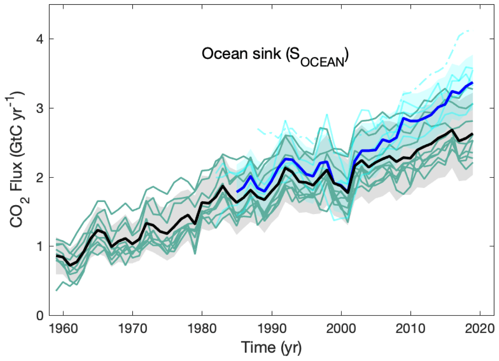
Figure 7Comparison of the anthropogenic atmosphere–ocean CO2 flux showing the budget values of SOCEAN (black; with ±1σ uncertainty in grey shading), individual ocean models (teal), and the ocean pCO2-based flux products (ensemble mean in dark blue, with ±1σ uncertainty in light blue shading – see Table 4; individual products in cyan; Watson et al. (2020) as a dashed–dotted line not used for ensemble mean). The pCO2-based flux products were adjusted for the pre-industrial ocean source of CO2 from river input to the ocean, which is not present in the ocean models, by adding a sink of 0.61 GtC yr−1 to make them comparable to SOCEAN (see Sect. 2.7.3).
The ocean CO2 sink increased from 1.0 ± 0.3 GtC yr−1 in the 1960s to 2.5 ± 0.6 GtC yr−1 during 2010–2019, with interannual variations of the order of a few tenths of GtC yr−1 generally showing an increased ocean sink during large El Niño events (i.e. 1997–1998) (Fig. 7; Rödenbeck et al., 2014; Hauck et al., 2020). The GOBMs show the same patterns of decadal variability as the mean of the pCO2-based flux products, but of weaker magnitude (Sect. 2.4.3 and Fig. 7; DeVries et al., 2019; Hauck et al., 2020). The pCO2-based flux products and the ocean inverse model highlight different regions as the main origin of this decadal variability, with the pCO2-based flux products placing more of the weakening trend in the Southern Ocean and the ocean inverse model suggesting that more of the weakening trend occurred in the North Atlantic and North Pacific (DeVries et al., 2019). Both approaches also show decadal trends in the low-latitude oceans (DeVries et al., 2019).
Although all individual GOBMs and data products fall within the observational constraint, the ensemble means of GOBMs and data products adjusted for the riverine flux diverge over time with a mean offset of 0.15 GtC yr−1 in the 1990s to 0.55 GtC yr−1 in the decade 2010–2019 and ≥ 0.70 GtC yr−1 since 2017. The GOBMs' best estimate of SOCEAN over the period 1994–2007 is 2.1 ± 0.5 GtC yr−1 and is in agreement with the ocean interior estimate of 2.2 ± 0.4 GtC yr−1 when taking into account the interior ocean carbon changes of 2.6 ± 0.3 GtC yr−1 due to the increase in atmospheric CO2 and −0.4 ± 0.24 GtC yr−1 due to anthropogenic climate change and variability effects on the natural CO2 flux (Gruber et al., 2019) to match the definition of SOCEAN used here (Hauck et al., 2020). The discrepancy between GOBMs and data products stems from the southern and northern extra-tropics prior to 2005, and mostly from the Southern Ocean since the mid-2000s. Possible explanations for the discrepancy in the Southern Ocean could be missing winter observations or uncertainties in the regional river flux adjustment (see Sect. “Regionality”, Hauck et al., 2020).
The terrestrial CO2 sink increased from 1.3 ± 0.4 GtC yr−1 in the 1960s to 3.4 ± 0.9 GtC yr−1 during 2010–2019, with important interannual variations of up to 2 GtC yr−1 generally showing a decreased land sink during El Niño events (Fig. 6), responsible for the corresponding enhanced growth rate in atmospheric CO2 concentration. The larger land CO2 sink during 2010–2019 compared to the 1960s is reproduced by all the DGVMs in response to the combined atmospheric CO2 increase and the changes in climate and is consistent with constraints from the other budget terms (Table 5).
The total atmosphere-to-land fluxes (SLAND – ELUC), calculated here as the difference between SLAND from the DGVMs and ELUC from the bookkeeping models, increased from a 0.2 ± 0.9 GtC yr−1 source in the 1960s to a 1.9 ± 1.1 GtC yr−1 sink during 2010–2019 (Table 5). Estimates of total atmosphere-to-land fluxes (SLAND – ELUC) from the DGVMs alone are consistent with our estimate and also with the global carbon budget constraint (EFOS-GATM-SOCEAN, Table 5). Over the last decade, the land use emission estimate from the DGVMs is significantly larger than the bookkeeping estimate, mainly explaining why the DGVMs total atmosphere-to-land flux estimate is lower than the other estimates.
3.1.3 Model evaluation
The evaluation of the ocean estimates (Fig. B1) shows an RMSE from annually detrended data of 0.5 to 1.6 µatm for the five pCO2-based flux products over the globe, relative to the fCO2 observations from the SOCAT v2020 database for the period 1985–2019. The GOBM RMSEs are larger and range from 3.5 to 6.9 µatm. The RMSEs are generally larger at high latitudes compared to the tropics, for both the flux products and the GOBMs. The five flux products have RMSEs of 0.4 to 1.9 µatm in the tropics, 0.6 to 1.9 µatm in the north, and 1.5 to 2.8 µatm in the south. Note that the flux products are based on the SOCAT v2020 database, and hence the latter is no independent data set for the evaluation of the flux products. The GOBM RMSEs are more spread across regions, ranging from 2.7 to 4.0 µatm in the tropics, 3.1 to 7.3 µatm in the north, and 6.6 to 11.4 µatm in the south. The higher RMSEs occur in regions with stronger climate variability, such as the northern and southern high latitudes (poleward of the subtropical gyres).
The evaluation of the DGVMs (Fig. B2) generally shows high skill scores across models for runoff, and to a lesser extent for vegetation biomass, GPP, and ecosystem respiration (Fig. B2a). Skill score was lowest for leaf area index and net ecosystem exchange, with a widest disparity among models for soil carbon. Further analysis of the results will be provided separately, focusing on the strengths and weaknesses in the DGVM ensemble and its validity for use in the global carbon budget.
The evaluation of the atmospheric inversions (Fig. B3) shows long-term mean biases in the free troposphere lower than 0.4 ppm in absolute values for each product. These biases show some dependency on latitude and are different for each inverse model, which may reveal biases in the surface fluxes (Gaubert et al., 2019, Houweling et al., 2015). Despite tracking surface and in situ CO2 observations, the systems reproduce NOAA's global annual CO2 growth rate (Sect. 2.3.1) with mixed skill: where decadal biases are typically small for all systems (< 0.08 ppm yr−1), interannual differences are larger (1σ: 0.10–0.25 ppm yr−1, N=19 years) but can be as large as 0.6 ppm yr−1 for the model or year with the worst performance on this metric.
3.1.4 Budget imbalance
The carbon budget imbalance (BIM; Eq. 1) quantifies the mismatch between the estimated total emissions and the estimated changes in the atmosphere, land, and ocean reservoirs. The mean budget imbalance from 1959 to 2019 is small (average of −0.03 GtC yr−1) and shows no trend over the full time series. The process models (GOBMs and DGVMs) have been selected to match observational constraints in the 1990s and derived constraints for the 2000s and 2002–2011, but no further constraints have been applied to their representation of trend and variability. Therefore, the near-zero mean and trend in the budget imbalance is indirect evidence of a coherent community understanding of the emissions and their partitioning on those timescales (Fig. 4). However, the budget imbalance shows substantial variability of the order of ±1 GtC yr−1, particularly over semi-decadal timescales, although most of the variability is within the uncertainty of the estimates. The positive carbon imbalance during the 1960s, and early 1990s, suggests that either the emissions were overestimated or the sinks were underestimated during these periods. The reverse is true for the 1980s and late 1990s (Fig. 4).
We cannot attribute the cause of the variability in the budget imbalance with our analysis; we only note that the budget imbalance is unlikely to be explained by errors or biases in the emissions alone because of its large semi-decadal variability component, a variability that is untypical of emissions and has not changed in the past 50 years in spite of a near tripling in emissions (Fig. 4). Errors in SLAND and SOCEAN are more likely to be the main cause for the budget imbalance. For example, underestimation of the SLAND by DGVMs was reported following the eruption of Mount Pinatubo in 1991 possibly due to missing responses to changes in diffuse radiation (Mercado et al., 2009) or other yet unknown factors, and DGVMs are suspected to overestimate the land sink in response to the wet decade of the 1970s (Sitch et al., 2008). Quasi-decadal variability in the ocean sink has also been reported recently (DeVries et al., 2019, 2017; Landschützer et al., 2015), with all methods agreeing on a smaller than expected ocean CO2 sink in the 1990s and a larger than expected sink in the 2000s (Fig. 7; DeVries et al., 2019; McKinley et al., 2020). The decadal variability is possibly caused by changes in ocean circulation (DeVries et al., 2017) not captured in coarse-resolution GOBMs used here (Dufour et al., 2013), but also by external forcing from decadally varying atmospheric CO2 growth rates and cooling effects through the eruption of Mount Pinatubo in 1991 which is captured by GOBMs (McKinley et al., 2020).
The decadal variability is thought to be largest in the high-latitude ocean regions (poleward of the subtropical gyres) and the equatorial Pacific (Li and Ilyina, 2018; McKinley et al., 2016, 2020). Some of these errors could be driven by errors in the climatic forcing data, particularly precipitation (for SLAND) and wind (for SOCEAN) rather than in the models.
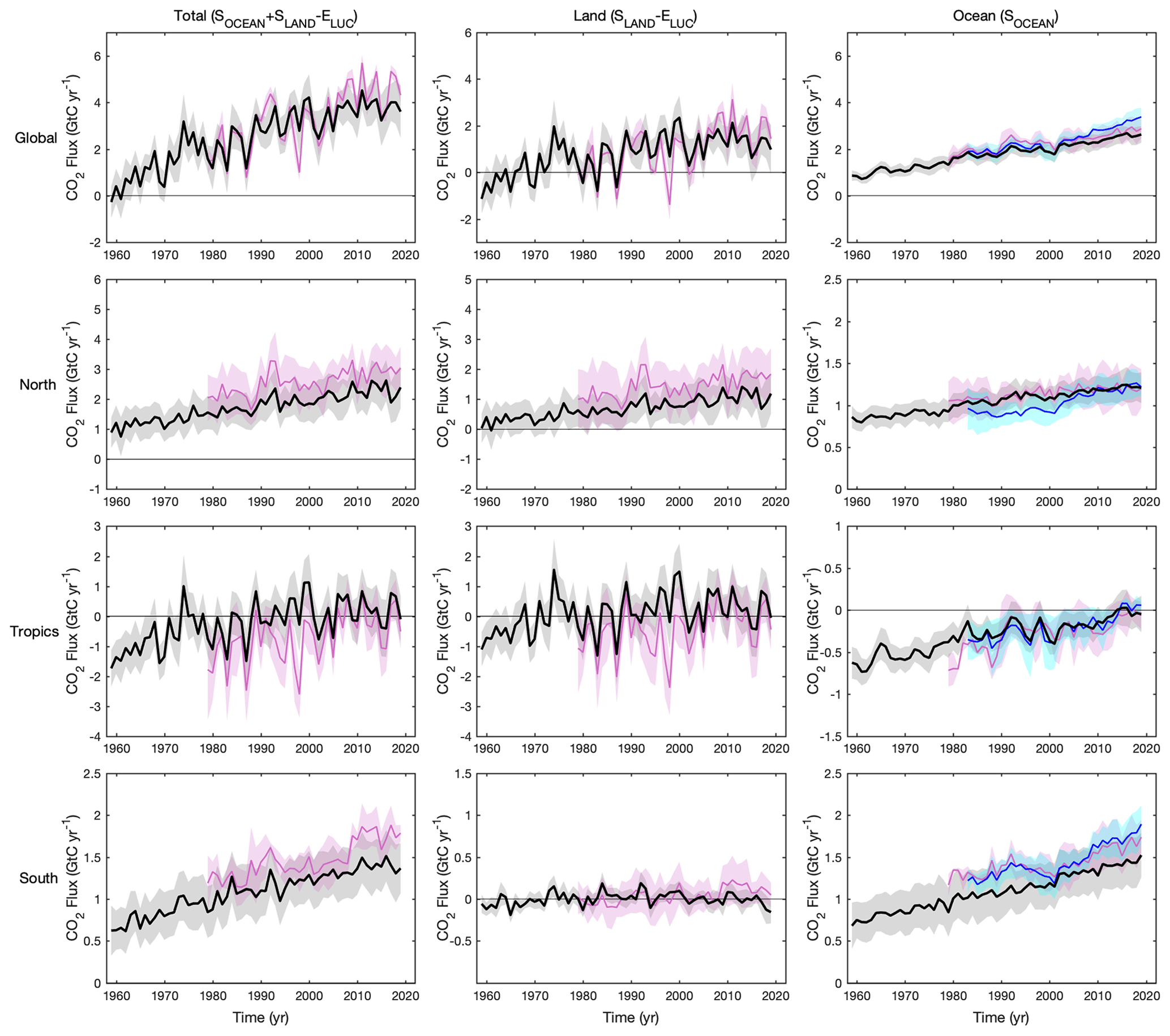
Figure 8CO2 fluxes between the atmosphere and the surface, SOCEAN and (SLAND – ELUC) by latitude bands for the (top row) globe, (second row) north (north of 30∘ N), (third row) tropics (30∘ S–30∘ N), and (bottom) south (south of 30∘ S), and over (left) total (), (middle) land only (SLAND−ELUC), and (right) ocean only (SOCEAN). Positive values indicate a flux from the atmosphere to the land and/or ocean. Mean estimates from the combination of the process models for the land and oceans are shown (black line) with ±1σ of the model ensemble (grey shading). For total uncertainty, the land and ocean uncertainties are summed in quadrature. Mean estimates from the atmospheric inversions are shown (pink lines) with their ±1σ spread (pink shading). Mean estimates from the pCO2-based flux products are shown for the ocean domain (dark blue lines) with their ±1σ spread (light blue shading). The global SOCEAN (upper right) and the sum of SOCEAN in all three regions represents the anthropogenic atmosphere-to-ocean flux based on the assumption that the pre-industrial ocean sink was 0 GtC yr−1 when riverine fluxes are not considered. This assumption does not hold on the regional level, where pre-industrial fluxes can be significantly different from zero. Hence, the regional panels for SOCEAN represent a combination of natural and anthropogenic fluxes. Bias-correction and area-weighting were only applied to global SOCEAN; hence the sum of the regions is slightly different from the global estimate (< 0.08 GtC yr−1).
3.2 Global carbon budget for the last decade (2010–2019)
The global carbon budget averaged over the last decade (2010–2019) is shown in Figs. 2 and 9 (right panel). For this time period, 86 % of the total emissions (EFOS+ELUC) were from fossil CO2 emissions (EFOS), and 14 % from land-use change (ELUC). The total emissions were partitioned among the atmosphere (46 %), ocean (23 %), and land (31 %), with an unattributed budget imbalance (−1 %).
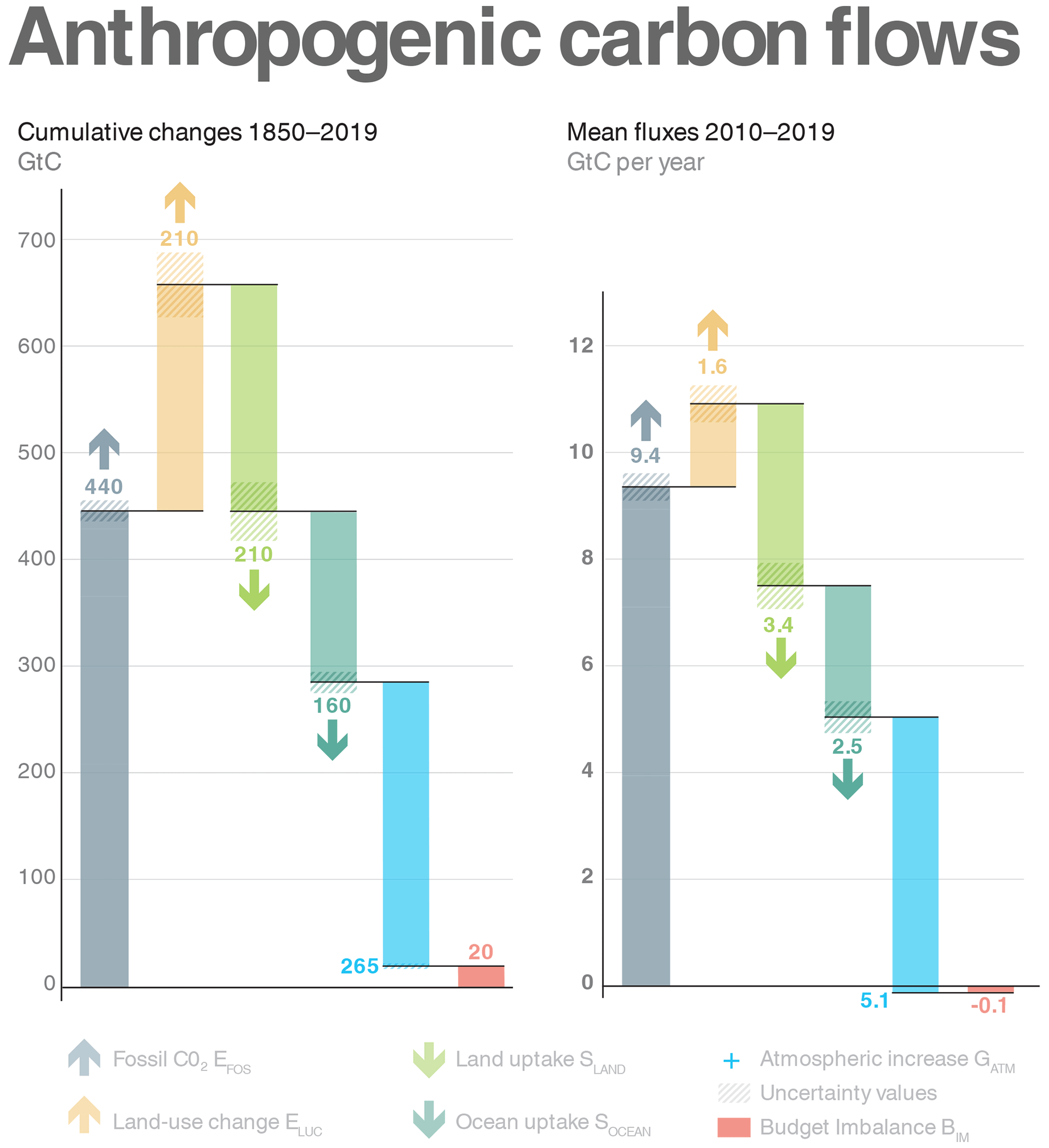
Figure 9Cumulative changes during 1850–2019 and mean fluxes during 2010–2019 for the anthropogenic perturbation as defined in the legend. Cement carbonation sink is included in EFOS.
3.2.1 CO2 emissions
Global fossil CO2 emissions grew at a rate of 1.2 % yr−1 for the last decade (2010–2019), with a decadal average of 9.6 ± 0.5 GtC yr−1 excluding the cement carbonation sink (9.4 ± 0.5 GtC yr−1 when the cement carbonation sink is included) (Fig. 5, Table 6). China's emissions increased by +1.2 % yr−1 on average (increasing by +0.046 GtC yr−1 during the 10-year period), dominating the global trend, followed by India's emissions increase by +5.1 % yr−1 (increasing by +0.025 GtC yr−1), while emissions decreased in EU27 by −1.4 % yr−1 (decreasing by −0.014 GtC yr−1) and in the USA by −0.7 % yr−1 (decreasing by −0.01 GtC yr−1). In the past decade, fossil CO2 emissions decreased significantly (at the 95 % level) in 24 growing economies: Barbados, Belgium, Croatia, Czech Republic, Denmark, Finland, France, Germany, Israel, Italy, Japan, Luxembourg, Malta, Mexico, the Netherlands, Norway, Romania, Slovakia, Slovenia, the Solomon Islands, Sweden, Switzerland, the United Kingdom, and the USA. The drivers of recent decarbonization are examined in Le Quéré et al. (2019).
In contrast, there is no clear trend in CO2 emissions from land-use change over the last decade (Fig. 6, Table 6), though the data are very uncertain, with partly diverging trends over the last decade (Sect. 3.1.1). Larger emissions are expected increasingly over time for DGVM-based estimates as they include the loss of additional sink capacity, while the bookkeeping estimates do not. The LUH2-GCB2020 data set also features large dynamics in land use in particular in the tropics in recent years, causing higher emissions in DGVMs, BLUE, and the OSCAR best-guess, which includes simulations based on LUH2-GCB2020, than in HandN2017.
3.2.2 Partitioning among the atmosphere, ocean, and land
The growth rate in atmospheric CO2 concentration increased during 2010–2019, with a decadal average of 5.1 ± 0.02 GtC yr−1, albeit with large interannual variability (Fig. 4). Averaged over that decade, the ocean and land sinks amount to 2.5 ± 0.6 GtC yr−1 and 3.4 ± 0.9 GtC yr−1 respectively. During 2010–2017, the ocean CO2 sink appears to have intensified in line with the expected increase from atmospheric CO2 (McKinley et al., 2020). This effect is stronger in the pCO2-based flux products (Fig. 7, McKinley et al., 2020). The reduction of −0.16 GtC yr−1 (range: −0.43 to +0.03 GtC yr−1) in the ocean CO2 sink in 2017 is consistent with the return to normal conditions after the El Niño in 2015–2016, which caused an enhanced sink in previous years.
The budget imbalance (Table 6) and the residual sink from global budget (Table 5) include an error term due to the inconsistency that arises from using ELUC from bookkeeping models, and SLAND from DGVMs. This error term includes the fundamental differences between bookkeeping models and DGVMs, most notably the loss of additional sink capacity. Other differences include an incomplete accounting of LUC practices and processes in DGVMs, while they are all accounted for in bookkeeping models by using observed carbon densities, and bookkeeping error of keeping present-day carbon densities fixed in the past. That the budget imbalance shows no clear trend towards larger values over time is an indication that the loss of additional sink capacity plays a minor role compared to other errors in SLAND or SOCEAN (discussed in Sect. 3.1.4).
3.2.3 Inter-comparison of flux estimates
Regionality
Figure 8 shows the partitioning of the total atmosphere-to-surface fluxes excluding fossil CO2 emissions () according to the multi-model average estimates from process models (GOBMs and DGVMs), atmospheric inversions and ocean pCO2-based products. Figure 8 provides information on the regional distribution of those fluxes by latitude bands. The global mean total atmosphere-to-surface CO2 flux from process models for 2010–2019 is 3.8 ± 0.7 GtC yr−1, below the global mean atmosphere-to-surface flux of 4.3 ± 0.5 GtC yr−1 inferred by the carbon budget (EFOS – GATM in Eq. 1; Table 6). The total atmosphere-to-surface CO2 flux from the inversions (4.5 ± 0.1 GtC yr−1) almost matches the value inferred by the carbon budget, which is expected due to the constraint on GATM incorporated within the inversion approach and the adjustment of the fossil emissions prior to a value consistent with the EFOS budget term (Jones et al., 2020; see Sect. 2.6).
In the southern extra-tropics (south of 30∘ S), the atmospheric inversions suggest a total atmosphere-to-surface sink () for 2010–2019 of 1.4 ± 0.3 GtC yr−1, similar to the process models' estimate of 1.4 ± 0.3 GtC yr−1 (Fig. 8). An approximately neutral total land flux (SLAND−ELUC) for the southern extra-tropics is estimated by both the DGVMs (0.0 ± 0.1 GtC yr−1) and the inversion models (sink of 0.1 ± 0.2 GtC yr−1). The GOBMs (1.4 ± 0.3 GtC yr−1) produce a lower estimate for the ocean sink than the inversion models (1.6 ± 0.2 GtC yr−1) or pCO2-based flux products (1.7 ± 0.1 GtC yr−1; discussed further below).
In the tropics (30∘ S–30∘ N), both the atmospheric inversions and process models suggest that the total carbon balance in this region () is close to neutral over the past decade. The inversion models indicate a small tropical source to the atmosphere of −0.2 ± 0.6 GtC yr−1, whereas the process models indicate a small sink of 0.2 ± 0.7 GtC yr−1. The GOBMs (−0.1 ± 0.2 GtC yr−1 source), inversion models (−0.1 ± 0.2 GtC yr−1 source), and pCO2-based flux products (−0.05 ± 0.02 GtC yr−1 source) all indicate an approximately neutral tropical ocean flux, meaning that the difference in sign of the total fluxes stems from the land component. Indeed, the DGVMs indicate a total land sink (SLAND−ELUC) of 0.2 ± 0.7 GtC yr−1, whereas the inversion models indicate a small land source of −0.1 ± 0.7 GtC yr−1, though with high uncertainty in both cases. Overall, the GOBMs, pCO2-based flux products, and inversion models suggest either a neutral ocean flux or a small ocean source, while the DGVMs and inversion models suggest either a small sink or source on land. The agreement between inversions and process models is significantly better for the last decade than for any previous decade (Fig. 8), although the reasons for this better agreement are still unclear.
In the northern extra-tropics (north of 30∘ N) the atmospheric inversions suggest an atmosphere-to-surface sink () for 2010–2019 of 2.9 ± 0.6 GtC yr−1, which is higher than the process models' estimate of 2.3 ± 0.6 GtC yr−1 (Fig. 8). The difference derives from the total land flux (SLAND−ELUC) estimate, which is 1.1 ± 0.6 GtC yr−1 in the DGVMs compared with 1.7 ± 0.8 GtC yr−1 in the inversion models. The GOBMs (1.2 ± 0.2 GtC yr−1), inversion models (1.2 ± 0.2 GtC yr−1) and pCO2-based flux products (1.2 ± 0.2 GtC yr−1) produce consistent estimates of the ocean sink.
The noteworthy differences between the annual estimates produced by different data sources are as follows:
- i.
The southern SOCEAN flux in the pCO2-based flux products and inversion models is higher than in the GOBMs. This might be explained by the data products potentially underestimating the winter CO2 outgassing south of the polar front (Bushinsky et al., 2019), or by the uncertainty in the regional distribution of the river flux adjustment (Aumont et al., 2001, Lacroix et al., 2020) applied to pCO2-based flux products to isolate the anthropogenic SOCEAN flux.
- ii.
The magnitude of the northern net land flux (SLAND−ELUC) is larger in inversion models than in the DGVMs. Discrepancies in the northern and tropical land fluxes conform with persistent issues surrounding the quantification of the drivers of the global net land CO2 flux (Arneth et al., 2017; Huntzinger et al., 2017) and the distribution of atmosphere-to-land fluxes between the tropics and high northern latitudes (Baccini et al., 2017; Schimel et al., 2015; Stephens et al., 2007; Ciais et al., 2019). These differences cannot be simply explained. They could either reflect a bias in the inversions or missing processes or biases in the process models, such as the lack of adequate parameterizations for land management for the DGVMs. In fact, the six inversions shown in Fig. 8 form two categories, one with a large northern land sink and a tropical land source and another with a moderate northern land sink and a small tropical sink (Sect. “Atmospheric inversion models differences”). The estimated contribution of the north and its uncertainty from process models is sensitive both to the ensemble of process models used, e.g. the inclusion of northern forest management in DGVMs and possibly emissions that are too strong from LUC (Bastos et al., 2020), and to the specifics of each inversion, e.g. zonal and latitudinal transport and its covariance with seasonal fluxes (Denning et al., 1995).
Interannual variability
The interannual variability in the southern extra-tropics is low because of the dominance of ocean area with low variability compared to land areas. The split between land (SLAND−ELUC) and ocean (SOCEAN) shows a small contribution to variability in the south coming from the land, with no consistency between the DGVMs and the inversions or among inversions. This is expected due to the difficulty of separating exactly the land and oceanic fluxes when viewed from atmospheric observations alone. The interannual variability, calculated as the standard deviation from detrended time series around the mean, was found to be similar in the pCO2-based flux products including Watson et al. (2020) (0.05 to 0.10 GtC yr−1) and GOBMs (0.06 to 0.17 GtC yr−1) in 2010–2019 (Fig. B1).
Both the process models and the inversions consistently allocate more year-to-year variability of CO2 fluxes to the tropics compared to the northern extra-tropics (Fig. 8). The land is the origin of most of the tropical variability, consistently among the process models and inversions. The interannual variability in the tropics is similar among the ocean flux products (0.03 to 0.09 GtC yr−1) and the models (0.02 to 0.09 GtC yr−1; Sect. 3.1.3, Fig. B1). The inversions indicate that atmosphere-to-land CO2 fluxes are more variable than atmosphere-to-ocean CO2 fluxes in the tropics and produce slightly higher IAV than the ocean flux products or GOBMs. With a sparsity of tropical atmospheric measurements, an aliasing of the large land flux variations onto the tropical ocean fluxes in the inversions is one likely cause of this difference.
In the northern extra-tropics, the models, inversions, and pCO2-based flux products consistently suggest that most of the variability stems from the land (Fig. 8). Inversions, GOBMs, and pCO2-based flux products agree on the mean of SOCEAN, but with a higher interannual variability in the pCO2-based flux products (0.05 to 0.08 GtC yr−1) than in the GOBMs (0.04 to 0.10 GtC yr−1; Fig. B1).
Atmospheric inversion models differences
The expanded ensemble of atmospheric inversions (from N=3 to N=6) allows a more representative sample of model–model differences, e.g. in latitudinal transport and other inversion settings (Table A4). When assessed for their tropical or northern land+ocean fluxes we see a dipole arise, where three models estimate a northern extra-tropical sink close to 2.5 GtC yr−1, and the other three a sink of close to 3.5 GtC yr−1. The inversions resulting in a large northern sink also estimate a tropical source. Both groups of models perform equally well on the evaluation metric of the misfit of optimized CO2 from inversions against independent aircraft data in Fig. B3 though, and resolving this difference will require the consideration and inclusion of larger volumes of semi-continuous observations of concentrations, fluxes, and auxiliary variables collected from (tall) towers close to the surface CO2 exchange. Improvements in model resolution and atmospheric transport realism together with expansion of the observational record (also in the data-sparse boreal Eurasian area) may help anchor the mid-latitude NH fluxes per continent. In addition, new metrics could potentially differentiate between the more and less realistic realizations of the Northern Hemisphere land sink shown in Fig. 8.
In previous versions of this publication, another hypothesized explanation was that differences in the prior data set used by the inversion models, and related adjustments to posterior estimates, drove inter-model disparity. However, separate analysis has shown that the influence of the chosen prior land and ocean fluxes is minor compared to other aspects of each inversion, and the majority (5 of 6) of the inversion models presented in this update now use a consistent prior for fossil emissions (Jones et al., 2020; see Sect. 2.6).
Finally, in the 2020 effort, two inverse systems (UoE and CAMS) used column CO2 products derived from GoSAT and OCO-2, respectively. Their estimated fluxes and performance on the metrics evaluated in this work were similar to their counterparts driven by in situ and flask observations, and hence these solutions were not included separately (as noted by Chevallier et al., 2019). Nevertheless, this convergence of solutions is an important prerequisite for the use of longer remote sensing CO2 time series in the future and could help to further study differences driven by observational coverage and/or sparseness of the current network. Also, column-CO2 products are likely to be less sensitive to vertical transport differences between models, believed to be a remaining source of uncertainty (Basu et al., 2018).
3.2.4 Budget imbalance
The budget imbalance (BIM) was low, −0.1 GtC yr−1 on average over 2010–2019, although the BIM uncertainty is large (1.4 GtC yr−1 over the decade). Also, the BIM shows significant departure from zero on yearly timescales (Fig. 4), highlighting unresolved variability of the carbon cycle, likely in the land sink (SLAND), given its large year-to-year variability (Figs. 4e and 6b), while the decadal variability could originate from both the land and ocean sinks, given unresolved discussions on the strength of the ocean carbon sink (Bushinsky et al., 2019; Watson et al., 2020) and its decadal variability (DeVries et al., 2019).
Although the budget imbalance is near zero for the recent decades, it could be due to compensation of errors. We cannot exclude an overestimation of CO2 emissions, in particular from land-use change, given their large uncertainty, as has been suggested elsewhere (Piao et al., 2018), combined with an underestimate of the sinks. A larger SLAND would reconcile model results with inversion estimates for fluxes in the total land during the past decade (Fig. 8; Table 5). Likewise, a larger SOCEAN is also possible given the higher estimates from the data products (see Sect. 3.1.2, Figs. 7 and 8) and the recently suggested upward correction of the ocean carbon sink (Watson et al., 2020; Fig. 7). If data products with the Watson et al. (2020) adjustment were to be used instead of GOBMs to estimate SOCEAN, this would result in a BIM of the order of −1 GtC yr−1 indicating that a closure of the budget could only be achieved with either anthropogenic emissions being larger and/or the net land sink being smaller than estimated here.
More integrated use of observations in the Global Carbon Budget, either on their own or for further constraining model results, should help resolve some of the budget imbalance (Peters et al., 2017; Sect. 4).
3.3 Global carbon budget for year 2019
3.3.1 CO2 emissions
Preliminary estimates of global fossil CO2 emissions are for growth of only 0.1 % between 2018 and 2019 to remain at 9.7 ± 0.5 GtC in 2019 (Fig. 5), distributed among coal (39 %), oil (34 %), natural gas (21 %), cement (4 %), and others (1.5 %). Compared to the previous year, emissions from coal decreased by 1.8 %, while emissions from oil, natural gas, and cement increased by 0.8 %, 2.0 %, and 3.2 %, respectively. All growth rates presented are adjusted for the leap year, unless stated otherwise.
In 2019, the largest absolute contributions to global fossil CO2 emissions were from China (28 %), the USA (14 %), the EU (27 member states; 8 %), and India (7 %). These four regions account for 57 % of global CO2 emissions, while the rest of the world contributed 43 %, which includes aviation and marine bunker fuels (3.5 % of the total). Growth rates for these countries from 2018 to 2019 were +2.2 % (China), −2.6 % (USA), −4.5 % (EU27), and +1.0 % (India), with +1.8 % for the rest of the world. The per capita fossil CO2 emissions in 2019 were 1.3 tC per person per year for the globe and were 4.4 (USA), 1.9 (China), 1.8 (EU27), and 0.5 (India) tC per person per year for the four highest-emitting countries (Fig. 5).
The growth in emissions of 0.1 % in 2019 is within the range of the projected growth of 0.6 % (range of −0.2 % to 1.5 %) published in Friedlingstein et al. (2019) based on national emissions projections for China, the USA, the EU27, and India and projections of gross domestic product corrected for IFOS trends for the rest of the world. The growth in emissions in 2019 for China, the USA, EU27, India, and the rest of the world were all within their previously projected range (Table 7).
Table 7Comparison of the projection with realized fossil CO2 emissions (excluding cement carbonation sink). The “actual” values are first the estimate available using actual data, and the “projected” values refer to estimates made before the end of the year for each publication. Projections based on a different method from that described here during 2008–2014 are available in Le Quéré et al. (2016). All values are adjusted for leap years.
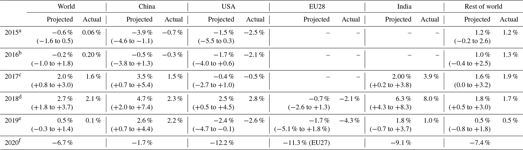
a Jackson et al. (2016) and Le Quéré et al. (2015a). b Le Quéré et al. (2016). c Le Quéré et al. (2018a). d Le Quéré et al. (2018b). e Friedlingstein et al. (2019). f This study (median of four reported estimates, Sect. “2020 projections”).
The largest absolute contributions to global CO2 emissions from a consumption perspective were China (25 %), the USA (16 %), the EU (10 %), and India (6 %) for 2016, the last year with available data. The difference between territorial and consumption emissions (the net emission transfer via international trade) has generally increased from 1990 to around 2005 and remained relatively stable afterwards until the last year available (2016; Fig. 5).
The global CO2 emissions from land-use change are estimated to be 1.8 ± 0.7 GtC in 2019, slightly larger than the previous decade, which results in particular from the high peat and tropical deforestation/degradation fires. First, unusually dry conditions for a non-El Niño year occurred in Indonesia in 2019, which led to fire emissions from peat burning, deforestation, and degradation in equatorial Asia to be about twice as large as the average over the previous decade (GFED4.1s, van der Werf et al., 2017). Second, 2019 saw a surge in deforestation fires in the Amazon, causing about 30 % higher emissions from deforestation and degradation fires over the previous decade (GFED4.1s, van der Werf et al., 2017). This development was evident also in deforestation rates, where 2019 (August 2018–July 2019), with 10.1 km2 forest clear-cut, saw the highest rate since 2008 (INPE, 2020). However, confidence in the annual change remains low. This brings the total CO2 emissions from fossil plus land-use change (EFOS+ELUC) to 11.5 ± 0.9 GtC (42.2 ± 3.3 GtCO2).
3.3.2 Partitioning among the atmosphere, ocean, and land
The growth rate in atmospheric CO2 concentration corresponded to 5.4 ± 0.2 GtC in 2019 (2.54 ± 0.08 ppm; Fig. 4; Dlugokencky and Tans, 2020), slightly above the 2010–2019 average of 5.1 ± 0.02 GtC yr−1.
The estimated ocean CO2 sink was 2.6 ± 0.6 GtC in 2019. Although there is a significant difference of SOCEAN between GOBMs (2.6 GtC) and pCO2-based products (3.4 GtC), they both suggest an average increase of 0.06–0.07 GtC in 2019 compared to 2018. Six models and two flux products show an increase in SOCEAN (GOBM up to +0.30 GtC, data product up to +0.29 GtC), while three models and two flux products show no change or a decrease in SOCEAN (GOBMs down to −0.03 GtC, data products down to −0.17 GtC; Fig. 7).
The terrestrial CO2 sink from the DGVM model ensemble was 3.1 ± 1.2 GtC in 2019, slightly below the decadal average (Fig. 4) and consistent with constraints from the rest of the budget (Table 5). Atmospheric inversions confirm a lower-than-average land sink in 2019 and consistently estimate this as an increased source from the tropical land (+0.3 GtC). The budget imbalance was +0.3 GtC in 2019, which is above the average over the last decade (Table 6). This imbalance is indicative only, given its significant year-to-year variability and large uncertainty (1.4 GtC yr−1).
3.4 Global carbon budget projection for year 2020
3.4.1 Fossil CO2 emissions
We present the results from the four separate methods in Table A8, with monthly results for each country, for each region, and globally shown in Fig. B5. The restrictions implemented in response to COVID-19 led to dramatic and unprecedented changes in society, and this caused large changes in CO2 emissions. All countries had significant deviations from their previous emission trends.
Year to date (YTD)
The four methods presented here use a mix of direct emissions estimates from energy consumption data to the use of proxies as indicators of changes in activity levels. Annual historical CO2 emissions estimates (pre-2020) are largely derived from reported energy data. For 2020, we do not have sufficient information to say that the use of monthly energy data gives any more accurate estimates than proxy approaches. Monthly energy consumption data are subject to revisions and can be estimated or incomplete, and it is not known if proxy data may perform better. A full evaluation of monthly and proxy methods can only be made when full-year data become available. As noted in Forster et al. (2020) the reductions in CO2 emissions may be about 20 % overestimated based on meteorologically adjusted NOx observations.
The YTD results (Fig. B5, Table A8) run to September for all regions and methods, except the EU27 which is to July (limited by the Eurostat data used by the GCB method). To September (July) 2020, the four methods indicate fossil CO2 emissions were down in all regions and globally. However, the background for these declines varies by country. The EU and the USA had declining emission trends before COVID-19, so the pandemic effect is on top of these existing emission reductions. In both the EU and the USA, reductions in coal use have been accelerated by COVID-19. Similarly, India's emissions were in decline through 2019, but this time because of economic troubles (Andrew, 2020b), but COVID-19 is potentially superimposed on the longer-term trend of increasing emissions in India. In contrast, China and the rest of the world have the COVID-19 effect on the top of rising emissions. China has lower reductions, but this may also indicate that the full impact of the COVID-19 restrictions occurred earlier and the economy has had a longer time to recover.
Based on the three studies providing sufficient data, from January to September, global emissions may have declined by around 8 % (median, based on model estimates of −7.6 %, UEA; −7.6 %, Carbon Monitor; −14.1 %, Priestley Centre). This range between estimates does not include the uncertainty inherent in each method, which would increase the spread.
2020 projections
The full-year projection for 2020 must necessarily be interpreted cautiously. Only Le Quéré et al. (2020) include a formal projection, by assuming confinement measures in place on 13 November remain in place until the end of the year at current or lower levels in each country. Forster et al. (2020) use a simple extrapolation, assuming the declines in emissions from their baselines remain at 66 % of the level over the last 30 d with estimates. Liu et al. (2020) and the GCB method did not perform a projection for 2020, and for purposes of comparison we use a simple approach to extrapolating their observations by assuming the remaining months of the year change by the same relative amount compared to 2019 as the final month of observations.
Based on these assumptions, the countries and regions considered are all expected to see a decline in annual total emissions, with the potential exception of China, which may have a slight increase according to Carbon Monitor and the GCB method (Fig. B5). The year 2020 is behaving in many ways entirely differently to any year in history, and the confidence in the 2020 projection is therefore currently low, due to both the spread in results and the uncertain developments of the disease itself, strength of future societal and industrial restrictions, and stimulus packages throughout the remainder of 2020. The largest source of uncertainty comes from the emissions in China, because of the limited available information both on monthly emissions and for proxy data, and emissions for the rest of the world, because it represents around 40 % of the world's emissions in aggregate.
Based on the median value of the four methods considered, global emissions may decline by about 7 % in 2020 (−5.8 %, GCB; −6.5 %, Carbon Monitor; −6.9 % (range −2.7 to −10.8 %), UEA; −13.0 %, Priestley Centre), with additional uncertainty from each method on top of this (Fig. B5, Table A8). Using a purely GDP-based projection, based on the IMF GDP forecast as of June 2020, and assuming the 10-year trend in CO2∕GDP continues in 2020, emissions would decline by 7.5 % – well within the range of other estimates. In October 2020, the IEA forecasted a drop of 7 % in fossil energy emissions (IEA, 2020). The decrease in emissions for the full year 2020 appears more pronounced in the USA, EU27, and India, partly due to pre-existing trends. In contrast the decrease in emissions appears to be least pronounced in China, where restriction measures associated with COVID-19 occurred early in the year and lockdown measures were more limited in time.
Synthesis
Given a negative median growth rate of about −7 % across methods, global fossil CO2 emissions (EFOS) would be around 9.0 GtC (33.2 GtCO2) in 2020, assuming a cement carbonation sink of 0.2 GtC yr−1 (Table A8). These figures do not include the uncertainty from this method in projecting 2020 emissions.
Our preliminary estimates of fire emissions in deforestation zones and Amazon deforestation rates indicate that emissions from land-use change (ELUC) for 2020 are similar to the 2010–2019 average (Sect. 2.2.4). We therefore expect ELUC emissions of around 1.6 GtC in 2020. The apparent decrease in the mean value of ELUC emissions compared to 2019 is largely related to the transition from an anomalously dry to a wet year in Indonesia (see Sects. 2.2.4 and 3.2.1 for detail).
We hence project global total anthropogenic CO2 emissions from fossil and land-use changes to be around 10.6 GtC (39 GtCO2) in 2020.
3.4.2 Partitioning among the atmosphere, ocean, and land
The 2020 growth in atmospheric CO2 concentration (GATM) is projected to be about 5.3 GtC (2.5 ppm) based on GLO observations until the end of August 2020, bringing the atmospheric CO2 concentration to an expected level of 412 ppm averaged over the year. Combining projected EFOS, ELUC and GATM suggests a combined land and ocean sink (SLAND+SOCEAN) of about 5.3 GtC for 2020. Although each term has large uncertainty, the oceanic sink SOCEAN has generally low interannual variability and is likely to remain close to its 2019 value of around 2.6 GtC, leaving a rough estimated land sink SLAND (including any budget imbalance) of around 2.7 GtC, slightly below the 2019 estimate.
3.5 Cumulative sources and sinks
Cumulative historical sources and sinks are estimated as in Eq. (1) with semi-independent estimates for each term and a global carbon budget imbalance. Cumulative fossil CO2 emissions for 1850–2019 were 445 ± 20 GtC for EFOS and 210 ± 60 GtC for ELUC (Table 8; Fig. 9), for a total of 650 ± 65 GtC. The cumulative emissions from ELUC are particularly uncertain, with large spread among individual estimates of 150 GtC (HandN2017), 275 GtC (BLUE), and 200 GtC (OSCAR) for the three bookkeeping models and a similar wide estimate of 200 ± 60 GtC for the DGVMs. These estimates are consistent with indirect constraints from vegetation biomass observations (Li et al., 2017), but given the large spread a best estimate is difficult to ascertain.
Table 8Cumulative CO2 for different time periods in gigatonnes of carbon (GtC). All uncertainties are reported as ±1σ. The budget imbalance provides a measure of the discrepancies among the nearly independent estimates. Its uncertainty exceeds ±60 GtC. The method used here does not capture the loss of additional sink capacity from reduced forest cover, which is about 20 GtC and would exacerbate the budget imbalance (see Sect. 2.7.4). All values are rounded to the nearest 5 GtC and therefore columns do not necessarily add to zero. Cement carbonation sink is included in EFOS.

a Using projections for the year 2020 (Sect. 3.4). Uncertainties are the same as the 1850–2019 period. b Cumulative ELUC 1750–1849 of 30 GtC based on multi-model mean of Pongratz et al. (2009), Shevliakova et al. (2009), Zaehle et al. (2011), and Van Minnen et al. (2009). 1850–2019 from mean of HandN2017 (Houghton and Nassikas, 2017) and BLUE (Hansis et al., 2015). 1750–2019 uncertainty is estimated from standard deviation of DGVMs over 1870–2019 scaled by 1750–2019 emissions. c Cumulative ELUC based on HandN, BLUE, and OSCAR. Uncertainty is estimated from the standard deviation of DGVM estimates. d Cumulative ELUC based on HandN, BLUE, and OSCAR. Uncertainty is formed from the uncertainty in annual ELUC over 1959–2019, which is 0.7 GtC yr−1 multiplied by length of the time series. e Ocean sink uncertainty from IPCC (Denman et al., 2007).
Emissions during the period 1850–2019 were partitioned among the atmosphere (265 ± 5 GtC; 40 %), ocean (160 ± 20 GtC; 25 %), and land (210 ± 55 GtC; 32 %). This cumulative land sink is broadly equal to the cumulative land-use emissions, making the global land nearly neutral over the 1850–2019 period. The use of nearly independent estimates for the individual terms shows a cumulative budget imbalance of 20 GtC (3 %) during 1850–2019 (Fig. 2), which, if correct, suggests that emissions are too high by the same proportion or that the land or ocean sinks are underestimated. The bulk of the imbalance could originate from the estimation of large ELUC between the mid-1920s and the mid-1960s, which is unmatched by a growth in atmospheric CO2 concentration as recorded in ice cores (Fig. 3). The known loss of an additional sink capacity of 30–40 GtC due to reduced forest cover has not been accounted for in our method and would further exacerbate the budget imbalance (Sect. 2.7.4).
Cumulative emissions through to the year 2020 increase to 655 ± 65 GtC (2340 ± 240 GtCO2), with about 70 % contribution from EFOS and about 30 % contribution from ELUC. Cumulative emissions and their partitioning for different periods are provided in Table 8.
Given the large and persistent uncertainties in historical cumulative emissions, we suggest extreme caution is needed if using this estimate to determine the remaining cumulative CO2 emissions consistent with an ambition to stay below a given temperature limit (Millar et al., 2017; Rogelj et al., 2016, 2019).
Each year when the global carbon budget is published, each flux component is updated for all previous years to consider corrections that are the result of further scrutiny and verification of the underlying data in the primary input data sets. Annual estimates may be updated with improvements in data quality and timeliness (e.g. to eliminate the need for extrapolation of forcing data such as land use). Of all terms in the global budget, only the fossil CO2 emissions and the growth rate in atmospheric CO2 concentration are based primarily on empirical inputs supporting annual estimates in this carbon budget. The carbon budget imbalance, yet an imperfect measure, provides a strong indication of the limitations in observations in understanding and representing processes in models, and/or in the integration of the carbon budget components.
The persistent unexplained variability in the carbon budget imbalance limits our ability to verify reported emissions (Peters et al., 2017) and suggests we do not yet have a complete understanding of the underlying carbon cycle dynamics. Resolving most of this unexplained variability should be possible through different and complementary approaches. First, as intended with our annual updates, the imbalance as an error term is reduced by improvements of individual components of the global carbon budget that follow from improving the underlying data and statistics and by improving the models through the resolution of some of the key uncertainties detailed in Table 9. Second, additional clues to the origin and processes responsible for the variability in the budget imbalance could be obtained through a closer scrutiny of carbon variability in light of other Earth system data (e.g. heat balance, water balance), and the use of a wider range of biogeochemical observations to better understand the land–ocean partitioning of the carbon imbalance (e.g. oxygen, carbon isotopes). Finally, additional information could also be obtained through higher resolution and process knowledge at the regional level, and through the introduction of inferred fluxes such as those based on satellite CO2 retrievals. The limit of the resolution of the carbon budget imbalance is as yet unclear but most certainly not yet reached given the possibilities for improvements that lie ahead.
Table 9Major known sources of uncertainties in each component of the Global Carbon Budget, defined as input data or processes that have a demonstrated effect of at least ±0.3 GtC yr−1.

a As result of interactions between land use and climate. b The uncertainties in GATM have been estimated to be ±0.2 GtC yr−1, although the conversion of the growth rate into a global annual flux assuming instantaneous mixing throughout the atmosphere introduces additional errors that have not yet been quantified. c Could in part be due to uncertainties in atmospheric forcing (Swart et al., 2014).
Estimates of global fossil CO2 emissions from different data sets are in relatively good agreement when the different system boundaries of these data sets are taken into account (Andrew, 2020a). But while estimates of EFOS are derived from reported activity data requiring much less complex transformations than some other components of the budget, uncertainties remain, and one reason for the apparently low variation between data sets is precisely the reliance on the same underlying reported energy data. This year we have added cement carbonation, a carbon sink, to EFOS.The budget excludes some sources of fossil CO2 emissions, which available evidence suggests are relatively small (< 1 %). In non-Annex I countries, and before 1990 in Annex I countries, we still omit emissions from carbonate decomposition apart from those in cement production, a focus of future updates. We have also included new estimates for India, which are now for the calendar year instead of its fiscal year and include the significant changes in coal stocks missing from other data sets. Estimates for Japan and Australia, two other large emitters, are still reported for fiscal years not aligned with the calendar year. Some errors in pre-1950 emissions were uncovered by Andrew (2020a), and these have been corrected this year.
Estimates of ELUC suffer from a range of intertwined issues, including the poor quality of historical land-cover and land-use change maps, the rudimentary representation of management processes in most models, and the confusion in methodologies and boundary conditions used across methods (e.g. Arneth et al., 2017; Pongratz et al., 2014; see also Sect. 2.7.4 on the loss of sink capacity). Uncertainties in current and historical carbon stocks in soils and vegetation also add uncertainty in the LUC flux estimates. Unless a major effort to resolve these issues is made, little progress is expected in the resolution of ELUC. This is particularly concerning given the growing importance of ELUC for climate mitigation strategies, and the large issues in the quantification of the cumulative emissions over the historical period that arise from large uncertainties in ELUC.
The assessment of the GOBMs used for SOCEAN with flux products based on observations highlights a substantial discrepancy in the Southern Ocean (Fig. 8, Hauck et al., 2020). The long-standing sparse data coverage of pCO2 observations in the Southern compared to the Northern Hemisphere (e.g. Takahashi et al., 2009) continues to exist (Bakker et al., 2016, 2020) and to lead to substantially higher uncertainty in the SOCEAN estimate for the Southern Hemisphere (Watson et al., 2020). This discrepancy points to the need for increased high-quality pCO2 observations, especially in the Southern Ocean. Further uncertainty stems from the regional distribution of the river flux adjustment term being based on one model study yielding the largest riverine outgassing flux south of 20∘ S (Aumont et al., 2001), with a recent study questioning this distribution (Lacroix et al., 2020). The data products suggest an underestimation of variability in the GOBMs globally and, consequently, the variability in SOCEAN appears to be underestimated. The size of the underestimation of the amplitude of interannual variability (order of < 0.1 GtC yr−1, A-IAV; see Fig. B1) could account for some of the budget imbalance, but not all of it.
The assessment of the net land–atmosphere exchange derived from land sinks and net land-use change flux with atmospheric inversions also shows a substantial discrepancy, particularly for the estimate of the total land flux over the northern extra-tropics in the past decade. This discrepancy highlights the difficulty to quantify complex processes (CO2 fertilization, nitrogen deposition, N fertilizers, climate change and variability, land management, etc.) that collectively determine the net land CO2 flux. Resolving the differences in the Northern Hemisphere land sink will require the consideration and inclusion of larger volumes of observations (Sect. 3.2.3).
As introduced in 2018, we provide metrics for the evaluation of the ocean and land models and the atmospheric inversions. These metrics expand the use of observations in the global carbon budget, helping (1) to support improvements in the ocean and land carbon models that produce the sink estimates, and (2) to constrain the representation of key underlying processes in the models and to allocate the regional partitioning of the CO2 fluxes. However, GOBMs have changed little since the introduction of the ocean model evaluation. This is an initial step towards the introduction of a broader range of observations that we hope will support continued improvements in the annual estimates of the global carbon budget.
We assessed before that a sustained decrease of −1 % in global emissions could be detected at the 66 % likelihood level after a decade only (Peters et al., 2017). Similarly, a change in behaviour of the land and/or ocean carbon sink would take as long to detect, and much longer if it emerges more slowly. To continue reducing the carbon imbalance on annual to decadal timescales, regionalizing the carbon budget and integrating multiple variables are powerful ways to shorten the detection limit and ensure the research community can rapidly identify issues of concern in the evolution of the global carbon cycle under the current rapid and unprecedented changing environmental conditions.
The estimation of global CO2 emissions and sinks is a major effort by the carbon cycle research community that requires a careful compilation and synthesis of measurements, statistical estimates, and model results. The delivery of an annual carbon budget serves two purposes. First, there is a large demand for up-to-date information on the state of the anthropogenic perturbation of the climate system and its underpinning causes. A broad stakeholder community relies on the data sets associated with the annual carbon budget including scientists, policy makers, businesses, journalists, and non-governmental organizations engaged in adapting to and mitigating human-driven climate change. Second, over the last decade we have seen unprecedented changes in the human and biophysical environments (e.g. changes in the growth of fossil fuel emissions, impact of the COVID-19 pandemic, Earth's warming, and strength of the carbon sinks), which call for frequent assessments of the state of the planet, a better quantification of the causes of changes in the contemporary global carbon cycle, and an improved capacity to anticipate its evolution in the future. Building this scientific understanding to meet the extraordinary climate mitigation challenge requires frequent, robust, transparent, and traceable data sets and methods that can be scrutinized and replicated. This paper helps to keep track of new budget updates via “living data”.
The data presented here are made available in the belief that their wide dissemination will lead to greater understanding and new scientific insights into how the carbon cycle works, how humans are altering it, and how we can mitigate the resulting human-driven climate change. The free availability of these data does not constitute permission for publication of the data. For research projects, if the data are essential to the work, or if an important result or conclusion depends on the data, co-authorship may need to be considered for the relevant data providers. Full contact details and information on how to cite the data shown here are given at the top of each page in the accompanying database and summarized in Table 2.
The accompanying database includes two Excel files organized in the following spreadsheets.
The file Global_Carbon_Budget_2020v1.0.xlsx includes the following:
-
summary;
-
the global carbon budget (1959–2019);
-
global CO2 emissions from fossil fuels and cement production by fuel type, and the per capita emissions (1959–2019);
-
CO2 emissions from land-use change from the individual methods and models (1959–2019);
-
ocean CO2 sink from the individual ocean models and pCO2-based products (1959–2019);
-
terrestrial CO2 sink from the DGVMs (1959–2019);
-
additional information on the historical global carbon budget prior to 1959 (1750–2019).
-
cement carbonation sink (1959–2019);
-
additional information on the historical global carbon budget prior to 1959 (1750–2019).
The file National_Carbon_Emissions_2020v1.0.xlsx includes the following:
-
summary;
-
territorial country CO2 emissions from fossil CO2 emissions (1959–2019) from CDIAC with UNFCCC data overwritten where available, extended to 2019 using BP data;
-
consumption country CO2 emissions from fossil CO2 emissions and emissions transfer from the international trade of goods and services (1990–2016) using CDIAC/UNFCCC data (worksheet 3 above) as reference;
-
emissions transfers (Consumption minus territorial emissions; 1990–2016);
-
country definitions;
-
details of disaggregated countries;
-
details of aggregated countries;
Both spreadsheets are published by the Integrated Carbon Observation System (ICOS) Carbon Portal and are available at https://doi.org/10.18160/gcp-2020 (Friedlingstein et al., 2020). National emissions data are also available from the Global Carbon Atlas (http://www.globalcarbonatlas.org/, last access: 16 November 2020).
Table A1Comparison of the processes included in the bookkeeping method and DGVMs in their estimates of ELUC and SLAND. See Table 4 for model references. All models include deforestation and forest regrowth after abandonment of agriculture (or from afforestation activities on agricultural land). Processes relevant for ELUC are only described for the DGVMs used with land-cover change in this study (Fig. 6a and b).

a Refers to the routine harvest of established managed forests rather than pools of harvested products.
b No back and forth transitions between vegetation types at the country level, but if forest loss based on FRA exceeded agricultural expansion based on FAO, then this amount of area was cleared for cropland and the same amount of area of old croplands abandoned.
c Limited. Nitrogen uptake is simulated as a function of soil C, and Vcmax is an empirical function of canopy N. Does not consider N deposition.
d Available but not active.
e Simple parameterization of nitrogen limitation based on Yin (2002; assessed on FACE experiments).
f Although C–N cycle interactions are not represented, the model includes a parameterization of down-regulation of photosynthesis as CO2 increases to emulate nutrient constraints (Arora et al., 2009).
g Tillage is represented over croplands by increased soil carbon decomposition rate and reduced humification of litter to soil carbon.
h ISBA-CTRIP corresponds to SURFEXv8 in GCB2018.
i Bookkeeping models include the effect of CO2 fertilization as captured by present-day carbon densities, but not as an effect transient in time.
j As far as the DGVMs that OSCAR is calibrated to include it.
k Perfect fertilization assumed; i.e. crops are not nitrogen limited and the implied fertilizer diagnosed.
l Fire intensity responds to climate and CO2, but no fire suppression.
m Process captured implicitly by use of observed carbon densities.
Table A2Comparison of the processes and model set-up for the global ocean biogeochemistry models for their estimates of SOCEAN. See Table 4 for model references.
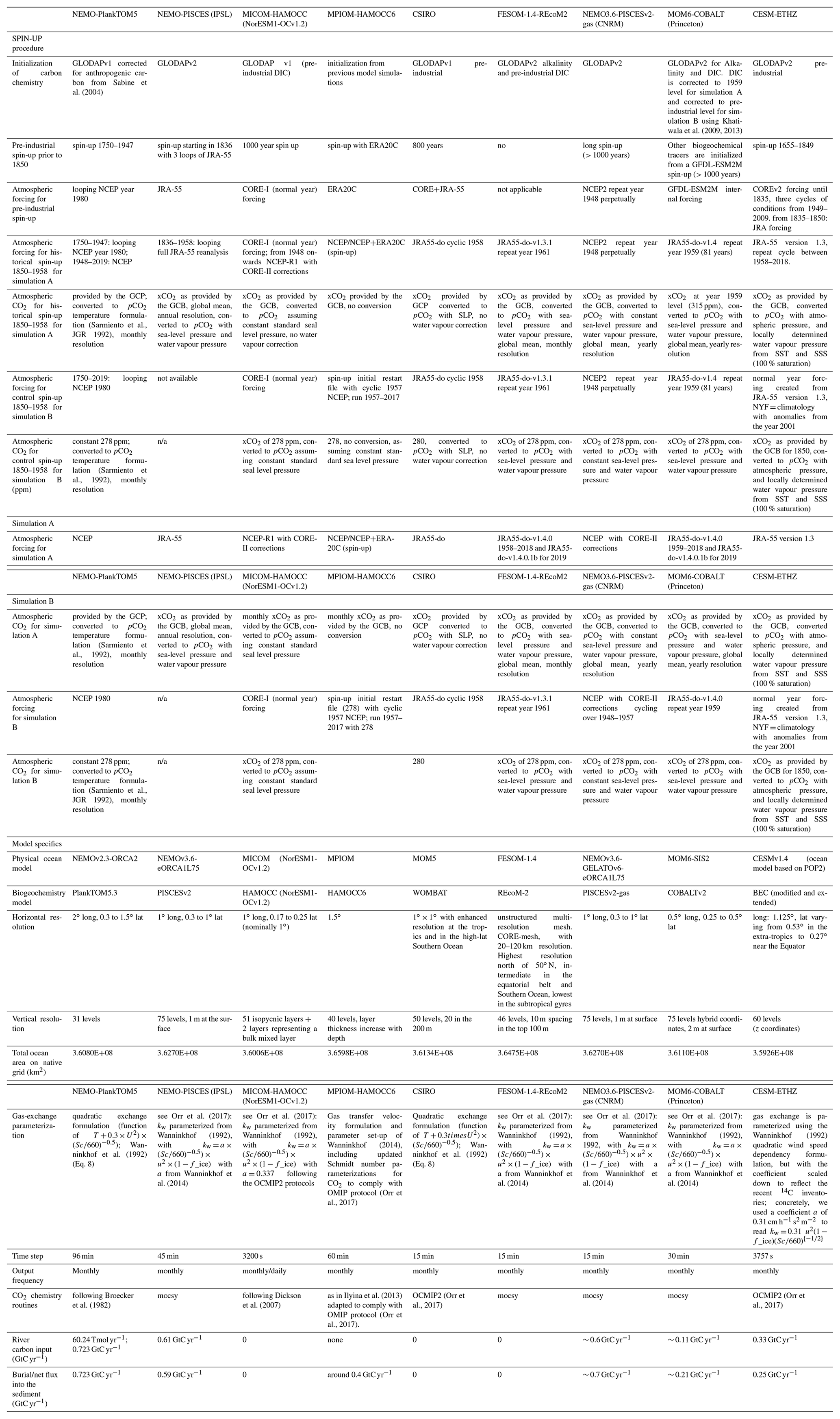
Table A3Description of ocean data products used for assessment of SOCEAN. See Table 4 for references.
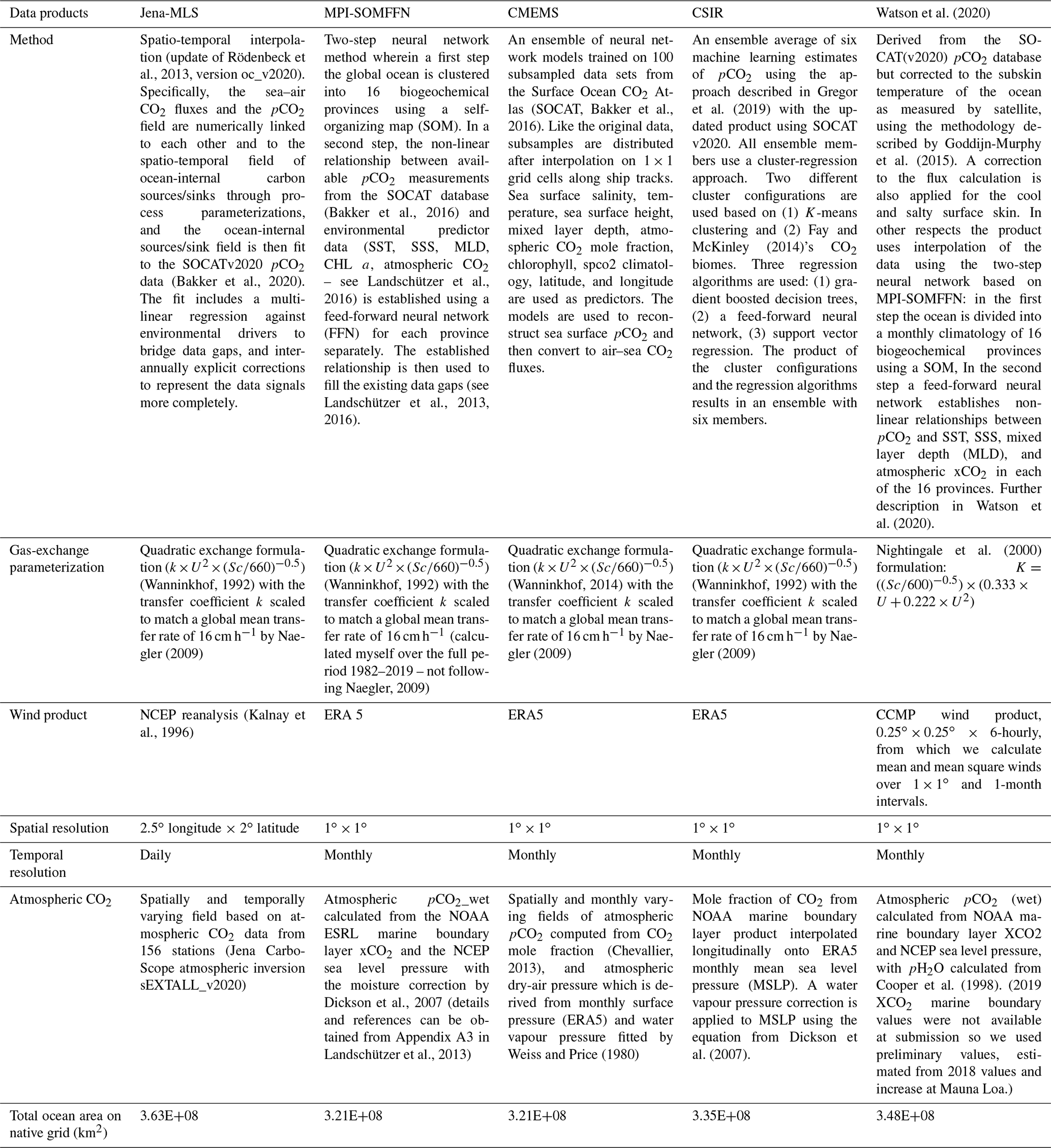
Table A4Comparison of the inversion set-up and input fields for the atmospheric inversions. Atmospheric inversions see the full CO2 fluxes, including the anthropogenic and pre-industrial fluxes. Hence they need to be adjusted for the pre-industrial flux of CO2 from the land to the ocean that is part of the natural carbon cycle before they can be compared with SOCEAN and SLAND from process models. See Table 4 for references.
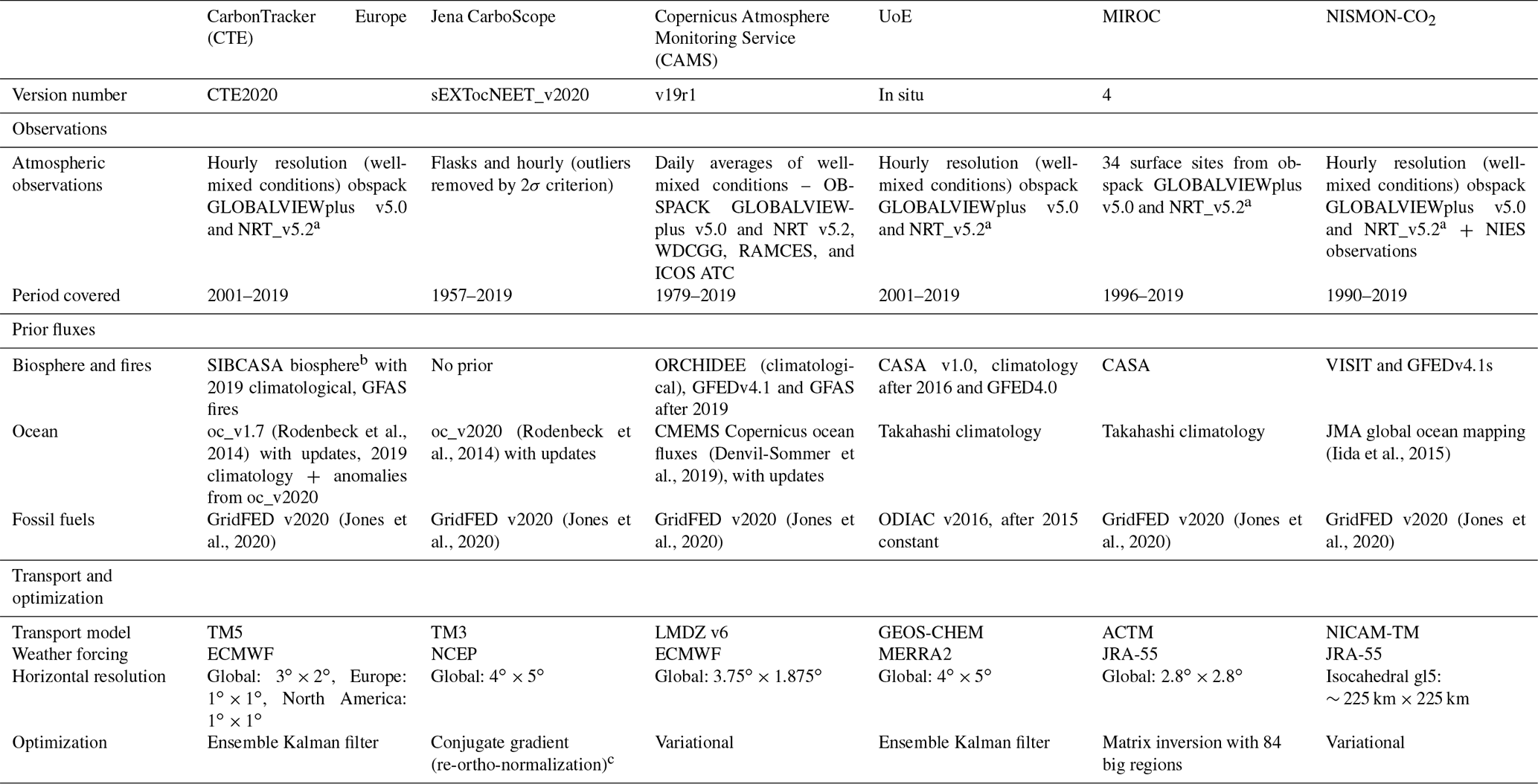
a CGADIP (2020), Carbontracker Team (2020), b van der Velde et al. (2014), c ocean prior not optimized.
Table A5Attribution of fCO2 measurements for the year 2019 included in SOCATv2020 (Bakker et al., 2016, 2020) to inform ocean pCO2-based flux products.
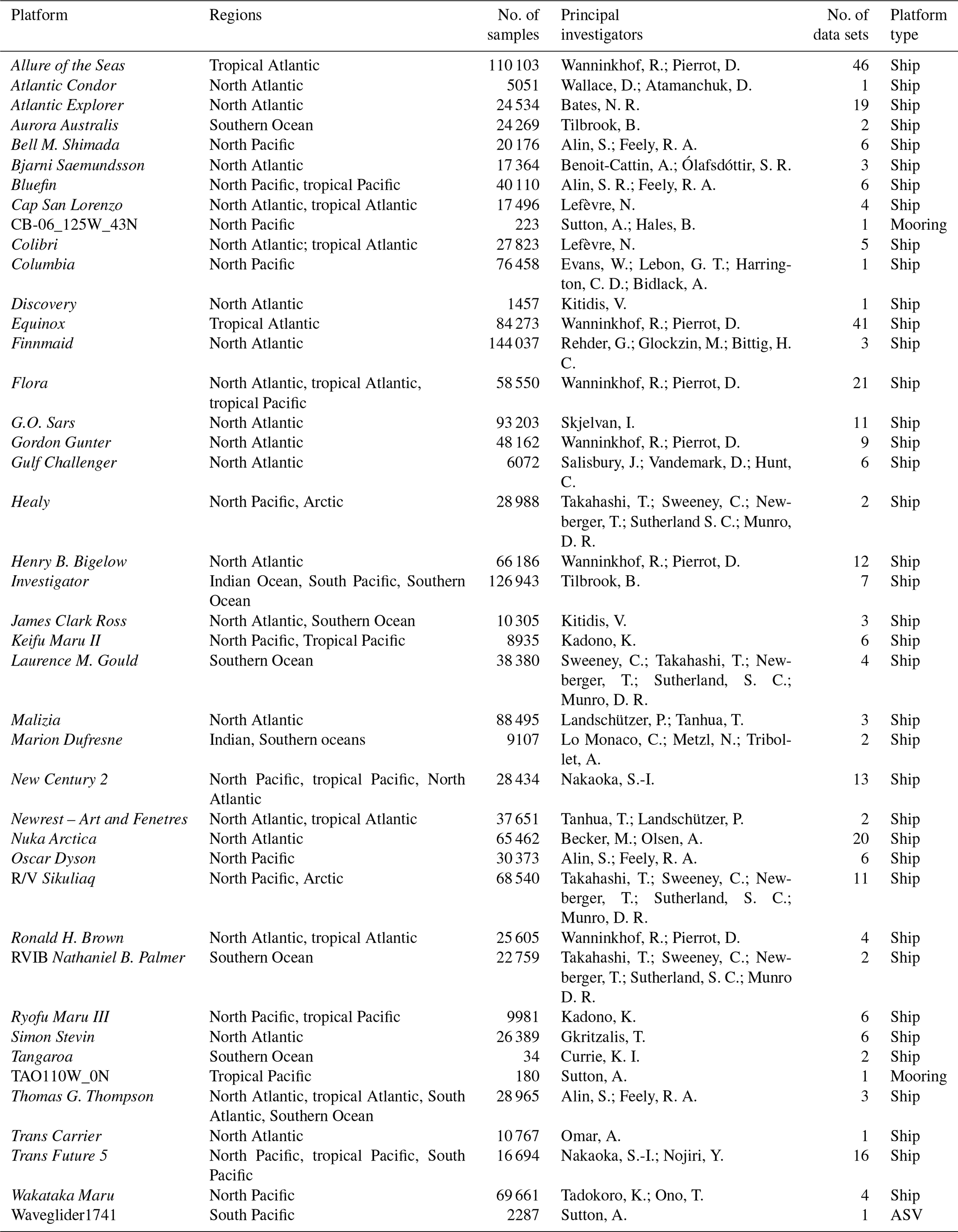
Table A6Aircraft measurement programs archived by Cooperative Global Atmospheric Data Integration Project (CGADIP, 2020) that contribute to the evaluation of the atmospheric inversions (Fig. B3).

Table A7Main methodological changes in the global carbon budget since first publication. Methodological changes introduced in one year are kept for the following years unless noted. Empty cells mean there were no methodological changes introduced that year.
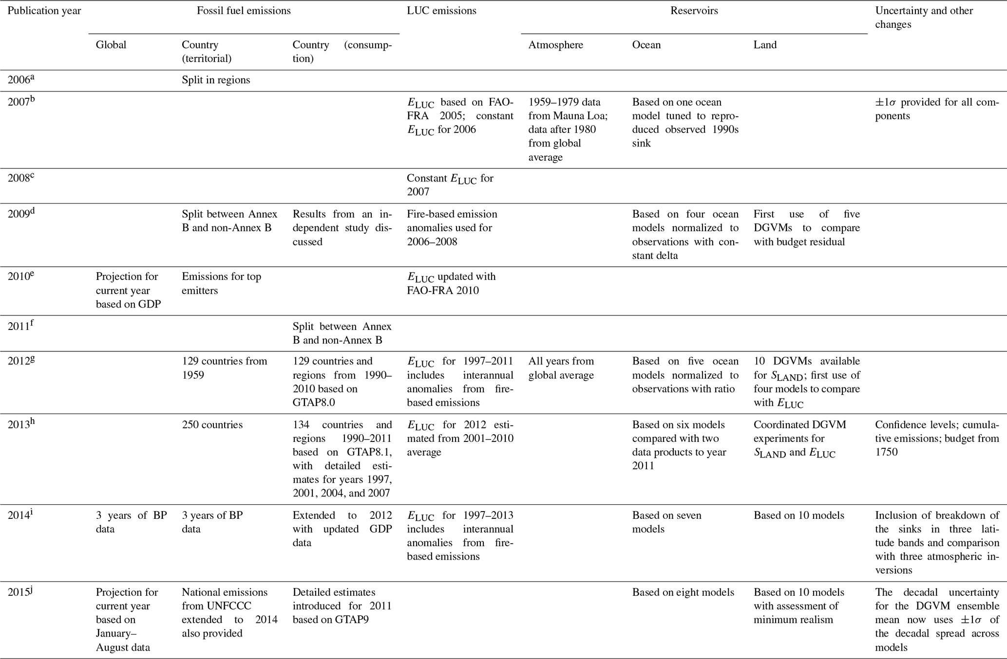
a Raupach et al. (2007), b Canadell et al. (2007), c Online, d Le Quéré et al. (2009), e Friedlingstein et al. (2010), f Peters et al. (2012b), g Le Quéré et al. (2013), Peters et al. (2013), h Le Quéré et al. (2014), i Le Quéré et al. (2015b), j Le Quéré et al. (2016).
Table A8Relative changes in fossil CO2 emissions (excluding cement carbonation sink) for the year 2020 to date and projections for the full year. Methods of the four approaches are described in Sect. 2.1.5 and Appendix C.
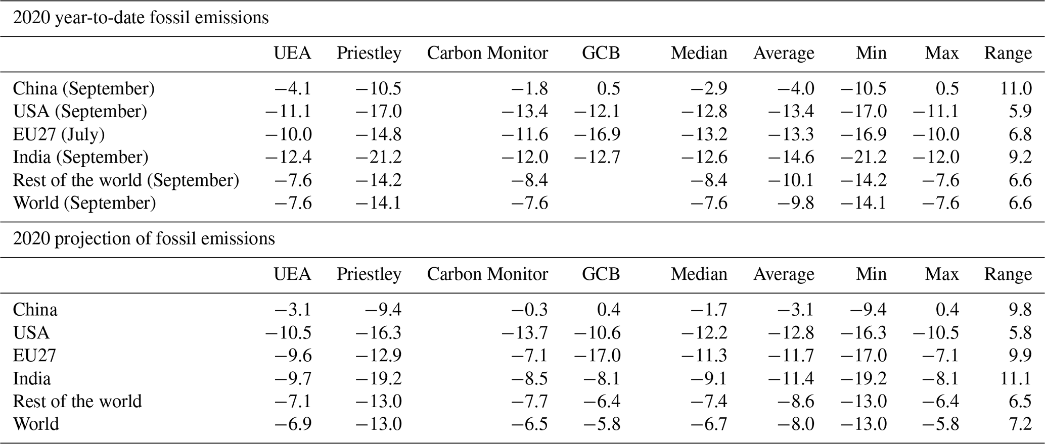
Table A9Funding supporting the production of the various components of the global carbon budget in addition to the authors' supporting institutions (see also acknowledgements).
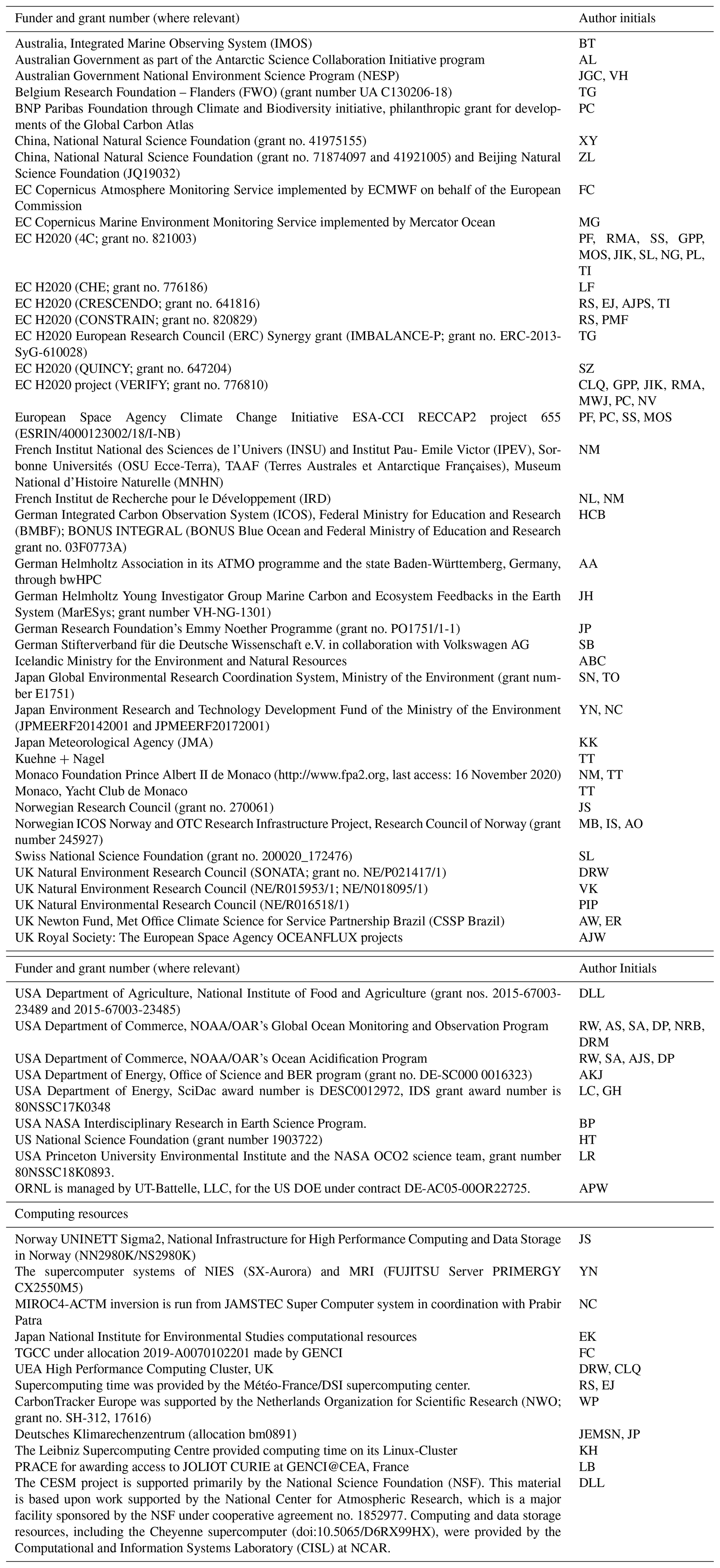
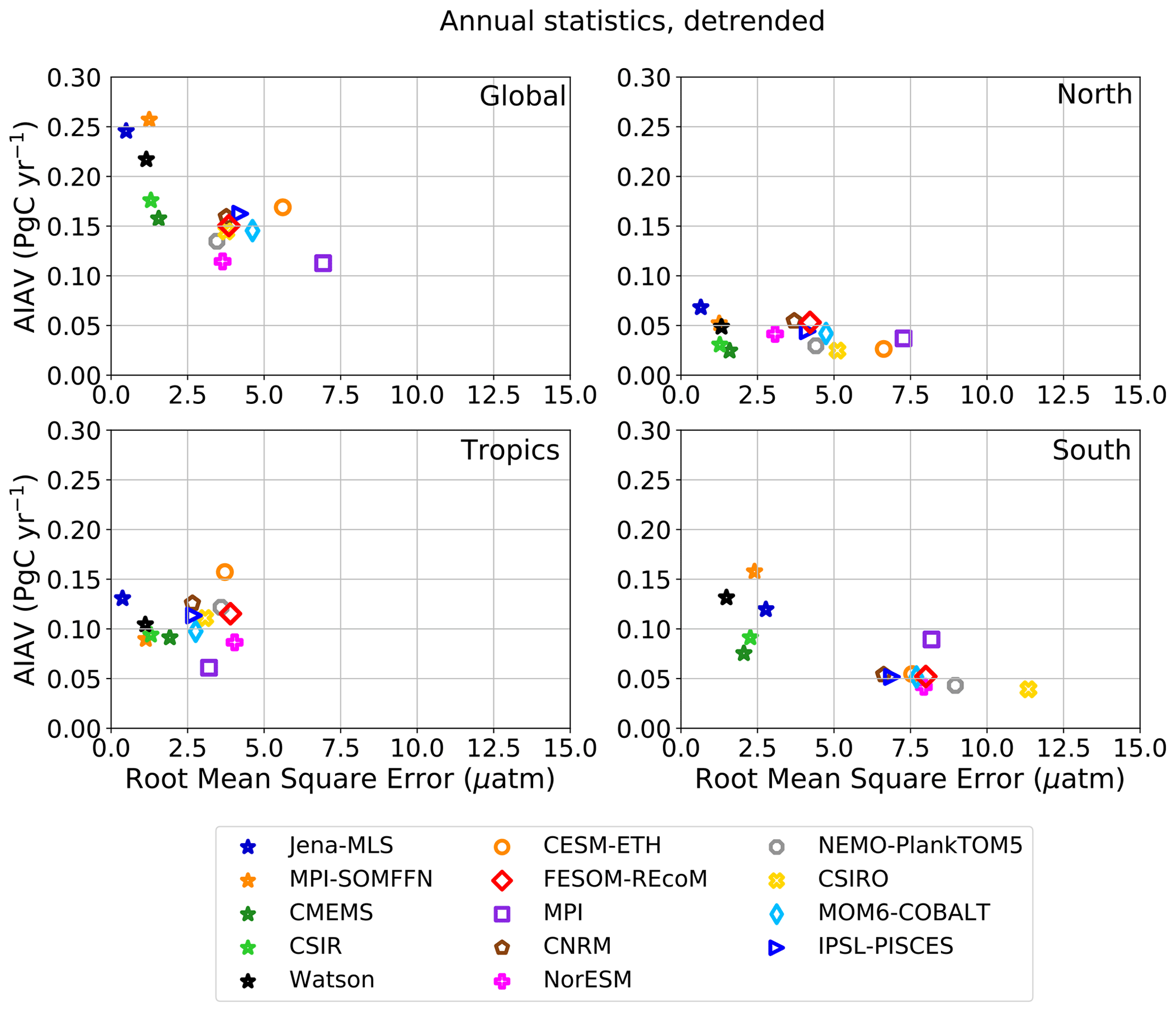
Figure B1Evaluation of the GOBMs and flux products using the root mean squared error (RMSE) for the period 1985 to 2019, between the individual surface ocean pCO2 estimates and the SOCAT v2020 database. The y axis shows the amplitude of the interannual variability (A-IAV, taken as the standard deviation of a detrended time series calculated as a 12-month running mean over the monthly flux time series; Rödenbeck et al., 2015). Results are presented for the globe, north (> 30∘ N), tropics (30∘ S–30∘ N), and south (< 30∘ S) for the GOBMs (see legend circles) and for the pCO2-based flux products (star symbols). The five pCO2-based flux products use the SOCAT database and therefore are not fully independent from the data (see Sect. 2.4.1).
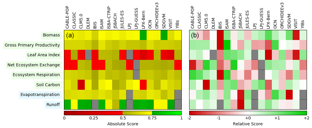
Figure B2Evaluation of the DGVM using the International Land Model Benchmarking system (ILAMB; Collier et al., 2018) (a) absolute skill scores and (b) skill scores relative to other models. The benchmarking is done with observations for vegetation biomass (Saatchi et al., 2011; GlobalCarbon unpublished data; Avitabile et al., 2016), GPP (Jung et al., 2010; Lasslop et al., 2010), leaf area index (De Kauwe et al., 2011; Myneni et al., 1997), net ecosystem exchange (Jung et al., 2010; Lasslop et al., 2010), ecosystem respiration (Jung et al., 2010; Lasslop et al., 2010), soil carbon (Hugelius et al., 2013; Todd-Brown et al., 2013), evapotranspiration (De Kauwe et al., 2011), and runoff (Dai and Trenberth, 2002). For each model–observation comparison a series of error metrics are calculated, scores are then calculated as an exponential function of each error metric, and finally for each variable the multiple scores from different metrics and observational data sets are combined to give the overall variable scores shown in (a). Overall variable scores increase from 0 to 1 with improvements in model performance. The set of error metrics vary with data set and can include metrics based on the period mean, bias, root mean squared error, spatial distribution, interannual variability and seasonal cycle. The relative skill score shown in (b) is a Z score, which indicates in units of standard deviation the model scores relative to the multi-model mean score for a given variable. Grey boxes represent missing model data.

Figure B3Evaluation of the atmospheric inversion products. The mean of the model minus observations is shown for four latitude bands in three periods: (a) 2001–2010, (b) 2011–2018, (c) 2001–2018. The four models are compared to independent CO2 measurements made on board aircraft over many places of the world between 2 and 7 km above sea level. Aircraft measurements archived in the Cooperative Global Atmospheric Data Integration Project (CGADIP, 2020) from sites, campaigns or programs that cover at least 9 months between 2001 and 2018, and that have not been assimilated have been used to compute the biases of the differences in four 45∘ latitude bins. Land and ocean data are used without distinction.
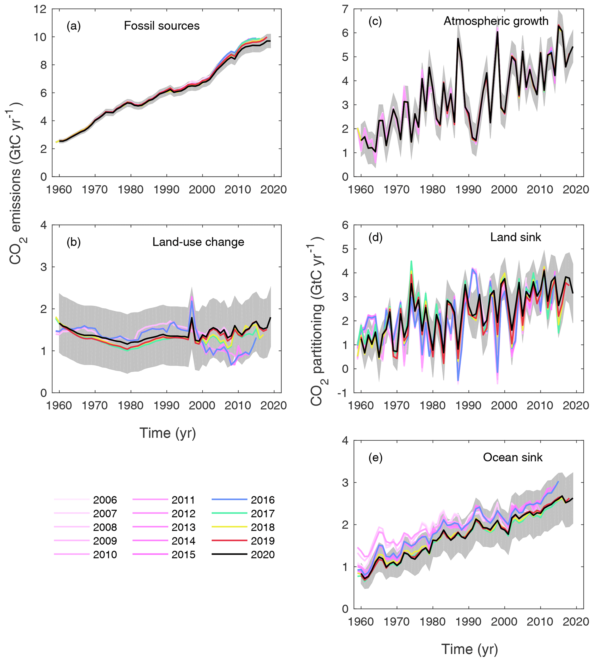
Figure B4Comparison of global carbon budget components released annually by GCP since 2006. CO2 emissions from (a) fossil CO2 emissions (EFOS) and (b) land-use change (ELUC), as well as their partitioning among (c) the atmosphere (GATM), (d) the land (SLAND), and (e) the ocean (SOCEAN). See legend for the corresponding years, and Tables 3 and A7 for references. The budget year corresponds to the year when the budget was first released. All values are in GtC yr−1. Grey shading shows the uncertainty bounds representing ±1σ of the current global carbon budget. Note that the 2020 estimate of EFOS includes the cement carbonation sink.
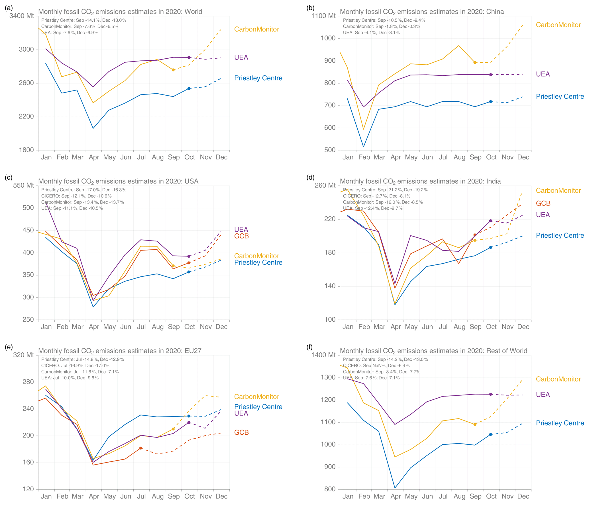
Figure B5Monthly 2020 fossil CO2 emission based on year-to-date data (solid lines) and projections (dashed lines) following four available approaches for (a) the whole world, (b) China, (c) the USA, (d) the European Union, (e) India, and (f) the rest of the world. Methods of the four approaches are described in Sect. 2.1.5 and Appendix C.
C1 Details of the Global Carbon Budget projection method
C1.1 China
The method for the projection uses (1) the sum of monthly domestic production of raw coal, crude oil, natural gas, and cement from the National Bureau of Statistics (NBS, 2020a); (2) monthly net imports of coal, coke, crude oil, refined petroleum products, and natural gas from the General Administration of Customs of the People's Republic of China (2019); and (3) annual energy consumption data by fuel type and annual production data for cement from the NBS, using data for 2000–2018 (NBS, 2019), with the growth rates for 2019 taken from official preliminary statistics for 2019 (NBS, 2020a, b). We estimate the full-year growth rate for 2020 using a Bayesian regression for the ratio between the annual energy consumption data (3 above) from 2014 through 2019, and monthly production plus net imports through August of each year (1+2 above). The uncertainty range uses the standard deviations of the resulting posteriors. Sources of uncertainty and deviations between the monthly and annual growth rates include lack of monthly data on stock changes and energy density, variance in the trend during the last 3 months of the year, and partially unexplained discrepancies between supply-side and consumption data even in the final annual data. The YTD estimate is made in the same way, but instead of regressing the ratio between historical monthly data for August and full-year annual data, monthly data for December are used instead, to produce regression results that capture the systematic differences between the monthly supply and annual consumption data, without the additional effect of projecting forward from August to the end of the year.
Note that in recent years, the absolute value of the annual growth rate for coal energy consumption, and hence total CO2 emissions, has been consistently lower (closer to zero) than the growth or decline suggested by the monthly, tonnage-based production and import data, and this is reflected in the projection. This pattern is only partially explained by stock changes and changes in energy content, and it is therefore not possible to be certain that it will continue in any given year. For 2020 in particular, the COVID-19-related lockdown and reopening in China, similar but delayed restrictions in major export markets, and unusual amounts of flooding and extreme weather during the summer months imply that seasonal patterns and correlations between supply, stock changes, and consumption are likely to be quite different this year than in the previous years that the regression is based on. This adds a major but unquantified amount of uncertainty to the estimate.
C1.2 USA
We use emissions estimated by the US Energy Information Administration (EIA) in their Short-Term Energy Outlook (STEO) for emissions from fossil fuels to get both a YTD and full-year projection (EIA, 2020). The STEO also includes a near-term forecast based on an energy forecasting model which is updated monthly (last update with preliminary data through August 2020) and takes into account expected temperatures, household expenditures by fuel type, energy markets, policies, and other effects. We combine this with our estimate of emissions from cement production using the monthly US cement data from USGS for January–June 2020, assuming changes in cement production over the first part of the year apply throughout the year.
C1.3 India
We use monthly emissions estimates for India updated from Andrew (2020b) through August. These estimates are derived from many official monthly energy and other activity data sources to produce direct estimates of national CO2 emissions, without the use of proxies. For purposes of comparison with other methods, we use a simple approach to extrapolating their observations by assuming the remaining months of the year change by the same relative amount compared to 2019 in the final month of observations.
C1.4 EU
We use (1) monthly coal delivery data from Eurostat for January through June 2020 (Eurostat, 2020); (2) monthly oil and gas demand data for January through June from the Joint Organisations Data Initiative (JODI, 2020), with adjustments for deliveries to petrochemical industries using data from Eurostat (2020); and (3) cement production, which is assumed stable. For purposes of comparison with other methods, we use a simple approach to extrapolating their observations by assuming the remaining months of the year change by the same relative amount compared to 2019 in the final month of observations.
C1.5 Rest of the world
This method only provides a full-year projection. We use the close relationship between the growth in GDP and the growth in emissions (Raupach et al., 2007) to project emissions for the current year. This is based on a simplified Kaya identity, whereby EFOS (GtC yr−1) is decomposed by the product of GDP (USD yr−1) and the fossil fuel carbon intensity of the economy (IFOS; GtC USD−1) as follows:
Taking a time derivative of Eq. (3) and rearranging gives
where the left-hand term is the relative growth rate of EFOS, and the right-hand terms are the relative growth rates of GDP and IFOS, respectively, which can simply be added linearly to give the overall growth rate.
The IFOS is based on GDP in constant PPP (purchasing power parity) from the International Energy Agency (IEA) up to 2017 (IEA/OECD, 2019) and extended using the International Monetary Fund (IMF) growth rates through 2019 (IMF, 2020). Interannual variability in IFOS is the largest source of uncertainty in the GDP-based emissions projections. We thus use the standard deviation of the annual IFOS for the period 2009–2019 as a measure of uncertainty, reflecting a ±1σ as in the rest of the carbon budget.
C1.6 World
This method only provides a full-year projection. The global total is the sum of each of the countries and regions, but this year we additionally apply a GDP approach to the world to provide an additional consistency check (see “rest of world” description).
PF, MOS, MWJ, CLQ, RMA, JH, GPP, WP, JP, SS, AO, JGC, PC, and RBJ designed the study, conducted the analysis, and wrote the paper. RMA, GPP, and JIK produced the emissions, their uncertainties, and the GCB 2020 emission projections and analysed the emissions data. DG and GM provided emission data. PPT provided key atmospheric CO2 data. WP, PC, FC, CR, NC, YN, PIP, and LF provided an updated atmospheric inversion, developed the protocol, and produced the evaluation. JP, KH, SB, TG, and RAH provided updated bookkeeping land-use change emissions. LPC, LEOCA, and GRvdW provided forcing data for land-use change. AA, VH, AKJ, EJ, EK, SL, DLL, JRM, JEMSN, BP, HT, NV, APW, AJW, WY, XY, and SZ provided an update of a DGVM. IH provided the climate forcing data for the DGVMs. ER provided the evaluation of the DGVMs. JH, LB, NG, TI, AL, LR, JS, RS, and DW provided an update of a GOBM. MG, LG, PL, CR, and AJW provided an update of an ocean flux product. SA, NRB, MB, AB, HCB, WE, TG, KK, VK, NL, NM, DRM, SN, KO, AO, TO, DP, IS, AJS, TT, BT, and RW provided ocean pCO2 measurements for the year 2019, with synthesis by AO and KO. PF, MOS, and MWJ revised all figures, tables, text, and/or numbers to ensure the update is clear from the 2019 edition and in phase with the globalcarbonatlas.org.
The authors declare that they have no conflict of interest.
We thank all people and institutions who provided the data used in this carbon budget and Ian G. C. Ashton, Matthew Chamberlain, Ed Chan, Laique Djeutchouang, Christian Ethé, Liang Feng, Matthew Fortier, Lonneke Goddijn-Murphy, Thomas Holding, George Hurtt, Joe Melton, Tristan Quaife, Marine Remaud, Shijie Shu, Jamie Shutler, Anthony Walker, Ulrich Weber, and David K. Woolf for their involvement in the development, use, and analysis of the models and data products used here. We thank Ed Dlugokencky for providing atmospheric CO2 measurements; We thank Benjamin Pfeil, Steve Jones, Rocío Castaño-Primo, and Maren Karlsen of the Ocean Thematic Centre of the EU Integrated Carbon Observation System (ICOS) Research Infrastructure for their contribution, as well as Karl Smith of NOAA's Pacific Marine Environmental Laboratory and Kim Currie, Joe Salisbury, Doug Vandermark, Chris Hunt, Douglas Wallace, and Dariia Atamanchuck, who contributed to the provision of ocean pCO2 observations for the year 2019 (see Table A5). This is NOAA-PMEL contribution number 5167. We thank the institutions and funding agencies responsible for the collection and quality control of the data in SOCAT, and the International Ocean Carbon Coordination Project (IOCCP) for its support. We thank the FAO and its member countries for the collection and free dissemination of data relevant to this work. We thank data providers ObsPack GLOBALVIEWplus v5.0 and NRT v5.2 for atmospheric CO2 observations. We thank Trang Chau who produced the CMEMS pCO2-based ocean flux data and designed the system together with Marion Gehlen, Anna Denvil-Sommer, and Frédéric Chevallier1. We thank the individuals and institutions that provided the databases used for the model evaluations introduced here, and Nigel Hawtin for producing Figs. 2 and 9. We thank all the scientists, software engineers, and administrators who contributed to the development of CESM2. We thank Fortunat Joos, Samar Khatiwala, and Timothy DeVries for providing historical data. We thank all people and institutions who provided the data used in this carbon budget and the Global Carbon Project members for their input throughout the development of this update. Finally, we thank all funders who have supported the individual and joint contributions to this work (see Table A9), as well as the reviewers of this paper and previous versions, and the many researchers who have provided feedback.
For a list of all funders that have supported this research, please refer to Table A9.
This paper was edited by David Carlson and reviewed by Albertus J. (Han) Dolman, Tomohiro Oda and two anonymous referees.
Amante, C. and Eakins, B. W.: ETOPO1 1 Arc-Minute Global Relief Model: Procedures, Data Sources and Analysis, NOAA Technical Memorandum NESDIS NGDC-24, National Geophysical Data Center, NOAA, https://doi.org/10.7289/V5C8276M, 2009.
Andres, R. J., Boden, T. A., Bréon, F.-M., Ciais, P., Davis, S., Erickson, D., Gregg, J. S., Jacobson, A., Marland, G., Miller, J., Oda, T., Olivier, J. G. J., Raupach, M. R., Rayner, P., and Treanton, K.: A synthesis of carbon dioxide emissions from fossil-fuel combustion, Biogeosciences, 9, 1845–1871, https://doi.org/10.5194/bg-9-1845-2012, 2012.
Andres, R. J., Boden, T. A., and Higdon, D.: A new evaluation of the uncertainty associated with CDIAC estimates of fossil fuel carbon dioxide emission, Tellus B, 66, 23616, https://doi.org/10.3402/tellusb.v66.23616, 2014.
Andrew, R. M.: Global CO2 emissions from cement production, 1928–2018, Earth Syst. Sci. Data, 11, 1675–1710, https://doi.org/10.5194/essd-11-1675-2019, 2019.
Andrew, R. M.: A comparison of estimates of global carbon dioxide emissions from fossil carbon sources, Earth Syst. Sci. Data, 12, 1437–1465, https://doi.org/10.5194/essd-12-1437-2020, 2020a.
Andrew, R. M.: Timely estimates of India's annual and monthly fossil CO2 emissions, Earth Syst. Sci. Data, 12, 2411–2421, https://doi.org/10.5194/essd-12-2411-2020, 2020b.
Andrew, R. M. and Peters, G. P.: A Multi-Region Input-Output Table Based on the Global Trade Analysis Project Database (Gtap-Mrio), Econ. Syst. Res., 25, 99–121, https://doi.org/10.1080/09535314.2012.761953, 2013.
Archer, D., Eby, M., Brovkin, V., Ridgwell, A., Cao, L., Mikolajewicz, U., Caldeira, K., Matsumoto, K., Munhoven, G., Montenegro, A., and Tokos, K.: Atmospheric Lifetime of Fossil Fuel Carbon Dioxide, Annu. Rev. Earth Pl. Sc., 37, 117–134, https://doi.org/10.1146/annurev.earth.031208.100206, 2009.
Arneth, A., Sitch, S., Pongratz, J., Stocker, B. D., Ciais, P., Poulter, B., Bayer, A. D., Bondeau, A., Calle, L., Chini, L. P., Gasser, T., Fader, M., Friedlingstein, P., Kato, E., Li, W., Lindeskog, M., Nabel, J. E. M. S., Pugh, T. A. M., Robertson, E., Viovy, N., Yue, C., and Zaehle, S.: Historical carbon dioxide emissions caused by land-use changes are possibly larger than assumed, Nat. Geosci., 10, 79–84, https://doi.org/10.1038/ngeo2882, 2017.
Arora, V. K., Boer, G. J., Christian, J. R., Curry, C. L., Denman, K. L., Zahariev, K., Flato, G. M., Scinocca, J. F., Merryfield, W. J., and Lee, W. G.: The Effect of Terrestrial Photosynthesis Down Regulation on the Twentieth-Century Carbon Budget Simulated with the CCCma Earth System Model, J. Climate, 22, 6066–6088, https://doi.org/10.1175/2009jcli3037.1, 2009.
Aumont, O., Orr, J. C., Monfray, P., Ludwig, W., Amiotte-Suchet, P., and Probst, J. L.: Riverine-driven interhemispheric transport of carbon, Global Biogeochem. Cy., 15, 393–405, https://doi.org/10.1029/1999GB001238, 2001.
Aumont, O., Ethé, C., Tagliabue, A., Bopp, L., and Gehlen, M.: PISCES-v2: an ocean biogeochemical model for carbon and ecosystem studies, Geosci. Model Dev., 8, 2465–2513, https://doi.org/10.5194/gmd-8-2465-2015, 2015.
Avitabile, V., Herold, M., Heuvelink, G. B. M., Lewis, S. L., Phillips, O. L., Asner, G. P., Armston, J., Ashton, P. S., Banin, L., Bayol, N., Berry, N. J., Boeckx, P., de Jong, B. H. J., DeVries, B., Girardin, C. A. J., Kearsley, E., Lindsell, J. A., Lopez-Gonzalez, G., Lucas, R., Malhi, Y., Morel, A., Mitchard, E. T. A., Nagy, L., Qie, L., Quinones, M. J., Ryan, C. M., Ferry, S. J. W., Sunderland, T., Laurin, G. V., Gatti, R. C., Valentini, R., Verbeeck, H., Wijaya, A., and Willcock, S.: An integrated pan-tropical biomass map using multiple reference datasets, Glob. Change Biol., 22, 1406–1420, https://doi.org/10.1111/gcb.13139, 2016.
Baccini, A., Walker, W., Carvalho, L., Farina, M., Sulla-Menashe, D., and Houghton, R. A.: Tropical forests are a net carbon source based on aboveground measurements of gain and loss, Science, 358, 230–234, https://doi.org/10.1126/science.aam5962, 2017.
Bakker, D. C. E., Pfeil, B., Landa, C. S., Metzl, N., O'Brien, K. M., Olsen, A., Smith, K., Cosca, C., Harasawa, S., Jones, S. D., Nakaoka, S., Nojiri, Y., Schuster, U., Steinhoff, T., Sweeney, C., Takahashi, T., Tilbrook, B., Wada, C., Wanninkhof, R., Alin, S. R., Balestrini, C. F., Barbero, L., Bates, N. R., Bianchi, A. A., Bonou, F., Boutin, J., Bozec, Y., Burger, E. F., Cai, W.-J., Castle, R. D., Chen, L., Chierici, M., Currie, K., Evans, W., Featherstone, C., Feely, R. A., Fransson, A., Goyet, C., Greenwood, N., Gregor, L., Hankin, S., Hardman-Mountford, N. J., Harlay, J., Hauck, J., Hoppema, M., Humphreys, M. P., Hunt, C. W., Huss, B., Ibánhez, J. S. P., Johannessen, T., Keeling, R., Kitidis, V., Körtzinger, A., Kozyr, A., Krasakopoulou, E., Kuwata, A., Landschützer, P., Lauvset, S. K., Lefèvre, N., Lo Monaco, C., Manke, A., Mathis, J. T., Merlivat, L., Millero, F. J., Monteiro, P. M. S., Munro, D. R., Murata, A., Newberger, T., Omar, A. M., Ono, T., Paterson, K., Pearce, D., Pierrot, D., Robbins, L. L., Saito, S., Salisbury, J., Schlitzer, R., Schneider, B., Schweitzer, R., Sieger, R., Skjelvan, I., Sullivan, K. F., Sutherland, S. C., Sutton, A. J., Tadokoro, K., Telszewski, M., Tuma, M., van Heuven, S. M. A. C., Vandemark, D., Ward, B., Watson, A. J., and Xu, S.: A multi-decade record of high-quality fCO2 data in version 3 of the Surface Ocean CO2 Atlas (SOCAT), Earth Syst. Sci. Data, 8, 383–413, https://doi.org/10.5194/essd-8-383-2016, 2016.
Bakker, D. C. E., Alin, S. R., Bates, N., Becker, M., Castaño-Primo, R., Cosca, C. E., Cronin, M., Kadono, K., Kozyr, A., Lauvset, S. K., Metzl, N., Munro, D. R., Nakaoka, S., O'Brien, K. M., Ólafsson, J., Olsen, A., Pfeil, B., Pierrot, D., Smith, K., Sutton, A. J., Takahashi, T., Tilbrook, B., Wanninkhof, R., Andersson, A., Atamanchuk, D., Benoit-Cattin, A., Bott, R., Burger, E. F., Cai, W.-J., Cantoni, C., Collins, A., Corredor, J. E., Cronin, M. F., Cross, J. N, Currie, K. I., De Carlo, E. H., DeGrandpre, M. D., Dietrich, C., Emerson, S., Enright, M. P., Evans, W., Feely, R. A., García-Ibáñez, M. I., Gkritzalis, T., Glockzin, M., Hales, B., Hartman, S. E., Hashida, G., Herndon, J., Howden, S. D., Humphreys, M. P., Hunt, C. W., Jones, S. D., Kim, S., Kitidis, V., Landa, C. S, Landschützer, P., Lebon, G. T., Lefèvre, N., Lo Monaco, C., Luchetta, A., Maenner Jones, S., Manke, A. B., Manzello, D., Mears, P., Mickett, J., Monacci, N. M., Morell, J. M., Musielewicz, S., Newberger, T., Newton, J., Noakes, S., Noh, J.-H., Nojiri, Y., Ohman, M., Ólafsdóttir, S., Omar, A. M., Ono, T., Osborne, J., Plueddemann, A. J., Rehder, G., Sabine, C. L, Salisbury, J. E., Schlitzer, R., Send, U., Skjelvan, I., Sparnocchia, S., Steinhoff, T., Sullivan, K. F., Sutherland, S. C., Sweeney, C., Tadokoro, K., Tanhua, T., Telszewski, M., Tomlinson, M., Tribollet, A., Trull, T., Vandemark, D., Wada, C., Wallace, D. W. R., Weller, R. A., and Woosley, R. J.: Surface Ocean CO2 Atlas Database Version 2020 (SOCATv2020) (NCEI Accession 0210711), NOAA National Centers for Environmental Information, https://doi.org/10.25921/4xkx-ss49. 2020.
Ballantyne, A. P., Alden, C. B., Miller, J. B., Tans, P. P., and White, J. W. C.: Increase in observed net carbon dioxide uptake by land and oceans during the past 50 years, Nature, 488, 70–72, https://doi.org/10.1038/nature11299, 2012.
Ballantyne, A. P., Andres, R., Houghton, R., Stocker, B. D., Wanninkhof, R., Anderegg, W., Cooper, L. A., DeGrandpre, M., Tans, P. P., Miller, J. B., Alden, C., and White, J. W. C.: Audit of the global carbon budget: estimate errors and their impact on uptake uncertainty, Biogeosciences, 12, 2565–2584, https://doi.org/10.5194/bg-12-2565-2015, 2015.
Bastos, A., O'Sullivan, M., Ciais, P., Makowski, D., Sitch, S., Friedlingstein, P., Chevallier, F., Rödenbeck, C., Pongratz, J., Luijkx, I. T., Patra, P. K., Peylin, P., Canadell, J. G., Lauerwald, R., Li, W., Smith, N. E., Peters, W., Goll, D. S., Jain, A. K., Kato, E., Lienert, S., Lombardozzi, D. L., Haverd, V., Nabel, J. E. M. S., Poulter, B., Tian, H., Walker, A. P., and Zaehle, S.: Sources of Uncertainty in Regional and Global Terrestrial CO2 Exchange Estimates, Global Biogeochem. Cycles, 34, 1–21, https://doi.org/10.1029/2019GB006393, 2020.
Basu, S., Baker, D. F., Chevallier, F., Patra, P. K., Liu, J., and Miller, J. B.: The impact of transport model differences on CO2 surface flux estimates from OCO-2 retrievals of column average CO2, Atmos. Chem. Phys., 18, 7189–7215, https://doi.org/10.5194/acp-18-7189-2018, 2018.
Bauer, J. E., Cai, W.-J., Raymond, P. a, Bianchi, T. S., Hopkinson, C. S. and Regnier, P. G.: The changing carbon cycle of the coastal ocean, Nature, 504, 61–70, https://doi.org/10.1038/nature12857, 2013.
Berthet, S., Séférian, R., Bricaud, C., Chevallier, M., Voldoire, A., and Ethé, C.: Evaluation of an Online Grid-Coarsening Algorithm in a Global Eddy-Admitting Ocean Biogeochemical Model, J. Adv. Model. Earth Sy., 11, 1759–1783, https://doi.org/10.1029/2019MS001644, 2019.
Best, M. J., Pryor, M., Clark, D. B., Rooney, G. G., Essery, R. L. H., Ménard, C. B., Edwards, J. M., Hendry, M. A., Porson, A., Gedney, N., Mercado, L. M., Sitch, S., Blyth, E., Boucher, O., Cox, P. M., Grimmond, C. S. B., and Harding, R. J.: The Joint UK Land Environment Simulator (JULES), model description – Part 1: Energy and water fluxes, Geosci. Model Dev., 4, 677–699, https://doi.org/10.5194/gmd-4-677-2011, 2011.
BP: BP Statistical Review of World Energy June 2020, available at: https://www.bp.com/en/global/corporate/energy-economics/statistical-review-of-world-energy.html, last access: 16 November 2020.
Broecker, W. S., Spencer, D. W., and Craig, H. C.: GEOSECS Pacific Expedition: Hydrographic data 1973–1974, PANGAEA, https://doi.org/10.1594/PANGAEA.824127, 1982.
Bruno, M. and Joos, F.: Terrestrial carbon storage during the past 200 years: A Monte Carlo Analysis of CO2 data from ice core and atmospheric measurements, Global Biogeochem. Cy., 11, 111–124, https://doi.org/10.1029/96GB03611, 1997.
Buitenhuis, E. T., Hashioka, T., and Le Quéré, C.: Combined constraints on global ocean primary production using observations and models, Global Biogeochem. Cy., 27, 847–858, https://doi.org/10.1002/gbc.20074, 2013.
Bushinsky, S. M., Landschützer, P., Rödenbeck, C., Gray, A. R., Baker, D., Mazloff, M. R., Resplandy, L., Johnson, K. S., and Sarmiento, J. L.: Reassessing Southern Ocean Air‐Sea CO2 Flux Estimates With the Addition of Biogeochemical Float Observations, Global Biogeochem. Cycles, 33, 1370–1388, https://doi.org/10.1029/2019GB006176, 2019.
Canadell, J. G., Le Quéré, C., Raupach, M. R., Field, C. B., Buitenhuis, E. T., Ciais, P., Conway, T. J., Gillett, N. P., Houghton, R. A., and Marland, G.: Contributions to accelerating atmospheric CO2 growth from economic activity, carbon intensity, and efficiency of natural sinks, P. Natl. Acad. Sci. USA, 104, 18866–18870, https://doi.org/10.1073/pnas.0702737104, 2007.
Cao, Z., Myers, R. J., Lupton, R. C., Duan, H., Sacchi, R., Zhou, N., Reed Miller, T., Cullen, J. M., Ge, Q., and Liu, G.: The sponge effect and carbon emission mitigation potentials of the global cement cycle, Nat. Commun., 11, 1–9, https://doi.org/10.1038/s41467-020-17583-w, 2020.
Carbontracker Team: obspack_co2_1_NRT_v5.2_2020-06-03, available at: https://www.esrl.noaa.gov/gmd/ccgg/obspack/release_notes.html, last access: 16 November 2020.
CGADIP: obspack_co2_1_GLOBALVIEWplus_v5.0_2019-08-12, available at: https://www.esrl.noaa.gov/gmd/ccgg/obspack/release_notes.html, last access: 16 November 2020.
Chatfield, C.: The Holt-Winters Forecasting Procedure, Appl. Stat., 27, 264–279, https://doi.org/10.2307/2347162, 1978.
Chau, T. T., Gehlen, M., and Chevallier, F.: Global Ocean Surface Carbon Product MULTIOBS_GLO_BIO_CARBON_SURFACE_REP_015_008, E.U. Copernicus Marine Service Information, available at: https://resources.marine.copernicus.eu/?option=com_cswandview=detailsandproduct_id=MULTIOBS_G, last access: 16 November 2020.
Chevallier, F.: On the parallelization of atmospheric inversions of CO2 surface fluxes within a variational framework, Geosci. Model Dev., 6, 783–790, https://doi.org/10.5194/gmd-6-783-2013, 2013.
Chevallier, F., Fisher, M., Peylin, P., Serrar, S., Bousquet, P., Bréon, F.-M., Chédin, A., and Ciais, P.: Inferring CO2 sources and sinks from satellite observations: Method and application to TOVS data, J. Geophys. Res., 110, D24309, https://doi.org/10.1029/2005JD006390, 2005.
Chevallier, F., Remaud, M., O'Dell, C. W., Baker, D., Peylin, P., and Cozic, A.: Objective evaluation of surface- and satellite-driven carbon dioxide atmospheric inversions, Atmos. Chem. Phys., 19, 14233–14251, https://doi.org/10.5194/acp-19-14233-2019, 2019.
Ciais, P., Sabine, C., Bala, G., Bopp, L., Brovkin, V., Canadell, J., Chhabra, A., DeFries, R., Galloway, J., Heimann, M., Jones, C., Le Quéré, C., Myneni, R. B., Piao, S., Thornton, P., Willem, J., Friedlingstein, P., and Munhoven, G.: Carbon and Other Biogeochemical Cycles, in Climate Change 2013: The Physical Science Basis, Contribution of Working Group I to the Fifth Assessment Report of the Intergovernmental Panel on Climate Change, edited by: Intergovernmental Panel on Climate Change, Cambridge University Press, Cambridge, UK, 465–570, 2013.
Ciais, P., Tan, J., Wang, X., Roedenbeck, C., Chevallier, F., Piao, S. L., Moriarty, R., Broquet, G., Le Quéré, C., Canadell, J. G., Peng, S., Poulter, B., Liu, Z., and Tans, P.: Five decades of northern land carbon uptake revealed by the interhemispheric CO2 gradient, Nature, 568, 221–225, https://doi.org/10.1038/s41586-019-1078-6, 2019.
Clark, D. B., Mercado, L. M., Sitch, S., Jones, C. D., Gedney, N., Best, M. J., Pryor, M., Rooney, G. G., Essery, R. L. H., Blyth, E., Boucher, O., Harding, R. J., Huntingford, C., and Cox, P. M.: The Joint UK Land Environment Simulator (JULES), model description – Part 2: Carbon fluxes and vegetation dynamics, Geosci. Model Dev., 4, 701–722, https://doi.org/10.5194/gmd-4-701-2011, 2011.
Collier, N., Hoffman, F. M., Lawrence, D. M., Keppel-Aleks, G., Koven, C. D., Riley, W. J., Mu, M. Q., and Randerson, J. T.: The International Land Model Benchmarking (ILAMB) System: Design, Theory, and Implementation, J. Adv. Model. Earth Sy., 10, 2731–2754, https://doi.org/10.1029/2018ms001354, 2018.
Conchedda, G. and Tubiello, F. N.: Drainage of organic soils and GHG emissions: Validation with country data, Earth Syst. Sci. Data Discuss., https://doi.org/10.5194/essd-2020-202, in review, 2020.
Cooper, D. J., Watson, A. J., and Ling, R. D.: Variation of pCO2 along a North Atlantic shipping route (U.K. to the Caribbean): A year of automated observations, Mar. Chem., 60, 147–164, https://doi.org/10.1016/S0304-4203(97)00082-0, 1998.
Cox, P. M., Pearson, D., Booth, B. B., Friedlingstein, P., Huntingford, C., Jones, C. D., and Luke, C. M.: Sensitivity of tropical carbon to climate change constrained by carbon dioxide variability, Nature, 494, 341–344, https://doi.org/10.1038/nature11882, 2013.
Crippa, M., Oreggioni, G., Guizzardi, D., Muntean, M., Schaaf, E., Lo Vullo, E., Solazzo, E., Monforti-Ferrario, F., Olivier, J. G. J., and Vignati, E.: Fossil CO2 and GHG emissions of all world countries, EUR 29849 EN, Luxembourg, JRC117610, Publications Office of the European Union, 2019.
Dai, A. and Trenberth, K. E.: Estimates of Freshwater Discharge from Continents: Latitudinal and Seasonal Variations, J. Hydrometeorol., 3, 660–687, https://doi.org/10.1175/1525-7541(2002)003<0660:EOFDFC>2.0.CO;2, 2002.
Davis, S. J. and Caldeira, K.: Consumption-based accounting of CO2 emissions, P. Natl. Acad. Sci. USA, 107, 5687–5692, https://doi.org/10.1073/pnas.0906974107, 2010.
Decharme, B., Delire, C., Minvielle, M., Colin, J., Vergnes, J., Alias, A., Saint-Martin, D., Séférian, R., Sénési, S., and Voldoire, A.: Recent Changes in the ISBA-CTRIP Land Surface System for Use in the CNRM-CM6 Climate Model and in Global Off-Line Hydrological Applications, J. Adv. Model. Earth Sy., 11, 1207–1252, https://doi.org/10.1029/2018MS001545, 2019.
De Kauwe, M. G., Disney, M. I., Quaife, T., Lewis, P., and Williams, M.: An assessment of the MODIS collection 5 leaf area index product for a region of mixed coniferous forest, Remote Sens. Environ., 115, 767–780, https://doi.org/10.1016/j.rse.2010.11.004, 2011.
Delire, C., Séférian, R., Decharme, B., Alkama, R., Calvet, J., Carrer, D., Gibelin, A., Joetzjer, E., Morel, X., Rocher, M., and Tzanos, D.: The Global Land Carbon Cycle Simulated With ISBA-CTRIP: Improvements Over the Last Decade, J. Adv. Model. Earth Sy., 12, e2019MS001886, https://doi.org/10.1029/2019MS001886, 2020.
Denman, K. L., Brasseur, G., Chidthaisong, A., Ciais, P., Cox, P. M., Dickinson, R. E., Hauglustaine, D., Heinze, C., Holland, E., Jacob, D., Lohmann, U., Ramachandran, S., Leite da Silva Dias, P., Wofsy, S. C., and Zhang, X.: Couplings Between Changes in the Climate System and Biogeochemistry, in: Climate Change 2007: The Physical Science Basis. Contribution of Working Group I to the Fourth Assessment Report of the Intergovernmental Panel on Climate Change, edited by: Solomon, S., Qin, D., Manning, M., Marquis, M., Averyt, K., Tignor, M. M. B., Miller, H. L., and Chen, Z. L., Cambridge University Press, Cambridge, UK and New York, USA, 499–587, 2007.
Denning, A. S., Fung, I. Y., and Randall, D.: Latitudinal gradient of atmospheric CO2 due to seasonal exchange with land biota, Nature, 376, 240–243, https://doi.org/10.1038/376240a0, 1995.
Denvil-Sommer, A., Gehlen, M., Vrac, M., and Mejia, C.: LSCE-FFNN-v1: a two-step neural network model for the reconstruction of surface ocean pCO2 over the global ocean, Geosci. Model Dev., 12, 2091–2105, https://doi.org/10.5194/gmd-12-2091-2019, 2019.
Department of the Environment and Energy: Australian Energy Update 2020, available at: https://www.energy.gov.au/publications/australian-energy-update-2020, last access: 16 November 2020.
DeVries, T.: The oceanic anthropogenic CO2 sink: Storage, air-sea fluxes, and transports over the industrial era, Global Biogeochem. Cy., 28, 631–647, https://doi.org/10.1002/2013gb004739, 2014.
DeVries, T., Holzer, M., and Primeau, F.: Recent increase in oceanic carbon uptake driven by weaker upper-ocean overturning, Nature, 542, 215–218, https://doi.org/10.1038/nature21068, 2017.
DeVries, T., Le Quéré, C., Andrews, O., Berthet, S., Hauck, J., Ilyina, T., Landschützer, P., Lenton, A., Lima, I. D., Nowicki, M., Schwinger, J., and Séférian, R.: Decadal trends in the ocean carbon sink, P. Natl. Acad. Sci. USA, 116, 11646–11651, https://doi.org/10.1073/pnas.1900371116, 2019.
Dickson, A. G., Sabine, C. L., and Christian, J.: Guide to best practices for ocean CO2 measurements, Sidney, British Columbia, North Pacific Marine Science Organization, PICES Special Publication, 3, 176 pp., 2007.
Dlugokencky, E. and Tans, P.: Trends in atmospheric carbon dioxide, National Oceanic and Atmospheric Administration, Earth System Research Laboratory (NOAA/ESRL), available at: http://www.esrl.noaa.gov/gmd/ccgg/trends/global.html, last access: 16 November 2020.
Doney, S. C., Lima, I., Feely, R. A., Glover, D. M., Lindsay, K., Mahowald, N., Moore, J. K., and Wanninkhof, R.: Mechanisms governing interannual variability in upper-ocean inorganic carbon system and air-sea CO2 fluxes: Physical climate and atmospheric dust, Deep-Sea Res. Pt. II, 56, 640–655, https://doi.org/10.1016/j.dsr2.2008.12.006, 2009.
Duce, R. A., LaRoche, J., Altieri, K., Arrigo, K. R., Baker, A. R., Capone, D. G., Cornell, S., Dentener, F., Galloway, J., Ganeshram, R. S., Geider, R. J., Jickells, T., Kuypers, M. M., Langlois, R., Liss, P. S., Liu, S. M., Middelburg, J. J., Moore, C. M., Nickovic, S., Oschlies, A., Pedersen, T., Prospero, J., Schlitzer, R., Seitzinger, S., Sorensen, L. L., Uematsu, M., Ulloa, O., Voss, M., Ward, B., and Zamora, L.: Impacts of Atmospheric Anthropogenic Nitrogen on the Open Ocean, Science, 320, 893–897, https://doi.org/10.1126/science.1150369, 2008.
Dufour, C. O., Le Sommer, J., Gehlen, M., Orr, J. C., Molines, J. M., Simeon, J., and Barnier, B.: Eddy compensation and controls of the enhanced sea-to-air CO2 flux during positive phases of the Southern Annular Mode, Global Biogeochem. Cy., 27, 950–961, https://doi.org/10.1002/gbc.20090, 2013.
Eakins, B. W. and Sharman, G. F.: Volumes of the World's Oceans from ETOPO1, NOAA National Geophysical Data Center, available at: http://www.ngdc.noaa.gov/mgg/global/etopo1_ocean_ volumes.html (last accessed: 16 November 2019), 2010.
EIA: U.S. Energy Information Administration, Short-Term Energy Outlook, available at: http://www.eia.gov/forecasts/steo/outlook.cfm, last access: 16 November 2020.
Erb, K., Kastner, T., Plutzar, C., Bais, A. L. S., Carvalhais, N., Fetzel, T., Gingrich, S., Haberl, H., Lauk, C., Niedertscheider, M., Pongratz, J., Thurner, M., and Luyssaert, S.: Unexpectedly large impact of forest management and grazing on global vegetation biomass, Nature, 553, 73–76, https://doi.org/10.1038/nature25138, 2018.
Erb, K. H., Kastner, T., Luyssaert, S., Houghton, R. A., Kuemmerle, T., Olofsson, P., and Haberl, H.: COMMENTARY: Bias in the attribution of forest carbon sinks, Nat. Clim. Chang., 3, 854–856, https://doi.org/10.1038/nclimate2004, 2013.
Etheridge, D. M., Steele, L. P., Langenfelds, R. L., Francey, R. J., Barnola, J. M., and Morgan, V. I.: Natural and anthropogenic changes in atmospheric CO2 over the last 1000 years from air in Antarctic ice and firn, J. Geophys. Res., 101, 4115–4128, doi:Doi 10.1029/95jd03410, 1996.
Eurostat: Supply and transformation of solid fuels – monthly data (nrg_101m), available at: https://ec.europa.eu/eurostat/data/database, last access: 16 November 2020.
Eyring, V., Bony, S., Meehl, G. A., Senior, C. A., Stevens, B., Stouffer, R. J., and Taylor, K. E.: Overview of the Coupled Model Intercomparison Project Phase 6 (CMIP6) experimental design and organization, Geosci. Model Dev., 9, 1937–1958, https://doi.org/10.5194/gmd-9-1937-2016, 2016.
FAO: AQUASTAT, FAO's global water information system, Online database, available at: http://www.fao.org/nr/water/aquastat/sets/index.stm{#}sed, last access: 12 September 2015.
FAOSTAT: Food and Agriculture Organization Statistics Division, available at: http://faostat.fao.org/ (last access: 16 November 2020), 2015.
Fay, A. R. and McKinley, G. A.: Global open-ocean biomes: mean and temporal variability, Earth Syst. Sci. Data, 6, 273–284, https://doi.org/10.5194/essd-6-273-2014, 2014.
Feng, L., Palmer, P. I., Bösch, H., and Dance, S.: Estimating surface CO2 fluxes from space-borne CO2 dry air mole fraction observations using an ensemble Kalman Filter, Atmos. Chem. Phys., 9, 2619–2633, https://doi.org/10.5194/acp-9-2619-2009, 2009.
Feng, L., Palmer, P. I., Parker, R. J., Deutscher, N. M., Feist, D. G., Kivi, R., Morino, I., and Sussmann, R.: Estimates of European uptake of CO2 inferred from GOSAT XCO2 retrievals: sensitivity to measurement bias inside and outside Europe, Atmos. Chem. Phys., 16, 1289–1302, https://doi.org/10.5194/acp-16-1289-2016, 2016.
Forster, P. M., Forster, H. I., Evans, M. J., Gidden, M. J., Jones, C. D., Keller, C. A., Lamboll, R. D., Le Quéré, C., Rogelj, J., Rosen, D., Schleussner, C., Richardson, T. B., Smith, C. J., and Turnock, S. T.: Current and future global climate impacts resulting from COVID-19, Nat. Clim. Change, 10, 913–919, https://doi.org/10.1038/s41558-020-0883-0, 2020.
Friedlingstein, P., Houghton, R. A., Marland, G., Hackler, J., Boden, T. A., Conway, T. J., Canadell, J. G., Raupach, M. R., Ciais, P., and Le Quéré, C.: Update on CO2 emissions, Nat. Geosci., 3, 811–812, https://doi.org/10.1038/ngeo1022, 2010.
Friedlingstein, P., Andrew, R. M., Rogelj, J., Peters, G. P., Canadell, J. G., Knutti, R., Luderer, G., Raupach, M. R., Schaeffer, M., van Vuuren, D. P., and Le Quéré, C.: Persistent growth of CO2 emissions and implications for reaching climate targets, Nat. Geosci., 7, 709–715, https://doi.org/10.1038/Ngeo2248, 2014.
Friedlingstein, P., Jones, M. W., O'Sullivan, M., Andrew, R. M., Hauck, J., Peters, G. P., Peters, W., Pongratz, J., Sitch, S., Le Quéré, C., Bakker, D. C. E., Canadell, J. G., Ciais, P., Jackson, R. B., Anthoni, P., Barbero, L., Bastos, A., Bastrikov, V., Becker, M., Bopp, L., Buitenhuis, E., Chandra, N., Chevallier, F., Chini, L. P., Currie, K. I., Feely, R. A., Gehlen, M., Gilfillan, D., Gkritzalis, T., Goll, D. S., Gruber, N., Gutekunst, S., Harris, I., Haverd, V., Houghton, R. A., Hurtt, G., Ilyina, T., Jain, A. K., Joetzjer, E., Kaplan, J. O., Kato, E., Klein Goldewijk, K., Korsbakken, J. I., Landschützer, P., Lauvset, S. K., Lefèvre, N., Lenton, A., Lienert, S., Lombardozzi, D., Marland, G., McGuire, P. C., Melton, J. R., Metzl, N., Munro, D. R., Nabel, J. E. M. S., Nakaoka, S.-I., Neill, C., Omar, A. M., Ono, T., Peregon, A., Pierrot, D., Poulter, B., Rehder, G., Resplandy, L., Robertson, E., Rödenbeck, C., Séférian, R., Schwinger, J., Smith, N., Tans, P. P., Tian, H., Tilbrook, B., Tubiello, F. N., van der Werf, G. R., Wiltshire, A. J., and Zaehle, S.: Global Carbon Budget 2019, Earth Syst. Sci. Data, 11, 1783–1838, https://doi.org/10.5194/essd-11-1783-2019, 2019.
Friedlingstein, P., O'Sullivan, M., Jones, M. W., Andrew, R. M., Hauck, J., Olsen, A., Peters, G. P., Peters, W., Pongratz, J., Sitch, S., Quéré, C. Le, Canadell, J. G., Ciais, P., Jackson, R. B., Alin, S., Aragão, L. E. O. C., Arneth, A., Arora, V., Bates, N. R., Becker, M., Benoit-Cattin, A., Bittig, H. C., Bopp, L., Bultan, S., Chandra, N., Chevallier, F., Chini, L. P., Evans, W., Florentie, L., Forster, P. M., Gasser, T., Gehlen, M., Gilfillan, D., Gkritzalis, T., Gregor, L., Gruber, N., Harris, I., Hartung, K., Haverd, V., Houghton, R. A., Ilyina, T., Jain, A. K., Joetzjer, E., Kadono, K., Kato, E., Kitidis, V., Korsbakken, J. I., Landschützer, P., Lefèvre, N., Lenton, A., Lienert, S., Liu, Z., Lombardozzi, D., Marland, G., Metzl, N., Munro, D. R., Nabel, J. E. M. S., Nakaoka, S.-I., Niwa, Y., O'Brien, K., Ono, T., Palmer, P. I., Pierrot, D., Poulter, B., Resplandy, L., Robertson, E., Rödenbeck, C., Schwinger, J., Séférian, R., Skjelvan, I., Smith, A. J. P., Sutton, A. J., Tanhua, T., Tans, P. P., Tian, H., Tilbrook, B., Werf, G. van der, Vuichard, N., Walker, A. P., Wanninkhof, R., Watson, A. J., Willis, D., Wiltshire, A. J., Yuan, W., Yue, X., and Zaehle, S.: Supplemental data of the Global Carbon Budget 2020, ICOS-ERIC Carbon Portal, https://doi.org/10.18160/gcp-2020, 2020.
Gasser, T. and Ciais, P.: A theoretical framework for the net land-to-atmosphere CO2 flux and its implications in the definition of “emissions from land-use change”, Earth Syst. Dynam., 4, 171–186, https://doi.org/10.5194/esd-4-171-2013, 2013.
Gasser, T., Ciais, P., Boucher, O., Quilcaille, Y., Tortora, M., Bopp, L., and Hauglustaine, D.: The compact Earth system model OSCAR v2.2: description and first results, Geosci. Model Dev., 10, 271–319, https://doi.org/10.5194/gmd-10-271-2017, 2017.
Gasser, T., Crepin, L., Quilcaille, Y., Houghton, R. A., Ciais, P., and Obersteiner, M.: Historical CO2 emissions from land use and land cover change and their uncertainty, Biogeosciences, 17, 4075–4101, https://doi.org/10.5194/bg-17-4075-2020, 2020.
Gaubert, B., Stephens, B. B., Basu, S., Chevallier, F., Deng, F., Kort, E. A., Patra, P. K., Peters, W., Rödenbeck, C., Saeki, T., Schimel, D., Van der Laan-Luijkx, I., Wofsy, S., and Yin, Y.: Global atmospheric CO2 inverse models converging on neutral tropical land exchange, but disagreeing on fossil fuel and atmospheric growth rate, Biogeosciences, 16, 117–134, https://doi.org/10.5194/bg-16-117-2019, 2019.
GCP: The Global Carbon Budget 2007, available at: http://www.globalcarbonproject.org/carbonbudget/archive.htm (last access: 16 November 2020), 2007.
General Administration of Customs of the People's Republic of China: Monthly statistics reports, available at: http://www.customs.gov.cn/customs/302249/302274/302277/index.html, last access: 16 November 2019.
Giglio, L., Schroeder, W., and Justice, C. O.: The collection 6 MODIS active fire detection algorithm and fire products, Remote Sens. Environ., 178, 31–41, https://doi.org/10.1016/j.rse.2016.02.054, 2016.
Gilfillan, D., Marland, G., Boden, T., and Andres, R.: Global, Regional, and National Fossil-Fuel CO2 Emissions, available at: https://energy.appstate.edu/CDIAC, last access: 16 November 2020.
Goddijn-Murphy, L. M., Woolf, D. K., Land, P. E., Shutler, J. D., and Donlon, C.: The OceanFlux Greenhouse Gases methodology for deriving a sea surface climatology of CO2 fugacity in support of air–sea gas flux studies, Ocean Sci., 11, 519–541, https://doi.org/10.5194/os-11-519-2015, 2015.
Grassi, G., House, J., Kurz, W. A., Cescatti, A., Houghton, R. A., Peters, G. P., Sanz, M. J., Viñas, R. A., Alkama, R., Arneth, A., Bondeau, A., Dentener, F., Fader, M., Federici, S., Friedlingstein, P., Jain, A. K., Kato, E., Koven, C. D., Lee, D., Nabel, J. E. M. S., Nassikas, A. A., Perugini, L., Rossi, S., Sitch, S., Viovy, N., Wiltshire, A., and Zaehle, S.: Reconciling global-model estimates and country reporting of anthropogenic forest CO2 sinks, Nat. Clim. Change, 8, 914–920, https://doi.org/10.1038/s41558-018-0283-x, 2018.
Gregg, J. S., Andres, R. J., and Marland, G.: China: Emissions pattern of the world leader in CO2 emissions from fossil fuel consumption and cement production, Geophys. Res. Lett., 35, L08806, https://doi.org/10.1029/2007gl032887, 2008.
Gregor, L., Lebehot, A. D., Kok, S., and Scheel Monteiro, P. M.: A comparative assessment of the uncertainties of global surface ocean CO2 estimates using a machine-learning ensemble (CSIR-ML6 version 2019a) – have we hit the wall?, Geosci. Model Dev., 12, 5113–5136, https://doi.org/10.5194/gmd-12-5113-2019, 2019.
Gruber, N., Clement, D., Carter, B. R., Feely, R. A., van Heuven, S., Hoppema, M., Ishii, M., Key, R. M., Kozyr, A., Lauvset, S. K., Lo Monaco, C., Mathis, J. T., Murata, A., Olsen, A., Perez, F. F., Sabine, C. L., Tanhua, T., and Wanninkhof, R.: The oceanic sink for anthropogenic CO2 from 1994 to 2007, Science, 363, 1193–1199, https://doi.org/10.1126/science.aau5153, 2019.
Guan, D., Liu, Z., Geng, Y., Lindner, S. and Hubacek, K.: The gigatonne gap in China's carbon dioxide inventories, Nat. Clim. Change, 2, 672–675, https://doi.org/10.1038/nclimate1560, 2012.
Guo, R., Wang, J., Bing, L., Tong, D., Ciais, P., Davis, S. J., Andrew, R. M., Xi, F., and Liu, Z.: Global CO2 uptake of cement in 1930–2019, Earth Syst. Sci. Data Discuss., https://doi.org/10.5194/essd-2020-275, in review, 2020.
Hansen, M. C., Potapov, P. V., Moore, R., Hancher, M., Turubanova, S. A., Tyukavina, A., Thau, D., Stehman, S. V., Goetz, S. J., Loveland, T. R., Kommareddy, A., Egorov, A., Chini, L., Justice, C. O., and Townshend, J. R. G.: High-Resolution Global Maps of 21st-Century Forest Cover Change, Science, 342, 850–853, https://doi.org/10.1126/science.1244693, 2013.
Hansen, M. C., Krylov, A., Tyukavina, A., Potapov, P. V., Turubanova, S., Zutta, B., Ifo, S., Margono, B., Stolle, F., and Moore, R.: Humid tropical forest disturbance alerts using Landsat data, Environ. Res. Lett., 11, 034008, https://doi.org/10.1088/1748-9326/11/3/034008, 2016.
Hansis, E., Davis, S. J., and Pongratz, J.: Relevance of methodological choices for accounting of land use change carbon fluxes, Global Biogeochem. Cy., 29, 1230–1246, https://doi.org/10.1002/2014GB004997, 2015.
Harris, I. C. and Jones, P. D.: CRU TS4.03: University of East Anglia Climatic Research Unit (CRU) Time-Series (TS) version 4.03 of high-resolution gridded data of month-by-month variation in climate (Jan. 1901–Dec. 2018), Centre for Environmental Data Analysis, https://doi.org/10.5285/10d3e3640f004c578403419aac167d82, 2019.
Harris, I., Jones, P. D., Osborn, T. J., and Lister, D. H.: Updated high-resolution grids of monthly climatic observations – the CRU TS3.10 Dataset, Int. J. Climatol., 34, 623–642, https://doi.org/10.1002/joc.3711, 2014.
Harris, I., Osborn, T. J., Jones, P., and Lister, D.: Version 4 of the CRU TS monthly high-resolution gridded multivariate climate dataset, Sci. Data, 7, 109, https://doi.org/10.1038/s41597-020-0453-3, 2020.
Hauck, J., Zeising, M., Le Quéré, C., Gruber, N., Bakker, D. C. E., Bopp, L., Chau, T. T. T., Gürses, Ö., Ilyina, T., Landschützer, P., Lenton, A., Resplandy, L., Rödenbeck, C., Schwinger, J., and Séférian, R.: Consistency and Challenges in the Ocean Carbon Sink Estimate for the Global Carbon Budget, Front. Mar. Sci., 7, 1–33, https://doi.org/10.3389/fmars.2020.571720, 2020.
Haverd, V., Smith, B., Nieradzik, L., Briggs, P. R., Woodgate, W., Trudinger, C. M., Canadell, J. G., and Cuntz, M.: A new version of the CABLE land surface model (Subversion revision r4601) incorporating land use and land cover change, woody vegetation demography, and a novel optimisation-based approach to plant coordination of photosynthesis, Geosci. Model Dev., 11, 2995–3026, https://doi.org/10.5194/gmd-11-2995-2018, 2018.
Hertwich, E. G. and Peters, G. P.: Carbon footprint of nations: a global, trade-linked analysis, Environ. Sci Technol., 43, 6414–6420, https://doi.org/10.1021/es803496a, 2009.
Hooijer, A., Page, S., Canadell, J. G., Silvius, M., Kwadijk, J., Wösten, H., and Jauhiainen, J.: Current and future CO2 emissions from drained peatlands in Southeast Asia, Biogeosciences, 7, 1505–1514, https://doi.org/10.5194/bg-7-1505-2010, 2010.
Houghton, R. A.: Revised estimates of the annual net flux of carbon to the atmosphere from changes in land use and land management 1850–2000, Tellus B, 55, 378–390, https://doi.org/10.1034/j.1600-0889.2003.01450.x, 2003.
Houghton, R. A. and Nassikas, A. A.: Global and regional fluxes of carbon from land use and land cover change 1850–2015, Global Biogeochem. Cy., 31, 456–472, https://doi.org/10.1002/2016GB005546, 2017.
Houghton, R. A., House, J. I., Pongratz, J., van der Werf, G. R., DeFries, R. S., Hansen, M. C., Le Quéré, C., and Ramankutty, N.: Carbon emissions from land use and land-cover change, Biogeosciences, 9, 5125–5142, https://doi.org/10.5194/bg-9-5125-2012, 2012.
Houweling, S., Baker, D., Basu, S., Boesch, H., Butz, A., Chevallier, F., Deng, F., Dlugokencky, E. J., Feng, L., Ganshin, A., Hasekamp, O., Jones, D., Maksyutov, S., Marshall, J., Oda, T., O'Dell, C. W., Oshchepkov, S., Palmer, P. I., Peylin, P., Poussi, Z., Reum, F., Takagi, H., Yoshida, Y., and Zhuravlev, R.: An intercomparison of inverse models for estimating sources and sinks of CO2 using GOSAT measurements, J. Geophys. Res., 120, 5253–5266, https://doi.org/10.1002/2014jd022962, 2015.
Hugelius, G., Bockheim, J. G., Camill, P., Elberling, B., Grosse, G., Harden, J. W., Johnson, K., Jorgenson, T., Koven, C. D., Kuhry, P., Michaelson, G., Mishra, U., Palmtag, J., Ping, C.-L., O'Donnell, J., Schirrmeister, L., Schuur, E. A. G., Sheng, Y., Smith, L. C., Strauss, J., and Yu, Z.: A new data set for estimating organic carbon storage to 3 m depth in soils of the northern circumpolar permafrost region, Earth Syst. Sci. Data, 5, 393–402, https://doi.org/10.5194/essd-5-393-2013, 2013.
Huntzinger, D. N., Michalak, A. M., Schwalm, C., Ciais, P., King, A. W., Fang, Y., Schaefer, K., Wei, Y., Cook, R. B., Fisher, J. B., Hayes, D., Huang, M., Ito, A., Jain, A. K., Lei, H., Lu, C., Maignan, F., Mao, J., Parazoo, N., Peng, S., Poulter, B., Ricciuto, D., Shi, X., Tian, H., Wang, W., Zeng, N., and Zhao, F.: Uncertainty in the response of terrestrial carbon sink to environmental drivers undermines carbon-climate feedback predictions, Sci. Rep., 7, 4765, https://doi.org/10.1038/s41598-017-03818-2, 2017.
Hurtt, G. C., Chini, L. P., Frolking, S., Betts, R. A., Feddema, J., Fischer, G., Fisk, J. P., Hibbard, K., Houghton, R. A., Janetos, A., Jones, C. D., Kindermann, G., Kinoshita, T., Goldewijk, K. K., Riahi, K., Shevliakova, E., Smith, S., Stehfest, E., Thomson, A., Thornton, P., van Vuuren, D. P., and Wang, Y. P.: Harmonization of land-use scenarios for the period 1500–2100: 600 years of global gridded annual land-use transitions, wood harvest, and resulting secondary lands, Climatic Change, 109, 117–161, https://doi.org/10.1007/s10584-011-0153-2, 2011.
Hurtt, G., Chini, L., Sahajpal, R., Frolking, S., Bodirsky, B. L., Calvin, K., Doelman, J., Fisk, J., Fujimori, S., Goldewijk, K. K., Hasegawa, T., Havlik, P., Heinimann, A., Humpenöder, F., Jungclaus, J., Kaplan, J., Krisztin, T., Lawrence, D., Lawrence, P., Mertz, O., Pongratz, J., Popp, A., Riahi, K., Shevliakova, E., Stehfest, E., Thornton, P., van Vuuren, D., and Zhang, X.: Harmonization of global land use scenarios (LUH2): Historical v2.1h 850–2015 (Earth System Grid Federation), WCRP, https://doi.org/10.22033/ESGF/input4MIPs.1127, 2017.
Hurtt, G. C., Chini, L., Sahajpal, R., Frolking, S., Bodirsky, B. L., Calvin, K., Doelman, J. C., Fisk, J., Fujimori, S., Klein Goldewijk, K., Hasegawa, T., Havlik, P., Heinimann, A., Humpenöder, F., Jungclaus, J., Kaplan, J. O., Kennedy, J., Krisztin, T., Lawrence, D., Lawrence, P., Ma, L., Mertz, O., Pongratz, J., Popp, A., Poulter, B., Riahi, K., Shevliakova, E., Stehfest, E., Thornton, P., Tubiello, F. N., van Vuuren, D. P., and Zhang, X.: Harmonization of global land use change and management for the period 850–2100 (LUH2) for CMIP6, Geosci. Model Dev., 13, 5425–5464, https://doi.org/10.5194/gmd-13-5425-2020, 2020.
IEA/OECD: International Energy Agency/Organisation for Economic Cooperation and Development: CO2 emissions from fuel combustion, available at: https://webstore.iea.org/co2-emissions-from-fuel-combustion-2019-highlights (last access: 16 November 2020), Paris, 2019.
IEA: World Energy Statistics, 2019 Edn., available at: http://www.iea.org (last access: 16 November 2020), 2019.
IEA: World Energy Outlook, available at: https://www.iea.org/reports/world-energy-outlook-2020, last access: 16 November 2020.
Iida, Y., Kojima, A., Takatani, Y., Nakano, T., Sugimoto, H., Midorikawa, T., and Ishii, M.: Trends in pCO2 and sea–air CO2 flux over the global open oceans for the last two decades, J. Oceanogr., 71, 637–661, https://doi.org/10.1007/s10872-015-0306-4, 2015.
Ilyina, T., Six, K. D., Segschneider, J., Maier-Reimer, E., Li, H., and Núñez-Riboni, I.: Global ocean biogeochemistry model HAMOCC: Model architecture and performance as component of the MPI-Earth system model in different CMIP5 experimental realizations, J. Adv. Model. Earth Sy., 5, 287–315, https://doi.org/10.1029/2012MS000178, 2013.
IMF: World Economic Outlook, available at: http://www.imf.org, last access: 16 November 2020.
INPE: Instituto Nacional de Pesquisas Espaciais: Portal TerraBrasilis, available at: http://terrabrasilis.dpi.inpe.br, last access: 16 November 2020.
IPCC: 2006 IPCC Guidelines for National Greenhouse Gas Inventories, Prepared by the National Greenhouse Gas Inventories Programme, edited by: Eggleston, S., Buendia, L., Miwa, K., Ngara, T., and Tanabe, K., Intergovernmental Panel on Climate Change, Institute for Global Environmental Strategies, Japan, 2006.
IPCC: 2019 Refinement to the 2006 IPCC Guidelines for National Greenhouse Gas Inventories, available at: https://www.ipcc.ch/report/2019-refinement-to-the-2006-ipcc-guidelines-for-national-greenhouse-gas-inventories/ (last access: 16 November 2020), 2019.
Ito, A. and Inatomi, M.: Use of a process-based model for assessing the methane budgets of global terrestrial ecosystems and evaluation of uncertainty, Biogeosciences, 9, 759–773, https://doi.org/10.5194/bg-9-759-2012, 2012.
Jackson, R. B., Canadell, J. G., Le Quéré, C., Andrew, R. M., Korsbakken, J. I., Peters, G. P., and Nakicenovic, N.: Reaching peak emissions, Nat. Clim. Change, 6, 7–10, https://doi.org/10.1038/nclimate2892, 2016.
Jackson, R. B., Le Quéré, C., Andrew, R. M., Canadell, J. G., Korsbakken, J. I., Liu, Z., Peters, G. P., and Zheng, B.: Global energy growth is outpacing decarbonization, Environ. Res. Lett., 13, 120401, https://doi.org/10.1088/1748-9326/aaf303, 2018.
Jackson, R. B., Friedlingstein, P., Andrew, R. M., Canadell, J. G., Le Quéré, C., and Peters, G. P.: Persistent fossil fuel growth threatens the Paris Agreement and planetary health, Environ. Res. Lett., 14, 121001, https://doi.org/10.1088/1748-9326/ab57b3, 2019.
Jacobson, A. R., Mikaloff Fletcher, S. E., Gruber, N., Sarmiento, J. L., and Gloor, M.: A joint atmosphere‐ocean inversion for surface fluxes of carbon dioxide: 1. Methods and global‐scale fluxes, Global Biogeochem. Cycles, 21, GB1019, https://doi.org/10.1029/2005GB002556, 2007.
Janssens-Maenhout, G., Crippa, M., Guizzardi, D., Muntean, M., Schaaf, E., Dentener, F., Bergamaschi, P., Pagliari, V., Olivier, J. G. J., Peters, J. A. H. W., van Aardenne, J. A., Monni, S., Doering, U., Petrescu, A. M. R., Solazzo, E., and Oreggioni, G. D.: EDGAR v4.3.2 Global Atlas of the three major greenhouse gas emissions for the period 1970–2012, Earth Syst. Sci. Data, 11, 959–1002, https://doi.org/10.5194/essd-11-959-2019, 2019.
JODI: Joint Organisations Data Initiative, available at: https://www.jodidata.org, last access: 16 November 2020.
Jones, M. W., Andrew, R. M., Peters, G. P., Janssens-Maenhout, G., De-Gol, A. J., Ciais, P., Patra, P. K., Chevallier, F. and Le Quéré, C.: Gridded fossil CO2 emissions and related O2 combustion consistent with national inventories 1959–2018, Sci. Data, https://doi.org/10.1038/s41597-020-00779-6, 2020.
Joos, F. and Spahni, R.: Rates of change in natural and anthropogenic radiative forcing over the past 20,000 years, P. Natl. Acad. Sci. USA, 105, 1425–1430, https://doi.org/10.1073/pnas.0707386105, 2008.
Jung, M., Reichstein, M., Ciais, P., Seneviratne, S. I., Sheffield, J., Goulden, M. L., Bonan, G., Cescatti, A., Chen, J., de Jeu, R., Dolman, A. J., Eugster, W., Gerten, D., Gianelle, D., Gobron, N., Heinke, J., Kimball, J., Law, B. E., Montagnani, L., Mu, Q., Mueller, B., Oleson, K., Papale, D., Richardson, A. D., Roupsard, O., Running, S., Tomelleri, E., Viovy, N., Weber, U., Williams, C., Wood, E., Zaehle, S., and Zhang, K.: Recent decline in the global land evapotranspiration trend due to limited moisture supply, Nature, 467, 951–954, https://doi.org/10.1038/nature09396, 2010.
Kalnay, E., Kanamitsu, M., Kistler, R., Collins, W., Deaven, D., Gandin, L., Iredell, M., Saha, S., White, G., Woollen, J., Zhu, Y., Leetmaa, A., Reynolds, R., Chelliah, M., Ebisuzaki, W., Higgins, W., Janowiak, J., Mo, K. C., Ropelewski, C., Wang, J., Jenne, R., and Joseph, D.: The NCEP/NCAR 40-Year Reanalysis Project, B. Am. Meteorol. Soc., 77, 437–471, https://doi.org/10.1175/1520-0477(1996)077<0437:TNYRP>2.0.CO;2, 1996.
Kato, E., Kinoshita, T., Ito, A., Kawamiya, M., and Yamagata, Y.: Evaluation of spatially explicit emission scenario of land-use change and biomass burning using a process-based biogeochemical model, J. Land Use Sci., 8, 104–122, https://doi.org/10.1080/1747423x.2011.628705, 2013.
Keeling, C. D., Bacastow, R. B., Bainbridge, A. E., Ekdahl, C. A., Guenther, P. R., Waterman, L. S., and Chin, J. F. S.: Atmospheric Carbon-Dioxide Variations at Mauna-Loa Observatory, Hawaii, Tellus, 28, 538–551, https://doi.org/10.1111/j.2153-3490.1976.tb00701.x, 1976.
Keeling, R. F. and Manning, A. C.: Studies of Recent Changes in Atmospheric O2 Content, in: Treatise on Geochemistry, vol. 5, edited by: Holland, H. D. and Turekian, K. K., Elsevier, Oxford, 385–404, 2014.
Khatiwala, S., Primeau, F., and Hall, T.: Reconstruction of the history of anthropogenic CO2 concentrations in the ocean, Nature, 462, 346–U110, https://doi.org/10.1038/nature08526, 2009.
Khatiwala, S., Tanhua, T., Mikaloff Fletcher, S., Gerber, M., Doney, S. C., Graven, H. D., Gruber, N., McKinley, G. A., Murata, A., Ríos, A. F., and Sabine, C. L.: Global ocean storage of anthropogenic carbon, Biogeosciences, 10, 2169–2191, https://doi.org/10.5194/bg-10-2169-2013, 2013.
Klein Goldewijk, K., Beusen, A., Doelman, J., and Stehfest, E.: Anthropogenic land use estimates for the Holocene – HYDE 3.2, Earth Syst. Sci. Data, 9, 927–953, https://doi.org/10.5194/essd-9-927-2017, 2017a.
Klein Goldewijk, K., Dekker, S. C., and van Zanden, J. L.: Per-capita estimations of long-term historical land use and the consequences for global change research, J. Land Use Sci., 12, 313–337, https://doi.org/10.1080/1747423x.2017.1354938, 2017b.
Kobayashi, S., Ota, Y., Harada, Y., Ebita, A., Moriya, M., Onoda, H., Onogi, K., Kamahori, H., Kobayashi, C., Endo, H., Miyaoka, K., and Takahashi, K.: The JRA-55 Reanalysis: General Specifications and Basic Characteristics, J. Meteorol. Soc. Jpn., 93, 5–48, https://doi.org/10.2151/jmsj.2015-001, 2015.
Korsbakken, J. I., Peters, G. P., and Andrew, R. M.: Uncertainties around reductions in China's coal use and CO2 emissions, Nat. Clim. Change, 6, 687–690, https://doi.org/10.1038/nclimate2963, 2016.
Krinner, G., Viovy, N., de Noblet-Ducoudre, N., Ogee, J., Polcher, J., Friedlingstein, P., Ciais, P., Sitch, S., and Prentice, I. C.: A dynamic global vegetation model for studies of the coupled atmosphere-biosphere system, Global Biogeochem. Cy., 19, 1–33, https://doi.org/10.1029/2003gb002199, 2005.
Lacroix, F., Ilyina, T., and Hartmann, J.: Oceanic CO2 outgassing and biological production hotspots induced by pre-industrial river loads of nutrients and carbon in a global modeling approach, Biogeosciences, 17, 55–88, https://doi.org/10.5194/bg-17-55-2020, 2020.
Landschützer, P., Gruber, N., Bakker, D. C. E., Schuster, U., Nakaoka, S., Payne, M. R., Sasse, T. P., and Zeng, J.: A neural network-based estimate of the seasonal to inter-annual variability of the Atlantic Ocean carbon sink, Biogeosciences, 10, 7793–7815, https://doi.org/10.5194/bg-10-7793-2013, 2013.
Landschützer, P., Gruber, N., Bakker, D. C. E., and Schuster, U.: Recent variability of the global ocean carbon sink, Global Biogeochem. Cy., 28, 927–949, https://doi.org/10.1002/2014gb004853, 2014.
Landschützer, P., Gruber, N., Haumann, F. A., Rödenbeck, C., Bakker, D. C. E., van Heuven, S., Hoppema, M., Metzl, N., Sweeney, C., Takahashi, T., Tilbrook, B., and Wanninkhof, R.: The reinvigoration of the Southern Ocean carbon sink, Science, 349, 1221–1224, https://doi.org/10.1126/science.aab2620, 2015.
Landschützer, P., Gruber, N., and Bakker, D. C. E.: Decadal variations and trends of the global ocean carbon sink, Global Biogeochem. Cy., 30, 1396–1417, https://doi.org/10.1002/2015gb005359, 2016.
Lasslop, G., Reichstein, M., Papale, D., Richardson, A. D., Arneth, A., Barr, A., Stoy, P., and Wohlfahrt, G.: Separation of net ecosystem exchange into assimilation and respiration using a light response curve approach: critical issues and global evaluation, Glob. Change Biol., 16, 187–208, https://doi.org/10.1111/j.1365-2486.2009.02041.x, 2010.
Law, R. M., Ziehn, T., Matear, R. J., Lenton, A., Chamberlain, M. A., Stevens, L. E., Wang, Y.-P., Srbinovsky, J., Bi, D., Yan, H., and Vohralik, P. F.: The carbon cycle in the Australian Community Climate and Earth System Simulator (ACCESS-ESM1) – Part 1: Model description and pre-industrial simulation, Geosci. Model Dev., 10, 2567–2590, https://doi.org/10.5194/gmd-10-2567-2017, 2017.
Lawrence, D. M., Fisher, R. A., Koven, C. D., Oleson, K. W., Swenson, S. C., Bonan, G., Collier, N., Ghimire, B., Kampenhout, L., Kennedy, D., Kluzek, E., Lawrence, P. J., Li, F., Li, H., Lombardozzi, D., Riley, W. J., Sacks, W. J., Shi, M., Vertenstein, M., Wieder, W. R., Xu, C., Ali, A. A., Badger, A. M., Bisht, G., Broeke, M., Brunke, M. A., Burns, S. P., Buzan, J., Clark, M., Craig, A., Dahlin, K., Drewniak, B., Fisher, J. B., Flanner, M., Fox, A. M., Gentine, P., Hoffman, F., Keppel‐Aleks, G., Knox, R., Kumar, S., Lenaerts, J., Leung, L. R., Lipscomb, W. H., Lu, Y., Pandey, A., Pelletier, J. D., Perket, J., Randerson, J. T., Ricciuto, D. M., Sanderson, B. M., Slater, A., Subin, Z. M., Tang, J., Thomas, R. Q., Val Martin, M., and Zeng, X.: The Community Land Model Version 5: Description of New Features, Benchmarking, and Impact of Forcing Uncertainty, J. Adv. Model. Earth Syst., 11, 4245–4287, https://doi.org/10.1029/2018MS001583, 2019.
Le Quéré, C., Raupach, M. R., Canadell, J. G., Marland, G., Bopp, L., Ciais, P., Conway, T. J., Doney, S. C., Feely, R. A., Foster, P., Friedlingstein, P., Gurney, K., Houghton, R. A., House, J. I., Huntingford, C., Levy, P. E., Lomas, M. R., Majkut, J., Metzl, N., Ometto, J. P., Peters, G. P., Prentice, I. C., Randerson, J. T., Running, S. W., Sarmiento, J. L., Schuster, U., Sitch, S., Takahashi, T., Viovy, N., Van Der Werf, G. R., and Woodward, F. I.: Trends in the sources and sinks of carbon dioxide, Nat. Geosci., 2, 831–836, https://doi.org/10.1038/ngeo689, 2009.
Le Quéré, C., Andres, R. J., Boden, T., Conway, T., Houghton, R. A., House, J. I., Marland, G., Peters, G. P., van der Werf, G. R., Ahlström, A., Andrew, R. M., Bopp, L., Canadell, J. G., Ciais, P., Doney, S. C., Enright, C., Friedlingstein, P., Huntingford, C., Jain, A. K., Jourdain, C., Kato, E., Keeling, R. F., Klein Goldewijk, K., Levis, S., Levy, P., Lomas, M., Poulter, B., Raupach, M. R., Schwinger, J., Sitch, S., Stocker, B. D., Viovy, N., Zaehle, S., and Zeng, N.: The global carbon budget 1959–2011, Earth Syst. Sci. Data, 5, 165–185, https://doi.org/10.5194/essd-5-165-2013, 2013.
Le Quéré, C., Peters, G. P., Andres, R. J., Andrew, R. M., Boden, T. A., Ciais, P., Friedlingstein, P., Houghton, R. A., Marland, G., Moriarty, R., Sitch, S., Tans, P., Arneth, A., Arvanitis, A., Bakker, D. C. E., Bopp, L., Canadell, J. G., Chini, L. P., Doney, S. C., Harper, A., Harris, I., House, J. I., Jain, A. K., Jones, S. D., Kato, E., Keeling, R. F., Klein Goldewijk, K., Körtzinger, A., Koven, C., Lefèvre, N., Maignan, F., Omar, A., Ono, T., Park, G.-H., Pfeil, B., Poulter, B., Raupach, M. R., Regnier, P., Rödenbeck, C., Saito, S., Schwinger, J., Segschneider, J., Stocker, B. D., Takahashi, T., Tilbrook, B., van Heuven, S., Viovy, N., Wanninkhof, R., Wiltshire, A., and Zaehle, S.: Global carbon budget 2013, Earth Syst. Sci. Data, 6, 235–263, https://doi.org/10.5194/essd-6-235-2014, 2014.
Le Quéré, C., Moriarty, R., Andrew, R. M., Peters, G. P., Ciais, P., Friedlingstein, P., Jones, S. D., Sitch, S., Tans, P., Arneth, A., Boden, T. A., Bopp, L., Bozec, Y., Canadell, J. G., Chini, L. P., Chevallier, F., Cosca, C. E., Harris, I., Hoppema, M., Houghton, R. A., House, J. I., Jain, A. K., Johannessen, T., Kato, E., Keeling, R. F., Kitidis, V., Klein Goldewijk, K., Koven, C., Landa, C. S., Landschützer, P., Lenton, A., Lima, I. D., Marland, G., Mathis, J. T., Metzl, N., Nojiri, Y., Olsen, A., Ono, T., Peng, S., Peters, W., Pfeil, B., Poulter, B., Raupach, M. R., Regnier, P., Rödenbeck, C., Saito, S., Salisbury, J. E., Schuster, U., Schwinger, J., Séférian, R., Segschneider, J., Steinhoff, T., Stocker, B. D., Sutton, A. J., Takahashi, T., Tilbrook, B., van der Werf, G. R., Viovy, N., Wang, Y.-P., Wanninkhof, R., Wiltshire, A., and Zeng, N.: Global carbon budget 2014, Earth Syst. Sci. Data, 7, 47–85, https://doi.org/10.5194/essd-7-47-2015, 2015a.
Le Quéré, C., Moriarty, R., Andrew, R. M., Canadell, J. G., Sitch, S., Korsbakken, J. I., Friedlingstein, P., Peters, G. P., Andres, R. J., Boden, T. A., Houghton, R. A., House, J. I., Keeling, R. F., Tans, P., Arneth, A., Bakker, D. C. E., Barbero, L., Bopp, L., Chang, J., Chevallier, F., Chini, L. P., Ciais, P., Fader, M., Feely, R. A., Gkritzalis, T., Harris, I., Hauck, J., Ilyina, T., Jain, A. K., Kato, E., Kitidis, V., Klein Goldewijk, K., Koven, C., Landschützer, P., Lauvset, S. K., Lefèvre, N., Lenton, A., Lima, I. D., Metzl, N., Millero, F., Munro, D. R., Murata, A., Nabel, J. E. M. S., Nakaoka, S., Nojiri, Y., O'Brien, K., Olsen, A., Ono, T., Pérez, F. F., Pfeil, B., Pierrot, D., Poulter, B., Rehder, G., Rödenbeck, C., Saito, S., Schuster, U., Schwinger, J., Séférian, R., Steinhoff, T., Stocker, B. D., Sutton, A. J., Takahashi, T., Tilbrook, B., van der Laan-Luijkx, I. T., van der Werf, G. R., van Heuven, S., Vandemark, D., Viovy, N., Wiltshire, A., Zaehle, S., and Zeng, N.: Global Carbon Budget 2015, Earth Syst. Sci. Data, 7, 349–396, https://doi.org/10.5194/essd-7-349-2015, 2015b.
Le Quéré, C., Andrew, R. M., Canadell, J. G., Sitch, S., Korsbakken, J. I., Peters, G. P., Manning, A. C., Boden, T. A., Tans, P. P., Houghton, R. A., Keeling, R. F., Alin, S., Andrews, O. D., Anthoni, P., Barbero, L., Bopp, L., Chevallier, F., Chini, L. P., Ciais, P., Currie, K., Delire, C., Doney, S. C., Friedlingstein, P., Gkritzalis, T., Harris, I., Hauck, J., Haverd, V., Hoppema, M., Klein Goldewijk, K., Jain, A. K., Kato, E., Körtzinger, A., Landschützer, P., Lefèvre, N., Lenton, A., Lienert, S., Lombardozzi, D., Melton, J. R., Metzl, N., Millero, F., Monteiro, P. M. S., Munro, D. R., Nabel, J. E. M. S., Nakaoka, S., O'Brien, K., Olsen, A., Omar, A. M., Ono, T., Pierrot, D., Poulter, B., Rödenbeck, C., Salisbury, J., Schuster, U., Schwinger, J., Séférian, R., Skjelvan, I., Stocker, B. D., Sutton, A. J., Takahashi, T., Tian, H., Tilbrook, B., van der Laan-Luijkx, I. T., van der Werf, G. R., Viovy, N., Walker, A. P., Wiltshire, A. J., and Zaehle, S.: Global Carbon Budget 2016, Earth Syst. Sci. Data, 8, 605–649, https://doi.org/10.5194/essd-8-605-2016, 2016.
Le Quéré, C., Andrew, R. M., Friedlingstein, P., Sitch, S., Pongratz, J., Manning, A. C., Korsbakken, J. I., Peters, G. P., Canadell, J. G., Jackson, R. B., Boden, T. A., Tans, P. P., Andrews, O. D., Arora, V. K., Bakker, D. C. E., Barbero, L., Becker, M., Betts, R. A., Bopp, L., Chevallier, F., Chini, L. P., Ciais, P., Cosca, C. E., Cross, J., Currie, K., Gasser, T., Harris, I., Hauck, J., Haverd, V., Houghton, R. A., Hunt, C. W., Hurtt, G., Ilyina, T., Jain, A. K., Kato, E., Kautz, M., Keeling, R. F., Klein Goldewijk, K., Körtzinger, A., Landschützer, P., Lefèvre, N., Lenton, A., Lienert, S., Lima, I., Lombardozzi, D., Metzl, N., Millero, F., Monteiro, P. M. S., Munro, D. R., Nabel, J. E. M. S., Nakaoka, S., Nojiri, Y., Padin, X. A., Peregon, A., Pfeil, B., Pierrot, D., Poulter, B., Rehder, G., Reimer, J., Rödenbeck, C., Schwinger, J., Séférian, R., Skjelvan, I., Stocker, B. D., Tian, H., Tilbrook, B., Tubiello, F. N., van der Laan-Luijkx, I. T., van der Werf, G. R., van Heuven, S., Viovy, N., Vuichard, N., Walker, A. P., Watson, A. J., Wiltshire, A. J., Zaehle, S., and Zhu, D.: Global Carbon Budget 2017, Earth Syst. Sci. Data, 10, 405–448, https://doi.org/10.5194/essd-10-405-2018, 2018a.
Le Quéré, C., Andrew, R. M., Friedlingstein, P., Sitch, S., Hauck, J., Pongratz, J., Pickers, P. A., Korsbakken, J. I., Peters, G. P., Canadell, J. G., Arneth, A., Arora, V. K., Barbero, L., Bastos, A., Bopp, L., Chevallier, F., Chini, L. P., Ciais, P., Doney, S. C., Gkritzalis, T., Goll, D. S., Harris, I., Haverd, V., Hoffman, F. M., Hoppema, M., Houghton, R. A., Hurtt, G., Ilyina, T., Jain, A. K., Johannessen, T., Jones, C. D., Kato, E., Keeling, R. F., Goldewijk, K. K., Landschützer, P., Lefèvre, N., Lienert, S., Liu, Z., Lombardozzi, D., Metzl, N., Munro, D. R., Nabel, J. E. M. S., Nakaoka, S., Neill, C., Olsen, A., Ono, T., Patra, P., Peregon, A., Peters, W., Peylin, P., Pfeil, B., Pierrot, D., Poulter, B., Rehder, G., Resplandy, L., Robertson, E., Rocher, M., Rödenbeck, C., Schuster, U., Schwinger, J., Séférian, R., Skjelvan, I., Steinhoff, T., Sutton, A., Tans, P. P., Tian, H., Tilbrook, B., Tubiello, F. N., van der Laan-Luijkx, I. T., van der Werf, G. R., Viovy, N., Walker, A. P., Wiltshire, A. J., Wright, R., Zaehle, S., and Zheng, B.: Global Carbon Budget 2018, Earth Syst. Sci. Data, 10, 2141–2194, https://doi.org/10.5194/essd-10-2141-2018, 2018b.
Le Quéré, C., Korsbakken, J. I., Wilson, C., Tosun, J., Andrew, R., Andres, R. J., Canadell, J. G., Jordan, A., Peters, G. P., and van Vuuren, D. P.: Drivers of declining CO2 emissions in 18 developed economies, Nat. Clim. Change, 9, 213–217, https://doi.org/10.1038/s41558-019-0419-7, 2019.
Le Quéré, C., Jackson, R. B., Jones, M. W., Smith, A. J. P., Abernethy, S., Andrew, R. M., De-Gol, A. J., Willis, D. R., Shan, Y., Canadell, J. G., Friedlingstein, P., Creutzig, F., and Peters, G. P.: Temporary reduction in daily global CO2 emissions during the COVID-19 forced confinement, Nat. Clim. Change, 10, 647–653, https://doi.org/10.1038/s41558-020-0797-x, 2020.
Li, H. and Ilyina, T.: Current and Future Decadal Trends in the Oceanic Carbon Uptake Are Dominated by Internal Variability, Geophys. Res. Lett., 45, 916–925, https://doi.org/10.1002/2017gl075370, 2018.
Li, W., Ciais, P., Peng, S., Yue, C., Wang, Y., Thurner, M., Saatchi, S. S., Arneth, A., Avitabile, V., Carvalhais, N., Harper, A. B., Kato, E., Koven, C., Liu, Y. Y., Nabel, J. E. M. S., Pan, Y., Pongratz, J., Poulter, B., Pugh, T. A. M., Santoro, M., Sitch, S., Stocker, B. D., Viovy, N., Wiltshire, A., Yousefpour, R., and Zaehle, S.: Land-use and land-cover change carbon emissions between 1901 and 2012 constrained by biomass observations, Biogeosciences, 14, 5053–5067, https://doi.org/10.5194/bg-14-5053-2017, 2017.
Liao, E., Resplandy, L., Liu, J., and Bowman, K. W.: Amplification of the Ocean Carbon Sink During El Niños: Role of Poleward Ekman Transport and Influence on Atmospheric CO2, Global Biogeochem. Cy., 34, https://doi.org/10.1029/2020GB006574, 2020.
Lienert, S. and Joos, F.: A Bayesian ensemble data assimilation to constrain model parameters and land-use carbon emissions, Biogeosciences, 15, 2909–2930, https://doi.org/10.5194/bg-15-2909-2018, 2018.
Liu, Z., Guan, D., Wei, W., Davis, S. J., Ciais, P., Bai, J., Peng, S., Zhang, Q., Hubacek, K., Marland, G., Andres, R. J., Crawford-Brown, D., Lin, J., Zhao, H., Hong, C., Boden, T. A., Feng, K., Peters, G. P., Xi, F., Liu, J., Li, Y., Zhao, Y., Zeng, N., and He, K.: Reduced carbon emission estimates from fossil fuel combustion and cement production in China, Nature, 524, 335–338, https://doi.org/10.1038/nature14677, 2015.
Liu, Z., Ciais, P., Deng, Z., Lei, R., Davis, S. J., Feng, S., Zheng, B., Cui, D., Dou, X., Zhu, B., Guo, R., Ke, P., Sun, T., Lu, C., He, P., Wang, Y., Yue, X., Wang, Y., Lei, Y., Zhou, H., Cai, Z., Wu, Y., Guo, R., Han, T., Xue, J., Boucher, O., Boucher, E., Chevallier, F., Tanaka, K., Wei, Y., Zhong, H., Kang, C., Zhang, N., Chen, B., Xi, F., Liu, M., Bréon, F. M., Lu, Y., Zhang, Q., Guan, D., Gong, P., Kammen, D. M., He, K., and Schellnhuber, H. J.: Near-real-time monitoring of global CO2 emissions reveals the effects of the COVID-19 pandemic, Nat. Commun., 11, 1–12, https://doi.org/10.1038/s41467-020-18922-7, 2020.
Ma, L., Hurtt, G. C., Chini, L. P., Sahajpal, R., Pongratz, J., Frolking, S., Stehfest, E., Klein Goldewijk, K., O'Leary, D., and Doelman, J. C.: Global rules for translating land-use change (LUH2) to land-cover change for CMIP6 using GLM2, Geosci. Model Dev., 13, 3203–3220, https://doi.org/10.5194/gmd-13-3203-2020, 2020.
Manning, A. C. and Keeling, R. F.: Global oceanic and land biotic carbon sinks from the Scripps atmospheric oxygen flask sampling network, Tellus B, 58, 95–116, doi10.1111/j.1600-0889.2006.00175.x, 2006.
Marland, G.: Uncertainties in Accounting for CO2 From Fossil Fuels, J. Ind. Ecol., 12, 136–139, https://doi.org/10.1111/j.1530-9290.2008.00014.x, 2008.
Marland, G. and Rotty, R. M.: Carbon-Dioxide Emissions from Fossil-Fuels – a Procedure for Estimation and Results for 1950–1982, Tellus B, 36, 232–261, https://doi.org/10.1111/j.1600-0889.1984.tb00245.x, 1984.
Marland, G., Hamal, K., and Jonas, M.: How Uncertain Are Estimates of CO2 Emissions?, J. Ind. Ecol., 13, 4–7, https://doi.org/10.1111/j.1530-9290.2009.00108.x, 2009.
Masarie, K. A. and Tans, P. P.: Extension and Integration of Atmospheric Carbon-Dioxide Data into a Globally Consistent Measurement Record, J. Geophys. Res., 100, 11593–11610, doi:Doi 10.1029/95jd00859, 1995.
Mauritsen, T., Bader, J., Becker, T., Behrens, J., Bittner, M., Brokopf, R., Brovkin, V., Claussen, M., Crueger, T., Esch, M., Fast, I., Fiedler, S., Fläschner, D., Gayler, V., Giorgetta, M., Goll, D. S., Haak, H., Hagemann, S., Hedemann, C., Hohenegger, C., Ilyina, T., Jahns, T., Jimenéz-de-la-Cuesta, D., Jungclaus, J., Kleinen, T., Kloster, S., Kracher, D., Kinne, S., Kleberg, D., Lasslop, G., Kornblueh, L., Marotzke, J., Matei, D., Meraner, K., Mikolajewicz, U., Modali, K., Möbis, B., Müller, W. A., Nabel, J. E. M. S., Nam, C. C. W., Notz, D., Nyawira, S., Paulsen, H., Peters, K., Pincus, R., Pohlmann, H., Pongratz, J., Popp, M., Raddatz, T. J., Rast, S., Redler, R., Reick, C. H., Rohrschneider, T., Schemann, V., Schmidt, H., Schnur, R., Schulzweida, U., Six, K. D., Stein, L., Stemmler, I., Stevens, B., Storch, J., Tian, F., Voigt, A., Vrese, P., Wieners, K., Wilkenskjeld, S., Winkler, A., and Roeckner, E.: Developments in the MPI-M Earth System Model version 1.2 (MPI-ESM1.2) and Its Response to Increasing CO2, J. Adv. Model. Earth Sy., 11, 998–1038, https://doi.org/10.1029/2018MS001400, 2019.
McKinley, G. A., Pilcher, D. J., Fay, A. R., Lindsay, K., Long, M. C., and Lovenduski, N. S.: Timescales for detection of trends in the ocean carbon sink, Nature, 530, 469–472, https://doi.org/10.1038/nature16958, 2016.
McKinley, G. A., Fay, A. R., Eddebbar, Y. A., Gloege, L., and Lovenduski, N. S.: External Forcing Explains Recent Decadal Variability of the Ocean Carbon Sink, AGU Adv., 1, 1–10, https://doi.org/10.1029/2019av000149, 2020.
McNeil, B. I., Matear, R. J., Key, R. M., Bullister, J. L., and Sarmiento, J. L.: Anthropogenic CO2 uptake by the ocean based on the global chlorofluorocarbon data set, Science, 299, 235–239, https://doi.org/10.1126/science.1077429, 2003.
Meiyappan, P., Jain, A. K., and House, J. I.: Increased influence of nitrogen limitation on CO2 emissions from future land use and land use change, Global Biogeochem. Cy., 29, 1524–1548, https://doi.org/10.1002/2015gb005086, 2015.
Melton, J. R., Arora, V. K., Wisernig-Cojoc, E., Seiler, C., Fortier, M., Chan, E., and Teckentrup, L.: CLASSIC v1.0: the open-source community successor to the Canadian Land Surface Scheme (CLASS) and the Canadian Terrestrial Ecosystem Model (CTEM) – Part 1: Model framework and site-level performance, Geosci. Model Dev., 13, 2825–2850, https://doi.org/10.5194/gmd-13-2825-2020, 2020.
Mercado, L. M., Bellouin, N., Sitch, S., Boucher, O., Huntingford, C., Wild, M., and Cox, P. M.: Impact of changes in diffuse radiation on the global land carbon sink, Nature, 458, 1014–1017, https://doi.org/10.1038/nature07949, 2009.
Mikaloff Fletcher, S. E., Gruber, N., Jacobson, A. R., Doney, S. C., Dutkiewicz, S., Gerber, M., Follows, M., Joos, F., Lindsay, K., Menemenlis, D., Mouchet, A., Müller, S. A., and Sarmiento, J. L.: Inverse estimates of anthropogenic CO2 uptake, transport, and storage by the ocean, Global Biogeochem. Cy., 20, GB2002, https://doi.org/10.1029/2005GB002530, 2006.
Millar, R. J., Fuglestvedt, J. S., Friedlingstein, P., Rogelj, J., Grubb, M. J., Matthews, H. D., Skeie, R. B., Forster, P. M., Frame, D. J., and Allen, M. R.: Emission budgets and pathways consistent with limiting warming to 1.5 ∘C, Nat. Geosci., 10, 741–747, https://doi.org/10.1038/ngeo3031, 2017.
Myhre, G., Alterskjær, K. and Lowe, D.: A fast method for updating global fossil fuel carbon dioxide emissions, Environ. Res. Lett., 4, 034012, https://doi.org/10.1088/1748-9326/4/3/034012, 2009.
Myneni, R. B., Ramakrishna, R., Nemani, R., and Running, S. W.: Estimation of global leaf area index and absorbed par using radiative transfer models, IEEE T. Geosci. Remote, 35, 1380–1393, https://doi.org/10.1109/36.649788, 1997.
Naegler, T.: Reconciliation of excess 14C-constrained global CO2 piston velocity estimates, Tellus B, 61, 372–384, https://doi.org/10.1111/j.1600-0889.2008.00408.x, 2009.
Narayanan, B., Aguiar, A., and McDougall, R.: Global Trade, Assistance, and Production: The GTAP 9 Data Base, Cent. Glob. Trade Anal. Purdue Univ., 2015 September, available at: https://www.gtap.agecon.purdue.edu/databases/v9/default.asp (last access: 16 November 2020), 2015.
NBS: National Bureau of Statistics, 2019, China Energy Statistical Yearbook 2018, China Statistics Press, Beijing, ISBN 978-7-5037-8788-1, 2019.
NBS: National Bureau of Statistics (NBS): National Data (online database), National Bureau of Statistics, available at: http://data.stats.gov.cn/, last access: 16 November 2020a.
NBS: Statistical Communiqué of the People's Republic of China on the 2019 National Economic and Social Development, available at: http://www.stats.gov.cn/english/PressRelease/202002/t20200228_1728917.html (last access: 16 November 2020), 2020b.
Nightingale, P. D., Malin, G., Law, C. S., Watson, A. J., Liss, P. S., Liddicoat, M. I., Boutin, J., and Upstill-Goddard, R. C.: In situ evaluation of air-sea gas exchange parameterizations using novel conservative and volatile tracers, Global Biogeochem. Cy., 14, 373–387, https://doi.org/10.1029/1999GB900091, 2000.
Niwa, Y., Fujii, Y., Sawa, Y., Iida, Y., Ito, A., Satoh, M., Imasu, R., Tsuboi, K., Matsueda, H., and Saigusa, N.: A 4D-Var inversion system based on the icosahedral grid model (NICAM-TM 4D-Var v1.0) – Part 2: Optimization scheme and identical twin experiment of atmospheric CO2 inversion, Geosci. Model Dev., 10, 2201–2219, https://doi.org/10.5194/gmd-10-2201-2017, 2017.
NOAA/ESRL: NOAA Greenhouse Gas Marine Boundary Layer Reference, available at: https://www.esrl.noaa.gov/gmd/ccgg/mbl/mbl.html, last access: 16 November 2020.
Orr, J. C., Najjar, R. G., Aumont, O., Bopp, L., Bullister, J. L., Danabasoglu, G., Doney, S. C., Dunne, J. P., Dutay, J.-C., Graven, H., Griffies, S. M., John, J. G., Joos, F., Levin, I., Lindsay, K., Matear, R. J., McKinley, G. A., Mouchet, A., Oschlies, A., Romanou, A., Schlitzer, R., Tagliabue, A., Tanhua, T., and Yool, A.: Biogeochemical protocols and diagnostics for the CMIP6 Ocean Model Intercomparison Project (OMIP), Geosci. Model Dev., 10, 2169–2199, https://doi.org/10.5194/gmd-10-2169-2017, 2017.
Palmer, P. I., Feng, L., Baker, D., Chevallier, F., Bösch, H., and Somkuti, P.: dominate pan-tropical atmospheric CO2 signal, Nat. Commun., 1–9, https://doi.org/10.1038/s41467-019-11097-w, 2019.
Patra, P. K., Takigawa, M., Watanabe, S., Chandra, N., Ishijima, K., and Yamashita, Y.: Improved Chemical Tracer Simulation by MIROC4.0-based Atmospheric Chemistry-Transport Model (MIROC4-ACTM), Sola, 14, 91–96, https://doi.org/10.2151/sola.2018-016, 2018.
Paulsen, H., Ilyina, T., Six, K. D., and Stemmler, I.: Incorporating a prognostic representation of marine nitrogen fixers into the global ocean biogeochemical model HAMOCC, J. Adv. Model. Earth Syst., 9, 438–464, https://doi.org/10.1002/2016MS000737, 2017.
Peters, G. P., Andrew, R., and Lennox, J.: Constructing an environmentally extended multi-regional input-output table using the gtap database, Econ. Syst. Res., 23, 131–152, https://doi.org/10.1080/09535314.2011.563234, 2011a.
Peters, G. P., Minx, J. C., Weber, C. L., and Edenhofer, O.: Growth in emission transfers via international trade from 1990 to 2008, P. Natl. Acad. Sci. USA, 108, 8903–8908, https://doi.org/10.1073/pnas.1006388108, 2011b.
Peters, G. P., Davis, S. J., and Andrew, R.: A synthesis of carbon in international trade, Biogeosciences, 9, 3247–3276, https://doi.org/10.5194/bg-9-3247-2012, 2012a.
Peters, G. P., Marland, G., Le Quéré, C., Boden, T., Canadell, J. G., and Raupach, M. R.: Rapid growth in CO2 emissions after the 2008–2009 global financial crisis, Nat. Clim. Change, 2, 2–4, https://doi.org/10.1038/nclimate1332, 2012b.
Peters, G. P., Andrew, R. M., Boden, T., Canadell, J. G., Ciais, P., Le Quéré, C., Marland, G., Raupach, M. R., and Wilson, C.: The challenge to keep global warming below 2 ∘C, Nat. Clim. Chane., 3, 4–6, https://doi.org/10.1038/nclimate1783, 2013.
Peters, G. P., Le Quéré, C., Andrew, R. M., Canadell, J. G., Friedlingstein, P., Ilyina, T., Jackson, R. B., Joos, F., Korsbakken, J. I., McKinley, G. A., Sitch, S., and Tans, P.: Towards real-time verification of CO2 emissions, Nat. Clim. Change, 7, 848–850, https://doi.org/10.1038/s41558-017-0013-9, 2017.
Peters, G. P., Andrew, R. M., Canadell, J. G., Friedlingstein, P., Jackson, R. B., Korsbakken, J. I., Le Quéré, C., and Peregon, A.: Carbon dioxide emissions continue to grow amidst slowly emerging climate policies, Nat. Clim. Change, 10, 3–6, https://doi.org/10.1038/s41558-019-0659-6, 2020.
Petrescu, A. M. R., Peters, G. P., Janssens-Maenhout, G., Ciais, P., Tubiello, F. N., Grassi, G., Nabuurs, G.-J., Leip, A., Carmona-Garcia, G., Winiwarter, W., Höglund-Isaksson, L., Günther, D., Solazzo, E., Kiesow, A., Bastos, A., Pongratz, J., Nabel, J. E. M. S., Conchedda, G., Pilli, R., Andrew, R. M., Schelhaas, M.-J., and Dolman, A. J.: European anthropogenic AFOLU greenhouse gas emissions: a review and benchmark data, Earth Syst. Sci. Data, 12, 961–1001, https://doi.org/10.5194/essd-12-961-2020, 2020.
Pfeil, B., Olsen, A., Bakker, D. C. E., Hankin, S., Koyuk, H., Kozyr, A., Malczyk, J., Manke, A., Metzl, N., Sabine, C. L., Akl, J., Alin, S. R., Bates, N., Bellerby, R. G. J., Borges, A., Boutin, J., Brown, P. J., Cai, W.-J., Chavez, F. P., Chen, A., Cosca, C., Fassbender, A. J., Feely, R. A., González-Dávila, M., Goyet, C., Hales, B., Hardman-Mountford, N., Heinze, C., Hood, M., Hoppema, M., Hunt, C. W., Hydes, D., Ishii, M., Johannessen, T., Jones, S. D., Key, R. M., Körtzinger, A., Landschützer, P., Lauvset, S. K., Lefèvre, N., Lenton, A., Lourantou, A., Merlivat, L., Midorikawa, T., Mintrop, L., Miyazaki, C., Murata, A., Nakadate, A., Nakano, Y., Nakaoka, S., Nojiri, Y., Omar, A. M., Padin, X. A., Park, G.-H., Paterson, K., Perez, F. F., Pierrot, D., Poisson, A., Ríos, A. F., Santana-Casiano, J. M., Salisbury, J., Sarma, V. V. S. S., Schlitzer, R., Schneider, B., Schuster, U., Sieger, R., Skjelvan, I., Steinhoff, T., Suzuki, T., Takahashi, T., Tedesco, K., Telszewski, M., Thomas, H., Tilbrook, B., Tjiputra, J., Vandemark, D., Veness, T., Wanninkhof, R., Watson, A. J., Weiss, R., Wong, C. S., and Yoshikawa-Inoue, H.: A uniform, quality controlled Surface Ocean CO2 Atlas (SOCAT), Earth Syst. Sci. Data, 5, 125–143, https://doi.org/10.5194/essd-5-125-2013, 2013.
Piao, S., Huang, M., Liu, Z., Wang, X., Ciais, P., Canadell, J. G., Wang, K., Bastos, A., Friedlingstein, P., Houghton, R. A., Le Quéré, C., Liu, Y., Myneni, R. B., Peng, S., Pongratz, J., Sitch, S., Yan, T., Wang, Y., Zhu, Z., Wu, D., and Wang, T.: Lower land-use emissions responsible for increased net land carbon sink during the slow warming period, Nat. Geosci., 11, 739–743, https://doi.org/10.1038/s41561-018-0204-7, 2018.
Pongratz, J., Reick, C. H., Raddatz, T., and Claussen, M.: Effects of anthropogenic land cover change on the carbon cycle of the last millennium, Global Biogeochem. Cy., 23, GB4001, https://doi.org/10.1029/2009GB003488, 2009.
Pongratz, J., Reick, C. H., Houghton, R. A., and House, J. I.: Terminology as a key uncertainty in net land use and land cover change carbon flux estimates, Earth Syst. Dynam., 5, 177–195, https://doi.org/10.5194/esd-5-177-2014, 2014.
Poulter, B., Frank, D. C., Hodson, E. L., and Zimmermann, N. E.: Impacts of land cover and climate data selection on understanding terrestrial carbon dynamics and the CO2 airborne fraction, Biogeosciences, 8, 2027–2036, https://doi.org/10.5194/bg-8-2027-2011, 2011.
Prentice, I. C., Farquhar, G. D., Fasham, M. J. R., Goulden, M. L., Heimann, M., Jaramillo, V. J., Kheshgi, H. S., Le Quéré, C., Scholes, R. J., Wallace, D. W. R., and Press, C. U.: The Carbon Cycle and Atmospheric Carbon Dioxide, in Climate Change 2001: The Scientific Basis. Contribution of Working Group I to the Third Assessment Report of the Intergovernmental Panel on Climate Change, edited by: Houghton, J. T., Ding, Y., Griggs, D. J., Noguer, M., van der Linden, P. J., Dai, X., Maskell, K., and Johnson, C. A., Cambridge University Press, Cambridge, United Kingdom and New York, NY, USA, 183–237, 2001.
Price, J. T. and Warren, R.: Review of the Potential of “Blue Carbon” Activities to Reduce Emissions, available at: http://avoid-net-uk.cc.ic.ac.uk/wp-content/uploads/delightful-downloads/2016/03/Literature-review-of-the-potential-of-blue-carbon-activities-to-reduce-emissions-AVOID (last access: 16 November 2020), 2016.
Raupach, M. R., Marland, G., Ciais, P., Le Quéré, C., Canadell, J. G., Klepper, G., and Field, C. B.: Global and regional drivers of accelerating CO2 emissions, P. Natl. Acad. Sci. USA, 104, 10288–10293, https://doi.org/10.1073/pnas.0700609104, 2007.
Regnier, P., Friedlingstein, P., Ciais, P., Mackenzie, F. T., Gruber, N., Janssens, I. A., Laruelle, G. G., Lauerwald, R., Luyssaert, S., Andersson, A. J., Arndt, S., Arnosti, C., Borges, A. V., Dale, A. W., Gallego-Sala, A., Goddéris, Y., Goossens, N., Hartmann, J., Heinze, C., Ilyina, T., Joos, F., LaRowe, D. E., Leifeld, J., Meysman, F. J. R., Munhoven, G., Raymond, P. A., Spahni, R., Suntharalingam, P., and Thullner, M.: Anthropogenic perturbation of the carbon fluxes from land to ocean, Nat. Geosci., 6, 597–607, https://doi.org/10.1038/ngeo1830, 2013.
Remaud, M., Chevallier, F., Cozic, A., Lin, X., and Bousquet, P.: On the impact of recent developments of the LMDz atmospheric general circulation model on the simulation of CO2 transport, Geosci. Model Dev., 11, 4489–4513, https://doi.org/10.5194/gmd-11-4489-2018, 2018.
Resplandy, L., Keeling, R. F., Rödenbeck, C., Stephens, B. B., Khatiwala, S., Rodgers, K. B., Long, M. C., Bopp, L., and Tans, P. P.: Revision of global carbon fluxes based on a reassessment of oceanic and riverine carbon transport, Nat. Geosci., 11, 504–509, https://doi.org/10.1038/s41561-018-0151-3, 2018.
Rhein, M., Rintoul, S. R., Aoki, S., Campos, E., Chambers, D., Feely, R. A., Gulev, S., Johnson, G. C., Josey, S. A., Kostianoy, A., Mauritzen, C., Roemmich, D., Talley, L. D., Wang, F., Stocker, T., Qin, D., and Platner, G.-K.: Chapter 3: Observations: Ocean, in: Climate Change 2013 The Physical Science Basis, Cambridge University Press, 2013.
Rödenbeck, C., Houweling, S., Gloor, M., and Heimann, M.: CO2 flux history 1982–2001 inferred from atmospheric data using a global inversion of atmospheric transport, Atmos. Chem. Phys., 3, 1919–1964, https://doi.org/10.5194/acp-3-1919-2003, 2003.
Rödenbeck, C., Keeling, R. F., Bakker, D. C. E., Metzl, N., Olsen, A., Sabine, C., and Heimann, M.: Global surface-ocean pCO2 and sea–air CO2 flux variability from an observation-driven ocean mixed-layer scheme, Ocean Sci., 9, 193–216, https://doi.org/10.5194/os-9-193-2013, 2013.
Rödenbeck, C., Bakker, D. C. E., Metzl, N., Olsen, A., Sabine, C., Cassar, N., Reum, F., Keeling, R. F., and Heimann, M.: Interannual sea–air CO2 flux variability from an observation-driven ocean mixed-layer scheme, Biogeosciences, 11, 4599–4613, https://doi.org/10.5194/bg-11-4599-2014, 2014.
Rödenbeck, C., Bakker, D. C. E., Gruber, N., Iida, Y., Jacobson, A. R., Jones, S., Landschützer, P., Metzl, N., Nakaoka, S., Olsen, A., Park, G.-H., Peylin, P., Rodgers, K. B., Sasse, T. P., Schuster, U., Shutler, J. D., Valsala, V., Wanninkhof, R., and Zeng, J.: Data-based estimates of the ocean carbon sink variability – first results of the Surface Ocean pCO2 Mapping intercomparison (SOCOM), Biogeosciences, 12, 7251–7278, https://doi.org/10.5194/bg-12-7251-2015, 2015.
Rödenbeck, C., Zaehle, S., Keeling, R., and Heimann, M.: How does the terrestrial carbon exchange respond to inter-annual climatic variations? A quantification based on atmospheric CO2 data, Biogeosciences, 15, 2481–2498, https://doi.org/10.5194/bg-15-2481-2018, 2018.
Rogelj, J., Schaeffer, M., Friedlingstein, P., Gillett, N. P., van Vuuren, D. P., Riahi, K., Allen, M., and Knutti, R.: Differences between carbon budget estimates unravelled, Nat. Clim. Change, 6, 245–252, https://doi.org/10.1038/Nclimate2868, 2016.
Rogelj, J., Forster, P. M., Kriegler, E., Smith, C. J., and Séférian, R.: Estimating and tracking the remaining carbon budget for stringent climate targets, Nature, 571, 335–342, https://doi.org/10.1038/s41586-019-1368-z, 2019.
Rypdal, K., Paciornik, N., Eggleston, S., Goodwin, J., Irving, W., Penman, J., and Woodfield, M.: Chapter 1: Introduction to the 2006 Guidelines, available at: https://www.ipcc-nggip.iges.or.jp/public/2006gl/pdf/1_Volume1/V1_1_Ch1_Introduction.pdf (last access: 16 November 2020), in: 2006 IPCC Guidelines for National Greenhouse Gas Inventories, edited by: Eggleston, S., Buendia, L., Miwa, K., Ngara, T., and Tanabe, K., Intergovernmental Panel on Climate Change, IGES, Japan, 2006.
Saatchi, S. S., Harris, N. L., Brown, S., Lefsky, M., Mitchard, E. T. A., Salas, W., Zutta, B. R., Buermann, W., Lewis, S. L., Hagen, S., Petrova, S., White, L., Silman, M., and Morel, A.: Benchmark map of forest carbon stocks in tropical regions across three continents, P. Natl. Acad. Sci. USA, 108, 9899–9904, https://doi.org/10.1073/pnas.1019576108, 2011.
Sabine, C. L., Feely, R. A., Gruber, N., Key, R. M., Lee, K., Bullister, J. L., Wanninkhof, R., Wong, C. S., Wallace, D. W. R., Tilbrook, B., Millero, F. J., Peng, T.-H., Kozyr, A., Ono, T., and Rio, A. F.: The Oceanic Sink for Anthropogenic CO2, Science, 305, 367–371, https://doi.org/10.1126/science.1097403, 2004.
Sarmiento, J. L., Orr, J. C., and Siegenthaler, U.: A perturbation simulation of CO2 uptake in an ocean general circulation model, J. Geophys. Res., 97, 3621, https://doi.org/10.1029/91JC02849, 1992.
Saunois, M., Stavert, A. R., Poulter, B., Bousquet, P., Canadell, J. G., Jackson, R. B., Raymond, P. A., Dlugokencky, E. J., Houweling, S., Patra, P. K., Ciais, P., Arora, V. K., Bastviken, D., Bergamaschi, P., Blake, D. R., Brailsford, G., Bruhwiler, L., Carlson, K. M., Carrol, M., Castaldi, S., Chandra, N., Crevoisier, C., Crill, P. M., Covey, K., Curry, C. L., Etiope, G., Frankenberg, C., Gedney, N., Hegglin, M. I., Höglund-Isaksson, L., Hugelius, G., Ishizawa, M., Ito, A., Janssens-Maenhout, G., Jensen, K. M., Joos, F., Kleinen, T., Krummel, P. B., Langenfelds, R. L., Laruelle, G. G., Liu, L., Machida, T., Maksyutov, S., McDonald, K. C., McNorton, J., Miller, P. A., Melton, J. R., Morino, I., Müller, J., Murguia-Flores, F., Naik, V., Niwa, Y., Noce, S., O'Doherty, S., Parker, R. J., Peng, C., Peng, S., Peters, G. P., Prigent, C., Prinn, R., Ramonet, M., Regnier, P., Riley, W. J., Rosentreter, J. A., Segers, A., Simpson, I. J., Shi, H., Smith, S. J., Steele, L. P., Thornton, B. F., Tian, H., Tohjima, Y., Tubiello, F. N., Tsuruta, A., Viovy, N., Voulgarakis, A., Weber, T. S., van Weele, M., van der Werf, G. R., Weiss, R. F., Worthy, D., Wunch, D., Yin, Y., Yoshida, Y., Zhang, W., Zhang, Z., Zhao, Y., Zheng, B., Zhu, Q., Zhu, Q., and Zhuang, Q.: The Global Methane Budget 2000–2017, Earth Syst. Sci. Data, 12, 1561–1623, https://doi.org/10.5194/essd-12-1561-2020, 2020.
Schimel, D., Alves, D., Enting, I., Heimann, M., Joos, F., Raynaud, D., Wigley, T., Prater, M., Derwent, R., Ehhalt, D., Fraser, P., Sanhueza, E., Zhou, X., Jonas, P., Charlson, R., Rodhe, H., Sadasivan, S., Shine, K. P., Fouquart, Y., Ramaswamy, V., Solomon, S., Srinivasan, J., Albritton, D., Derwent, R., Isaksen, I., Lal, M., Wuebbles, D., and Press, C. U.: Radiative Forcing of Climate Change, in: Climate Change 1995 The Science of Climate Change, Contribution of Working Group I to the Second Assessment Report of the Intergovernmental Panel on Climate Change, edited by: Houghton, J. T., Meira Rilho, L. G., Callander, B. A., Harris, N., Kattenberg, A., and Maskell, K., Cambridge University Press, Cambridge, United Kingdom and New York, NY, USA, 1995.
Schimel, D., Stephens, B. B., and Fisher, J. B.: Effect of increasing CO2 on the terrestrial carbon cycle, P. Natl. Acad. Sci. USA, 112, 436–441, https://doi.org/10.1073/pnas.1407302112, 2015.
Schourup-Kristensen, V., Sidorenko, D., Wolf-Gladrow, D. A., and Völker, C.: A skill assessment of the biogeochemical model REcoM2 coupled to the Finite Element Sea Ice–Ocean Model (FESOM 1.3), Geosci. Model Dev., 7, 2769–2802, https://doi.org/10.5194/gmd-7-2769-2014, 2014.
Schuh, A. E., Jacobson, A. R., Basu, S., Weir, B., Baker, D., Bowman, K., Chevallier, F., Crowell, S., Davis, K. J., Deng, F., Denning, S., Feng, L., Jones, D., Liu, J., and Palmer, P. I.: Quantifying the Impact of Atmospheric Transport Uncertainty on CO2 Surface Flux Estimates, Global Biogeochem. Cy., 33, 484–500, https://doi.org/10.1029/2018GB006086, 2019.
Schwinger, J., Goris, N., Tjiputra, J. F., Kriest, I., Bentsen, M., Bethke, I., Ilicak, M., Assmann, K. M., and Heinze, C.: Evaluation of NorESM-OC (versions 1 and 1.2), the ocean carbon-cycle stand-alone configuration of the Norwegian Earth System Model (NorESM1), Geosci. Model Dev., 9, 2589–2622, https://doi.org/10.5194/gmd-9-2589-2016, 2016.
Séférian, R., Nabat, P., Michou, M., Saint-Martin, D., Voldoire, A., Colin, J., Decharme, B., Delire, C., Berthet, S., Chevallier, M., Sénési, S., Franchisteguy, L., Vial, J., Mallet, M., Joetzjer, E., Geoffroy, O., Guérémy, J., Moine, M., Msadek, R., Ribes, A., Rocher, M., Roehrig, R., Salas-y-Mélia, D., Sanchez, E., Terray, L., Valcke, S., Waldman, R., Aumont, O., Bopp, L., Deshayes, J., Éthé, C., and Madec, G.: Evaluation of CNRM Earth System Model, CNRM-ESM2-1: Role of Earth System Processes in Present-Day and Future Climate, J. Adv. Model. Earth Sy., 11, 4182–4227, https://doi.org/10.1029/2019MS001791, 2019.
Sellar, A. A., Jones, C. G., Mulcahy, J. P., Tang, Y., Yool, A., Wiltshire, A., O'Connor, F. M., Stringer, M., Hill, R., Palmieri, J., Woodward, S., Mora, L., Kuhlbrodt, T., Rumbold, S. T., Kelley, D. I., Ellis, R., Johnson, C. E., Walton, J., Abraham, N. L., Andrews, M. B., Andrews, T., Archibald, A. T., Berthou, S., Burke, E., Blockley, E., Carslaw, K., Dalvi, M., Edwards, J., Folberth, G. A., Gedney, N., Griffiths, P. T., Harper, A. B., Hendry, M. A., Hewitt, A. J., Johnson, B., Jones, A., Jones, C. D., Keeble, J., Liddicoat, S., Morgenstern, O., Parker, R. J., Predoi, V., Robertson, E., Siahaan, A., Smith, R. S., Swaminathan, R., Woodhouse, M. T., Zeng, G., and Zerroukat, M.: UKESM1: Description and Evaluation of the U.K. Earth System Model, J. Adv. Model. Earth Syst., 11, 4513–4558, https://doi.org/10.1029/2019MS001739, 2019.
Shevliakova, E., Pacala, S. W., Malyshev, S., Hurtt, G. C., Milly, P. C. D., Caspersen, J. P., Sentman, L. T., Fisk, J. P., Wirth, C., and Crevoisier, C.: Carbon cycling under 300 years of land use change: Importance of the secondary vegetation sink, Global Biogeochem. Cy., 23, GB2022, https://doi.org/10.1029/2007GB003176, 2009.
Sitch, S., Huntingford, C., Gedney, N., Levy, P. E., Lomas, M., Piao, S. L., Betts, R., Ciais, P., Cox, P., Friedlingstein, P., Jones, C. D., Prentice, I. C. and Woodward, F. I.: Evaluation of the terrestrial carbon cycle, future plant geography and climate-carbon cycle feedbacks using five Dynamic Global Vegetation Models (DGVMs), Glob. Chang. Biol., 14(9), 2015–2039, https://doi.org/10.1111/j.1365-2486.2008.01626.x, 2008.
Smith, B., Wårlind, D., Arneth, A., Hickler, T., Leadley, P., Siltberg, J., and Zaehle, S.: Implications of incorporating N cycling and N limitations on primary production in an individual-based dynamic vegetation model, Biogeosciences, 11, 2027–2054, https://doi.org/10.5194/bg-11-2027-2014, 2014.
Stephens, B. B., Gurney, K. R., Tans, P. P., Sweeney, C., Peters, W., Bruhwiler, L., Ciais, P., Ramonet, M., Bousquet, P., Nakazawa, T., Aoki, S., Machida, T., Inoue, G., Vinnichenko, N., Lloyd, J., Jordan, A., Heimann, M., Shibistova, O., Langenfelds, R. L., Steele, L. P., Francey, R. J., and Denning, A. S.: Weak northern and strong tropical land carbon uptake from vertical profiles of atmospheric CO2, Science, 316, 1732–1735, https://doi.org/10.1126/science.1137004, 2007.
Stocker, T., Qin, D. and Platner, G.-K.: Climate Change 2013: The Physical Science Basis. Contribution of Working Group I to the Fifth Assessment Report of the Intergovernmental Panel on Climate Change, edited by: Intergovernmental Panel on Climate Change, Cambridge University Press, Cambridge, 2013.
Swart, N. C., Fyfe, J. C., Saenko, O. A., and Eby, M.: Wind-driven changes in the ocean carbon sink, Biogeosciences, 11, 6107–6117, https://doi.org/10.5194/bg-11-6107-2014, 2014.
Takahashi, T., Sutherland, S. C., Wanninkhof, R., Sweeney, C., Feely, R. A., Chipman, D. W., Hales, B., Friederich, G., Chavez, F., and Sabine, C.: Climatological mean and decadal change in surface ocean pCO2, and net sea–air CO2 flux over the global oceans, Deep-Sea Res. Pt. II., 56, 554–577, 2009.
Tian, H., Xu, X., Lu, C., Liu, M., Ren, W., Chen, G., Melillo, J., and Liu, J.: Net exchanges of CO2, CH4, and N2O between China's terrestrial ecosystems and the atmosphere and their contributions to global climate warming, J. Geophys. Res., 116, G02011, https://doi.org/10.1029/2010JG001393, 2011.
Tian, H., Chen, G., Lu, C., Xu, X., Hayes, D. J., Ren, W., Pan, S., Huntzinger, D. N., and Wofsy, S. C.: North American terrestrial CO2 uptake largely offset by CH4 and N2O emissions: toward a full accounting of the greenhouse gas budget, Climatic Change, 129, 413–426, https://doi.org/10.1007/s10584-014-1072-9, 2015.
Todd-Brown, K. E. O., Randerson, J. T., Post, W. M., Hoffman, F. M., Tarnocai, C., Schuur, E. A. G., and Allison, S. D.: Causes of variation in soil carbon simulations from CMIP5 Earth system models and comparison with observations, Biogeosciences, 10, 1717–1736, https://doi.org/10.5194/bg-10-1717-2013, 2013.
UNFCCC: National Inventory Submissions, available at: https://unfccc.int/process-and-meetings/transparency-and-reporting/reporting-and-review-under-the-convention/greenhouse-gas-inventories-annex-i-parties/national-inventory-submissions-2020, last access: 16 November 2020.
UNSD: United Nations Statistics Division: Energy Statistics, available at: http://unstats.un.org/unsd/energy/, last access: 16 November 2020.
van der Laan-Luijkx, I. T., van der Velde, I. R., van der Veen, E., Tsuruta, A., Stanislawska, K., Babenhauserheide, A., Zhang, H. F., Liu, Y., He, W., Chen, H., Masarie, K. A., Krol, M. C., and Peters, W.: The CarbonTracker Data Assimilation Shell (CTDAS) v1.0: implementation and global carbon balance 2001–2015, Geosci. Model Dev., 10, 2785–2800, https://doi.org/10.5194/gmd-10-2785-2017, 2017.
van der Velde, I. R., Miller, J. B., Schaefer, K., van der Werf, G. R., Krol, M. C., and Peters, W.: Terrestrial cycling of 13CO2 by photosynthesis, respiration, and biomass burning in SiBCASA, Biogeosciences, 11, 6553–6571, https://doi.org/10.5194/bg-11-6553-2014, 2014.
van der Werf, G. R., Randerson, J. T., Giglio, L., Collatz, G. J., Mu, M., Kasibhatla, P. S., Morton, D. C., DeFries, R. S., Jin, Y., and van Leeuwen, T. T.: Global fire emissions and the contribution of deforestation, savanna, forest, agricultural, and peat fires (1997–2009), Atmos. Chem. Phys., 10, 11707–11735, https://doi.org/10.5194/acp-10-11707-2010, 2010.
van der Werf, G. R., Randerson, J. T., Giglio, L., van Leeuwen, T. T., Chen, Y., Rogers, B. M., Mu, M., van Marle, M. J. E., Morton, D. C., Collatz, G. J., Yokelson, R. J., and Kasibhatla, P. S.: Global fire emissions estimates during 1997–2016, Earth Syst. Sci. Data, 9, 697–720, https://doi.org/10.5194/essd-9-697-2017, 2017.
Van Minnen, J. G., Klein Goldewijk, K., Stehfest, E., Eickhout, B., van Drecht, G., and Leemans, R.: The importance of three centuries of land-use change for the global and regional terrestrial carbon cycle, Climatic Change, 97, 123–144, https://doi.org/10.1007/s10584-009-9596-0, 2009.
Viovy, N.: CRUNCEP data set, available at: ftp://nacp.ornl.gov/synthesis/2009/frescati/temp/land_use_change/original/readme.htm (last access: 16 November 2020), 2016.
Vuichard, N., Messina, P., Luyssaert, S., Guenet, B., Zaehle, S., Ghattas, J., Bastrikov, V., and Peylin, P.: Accounting for carbon and nitrogen interactions in the global terrestrial ecosystem model ORCHIDEE (trunk version, rev 4999): multi-scale evaluation of gross primary production, Geosci. Model Dev., 12, 4751–4779, https://doi.org/10.5194/gmd-12-4751-2019, 2019.
Walker, A. P., Quaife, T., van Bodegom, P. M., De Kauwe, M. G., Keenan, T. F., Joiner, J., Lomas, M. R., MacBean, N., Xu, C. G., Yang, X. J., and Woodward, F. I.: The impact of alternative trait-scaling hypotheses for the maximum photosynthetic carboxylation rate (V-cmax) on global gross primary production, New Phytol., 215, 1370–1386, https://doi.org/10.1111/nph.14623, 2017.
Wanninkhof, R.: Relationship between wind speed and gas exchange over the ocean, J. Geophys. Res., 97, 7373, https://doi.org/10.1029/92JC00188, 1992.
Wanninkhof, R.: Relationship between wind speed and gas exchange over the ocean revisited, Limnol. Oceanogr.-Meth., 12, 351–362, https://doi.org/10.4319/lom.2014.12.351, 2014.
Wanninkhof, R., Park, G.-H., Takahashi, T., Sweeney, C., Feely, R., Nojiri, Y., Gruber, N., Doney, S. C., McKinley, G. A., Lenton, A., Le Quéré, C., Heinze, C., Schwinger, J., Graven, H., and Khatiwala, S.: Global ocean carbon uptake: magnitude, variability and trends, Biogeosciences, 10, 1983–2000, https://doi.org/10.5194/bg-10-1983-2013, 2013.
Watson, A. J., Schuster, U., Shutler, J. D., Holding, T., Ashton, I. G. C., Landschützer, P., Woolf, D. K., and Goddijn-Murphy, L.: Revised estimates of ocean-atmosphere CO2 flux are consistent with ocean carbon inventory, Nat. Commun., 11, 1–6, https://doi.org/10.1038/s41467-020-18203-3, 2020.
Watson, R. T., Rodhe, H., Oeschger, H., Siegenthaler, U., and Press, C. U.: Greenhouse Gases and Aerosols, in: Climate Change: The IPCC Scientific Assessment. Intergovernmental Panel on Climate Change (IPCC), edited by: Houghton, J. T., Jenkins, G. J., and Ephraums, J. J., Cambridge University Press, Cambridge, 1–40, 1990.
Weiss, R. F. and Price, B. A.: Nitrous oxide solubility in water and seawater, Mar. Chem., 8, 347–359, https://doi.org/10.1016/0304-4203(80)90024-9, 1980.
Wenzel, S., Cox, P. M., Eyring, V., and Friedlingstein, P.: Projected land photosynthesis constrained by changes in the seasonal cycle of atmospheric CO2, Nature, 538, 499–501, https://doi.org/10.1038/nature19772, 2016.
Wilkenskjeld, S., Kloster, S., Pongratz, J., Raddatz, T., and Reick, C. H.: Comparing the influence of net and gross anthropogenic land-use and land-cover changes on the carbon cycle in the MPI-ESM, Biogeosciences, 11, 4817–4828, https://doi.org/10.5194/bg-11-4817-2014, 2014.
Wiltshire, A. J., Burke, E. J., Chadburn, S. E., Jones, C. D., Cox, P. M., Davies-Barnard, T., Friedlingstein, P., Harper, A. B., Liddicoat, S., Sitch, S. A., and Zaehle, S.: JULES-CN: a coupled terrestrial Carbon-Nitrogen Scheme (JULES vn5.1), Geosci. Model Dev. Discuss., https://doi.org/10.5194/gmd-2020-205, in review, 2020.
Woodward, F. I. and Lomas, M. R.: Vegetation dynamics – simulating responses to climatic change, Biol. Rev., 79, 643–670, https://doi.org/10.1017/S1464793103006419, 2004.
Xi, F., Davis, S. J., Ciais, P., Crawford-Brown, D., Guan, D., Pade, C., Shi, T., Syddall, M., Lv, J., Ji, L., Bing, L., Wang, J., Wei, W., Yang, K.-H., Lagerblad, B., Galan, I., Andrade, C., Zhang, Y., and Liu, Z.: Substantial global carbon uptake by cement carbonation, Nat. Geosci., 9, 880–883, https://doi.org/10.1038/ngeo2840, 2016.
Yin, X. W.: Responses of leaf nitrogen concentration and specific leaf area to atmospheric CO2 enrichment: a retrospective synthesis across 62 species, Glob. Change Biol., 8, 631–642, https://doi.org/10.1046/j.1365-2486.2002.00497.x, 2002.
Yuan, W. P., Liu, D., Dong, W. J., Liu, S. G., Zhou, G. S., Yu, G. R., Zhao, T. B., Feng, J. M., Ma, Z. G., Chen, J. Q., Chen, Y., Chen, S. P., Han, S. J., Huang, J. P., Li, L. H., Liu, H. Z., Liu, S. M., Ma, M. G., Wang, Y. F., Xia, J. Z., Xu, W. F., Zhang, Q., Zhao, X. Q., and Zhao, L.: Multiyear precipitation reduction strongly decreases carbon uptake over northern China, J. Geophys. Res.-Biogeo., 119, 881–896, 2014.
Yue, X. and Unger, N.: The Yale Interactive terrestrial Biosphere model version 1.0: description, evaluation and implementation into NASA GISS ModelE2, Geosci. Model Dev., 8, 2399–2417, https://doi.org/10.5194/gmd-8-2399-2015, 2015.
Zaehle, S. and Friend, A. D.: Carbon and nitrogen cycle dynamics in the O-CN land surface model: 1. Model description, site-scale evaluation, and sensitivity to parameter estimates, Global Biogeochem. Cy., 24, GB1005, https://doi.org/10.1029/2009GB003521, 2010.
Zaehle, S., Ciais, P., Friend, A. D., and Prieur, V.: Carbon benefits of anthropogenic reactive nitrogen offset by nitrous oxide emissions, Nat. Geosci., 4, 601–605, https://doi.org/10.1038/ngeo1207, 2011.
Zeebe, R. E. and Wolf-Gladrow, D.: CO2 in seawater: equilibrium, kinetics, isotopes, in: Elsevier Oceanography Series, vol. 65, edited by: Halpem, D., Elsevier B.V, Amsterdam, the Netherlands, available at: http://geosci.uchicago.edu/~kite/doc/Zeebe_CO2_In_Seawater_Ch_1.pdf (last access: 16 November 2020), 2001.
Zheng, B., Chevallier, F., Yin, Y., Ciais, P., Fortems-Cheiney, A., Deeter, M. N., Parker, R. J., Wang, Y., Worden, H. M., and Zhao, Y.: Global atmospheric carbon monoxide budget 2000–2017 inferred from multi-species atmospheric inversions, Earth Syst. Sci. Data, 11, 1411–1436, https://doi.org/10.5194/essd-11-1411-2019, 2019.
Zscheischler, J., Mahecha, M. D., Avitabile, V., Calle, L., Carvalhais, N., Ciais, P., Gans, F., Gruber, N., Hartmann, J., Herold, M., Ichii, K., Jung, M., Landschützer, P., Laruelle, G. G., Lauerwald, R., Papale, D., Peylin, P., Poulter, B., Ray, D., Regnier, P., Rödenbeck, C., Roman-Cuesta, R. M., Schwalm, C., Tramontana, G., Tyukavina, A., Valentini, R., van der Werf, G., West, T. O., Wolf, J. E., and Reichstein, M.: Reviews and syntheses: An empirical spatiotemporal description of the global surface–atmosphere carbon fluxes: opportunities and data limitations, Biogeosciences, 14, 3685–3703, https://doi.org/10.5194/bg-14-3685-2017, 2017.
- Article
(8194 KB) - Full-text XML