Reference crop evapotranspiration database in Spain (1961–2014)

Obtaining climate grids describing distinct variables is important for developing better climate studies. These grids are also useful products for other researchers and end users. The atmospheric evaporative demand (AED) may be measured in terms of the reference evapotranspiration (ET_o), a key variable for understanding water and energy terrestrial balances and an important variable in climatology, hydrology and agronomy. Despite its importance, the calculation of ET_o is not commonly undertaken, mainly because datasets consisting of a high number of climate variables are required and some of the required variables are not commonly available.

To address this problem, a strategy based on the spatial interpolation of climate variables prior to the calculation of ET_o using FAO-56 Penman–Monteith equation was followed to obtain an ET_o database for continental Spain and the Balearic Islands, covering the 1961–2014 period at a spatial resolution of 1.1 km and at a weekly temporal resolution. In this database, values for the radiative and aerodynamic components as well as the estimated uncertainty related to ET_o were also provided.

This database is available for download in the Network Common Data Form (netCDF) at https://doi.org/10.20350/digitalCSIC/8615 (Tomas-Burguera et al., 2019). A map visualization tool (http://speto.csic.es, last access: 10 December 2019) is available to help users download the data corresponding to one specific point in comma-separated values (csv) format.

A relevant number of research areas could take advantage of this database. For example, (i) studies of the Budyko curve, which relates rainfall data to the evapotranspiration and AED at the watershed scale, (ii) calculations of drought indices using AED data, such as the Standardized Precipitation–Evapotranspiration Index (SPEI) or Palmer Drought Severity Index (PDSI), (iii) agroclimatic studies related to irrigation requirements, (iv) validation of climate models' water and energy balance, and (v) studies of the impacts of climate change in terms of the AED.

1 Introduction

Reference evapotranspiration (ET_o) is a theoretical variable describing the evapotranspiration that would occur from a well-watered reference surface under specific meteorological conditions (Allen et al., 1998). Because well-watered conditions and a reference crop are assumed, both spatial and temporal ET_o variability depends solely on the variability of the meteorological conditions. Hence, ET_o is an accepted proxy for the atmospheric evaporative demand (AED), which is a key variable for understanding both water and energy terrestrial balances and, therefore, relevant to a variety of disciplines, including climatology, hydrology and agronomy (Espadafor et al., 2011). To compute ET_o, the Food and Agriculture Organization of the United Nations (FAO) recommends using a modified version of a Penman–Monteith equation (Allen et al., 1998). The main advantage of this method is that it is physically based. It has also been tested against lysimeter data, obtaining reliable results (Jensen et al., 1990; Itenfisu et al., 2000; Berengena and Gavilán, 2005; Trajkovic, 2007). On the other hand, its main problem is its high data requirement, as data corresponding to the maximum and minimum air temperature, air humidity, wind speed, and solar radiation are needed. Although the maximum and minimum air temperature are commonly collected at weather observatories, observations of the other variables are scarce, especially if long time series are required for climate studies (Vanderlinden et al., 2004; McVicar et al., 2007; Irmak et al., 2012; Vicente-Serrano et al., 2014) or to generate ET_o grids. The other significant problem facing the generation of ET_o climate grids is the changing number of observations, which can introduce non-climatic changes in variance (Beguería et al., 2016).

In the event that some of the variables are not available, two types of approaches have been used to allow ET_o calculations to be classified: (i) using of methods for calculating ET_o requiring fewer climatic variables, commonly known as “less demanding methods”, and (ii) estimation of missing data prior to ET_o calculation.

• i.

  Less demanding methods. The use of methods for calculating ET_o requiring only temperature data, such as the Thornthwaite (Thornthwaite, 1948) or Hargreaves (Hargreaves and Samani, 1985) approaches, are still common, especially because temperature is commonly available, and temperature and solar radiation accounts for 80 % of the ET_o variability (Mendicino and Senatore, 2013; Samani, 2000). One of the major drawbacks of these methods is that variability and trends in the estimated ET_o values depend only on temperature, regardless of the importance of the other variables (Irmak et al., 2012; McVicar et al., 2012; Sheffield et al., 2012; Tomas-Burguera et al., 2017).

• ii.

  Estimation of missing data. Estimations of missing data prior to ET_o calculation can also be divided into two possibilities: (i) use of the recommendations described in the FAO-56 document, which is the FAO document describing the guidelines for computing ET_o, and (ii) use of nearby weather station data. Whenever data corresponding to the non-observed variables have been collected at nearby locations, the use of FAO-56 recommendations should be avoided for two reasons. First, they use stationary relationships between variables that were empirically derived, which can be problematic in the context of climate change since these relationships may also change. This is in fact the same problem that affects the less demanding methods, which also rely on empirically derived relationships (Tomas-Burguera et al., 2017). Second, temperature data are always required, limiting the number of locations from which ET_o can be obtained.

  The use of nearby weather station data to estimate missing data takes advantage of spatial interpolation methods, and it is the only approach among the above-mentioned methods that estimates missing data using information about the same variable. This strategy, usually known as interpolate-then-calculate (IC), has two main steps. First, the missing variables are estimated using a spatial interpolation method, and, second, the Penman–Monteith value (PM) is calculated. This method was tested in various regions, such as Greece, China and Great Britain (Mardikis et al., 2005; McVicar et al., 2007; Robinson et al., 2017). Tomas-Burguera et al. (2017) compared the performance of this method with the performances of some of the aforementioned solutions in the Iberian Peninsula, concluding that the IC strategy yielded better results.

The changing number of observations available over time is another relevant problem affecting the generation of ET_o climate grids. To avoid negative effects, usually only the longest climate time series are used to generate climate grids using geostatistical methods, such as universal kriging (UK). Obviously, this strategy diminishes the number of usable climatic observations.

The problems mentioned above usually restrict the availability of high-spatial-resolution climate datasets of ET_o, especially if they are developed using the Penman–Monteith equation. During the last several years, a ET_o climate grid at a 1 km spatial resolution over Great Britain was presented Robinson et al. (2017). Haslinger and Bartsch (2016) presented a climate grid at a 1 km spatial resolution over Austria, but their grid was based on the Hargreaves equation.

A method focused on overcoming the above-mentioned problems related to data availability was designed to generate a climate grid of ET_o over continental Spain and the Balearic Islands with a spatial resolution of 1.1 km covering the 1961–2014 period with a weekly temporal resolution. This method took advantage of two estimation processes prior to ET_o calculation: (i) gap filling, used to obtain a subset of the complete time series over the period of interest for each of the climatic variables, and (ii) spatial interpolation, used to generate climate grids of each of the required climate variables. After spatial interpolation, ET_o was calculated using climate grids as its source of data. This means that a PM-IC scheme was used. In addition to the estimation processes, quality control and homogenization steps were necessary. Although not commonly used, an uncertainty propagation scheme was designed, considering the two estimation processes (gap filling and interpolation) as the unique sources of uncertainty. The method and validation of the gap-filling, homogenization and interpolation steps are presented in detail in this paper.

2 Data sources

The original dataset contained data corresponding to the daily maximum temperature (T_max), minimum temperature (T_min), wind speed (W), relative humidity (RH) and sunshine duration (SD) and was provided by Spanish Meteorological Agency (AEMET) across the whole region of Spain. Sunshine duration was used to estimate the radiation data, as the number of weather stations collecting radiation data was very low, and Sanchez-Lorenzo et al. (2013) assessed this method to obtain satisfactory results.

The number of observations available (Table 1) depended on the variable. More than 4000 weather stations collected the maximum and minimum temperature. Fewer than 1000 weather stations collected the other variables, and fewer than 300 collected the sunshine duration. The number of selected weather stations was always much lower than the available ones, as only the longest time series were selected.

Table 1 Number of weather stations per variable.

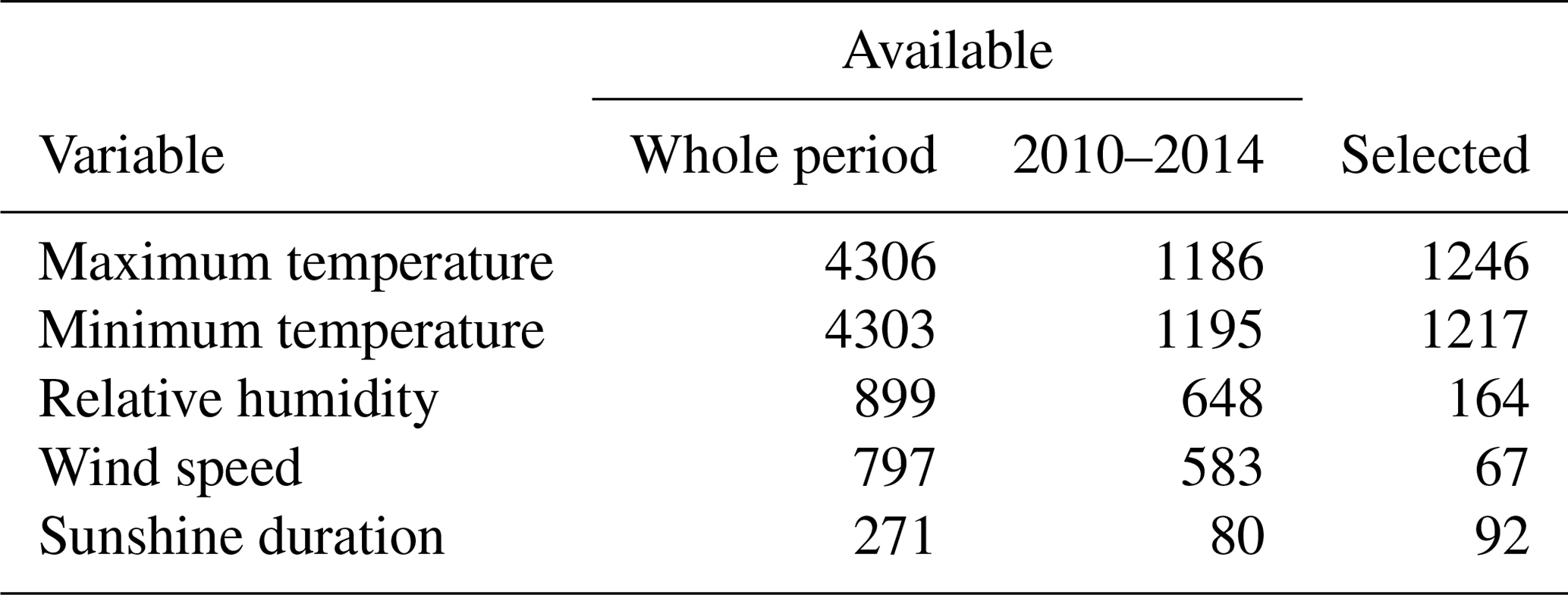
These weather stations did not collect data throughout the entire period. Figure 1 provides the number of weather observations available for each variable and each year for the 1961–2014 period. Temperature data showed the highest number of observations, always higher than 500, reaching 2000 observations available in the mid-90s, followed by a subsequent decrease. The relative humidity and wind speed showed a low number of observations during the study period. Nevertheless, in the mid-2000s, the installation of a large number of automatic weather stations (AWSs) sharply increased the availability of these two climatic variables. The sunshine duration measurements remained constant throughout the entire period.

Figure 1 Temporal evolution of the data availability.

Some geographic variables were used in the interpolation process. The digital elevation model (DEM) was obtained from the IGN (Instituto Geográfico Nacional), and other variables, such as distance to the sea, were derived from the DEM.

3 Methodology

The general scheme used to generate the ET_o database involved two main steps: (i) generation of climatic grids and (ii) estimation of ET_o (Fig. 2). The generation of the climatic grids could be divided into (a) daily quality control, (b) daily-to-weekly data conversion, (c) gap filling, (d) data selection, (e) homogenization and (f) interpolation, and all of these steps were implemented individually for each climatic variable. The estimation of ET_o consisted of the calculation of ET_o using the FAO-56 Penman–Monteith equation over the climatic grid data sources.

Figure 2 Main steps involved in generating the ET_o database. First, we interpolated each climatic variable then calculated ET_o.

On the other hand, the uncertainty in ET_o was estimated using a two-step process: (i) uncertainty estimation of the climatic grids and (ii) uncertainty propagation from the climatic grids to ET_o. The uncertainty estimation of the climatic grids estimated the uncertainty of each climatic grid after the interpolation process and considered the uncertainty related to the gap-filling process and the interpolation process. Uncertainty propagation refers to the technique used to estimate the uncertainty in ET_o values by combining the uncertainty in each climatic variable with the Jacobian of the Penman–Monteith equation.

The quality of the data were assessed by implementing an automated daily quality control in R. Daily data were tested against two types of controls: codification errors and out-of-range values. The presence of duplicate data or n consecutive days having the exact same values in different observatories were the two most relevant codification errors detected. Out-of-range values mainly detected out-of-physical-range-values and out-of-climate-range values. More details can be found in Tomas-Burguera et al. (2016). The temporal aggregation of daily data into weekly data was then executed. For all variables, weekly time series were obtained by calculating the mean value of the daily data. Weeks presenting more than 1 d without data were considered to have no data. This is an adaptation of the World Meteorological Organization (WMO) rules for monthly data (WMO, 1989).

Some comparison problems between distinct years emerged if a timescale of 7 d was used, mainly because the number of days in a year is not divisible by 7. In an attempt to combine weekly timescales to preserve comparability between years, each month was divided into 4 periods (days 1–8, 9–15, 16–22, 23–28/29/30/31). For the remainder of this discussion, the use of the word week(s) refers to this definition of a sub-monthly period.

After this step, the relative humidity data were transformed into dew point temperature (T_d) using the temperature data. Gap-filling and interpolation tests revealed that T_d was easier to work with than RH. The T_d data adjusted better to a Gaussian distribution than RH data; therefore, working with T_d data was preferable for most of the implemented steps.

3.1 Gap filling

In an effort to obtain a complete time series of distinct climate variables, a gap-filling procedure based on the estimation of missing data using nearby weather station data, designed by Beguería et al. (2019), was implemented. The standard error of the estimated data was obtained and used as a measure of the uncertainty of the process.

The selection of nearby weather stations was relevant to the process, and a selection based on three steps was implemented: (i) overlapping periods longer than 7 years, (ii) locations closer than 100 km and (iii) values of R² higher than 0.6.

The procedure used standardized values prior to gap filling in order to avoid problems related to differences in the mean values and/or variances between weather stations.

All weather stations available were used in the gap-filling process. The last step of the process involved data selection and depended on the amount of original data available. For temperature, only time series accounting for more than 25 years of the original data were used. For the rest of variables, this period was reduced to 15 years due to the low availability of long records (Fig. 3). Up to three gap-filling loops were implemented for less frequent variables (sunshine duration, dew point temperature and wind speed). Various steps in the gap-filling procedure took advantage of nonoverlapping data. This configuration was used previously to generate other databases over Spain (Gonzalez-Hidalgo et al., 2015).

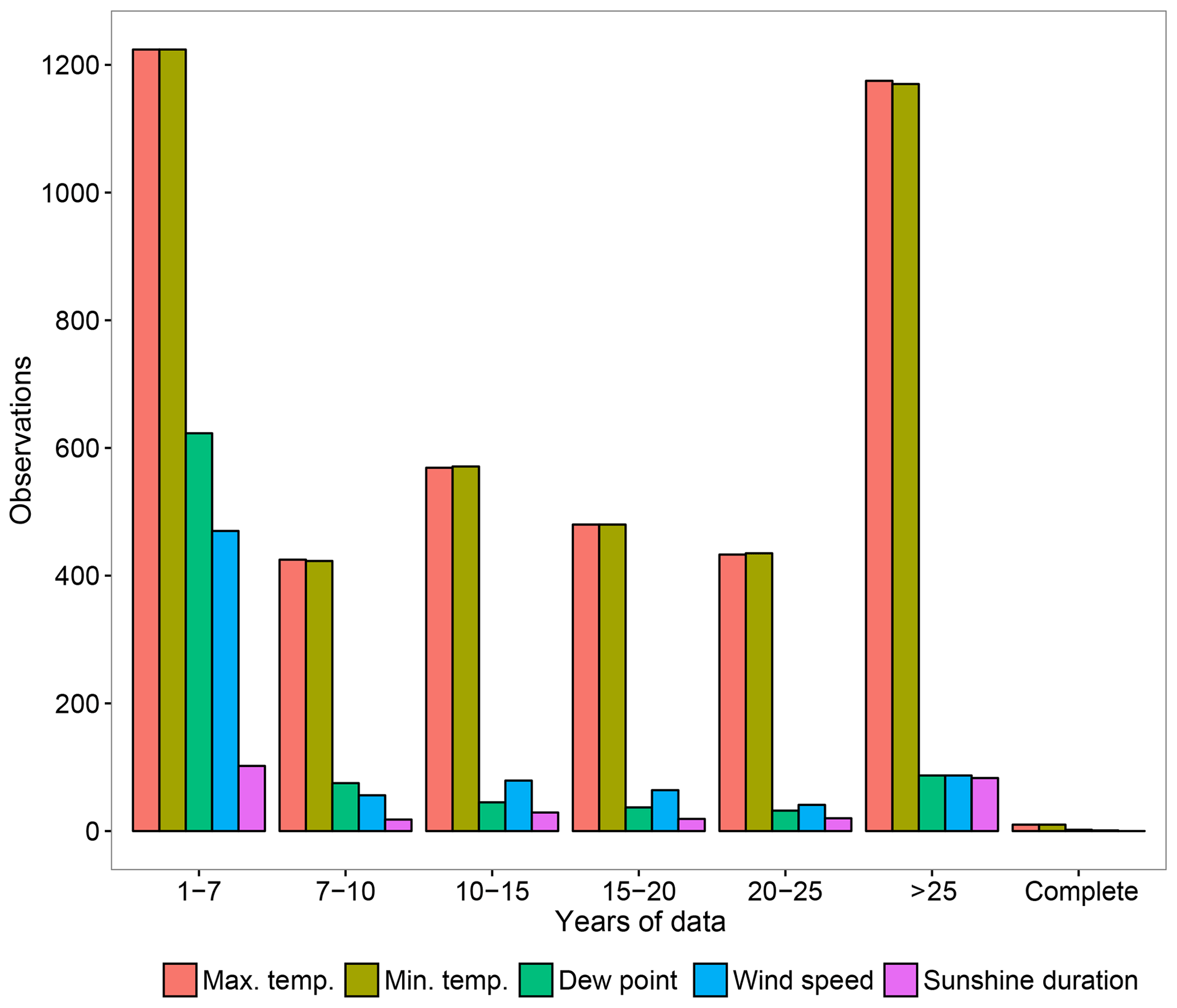
Figure 3 Number of available observations grouped by variable and by years of data available.

3.2 Homogenization

The homogeneity of the obtained time series after the gap-filling process was tested using the Standard Normal Homogeneity Test (SNHT) (Alexandersson, 1986). This method used as a basis the comparison of the time series to be homogenized, the candidate series and a reference time series. Reference time series were obtained using the same process used to obtain the gap-filling reference time series.

The test was implemented at the monthly timescale after the conversion of time series to timescales, mainly because homogeneity tests, in general, are more robust when they are used with monthly data than with sub-monthly data. Weekly homogeneous time series were obtained by transforming the monthly parameters to weekly parameters.

The climate series homogeneity was tested after gap filling to (i) detect inhomogeneities introduced by the gap-filling process and (ii) determine if the process was more reliable if the time series had no gaps.

Present observations were assumed to be standard, meaning that any inhomogeneities were corrected to adjust the values of the past to the present values.

3.3 Interpolation

Kriging is a geostatistical method widely used in climatology to generate interpolated surfaces for many variables (Aalto et al., 2013; Hofstra et al., 2008). Kriging is, in fact, a set of different methods, for example, ordinary kriging (OK) or universal kriging (UK). The main difference between OK and UK is that the former assumes the presence of a spatial constant mean, whereas the latter assumes that the spatial mean is a function that can depend on geographical factors (Cressie, 1993). The latter assumption is preferable in climatology because climate variables commonly depend on geographical factors, such as latitude, longitude, or elevation (Aalto et al., 2013). In this paper, climate grids for each variable were generated individually using UK to predict a value at each grid point for each time step.

As a first step in the interpolation process, a semi-variogram model was generated. This model was unique for each time step and each climatic variable. This process was implemented using the gstat package in R (Pebesma, 2004; Gräler et al., 2016).

Using UK data, a variance of the prediction was also obtained, and this value was used to estimate the uncertainty. One of the advantages of using the gstat package is that an uncertainty associated with observed data can be provided. We decided to use the quantification of the uncertainty obtained from the gap-filling process, which is the previous estimation process.

3.4 ET_o calculation

Predicted values of distinct climate variables were used to calculate ET_o using the FAO-PM equation (Allen et al., 1998).

$$\begin{array}{}\text{(1)}& {\mathrm{ET}}_{\mathrm{o}}={\displaystyle \frac{\mathrm{0.408}\mathrm{\Delta }(R_{\mathrm{n}}-G)+\mathit{\gamma }\left(\frac{\mathrm{900}}{T+\mathrm{273}}\right)U_{\mathrm{2}}(e_{\mathrm{s}}-e_{\mathrm{a}})}{\mathrm{\Delta }+\mathit{\gamma }(\mathrm{1}+\mathrm{0.34}{U}_{\mathrm{2}})}},\end{array}$$

where R_n is the net radiation at the crop surface (MJ m⁻² d⁻¹), G is the soil heat flux density (MJ m⁻² d⁻¹), T is the mean air temperature at 2 m (^∘C), U₂ is the wind speed at 2 m (m s⁻¹), e_s is the saturation vapor pressure (kPa), e_a is the actual vapor pressure (kPa), e_s−e_a is the saturation vapor pressure deficit (kPa), Δ is the slope of the vapor pressure curve (kPa ^∘C⁻¹) and γ is the psychrometric constant (kPa ^∘C⁻¹). The value 0.408 was used to convert from MJ m⁻² d⁻¹ units to kg m⁻² d⁻¹ (alternatively mm d⁻¹). Following the recommendations of Allen et al. (1998), we fixed G to 0, as we estimated ET_o over a time period of fewer than 10 d.

The main advantages of this equation are that it is physically based and accounts for both the radiative and aerodynamic components of evapotranspiration. The former is related to the energy available for evaporation and the latter is related to the capacity of the air to store the vapor from evapotranspiration (Azorin-Molina et al., 2015). Although the radiative component was strongly related to the solar radiation and presented a high seasonality in the study region due to its latitude, the aerodynamic component was more variable throughout the year, as it was influenced by the vapor pressure deficit as well as the wind speed. Splitting Eq. (1) into the sum of its two parts yielded the radiative component (ET_oRa) and the aerodynamic component (ET_oAe).

$$\begin{array}{}\text{(2)}& \begin{array}{rl}{\mathrm{ET}}_{\mathrm{oRa}}& ={\displaystyle \frac{\mathrm{0.408}\mathrm{\Delta }(R_{\mathrm{n}}-G)}{\mathrm{\Delta }+\mathit{\gamma }(\mathrm{1}+\mathrm{0.34}{U}_{\mathrm{2}})}}\\ {\mathrm{ET}}_{\mathrm{oAe}}& ={\displaystyle \frac{\mathit{\gamma }\left(\frac{\mathrm{900}}{T+\mathrm{273}}\right)U_{\mathrm{2}}(e_{\mathrm{s}}-e_{\mathrm{a}})}{\mathrm{\Delta }+\mathit{\gamma }(\mathrm{1}+\mathrm{0.34}{U}_{\mathrm{2}})}}\end{array}\end{array}$$

This dataset contained data describing each of the two components, ET_oRa and ET_oAe, as well as their summation, which is ET_o. A variability and trend analysis could benefit from the availability of the two components. For example, wind stilling and solar brightening have opposite effects in ET_o, but studying the two components separately facilitates the study of the impacts of each one on ET_o.

3.5 ET_o uncertainty estimation

Due to the complexity of the process involved in estimating the uncertainty in ET_o, the uncertainty in this first version of the dataset was estimated only for the final value of ET_o and not for its two components (ET_oRa and ET_oAe).

3.5.1 Uncertainty estimation in the climatic grids

Climate grid generation involves many sources of data uncertainty, including uncertainty related to the observation, the interpolation process and other sources (Haylock et al., 2008). In this paper, we assumed that uncertainty was only related to the estimation processes, i.e., gap filling and interpolation. Moreover, we considered the uncertainty of each climatic grid at each time step to be equal to the uncertainty after the interpolation process.

Uncertainty estimation over the gap-filling process was based on the number of weather observations used to estimate the missing data and the covariance between these data points. Less covariance between data was associated with more uncertainty.

The interpolation process assumed that any uncertainty was equal to the variance of the prediction, i.e., the variance of the kriging. The uncertainty estimated over the gap-filling process was propagated to the interpolation process using the gstat package in R, as the uncertainties related to the observational data used in the interpolation process were available.

3.5.2 Uncertainty propagation

The uncertainty propagation allowed us to obtain the uncertainty associated with the predicted values of ET_o (R), using the posterior variance of the climate grids and the Jacobian of the FAO-PM.

$$\begin{array}{}\text{(3)}& R={\mathbf{J}}_{{\mathrm{ET}}_{\mathrm{o}}}\mathbf{Q}({\mathbf{J}}_{{\mathrm{ET}}_{\mathrm{o}}}{)}^T,\end{array}$$

where ${\mathbf{J}}_{{\mathrm{ET}}_{\mathrm{o}}}$ is the Jacobian of ET_o and Q is the covariance matrix of the variables. For simplicity, the variables were considered to be independent, yielding a diagonal matrix with variance positions distinct from 0.

The Jacobian assumed the following form and was analytically derived.

$${\mathbf{J}}_{{\mathrm{ET}}_{\mathrm{o}}}=\left[\begin{array}{ccccc}\frac{{\mathrm{dET}}_{\mathrm{o}}}{\mathrm{d}{T}_{max}}& \frac{{\mathrm{dET}}_{\mathrm{o}}}{\mathrm{d}{T}_{min}}& \frac{{\mathrm{dET}}_{\mathrm{o}}}{\mathrm{d}{T}_{\mathrm{d}}}& \frac{{\mathrm{dET}}_{\mathrm{o}}}{\mathrm{d}W}& \frac{{\mathrm{dET}}_{\mathrm{o}}}{\mathrm{dSD}}.\end{array}\right]$$

The covariance matrix could be expressed as follows:

$$\mathbf{Q}=\left[\begin{array}{ccccc}{\mathit{\sigma }}_{T_{max}}^{\mathrm{2}}& \mathrm{0}& \mathrm{0}& \mathrm{0}& \mathrm{0}\\ \mathrm{0}& {\mathit{\sigma }}_{T_{min}}^{\mathrm{2}}& \mathrm{0}& \mathrm{0}& \mathrm{0}\\ \mathrm{0}& \mathrm{0}& {\mathit{\sigma }}_{T_{\mathrm{d}}}^{\mathrm{2}}& \mathrm{0}& \mathrm{0}\\ \mathrm{0}& \mathrm{0}& \mathrm{0}& {\mathit{\sigma }}_W^{\mathrm{2}}& \mathrm{0}\\ \mathrm{0}& \mathrm{0}& \mathrm{0}& \mathrm{0}& {\mathit{\sigma }}_{\mathrm{SD}}^{\mathrm{2}}\end{array}\right],$$

where σ² is the variance of the kriging of each of the climatic variables. In fact, as Q is a diagonal matrix, the R calculation could be rewritten as follows:

$$\begin{array}{}\text{(4)}& \begin{array}{rl}R=& {\left({\displaystyle \frac{\partial {\mathrm{ET}}_{\mathrm{o}}}{\partial T_{max}}}\right)}^{\mathrm{2}}\cdot {\mathit{\sigma }}_{T_{max}}^{\mathrm{2}}+{\left({\displaystyle \frac{\partial {\mathrm{ET}}_{\mathrm{o}}}{\partial T_{min}}}\right)}^{\mathrm{2}}\cdot {\mathit{\sigma }}_{T_{min}}^{\mathrm{2}}\\ & +{\left({\displaystyle \frac{\partial {\mathrm{ET}}_{\mathrm{o}}}{\partial T_{\mathrm{d}}}}\right)}^{\mathrm{2}}\cdot {\mathit{\sigma }}_{T_{\mathrm{d}}}^{\mathrm{2}}+{\left({\displaystyle \frac{\partial {\mathrm{ET}}_{\mathrm{o}}}{\partial W}}\right)}^{\mathrm{2}}\cdot {\mathit{\sigma }}_W^{\mathrm{2}}\\ & +{\left({\displaystyle \frac{\partial {\mathrm{ET}}_{\mathrm{o}}}{\partial \mathrm{SD}}}\right)}^{\mathrm{2}}\cdot {\mathit{\sigma }}_{\mathrm{SD}}^{\mathrm{2}}\end{array}.\end{array}$$

3.6 Using 2010–2014 data to validate the air humidity and wind speed grids

During the last part of the period (2010–2014), a high number of AWSs were installed. A sharp increase in the available RH and W data was observed during this period, compared with the data available from weather stations used to generate the original database (Table 1). The values of these observations and the values of the climate grids were compared directly to obtain the relative humidity and wind speed over the 2010–2014 period using the new stations as an independent dataset.

4 Validation

4.1 Gap filling

The performance of the gap-filling step was verified by comparing the original data and estimated data. Obviously, this comparison was only possible for periods having original data.

Table 2 lists certain statistics associated with the verification process. In general, satisfactory values of R² were achieved, with values higher than 0.9 for all variables except for the wind speed, which showed an R² of only 0.53. Evaluation of mean error (ME) and percent bias (PBIAS) showed no bias for the maximum and minimum temperature, a small negative bias for the dew point temperature (ME of −0.01 and PBIAS of −0.15) and the sunshine duration (ME of −0.01 and PBIAS of −0.23), and a positive bias for the wind speed (ME of 0.08 and PBIAS of 0.64). The ratio of the mean values and the ratio of the standard deviation showed values close to 1 for all variables. The wind speed displayed a standard deviation ratio of 1.05, meaning that the temporal variability of the gap-filling data was slightly higher than the temporal variability of the original data.

Table 2 Gap-filling statistics. Values for the following validation statistics are provided: (i) mean absolute error (MAE), (ii) coefficient of determination R², (iii) mean error (ME), (iv) percent bias (PBIAS), (v) ratio of mean values (rM) and (vi) ratio of standard deviation (rSD).

Figure 4 evaluates the possible existence of temporal differences in the performance of the gap-filling process using decadal values of R². In general, all analyzed periods showed similar performances. For wind speed, the most recent decade showed slightly higher R² values than the other decades of the period.

As the amount of original data changed over time, the amount of filled data also showed a temporal evolution. Figure 5 indicates this temporal evolution, with a higher amount of filled data during the first years of the period and a large decline over time. The amount of filled data corresponding to the maximum and minimum temperature increased again during the last several years because of a slow decline in the number of observations and the disappearance of some of the weather stations with longer records.

Figure 4 Kernel density of the gap filling R², grouped by decadal periods.

The wind speed provided the lowest amount of filled data. It was difficult to obtain highly correlated time series to fill in the gaps, which had two major effects on the process: (i) the probability of obtaining a reference time series from the neighbors was decreased and (ii) the reconstruction was poor when the reference time series could be obtained. The low correlation of the wind speed time series was a consequence of (i) the high spatial and temporal variability of this variable and (ii) the low number of observations available.

4.2 Homogenization

The percentage of data affected by the homogenization process exceeded 10 % for all variables except for the wind speed (Table 3). For all variables, the percentage of homogenized data was higher for the filled data than for the original data, indicating the importance of implementing a homogenization process after gap filling. Two factors could explain this effect: (i) because the original data were not homogenized prior to the gap filling, the presence of inhomogeneities in the original data propagated to the homogenized data and (ii) inhomogeneities may have been introduced by the gap-filling procedure.

Table 3 Percentage of data affected by inhomogeneities.

The temporal evolution of the quantity of data detected as inhomogeneous was analyzed (Fig. 5), revealing a temporal trend with maximum values at the start of the study period and minimum values at the end. The most likely explanation for this observation is the use of more recent conditions as the standard conditions.

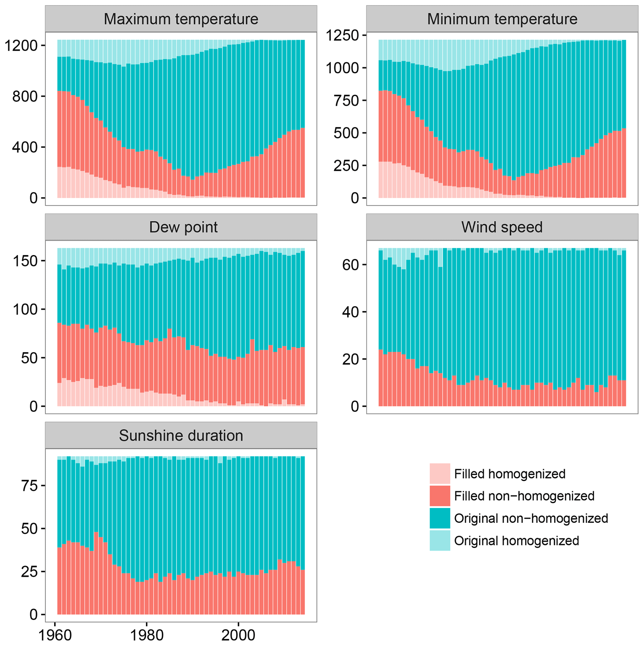
Figure 5 Temporal evolution of the number of filled data for the different climatic variables. The temporal evolution of the homogenized data is also shown.

Another effect of this assumption is the propagation of the current conditions to the past, which was evaluated by comparing the spatial mean values of the homogenized and prior-to-homogenization time series. Figure 6 highlights this effect in the implemented homogenization process. The maximum and minimum temperature, which displayed a positive trend in Spain over the study period (del Río et al., 2012; Gonzalez-Hidalgo et al., 2016), suggested that higher values occurred in the present than in the past. A positive bias was observed in the homogenized data over the first decades (1961–1970, 1971–1980 and 1981–1990). Unlike the maximum and minimum temperature, the wind speed, which displayed a negative trend (Azorin-Molina et al., 2014), was affected by a negative bias during the first decades (1961–1970, 1971–1980 and 1981–1990) of the study period.

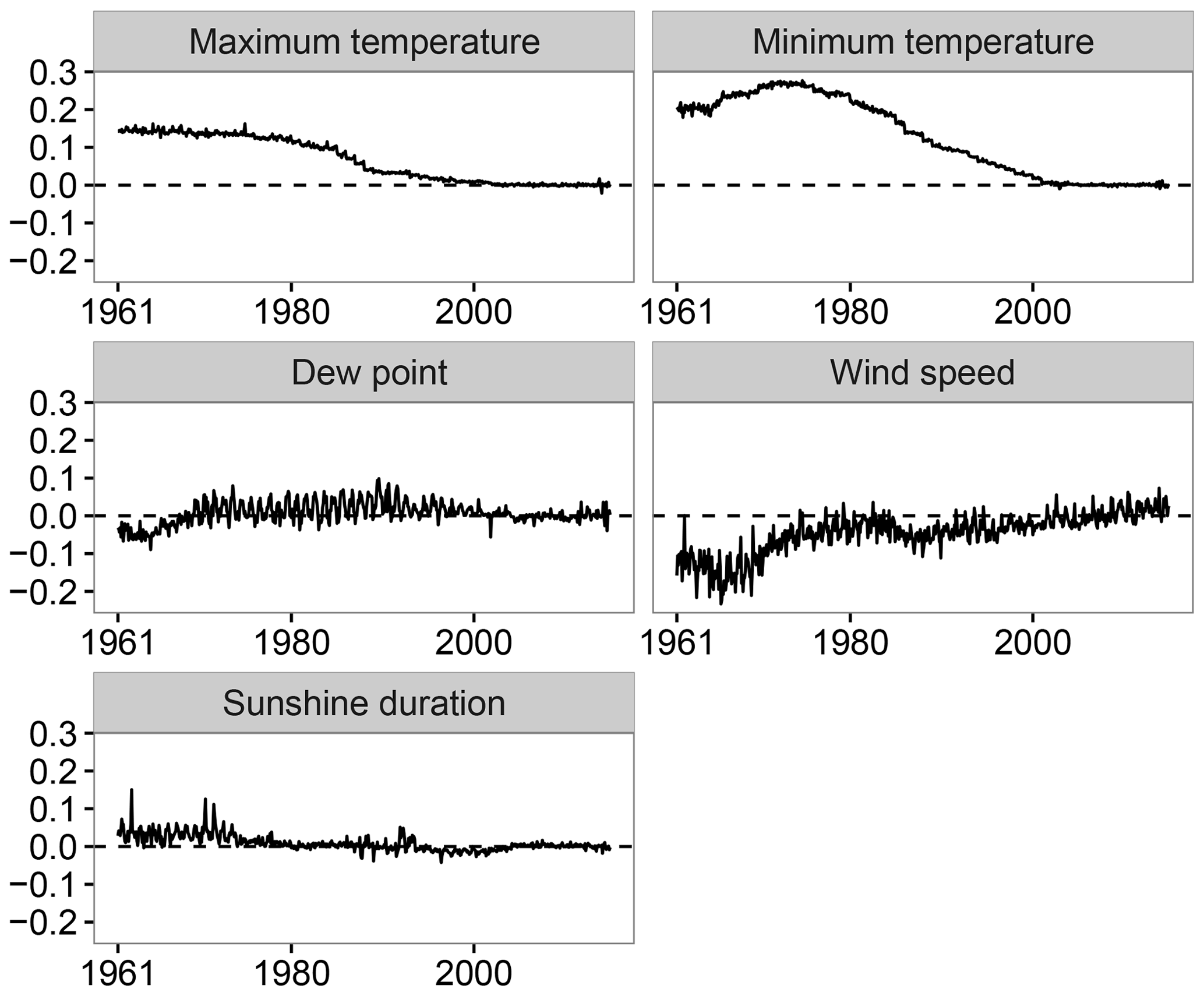
Figure 6 Temporal evolution of the differences between the mean regional values before and after homogenization.

The effect of the homogenization process on ET_o was evaluated using a similar procedure, which involved calculating the mean regional values of ET_o before and after homogenization of the climatic variables. These regional values were obtained by calculating first a mean regional value of the climatic variables, followed by calculating the ET_o using the Penman–Monteith equation.

No important differences were detected in a comparison of the two time series of ET_o (Fig. 7). This result is relevant, as it shows that the undesirable detrending introduced by the homogenization process did not affect the spatial mean values of ET_o.

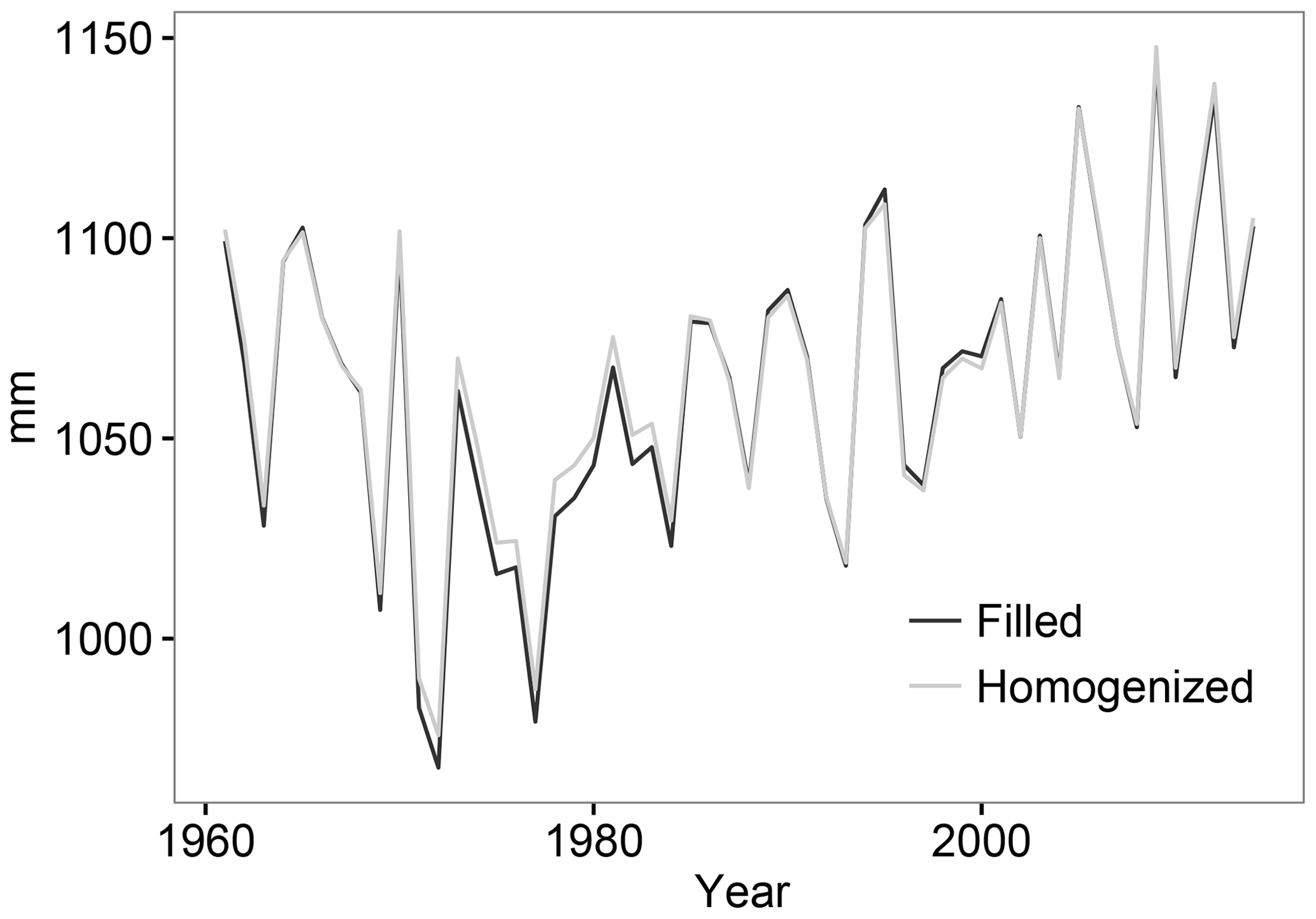
Figure 7 Temporal evolution of the mean regional values of ET_o before (filled) and after (homogenized) homogenization.

4.3 Interpolation validation

The interpolation process was validated by executing a leave-one-out cross-validation (LOO-CV) process, and validation statistics were calculated to evaluate the performance of the interpolation in predicting both the temporal variability and the spatial variability. The LOO-CV process consisted of repeating the interpolation process n times (n being the number of observations available) using each time n−1 observations and using the predicted value at the unused observatory as a way to evaluate the quality of the interpolation.

The temporal variability was evaluated by calculating the temporal statistics individually for each observatory and then computing the mean of all observatories. The spatial variability was evaluated by calculating the statistics at each time step using information comprising all observatories and then computing the mean of all time steps. The problem with the LOO-CV method is that validation could only be estimated at a given point if observations used during the interpolation process existed.

Another option for validating the interpolation process consisted of comparing the unused observational data over the 2010–2014 period (when a high number of wind speed and relative humidity observations existed) against the interpolated values.

4.3.1 Spatial and temporal validation using LOO-CV

The ability of the interpolation process to predict the spatial and the temporal variability of the climatic grids is summarized in Table 4. In general, temporal validation showed better statistics than spatial validation. All variables, except for the wind speed, showed R² values greater than 0.9 for the temporal validation and close to 0.8 for the spatial validation.

Table 4 Spatial and temporal validation of the interpolation process. Values for the following validation statistics are provided: (i) mean absolute error (MAE), (ii) coefficient of determination R², (iii) mean error (ME), (iv) percent bias (PBIAS), (v) ratio of mean values (rM) and (vi) ratio of standard deviation (rSD).

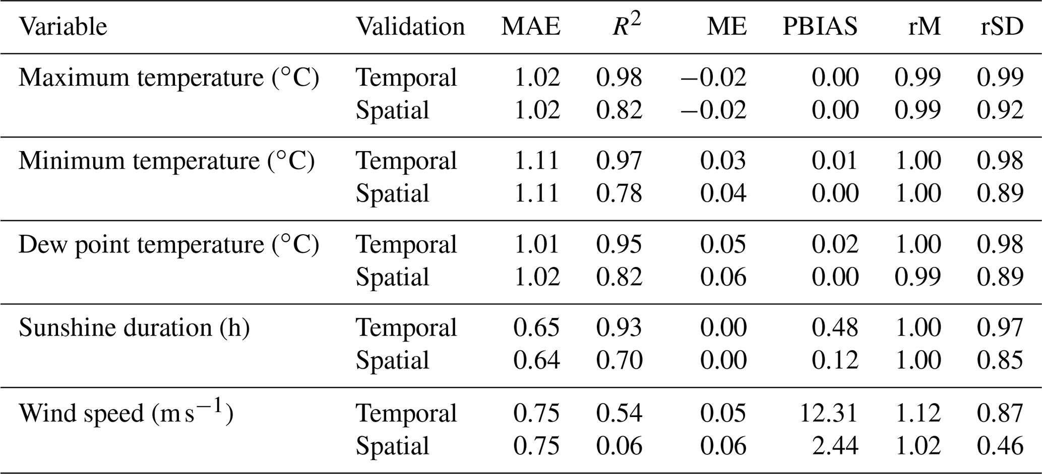
According to ME and PBIAS, the only variable that indicated the presence of bias in both validations was the wind speed, which yielded a PBIAS of 12.31 for the temporal validation.

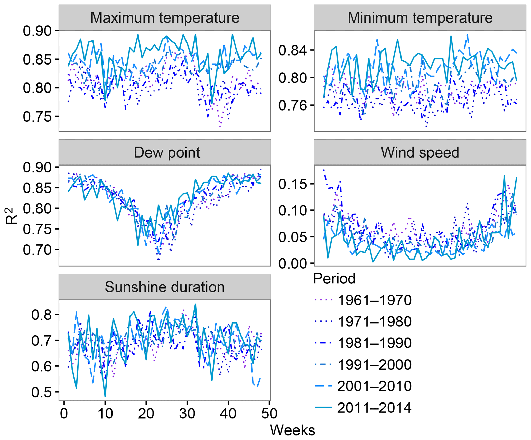
A temporal analysis of the R² values obtained from the spatial validation of the maximum and minimum temperature (Fig. 8) showed slightly better statistics (i e., closer to one) in recent decades (2001–2010 and 2011-2014). Nevertheless, the most relevant detected effect was the presence of seasonality in the R² of the dew point temperature, which indicated lower values during summer than during winter. A higher spatial variability in the air humidity in summer months due to the contrast between the high air humidity in the coastal areas and the low air humidity in the continental areas may be the source of the lower values during summer.

Figure 8 Spatial validation of the interpolation in terms of R², grouped by decadal periods.

4.3.2 The 2010–2014 validation

Validating the interpolation performance over the 2010–2014 independent time series of the wind speed and relative humidity revealed that the two most relevant detected problems were the overestimation of the wind speed during winter months in the northeastern region of the Iberian Peninsula and the overestimation of the dew point temperature in the inner region of the Iberian Peninsula during the summer months at the same time that an underestimation was detected in the maritime region. These two effects are visualized in Fig. 9, which shows the mean errors for January and July for the two variables.

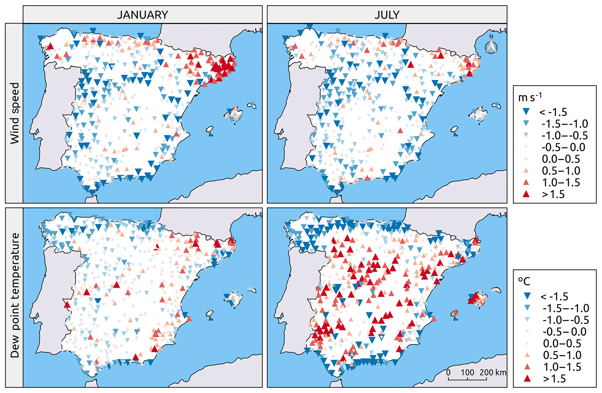
Figure 9 Spatial validation of the dew point and wind speed climatic grids using a subset of independent observations over the 2010–2014 period, in terms of the mean error.

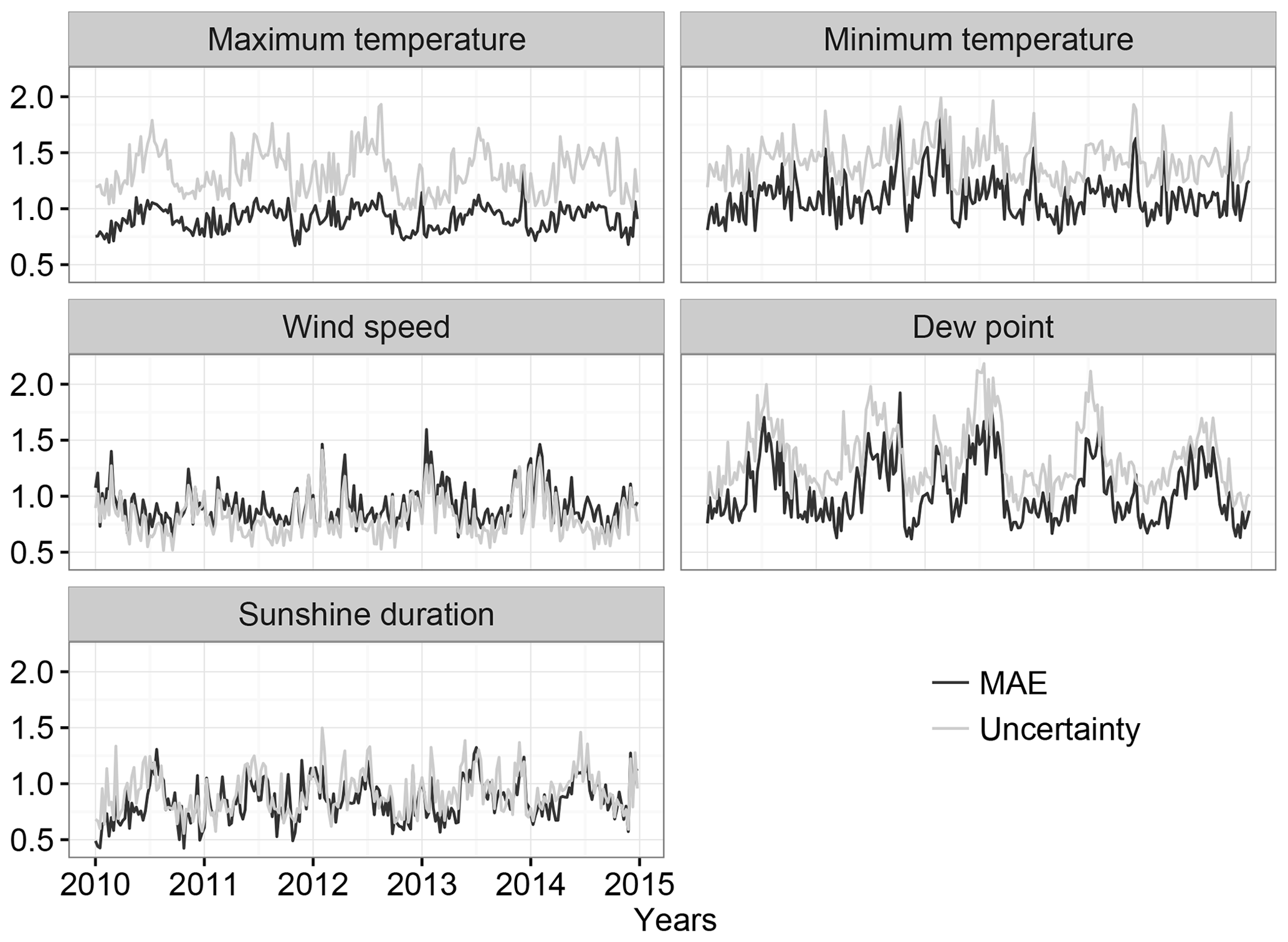
Figure 10 Temporal evolution of the MAE and uncertainty of the interpolation at a subset of independent observations over the 2010–2014 period.

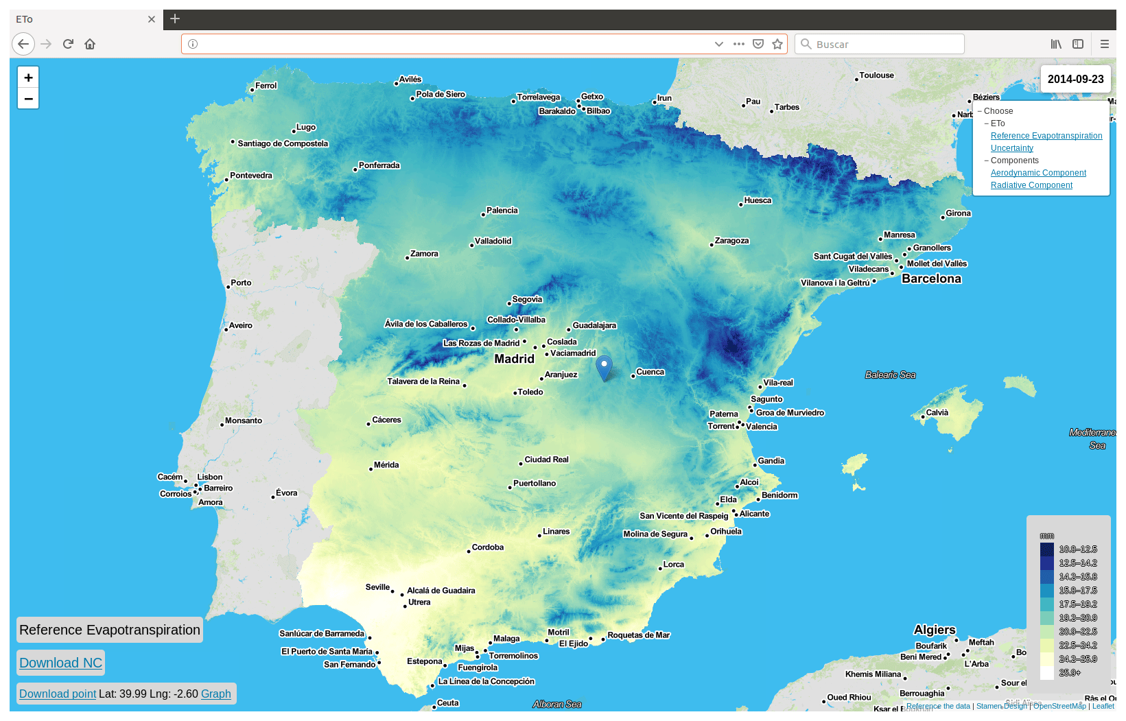
Figure 11 Example of the data visualization tool available at the following web page: http://speto.csic.es (last access: 10 December 2019).

4.3.3 Uncertainty validation

Data from the 2010–2014 period could also be used to validate the uncertainty estimation of the climatic grids. First, the mean absolute error (MAE) was calculated by comparing the independent weather station data against the climatic grid data. Then, the obtained values of the MAE were compared against the uncertainty values of the climatic grids.

The mean spatial values of the MAE and the uncertainty are represented in Fig. 10. In general, the uncertainty of the climatic grids was well estimated, especially for the wind speed and sunshine duration, as these variables showed similar values of the MAE and uncertainty. The other variables, (T_max, T_min and T_d), showed slightly higher values of uncertainty than the MAE values but always with similar temporal oscillations.

5 Data availability

The four files generated in this dataset (weekly values of reference evapotranspiration, uncertainty estimation of the weekly values of reference evapotranspiration, aerodynamic component values of the weekly reference evapotranspiration and the radiative component values of the weekly reference evapotranspiration) can be accessed and downloaded via two different sources.

From Digital CSIC, which is a long-term repository managed by the Spanish Research Council (CSIC), users can download the files in netCDF format through https://doi.org/10.20350/digitalCSIC/8615 (Tomas-Burguera et al., 2019).

The data can also be accessed at the following web page, which is a map visualization tool: http://speto.csic.es (last access: 10 December 2019). Users can visualize the data generated at different time steps, download the complete netcdf files or download a complete time series for a chosen point as a comma-separated value (csv) file. As the spatial resolution of the data is 1.1 km over continental Spain and the Balearic Islands, the total number of grid points is slightly higher than 400 000. The weekly temporal resolution yielded 2592 different weekly maps for each of the four available files.

6 Discussion and conclusions

We proposed a method for obtaining a 1961–2014 ET_o climate grid across Spain based on the Penman–Monteith equation. Whereas previous studies of ET_o and AED climatology in Spain have been developed (Azorin-Molina et al., 2015; Sanchez-Lorenzo et al., 2014; Vicente-Serrano et al., 2014), this is the first suitable ET_o database for use in climate studies covering the full study area with a high spatial resolution and over a long time period.

As the number of weather stations collecting all variables required to calculate ET_o was very low, the proposed methodology took advantage of two estimation processes: gap filling and spatial interpolation. The performances of the processes were carefully studied to detect the possible negative impacts on the generation of the ET_o database. In general, no relevant problems were detected for most of the climatic variables. The wind speed displayed the worst performance in each of the estimation processes due to its high spatial and temporal variability.

The PM-IC strategy, which consisted of interpolating climatic variables prior to calculating ET_o, was previously used to model other regions (Mardikis et al., 2005; McVicar et al., 2007) and was determined to be the best method for estimating ET_o in the event of missing data in Spain (Tomas-Burguera et al., 2017). Another strategy, known as PM-CI, calculated ET_o prior to interpolation and was also appropriate for use. The main advantage of the PM-CI over PM-IC strategy was that only one interpolation was required. The main disadvantage was that much of the available data were not used. In the case of Spain, the use of the PM-CI strategy would have restricted the calculation of ET_o to nearly 50 weather stations, which is the number of weather stations used in previous studies (Vicente-Serrano et al., 2014). On the other hand, the use of the PM-IC strategy allowed the use of more data, especially of temperature data, from more than 1000 weather stations. As 80 % of the ET_o variability was related to the variability in temperature and radiation (Mendicino and Senatore, 2013; Samani, 2000), using as many temperature observations as possible was important for ensuring the quality of the obtained results.

A comparison against an independent subset of climatic data collected over the 2010–2014 period showed the presence of a positive bias in the wind speed during winter over the northeastern region of the Iberian Peninsula. The overestimation of the wind speed in this region could be explained by the fact that a low number of observations were used in that region, and most of the observations used were located in places affected by Tramontane winds. Fortunately, the higher bias was detected in winter, when ET_o values were lower and the importance of this variable for some uses (e.g., irrigation schedule) was also lower. Two factors appeared to be relevant for wind speed estimation problems: (i) the high spatial variability of the wind speed (Luo et al., 2008) and (ii) the fact that the wind speed was not normally distributed. Both the gap-filling and interpolation processes tend to perform better when applied to normally distributed data.

These comparisons also detected some problems related to the dew point temperature values predicted during summer. An inverse bias was detected between the inland and maritime regions. During the summer months, the humidity contrast between the inland and maritime regions was high in the Iberian Peninsula, as maritime regions experienced a higher humidity due to the contributions of the sea breezes. The detected overestimation of the dew point temperature during the summer across the continental regions led to an underestimation of the vapor pressure deficit and also to an underestimation of ET_o. This effect suggested that the ET_o values were underestimated to some degree across the continental regions of Spain, whereas the maritime regions may have been affected by an overestimation.

The performance of the homogenization process was tested, and changes in the spatial mean values of the first decades were detected in some of the climatic variables. Although the maximum and minimum temperatures were affected by an increase in their spatial mean, the wind speed was affected by a decrease in the spatial mean. Due to counteracting effects, the ET_o mean spatial value was not affected by this problem.

Considering that each estimation process was affected by uncertainty, the uncertainty in ET_o after applying the two estimation processes was obtained. For simplicity, the climatic variables were considered to be independent in the final step of the uncertainty estimation, which involved the propagation of the uncertainty of each climatic variable through the Penman–Monteith equation.

Haylock et al. (2008) pointed out that the variance of the kriging, which in this paper was used to estimate the uncertainty of each climatic grid, is not a true estimation of the uncertainty; however, an evaluation of the uncertainty estimations of each variable showed a good agreement between the MAE values and the estimated uncertainty values. Unfortunately, the uncertainty of ET_o could not be verified because an independent subset of observatories that collected all variables was required to calculate ET_o but was not available.

This dataset was first developed as an input to generate, in combination with the precipitation data, grids of drought indices over the study area (Vicente-Serrano et al., 2017). Due to the relevance of ET_o and the high number of possible uses of these data, the ET_o climate grid is now being made available to other research groups. As with drought studies, in some cases the interest was focused on the combined analysis of ET_o and the precipitation data. This could be the case for hydrological studies in which the AED data can explain some of the most important processes taking place in a catchment. The combined analysis may provide better estimations of water balance and aridity indices. The present dataset covered a long period of time, thereby enabling studies of the temporal evolution of these indices.

Irrigated agriculture is another sector interested in these data, as the water balance is important both for irrigation planning and for irrigation scheduling. The development of modern irrigation systems has rendered irrigation a significant economic activity in some regions of Spain, such as the Ebro basin (Vidal-Macua et al., 2018), reinforcing the importance of the dataset in that region. More accurate models of ET_o is also useful for rainfed agriculture. Hence, the whole agricultural sector could benefit from this dataset.

This dataset could be interpreted as the first available AED climate grid across Spain, which is quite relevant to the development of spatial and temporal climatology studies that could confirm the previously detected positive trends of certain variables across the study area. This database could also be used for regional (or global) climate model assessment in the context of climate change studies.

Calculating ET_o using PM assumed a well-watered reference surface, which can differ significantly from the actual conditions present in a semiarid region, as is the case across most of our study area. A scarcity of soil moisture can decrease the air humidity and increase the air temperature compared with well-watered conditions due to the effects of the land–atmosphere continuum. Both changes, which especially affect the aerodynamic component of ET_o, may have a noticeable effect on ET_o, meaning that an overestimation can occur under semiarid conditions (Bouchet, 1963; Allen et al., 1998). Such an overestimation would be higher during the warm season when these conditions prevail. The possible overestimation due to the use of PM in a semiarid environment should be considered by potential users of this database.