the Creative Commons Attribution 4.0 License.
the Creative Commons Attribution 4.0 License.
 | 13 Jul 2018
Biophysics and vegetation cover change: a process-based evaluation framework for confronting land surface models with satellite observations
Gregory Duveiller
Giovanni Forzieri
Eddy Robertson
Goran Georgievski
Peter Lawrence
Andy Wiltshire
Philippe Ciais
Julia Pongratz
Stephen Sitch
Almut Arneth
Alessandro Cescatti
Land use and land cover change (LULCC) alter the biophysical properties of the Earth's surface. The associated changes in vegetation cover can perturb the local surface energy balance, which in turn can affect the local climate. The sign and magnitude of this change in climate depends on the specific vegetation transition, its timing and its location, as well as on the background climate. Land surface models (LSMs) can be used to simulate such land–climate interactions and study their impact in past and future climates, but their capacity to model biophysical effects accurately across the globe remain unclear due to the complexity of the phenomena. Here we present a framework to evaluate the performance of such models with respect to a dedicated dataset derived from satellite remote sensing observations. Idealized simulations from four LSMs (JULES, ORCHIDEE, JSBACH and CLM) are combined with satellite observations to analyse the changes in radiative and turbulent fluxes caused by 15 specific vegetation cover transitions across geographic, seasonal and climatic gradients. The seasonal variation in net radiation associated with land cover change is the process that models capture best, whereas LSMs perform poorly when simulating spatial and climatic gradients of variation in latent, sensible and ground heat fluxes induced by land cover transitions. We expect that this analysis will help identify model limitations and prioritize efforts in model development as well as inform where consensus between model and observations is already met, ultimately helping to improve the robustness and consistency of model simulations to better inform land-based mitigation and adaptation policies. The dataset consisting of both harmonized model simulation and remote sensing estimations is available at https://doi.org/10.5281/zenodo.1182145.
- Article
(4430 KB) - Full-text XML
-
Supplement
(7214 KB) - BibTeX
- EndNote


Terrestrial vegetation regulates land–climate interactions through both biogeochemical and biogeophysical mechanisms. The role of vegetation from the biogeochemical side relies on its capacity to act either as a carbon sink or a carbon source (Le Quéré et al., 2016). Changes in land cover, which are dominated by forest area loss, have a pronounced effect on climate by reducing the terrestrial carbon stocks (Canadell and Raupach, 2008). However, land cover also controls both radiative and non-radiative biophysical surface properties of vegetation that influence the water, momentum and energy budgets (Bonan, 2008). Land use and land cover change (LULCC) alters these biophysical properties and in turn affects the local climate through changes in the surface energy balance (Anderson et al., 2011; Bonan, 2008; Davin and de Noblet-Ducoudré, 2010; Lee et al., 2011; Mahmood et al., 2014; Pielke et al., 2011). For instance, a vegetation cover transition from forest to grassland typically causes an increase in albedo (because grasses are generally brighter than trees and in cold climates grasses have a more homogeneous snow cover during the cold season; see Betts and Ball, 1997; Jackson et al., 2008; Loranty et al., 2014), but also a decrease in summer evapotranspiration (because grasses have lower aerodynamic conductance, see Bonan, 2008, and they typically have shallower roots and thus cannot access water in deeper soil horizons, e.g. Canadell et al., 1996; Fan et al., 2017; Oliveira et al., 2005). The result of competing biophysical processes on the surface energy balance varies spatially and temporally and can lead to warming or cooling depending on the specific vegetation change and on the background climate (e.g. presence of snow or soil moisture) (Pitman et al., 2011). In some cases, the associated changes in biophysical properties may offset the intended biogeochemical effects of land-based mitigation (Betts, 2000). Yet, policies tackling climate mitigation through land management focus only on biogeochemical mechanisms and neglect their biophysical consequences.
Recent advances have demonstrated that satellite remote sensing observations can provide valuable diagnostics of the effect of vegetation cover change on their biophysical properties (Alkama and Cescatti, 2016; Duveiller et al., 2018b; Forzieri et al., 2017; Li et al., 2015; Zhao and Jackson, 2014). Biophysical surface properties, such as albedo (Schaaf et al., 2002) and land surface temperature (Wan, 2008), are typically more accessible to remote sensing instruments than biogeochemical properties like carbon stocks and fluxes. The latent heat flux of the land can also be estimated from remote sensing observations using data-driven models (McCabe et al., 2016; Miralles et al., 2011; Mu et al., 2007), while the residual sensible and ground heat fluxes can be obtained from a combination of such datasets by imposing the closure of the surface energy balance (Duveiller et al., 2018b; Forzieri et al., 2017). To exploit such datasets for analysing the biophysical effects of LULCC, two different approaches are typically adopted. The first focuses on places where vegetation cover has changed over a period of time and compares the situation before and after this event, taking care in controlling for the effects of inter-annual climatic variability over a local window (e.g. Silvério et al., 2015; Alkama and Cescatti, 2016). The second approach relies on a space-for-time substitution that isolates the potential impact of a land cover transition by comparing neighbouring areas with similar environmental conditions but contrasting vegetation (e.g. Zhao and Jackson 2014; Li et al., 2015; Peng et al., 2014; Duveiller et al., 2018b). Both appear to yield similar results (Li et al., 2016), but the space-for-time approach allows the exploration of more transitions and over a larger spatial extent since it is not limited to places where actual change has occurred (Duveiller et al., 2018b).
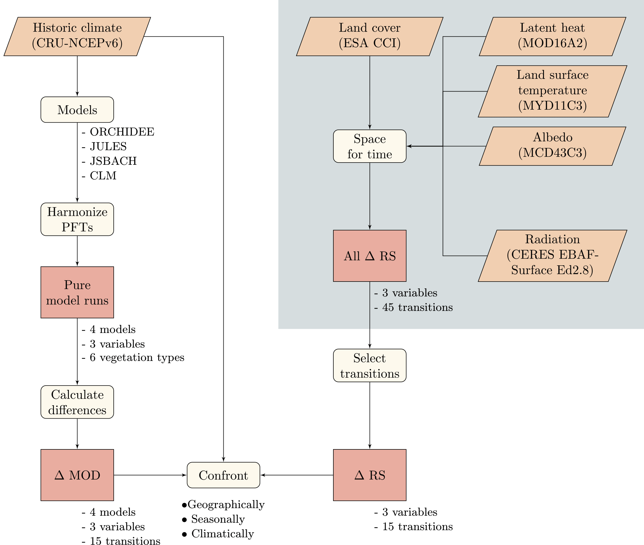
Figure 1Flowchart resuming the processing steps undertaken for the present study. The part in the grey box corresponds to work done in a previous study (Duveiller et al., 2018b).
The biophysical consequences of LULCC are known to depend on the background climate (Pitman et al., 2011; Winckler et al., 2017b), which in turn varies with climate change (IPCC, 2014). To better anticipate these changes it is necessary to predict these biophysical effects with robust model frameworks. Land surface models (LSMs) are used to represent terrestrial processes within Earth system models, in which they simulate both the carbon cycle and land-atmosphere fluxes of energy, water and momentum. Initiatives like the Land-Use and Climate, Identification of Robust Impacts (LUCID) project (de Noblet-Ducoudré et al., 2012; Pitman et al., 2009) have attempted to evaluate the capacity of LSMs to represent biophysical effects of LULCC by inter-comparing several simulations of past LULCC and showing large discrepancies amongst models, especially in separating between turbulent fluxes. Such inter-comparison exercises should also continue within broader initiatives such as the Land Use Model Inter-comparison Project (LUMIP) contribution to the Coupled Model Intercomparison Project Phase 6 (CMIP6) (Lawrence et al., 2016). However, there is a lack of model evaluation against observation-driven datasets, in which the spatial, temporal and climatic patterns can be evaluated at finer scale. Confrontation with observations could considerably contribute towards improving the robustness and consistency of models, but requires special attention to ensure simulations and observations are comparable regarding how vegetation cover is implemented and how biophysical processes are represented.
This study presents a framework for process-oriented model evaluation specifically tailored towards analysing how local biophysical effects of vegetation cover change are represented in LSMs. Simulations from four major LSMs are confronted with satellite remote sensing observations across geographic, seasonal and climatic dimensions for a range of vegetation transitions and for different components of the surface energy balance. The main objectives of this study are to create a harmonized multi-dimensional dataset, to illustrate its content and to demonstrate its utility by evaluating the agreement amongst models and against satellite observations.
Isolating the effect of vegetation cover change from both model simulations and observations in order to make them comparable requires a series of dedicated processing steps. To assist the reader in following the methodology developed in this work, Fig. 1 summarizes the main steps in a synthetic flowchart.
2.1 Remote sensing estimations
The observation part of the analysis is based on satellite remote sensing observations to assess the effects of vegetation on the surface energy balance for different vegetation cover types (Duveiller et al., 2018a). This remote sensing dataset (RS dataset for short) consists of spatially and seasonally explicit estimates of changes in surface properties following specific vegetation transitions. These surface properties are albedo, land surface temperature (LST) and evapotranspiration (ET), obtained from the respective MODIS products MCD43C3 (Schaaf et al., 2002), MYD11C3 (Wan, 2008) and MOD16A2 (Mu et al., 2011). The changes in these variables are calculated at the original scale of the product 0.05∘, but the dataset is provided at a spatial resolution of 1∘, with each cell representing the mean changes occurring at the finer scale of 0.05∘. This coarser spatial resolution is necessary for a specific step to ingest CERES EBAF surface radiation data (Kato et al., 2013) in the processing chain, but is also ideal to align the dataset with the simulations of LSMs. The data represent a multi-annual average year with a monthly temporal resolution. This synthetic year is constructed from the median values for a given month over the period 2008–2012 for every 0.05∘ pixel. The original land cover map used to build this dataset is the ESA CCI land cover map for 2010 (ESA, 2017), but with a simplified reclassification of land cover types into major vegetation classes according to the International Geosphere-Biosphere Programme (IGBP) classification scheme. A total of 45 distinct vegetation transitions are provided in the RS dataset. Although these are referred to as vegetation transitions, the information does not come from observations over transient vegetation changes, but rather from paired observations of distinct vegetation cover types at the same location. As a result, values for a given pair are only available where there is sufficient spatial abundance, or co-occurrence, of both vegetation types. For more details on the dataset and how it was produced, readers may refer to Duveiller et al. (2018a).
The surface property variables from the RS dataset are net radiation (Rn), latent heat flux (LE), and the sum of sensible and ground heat flux (H + G). Sensible and ground heat fluxes have to be considered together because they cannot be directly retrieved from satellites and are computed as a residual flux from the closure of the surface energy balance. However, it can be considered that H + G is dominated by H since the ground heat values are generally much smaller and can be neglected at annual scale. In this study net radiation is considered positive when the flux goes from the atmosphere to the ground, while latent, sensible and ground heat fluxes are positive when they exit from the surface to the atmosphere.
2.2 Land surface model simulations
To simulate the biophysical effects of local vegetation transitions that are comparable to the RS dataset, we need to run LSMs forced by a realistic climate and with idealized vegetation distributions. The four models evaluated here are ORCHIDEE (Krinner et al., 2005), JULES (Best et al., 2011; Clark et al., 2011), JSBACHv3.1 (Reick et al., 2013) and CLM4.5 (Oleson et al., 2013). The forcing consists of historic climate data from CRU-NCEP v6, and observationally derived global atmospheric CO2 concentration (Le Quéré et al., 2015). Models were spun up for steady state in biomass pools and leaf area index (LAI) and then forced with transient CRU-NCEP v6 reconstructed climate and CO2 from 1950 or earlier, and up until 2014. To obtain values of the surface variables of interest (Rn, LE and H + G) that are coherent with those of the RS dataset, the median monthly values of these fluxes from 2008 until 2012 was calculated.
Models differ in how they represent the surface energy balance per plant functional type (PFT) at the sub-grid level. Not all models can calculate heat fluxes per PFT within a grid cell, and thus some need to resort to flux aggregation at grid cell level to derive resulting variables such as temperature. To overcome this problem and isolate the effect of vegetation cover change on the surface energy budget, simulations are made in which the entire grid cell is covered by a single PFT. Separate simulations are run for each PFT of every model, in which the entire surface of the Earth is covered by a single PFT. The effect of a change in PFT can then be retrieved by subtracting values of biophysical fluxes between the two corresponding simulations. Since there is no feedback between the vegetation and the climate in this set-up, having such homogeneous distributions of vegetation across vast geographic extents does not generate climate biases outside of the grid cell.
2.3 Harmonizing vegetation classes
The models differ in how they represent vegetation using different PFTs, each with their own parametrization. To facilitate the harmonization with the IGBP vegetation classes in the remote sensing dataset, only 6 broad vegetation classes are considered: evergreen broadleaf trees (EvgTr), deciduous broadleaf trees (DecTr), needleleaf trees (NedTr), shrubs (Shrub), grasses (Grass) and crops (Crops). A total of 15 transitions (from paired comparisons of PFTs) are thus available and can also be used to represent inverse transitions (e.g. ΔLE for DecTr to Crops is equal to −ΔLE for Crops to DecTr). To obtain these broad vegetation classes from the RS dataset, the IGBP classes of evergreen and deciduous needleleaf forest (ENF and DNF, respectively) were merged into NedTr, whereas classes not represented by models or mixed classes such as woody savannas (SAV), mixed forests (MF) and wetlands (WET) have been omitted. The other three classes (Shrub, Grass and Crops) can be directly assigned with their corresponding classes in the scheme used in the RS dataset (SHR, GRA and CRO).
Table 1Summary of how the specific plant functional types (PFTs) of the different land surface models (LSMs) are mapped into the six broad vegetation classes used in this study. Model-specific nomenclature of PFT is used in italics.
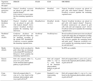
The spatial merging of different PFTs into single simulation layers requires assignment from ancillary maps indicated by the following superscripts: a Köppen–Geiger classification (Kottek et al., 2006) to distinguish arid, tropical, temperate and boreal climate zones; b default PFT distribution of JSBACH including dominant photosynthetic pathways (Knorr and Heimann, 2001).
The harmonization of the different modelled PFTs to these 6 broad classes required the use of some decision rules that are summarized in Table 1. PFTs whose differences relate to their climatic regime (such as “Tropical broadleaf deciduous” and “Temperate broadleaf deciduous” in ORCHIDEE) are geographically separated and can be aggregated into a single global PFT. The spatial representation of the climate zones is taken from the revisited Köppen–Geiger classification product (Kottek et al., 2006). A similar approach is adopted to keep all needleleaf tree PFTs in a single layer, as the deciduous needleleaf trees are predominantly located in a well-defined geographic area in Siberia without a strong overlap with evergreen needleleaf trees. For grasses and crops, LSMs typically make a separation between C3 and C4 systems for carbon fixation, which is not currently feasible to detect from remote sensing observations (and thus is absent in the RS dataset). For the two classes, Grass and Crops, the decision rule adopted is to assign the dominant photosynthetic pathway (C3 or C4) within a grid cell to the entire grid cell. Since different models may have a different default PFT distribution map, the PFT distribution of JSBACH (based on work by Knorr and Heimann, 2001) is selected here as reference and used for the harmonization of the other models as well. An exception to this rule is applied for JULES, which represents crops as grasses. In this case, to maximize information content the Crops class is assigned exclusively with the C3 grass PFT and the Grass class contains only the C4 grass PFT. There are some further model-specific details in the harmonization procedure. For CLM, the Crops simulation is composed exclusively of the generic C3 crop. Even if some LSMs can simulate some crop managements options, such as irrigation, this has been switched off to maximize inter-comparability amongst model runs. Regarding trees, JULES does not distinguish PFTs based on phenology, considering only the difference between broadleaf and needleleaf trees. The EvgTr and DecTr simulations will therefore be identical in JULES. Shrubs are simulated as a PFT by all models except for ORCHIDEE, for which the Shrub class remains empty.
As mentioned previously, the RS dataset can only provide reliable estimations where the vegetation types of interest locally co-exist. Although the models could theoretically simulate the vegetation even where is does not naturally occur, the harmonized dataset presented here only includes simulated values over the areas where the RS data are available.

Figure 2Inter-comparison of how the land surface models and remote sensing (RS) estimate a change in latent heat flux (LE) for the vegetation transition from evergreen broadleaf trees to crops (Crops – EvgTr). We summarize the data within three different comparison spaces to illustrate (a) the spatial variability, representing the annual mean for each pixel; (b) the seasonal variability; and (b) the variability in climate space, represented by mean annual temperature and annually cumulated precipitation.
2.4 Protocol to evaluate agreement
The harmonized dataset is presented and analysed along three different bi-dimensional spaces. The first is geographic space, in which mean annual values per pixel are obtained by averaging all monthly observations. The second is labelled seasonal space, in which averages are made along latitudinal bands for each month, illustrating the seasonal course of the variables, such as in Hovmöller diagrams (Hovmöller, 1949). The third is climatic space, in which variables are analysed along temperature and precipitation gradients. The climatic axes of this space are mean annual temperature and annually cumulated precipitation for the period 2008–2012 based on the CRU TS4.00 climate data (Harris et al., 2014). The rationale behind using these spaces is to encourage more process-based model evaluation by ensuring that the agreement or disagreement between models and observations is coherent spatially, seasonally and climatically.
In this context of quantifying the biophysical effects of vegetation cover change, neither the satellite-derived estimations nor any of the model simulations can pretend to be an absolute reference, as all of them have some level of assumptions and uncertainties. While observation-driven datasets are usually taken as a reference over model simulations, in some cases the latter can also serve to evaluate the quality of the former (Massonnet et al., 2016). In order to evaluate the agreement without setting a single product as a reference, we measure agreement based on a metric that has the property of being symmetric. This means the value of the metric remains numerically unchanged whether it is applied to products X and Y, or if these are inverted. This is not the case when using a coefficient of determination R2 from a standard regression of Y on X, which differs from that of a regression of X on Y. Beyond being symmetric, the index of agreement λ that we use is also dimensionless, bounded (between 0 for no agreement to 1 for perfect agreement) and easy to compute (Duveiller et al., 2016). Furthermore, its interpretation is relatively intuitive for practitioners since its value is the same as that of the familiar correlation coefficient r when there are no additive or multiplicative bias contributing to the disagreement between X and Y. When there are biases, its value reduces proportionately to this bias. For two sets, X and Y, each containing n values, the index is defined as follows:
where μ and σ represent the mean and standard deviation, respectively. κ is a term set to zero if the correlation between X and Y is positive, and otherwise set as follows:
Besides this index of agreement, the analysis also uses the correlation coefficient r and the mean absolute bias B as defined by the following formulas:
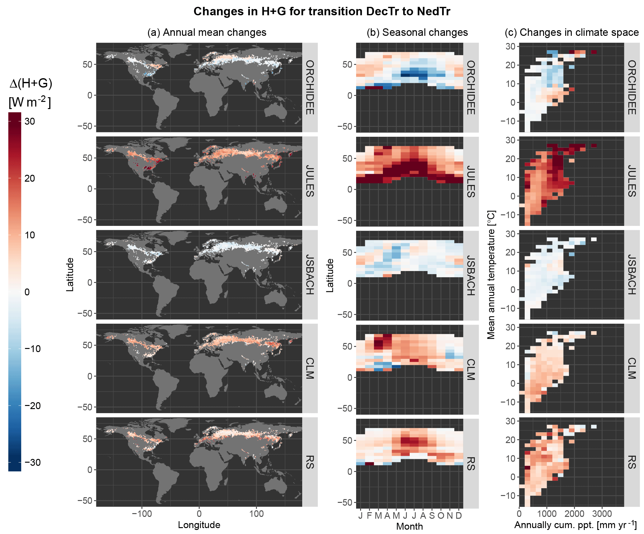
Figure 3Same as Fig. 2 for a change in the residual flux of the energy balance composed of both sensible heat and ground heat fluxes (H + G) for the vegetation transition from deciduous broadleaf trees to needleleaf trees (DecTr – NedTr).
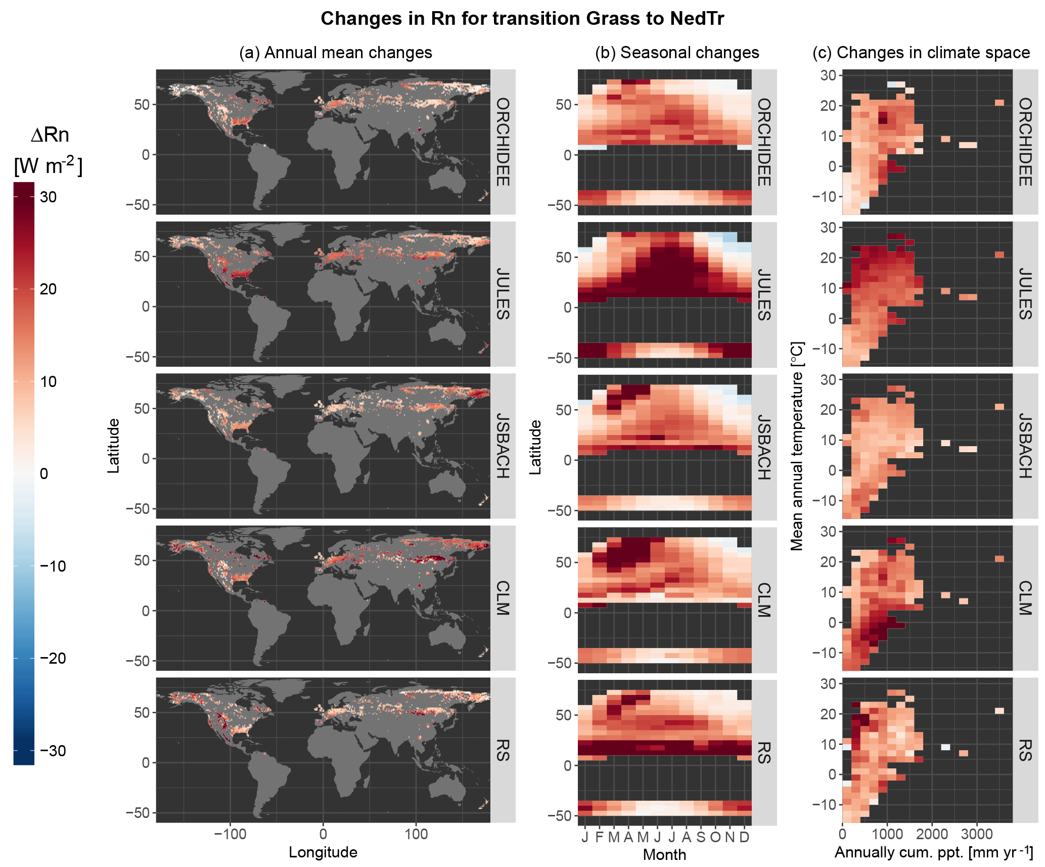
Figure 4Same as Fig. 2 for a change in the net radiative flux (Rn) for the vegetation transition from grasses to needleleaf trees (Grass – NedTr).
Due to its high dimensionality, it is challenging to illustrate exhaustively all the facets of information represented in the dataset. Therefore, this section starts by describing a selection of cases of how different products portray changes in geographic, seasonal and climatic space of a given variable following a specific vegetation cover transition.
The first case, shown in Fig. 2, consists of changes in LE resulting from the conversion of evergreen broadleaf trees to crops (EvgTr to Crops) corresponding to a common land cover change associated with tropical deforestation. It is clear from this figure that not all models reproduce the expected effects of tropical deforestation (i.e. a reduction in LE due to crops having shallower roots and thus less access to water for transpiration) that are seen in the RS dataset. JSBACH and CLM see an increase in mean annual LE following deforestation in large parts of the world. ORCHIDEE and JULES generally predict the sign correctly, a reduction of LE, but for JULES the behaviour in the seasonal and climatic space shows contrasting patterns to those of RS, while those of JSBACH might be more in line despite the constant bias of this model. Please note that in this and similar figures presented in this work, data for a given transition are only available for areas where there is a local co-occurrence of the two vegetation types according to the land cover distribution used in the RS dataset.
The second case, displayed in Fig. 3, concerns changes in H + G following the conversion of broadleaf deciduous to needleleaf trees (DecTr to NedTr). This transition can represent for instance changes in planted forest species, such as what occurred for most of the past 250 years in Europe (Naudts et al., 2016). According to the RS dataset, this change is associated with a general increase in H + G, particularly in the summer period and across all latitudes (at least those in which there is a joint presence of DecTr and NedTr, and thus a higher likelihood that this conversion occurs). ORCHIDEE and JSBACH do not capture the sign of change in H + G dynamic, sometimes showing a reduction in H + G that is quite large for ORCHIDEE in the summertime and in warmer climates. CLM and JULES show more consistent patterns with RS. However, JULES overestimates the magnitude of change, especially in warmer climates, while CLM simulates a higher rise in H + G in spring in northern mid-latitudes to high latitudes that is not present in the observations.
The effect on net radiation caused by vegetation change from grasses to needleleaf trees (Grass to NedTr) is the third case, illustrated in Fig. 4. This transition reflects the effect of a northward expansion of the boreal forests into tundra, which is expected to happen as the temperatures in the higher latitudes increase. It also represents land abandonment and reforestation in the mid-latitudes. The general direction of change is captured by all models, showing how transforming grasslands to forests leads to an increase in net radiation, mostly due to the increase in shortwave radiation absorbed by the darker canopy. However, the geographic, seasonal and climatic patterns differ from observations and vary across the models. Seasonally, the RS dataset illustrates the strong snow effect on albedo in northern latitudes in spring, when the radiation load increases substantially as the days become longer while snow cover remains, thus amplifying the albedo differences between snow-covered grasses and darker evergreen trees. The higher increases in Rn that are present in the RS observations along the mountain ranges in North America are only captured by JULES. The magnitude of the spring albedo effect for this transition is slightly underestimated in ORCHIDEE and overestimated in JSBACH and CLM, although for CLM it appears to extend more in time and latitude than what is reported in the RS dataset. While these discrepancies might be due more to misrepresentation of snow-related processes within the models than to misrepresentation of vegetation, it remains a good example of a process-based model evaluation, since it focuses on the comprehensive biophysical effect of the process of vegetation cover change.
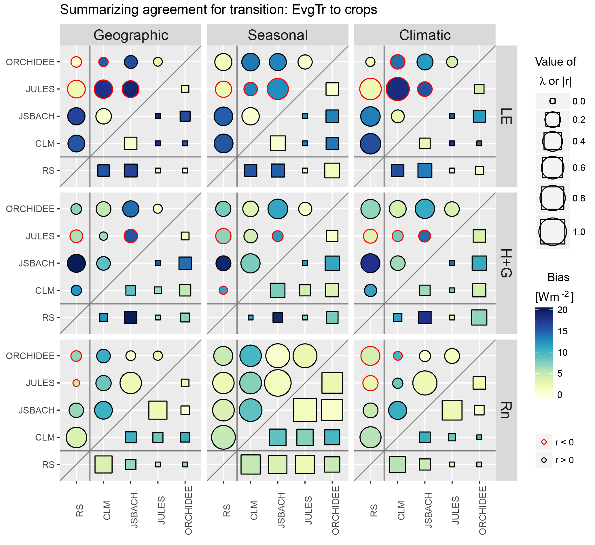
Figure 5Summary of the agreement between land surface models amongst themselves and with the remote sensing estimations for the vegetation transition from evergreen broadleaf trees to crops (Crops – EvgTr). The agreement is measured using the index of agreement λ (size of the squares), the Pearson correlation coefficient r (size of the circles, red border indicates negative correlation) and the absolute bias (colour of the symbols). The data used to calculate these metrics are the values previously averaged in bins according to the spatial, seasonal and climatic analysis spaces shown in Fig. 2. Hence, these metrics relate only to areas where both vegetation types locally co-exist in reality. The fluxes represented are net radiation (Rn), latent heat flux (LE), and the combination of the sensible and ground heat fluxes (H + G).
For any vegetation transition, the similarities and discrepancies, both amongst models and with the RS dataset, can be summarized synthetically in a single diagram for all fluxes and for the three spaces under investigation (geographic, seasonal and climatic). Figure 5 shows such a diagram for the case of the tropical deforestation transition EvgTr to Crops, the same transition which is represented in Fig. 2. Every panel in Fig. 5 provides an inter-comparison of the pair-wise agreement between products either with the index λ, using squares in the lower right triangle of the panel, or with the correlation coefficient, r, using circles in the upper left triangle. Whilst the sizes of the symbols represent the relative value of the metric, the colour provides the value of the mean absolute bias. For two products X and Y, all metrics (λ, r and B) are calculated using the respective equations with the aggregated values over the three reasoning spaces, i.e. the binned values in geographic, seasonal and climatic space, such as those represented in Fig. 2. Generally Rn is better represented across the board, especially the seasonal patterns, and LE tends to suffer larger biases. The agreement amongst the models can be also gauged by comparing the size of the symbols within the triangles of Fig. 5. Analogous plots to those in Fig. 5 are available for all 15 transitions in the Supplement.
To provide a general overview for all transitions, Fig. 6 shows the agreement for each model with the RS dataset for all three fluxes averaged over geographic, seasonal and climatic space. The transitions are ordered according to the magnitude of gross transitions that have occurred in the recent past between 2000 and 2015 according to the annual ESA CCI annual land cover maps (ESA, 2017), with EvgTr to Crops being the largest. Generally, the agreement in geographic space is very poor, followed by occasional agreement in climatic space, and then more frequent agreement regarding the seasonal cycle. Net radiation is the variable that models simulate best, particularly the seasonal patterns, while H + G come second and LE comes third. Overall, the transition in which there is highest agreement between models and RS across all variables and spaces is DecTr to Crops, while the one with least agreement is Grass to Crops.
No model stands out as having consistently better performance than the others. Models differ in which transitions they simulate best. JULES performs best for NedTr to Grass, CLM for EvgTr to Crops, and both JSBACH and ORCHIDEE for DecTr to Crops. When looking at each variable across transitions and facets, the models showing highest mean agreement for LE, H + G and Rn are JULES, CLM and JULES respectively. Disregarding the situations when agreement is very poor, rare are the cases when all models similarly agree with RS, i.e. when all colours in a single box of Fig. 6 have similar colours. Those that stand out always involve Rn and are seasonal agreement for Grass to DecTr and both seasonal and climatic agreement for DecTr to Crops. There are also cases in which a single model stands out as having much higher agreement than all the others, such as CLM for the spatial agreement of Rn for EvgTr to Crops, JULES for the seasonal agreement of Rn for NedTr to DecTr, JSBACH for climatic agreement of H + G for NedTr to Shrub and ORCHIDEE for climatic agreement of H + G for NedTr to Crops.
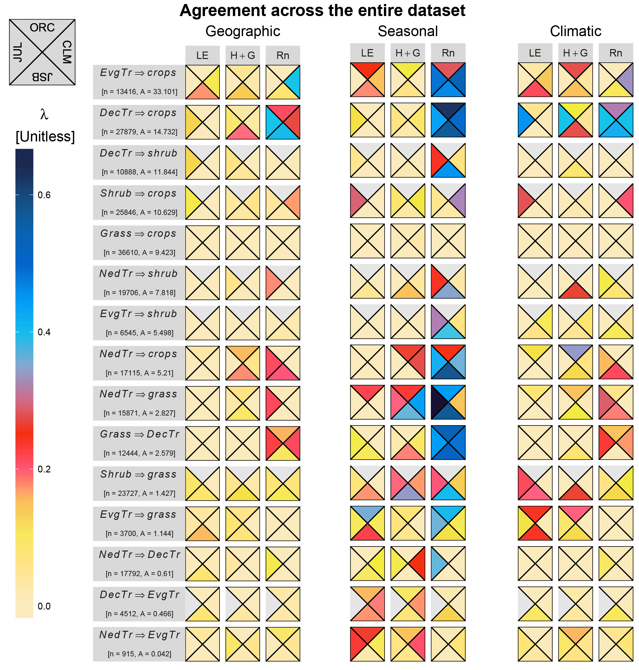
Figure 6Summary of the agreement between models and remote sensing for all fluxes and all transitions in each of three facets of analysis: spatial, seasonal and climatic. The position of each triangle represents one of the four land surface models as shown in the top corner: ORCHIDEE (ORC), the Community Land Model (CLM), JSBACH (JSB) and JULES (JUL). The fluxes represented are net radiation (Rn), latent heat flux (LE), and the combination of the sensible and ground heat fluxes (H + G). The colour of the triangle represents the value of the index of agreement λ. Below each transition label, the number n provides the total number of original individual spatio-temporal records used to calculate each metric. The order of the transitions (from top to bottom) corresponds to the order of gross changes that have occurred between 2000 and 2015 according the ESA CCI land cover maps, which is provided below each transition label in megahectares (Mha).
A final synoptic summary is provided in Fig. 7 that encompasses all transition and all fluxes and separates the total agreement in the recurrent three spaces: geographic, seasonal and climatic. A further division is made by distinguishing between the mean agreement amongst models (analogously to the triangle of values mentioned for Fig. 5) and the mean model agreement with remote sensing. The more salient feature is that models seem to agree most over Europe. Inter-model agreement is also high over northern America, but with the notable exception of the southeast of the United States. Inter-model agreement is also higher in drier and colder areas. However, for many of these areas models do not agree with RS. Western Canada and southern Australia appear as the places where there is the strongest agreement with RS, while the tropics show decisively lower agreement. The higher agreement amongst models in northern latitudes is maintained across the seasons, but the agreement with RS is only high in spring, probably due to the capacity of some models to catch the snow-induced albedo changes when trees are replaced by shrubs or grasses. The overall agreement in climate space indicates how for warm climates, models agree amongst themselves less in the more humid conditions, while there is generally a large disagreement with RS for all conditions. In colder climates, inter-model agreement is high but agreement with RS is higher for wetter conditions.
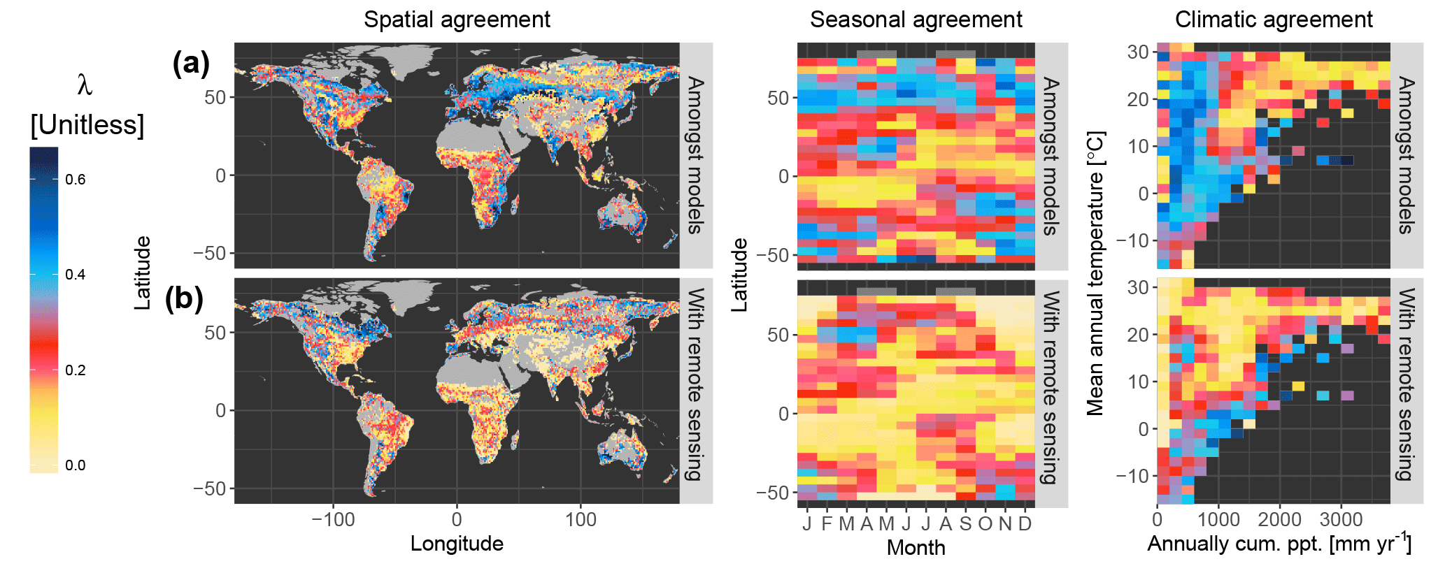
Figure 7Agreement amongst models and between models and remote sensing for all transitions and all fluxes together. The agreement amongst models (a) is calculated as the mean of all λ values calculated for each model pairs, while the agreement with remote sensing (b) is the mean values of λ for each model with respect to the remote sensing dataset.
This model-evaluation framework specifically targeting the biophysical effects of LULCC is unique in that it brings model simulations and observation-driven estimates together. By focusing on a model set-up with prescribed homogeneous vegetation types within grid cells, the biophysical impacts of specific LULCC transitions within the models can be recombined to match RS observations without requiring a complex disaggregation of the energy balance fluxes per sub-grid PFT. The resulting harmonized dataset should be of interest for a range of stakeholders. Model developers will find it useful to assess how their model performs with respect to other models and to an observational benchmark, which in turn can serve to identify areas across geographic, seasonal and climate space where model development efforts should be prioritized. Developers of LSMs that are not included in this study can follow the protocol and use the dataset to evaluate the resulting model performance. Model users can use the dataset and the analysis to choose the LSM that performs best over their areas of interest. For people making decisions based on conclusions derived from model outputs, the dataset and the evaluation can provide a welcome overview of model performance across space, time and climate zones, along with an overall an idea of the current level of uncertainty associated with using these tools for estimating the biophysical impacts of LULCC.
The overall picture of the general benchmarking exercise of model performances is not encouraging. For various vegetation transitions, models do not even agree amongst themselves on the magnitude nor the sign of the change. The study confirms with observational data what previous analyses had reported based on model inter-comparisons regarding how models have more difficulties to simulate turbulent fluxes than radiative ones (de Noblet-Ducoudré et al., 2012), despite that the former have been shown to drive the local temperature response to land cover and management (Bright et al., 2017). As can be expected, the seasonal patterns observed in the RS dataset are better simulated than climatic or spatial patterns. Models are especially poor in capturing the spatial patterns, arguably because LSMs typically use the same parameterization for a given PFT across the globe, thereby disregarding the spatial variability of traits that can naturally occur, which in turn is sampled by the observation-driven estimates. In this sense, some model improvement could come by adopting the concept of optical functional types, based on traits detectable by remote sensing (Ustin and Gamon, 2010).
Models also tend to agree more amongst themselves than with observations. This may stem from similarities in the construction of models and their underlying assumptions. Europe may come out as a place of higher inter-model agreement because vegetation models were based heavily on information on temperate ecosystems, resulting in a better representation of temperature deciduous systems than drought-deciduous systems (Morales et al., 2005). Data for other ecosystems have only become available in more recent decades. Inter-model agreement, and to a lesser extent RS-model agreement, is also higher in the areas where flux measurements from eddy-covariance towers, frequently used for carbon cycle calibration, are denser (Schimel et al., 2015). This converges towards an evident conclusion that strengthening the observational base is still essential to ensure the quality of model results. As discussed in Duveiller et al. (2018b), the RS dataset also has shortcomings, and these may partly explain discrepancies with respect to model simulations. A valid criticism is that the RS dataset relies on an evapotranspiration product (Mu et al., 2011) that has been shown to underperform compared to other satellite-driven products both at local (Michel et al., 2016) and at global scales (Miralles et al., 2016). However, this was the only available product at the sufficiently fine spatial resolution of 0.05∘, and despite the underperformance, ancillary analyses in Duveiller et al. (2018a, b) suggest that the product quality is sufficient for the purpose of studying local differences.
Some caveats regarding the specific model set-up need to be highlighted. The first relates to the spatial scale at which processes are represented. The use of homogeneous PFTs across grid cells successfully isolates the effect of a total vegetation cover change within an LSM grid, but this has a natural trade-off: intrinsically heterogeneous ecosystems, such as savanna systems and taiga, could not be evaluated as these are represented by models using a mixture of tree and grass PFTs. A dedicated evaluation could be done in a more sophisticated version of this work using the savanna class transitions in the RS dataset (which was not used here), but would require the use of the same prescribed mixture of trees and grasses for all models. Such an exercise would probably reveal strong changes in biophysical effects linked to canopy roughness. Another option could be to do the entire exercise on LAI, which can integrate this heterogeneity, comparing changes in modelled LAI with LAI estimated from satellite remote sensing. A related caveat in the current set-up linked to mixed systems is that a within-grid cell bias may result from the mismatch between climate and vegetation. In an all-forest simulation over a grid cell subjected to the real climate observed over a savanna, the trees may be more stressed than if they were mixed with low-evaporative grasses. Therefore, transitions of forests to grasses reported in this dataset may be overestimating the reduction of processes such as evapotranspiration over savanna regions. Overall, these issues illustrate how increasing the spatial resolution of the model simulations to better match that of observations should improve their inter-comparisons. This would result both from a better characterization of vegetation heterogeneity, but also from enabling LSMs to better resolve local climate variability and the resulting biophysical effects of LULCC.
Another particularity of the model set-up employed here is that only the local first-order biophysical effects of LULCC are explored. Non-local effects related to LULCC occurring elsewhere, as explored by modelling exercises such as Winckler et al. (2017a), are not considered here because they cannot be directly estimated by remote sensing diagnostics. Given that the analysis is also based on uncoupled LSMs runs, there are no possible feedbacks of the vegetation cover change on global climate, nor are there any local atmospheric feedbacks. Considering second-order effects stemming from the bi-directional land–climate interactions would require using LSMs coupled with a general circulation model within an Earth system model in which some cells are affected by LULCC, but this is beyond the scope of the present work.
The inter-comparison exercise presented here can be extended and improved. Doing so could further address other limitations of the current set-up, such as the fact that only a single source of meteorological forcing data is used to run the model simulations. Such datasets, based on climate reanalysis, can be particularly prone to errors and uncertainties in data-poor regions. Initiatives such as LUMIP (Lawrence et al., 2016) could use the present framework to run LSMs with different forcing datasets and evaluate how the simulated biophysical impacts of LULCC are sensitive to the quality of the input data. Another criticism of the inter-comparison is the mismatch between model runs, which do not explicitly include the effects of land management, and the RS dataset, which intrinsically does, simply because these are present in the observations. The biophysical impacts of land management changes have been shown to be as important as the effects of land cover change (Luyssaert et al., 2014), and could thus further account for the discrepancies between models and observations. The exercise could thus be extended with runs that include management for the models which can effectively simulate it, and it could also evaluate the improvement based on the RS benchmark. Finally, the exercise could be improved by extending the observational part to an ensemble of RS datasets. The input biophysical variables used to construct the RS dataset, namely albedo, land surface temperature and evapotranspiration, could be derived from different satellite instruments and based on other, ideally better algorithms. Ultimately, the RS dataset could be based on products from geostationary satellites to be able to study the diurnal patterns of biophysical effects of LULCC and how these are represented in the models.
The dataset consisting of both harmonized model simulation and remote sensing estimations is freely available in Zenodo: https://doi.org/10.5281/zenodo.1182145 (Duveiller et al., 2018c).
This paper presents a process-oriented model evaluation framework for biophysical effects of vegetation cover change. A harmonized multi-dimensional dataset has been generated including dedicated simulations from four major LSMs along with observation-driven estimations based on satellite imagery. The analysis of these data along geographic, seasonal and climate dimensions results in an overview of model performance that can serve to highlight hotspots of agreement and disagreement both amongst models and with respect to an observational benchmark. The overall capacity of current LSMs to represent biophysical effects of LULCC is low. The seasonal cycle of radiative fluxes is the process that models capture best, whilst performance drops considerably when considering spatial and climatic gradients for all fluxes. We anticipate that the dataset will serve to identify specific model shortcomings with respect to observations and to other models, but also to highlight where models can be trusted more and where model development should be prioritized. This should in turn contribute to the larger goal to develop and inform land-based mitigation and adaptation policies that account for both biogeochemical and biophysical vegetation impacts on climate. Improving the robustness and consistency of land-surface models is essential to develop and inform land-based mitigation and adaptation policies that account for both biogeochemical and biophysical vegetation impacts on climate.
The supplement related to this article is available online at: https://doi.org/10.5194/essd-10-1265-2018-supplement.
GD, AC and SS conceived the study. ER, WL, GG and PL did the model runs, which GF harmonized together. GD did all the analyses and wrote the paper with contribution of all the authors.
The authors declare that they have no conflict of interest.
The study was funded by the FP7 LUC4C project (grant no.
603542)
Edited by: David
Carlson
Reviewed by: Wim Thiery and one anonymous referee
Alkama, R. and Cescatti, A.: Biophysical climate impacts of recent changes in global forest cover, Science, 351, 600–604, https://doi.org/10.1126/science.aac8083, 2016.
Anderson, R. G., Canadell, J. G., Randerson, J. T., Jackson, R. B., Hungate, B. a, Baldocchi, D. D., Ban-Weiss, G. a, Bonan, G. B., Caldeira, K., Cao, L., Diffenbaugh, N. S., Gurney, K. R., Kueppers, L. M., Law, B. E., Luyssaert, S. and O'Halloran, T. L.: Biophysical considerations in forestry for climate protection, Front. Ecol. Environ., 9,174–182, https://doi.org/10.1890/090179, 2011.
Best, M. J., Pryor, M., Clark, D. B., Rooney, G. G., Essery, R. L. H., Ménard, C. B., Edwards, J. M., Hendry, M. A., Porson, A., Gedney, N., Mercado, L. M., Sitch, S., Blyth, E., Boucher, O., Cox, P. M., Grimmond, C. S. B., and Harding, R. J.: The Joint UK Land Environment Simulator (JULES), model description – Part 1: Energy and water fluxes, Geosci. Model Dev., 4, 677–699, https://doi.org/10.5194/gmd-4-677-2011, 2011.
Betts, A. K. and Ball, J. H.: Albedo over the boreal forest, J. Geophys. Res.-Atmos., 102, 28901–28909, https://doi.org/10.1029/96JD03876, 1997.
Betts, R.: Offset of the potential carbon sink from boreal forestation by decreases in surface albedo, Nature, 408, 187–90, https://doi.org/10.1038/35041545, 2000.
Bonan, G. B.: Forests and climate change: forcings, feedbacks, and the climate benefits of forests, Science, 320, 1444–1449, https://doi.org/10.1126/science.1155121, 2008.
Bright, R. M., Davin, E., O'Halloran, T., Pongratz, J., Zhao, K., and Cescatti, A.: Local temperature response to land cover and management change driven by non-radiative processes, Nat. Clim. Change, 7, 296–302, https://doi.org/10.1038/nclimate3250, 2017.
Canadell, J., Jackson, R. B., Ehleringer, J. B., Mooney, H. A., Sala, O. E. and Schulze, E.-D.: Maximum rooting depth of vegetation types at the global scale, Oecologia, 108, 583–595, https://doi.org/10.1007/BF00329030, 1996.
Canadell, J. G. and Raupach, M. R.: Managing Forests for Climate Change Mitigation, Science, 320, 1456–1457, https://doi.org/10.1126/science.1155458, 2008.
Clark, D. B., Mercado, L. M., Sitch, S., Jones, C. D., Gedney, N., Best, M. J., Pryor, M., Rooney, G. G., Essery, R. L. H., Blyth, E., Boucher, O., Harding, R. J., Huntingford, C., and Cox, P. M.: The Joint UK Land Environment Simulator (JULES), model description – Part 2: Carbon fluxes and vegetation dynamics, Geosci. Model Dev., 4, 701–722, https://doi.org/10.5194/gmd-4-701-2011, 2011.
Davin, E. L. and de Noblet-Ducoudré, N.: Climatic Impact of Global-Scale Deforestation: Radiative versus Nonradiative Processes, J. Climate, 23, 97–112, https://doi.org/10.1175/2009JCLI3102.1, 2010.
Duveiller, G., Fasbender, D., and Meroni, M.: Revisiting the concept of a symmetric index of agreement for continuous datasets, Sci. Rep.-UK, 6, 19401, https://doi.org/10.1038/srep19401, 2016.
Duveiller, G., Hooker, J., and Cescatti, A.: A dataset mapping the potential biophysical effects of vegetation cover change, Sci. Data, 5, 180014, https://doi.org/10.1038/sdata.2018.14, 2018a.
Duveiller, G., Hooker, J., and Cescatti, A.: The mark of vegetation change on Earth's surface energy balance, Nat. Commun., 9, 679, https://doi.org/10.1038/s41467-017-02810, 2018b.
Duveiller, G., Forzieri, G., Robertson, E., Li, W., Georgievski, G., Lawrence, P., Wiltshire, A., Ciais, Ph., Pongratz, J., Sitch, S., Arneth, A., and Cescatti, A.: Biophysical effects of vegetation cover change from satellite and models, Zenodo, https://doi.org/10.5281/zenodo.1182145, 2018c.
ESA: Land Cover CCI Product User Guide Version 2, available at: http://maps.elie.ucl.ac.be/CCI/viewer/download/ESACCI-LC-Ph2-PUGv2_2.0.pdf (last access: 9 July 2018), 2017.
Fan, Y., Miguez-Macho, G., Jobbágy, E. G., Jackson, R. B., and Otero-Casal, C.: Hydrologic regulation of plant rooting depth, P. Natl. Acad. Sci. USA, 114, 10572–10577, https://doi.org/10.1073/pnas.1712381114, 2017.
Forzieri, G., Alkama, R., Miralles, D. G., and Cescatti, A.: Satellites reveal contrasting responses of regional climate to the widespread greening of Earth, Science, 356, 1180–1184, https://doi.org/10.1126/science.aal1727, 2017.
Harris, I., Jones, P. D., Osborn, T. J., and Lister, D. H.: Updated high-resolution grids of monthly climatic observations – the CRU TS3.10 Dataset, Int. J. Climatol., 34, 623–642, https://doi.org/10.1002/joc.3711, 2014.
Hovmöller, E.: The Trough-and-Ridge diagram, Tellus, 1, 62–66, https://doi.org/10.3402/tellusa.v1i2.8498, 1949.
IPCC: Climate Change 2014: Impacts, Adaptation, and Vulnerability, Part A: Global and Sectoral Aspects, Contribution of Working Group II to the Fifth Assessment Report of the Intergovernmental Panel on Climate Change, edited by: Field, C. B., Barros, V. R., Dokken, D. J., Mach, K. J., Mastrandrea, M. D., Bilir, T. E., Chatterjee, M., Ebi, K. L., Estrada, Y. O., Genova, R. C., Girma, B., Kissel, E. S., Levy, A. N., MacCracken, S., Mastrandrea, P. R., and White, L. L., Cambridge University Press, Cambridge, UK, New York, NY, USA, 2014.
Jackson, R. B., Randerson, J. T., Canadell, J. G., Anderson, R. G., Avissar, R., Baldocchi, D. D., Bonan, G. B., Caldeira, K., Diffenbaugh, N. S., Field, C. B., Hungate, B. A., Jobbágy, E. G., Kueppers, L. M., Nosetto, M. D., and Pataki, D. E.: Protecting climate with forests, Environ. Res. Lett., 3, 044006, https://doi.org/10.1088/1748-9326/3/4/044006, 2008.
Kato, S., Loeb, N. G., Rose, F. G., Doelling, D. R., Rutan, D. A., Caldwell, T. E., Yu, L., and Weller, R. A.: Surface Irradiances Consistent with CERES-Derived Top-of-Atmosphere Shortwave and Longwave Irradiances, J. Climate, 26, 2719–2740, https://doi.org/10.1175/JCLI-D-12-00436.1, 2013.
Knorr, W. and Heimann, M.: Uncertainties in global terrestrial biosphere modeling: 1. {A} comprehensive sensitivity analysis with a new photosynthesis and energy balance scheme, Global Biogeochem. Cy., 15, 207–225, https://doi.org/10.1029/1998GB001059, 2001.
Kottek, M., Grieser, J., Beck, C., Rudolf, B., and Rubel, F.: World Map of the Köppen-Geiger climate classification updated, Meteorol. Z., 15, 259–263, https://doi.org/10.1127/0941-2948/2006/0130, 2006.
Krinner, G., Viovy, N., de Noblet-Ducoudré, N., Ogée, J., Polcher, J., Friedlingstein, P., Ciais, P., Sitch, S., and Prentice, I. C.: A dynamic global vegetation model for studies of the coupled atmosphere-biosphere system, Global Biogeochem. Cy., 19, 1–33, https://doi.org/10.1029/2003GB002199, 2005.
Lawrence, D. M., Hurtt, G. C., Arneth, A., Brovkin, V., Calvin, K. V., Jones, A. D., Jones, C. D., Lawrence, P. J., de Noblet-Ducoudré, N., Pongratz, J., Seneviratne, S. I., and Shevliakova, E.: The Land Use Model Intercomparison Project (LUMIP) contribution to CMIP6: rationale and experimental design, Geosci. Model Dev., 9, 2973–2998, https://doi.org/10.5194/gmd-9-2973-2016, 2016.
Lee, X., Goulden, M. L., Hollinger, D. Y., Barr, A., Black, T. A., Bohrer, G., Bracho, R., Drake, B., Goldstein, A., Gu, L., Katul, G., Kolb, T., Law, B. E., Margolis, H., Meyers, T., Monson, R., Munger, W., Oren, R., Paw, U. K. T., Richardson, A. D., Schmid, H. P., Staebler, R., Wofsy, S., and Zhao, L.: Observed increase in local cooling effect of deforestation at higher latitudes, Nature, 479, 384–387, https://doi.org/10.1038/nature10588, 2011.
Le Quéré, C., Moriarty, R., Andrew, R. M., Canadell, J. G., Sitch, S., Korsbakken, J. I., Friedlingstein, P., Peters, G. P., Andres, R. J., Boden, T. A., Houghton, R. A., House, J. I., Keeling, R. F., Tans, P., Arneth, A., Bakker, D. C. E., Barbero, L., Bopp, L., Chang, J., Chevallier, F., Chini, L. P., Ciais, P., Fader, M., Feely, R. A., Gkritzalis, T., Harris, I., Hauck, J., Ilyina, T., Jain, A. K., Kato, E., Kitidis, V., Klein Goldewijk, K., Koven, C., Landschützer, P., Lauvset, S. K., Lefèvre, N., Lenton, A., Lima, I. D., Metzl, N., Millero, F., Munro, D. R., Murata, A., Nabel, J. E. M. S., Nakaoka, S., Nojiri, Y., O'Brien, K., Olsen, A., Ono, T., Pérez, F. F., Pfeil, B., Pierrot, D., Poulter, B., Rehder, G., Rödenbeck, C., Saito, S., Schuster, U., Schwinger, J., Séférian, R., Steinhoff, T., Stocker, B. D., Sutton, A. J., Takahashi, T., Tilbrook, B., van der Laan-Luijkx, I. T., van der Werf, G. R., van Heuven, S., Vandemark, D., Viovy, N., Wiltshire, A., Zaehle, S., and Zeng, N.: Global Carbon Budget 2015, Earth Syst. Sci. Data, 7, 349–396, https://doi.org/10.5194/essd-7-349-2015, 2015.
Le Quéré, C., Andrew, R. M., Canadell, J. G., Sitch, S., Korsbakken, J. I., Peters, G. P., Manning, A. C., Boden, T. A., Tans, P. P., Houghton, R. A., Keeling, R. F., Alin, S., Andrews, O. D., Anthoni, P., Barbero, L., Bopp, L., Chevallier, F., Chini, L. P., Ciais, P., Currie, K., Delire, C., Doney, S. C., Friedlingstein, P., Gkritzalis, T., Harris, I., Hauck, J., Haverd, V., Hoppema, M., Klein Goldewijk, K., Jain, A. K., Kato, E., Körtzinger, A., Landschützer, P., Lefèvre, N., Lenton, A., Lienert, S., Lombardozzi, D., Melton, J. R., Metzl, N., Millero, F., Monteiro, P. M. S., Munro, D. R., Nabel, J. E. M. S., Nakaoka, S.-I., O'Brien, K., Olsen, A., Omar, A. M., Ono, T., Pierrot, D., Poulter, B., Rödenbeck, C., Salisbury, J., Schuster, U., Schwinger, J., Séférian, R., Skjelvan, I., Stocker, B. D., Sutton, A. J., Takahashi, T., Tian, H., Tilbrook, B., van der Laan-Luijkx, I. T., van der Werf, G. R., Viovy, N., Walker, A. P., Wiltshire, A. J., and Zaehle, S.: Global Carbon Budget 2016, Earth Syst. Sci. Data, 8, 605–649, https://doi.org/10.5194/essd-8-605-2016, 2016.
Li, Y., Zhao, M., Motesharrei, S., Mu, Q., Kalnay, E., and Li, S.: Local cooling and warming effects of forests based on satellite observations, Nat. Commun., 6, 6603, https://doi.org/10.1038/ncomms7603, 2015.
Li, Y., Zhao, M., Mildrexler, D. J., Motesharrei, S., Mu, Q., Kalnay, E., Zhao, F., Li, S., and Wang, K.: Potential and Actual impacts of deforestation and afforestation on land surface temperature, J. Geophys. Res.-Atmos., 121, 14372–14386, https://doi.org/10.1002/2016JD024969, 2016.
Loranty, M. M., Berner, L. T., Goetz, S. J., Jin, Y., and Randerson, J. T.: Vegetation controls on northern high latitude snow-albedo feedback: observations and CMIP5 model simulations, Glob. Change Biol., 20, 594–606, https://doi.org/10.1111/gcb.12391, 2014.
Luyssaert, S., Jammet, M., Stoy, P. C., Estel, S., Pongratz, J., Ceschia, E., Churkina, G., Don, A., Erb, K., Ferlicoq, M., Gielen, B., Grünwald, T., Houghton, R. A., Klumpp, K., Knohl, A., Kolb, T., Kuemmerle, T., Laurila, T., Lohila, A., Loustau, D., McGrath, M. J., Meyfroidt, P., Moors, E. J., Naudts, K., Novick, K., Otto, J., Pilegaard, K., Pio, C. A., Rambal, S., Rebmann, C., Ryder, J., Suyker, A. E., Varlagin, A., Wattenbach, M., and Dolman, A. J.: Land management and land-cover change have impacts of similar magnitude on surface temperature, Nat. Clim. Change, 4, 389–393, https://doi.org/10.1038/nclimate2196, 2014.
Mahmood, R., Pielke, R. A., Hubbard, K. G., Niyogi, D., Dirmeyer, P. A., McAlpine, C., Carleton, A. M., Hale, R., Gameda, S., Beltrán-Przekurat, A., Baker, B., McNider, R., Legates, D. R., Shepherd, M., Du, J., Blanken, P. D., Frauenfeld, O. W., Nair, U. S., and Fall, S.: Land cover changes and their biogeophysical effects on climate, Int. J. Climatol., 34, 929–953, https://doi.org/10.1002/joc.3736, 2014.
Massonnet, F., Bellprat, O., Guemas, V., and Doblas-Reyes, F. J.: Using climate models to estimate the quality of global observational data sets, Science, 354, 452–455, https://doi.org/10.1126/science.aaf6369, 2016.
McCabe, M. F., Ershadi, A., Jimenez, C., Miralles, D. G., Michel, D., and Wood, E. F.: The GEWEX LandFlux project: evaluation of model evaporation using tower-based and globally gridded forcing data, Geosci. Model Dev., 9, 283–305, https://doi.org/10.5194/gmd-9-283-2016, 2016.
Michel, D., Jiménez, C., Miralles, D. G., Jung, M., Hirschi, M., Ershadi, A., Martens, B., McCabe, M. F., Fisher, J. B., Mu, Q., Seneviratne, S. I., Wood, E. F., and Fernández-Prieto, D.: The WACMOS-ET project – Part 1: Tower-scale evaluation of four remote-sensing-based evapotranspiration algorithms, Hydrol. Earth Syst. Sci., 20, 803–822, https://doi.org/10.5194/hess-20-803-2016, 2016.
Miralles, D. G., Holmes, T. R. H., De Jeu, R. A. M., Gash, J. H., Meesters, A. G. C. A., and Dolman, A. J.: Global land-surface evaporation estimated from satellite-based observations, Hydrol. Earth Syst. Sci., 15, 453–469, https://doi.org/10.5194/hess-15-453-2011, 2011.
Miralles, D. G., Jiménez, C., Jung, M., Michel, D., Ershadi, A., McCabe, M. F., Hirschi, M., Martens, B., Dolman, A. J., Fisher, J. B., Mu, Q., Seneviratne, S. I., Wood, E. F., and Fernández-Prieto, D.: The WACMOS-ET project – Part 2: Evaluation of global terrestrial evaporation data sets, Hydrol. Earth Syst. Sci., 20, 823–842, https://doi.org/10.5194/hess-20-823-2016, 2016.
Morales, P., Sykes, M. T., Prentice, I. C., Smith, P., Smith, B., Bugmann, H., Zierl, B., Friedlingstein, P., Viovy, N., Sabate, S., Sanchez, A., Pla, E., Gracia, C. A., Sitch, S., Arneth, A., and Ogee, J.: Comparing and evaluating process-based ecosystem model predictions of carbon and water fluxes in major European forest biomes, Glob. Change Biol., 11, 2211–2233, https://doi.org/10.1111/j.1365-2486.2005.01036.x, 2005.
Mu, Q., Heinsch, F., Zhao, M., and Running, S. W.: Development of a global evapotranspiration algorithm based on MODIS and global meteorology data, Remote Sens. Environ., 106, 285–304, https://doi.org/10.1016/j.rse.2006.07.007, 2007.
Mu, Q., Zhao, M., and Running, S. W.: Improvements to a MODIS global terrestrial evapotranspiration algorithm, Remote Sens. Environ., 115, 1781–1800, https://doi.org/10.1016/j.rse.2011.02.019, 2011.
Naudts, K., Chen, Y., McGrath, M. J., Ryder, J., Valade, A., Otto, J., and Luyssaert, S.: Europe's forest management did not mitigate climate warming, Science, 351, 597–600, https://doi.org/10.1126/science.aad7270, 2016.
de Noblet-Ducoudré, N., Boisier, J.-P., Pitman, A., Bonan, G. B., Brovkin, V., Cruz, F., Delire, C., Gayler, V., van den Hurk, B. J. J. M., Lawrence, P. J., van der Molen, M. K., Müller, C., Reick, C. H., Strengers, B. J., Voldoire, A., Noblet-Ducoudré, N. de, Boisier, J.-P., Pitman, A., Bonan, G. B., Brovkin, V., Cruz, F., Delire, C., Gayler, V., Hurk, B. J. J. M. van den, Lawrence, P. J., van der Molen, M. K., Müller, C., Reick, C. H., Strengers, B. J., and Voldoire, A.: Determining Robust Impacts of Land-Use-Induced Land Cover Changes on Surface Climate over North America and Eurasia: Results from the First Set of LUCID Experiments, J. Climate, 25, 3261–3281, https://doi.org/10.1175/JCLI-D-11-00338.1, 2012.
Oleson, K., Lawrence, D., Bonan, G., Drewniak, B., Huang, M., Koven, C., Levis, S., Li, F., Riley, W., Subin, Z., Swenson, S., Thornton, P., Bozbiyik, A., Fisher, R., Heald, C., Kluzek, E., Lamarque, J.-F., Lawrence, P., Leung, L., Lipscomb, W., Muszala, S., Ricciuto, D., Sacks, W., Sun, Y., Tang, J., and Yang, Z.-L.: Technical Description of Version 4.5 of the Community Land Model (CLM), NCAR Technical Note, Boulder, Colorado, available at: http://www.cesm.ucar.edu/models/cesm1.2/clm/CLM45_Tech_Note.pdf (last access: 9 July 2018), 2013.
Oliveira, R. S., Bezerra, L., Davidson, E. A., Pinto, F., Klink, C. A., Nepstad, D. C., and Moreira, A.: Deep root function in soil water dynamics in cerrado savannas of central Brazil, Funct. Ecol., 19, 574–581, https://doi.org/10.1111/j.1365-2435.2005.01003.x, 2005.
Peng, S.-S., Piao, S., Zeng, Z., Ciais, P., Zhou, L., Li, L. Z. X., Myneni, R. B., Yin, Y., and Zeng, H.: Afforestation in China cools local land surface temperature., P. Natl. Acad. Sci. USA, 111, 2915–2919, https://doi.org/10.1073/pnas.1315126111, 2014.
Pielke, R. A., Pitman, A., Niyogi, D., Mahmood, R., McAlpine, C., Hossain, F., Goldewijk, K. K., Nair, U., Betts, R., Fall, S., Reichstein, M., Kabat, P., and de Noblet, N.: Land use/land cover changes and climate: Modeling analysis and observational evidence, WIRES Clim. Change, 2, 828–850, https://doi.org/10.1002/wcc.144, 2011.
Pitman, A. J., De Noblet-Ducoudré, N., Cruz, F. T., Davin, E. L., Bonan, G. B., Brovkin, V., Claussen, M., Delire, C., Ganzeveld, L., Gayler, V., Van Den Hurk, B. J. J. M., Lawrence, P. J., Van Der Molen, M. K., Müller, C., Reick, C. H., Seneviratne, S. I., Strengen, B. J., and Voldoire, A.: Uncertainties in climate responses to past land cover change: First results from the LUCID intercomparison study, Geophys. Res. Lett., 36, L14814, https://doi.org/10.1029/2009GL039076, 2009.
Pitman, A. J., Avila, F. B., Abramowitz, G., Wang, Y. P., Phipps, S. J., and de Noblet-Ducoudré, N.: Importance of background climate in determining impact of land-cover change on regional climate, Nat. Clim. Change, 1, 472–475, https://doi.org/10.1038/nclimate1294, 2011.
Reick, C. H., Raddatz, T., Brovkin, V., and Gayler, V.: Representation of natural and anthropogenic land cover change in MPI-ESM, J. Adv. Model. Earth Syst., 5, 459–482, https://doi.org/10.1002/jame.20022, 2013.
Schaaf, C. B., Gao, F., Strahler, A. H., Lucht, W., Li, X., Tsang, T., Strugnell, N. C., Zhang, X., Jin, Y., Muller, J.-P., Lewis, P., Barnsley, M., Hobson, P., Disney, M., Roberts, G., Dunderdale, M., Doll, C., d'Entremont, R. P., Hu, B., Liang, S., Privette, J. L., and Roy, D.: First operational BRDF, albedo nadir reflectance products from MODIS, Remote Sens. Environ., 83, 135–148, https://doi.org/10.1016/S0034-4257(02)00091-3, 2002.
Schimel, D., Pavlick, R., Fisher, J. B., Asner, G. P., Saatchi, S. S., Townsend, P., Miller, C., Frankenberg, C., Hibbard, K., and Cox, P.: Observing terrestrial ecosystems and the carbon cycle from space., Glob. Change Biol., 21, 1762–76, https://doi.org/10.1111/gcb.12822, 2015.
Silvério, D. V, Brando, P. M., Macedo, M. N., Beck, P. S. A., Bustamante, M., and Coe, M. T.: Agricultural expansion dominates climate changes in southeastern Amazonia: the overlooked non-GHG forcing, Environ. Res. Lett., 10, 104015, https://doi.org/10.1088/1748-9326/10/10/104015, 2015.
Ustin, S. L. and Gamon, J. A.: Remote sensing of plant functional types, New Phytol., 186, 795–816, https://doi.org/10.1111/j.1469-8137.2010.03284.x, 2010.
Wan, Z.: New refinements and validation of the MODIS Land-Surface Temperature/Emissivity products, Remote Sens. Environ., 112, 59–74, https://doi.org/10.1016/j.rse.2006.06.026, 2008.
Winckler, J., Reick, C. H., and Pongratz, J.: Robust identification of local biogeophysical effects of land-cover change in a global climate model, J. Climate, 30, 1159–1176, https://doi.org/10.1175/JCLI-D-16-0067.1, 2017a.
Winckler, J., Reick, C. H., and Pongratz, J.: Why does the locally induced temperature response to land cover change differ across scenarios?, Geophys. Res. Lett., 44, 3833–3840, https://doi.org/10.1002/2017GL072519, 2017b.
Zhao, K. and Jackson, R. B.: Biophysical forcings of land-use changes from potential forestry activities in North America, Ecol. Monogr., 84, 329–353, 2014.