the Creative Commons Attribution 4.0 License.
the Creative Commons Attribution 4.0 License.
 | 07 Feb 2022
Global sea-level budget and ocean-mass budget, with a focus on advanced data products and uncertainty characterisation
Martin Horwath
Benjamin D. Gutknecht
Anny Cazenave
Hindumathi Kulaiappan Palanisamy
Florence Marti
Ben Marzeion
Frank Paul
Raymond Le Bris
Anna E. Hogg
Inès Otosaka
Andrew Shepherd
Petra Döll
Denise Cáceres
Hannes Müller Schmied
Johnny A. Johannessen
Jan Even Øie Nilsen
Roshin P. Raj
René Forsberg
Louise Sandberg Sørensen
Valentina R. Barletta
Sebastian B. Simonsen
Per Knudsen
Ole Baltazar Andersen
Heidi Ranndal
Stine K. Rose
Christopher J. Merchant
Claire R. Macintosh
Karina von Schuckmann
Kristin Novotny
Andreas Groh
Marco Restano
Jérôme Benveniste
Studies of the global sea-level budget (SLB) and the global ocean-mass budget (OMB) are essential to assess the reliability of our knowledge of sea-level change and its contributors. Here we present datasets for times series of the SLB and OMB elements developed in the framework of ESA's Climate Change Initiative. We use these datasets to assess the SLB and the OMB simultaneously, utilising a consistent framework of uncertainty characterisation. The time series, given at monthly sampling and available at https://doi.org/10.5285/17c2ce31784048de93996275ee976fff (Horwath et al., 2021), include global mean sea-level (GMSL) anomalies from satellite altimetry, the global mean steric component from Argo drifter data with incorporation of sea surface temperature data, the ocean-mass component from Gravity Recovery and Climate Experiment (GRACE) satellite gravimetry, the contribution from global glacier mass changes assessed by a global glacier model, the contribution from Greenland Ice Sheet and Antarctic Ice Sheet mass changes assessed by satellite radar altimetry and by GRACE, and the contribution from land water storage anomalies assessed by the global hydrological model WaterGAP (Water Global Assessment and Prognosis). Over the period January 1993–December 2016 (P1, covered by the satellite altimetry records), the mean rate (linear trend) of GMSL is 3.05 ± 0.24 mm yr−1. The steric component is 1.15 ± 0.12 mm yr−1 (38 % of the GMSL trend), and the mass component is 1.75 ± 0.12 mm yr−1 (57 %). The mass component includes 0.64 ± 0.03 mm yr−1 (21 % of the GMSL trend) from glaciers outside Greenland and Antarctica, 0.60 ± 0.04 mm yr−1 (20 %) from Greenland, 0.19 ± 0.04 mm yr−1 (6 %) from Antarctica, and 0.32 ± 0.10 mm yr−1 (10 %) from changes of land water storage. In the period January 2003–August 2016 (P2, covered by GRACE and the Argo drifter system), GMSL rise is higher than in P1 at 3.64 ± 0.26 mm yr−1. This is due to an increase of the mass contributions, now about 2.40 ± 0.13 mm yr−1 (66 % of the GMSL trend), with the largest increase contributed from Greenland, while the steric contribution remained similar at 1.19 ± 0.17 mm yr−1 (now 33 %). The SLB of linear trends is closed for P1 and P2; that is, the GMSL trend agrees with the sum of the steric and mass components within their combined uncertainties. The OMB, which can be evaluated only for P2, shows that our preferred GRACE-based estimate of the ocean-mass trend agrees with the sum of mass contributions within 1.5 times or 0.8 times the combined 1σ uncertainties, depending on the way of assessing the mass contributions. Combined uncertainties (1σ) of the elements involved in the budgets are between 0.29 and 0.42 mm yr−1, on the order of 10 % of GMSL rise. Interannual variations that overlie the long-term trends are coherently represented by the elements of the SLB and the OMB. Even at the level of monthly anomalies the budgets are closed within uncertainties, while also indicating possible origins of remaining misclosures.


Sea level is an important indicator of climate change. It integrates effects of changes of several components of the climate system. About 90 % of the excess heat in Earth's current radiation imbalance is absorbed by the global ocean (von Schuckmann et al., 2016, 2020; Oppenheimer et al., 2019). About 3 % melts ice (Slater et al., 2021), while the remaining heat warms the atmosphere (1 %–2 %) and the land (∼ 5 %). Present-day global mean sea-level (GMSL) rise primarily reflects thermal expansion of sea waters (the steric component) and increasing ocean mass due to land ice melt, two processes attributing to anthropogenic global warming (Oppenheimer et al., 2019). Anthropogenic changes in land water storage (LWS) constitute an additional contribution to the change in ocean mass (Wada et al., 2017; Döll et al., 2014), modulated by effects of climate variability and change (Reager et al., 2016; Scanlon et al., 2018).
To assess the accuracy and reliability of our knowledge about sea-level change and its causes, assessments of the sea-level budget (SLB) are indispensable. Closure of the sea-level budget implies that the observed changes of GMSL equal the sum of observed (or otherwise assessed) contributions, namely the effect of ocean-mass change (OMC) and the steric component (e.g. WCRP Global Sea Level Budget Group, 2018). Steric sea level can be further separated into volume changes through ocean salinity (halosteric) and ocean temperature (thermosteric) effects, from which the latter is known to play a dominant role in contemporary GMSL rise. Closure of the ocean-mass budget (OMB) implies that the observed OMC (e.g. from the Gravity Recovery and Climate Experiment, GRACE; Tapley et al., 2019) is equal to assessed changes of water mass (in solid, liquid, or gaseous state) outside the ocean, which are dominated by mass changes of land ice (glaciers and ice sheets) and water stored on land as liquid water or snow. Misclosure of these budgets indicates errors in the assessment of some of the components (including effects of undersampling) or contributions from unassessed elements in the budget. Clearly, as a prerequisite of progress in SLB assessments, datasets on the mentioned budget elements must be accessible.
Over the course of its six assessment reports and its recent Special Report on the Ocean and Cryosphere in a Changing Climate (SROCC; IPCC, 2019), the Intergovernmental Panel on Climate Change (IPCC) has documented a significant improvement in our understanding of the sources and impacts of global sea-level rise. Today, the SLB for the period since 1993 is often considered closed within uncertainties (Church et al., 2013; Oppenheimer et al., 2019). Recent studies that reassessed the SLB over different time spans and using different datasets include the studies by Rietbroek et al. (2016), Chambers et al. (2017), Dieng et al. (2017), Chen et al. (2017, 2020), Nerem et al. (2018), Royston et al. (2020), Vishwakarma et al. (2020), and Frederikse et al. (2020). In the context of the Grand Challenge of the World Climate Research Programme (WCRP) entitled “Regional Sea Level and Coastal Impacts”, an effort involving the sea-level community worldwide (WCRP Global Sea Level Budget Group, 2018) assessed the various datasets used to estimate components of the SLB during the altimetry era (1993 to present). A large number of available quality datasets were used for each component, from which ensemble means for each component were derived for the budget assessment.
Significant challenges remain. The IPCC SROCC reported the sum of assessed sea-level contributions for the 1993–2015 period (2006–2015 period) to be 2.76 mm yr−1 (3.00 mm yr−1, respectively), and this was 0.40 mm yr−1 smaller (0.58 mm yr−1 smaller) than the observed GMSL rise at 3.16 mm yr−1 (3.58 mm yr−1) (Oppenheimer et al., 2019, Table 4.1). While the misclosure was within the combined uncertainties of the sum of contributions and the observed GMSL, these uncertainties were large, with a 90 % confidence interval width of 0.74 to 1.1 mm yr−1. Determining the LWS contribution to sea level is a particular challenge (WCRP Global Sea Level Budget Group, 2018): hydrological models generally suggest LWS losses and therefore a positive contribution from LWS to GMSL rise (Dieng et al., 2017; Scanlon et al., 2018; Cáceres et al., 2020). Initial GRACE-based estimates indicated a gain of LWS (Reager et al., 2016; Rietbroek et al., 2016), while newer GRACE-based estimates (Kim et al., 2019; Frederikse et al., 2020) agree with global hydrological modelling results on the sign of change (loss of LWS). Moreover, in view of the high interannual variability of LWS, the determined trend strongly depends on the selected time period and method of trend determination. Challenges of making SLB assessments include the question of consistency among the various involved datasets and their uncertainty characterisations. For example, the study by WCRP Global Sea Level Budget Group (2018) assessed each budget element from a large number of available datasets generated in different frameworks and used ensemble means of these datasets in the budget assessment.
The Climate Change Initiative (CCI, https://climate.esa.int, last access: 13 January 2022) by ESA offers a consistent framework for the generation of high-quality and continuous space-based records of essential climate variables (ECVs; Bojinski et al., 2014). A number of CCI projects has addressed ECVs relevant for the SLB, most importantly the Sea Level CCI project, the Sea Surface Temperature (SST) CCI project, the Glaciers CCI project, the Greenland Ice Sheet CCI project, and the Antarctic Ice Sheet CCI project.
The Sea Level Budget Closure CCI (SLBC_cci) project conducted from 2017 to 2019 was the first cross-ECV project within CCI. It assessed and utilised the advanced quality of CCI products for SLB and OMB analyses. For this purpose, the project also developed new data products based on existing CCI products and on other data sources. It is specific to SLBC_cci, as well as complementary to the WCRP initiative, that SLBC_cci concentrated on datasets generated within CCI or by project members. The thorough insights into the genesis and uncertainty characteristics of the datasets facilitated progress towards working in a consistent framework of product specification, uncertainty characterisation, and SLB analysis.
In this paper we present the methodological framework of the SLBC_cci budget assessments (Sect. 2). We describe the datasets used, including summaries of the methods of their generation and details on their uncertainty characterisation (Sect. 3). We report and discuss results of our OMB and SLB assessments (Sects. 4 to 7), address the data availability in Sect. 8, and conclude in Sect. 9 with an outlook on suggested work in the sequence of this initial CCI cross-ECV study.
The analysis concentrates on two time periods: P1 from January 1993 to December 2016 (the altimetry era) and P2 from January 2003 to August 2016 (the GRACE–Argo era). The start of P1 is guided by the availability of altimetry data. Its end is guided by the availability of outputs of the WaterGAP (Water Global Assessment and Prognosis) global hydrological model used in this study to compute LWS, due to availability of climate input data at the time of the study. The start of P2 is guided by the availability of quality GRACE gravity field solutions at the time of the study and by the implementation of the Argo drifter array. We note, though, that Argo-based steric assessments are uncertain in the early Argo years of 2003–2004. The budgets are assessed for mean rates of change (linear trends) over P1 and P2 as well as for GMSL and ocean-mass anomalies at monthly resolution. The OMB assessment also addresses the seasonal cycle.
2.1 Sea-level budget and ocean-mass budget
The SLB (e.g. WCRP Global Sea Level Budget Group, 2018) expresses the time-dependent sea-level change ΔSL(t) as the sum of its mass component ΔSLMass(t) and its steric component ΔSLSteric(t):
The three budget elements are spatial averages over a fixed ocean domain. We consider the global ocean area in a first instance, and we discuss restrictions to subareas further below.
More specifically, ΔSL(t) is the geocentric sea-level change from which effects of glacial isostatic adjustment (GIA) were corrected (Tamisiea and Mitrovica, 2011; WCRP Global Sea Level Budget Group, 2018). Likewise, assessments of ΔSLMass(t) include corrections for GIA effects. The small elastic deformations of the ocean bottom (Frederikse et al., 2017; Vishwakarma et al., 2020) are not corrected in ΔSL(t) in this study (cf. Sect. 3.8). The steric component ΔSLSteric(t) arises from the temporal variations of the height of the seawater columns of a given mass per unit area in response to temporal variations of the temperature and salinity profiles. The mass component ΔSLMass(t) is defined as
where ΔMOcean is the change of ocean mass within the ocean domain, AOcean is the surface area of this domain (defined as 361 × 106 km2), and ρW = 1000 kg m−3 is the density of water (cf. Sect. 3.8 for a discussion on the choice of this value). The change of AOcean is considered negligible over the assessment period. Equivalently, the mass component can be expressed by a spatial average of the geographically dependent change of ocean mass per surface area ΔκOcean(x,t) (with units of kg m−2):
where 〈⋅〉Ocean denotes the spatial averaging over the ocean domain.
The OMB equation reads
where ΔMGlaciers(t), ΔMGreenland(t), ΔMAntarctica(t), and ΔMLWS(t) are the temporal changes in mass of glaciers outside Greenland and Antarctica (where ice caps are also referred to as glaciers), the Greenland Ice Sheet (GrIS) and Greenland peripheral glaciers, the Antarctic Ice Sheet (AIS), and LWS, respectively. Other terms (e.g. variations of atmospheric water content) were not considered in this assessment. We express the OMB in terms of sea-level change,
by setting
where the suffix “Source” stands for Glaciers, Greenland, Antarctica, LWS, or other sources.
By expressing the mass component as the sum of the contributions from the individual sources, the SLB can be expressed as
For each of the budget Eqs. (1), (5), and (7), we refer to the individual terms on both sides of the equation as budget elements. We define the misclosure of the SLB and the OMB as the difference of “the left-hand side minus the right-hand side” of Eqs. (1) or (7) and (5), respectively. We consider the budget closed if this misclosure is compatible with the assessed combined uncertainties of the budget elements or, more generally, if the distribution of misclosures is compatible with the assessed probability distribution of the combined errors of the budget elements.
Part of this study refers to the SLB over the ocean area between 65∘ N and 65∘ S. This choice is made because both altimetry and the Argo system have reduced coverage and data quality in the polar oceans. When referring to a non-global ocean domain, the concept of spatial averaging implied in ΔSL, ΔSLSteric, and ΔSLMass still holds. However, in this case, the evaluation of ΔSLMass by the sum of contributions from continental mass sources (Eqs. 5 and 6) needs assumptions on the proportions that end up in the specific ocean domain (e.g. Tamisiea and Mitrovica, 2011), that is, on the geographical distribution of water mass change per surface area Δκsource induced by these continental sources. Based on such assumptions, ΔSLsource may be evaluated as
where 〈⋅〉Ocean65 denotes the averaging over the ocean area between 65∘ N and 65∘ S. Here we assume 〈Δκsource〉Ocean65=〈Δκsource〉Ocean. Our assumption is a simplification of reality. For example, the gravitationally consistent redistribution of ocean water induces geographically dependent sea-level fingerprints (Tamisiea and Mitrovica, 2011).
2.2 Time series analysis
The budget assessment is based on anomaly time series z(t) of state parameters, such as sea level and glacier mass, where z(t) is the difference between the state at epoch t and a reference state Z0. In SLBC_cci, the reference state Z0 is defined as the mean state over the 10 years from January 2006 to December 2015. This choice (as opposed to alternative choices such as the state at the start time of the time series) affects plots of z(t) by a simple shift along the ordinate axis. However, uncertainties of z(t) depend more substantially on the choice of Z0, which is why they cannot be characterised and analysed without an explicit definition of the reference state. The epoch t usually denotes a time interval such as a calendar month so that z(t) is a mean value over this period.
An alternative way of representing temporal changes is by the rates of change , where t refers to a time interval with length Δt (e.g. a month or a year) and Δz is the change of z during that interval. Cumulation of over discrete time steps gives z(t):
We chose to primarily use the representation z(t) rather than ; that is, we use the evolution of state rather than its rate of change. The choice is motivated by the characteristics of data products from satellite altimetry, satellite gravimetry, and Argo floats. They mostly use the representation z(t). Their differentiation with respect to time amplifies the noise inherent to the observation data.
We analyse the budgets on different temporal scales: first, we analyse the linear trends that arise from a least-squares regression according to
where a1 is the constant part, a2 is referred to as the linear trend or simply the trend, and ω1=2π yr−1. The parameters a3, …, a6 are co-estimated when considering time series that temporally resolve a seasonal signal that has not been removed beforehand. We use the trend a2 as a descriptive statistic to quantify the mean rate of change in a way that is well-defined and robust against noise. The trend a2 thus obtained for different budget elements is then evaluated in budget assessments according to Eqs. (1), (5), and (7).
We apply an unweighted regression in Eq. (10). While a weighted regression may better account for uncertainties, it would imply that episodes of true interannual variation get different weights in the time series of different budget elements so that the trends a2 would be less comparable across budget elements. As an exception, we apply a weighted regression in one case (the SLBC_cci steric product, Sect. 3.2.2) where otherwise biases in the early years of the time series would bias the trend.
Second, we analyse the budget on a time series level; that is, we evaluate the budget Eqs. (1), (5), and (7) for z(t) per epoch. For this purpose, the time series are interpolated (by linear interpolation) to an identical monthly temporal sampling, while for the regression analysis they are left at their specific temporal sampling.
2.3 Uncertainty characterisation
Following the “Guide to the expression of uncertainty in measurement” (JCGM, 2008), we quantify uncertainties of a measurement (including its corrections) in terms of the second moments of a probability distribution that “characterises the dispersion of the values that could reasonably be attributed to the measurand”. Specifically, we use the standard uncertainty (i.e. standard deviation, 1σ) to characterise the uncertainty of a measured value. See Merchant et al. (2017) for a recent review on uncertainty information in the CCI context.
Uncertainty propagation is applied when manipulating and combining different measured values. Correlation of errors, where present, significantly affects the uncertainty in combined quantities, and careful treatment is required in the context of a budget study in which many millions of measured values are combined. In this study we have utilised and significantly advanced the characterisation of temporal error correlations and their accounting in uncertainty propagations, such as for the uncertainty of linear trends. Where no error correlations are present, the uncertainty of a sum (or difference) of values is the root sum square of the uncertainties of the individual values. Uncorrelated uncertainty propagation is applied, in particular, for assessing uncertainties of the sum (or difference) of budget elements, since the data sources for these contributions are mostly independent.
Within this framework for uncertainty characterisation, the uncertainty assessment of each budget element used a methodology appropriate to the data. Their description in Sect. 3 documents the variety of approaches, including different ways how error correlations are accounted for explicitly or implicitly. The requirement to refer z(t) consistently to the mean over the 2006–2015 reference period entailed adaptations of the uncertainty characterisation for some of the elements.
For each budget element, uncertainties of the linear trends were assessed by the project partners who contribute the datasets on the budget element. By accounting for temporal error correlations, the trend uncertainties are typically larger than the formal uncertainty that would arise from the least-squares regression (Eq. 10). Our concept of treating the trend purely as a mathematical functional of the full time series through which uncertainties can be propagated implies that our evaluated uncertainties in trends arise only from uncertainties in z(t) and not from statistical fitting effects, such as any true nonlinear evolution of z(t) or sampling any assumed underlying trend from a short series of data.
3.1 Global mean sea level
3.1.1 Methods and product
We use time series of GMSL anomalies derived from satellite altimetry observations. For the period January 1993–December 2015, the GMSL record is version 2.0 of the ESA (European Space Agency) Sea Level CCI project (https://climate.esa.int/en/projects/sea-level/, last access: 13 January 2022). The CCI sea-level record combines data from the TOPEX/Poseidon, Jason-1 and Jason-2, GFO (Geosat Follow-On), ERS-1 and ERS-2 (European Remote Sensing), Envisat, CryoSat-2, and SARAL (Satellite with ARgos and ALtiKa) ALtiKa (Ka-band altimeter) missions and is based on a new processing system (Ablain et al., 2015, 2017a; Quartly et al., 2017; Legeais et al., 2018). It is available as a global gridded 0.25∘ × 0.25∘ dataset over the 82∘ N–82∘ S latitude range. It has been validated using different approaches including a comparison with tide gauge records as well as ocean reanalyses and climate model outputs. While our study focusses on utilising CCI products, the CCI sea-level product did not cover the year 2016. We therefore extended the GMSL record with the Copernicus Marine Environment Monitoring Service dataset (CMEMS, https://marine.copernicus.eu/, last access: 13 January 2022) from January 2016 to December 2016.
The TOPEX-A instrumental drift due to ageing of the TOPEX-A altimeter placed in the TOPEX/Poseidon mission from January 1993 to early 1999 was corrected for in the GMSL time series following the approach of Ablain et al. (2017b). It was derived by comparing TOPEX-A sea-level data with tide gauge data. The TOPEX-A drift value based on this approach amounts to −1.0 ± 1.0 mm yr−1 over January 1993 to July 1995 and to 3.0 ± 1.0 mm yr−1 over August 1995 to February 1999 (see also WCRP Global Sea Level Budget Group, 2018).
For the SLBC_cci project, the gridded sea-level anomalies were averaged over the 65∘ N–65∘ S latitude range. The GMSL time series was corrected for GIA, applying a value of −0.3 mm yr−1 (Peltier, 2004). Annual and semi-annual signals were removed through a least-squares fit of 12- and 6-month-period sinusoids.
Figure 1a shows the record of GMSL anomalies. The well-known, sustained GMSL rise has a linear trend of 3.05 ± 0.24 mm yr−1 over P1. An overall increase of the rate of sea-level rise over the 24 years is visible (cf. Nerem et al., 2018). The overall GMSL rise is superimposed by interannual variations like the temporary GMSL drop between 2010 and 2011 by about 6 mm (cf. Boening et al., 2012) with a subsequent return to the rising path.

Figure 1(a) Global (65∘ N to 65∘ S) mean sea-level time series at its monthly resolution. Changes are expressed with respect to the mean of the reference interval of 2006–2015. (b) The assessed standard uncertainties.
3.1.2 Uncertainty assessment
Over recent years, several articles (Ablain et al., 2015, 2017b; Dieng et al., 2017; Quartly et al., 2017; Legeais et al., 2018) have discussed sources of errors in GMSL trend estimation. Ablain et al. (2019) extended these previous studies by considering new altimeter missions (Jason-2 and Jason-3) and recent findings on altimetry error estimates. We use the uncertainty assessment by Ablain et al. (2019), which can be summarised as follows.
Three major types of errors are considered in the GMSL uncertainty: (a) biases between successive altimetry missions characterised by bias uncertainties at any given time; (b) drifts in GMSL due to onboard instrumental drifts or long-term drifts such as the error in the GIA correction, orbit, etc. characterised by a linear-trend uncertainty; and (c) other measurement errors such as geophysical correction errors (wet tropospheric, orbit, etc.) which exhibit temporal correlations and are characterised by their standard deviation. These error sources are assumed to be independent of each other.
For each error source, the variance–covariance matrix over all months is calculated from a large number of random trials (> 1000) of simulated errors with a standard normal distribution. The total error variance–covariance matrix is the sum of the individual variance–covariance matrices of each error source. The GMSL uncertainties per epoch are estimated from the square root of the diagonal terms of the total matrix. The covariances are rigorously propagated to assess the uncertainties of multi-year linear trends. In the present study we use standard uncertainties, while Ablain et al. (2019) quote 1.65σ uncertainties to characterise the 90 % confidence margins. Ablain et al. (2019) refer to GMSL anomalies with respect to the mean over a 1993–2017 reference period, while our study uses the 2006–2015 reference period. We neglect the effect of this difference on the uncertainties.
Figure 1b shows the GMSL anomaly uncertainties per epoch. They are larger during the TOPEX/Poseidon period (3 to 6 mm) than during the Jason period (close to 2.5 mm). This is mainly due to uncertainties of the TOPEX-A drift correction. Long-term drift errors common to all missions also increase the uncertainties towards the interval boundaries.
3.2 Steric sea level
3.2.1 Ensemble mean steric product for 1993–2016
Since the Argo-based steric product developed within SLBC_cci (see Sect. 3.2.2 below) does not cover the full P1 period, for P1 we resort to the ensemble mean steric product by Dieng et al. (2017), updated to include the year 2016. It comprises the following three datasets for the period 1993–2004: the updated versions of Ishii and Kimoto (2009), the NOAA dataset (Levitus et al., 2012), and the EN4 (version 4 of the Met Office Hadley Centre “EN” series) dataset (Good et al., 2013). Over recent years, these datasets have integrated Argo data from IPRC (International Pacific Research Center, http://apdrc.soest.hawaii.edu/projects/Argo/data/gridded/On_standard_levels/, last access: 13 January 2022), JAMSTEC (Japan Agency for Marine-Earth Science and Technology, http://www.jamstec.go.jp/ARGO/argo_web/argo/, last access: 13 January 2022), and Scripps (Scripps Institution of Oceanography (http://sio-argo.ucsd.edu/RG_Climatology.html, last access: 13 January 2022). Annual and semi-annual signals were removed. The uncertainty was characterised from the spread between the ensemble members and, where available, from uncertainties given for the individual ensemble members.
Figure 2 shows the ensemble mean steric time series. It exhibits an overall rise, modulated by interannual fluctuations which are within uncertainties prior to 2005 but exceed assessed uncertainties later, e.g. in 2010/2011 (due to the smaller size of the latter).
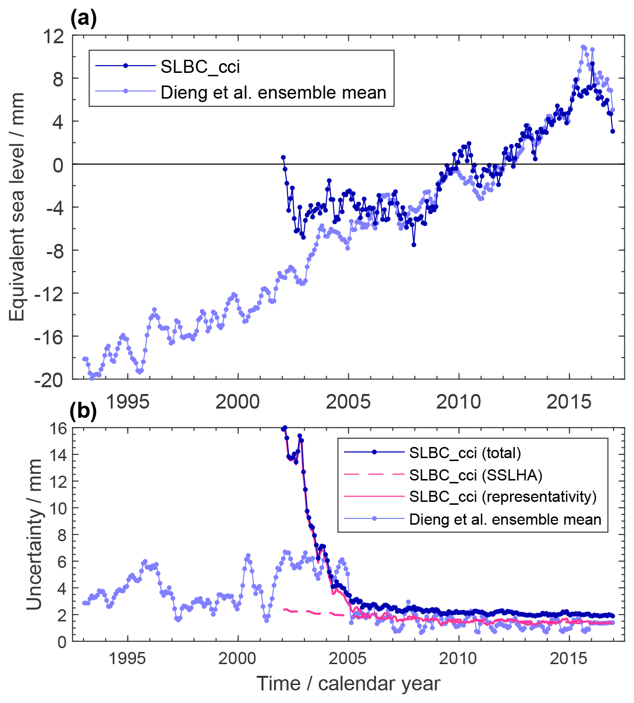
Figure 2(a) Global (65∘ N to 65∘ S) mean steric-sea-level height anomaly time series at monthly resolution. Dark blue: dataset generated within SLBC_cci based on Argo data and the CCI SST product. Light blue: update of the ensemble mean product by Dieng et al. (2017). Changes are expressed with respect to the mean of the reference interval of 2006–2015. (b) Uncertainties assessed for the estimates in (a). Pink curves (dashed and full lines) show the uncertainty contribution from the SSLHA (steric-sea-level height anomaly) uncertainty and from the global representativity uncertainty, respectively.
3.2.2 SLBC_cci steric product
Within SLBC_cci, the calculation scheme for the steric-sea-level change based on Argo data was updated from that described by von Schuckmann and Le Traon (2011). Formal propagation of uncertainty was included following JCGM (2008, their Eq. 13) in which an overall uncertainty estimate is obtained by propagating and combining the evaluations of uncertainty associated with each source.
Methods and product
The steric-thickness anomaly for a layer l of water with density ρl is , where hl,c is the steric thickness of a layer with climatological temperature and salinity and is the “steric thickness” of the layer relative to a layer of reference density ρ0 and reference height Δz0. The thickness can therefore be written in terms of layer density ρl and climatological density for the layer ρl,c as
The monthly mean steric-thickness anomaly for layer l is found as the optimum combination of the steric-thickness anomaly calculations from all the valid profiles in the grid cell for the month. Let the individual anomaly calculations be collected in a vector xl. The optimum estimate is then given by the following collection of equations:
where i is a column vector of ones, wl is the vector of weights appropriate to a minimum error variance average, and is the error covariance matrix of the steric-thickness anomaly estimates.
The error covariance matrix is needed for the optimal calculation of the monthly average in Eq. (12), as well as for the evaluation of uncertainty discussed below. To estimate this matrix, we need to be clear about what “error” means here: it is the difference between the steric-thickness anomaly for the layer from a single profile (Argo or climatological) and the (unknown) true cell-month mean. This difference therefore has two components: the measurement error in the profile, characterised by an error covariance , and a representativeness error arising from variability within the cell month . The measurement error covariance is the smaller term and was modelled to be independent between profiles within the cell (neglecting the fact that on occasion a single Argo float will contribute more than one profile within a given cell in a month). The representativeness error covariance was modelled assuming that this error has an exponential correlation form with a length scale of 2.5∘ and timescale of 10 d.
It is relatively common to have layers with no observations, sometimes in the upper ocean and often at depth. Conditional climatological profiles were used as an additional “observation” to fill in information for missing-data layers. The climatology of profiles was conditioned by the observed SST from Merchant et al. (2019), which essentially has negligible sampling uncertainty at monthly cell-average scales. The SST information constrains the upper-ocean profile to a degree determined by the vertical correlation of variability, which is variable in time and place according to the mixed-layer depth. The uncertainty in the conditional climatological profile is the variability. Examples of an unconditional and conditional climatological profile are shown in Fig. 3. For this particular month (August), year (2003), and location (30.5∘ N, 9.5∘ E), the SST is about 2 ∘C below the climatological value. The conditioning is strong for the upper ∼ 50 m of the ocean, and within this modest depth range the conditioned profile is realistic given the SST (approximately isothermal over a mixed layer). The uncertainty is reduced at the surface, where the cell-month SST is well known from the satellite data. Below about 150 m, the effect of conditioning decays towards zero (conditioned and unconditioned profiles converge).

Figure 3Example of the effect of conditioning climatology using SST from SST_cci, for a single time and location (30.5∘ N, 9.5∘ E; August 2003). Unconditioned (blue) and conditioned (orange) temperature profiles with their uncertainty ranges (shaded blue).
Including SST information slightly reduces uncertainty and affects steric height in the mixed layer often enough to influence the global mean. Over the period 2005–2018 the trend in steric height is larger using SST-conditioned climatological profiles than when using a static climatology as the prior. The use of static climatology to fill gaps in Argo profiles has been shown to cause systematic underestimates of trends in the literature (e.g. Ishii and Kimoto, 2009). Inclusion of SST conditioning to the climatology mitigates the over-stabilising effect.
The steric-sea-level height anomaly (SSLHA) was calculated for every month from January 2002 to December 2017 in a global grid of 5∘ × 5∘ resolution. For a given cell month, the SSLHA is the sum of the layer-by-layer estimates of steric-thickness anomaly, i.e. . By concatenating vectors and xl for all the layers into a vector of weights w and a vector of thicknesses x, we can write the following equivalent equation:
This form makes it more clear how to estimate the uncertainty in the SSLHA, which is
To evaluate the uncertainty we need to formulate Sx. The diagonal blocks corresponding to each layer in Sx are the matrices that have already been calculated on a layer-by-layer basis. Assumptions about the error correlations between layers are then required in order to complete the off-block-diagonal elements of Sx. Conservative assumptions were made:
-
Measurement errors are perfectly correlated vertically in a given profile; this is equivalent to saying that the sensor calibration bias dominates all other sources of measurement uncertainty in each profile.
-
Representativity errors are perfectly correlated vertically.
Having obtained cell-month mean SSLHA estimates and associated uncertainty, the global mean steric-sea-level height anomaly ΔSLSteric is the area-weighted average of the available gridded SSLHA results. ΔSLSteric was calculated over the range 65∘ S to 65∘ N, consistent with other budget elements.
Figure 2a shows the ΔSLSteric time series from the SLBC_cci product. While from 2005 onwards, the trends of the SLBC_cci product and the ensemble mean product (cf. Table A1) as well as their interannual behaviour are similar, the SLBC_cci product shows little change prior to 2005. This difference and its reflection by the uncertainty characterisation are discussed further below.
Uncertainty assessment
The uncertainties of the available cell-month mean SSLHA estimates were propagated to ΔSLSteric. In any given month, there are missing SSLHA cells, through lack of sufficient Argo profiles. Using ΔSLSteric estimated from the available SSLHA cells as an estimate for the global steric-sea-level anomaly introduces a global representativity uncertainty. Moreover, the global sampling errors are correlated month to month because the sampling distribution evolves over the course of several years towards near-global representation. To evaluate the global representativity uncertainty and serial correlation, the sampling pattern of sparse years was imposed on near-complete fields: the standard deviation of the difference in global mean with the two sampling patterns is a measure of uncertainty. The correlation between the sample-driven difference in consecutive months was found to be 0.85. The time series of the global representativity uncertainty, the uncertainty propagated from the gridded SSLHA uncertainty (which has no serial correlation), and this correlation coefficient combine to define a full error covariance estimate to be obtained for the ΔSLSteric time series.
Figure 2b shows the two components of uncertainty (global representativity and propagated SSLHA uncertainty) together with the total uncertainty. The global representativity uncertainty dominates prior to 2005 and is very large in 2002 and 2003. This reflects how sparse and unrepresentative the sampling by the Argo network was at that early stage.
Given the large representativity uncertainty prior to 2005, the absence of an increase in the SLBC_cci steric record during that time is thus understood to arise from global sampling error and is consistent with the global sampling uncertainty. The SLBC_cci steric time series and the ensemble mean steric time series are consistent given the evaluated uncertainties throughout the record. In addition, the evaluated uncertainties for the two time series with their different ways of uncertainty assessment are remarkably similar for the period of the established Argo network starting in 2005, giving confidence in the validity of two very distinct approaches to uncertainty characterisation.
The use of a formal-uncertainty framework allows separation of distinct uncertainty issues, namely, our ability to parameterise and estimate the various uncertainty terms, our ability to estimate the error covariance, and the model for propagation of error at each successive step.
Two aspects of the uncertainty model are recognised to be potentially optimistic: the modelling of measurement errors as independent between profiles rather than platforms and the use of only 10 years for assessing interannual variability. Two assumptions are potentially conservative: measurement errors in salinity and temperature were combined in their worst-case combination, and representativity errors in profiles are assumed to be fully correlated vertically, whereas in reality they are likely to decorrelate over large vertical separations.
A significant output of the uncertainty modelling of the steric component is the error covariance matrix for the time series. It enables proper quantification of the change during the time series. We employed the time-variable uncertainties to determine the linear trend in a weighted regression according to Eq. (10). Without weighting, the global sampling error prior to around 2005, noted above, would bias any fitted trend result. Use of the error covariance matrix enables proper quantification of the uncertainty in the trend calculation by propagating the error covariance matrix through the trend function. Without this, the serial correlation in the global sampling error would be neglected, and the calculated trend uncertainty would be an underestimate.
3.2.3 Deep-ocean steric contribution
For the deep ocean below 2000 m depth, the steric contribution was assessed as a linear trend of 0.1 ± 0.1 mm yr−1 following the estimate by Purkey and Johnson (2010) corroborated by Desbruyères et al. (2016). Note that this estimate is based on sparse in situ sampling. Corresponding evolutions of the ocean observing system are under way (Roemmich et al., 2019). This deep-ocean contribution is included in the ensemble mean steric product described in Sect. 3.2.2. This deep-ocean component is added to the Argo-based SLBC_cci steric product described in Sect. 3.2.1 (which is for depths < 2000 m) in order to address the full-ocean steric contribution.
3.3 Ocean-mass change
3.3.1 Methods and product
Time series of ocean-mass change (OMC), in terms of anomalies with respect to the 2006–2015 reference period, were generated from monthly gravity field solutions of the GRACE mission (Tapley et al., 2019). Similar to previous analyses (Johnson and Chambers, 2013; Uebbing et al., 2019) we used spherical harmonic (SH) GRACE solutions in order to have full control over the methodology and uncertainty assessment. Greater detail is provided by Horwath et al. (2019).
The following GRACE monthly gravity field solutions series were considered:
-
ITSG-Grace2018 (Kvas et al., 2019; Mayer-Gürr et al., 2018) from Institut für Geodäsie, Technische Universität Graz, Austria, with maximum SH degree 60 (data source: http://ftp.tugraz.at/outgoing/ITSG/GRACE/ITSG-Grace2018/monthly/monthly_n60, last access: 13 January 2022)
-
CSR RL06 from the Center for Space Research at the University of Texas, Austin, Texas, USA; GFZ RL06 from the Helmholtz Centre Potsdam GFZ (GeoForschungsZentrum) German Research Centre for Geosciences, Germany; and JPL RL06 from the Jet Propulsion Laboratory, Pasadena, California, USA, all with maximum SH degree 60 (data source: https://podaac.jpl.nasa.gov/GRACE, last access: 13 January 2022).
We chose ITSG-Grace2018 as the preferred input SH solution because it showed the lowest noise level among all releases considered, with no indication for differences in the contained signal (Groh et al., 2019b).
Gravity field changes were converted to equivalent water height (EWH) surface mass changes according to Wahr et al. (1998). The total mass anomaly over an area like the global ocean was derived by spatial integration of the EWH changes. We used the unfiltered GRACE solutions in order to avoid damping effects from filtering. A 300 km wide buffer zone along the ocean margins was excluded from the spatial integration. Around islands, the buffer was applied if their surface area exceeds a threshold, which was set to 20 000 km2 in general and 2000 km2 for near-polar latitudes beyond 50∘ N or 50∘ S. The integral was subsequently scaled by the ratio between the total area of the ocean domain and the buffered integration area. This scaling is based on the assumption that the mean EWH change in the buffer equals the mean EWH change in the buffered ocean area. Effects of violations to this assumption are included in the uncertainty assessment (see further below).
Modelled short-term atmospheric and oceanic mass variations are accounted for within the gravity field estimation procedure (Flechtner et al., 2014; Dobslaw et al., 2013) and are not included in the monthly solutions. To retain the full mass variation effect, the monthly averages of the modelled atmospheric and oceanic dealiasing fields were added back to the monthly solutions by using the so-called GAD products (Flechtner et al., 2014). We subsequently removed the spatial mean of atmospheric surface pressure over the full-ocean domain. Our investigations confirmed findings by Uebbing et al. (2019) on the methodological sensitivity of this procedure. If the GAD averages were calculated over only the buffered area, OMC trends would be about 0.3 mm yr−1 higher than for our preferred approach.
Table 1OMC linear trends (millimetre equivalent of global mean sea level per year) over January 2003–August 2016 from different GRACE solutions. Each column uses a different GIA correction as indicated in the header line. The first four lines of data show results from different SH solution series generated within SLBC_cci. Numbers in brackets are for the ocean domain between 65∘ N and 65∘ S. The last two lines show external products, namely the ensemble mean of the updated time series by Johnson and Chambers (2013) and the GSFC RL06v01 mascon solution. The last column shows the assessed total uncertainty of the trend. The preferred solution is printed in bold font. n/a: not applicable.
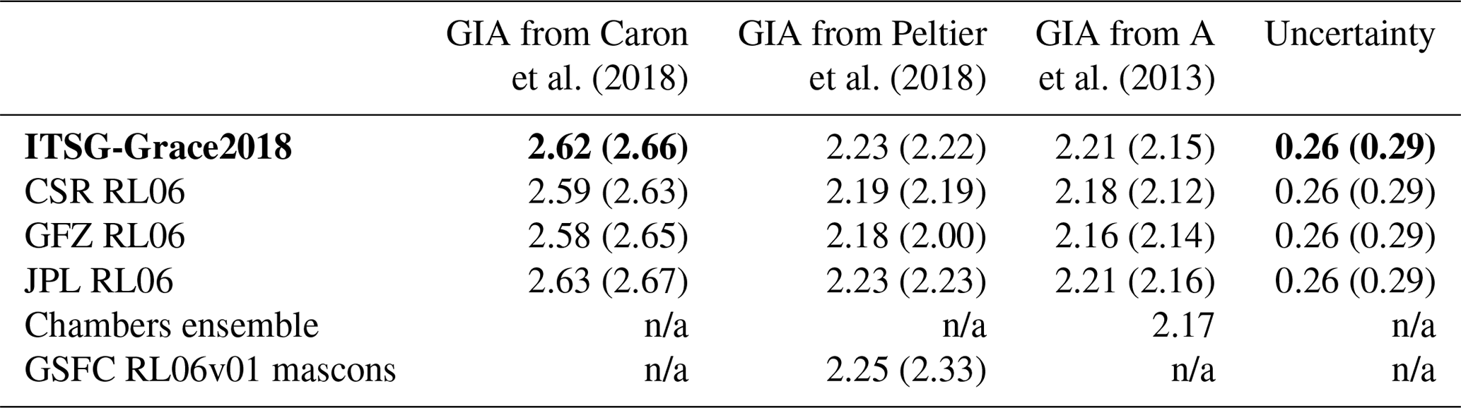
GIA implies redistributions of solid-Earth masses and (to a small extent) of ocean masses. We corrected the gravity field effect of GIA-related mass redistributions by using three different GIA modelling results: the model by A et al. (2013), based on ICE-5Gv2 glaciation history from Peltier (2004); the model ICE-6G_D (VM5A) by Peltier et al. (2015, 2018); and the mean solution by Caron et al. (2018). The correction was applied on the level of the SH representation. Our preferred GIA correction is the one by Caron et al. (2018). It is based on the ICE-6G deglaciation history (Peltier et al., 2015), while the model by A et al. (2013) is based on its predecessor model, ICE-5G. Furthermore, while the models by A et al. (2013) and Peltier et al. (2015) are single GIA models, the solution by Caron et al. (2018) arises as a weighted mean from a large ensemble of models, where the glaciation history and the solid-Earth rheology have been varied and tested against independent geodetic data to provide probabilistic information. Table 1 demonstrates the sensitivity of GRACE OMC solutions to the GIA correction.
In order to include the degree-one components of global mass redistribution (not determined by GRACE), we implemented the approach by Sun et al. (2016), which combines the GRACE solutions for degree n ≥ 2 with assumptions on the ocean-mass redistribution. The results depend on the input GRACE solution series and, more importantly, on the adopted GIA model. While GRACE Technical Note TN13 provides degree-one time based on the Sun et al. (2016) method, their input is fixed to the CSR, GFZ, or JPL solutions and the ICE-6G_D GIA model. By our own implementation we generate degree-one series that are consistent with our choice of GRACE solution series (such as ITSG-Grace2018) and GIA models (such as by Caron et al., 2018). We also replaced GRACE-based C20 (the Earth flattening component of SH degree 2 and order 2) components with results from satellite laser ranging (SLR) (Loomis et al., 2019a, https://podaac-tools.jpl.nasa.gov/drive/files/allData/grace/docs/TN-14_C30_C20_GSFC_SLR.txt, last access: 13 January 2022).
Figure 4a shows our preferred time series of the mass contribution to sea level (see Fig. 10 for a time series where the seasonal signal is subtracted). The overall trend at 2.62 ± 0.26 mm yr−1 over P2 is superimposed by a seasonal signal with 10.3 mm amplitude of annual sinusoid and by interannual variations like a drop by about 6 mm sea-level equivalent between 2010 and 2011.
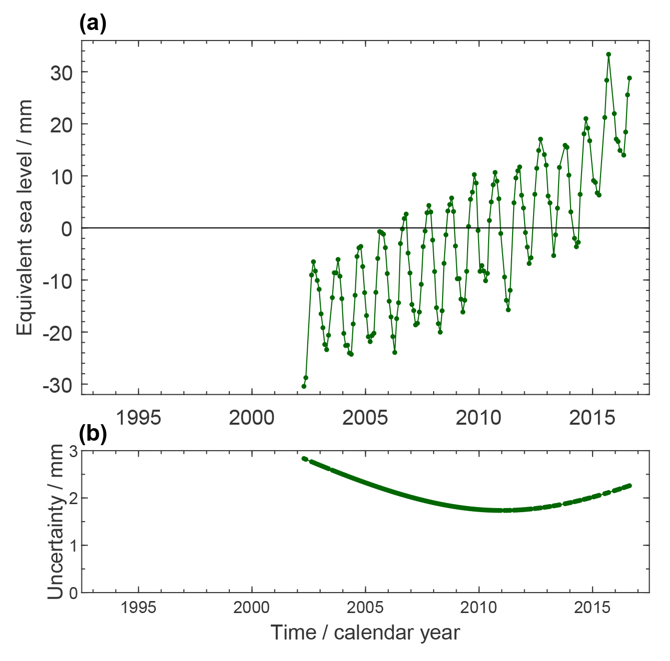
Figure 4(a) Ocean-mass component of GMSL change, derived from the ITSG-Grace2018 spherical harmonic GRACE monthly solutions with a GIA correction according to Caron et al. (2018). Mass change of the global ocean is expressed in terms of equivalent GMSL change with respect to the mean of the reference interval of 2006–2015. Time series are shown in their original temporal sampling where some months are missing. (b) Uncertainties assessed for the estimates in (a).
Overall, integrated OMC time series were generated from four series of SH GRACE solutions, using three GIA corrections (and the option of no GIA correction), for the global ocean and the ocean domain between 65∘ N and 65∘ S. For comparison, we also considered OMC time series from two external sources: global OMC time series from CSR, GFZ, and JPL SH solutions by Johnson and Chambers (2013), updated by Don Chambers on 6 November 2017 and made available by the author on 26 January 2018, and Goddard Space Flight Center (GSFC) mascon solutions RL06v01 (release 6, version 1) (Loomis et al., 2019b), dedicated for ocean-mass research (data source: https://earth.gsfc.nasa.gov/geo/data/grace-mascons, last access: 13 January 2022). Time series of total OMC from GSFC mascons were derived by the weighted integral over all oceanic points, using the ocean–land point-set mask contained in the solutions (but excluding the Caspian Sea). Integrated OMC was then divided by the total area over the corresponding oceanic mascons.
3.3.2 Uncertainty assessment
The following sources of uncertainty are relevant (cf. Groh and Horwath, 2021):
-
GRACE errors: errors in the GRACE observations as well as in the modelling assumptions applied during GRACE processing propagate into the GRACE products.
-
Errors in C20 and degree-one terms: errors in these components, due to their very large-scale nature and possible systematic effects are particularly important for global OMC applications (cf. Quinn and Ponte, 2010; Blazquez et al., 2018; Loomis et al., 2019a).
-
The impact of GIA on GRACE gravity field solutions is a significant source of signal and error for mass change estimates. Current models show strong discrepancies (Quinn and Ponte, 2010; Chambers et al., 2010; Tamisiea and Mitrovica, 2011; Rietbroek et al., 2016; Blazquez et al., 2018).
-
Leakage errors arise from the vanishing sensitivity of GRACE to small spatial scales (high SH degrees). In SLBC_cci, GRACE data were used up to a degree 60 (∼ 333 km half wavelength). As a result, signal from the continents (e.g. ice-mass loss) leaks into the ocean domain. Differences in methods to avoid (or repair) leakage effects can amount to several tenths of a kg m−2 yr−1 in regional OMC estimates (e.g. Kusche et al., 2016). Our buffering approach does not fully avoid leakage. Moreover, the upscaling of the integrated mass changes to the full-ocean area is based on the assumption that the mean EWH change in the buffer is equal to the mean EWH change in the buffered ocean integration kernel.
We adapted the uncertainty assessment approach used for GRACE-based products of the Antarctic Ice Sheet CCI project (Groh and Horwath, 2021). We modelled errors as the combination of two components distinguished by their temporal characteristics: temporally uncorrelated noise, with variance assumed equal for each month, and systematic errors of the linear trend, with an associated uncertainty σtrend. This model is a simplification, as it does not consider autocorrelated errors other than errors that evolve linearly with time. The uncertainty σtotal(t) per epoch t in a time series of mass anomalies z(t) is approximated as
where t0 is the centre of the reference interval to which z(t) refers.
The noise was assessed from the GRACE OMC time series themselves as detailed by Groh et al. (2019a). The detrended and deseasonalised time series were high-pass-filtered in the temporal domain. The variance of the filtered time series was assumed to be dominated by noise. This variance was scaled by a factor that accounts for the dampening of uncorrelated noise variance imposed by the high-pass-filtering process. The assessed noise component comprises uncorrelated errors from all uncertainty sources except for GIA, which is considered purely linear in time.
The systematic errors of the linear trends are assumed to originate from errors in degree-one components, C20, the GIA correction, and leakage. The related uncertainties were assessed for each source individually and summed in quadrature.
Trend uncertainties associated with GIA, degree-one, and C20 were assessed individually based on the spread of a small ensemble of different options to incorporate these effects. The ensemble standard deviation was taken as the associated standard uncertainty. The GIA uncertainty assessment used the ensemble of the three GIA correction options mentioned above and in Table 1. For the degree-one uncertainty assessment we made a choice of 10 different series in the attempt to represent a balanced sample of different methods and input datasets. This choice includes three series from our implementation of the method by Sun et al. (2016) using the ITSG-Grace2018 GRACE solutions and the GIA model by A et al. (2013), Peltier et al. (2018), and Caron et al. (2018), respectively; the three TN13 series using CSR, GFZ, and JPL GRACE solutions, respectively; the series originally provided by Sun et al. (2016); the series derived from SLR by Cheng et al. (2013); the series from the global combination approach by Rietbroek et al. (2016); and the series derived earlier for CSR RL05 solutions according to the method by Swenson et al. (2008). Likewise, for the C20 uncertainty assessment we made a choice of the following seven series: five series based on SLR by, respectively, Loomis et al. (2019a), Cheng and Ries (2017), Bloßfeld et al. (2015), König et al. (2019), and Cheng et al. (2013); one series from a combined analysis of SLR and GRACE by Bruinsma et al. (2010); and one series based on the GRACE model combination by Sun et al. (2016).
To estimate the uncertainty that arises from leakage, in conjunction with buffering and rescaling, we performed a simulation study based on synthetic mass change data from the ESA Earth System Model (ESM; Dobslaw et al., 2015). The ESM data were processed according to the settings of the SLBC_cci OMC analysis, and the results (simulated observations) were compared with the OMC that arises from the full-resolution ESM data (simulated truth). In order to derive statistics for multi-year trends, we calculated linear trends of the simulated observations and of the simulated truth and of their misfit for every interval of a length between 9 and 12 years contained in the ESA ESM period. The weighted RMS (root mean square) of misfits over all intervals was taken as the estimate of the leakage error uncertainty.
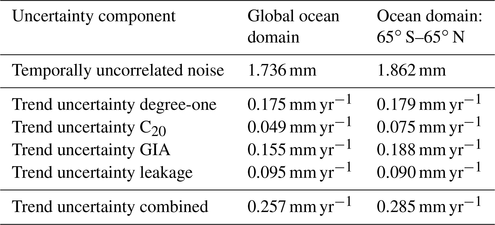
Results of the uncertainty assessment for the ITSG-Grace2018-based OMC solutions are summarised in Table 2. Figure 4b shows the time-dependent uncertainties associated with the ocean-mass contribution time series. They reflect their construction by Eq. (16), where away from 2011.0, the uncertainty of the linear trend contributes an increasing share.
Table 2Assessed uncertainty components for the OMC solutions based on the ITSG-Grace2018 SH GRACE solutions.
The GRACE-based OMC products described and used here adopt recent standards concerning the degree-one and C20 series used as well as the inclusion of ICE-6G_D (instead of ICE-6G_C) in our comparison of GIA corrections. The products are an update to previous estimates by Horwath et al. (2019). Our estimated global OMC trends (for identical periods) are larger than the previous estimates. The difference (updated trend minus previous trend) is mainly due to the updated degree-one treatment and depends on the GIA model involved in the degree-one estimation. Incidentally, this difference is largest for our preferred choice of the GIA model by Caron et al. (2018), where the difference amounts to 0.43 mm yr−1. This difference is outside the assessed 1σ uncertainty but inside the 1.65σ range that would correspond to a 90 % confidence range. The sensitivity of GRACE-based OMC trends observed here and in previous studies (Blazquez et al., 2018; Uebbing et al., 2019; Dobslaw et al., 2020) corroborates the uncertainty on the order of a few tenths of a millimetre per year that remains associated with GRACE-based OMC trends.
3.4 Glacier contribution
3.4.1 Methods and product
The glacier mass change estimate was derived by updating the global glacier model (GGM) of Marzeion et al. (2012). Annually reported direct mass balance observations (using the glaciological method) are available for only a few hundred of the roughly 215 000 existing glaciers (Zemp et al., 2019). Global-scale geodetic, altimetric, and gravimetric observations are limited to the most recent decades (e.g. Bamber et al., 2018). Estimates of geodetic glacier mass balance back into the 1960s are available only at regional scale and are more disperse (e.g. Maurer et al., 2019; Zhou et al., 2018). The overall objective of the model approach is to use observations of glacier mass change for calibration and validation of the glacier model, which then translates information about atmospheric conditions into glacier mass change, taking into account various feedbacks between glacier mass balance and glacier geometry. This enables a reconstruction of glacier change that is complete in time and space and that has higher temporal resolution than the observations (here, we use monthly output). In our analysis, we included all glaciers outside of Greenland and Antarctica and separately reconstructed the glacier change for Greenland peripheral glaciers.
As initial conditions, we used glacier outlines obtained from the Randolph Glacier Inventory (RGI) version 6.0 (updated from Pfeffer et al., 2014). The timestamp of these outlines differs between glaciers but typically is around the year 2000. To obtain results before this time, the model uses an iterative process to find that glacier geometry in the year of initialisation (e.g. 1901) that results in the observed glacier geometry in the year of the outline's timestamp (e.g. 2000) after the model was run forward.
The model relies on monthly temperature and precipitation anomalies to calculate the specific mass balance of each glacier. It uses the gridded climatology of New et al. (2002) as a baseline. Here, we used seven different sources of atmospheric conditions (as well as their mean) as boundary conditions (Harris et al., 2014; Saha et al., 2010; Compo et al., 2011; Dee et al., 2011; Kobayashi et al., 2015; Poli et al., 2016; Gelaro et al., 2017). Temperature is used to estimate the ablation of glaciers following a temperature-index melt model and to estimate the solid fraction of total precipitation, which is used to estimate accumulation. Glacier area and length change are estimated following mass change based on volume–area–time scaling, allowing for a delayed response of glacier geometry to glacier mass change. A detailed description of the model is provided by Marzeion et al. (2012).
There are four global model parameters that need to be optimised: (i) the air temperature above which melt of the ice surface is assumed to occur; (ii) the temperature threshold below which precipitation is assumed to be solid; (iii) a vertical precipitation gradient used to capture local precipitation patterns not resolved in the forcing datasets; and (iv) a precipitation multiplication factor to account for effects from (among other processes) wind-blown snow and avalanching, which are not resolved in the forcing dataset. For each of the eight forcing datasets cited above, we performed a multi-objective optimisation for these four parameters, using a leave-one-glacier-out cross validation to measure the model's performance on glaciers for which no mass balance observations exist. We used annual in situ observations from about 300 glaciers, covering a total of almost 6000 mass balance years (WGMS, 2018). In the optimisation, the temporal correlation of observed and modelled mass balances is maximised; the temporal variance of modelled mass balances is brought close to that of observed mass balances (aiming for a realistic sensitivity of the model to climate variability and change); and the model bias is minimised (to avoid an artificial trend in modelled glacier mass). Using the mean of the seven atmospheric datasets described above results in the overall best model performance. Compared to the results in Marzeion et al. (2012), the correlation of annual glacier mass change was increased from 0.60 to 0.64; the bias was changed from 5 to −4 kg m−2 (both statistically indistinguishable from zero); and the ratio of the temporal variance of modelled and observed mass balances was improved from 0.83 to 1.00.
The model output for each glacier is aggregated on a regular 0.5∘ × 0.5∘ grid, where the mass change of each glacier is assigned to the grid cell that contains the glacier's centre point, even if the glacier might cover several grid cells (the GGM does not calculate the spatial distribution of mass changes of a glacier so that a more accurate spatial assignment to the grid is not possible). Regional or global values of glacier mass change were obtained by summing over the region of interest.
Figure 5a shows the global glacier contribution to GMSL anomalies (see Figs. 10 and 12 for time series after subtraction of the seasonal signal). The glacier contribution has a linear trend of 0.64 ± 0.03 mm yr−1 over P1, where the positive rate increases from the first half to the second half of the period. Interannual variations are less pronounced than for other budget elements.
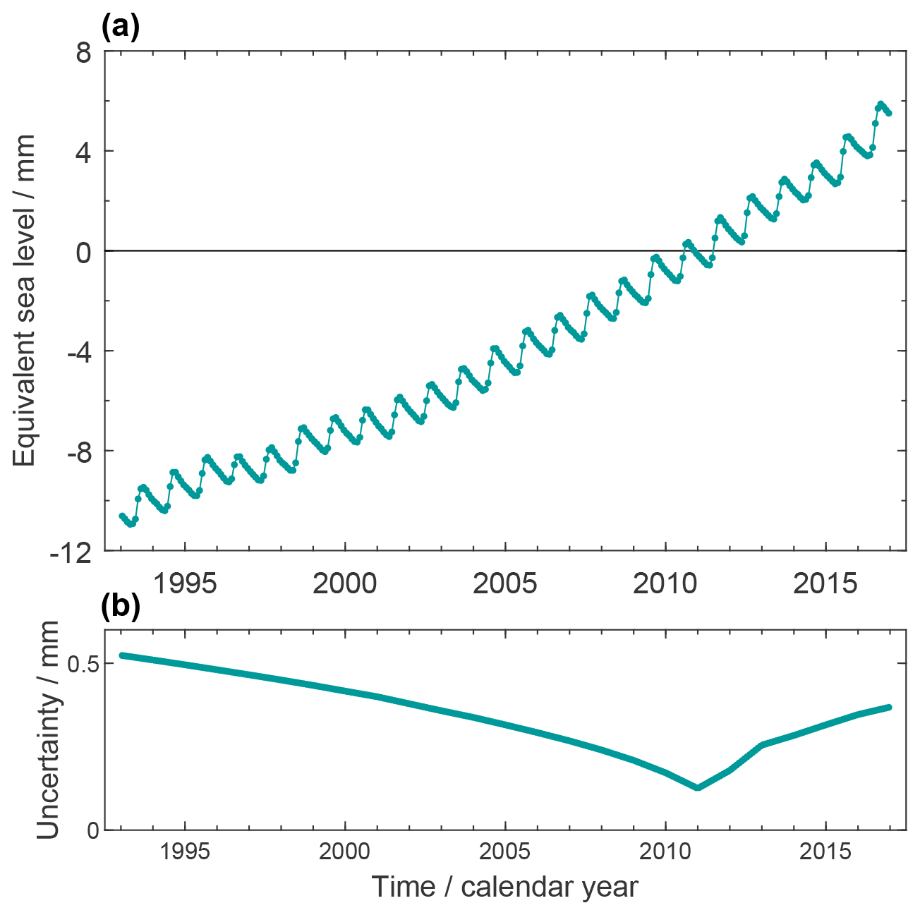
Figure 5(a) Global glacier mass contribution to GMSL assessed by the GGM at a monthly resolution. Peripheral glaciers in Greenland and Antarctica are not included. Glacier mass change is expressed in terms of equivalent GMSL change with respect to the mean of the reference interval of 2006–2015. (b) Uncertainties assessed for the estimates in (a).
3.4.2 Uncertainty assessment
The root mean square error obtained during the cross validation was propagated through the model. Since the evaluation of the model results does not indicate any temporal or spatial correlation of the model errors, the uncertainty of temporal and spatial mass change aggregations was calculated assuming independence of the model errors, i.e. by taking the root of the summed squares of each glacier's (and year's) uncertainty.
Uncertainties of mass anomalies with respect to the mean over the 2006–2015 interval were approximated by uncertainties of anomalies with respect to the centre of the interval, 2011.0. Uncertainties of yearly mass change rates were aggregated (as the root sum square) forward or backward from 2011.0 to the specific epochs. Figure 5b shows the uncertainties per epoch, reflecting this aggregation from 2011.0. Uncertainties of multi-year linear trends were calculated as follows: the uncertainties of yearly rates of mass change were aggregated in time over the interval of interest, leading to an uncertainty of cumulated mass change over the interval of interest, which was subsequently divided by the length of the interval. That is, the trend uncertainty was calculated as the root sum square of yearly rate uncertainties, divided by the interval length.
3.5 Greenland contribution
Changes of land ice masses in Greenland comprising the GrIS and peripheral glaciers are assessed in two ways: by GRACE (Sect. 3.5.1) and by a combination of satellite altimetry for the GrIS and glacier modelling for the peripheral glaciers (Sect. 3.5.2 and 3.5.3). Results from those complementary assessments shown in Fig. 6 are collectively discussed at the end of this section.

Figure 6(a) Greenland ice-mass contribution to GMSL assessed from GRACE (dark green) and from the combination of altimetry and GGM (light green). The altimetry-based assessment for the ice sheet (blue) and the GGM-based assessment for the peripheral glaciers (brown) are also shown. Ice-mass change is expressed in terms of equivalent GMSL change with respect to the mean of the reference interval of 2006–2015. GRACE-based time series are shown in their original temporal sampling where some months are missing. (b) Uncertainties assessed for the estimates in (a).
3.5.1 GRACE-based estimates
The GRACE-based product developed at DTU Space (Technical University of Denmark) within the Greenland Ice Sheet CCI project is used to provide mass change estimates for the GrIS from GRACE monthly gravity field solutions. The quasi-monthly GRACE-based mass anomaly estimates (grids and basin time series) are available at https://climate.esa.int/en/projects/ice-sheets-greenland/ (last access: 13 January 2022). Comprehensive descriptions and references are given by Barletta et al. (2013), Horwath et al. (2019), and Mottram et al. (2019).
Methods and product
An inversion technique was used to obtain monthly mass anomalies for all of Greenland from each of the available GRACE monthly solutions, with the approach described in Barletta et al. (2013). An icosahedral grid of point masses, each representing an area of ∼ 20 km radius, was inverted in order to fit the gravity observations at the satellite altitude. The limited ∼ 300 km resolution of the GRACE monthly solution requires inversion for ice-mass changes over the whole GrIS including peripheral glaciers, whose contribution cannot be isolated independently. For this work the CSR RL06 monthly solutions were used, with a maximum degree and order of 96, and prior to the inversion the prescribed C20 and degree-one corrections were applied, together with an anisotropic filtering (DDK3 from Kusche et al., 2009). Mass changes of glaciers outside Greenland were co-estimated to minimise their leakage into the Greenland ice-mass change estimates.
Our inversion did not include a GIA correction. We separately calculated the effect of GIA on our inversion. Based on the Caron et al. (2018) GIA solution (chosen for consistency with the OMC estimate; cf. Sect. 3.3) we obtained a GIA effect of 7.5 Gt yr−1. This linear trend was subtracted from the time series.
Uncertainty assessment
GRACE-based products are provided with error estimates based on the approach developed by Barletta et al. (2013). The uncertainties were propagated from the errors in GRACE monthly solutions, leakage errors due to GRACE-limited spatial resolutions, and errors in the models used to account for degree-one contributions and the GIA correction. In detail, the uncertainty related to GRACE solutions was obtained in a Monte Carlo-like approach, with 200 simulations for Stokes coefficients selected from a zero-mean normal distribution and the standard deviation from the GRACE CSR RL06 Level 2 solution.
3.5.2 Altimetry-based estimates
Methods and product
The surface elevation changes estimates are based on satellite radar altimeter observations for the period 1992–2017 and include data from the missions ERS-1, ERS-2, Envisat, and CryoSat-2. The temporal evolution of surface elevation is estimated by a combination of crossover, repeat-track, and least-squares methods covering the entire GrIS and for the entire time span covered by the different missions, on a 5 km common uniform grid (Sørensen et al., 2018). The different characteristics of the missions (the conventional radar altimetry of the ERS-1, ERS-2, and Envisat missions and the novel interferometric SAR – synthetic-aperture radar – altimetry of CryoSat-2) and the different orbital characteristics call for special care in the combinations of the different datasets and in the determination of the uncertainties.
Before an ice-sheet-wide estimate of volume change can be converted into ice sheet mass balance, contributions which are not related to ice-mass change must be corrected for. These contributions include factors such as changes in firn compaction rates, GIA, and elastic uplift. Such a correction method was first applied for satellite ICESat (Ice, Cloud and land Elevation Satellite) lidar observation (Sørensen et al., 2011). As Ku-band radar altimetry is subject to weather-induced changes in subsurface penetration depth of snow-covered areas (Nilsson et al., 2015), we here chose to apply a different calibration procedure instead of the direct correction fields. This approach follows that of Simonsen et al. (2021). The calibration period is the era of ICESat (2003–2009), where the ICESat laser altimeter provides precise estimates of surface elevation change without surface penetration and ENVISAT provides similar estimates subject to surface penetration. The spatial differences between the ICESat and ENVISAT mass estimates provides the input for a calibration field (initial radar-volume mass balance) which can be applied to the full time series of elevation changes based on satellite radar altimeter observations for the period 1992–2017.
Following the calibration procedure described above, we computed monthly grids of mass change rates at 100 × 100 km2 resolution for the entire main GrIS. The peripheral glaciers (connectivity level 0 and 1 according to Rastner et al., 2012) were excluded from the grid. For each epoch, the mass rates of the grid cells were added to derive monthly mass change rates of the entire ice sheet. Time series of ice sheet mass anomalies with respect to the reference interval of 2006–2015 were then generated by cumulating the mass change rates in time and subtracting the mean over 2006–2015 from the cumulated time series.
The monthly grids were derived by applying a temporal window to aggregate the radar observations. For the ERS-1, ERS-2, and ENVISAT mission, this window is 5 years long. For CryoSat-2 the window is 3 years long. The monthly grids referred to the centre of the time window. This result in a smoothing of the time series to resolve climatic changes and not seasonal weather.
Uncertainty assessment
The error of the traditional altimetry-based mass-change estimates originates from different sources: uncertainty in the interpolation from point changes to ice-sheet-wide changes, uncertainty in the bedrock movement and in the firn compaction model, uncertainties due to the neglect of basal melt contributions, and of the possible ice accumulation above the equilibrium line altitude due to ice dynamics. For observations from radar altimetry, an additional source of uncertainty is the changing radar penetration in the firn column. The latter was reduced by the calibration approach applied here.
The overall uncertainty in the altimetry-derived mass change time series is provided as a conservative estimate based on converting the radar altimetry volume error into mass by ascribing ice densities to all grid cells. This estimate is assumed to be slightly overestimating the combined error of the five error sources.
Uncertainties of cumulated mass changes (in space as well as in time) were derived as follows: for the cumulation in space, standard uncertainties from all grid cells were added linearly. For the cumulation in time, uncertainties of mass change rates were aggregated (as the root sum square) forward or backward from 2011.0 to the specific epochs. Uncertainties of multi-year trends were calculated as the aggregated uncertainties of mass change rates over the interval of interest, divided by the interval length.
3.5.3 Altimetry–GGM combination
Unlike the GRACE-based assessment for Greenland, the altimetry-based assessment does not include Greenland peripheral glaciers. We therefore take the sum of the altimetry-based estimates for the ice sheet and GGM-based estimates for the peripheral glaciers to represent the total ice-mass changes in Greenland. The GGM methods and products and the related uncertainty assessments described in Sect. 3.4 were applied. The uncertainties of the sum of the two products were calculated as the root sum square of the uncertainties of the two summands.
The synthesis of assessed Greenland GMSL contributions in Fig. 6a shows that both the proper ice sheet and peripheral glaciers contribute significantly (0.43 ± 0.04 and 0.17 ± 0.02 mm yr−1, respectively, over P1). The rates of change vary interannually, peaking in 2011 and 2012. This is consistently reflected in the GRACE-based estimate and in the altimetry–GGM combination. The altimetry–GGM combination shows a somewhat larger trend over P2 than the GRACE-based estimate (0.89 ± 0.07 mm yr−1 versus 0.78 ± 0.02 mm yr−1) and does not resolve the annual cycle in the same way as GRACE, as the annual cycle is not resolved in the altimetry-based time series. The time-variable uncertainties of the altimetry-based and GGM-based time series (Fig. 6b) reflect the cumulation of uncertainties of rates of change backward and forward from the reference interval centre. The uncertainties of the GRACE-based time series reflect the superposition of a linear-trend uncertainty and an individual uncertainty for each monthly GRACE solution.
3.6 Antarctic contribution
Mass changes of the AIS are assessed in two ways: by GRACE (Sect. 3.6.1) and by satellite radar altimetry (Sect. 3.6.2). The results from the complementary assessments shown in Fig. 7 are collectively discussed in Sect. 3.6.2. The contribution from Antarctic peripheral glaciers is discussed in Sect. 3.8.
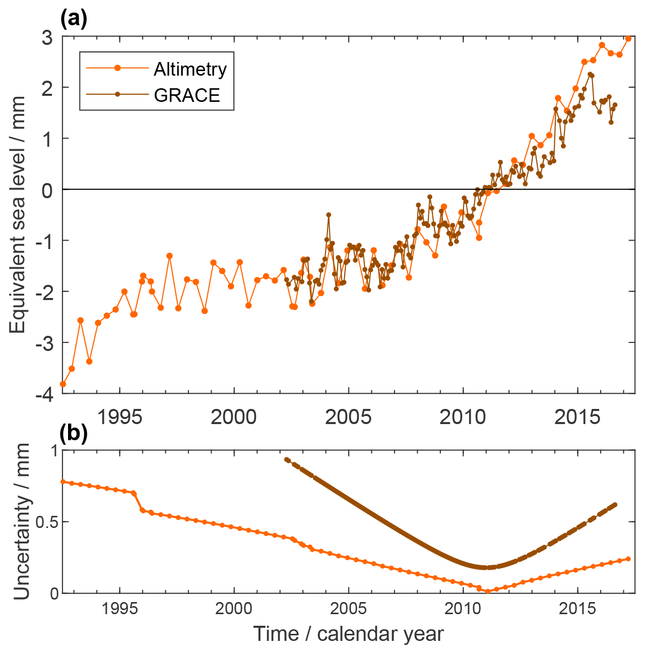
Figure 7(a) Antarctic Ice Sheet mass change contributions to GMSL from GRACE (dark orange) and altimetry (orange). Ice-mass change is expressed in terms of equivalent GMSL change with respect to the mean of the reference interval of 2006–2015. The temporal sampling is quasi-monthly (with a few months missing) for the gravimetric time series and 140-daily (with a few shorter time increments) for the altimetric time series. (b) Uncertainties assessed for the estimates in (a).
3.6.1 GRACE-based estimates
The GRACE-based product developed at Technische Universität Dresden within the Antarctic Ice Sheet CCI project is used to provide mass change estimates for the AIS from GRACE monthly gravity field solutions (Groh and Horwath, 2021). Quasi-monthly GRACE-based mass anomaly estimates (grids and basin time series) are available at https://climate.esa.int/en/projects/ice-sheets-antarctic/ (last access: 13 January 2022) or https://data1.geo.tu-dresden.de/ais_gmb (last access: 13 January 2022).
Methods and product
The AIS GRACE-based products were derived from the SH monthly solution series by ITSG-Grace2016 by Technische Universität Graz (Klinger et al., 2016; Mayer-Gürr et al., 2016) following a regional integration approach with tailored integration kernels that account for both the GRACE error structure and the information on different signal variance levels on the ice sheet and on the ocean (Groh and Horwath, 2021). The GIA correction adopted by these products was based on the regional model by Ivins et al. (2013). In Sect. 7.2 we address the trade-off between using global or regional GIA models for Antarctica.
Uncertainty assessment
The uncertainty assessment (Groh and Horwath, 2021) is analogous to that described for the GRACE OMC assessment in Sect. 3.3. For the AIS, the dominant source of uncertainty is the GIA correction. Uncertainties in the degree-one components and the C20 component of the gravity field are also important.
3.6.2 Altimetry-based estimates
Methods and data product
We computed Antarctic mass change from 1992 to 2017 using observations from four different satellite radar altimetry missions – ERS-1, ERS-2, ENVISAT, and CryoSat-2 – following the methodology described by Shepherd et al. (2019). For each mission, we computed elevation change from repeated elevation measurements during fixed epochs of 140 d on a polar stereographic grid using a plane fit method (McMillan et al., 2016). We applied a backscatter correction to remove the short-term fluctuations in elevation change correlated with changes in backscatter, and we combined the time series from different missions together by applying a cross-calibration technique. To convert our elevation change time series into a mass change time series, we first identified areas of ice dynamical imbalance in order to discriminate between changes occurring at the density of snow and ice. We defined these regions as areas with persistent elevation change that is significantly different from firn thickness change estimates derived from a semi-empirical firn densification model (Ligtenberg et al., 2011). Areas with an accelerated rate of ice thickness change were allowed to evolve through time. Based on this empirical classification, we converted our elevation change time series to a mass change time series by using a density of 917 kg m−3 in areas classified as ice and using spatially varying snow densities from the firn densification model in areas classified as snow. The mass anomalies for the West Antarctic Ice Sheet (WAIS), the East Antarctic Ice Sheet (EAIS), and the Antarctic Peninsula (APIS) at a 140 d resolution from 1992 to 2016 are available at http://www.cpom.ucl.ac.uk/csopr/ (last access: 13 January 2022).
Figure 7a shows the AIS GMSL contributions from the altimetry-based assessment as well as from the GRACE-based assessment. Over P1 (assessed from altimetry), the AIS contribution to GMSL is 0.19 ± 0.04 mm yr−1. Rates of change are much smaller from 1995 to 2006 and larger from 2006 onwards. Mass losses are dominated by mass losses in West Antarctica due to changing ice flow dynamics (cf. Shepherd et al., 2018). Over P2, the evolution of the AIS GMSL contribution from altimetry and GRACE is similar, with linear trends at 0.34 ± 0.04 and 0.27 ± 0.11 mm yr−1, respectively, overlaid by noise as well as a common interannual signal.
Uncertainty assessment
We assessed the uncertainties of our elevation change time series and convert them to a mass change uncertainty using the same time-evolving mask of areas of ice dynamical imbalance described in the previous section. At each epoch, we estimated the overall error of our elevation change as the sum in quadrature of systematic errors, time-varying errors, errors associated with the calibration between the different satellite missions, and errors associated with snowfall variability. The systematic errors refer to errors that affect the long-term elevation change trend. These may arise from short-term changes in the snowpack properties or from short-lived accumulation events that may not be accounted for in our plane fit model. We quantified the systematic errors as the standard error of the long-term rate of elevation change. The time-varying error refers to errors in the satellite measurements that might hinder our ability to measure elevation change at one particular epoch due to the measurement's precision or non-uniform sampling. We calculated these errors as the average standard error of elevation measurements. The inter-satellite bias uncertainties were computed as the standard deviations between modelled elevations during a 2-year period centred on each mission overlap. Finally, we quantified the snowfall variability uncertainty based on estimates from a regional climate model.
Cumulated mass changes and their uncertainties were originally generated with respect to the reference epoch of 1993.0, separately for the EAIS, the WAIS, and the APIS. To refer the product to the reference interval of 2006–2015, we subtracted the respective mean from the mass anomaly time series. We calculated uncumulated uncertainties by taking the differences between the uncertainties of consecutive epochs. We re-cumulated these uncertainties with respect to the centre of the reference interval, 2011.0, by linearly cumulating the uncumulated uncertainties, forward or backward, from 2011.0. Uncertainties of linear trends were calculated by linearly cumulating the uncumulated uncertainties over the interval of interest and division by the interval length. Uncertainties for the mass changes of the entire AIS were calculated as the root sum square of uncertainties for the EAIS, WAIS, and APIS.
Figure 7b shows the time-dependent uncertainties resulting from the cumulation with respect to the reference interval centre. The uncertainties of the GRACE-based estimates also shows reflect the model analogous to Eq. (16).
3.7 Land water storage
3.7.1 Methods and product
The LWS contribution is assessed with the global hydrological model (GHM) WaterGAP (Döll et al., 2003; Müller Schmied et al., 2014) in its latest version, WaterGAP2.2d (Müller Schmied et al., 2021). The model simulates daily water flows and water storage anomalies including the effects of human water use on a 0.5∘ × 0.5∘ grid (55 km × 55 km at the Equator and ∼ 3000 km2 grid cell) covering the whole land area except for Antarctica (we excluded model outputs over Greenland to avoid double-counting). Note that the Caspian Sea is not part of the model grid (based on the WATCH–CRU – Climatic Research Unit – land–sea mask) and thus not included in the assessment of the LWS component. Water flows are routed through a series of individual water storage compartments (Fig. 2 in Müller Schmied et al., 2021). Following the stream network defined by the global drainage direction map DDM30 (Döll and Lehner, 2002), streamflow is laterally routed until reaching the ocean or an inland sink. The model is calibrated against observed mean annual streamflow at 1319 gauging stations (Müller Schmied et al., 2021). The LWS anomaly (LWSA) is the aggregation of the anomalies in all individual water storage compartments:
where WSA is the water storage anomaly in snow (Sn), canopy (Cn), soil moisture (SM), groundwater (G), lake (La), reservoir (Re), wetland (We), and river (Ri) storages. The model does not account for anomalies related to glacier mass variations. Land areas that in reality are covered by glaciers are represented as non-glacier-covered land areas where hydrological processes (evapotranspiration, runoff generation, groundwater recharge, etc.) are simulated. In terms of OMB assessment, adding the glacier contribution (Sect. 3.4) and the LWS contribution has the implication of “double-counting” the land areas covered by glaciers, which are then included in both contributions. In a recent study (Cáceres et al., 2020), time series of glacier mass variations computed by the GGM of Marzeion et al. (2012) were integrated as an input to WaterGAP; this resulted in a non-standard version of the model that explicitly accounts for glaciers. The aggregated water storage anomalies computed by this model version were compared to the result of adding LWSA computed by the standard WaterGAP and anomalies related to glacier mass variations computed by the GGM. The comparison of these two approaches showed that the impact of double-counting glacier-covered areas is insignificant at a global scale.
Human water use is accounted for through the representation of the impact of water impoundment in man-made reservoirs and of net water abstractions (i.e. total abstractions minus return flows) on water flows and storages. The reservoir operation algorithm implemented in WaterGAP is a slightly modified version of the generic algorithm of Hanasaki et al. (2006) (Döll et al., 2009). Based on a preliminary version of the Global Reservoir and Dam (GRanD) database (Lehner et al., 2011), the model accounts for the largest 1082 reservoirs. The reservoir filling phase is simulated based on the first operational year and the storage capacity. Net water abstractions are simulated for five water use sectors (irrigation, livestock farming, domestic use, manufacturing industries, and cooling of thermal power plants) and subsequently subtracted from the surface water and groundwater storage compartments (Müller Schmied et al., 2021; Döll et al., 2014).
In the framework of this study, we used monthly globally averaged (over 64 432 0.5∘ × 0.5∘ grid cells) LWSA time series extending from January 1992 to December 2016. Anomalies are relative to the mean over the period January 2006 to December 2015. The model was forced with daily WATCH Forcing Data (WATer and global CHange) methodology applied to ERA-Interim data (WFDEI, Weedon et al., 2014). Two different variants of this climate forcing were used. In one of them, precipitation was bias-corrected using monthly precipitation sums from the Global Precipitation Climatology Centre (GPCC, Schneider et al., 2015), and, in the other one, it was bias-corrected using monthly precipitation sums from the Climate Research Unit (CRU, Harris et al., 2014); hereafter, we refer to these climate forcings as WFDEI–GPCC and WFDEI–CRU, respectively. In addition, we considered two different assumptions in relation to consumptive irrigation water use in groundwater depletion regions. Typically, consumptive irrigation water use is calculated by assuming that crops receive enough water for actual evapotranspiration to be equivalent to the potential evapotranspiration value (Döll et al., 2016). We assumed consumptive irrigation water use to be either optimal (i.e. 100 % of water requirement) or 70 % of optimal in groundwater depletion areas (for more details, see Döll et al., 2014). Consequently, an ensemble of four LWSA time series corresponding to two climate forcings and two irrigation water use variants was considered. The unweighted mean of the four ensemble members was used in the SLB assessment.
A comparison of the monthly time series of total water and ice storage anomaly over the continents (except Greenland and Antarctica) as derived from GRACE and from the non-standard WaterGAP version with glacier integration showed a very good fit, with a modelling efficiency of 0.87 (Cáceres et al., 2020). The GRACE trend during 2003–2016, however, was 26 % weaker than the trend from the non-standard WaterGAP version. More recently this difference was significantly reduced after the GRACE analysis for continental total water storage was made more consistent with the GRACE OMC analysis (Gutknecht et al., 2020).
Figure 8a shows the monthly time series of the LWSA contribution to GMSL. It is characterised by the highest seasonal amplitude of all ocean-mass contributions due to seasonal climate variations. (See Fig. 12 for a time series where the seasonal signal is subtracted.) The overall positive trend (0.40 ± 0.10 mm yr−1 over P1) is caused mainly by groundwater and surface water depletion that more than balances increased land water storage due to the filling of new reservoirs.
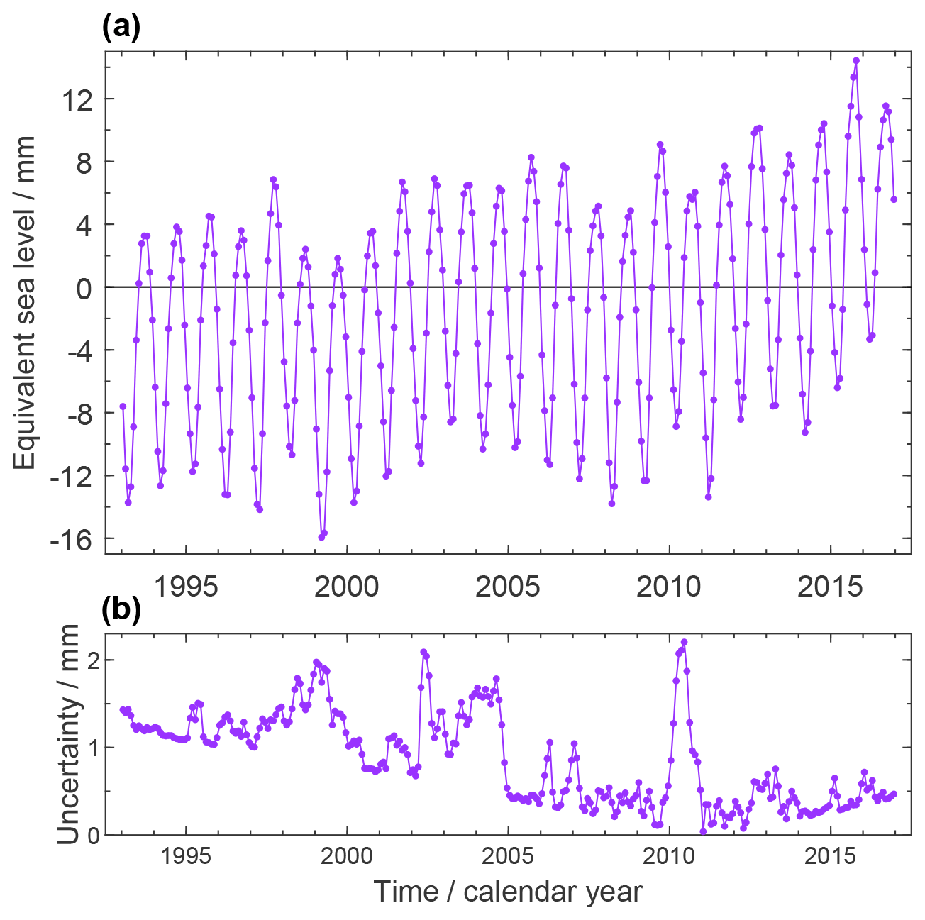
Figure 8(a) Contributions from global land water storage changes (except for Greenland and Antarctica) to GMSL, assessed by the WaterGAP global hydrology model at its monthly resolution. Water mass change is expressed in terms of equivalent GMSL change with respect to the mean of the reference interval of 2006–2015. (b) Uncertainties assessed for the estimates in (a).
3.7.2 Uncertainty assessment
Uncertainties are characterised by the spread between the four model runs. For each month, the standard deviation of the values from the four time series was taken as the standard uncertainty. Figure 8b shows these time-variable uncertainties of the LWSA. They reflect month-to-month differences in the spread between the ensemble members. Since the LWS anomalies referred to the 2006–2015 mean value and the four ensemble members show different trend, the uncertainty is lowest around 2011.0 and tends to increase towards the beginning (1993) and the end (2016). The standard deviation of the linear trends calculated for each ensemble member was taken as the standard uncertainty of the linear trend of the ensemble mean.
3.8 Other contributions and issues
Caspian Sea water storage changes are not included in the WaterGAP model domain and are therefore not included in our GMSL budget assessment. WCRP Global Sea Level Budget Group (2018) quotes this contribution as 0.075 ± 0.002 mm yr−1 since 1995 and 0.109 ± 0.004 mm yr−1 since 2002. Based on GRACE analyses, Cáceres et al. (2020) estimate the contribution to be 0.066 ± 0.003 mm yr−1 over 2003–2016, very similar to the GRACE-based estimate by Loomis and Luthcke (2017), which corresponds to 0.067 ± 0.007 mm yr−1 sea-level equivalent over 2003–2014.
Antarctic peripheral glaciers are included neither in the altimetry-based assessment of the Antarctic ice-mass change nor in the GGM assessment. The GRACE-based estimate for Antarctic ice-mass changes was designed to address the ice sheet proper but includes part of the mass changes of peripheral glaciers as a result of the low-spatial-resolution capability of satellite gravimetry. Gardner et al. (2013) estimate the Antarctic peripheral glaciers mass loss over 2003–2009 to a value equivalent to 0.017 ± 0.028 mm yr−1 GMSL. Zemp et al. (2019) estimate a loss over 2006–2016 at a value equivalent to 0.04 ± 0.30 mm yr−1 GMSL.
Changes in atmospheric water content (mainly tropospheric water vapour) are not included in our assessment. The atmosphere stores around 12 700 Gt of water (Trenberth, 2014) or 35 mm sea-level equivalent. Hartmann et al. (2013) report that the rate of change of tropospheric water vapour content is very likely consistent with the Clausius–Clapeyron relation (about a 7 % increase in water content per Kelvin). This corresponds to an equivalent GMSL effect on the order of −0.03 to −0.05 mm yr−1, which was also obtained by Dieng et al. (2017) from ERA-Interim atmospheric reanalysis results. Interannual variations of atmospheric water content reported by Dieng et al. (2017) are up to the order of 1 mm GMSL equivalent.
The elastic deformation of the ocean bottom induced by the present-day global redistribution of water and ice loads is not accounted for in our GMSL estimate from satellite altimetry (cf. Sect. 2.1). Since the deformation is downward on average over the global ocean, this omission leads to an underestimation of relative GMSL rise. Frederikse et al. (2017) estimated the effect for the period 1993–2014 to be 0.13 mm yr−1 for the global ocean and 0.17 mm yr−1 for the domain bounded by ±66∘ latitude, with higher rates in the second half of the period. Vishwakarma et al. (2020) estimated the effect for 2005–2015 to be 0.11 ± 0.02 mm yr−1 for a global altimetry domain buffered along the coasts.
Our conversion from OMC (or ocean-mass contributions) to sea-level change adopts the density of freshwater. In previous studies, either the density of freshwater or the density of seawater has been adopted, where both approaches have their justification (cf. Gregory et al., 2019; Vishwakarma et al., 2020). If we had adopted the seawater density (1028 kg m−3), our assessments of mass contributions would be reduced by 2.7 %.
We evaluate the OMB according to Eq. (5). We do the assessment for the P2 period (January 2003–August 2016; cf. Sect. 2.2). We use the OMC assessment made for the global ocean.
4.1 Linear trend
For the elements of the mass budget, we calculated linear trends over P2. We assessed their uncertainties as explained in Sect. 2.3 and specified for every element in Sect. 3. The results are shown in Table 3.
Table 3Linear trends of the mass budget elements (millimetre equivalent of global mean sea level per year) for the interval P2 and their standard uncertainties. Columns (a) and (b) adopt alternative estimates of the mass contributions from Greenland and Antarctica (as indicated by line labels and footnotes), while adopting the same estimates for the other budget elements.
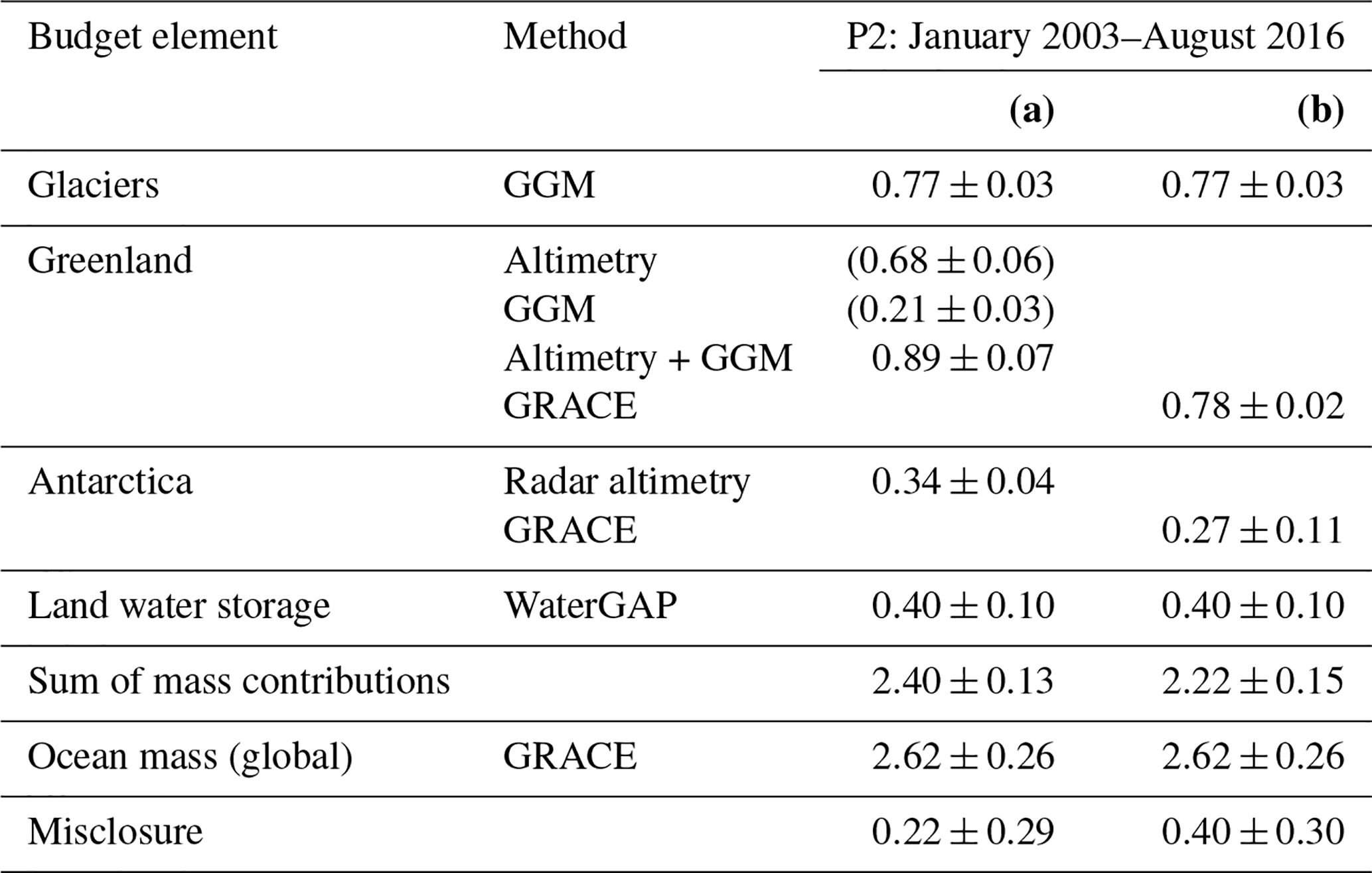
(a) Using altimetry-based estimates for Greenland and Antarctica complemented by GGM for Greenland peripheral glaciers. (b) Using GRACE-based estimates for Greenland and Antarctica.
All components exhibit a significant positive trend, i.e. water mass loss on land. Greenland ice masses contribute 0.78 ± 0.02 mm yr−1 as assessed from GRACE or 0.89 ± 0.07 mm yr−1 as assessed from radar altimetry for the ice sheet and from the GGM for the peripheral glaciers. The glaciers outside Greenland and Antarctica contribute 0.77 ± 0.03 mm yr−1, similar to Greenland. The Antarctic Ice Sheet's contribution is 0.27 ± 0.10 mm yr−1 if assessed from GRACE and 0.34 ± 0.04 mm yr−1 if assessed from radar altimetry. The trend in land water storage amounts to 0.40 ± 0.10 mm yr−1.
The sum of components is 2.19 ± 0.15 and 2.40 ± 0.13 mm yr−1, respectively, if the Greenland and Antarctica contributions are assessed using either GRACE or altimetry. The corresponding trend in mean global ocean mass according to our preferred GRACE-based solution (ITSG-Grace2018, GIA correction according to Caron et al., 2018) amounts to 2.62 ± 0.26 mm yr−1.
The misclosures of Eq. (5) with combined standard uncertainties are 0.40 ± 0.30 mm yr−1 (if using GRACE for Greenland and Antarctica) and 0.22 ± 0.29 mm yr−1 (if using altimetry in Greenland and Antarctica). Hence, the misclosure is at 1.5 times the standard uncertainty and 0.76 times the standard uncertainty, respectively. The mass budget is closed within standard uncertainty in the second case and still within the 1.65σ range (corresponding to the 90 % confidence range) in the first case.
4.2 Seasonal component
The inherent monthly resolution of GRACE-based OMC, GRACE-based AIS, and GrIS mass changes and modelled LWS and glacier mass changes allows us to analyse the budget of the seasonal variations of ocean mass. For this purpose, we analyse the annual cosine and sine amplitudes a3 and a4 of Eq. (3) just in the way we analysed the linear trend a2 in Sect. 4.1.
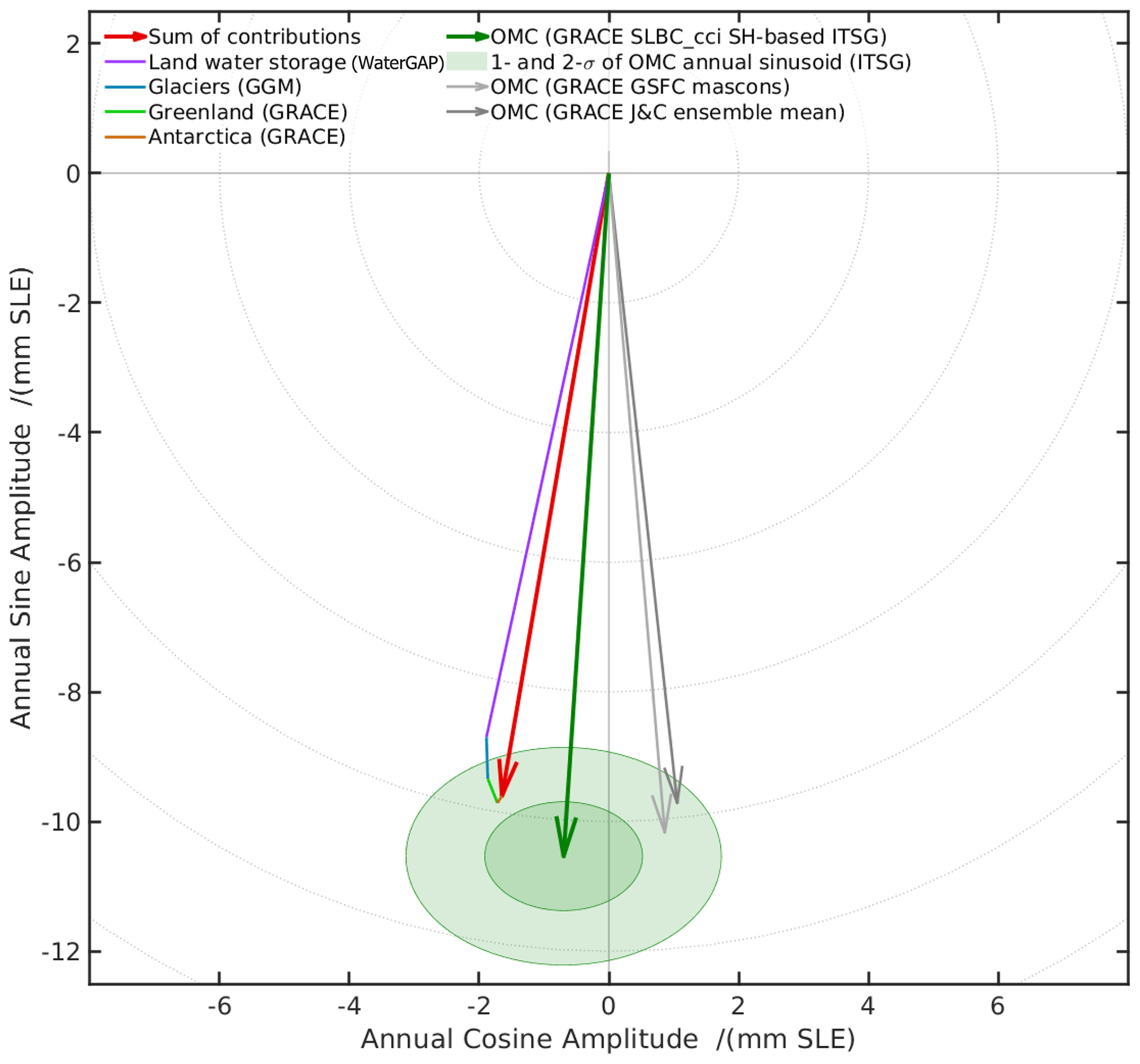
Figure 9Phase diagram of annual sine and cosine amplitudes of elements of the ocean-mass budget. Bold red vector: sum of contributions (using GRACE-based estimates for Greenland and Antarctica). Coloured thin lines: individual contributions (see legend). Bold dark-green vector: GRACE ocean-mass change (OMC) SLBC_cci solution based on GRACE ITSG-Grace2018, together with uncertainty ellipses. Thin grey vectors: external GRACE OMC solutions (GSFC mascons and Johnson and Chambers – J&C – ensemble mean). The phase difference between the red and the dark-green vector corresponds to 6 d.
Figure 9 shows the results of this analysis. The seasonal amplitudes of GRACE-based OMC and the sum of assessed contributions are very similar at 10.6 and 9.7 mm, respectively. LWS, with an amplitude of 8.9 mm, is by far the dominant source of seasonal OMC. The phase of GRACE OMC is approximately 6 d later than the phase of the sum of components. This small offset of phase is close to the 1σ uncertainties assessed for the GRACE OMC results, even though the uncertainty assessment was limited to effects of degree-one, C20, and leakage. Errors in the seasonal components of WaterGAP are another potential source of the phase offset.
The result does not change significantly (by less than 0.2 mm SLE – sea-level equivalent – for the annual cosine and sine amplitudes) if we replace the WaterGAP ensemble mean by one of the individual WaterGAP model runs or if we replace the ITSG-based GRACE OMC solutions by the CSR-based, GFZ-based, or JPL-based SH OMC solution generated by the SLBC_cci project. The phase offset between GRACE OMC and the sum of contributions becomes larger if we replace the SLBC_cci OMC solutions by the Johnson and Chambers SH-based OMC solutions or the GSFC mascon solutions (cf. specifications in Sect. 3.3); see grey arrows in Fig. 9.
4.3 Monthly time series
Figure 10 illustrates the monthly sampled time series of the elements of the OMB. The seasonal signal component, represented by annual and semi-annual harmonic functions was subtracted. The GRACE OMC (dark-green line) and the sum of components (dark-red line or light-red line) not only have similar trends (cf. Sect. 4.1) but also reflect interannual variations coherently. These interannual variations overlay the long-term trend and reach amplitudes of 2–3 mm. Clearly, they are dominated by the LWS contribution. They include a minimum in 2007/2008, a maximum in 2010, with a subsequent decrease to a minimum in 2011 related to a La Niña event (Boening et al., 2012). The sequence continues with an interannual maximum in 2012/2013, a minimum in 2013/2014, and another maximum in 2015/2016.
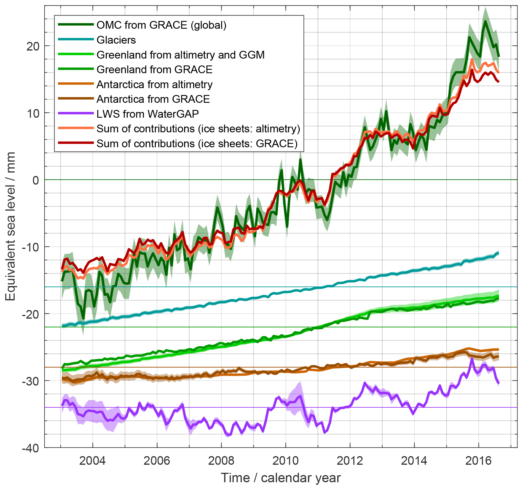
Figure 10Time series of the elements of the ocean-mass budget in January 2003–August 2016. See legend for attribution of graphs. The GRACE-based time series and the Antarctic altimetry time series were interpolated to monthly sampling. Seasonal variations are subtracted. Each graph shows anomalies with respect to a mean value over 2006–2015. Graphs are shifted arbitrarily along the ordinate axis. Transparent bands show standard uncertainties (except for the red sum-of-contribution graphs).
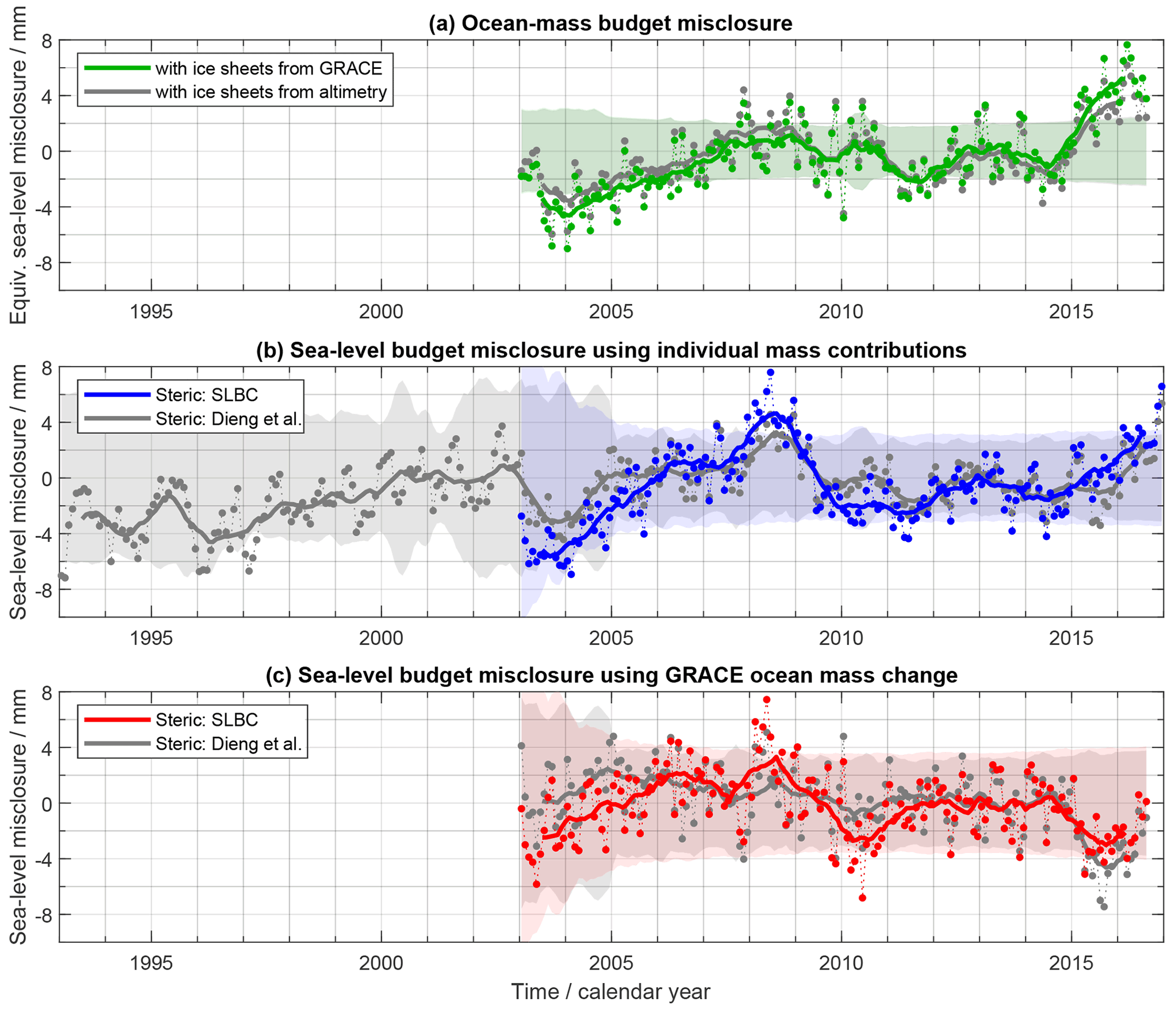
Figure 11(a) Ocean-mass budget misclosure (GRACE-based OMC minus the sum of assessed contributions) for the time series of monthly anomalies of mass budget elements as shown in Fig. 10. Dots: monthly misclosure for the case of GRACE-based (green) and altimetry-based (grey) ice sheet assessments. Thick lines: running 12-month mean, for better visibility of interannual features. Shaded bands (green and grey, almost identical in the figure): combined standard uncertainty (1σ) of the monthly misclosure. (b) Sea-level budget misclosure (GMSL minus the sum of contributions) for the time series shown in Fig. 12 using the individual mass contributions (involving the altimetry-based ice sheet assessments). Dots, lines, and shaded areas have the same meanings as in panel (a). Blue and grey: results employing the SLBC_cci steric data product and the Dieng et al. (2017) ensemble mean dataset, respectively. (c) Same as panel (b) but with application of GRACE-based OMC, instead of the sum of assessed mass contributions. Red and grey: results employing the SLBC_cci steric data product and the Dieng et al. (2017) data product, respectively.
Figure 11a shows the OMB misclosure, together with the combined standard uncertainties of all elements of Eq. (5). The percentages of monthly misclosure values within the 1σ, 2σ, 3σ, and 4σ combined uncertainty amount to 58.5 %, 92.7 %, 99.4 %, and 100.0 % for the time series using the GRACE-based ice sheet assessment. Similarly, the percentages are 64.0 %, 95.1 %, 100.0 %, and 100.0 % for the time series using the altimetry-based ice sheet assessments. These statistics support the realism of the uncertainty assessment where under the assumption of a Gaussian error distribution one would expect 67.3 %, 95.5 %, 99.7 %, and 99.99 % of the values to be within the 1σ, 2σ, 3σ, and 4σ limits, respectively.
We consider the two time periods P1 (altimetry era) and P2 (GRACE–Argo era) as introduced in Sect. 2.2. We concentrate on the steric product generated within SLBC_cci (see Sect. 3.2) when analysing the SLB over P2. For P1, which is not fully covered by the SLBC_cci steric product, we resort to the ensemble mean steric product updated from Dieng et al. (2017). The GRACE-based OMC estimates used here are those evaluated for the ocean between 65∘ N and 65∘ S. While for the present results of GRACE OMC this makes little difference, it is consistent to the averaging area of GMSL and the steric component.
5.1 Linear trend
Linear trends for the elements of the SLB for the two time periods are given in Table 4. The trends were calculated as explained in Sect. 2.2, and uncertainties were assessed as explained in Sect. 2.3 and specified for every element in Sect. 3.
Table 4Linear trends of the sea-level budget elements (millimetre equivalent of global mean sea level per year) for the intervals P1 (column a) and P2 (columns b, c, d) and their standard uncertainties. Different columns adopt alternative estimates of some of the budget elements (as indicated by line labels and footnotes), while adopting the same estimates for other elements. The estimates of total sea level, the steric contribution, and the GRACE-based OMC refer to the ocean between 65∘ N and 65∘ S, thereby excluding polar and subpolar oceans in the Arctic and the Southern Ocean.
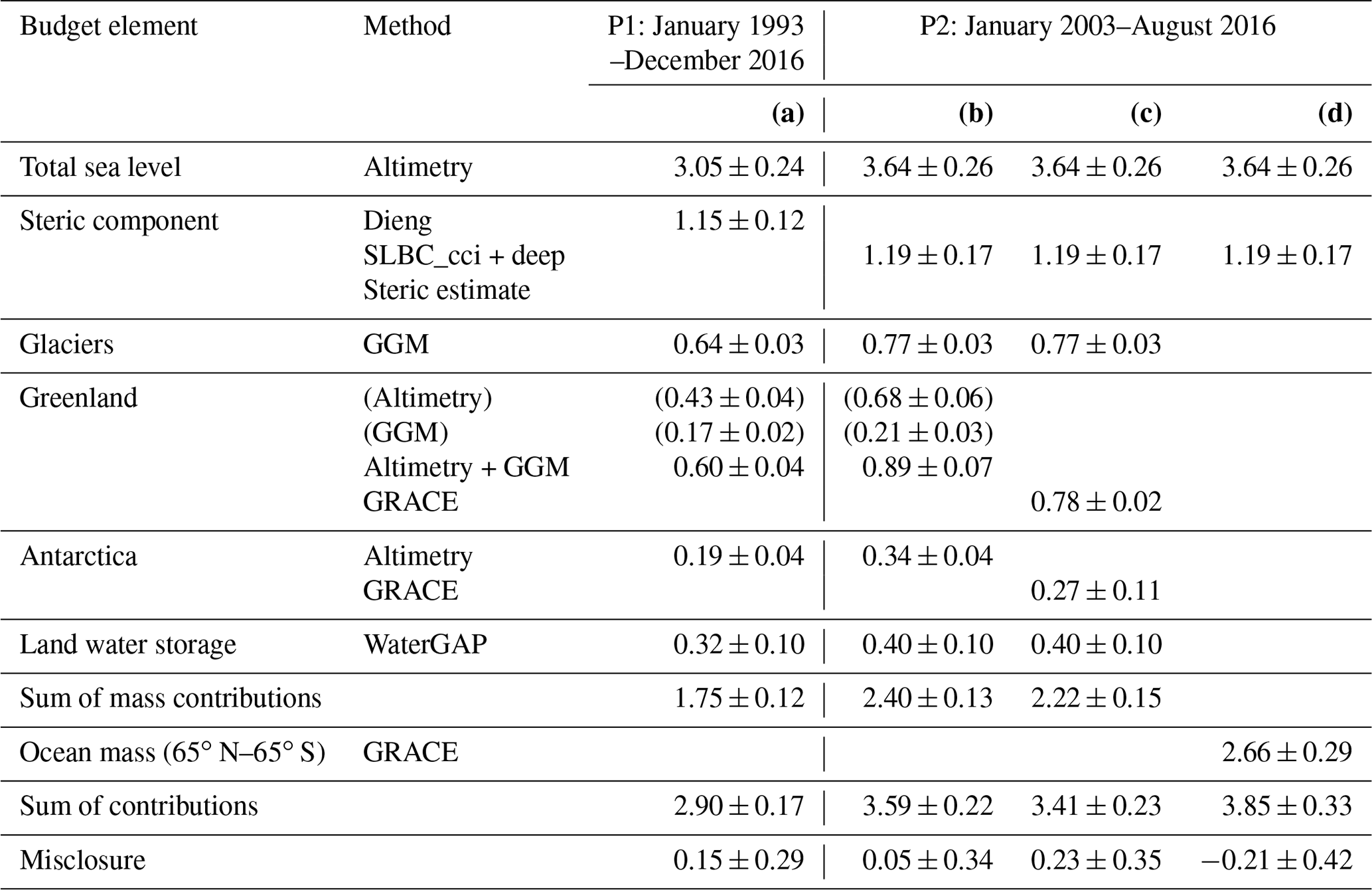
(a) Using the ensemble mean assessment of the steric contribution updated from Dieng et al. (2017) and using individual mass contribution estimates, where the Greenland and Antarctic contribution is assessed from altimetry, complemented by GGM for the Greenland peripheral glaciers. (b) Using the SLBC_cci steric product, complemented by the deep-ocean steric estimate, and using individual mass contribution estimates, where the Greenland and Antarctica contributions are assessed from altimetry, complemented by GGM for the Greenland peripheral glaciers. (c) Using the SLBC_cci steric product, complemented by the deep-ocean steric estimate, and using individual mass contribution estimates, where the Greenland and Antarctica contributions are assessed from GRACE. (d) Using the SLBC_cci steric product, complemented by the deep-ocean steric estimate, and using the GRACE-based OMC estimate.
For P1, the observed GMSL trend is 3.05 ± 0.24 mm yr−1. The sum of individual SLBC_cci v2 components is 2.90 ± 0.17 mm yr−1. This leaves a misclosure of 0.15 ± 0.29 mm yr−1.
For P2, the observed GMSL trend is 3.64 ± 0.26 mm yr−1. The sum of contributions is 3.85 ± 0.33 mm yr−1 if OMC is estimated from GRACE. The sum of contributions is 3.59 ± 0.22 and 3.41 ± 0.23 mm yr−1, if the mass contributions are assessed individually, involving altimetry-based estimates or GRACE-based estimates, respectively, for the ice sheets. The three choices of assessing OMC leave misclosures of −0.21 ± 0.42, 0.05 ± 0.34, and 0.23 ± 0.35 mm yr−1, respectively. The trend misclosures are hence within the standard uncertainty arising from the combined uncertainties of the involved budget elements.
If we used the Dieng et al. (2017) ensemble mean steric product for the P2 SLB assessment, the trend misclosure remained unchanged, since the steric trend over P2 is equally 1.19 mm yr−1 for the two alternative steric products.
The strong limitations of Argo coverage in the years before 2005 are reflected in the uncertainties of the SLBC_cci steric product (Fig. 3). Since the trend calculation accounts for these uncertainties (cf. Sect. 2.2), the SLBC_cci steric trend is dominated by the data starting in 2005. An alternative accounting for the large pre-2005 uncertainties would be to start the entire SLB assessment from 2005. For an alternative period, January 2005–August 2016, the trend budget is given in Table A1 (Appendix). For this period, the assessed linear trends of GMSL, the steric component, and the mass component are higher, by about 0.16, 0.07, and 0.17–0.29 mm yr−1, than for P2. The conclusions on the budget closure within uncertainties remain unchanged.
5.2 Monthly time series
For P1 (altimetry era) our SLB assessment refers to the Dieng et al. (2017) ensemble mean steric product and to the mass component composed from the individual contributions (involving altimetry-based assessments for the ice sheets). Figure 12 shows the monthly time series of the SLB elements. The seasonal signal component is removed. Apart from showing similar linear trends (cf. Sect. 5.1), the observed GMSL (black curve) and the sum of contributions (light-red curve) exhibit largely coherent interannual variations in the second half of P1 starting in 2005. These interannual variations, overlaid on the long-term trend, reach about 3–4 mm amplitudes. As a prominent feature, the La Niña-related local GMSL minimum in 2011 (Boening et al., 2012) arises as a superposition of synchronous variations of an LWS effect and a steric effect.
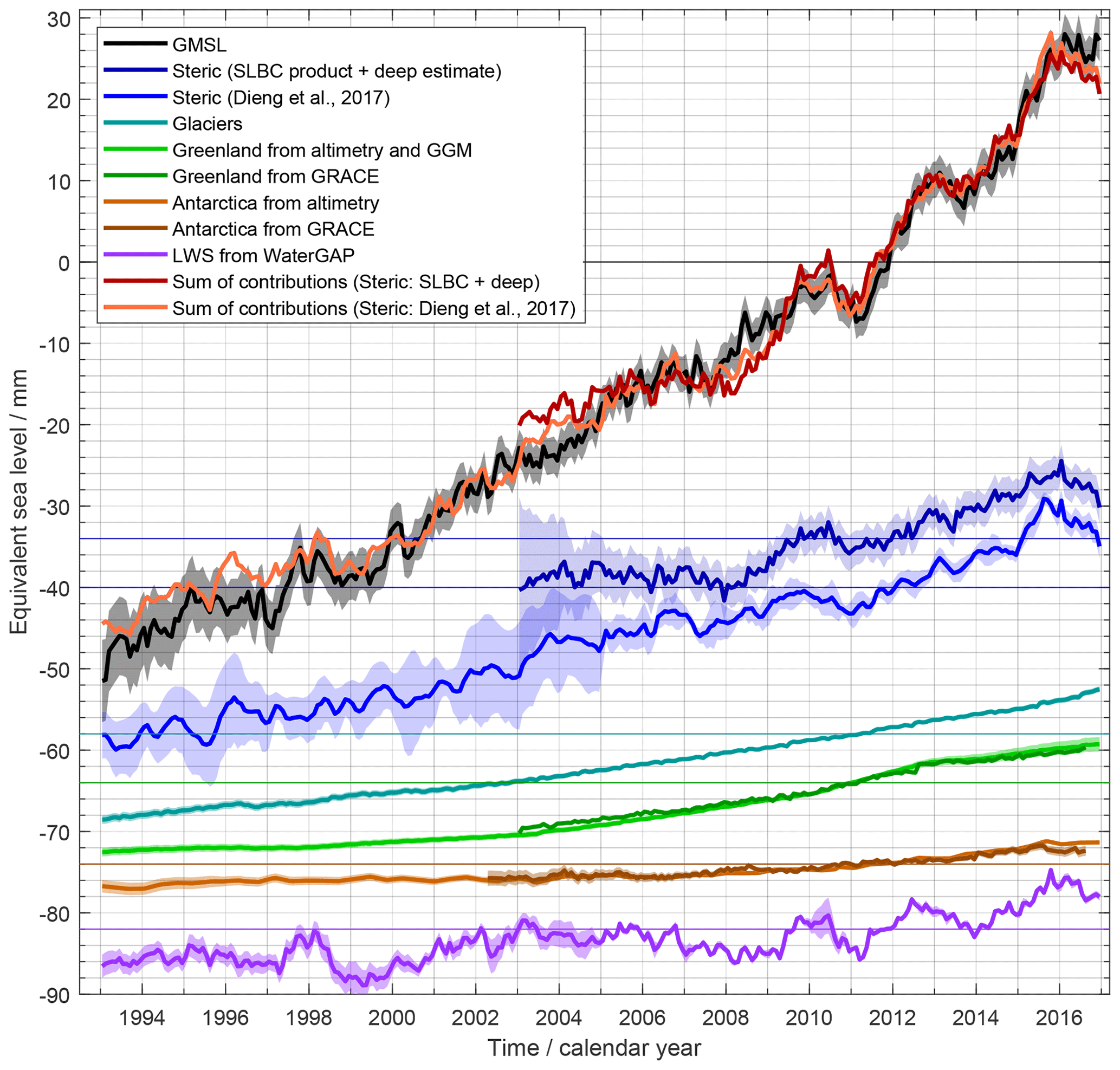
Figure 12Time series of SLB elements involving the individual contributions to ocean-mass change. See legend for attribution of graphs. The sum-of-components graphs use altimetry-based ice sheet assessments. The GRACE-based time series and the Antarctic altimetry time series were interpolated to monthly sampling. Seasonal variations are subtracted. Each graph shows anomalies with respect to a mean value over 2006–2015. Graphs are shifted arbitrarily along the ordinate axis. Standard uncertainties are shown by transparent bands (except for the sum-of-contribution graphs).
The associated misclosure time series are shown in Fig. 11b (in grey). Deviations between GMSL and the sum of components are relatively large in the early years of 1993–1996. In this period GMSL uncertainties are large (cf. Fig. 1b) due to uncertainties of the TOPEX-A drift correction. In addition, the steric component has large uncertainties in this period and further through 2004, where it is based on XBT (expendable bathythermograph) data and therefore suffers from sparse coverage both geographically and at depth (below 700 m). The monthly misclosure values for P1 are within the 1σ and 2σ uncertainty band, respectively, for 90.9 % and 100.0 % of the months. Hence, the distribution is narrower than expected from the uncertainty assessment under the assumption of a Gaussian error distribution.
For P2 (GRACE–Argo era) the SLB analysis may employ the SLBC_cci steric dataset, which is also shown in Fig. 12. Again, interannual variations of GMSL (black curve) and the sum of components (dark-red curve) agree largely in their sequence of positive and negative deviations from a long-term evolution, with the exception of the early Argo years of 2003 and 2004. Figure 11b shows (in blue) the misclosure of the SLB when using this SLBC_cci steric dataset (and the individual mass contribution assessments). The percentage of misclosures within the 1σ, 2σ, and 3σ ranges of combined uncertainties are 84.8 %, 99.4 %, and 100.0 %, respectively, indicative, again, of a narrower distribution than allowed for by the assessed uncertainties.
For the case of using the GRACE-based OMC, the monthly budget assessment over P2 is illustrated in Fig. 13. While the use of GRACE OMC introduces more month-to-month noise into the sum-of-components time series than the use of individual mass contributions, the features of interannual variations discussed above are again coherently reflected in the GMSL and the sum of contributions. The related monthly misclosure time series are shown in Fig. 11c. When using the SLBC_cci steric product, the monthly misclosure values are within the 1σ, 2σ, and 3σ range, respectively, for 89.6 %, 99.4 %, and 100.0 % of the months, again far within the assessed combined error distribution
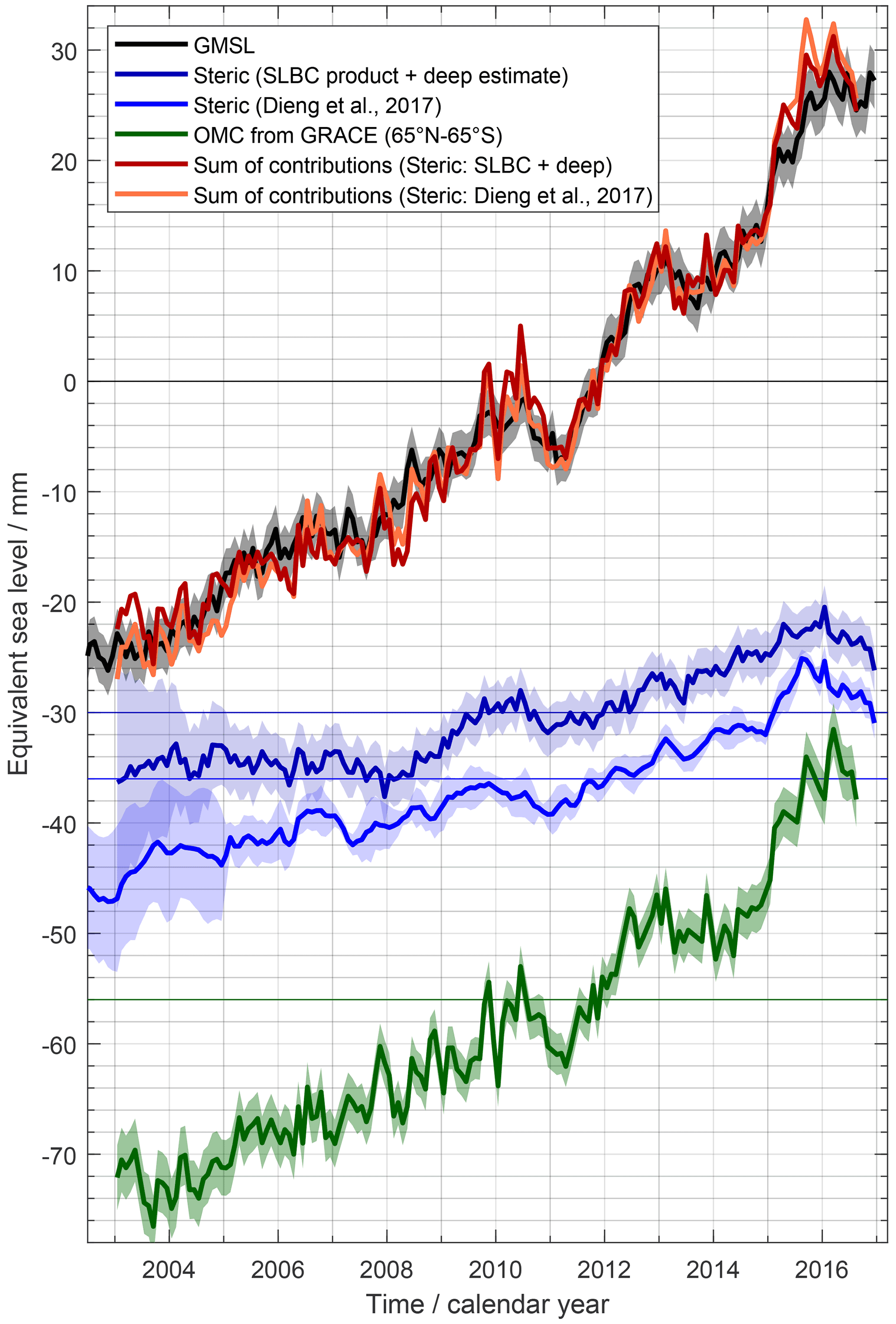
Figure 13Time series of SLB elements involving the GRACE-based assessment of ocean-mass change. See legend for attribution of graphs. The GRACE-based time series were interpolated to monthly sampling. Seasonal variations are subtracted. Each graph shows anomalies with respect to a mean value over 2006–2015. Graphs are shifted arbitrarily along the ordinate axis. Standard uncertainties are shown by transparent bands (except for the sum-of-contribution graphs).
We cannot attribute the misclosures in the budgets of linear trends to any particular error source, as the uncertainties on the order of 0.2 to 0.3 mm yr−1 in various elements of the OMB and SLB would make such an attribution extremely ambiguous. In contrast, for the interannual features in the misclosure time series of the different budgets (Fig. 11) we can suggest indications on misclosure origins by comparing them among each other and with the interannual variations of the budget elements. Interannual variations are depicted as variations of the running annual means of the misclosure time series, shown as bold curves in Fig. 11.
The OMB misclosure varies interannually between roughly −2 and +2 mm (bold curves in Fig. 11a). The SLB misclosure varies interannually between roughly −6 and +4 mm (bold curves in Fig. 11b, c) depending on which steric product and which way of estimating OMC are used. Errors of the datasets on GMSL, the steric contribution, GRACE-based OMC, and LWS are most likely responsible for these interannual misclosures. The glacier and ice sheet time series involve relatively small interannual variations (cf. Fig. 12) so that their errors are unlikely to exceed the sub-millimetre level. The unassessed contribution of atmospheric water content (cf. Sect. 3.8) could contribute to the misclosure, though.
As a starting point, we discuss the SLB misclosure obtained if estimating the steric contribution by the SLBC_cci steric product and estimating the mass component by the sum of mass contributions (Fig. 11b, blue curve). As a first feature, the misclosure moves from −6 to 0 mm between mid-2003 and mid-2006, indicating that over this 3-year period the sum of contributions rose 2 mm yr−1 less than the altimetry-based GMSL. At least part of this feature is readily explained by the limitations of the SLBC_cci steric product in these early years of the Argo system, as discussed in Sect. 3.2.
As a second prominent feature, the misclosure rises by 4 mm from 2006 to 2008 and falls again by 6 mm from 2008 and 2010. From Fig. 12 we see that this misclosure is related to the sum of components suggesting a temporary slowdown of sea-level rise from 2006 to 2008, while the altimetric GMSL exhibits less of such a slowdown. The SLBC_cci steric time series (Figs. 3, 12) has a feature of fall and rise by 3–4 mm in those 2006–2008 and 2008–2010 periods, and this feature enters the SLB misclosure with negative sign. In addition, the mass budget misclosure (Fig. 11a) has a similar rise and fall by 1 to 2 mm in the same 2006–2008 and 2008–2010 periods. Replacing the individual mass components by GRACE-based OMC reduces the misclosure feature (compare the blue line of Fig. 11b and red line of Fig. 11c). Replacing the SLBC_cci steric product by the Dieng et al. (2017) ensemble mean steric time series further reduces this feature (compare the red line and grey line of Fig. 11c). This may suggest that between 2006 and 2010 the interannual variations of OMC and the steric component are more accurately represented by GRACE-based OMC and the Dieng ensemble mean, respectively, than by the sum of mass contributions involving modelled LWS and the SLBC_cci steric product.
7.1 Budget closure and uncertainties
The six budget assessments we made for linear trends (two OMB assessments for P2, one SLB assessment for P1, and three SLB assessments for P2; cf. Tables 3 and 4) revealed misclosure within the 1σ range in five cases and at 1.5σ in one case. Hence, misclosures are compatible with assessed uncertainties. Assessed uncertainties of the trends of various budget elements are on a similarly high level. For example, for P2 the trend uncertainties are 0.26 mm yr−1 for GMSL, 0.17 mm yr−1 for the steric component, and 0.13 to 0.29 mm yr−1 for the mass component, depending on how it is assessed.
As a consequence of the budget closure within uncertainties, no significant estimates of missing budget elements can be made based on the present budget assessments. Likewise, the linear trend of any single component cannot be easily validated through budget considerations. In cases where the budget of trends is closed much better than the combined uncertainties (e.g. column b in Table 4), this could just result from an incidental compensation of errors in the involved budget elements. It may be interesting to illustrate this notion by the history of the present study. Updates of the GRACE OMC analysis with respect to a previous version (cf. Sect. 3.3) shifted the misclosures of OMB (Table 3) and SLB (Table 4d). Picking OMC solution variants that provide near-zero budget closure would have led to different choices prior to and after the update. However, the methodological developments neither for GRACE OMC estimates nor for estimates of the other budget elements are concluded by far.
Our estimates of ice sheet contributions used the data products from the two methods (satellite gravimetry and satellite altimetry) exploited by the AIS CCI project and the GrIS CCI project. The input–output method (IOM, e.g. Rignot et al., 2019) not used here has resulted in estimates of stronger losses, in particular for the AIS. Rignot et al. (2019) reported an AIS mass loss at 168.9 ± 5 Gt yr−1 (or 0.47 ± 0.01 mm yr−1 sea-level equivalent) over 1992–2017, a period similar to our P1, where we estimate 0.19 ± 0.04 mm yr−1 sea-level equivalent. Therefore, using IOM-based estimates like those by Rignot et al. (2019) would likely result in less positive or slightly negative misclosures of the OMB and SLB as compared to our assessments in Tables 3a and b and 4a, b, and c. Again, since the budgets are closed within uncertainties for any of the discussed ice sheet estimates, we cannot use our budget assessments to judge which of the discrepant AIS estimates is more correct.
The trends of the individual budget components assessed here for P1 and P2 agree (with two exceptions) within stated uncertainties with the assessment by the IPCC SROCC (Oppenheimer et al., 2019, Table 4.1) for the similar (though not equal) periods of 1993–2015 and 2006–2015, respectively. As one exception, our GRACE-based OMC estimate (2.62 ± 0.26 mm yr−1 for P2, 2.83 ± 0.29 mm yr−1 for January 2005–August 2016) exceeds the one of the IPCC SROCC (2.23 ± 0.16), which is based on an ensemble mean from WCRP Global Sea Level Budget Group (2018) and has a considerably smaller uncertainty estimate than ours. The difference is associated with updates of standards on the treatment of degree-one and C20 since the time of WCRP Global Sea Level Budget Group (2018) (see our discussion at the end of Sect. 3.3) and with our use of the Caron et al. (2018) GIA correction (cf. Table 1). A second disagreement with the IPCC SROCC concerns the LWS contribution. The SROCC reported a negative sea-level contribution at −0.21 mm yr−1 for 2006–2015 based on GRACE analyses, while our WaterGAP results indicate a positive contribution at 0.65 mm yr−1 for 2006–2015 (0.40 mm yr−1 for P2). However, a new GRACE-based assessment of continental mass change (Cáceres et al., 2020, updated by Gutknecht et al., 2020) corrected for the GGM-based glacier mass trend also determines a positive LWS contribution at 0.31 mm yr−1 for 2006–2015 (0.42 mm yr−1 for P2). This is also consistent with another GRACE assessment by Kim et al. (2019). Assessing the LWS contribution to GMSL remains a challenge.
More recently, the IPCC Sixth Assessment Report (AR6, Fox-Kemper et al., 2021) incorporated our assessment (Cáceres et al., 2020) and the one by Frederikse et al. (2020) to quote a LWS GMSL contribution that is now positive for both 1993–2018 and 2006–2018. Overall, the AR6 assessment of all budget elements for 1993–2018, as well as the assessment by Frederikse et al. (2020) for the same period, agree with our results for P1 within uncertainties. As a single exception, AR6 assessed a lower Greenland contribution than we do. Reasons may include the non-uniform treatment of peripheral glaciers by Shepherd et al. (2019), which underlies the AR6 Greenland assessment, as well as the difference between the time periods considered.
Our analysis of the OMB and the SLB on a time series basis exploits the intrinsic monthly resolution of almost all budget elements. Only for the altimetry-based GrIS and AIS assessments is true month-to-month variability not contained in the time series interpolated to monthly resolution. We found that the spread of monthly misclosure of OMB and of SLB is similar to, or narrower than, a Gaussian distribution with a standard deviation equal to the combined standard uncertainties of the budget elements.
7.2 Limitations of the study
While the uncertainty assessments made for the individual budget components were described in a common framework, different approaches to uncertainty characterisation were used for the different products. The reasons for the conceptual differences as well as their consequences for the relative uncertainty levels within the budget assessments have not been fully elaborated. A further consolidation and standardisation of uncertainty characterisation could allow, in a more flexible way, for propagating uncertainties to different functionals, such as to anomalies with respect to different reference states, or to time-dependent rates of change.
No correlation between errors of different budget elements was accounted for when combining the different elements in budget assessments. However, such correlations exist. An important example is the GIA correction, which is significant by its magnitudes and uncertainties. In our study, the GIA corrections and their uncertainties are −1.37 ± 0.19 mm yr−1 for the GRACE OMC estimate, −0.14 ± 0.09 and −0.02 ± 0.02 mm yr−1 for the GRACE-based assessment of the Antarctic and Greenland mass contribution, respectively, and −0.30 ± 0.05 mm yr−1 for the altimetric GMSL change. (These numbers are subtracted from the uncorrected results.) The errors in these GIA corrections to different budget elements are likely correlated among each other.
As a matter of fact, already the choice of a GIA model used for GIA corrections poses consistency issues not resolved in the present study. We used the regional GIA model IJ05_R2 (Ivins et al., 2013) for GRACE-based AIS mass change estimates as opposed to the global GIA models used for GRACE-based OMC estimates and GrIS mass change estimates. Subject to ongoing study is whether global models are consistent with geodetic and geological evidence over Antarctica (Ivins et al., 2013; Argus et al., 2014). Regional GIA models like IJ05_R2 and W12 (Ivins et al., 2013; Whitehouse et al., 2012), on the other hand, are not constructed to obey geological evidence on global sea-level history.
Other contributions (Sect. 3.8) which were included neither in our budget analysis nor in our uncertainty assessment are on the order of 0.1 mm yr−1, with the largest single unconsidered contribution likely being the elastic seafloor deformation effect. Coarse estimates based on the literature review of Sect. 3.8 indicate that considering the discussed effects does not change the overall conclusions of our study.
It is also important to mention that our assessment of the “global” mean sea level as well as our assessment of the steric contribution, by its limitation to the 65∘ N–65∘ S latitude range, left out 6 % of the global ocean area. In the Arctic and in the Southern Ocean, satellite altimetry has sampling limitations due to orbital geometry and sea-ice coverage. Likewise, Argo floats and other in situ sensors have sampling limitations due to the presence of sea ice. Therefore, SLB assessments for the polar oceans (e.g. Raj et al., 2020) are even more challenging than for the 65∘ N–65∘ S latitude range focussed on in this paper. An assessment of the truly global mean sea level and its contributions would involve higher uncertainties than quoted here for the 65∘ N–65∘ S range.
A compiled dataset of time series of the elements of the GMSL budget and of the OMB together with their uncertainties is freely available for download at https://doi.org/10.5285/17c2ce31784048de93996275ee976fff (Horwath et al., 2021). The version 2.2 dataset (ESACCI_SLBC_TimeSeriesOfSeaLevelBudgetElements_v2.2.csv) is an update of the previous version 2.1 dataset, where the update concerns the update of GRACE OMC estimates outlined in Sect. 3.3. The single file in CSV (comma-separated value) format contains the time series presented in Figs. 10, 12, and 13. These time series are all at an identical monthly sampling, resulting from interpolation of the original time series where necessary. Uncertainties were partly recalculated from the original data products (as described in Sect. 3) in order to make them consistently refer to anomalies with respect to the same reference interval of January 2006–December 2015 as stated in Sect. 2.3. Seasonal signals (according to Eq. 10) are removed from all time series.
This study assessed CCI data products related to the SLB; advanced the generation of new time series of SLB elements based on satellite Earth observation and modelling; and integrated, within a consistent framework, the products into an analysis of the OMB and the SLB. The consolidation, improvement, and exhibition (in Figs. 1, 3–8) of the uncertainty characterisation for every budget element were central to this study. The datasets and analyses presented here document both achievements and limitations identified within the SLBC_cci study.
9.1 Advances on data products on individual budget elements
For the GMSL, the use of the averaged ESA CCI 2.0 gridded sea-level data was enhanced by the incorporation of the uncertainty estimate over each GMSL time step from Ablain et al. (2019). Three major sources of errors were considered in the composition of a variance–covariance matrix to obtain GMSL uncertainty. The GMSL trend uncertainty over 1993–2016 (after correcting the TOPEX A drift) is assessed as 0.24 mm yr−1 (1σ).
For the steric-sea-level change, we developed a formal-uncertainty framework around the estimation of steric height from Argo profiles, including propagation to gridded and time series products. The framework includes simple models to estimate each uncertainty source and their error covariance structures. Global sampling uncertainty was included when obtaining the global mean from the gridded products. Inclusion of SST from SST CCI to condition the climatology of the mixed layer reduced bias of the steric change in the upper ocean, with a small beneficial impact. A full error covariance matrix was calculated for the global steric time series, facilitating robust calculation of linear trends and their uncertainties.
OMC was inferred from recent GRACE SH solution releases. The employed methodology is in the continuity of recent methodological developments and builds on comprehensive insights into the sensitivity to choices of input data and of the treatment of background models. The related uncertainty assessment accounted for this sensitivity.
For the glacier contribution, the introduction of an ensemble approach to reconstruct glacier mass change and the systematic multi-objective optimisation of the global model parameters led to results that generally confirm the previous estimates and which also agree well with methods based on observations only (Zemp et al., 2019). However, the increased model performance (higher correlation with observations on individual glaciers and better representation of the observed variance of mass balance) increased the confidence in the results.
For the GrIS contribution, we devised an empirical and effective way to convert the radar altimetry elevation changes into mass changes. The resulting time series was independently tested against the GRACE-derived time series, and it has shown very high compatibility.
For the AIS contribution, the new time series of Antarctic mass change from satellite radar altimetry is the result of an improved processing chain and a better characterisation of uncertainties. With a time-evolving ice and snow density mask and a new method for interpolating surface elevation change in areas located beyond the latitudinal limit of satellite radar altimeters and in between satellite tracks, we have provided an updated time series of Antarctic mass change from 1992 to 2017. This new dataset (cf. Shepherd et al., 2019) shows that ice losses are dominated by the Pine Island Glacier and Thwaites Glacier basins in West Antarctica, where mass losses (expressed as equivalent GMSL contribution) have increased from 0.04 ± 0.01 mm yr−1 in 1992–1997 to 0.36 ± 0.03 mm yr−1 in 2012–2017.
For the LWS contribution, the version of the global hydrological model WaterGAP (version 2.2d) was developed and applied, which includes the commissioning years of individual reservoirs to take into account increased water storage behind dams as well as regionalised model parameterisations to improve the simulation of groundwater depletion (Müller Schmied et al., 2021). Comprehensive insights into the model sensitivity to choices of irrigation water use assumptions and climate input data were acquired, enabling a first uncertainty estimation. The good fit of the simulated monthly total water storage anomaly (sum of land water storage and glacier storage) to GRACE-derived estimates, in particular regarding seasonality and deseasonalised long-term variability, enhanced the confidence in the simulated land water contributions (Cáceres et al., 2020).
9.2 Sea-level budget and ocean-mass budget
As summarised in Tables 3 and 4, the SLB and the OMB are closed according to their assessed uncertainties for their evaluation periods P1 (January 1993–December 2016, SLB) and P2 (January 2003–August 2016, SLB and OMB). We may reformulate the budgets as follows. The GMSL linear trend over P1 and P2 is 3.05 and 3.64 mm yr−1, respectively. The larger trend over P2 is due to an increased mass component, not only predominantly from Greenland but also from the other mass contributors. Over P1 (P2) the steric contribution is 38 % (33 %) of GMSL rise, while the mass contribution is 57 % (61 %–73 %). Among the sources of OMC, glaciers outside Greenland and Antarctica contributed 21 % (21 %) of total GMSL rise; Greenland contributed 20 % (21 %–24 %); Antarctica contributed 6 % (8 %–9 %); and LWS contributed 10 % (11 %). The SLB misclosure (GMSL minus the sum of assessed contributions) is between −6 % and +6 % of the GMSL rise. Ranges quoted here arise from different options of assessing the contributions. Uncertainties given in Tables 3 and 4 are not repeated here.
We cannot attribute the statistically insignificant misclosure of linear trends. We tentatively attributed interannual features of misclosure to errors in some of the involved datasets. When the SLBC_cci steric product is used, a SLB misclosure in the early years of Argo of 2003–2006 is likely due to an underestimation of the steric-sea-level rise associated with the global sampling error in conjunction with the constraints towards a static climatology, as discussed in Sect. 3.2.2. An interannual misclosure feature between 2006 and 2010 might be related to the SLBC_cci steric product and the WaterGAP model making the impression of a temporary slowdown in sea-level rise in 2006–2008 with subsequent recovery in 2008–2010, which is not as pronounced in the GMSL record.
9.3 Outlook
Future work will naturally include an extension of the considered time periods. It will be additionally spurred by the availability of new data types (Cazenave et al., 2019). GRACE-FO (Follow-On) launched in August 2018 already facilitates a satellite gravity times series spanning 19 years (yet with interruptions). It will be equally important to continue this time series beyond GRACE-FO as currently jointly considered by ESA and NASA for the next-generation gravity mission (Haagmans et al., 2020). The Deep Argo project (Roemmich et al., 2019) promises new observational constraints on deep-ocean steric contributions. With the Sentinel-6/Jason-CS (Continuity of Service) mission (Scharroo et al., 2016) the continuation of satellite altimetry in the 66∘ N–66∘ S latitude range is enabled with synthetic-aperture resolution capabilities exceeding those of pulse-limited altimeters. Continuity of precise satellite radar altimetry at high latitudes beyond CryoSat-2 still has to be ensured. Perspectives and requirements for long-term GMSL budget studies are detailed by Cazenave et al. (2019). Additional ECVs related to the global water and energy cycle call for their exploration in SLB studies. In the framework of ESA's CCI, results from Water Vapour CCI, Snow CCI, or Lakes CCI are among the candidates.
Limitations discussed in Sect. 7.2 call for further methodological developments. For example, the consideration of GIA as an independent element in SLB analyses could help to enforce its consistent treatment. This will be particularly important for regional SLB studies, since GIA is a driver of regional sea-level change and OMC. Such a treatment of GIA could be in accord with the treatment of elastic solid-Earth load deformations as proposed by Vishwakarma et al. (2020). Recent probabilistic characterisations of GIA model errors (Caron et al., 2018) allow for their propagation to error covariances of the SLB elements (cf. Frederikse et al., 2020).
While GMSL is an important global indicator, it is indispensable to monitor and understand the geographic patterns of sea-level change, that is, regional sea level. Regional sea level reflects the different processes causing sea-level change, which may be hidden in GMSL (e.g. Stammer et al., 2013; Hamlington et al., 2020). Understanding and projecting these processes, with implications down to coastal-impact research, is the ultimate goal. The further development of methodologies for regional SLB assessments and their application will be an important step towards this goal.
Table A1Same as the last three columns of Table 4 but for the alternative period of January 2005–August 2016, when the Argo network was fully established. Linear trends of the sea-level budget elements (millimetre equivalent of global mean sea level per year).
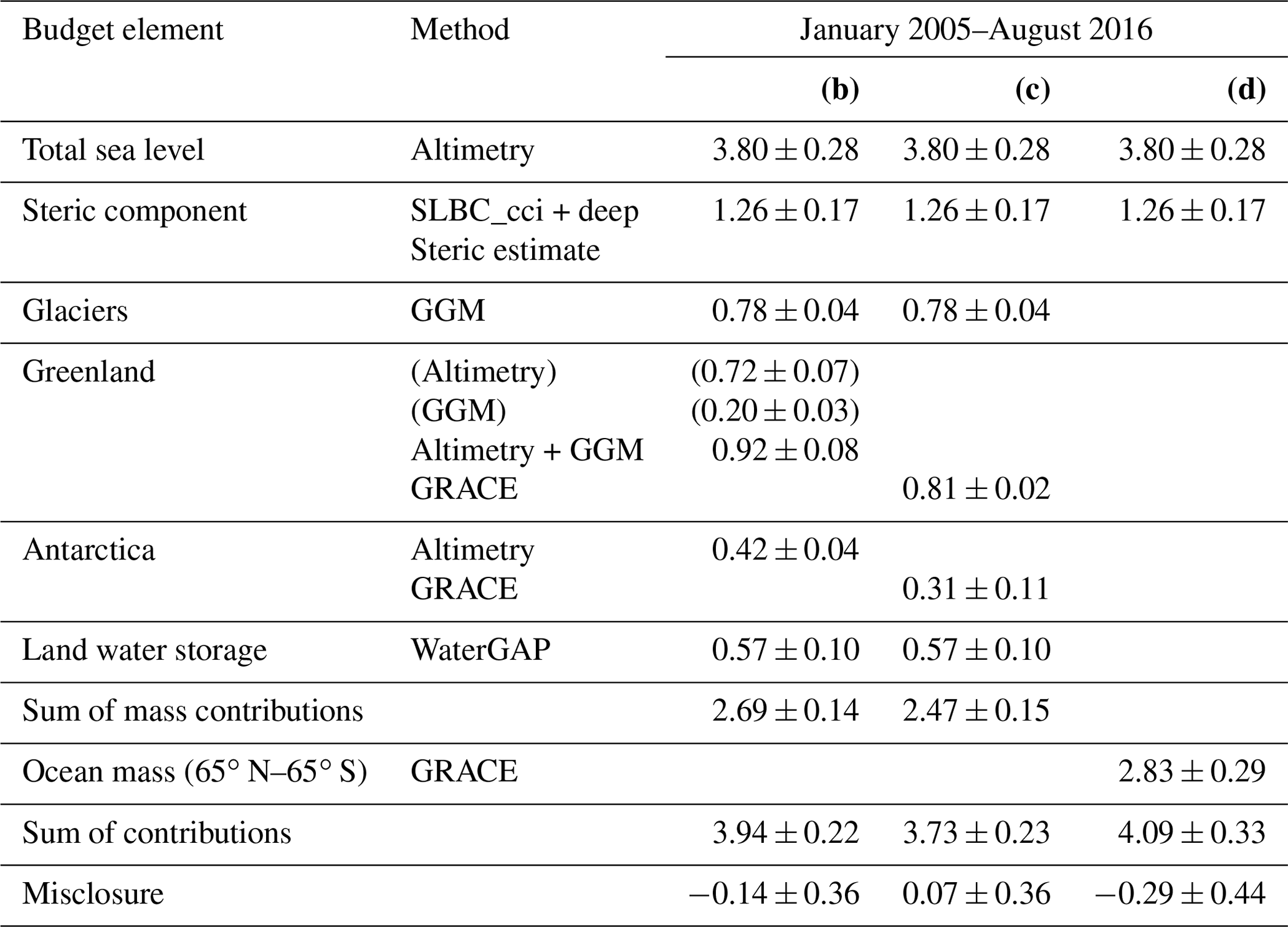
AC, JB, MH, AS, RF, CJM, JAJ, OBA, BM, FP, PD, and KN designed the study. MH led the study and the compilation and editing of the manuscript. AC, HKP, and FM contributed the GMSL dataset and its description. CJM, CRM, and KvS contributed the SLBC_cci steric dataset and its description. BDG contributed the GRACE-based OMC dataset and its description. BM contributed the global glacier dataset and its description. VRB and RF contributed the GRACE-based Greenland dataset and its description. LSS and SBS contributed the altimetry-based Greenland dataset and its description. AG and MH contributed the GRACE-based Antarctica dataset and its description. AEH, AS, and IO contributed the altimetry-based Antarctica dataset and its description. PD, DC, and HMS contributed the LWS dataset and its description. BDG conducted the ocean-mass budget analyses and drafted their description. HKP, AC, and MH conducted the sea-level budget analyses and misclosure attribution study and drafted their description. All authors discussed the results and contributed to the editing of the manuscript. KN managed the project administration. JB launched the ESA Sea Level Budget Closure CCI (SLBC_cci) project and, with the support of MR, supervised the development of this research activity and reviewed all the deliverables.
The contact author has declared that neither they nor their co-authors have any competing interests.
Publisher’s note: Copernicus Publications remains neutral with regard to jurisdictional claims in published maps and institutional affiliations.
This study was supported by the European Space Agency through the Sea Level Budget Closure Climate Change Initiative (CCI) project (contract no. 4000119910/17/I-NB). We thank the editor, Giuseppe Manzella, and the reviewers, Jianli Chen, Riccardo Riva, and an anonymous reviewer, as well as Jean-François Legeais, for their constructive and insightful comments which helped to improve this manuscript. We thank the German Space Operations Center (GSOC) of the German Aerospace Center (DLR) for providing continuous and nearly 100 % of the raw telemetry data of the twin GRACE satellites.
This research has been supported by the European Space Agency (grant no. 4000119910/17/I-NB).
This paper was edited by Giuseppe M. R. Manzella and reviewed by Jianli Chen, Riccardo Riva, and one anonymous referee.
A, G., Wahr, J., and Zhong, S.: Computations of the viscoelastic response of a 3-D compressible Earth to surface loading: an application to Glacial Isostatic Adjustment in Antarctica and Canada, Geophys. J. Int., 192, 557–572, https://doi.org/10.1093/gji/ggs030, 2013.
Ablain, M., Cazenave, A., Larnicol, G., Balmaseda, M., Cipollini, P., Faugère, Y., Fernandes, M. J., Henry, O., Johannessen, J. A., Knudsen, P., Andersen, O., Legeais, J., Meyssignac, B., Picot, N., Roca, M., Rudenko, S., Scharffenberg, M. G., Stammer, D., Timms, G., and Benveniste, J.: Improved sea level record over the satellite altimetry era (1993–2010) from the Climate Change Initiative project, Ocean Sci., 11, 67–82, https://doi.org/10.5194/os-11-67-2015, 2015.
Ablain, M., Legeais, J. F., Prandi, P., Marcos, M., Fenoglio-Marc, L., Dieng, H. B., Benveniste, J., and Cazenave, A.: Altimetry-based sea-level at global and regional scales, Surv. Geophys., 38, 7–31, https://doi.org/10.1007/s10712-016-9389-8, 2017a.
Ablain, M., Jugier, R., Zawadki, L., Taburet, N., Cazenave, A., and Meyssignac, B.: The TOPEX-A Drift and Impacts on GMSL Time Series, AVISO Website, October 2017, available at: https://meetings.aviso.altimetry.fr/fileadmin/user_upload/tx_ausyclsseminar/files/Poster_OSTST17_GMSL_Drift_TOPEX-A.pdf (last access: 13 January 2022), 2017b.
Ablain, M., Meyssignac, B., Zawadzki, L., Jugier, R., Ribes, A., Spada, G., Benveniste, J., Cazenave, A., and Picot, N.: Uncertainty in satellite estimates of global mean sea-level changes, trend and acceleration, Earth Syst. Sci. Data, 11, 1189–1202, https://doi.org/10.5194/essd-11-1189-2019, 2019.
Argus, D., Peltier, W., Drummond, R., and Moore, S.: The Antarctic component of glacial isostatic adjustment model ICE-6G_C (VM5a) based upon GPS measurements of vertical motion of the crust, exposure age dating of ice thickness variations and relative sea-level histories, Geophys. J. Int., 198, 537–563, https://doi.org/10.1093/gji/ggu140, 2014.
Bamber, J. L., Westaway, R. M., Marzeion, B., and Wouters, B.: The land ice contribution to sea-level during the satellite era, Environ. Res. Lett., 13, 063008, https://doi.org/10.1088/1748-9326/aac2f0, 2018.
Barletta, V. R., Sørensen, L. S., and Forsberg, R.: Scatter of mass changes estimates at basin scale for Greenland and Antarctica, The Cryosphere, 7, 1411–1432, https://doi.org/10.5194/tc-7-1411-2013, 2013.
Blazquez, A., Meyssignac, B., Lemoine, J. M., Berthier, E., Ribes, A., and Cazenave, A.: Exploring the uncertainty in GRACE estimates of the mass redistributions at the Earth surface: implications for the global water and sea-level budgets, Geophys. J. Int., 215, 415–430, https://doi.org/10.1093/gji/ggy293, 2018.
Bloßfeld, M., Müller, H., Gerstl, M., Štefka, V., Bouman, J., Göttl, F., and Horwath, M.: Second-degree Stokes coefficients from multi-satellite SLR, J. Geod., 89, 857–871, https://doi.org/10.1007/s00190-015-0819-z, 2015.
Boening, C., Willis, J. K., Landerer, F. W., Nerem, R. S., and Fasullo, J.: The 2011 La Niña: So strong, the oceans fell, Geophys. Res. Lett., 39, L19602, https://doi.org/10.1029/2012GL053055, 2012.
Bojinski, S., Verstraete, M., Peterson, T. C., Richter, C., Simmons, A., and Zemp, M.: The concept of essential climate variables in support of climate research, applications, and policy, Bull. Am. Meteorol. Soc., 95, 1431–1443, https://doi.org/10.1175/BAMS-D-13-00047.1, 2014.
Bruinsma, S., Lemoine, J. M., Biancale, R., and Valès, N.: CNES/GRGS 10-day gravity field models (release 2) and their evaluation, Adv. Space Res., 45, 587–601, https://doi.org/10.1016/j.asr.2009.10.012, 2010.
Cáceres, D., Marzeion, B., Malles, J. H., Gutknecht, B. D., Müller Schmied, H., and Döll, P.: Assessing global water mass transfers from continents to oceans over the period 1948–2016, Hydrol. Earth Syst. Sci., 24, 4831–4851, https://doi.org/10.5194/hess-24-4831-2020, 2020.
Caron, L., Ivins, E. R., Larour, E., Adhikari, S., Nilsson, J., and Blewitt, G.: GIA model statistics for GRACE hydrology, cryosphere, and ocean science, Geophys. Res. Lett., 45, 2203–2212. https://doi.org/10.1002/2017GL076644, 2018.
Cazenave, A., Hamlington, B., Horwath, M., Barletta, V., Benveniste, J., Chambers, D., Döll, P., Hogg, A. E., Legeais, J. F., Merrifield, M., Meyssignac, B., Mitchum, G., Nerem, S., Pail, R., Palanisamy, H., Paul, F., von Schuckmann, K., and Thompson, P.: Observational requirements for long-term monitoring of the global mean sea level and its components over the altimetry era, Front. Marine Sci., 6, 582, https://doi.org/10.3389/fmars.2019.00582, 2019.
Chambers, D., Wahr, J., Tamisiea, M., and Nerem, R.: Ocean mass from GRACE and glacial isostatic adjustment, J. Geophys. Res.-Sol. Ea., 115, B11415, https://doi.org/10.1029/2010JB007530, 2010.
Chambers, D. P., Cazenave, A., Champollion, N., Dieng, H., Llovel, W., Forsberg R., von Schuckmann, K., and Wada, Y.: Evaluation of the global mean sea-level budget between 1993 and 2014, Surv. Geophys., 38, 309–327, https://doi.org/10.1007/s10712-016-9381-3, 2017.
Chen, J., Tapley, B., Wilson, C., Cazenave, A., Seo, K.-W., and Kim, J.-S.: Global ocean mass change from GRACE and GRACE follow-on and altimeter and Argo measurements. Geophys. Res. Lett., 47, e2020GL090656. https://doi.org/10.1029/2020GL090656, 2020.
Chen, X., Zhang, X., Church, J. A., Watson, C. S., King, M. A., Monselesan, D., Legresy, B., and Harig, C.: The increasing rate of global mean sea-level rise during 1993–2014, Nat. Clim. Change, 7, 492–495, https://doi.org/10.1038/nclimate3325, 2017.
Cheng, M. and Ries, J.: Decadal variation in Earth's oblateness (J2) from satellite laser ranging data, Geophys. J. Int., 212, 1218–1224, https://doi.org/10.1093/gji/ggx483, 2017.
Cheng, M. K., Tapley, B. D., and Ries, J. C.: Deceleration in the Earth's oblateness, J. Geophys. Res., V118, 1–8, https://doi.org/10.1002/jgrb.50058, 2013.
Church, J. A., Clark, P. U., Cazenave, A., Gregory, J. M., Jevrejeva, S., Levermann, A., Merrifield, M. A., Milne, G. A., Nerem, R. S., Nunn, P. S., Payne, A. J., Pfeffer, W. T., Stammer, D., and Unnikrishnan A. S.: Sea-level Change, in: Climate Change 2013: The Physical Science Basis. Contribution of Working Group I to the Fifth Assessment Report of the Intergovernmental Panel on Climate Change. Cambridge University Press, Cambridge, United Kingdom and New York, NY, USA, https://doi.org/10.1017/CBO9781107415324.026, 2013.
Compo, G. P., Whitaker, J. S., Sardeshmukh, P. D., Matsui, N., Allan, R. J., Yin, X., Gleason, B. E., Vose, R. S., Rutledge, G., Bessemoulin, P., and Brönnimann, S.: The twentieth century reanalysis project, Q. J. Roy. Meteor. Soc., 137, 1–28, https://doi.org/10.1002/qj.776, 2011.
Dee, D. P., Uppala, S. M., Simmons, A. J., Berrisford, P., Poli, P., Kobayashi, S., Andrae, U., Balmaseda, M. A., Balsamo, G., Bauer, P., Bechtold, P., Beljaars, A. C. M., van de Bert, L., Bidlot, J., Bormann, N., Delsol, C., Dragani, R., Fuentes, M., Geer, A. J., Haimberger, L., Healy, S. B., Hersbach, H., Hólm, E. V., Isaksen, L., Kållberg, P., Köhler, M., Matricardi, M., McNally, A. P., Monge-Sanz, B. M., Morcrette, J.-J., Park, B.-K., Peubey, C., de Rosnay, P., Tavolato, C., Thépaut, J.-M., and Vitart, F.: The ERA-Interim reanalysis: Configuration and performance of the data assimilation system, Q. J. Roy. Meteor. Soc., 137, 553–597, https://doi.org/10.1002/qj.828, 2011.
Desbruyères, D. G., Purkey, S. G., McDonagh, E. L., Johnson, G. C., and King, B. A.: Deep and abyssal ocean warming from 35 years of repeat hydrography, Geophys. Res. Lett., 43, 10–356, https://doi.org/10.1002/2016GL070413, 2016.
Dieng, H. B., Cazenave, A., Meyssignac, B., and Ablain, M.: New estimate of the current rate of sea-level rise from a sea-level budget approach, Geophys. Res. Lett., 44, 3744–3751, https://doi.org/10.1002/2017GL073308, 2017.
Dobslaw, H., Flechtner, F., Bergmann-Wolf, I., Dahle, C., Dill, R., Esselborn, S., Sasgen, I., and Thomas, M.: Simulating high-frequency atmosphere-ocean mass variability for dealiasing of satellite gravity observations: AOD1B RL05, J. Geophys. Res.-Oceans, 118, 3704–3711, https://doi.org/10.1002/jgrc.20271, 2013.
Dobslaw, H., Bergmann-Wolf, I., Dill, R., Forootan, E., Klemann, V., Kusche, J., and Sasgen, I.: The updated ESA Earth System Model for future gravity mission simulation studies, J. Geod., 89, 505–513, https://doi.org/10.1007/s00190-014-0787-8, 2015.
Dobslaw, H., Dill, R., Bagge, M., Klemann, V., Boergens, E., Thomas, M., Dahle, C., and Flechtner, F.: Gravitationally Consistent Mean Barystatic Sea Level Rise From Leakage-Corrected Monthly GRACE Data, J. Geophys. Res.-Sol, Ea., 125, e2020JB020923, https://doi.org/10.1029/2020JB020923, 2020.
Döll, P. and Lehner, B.: Validation of a new global 30-min drainage direction map, J. Hydrol., 258, 214–231, https://doi.org/10.1016/S0022-1694(01)00565-0, 2002.
Döll, P., Kaspar, F., and Lehner, B.: A global hydrological model for deriving water availability indicators: model tuning and validation, J. Hydrol., 270, 105–134, https://doi.org/10.1016/S0022-1694(02)00283-4, 2003.
Döll, P., Fiedler, K., and Zhang, J.: Global-scale analysis of river flow alterations due to water withdrawals and reservoirs, Hydrol. Earth Syst. Sci., 13, 2413–2432, https://doi.org/10.5194/hess-13-2413-2009, 2009.
Döll, P., Müller Schmied, H., Schuh, C., Portmann, F. T., and Eicker, A.: Global-scale assessment of groundwater depletion and related groundwater abstractions: Combining hydrological modeling with information from well observations and GRACE satellites, Water Resour. Res., 50, 5698–5720, https://doi.org/10.1002/2014WR015595, 2014.
Döll, P., Douville, H., Güntner, A., Müller Schmied, H., and Wada, Y.: Modelling Freshwater Resources at the Global Scale: Challenges and Prospects, Surv. Geophys., 37, 195–221, https://doi.org/10.1007/s10712-015-9343-1, 2016.
Flechtner, F., Dobslaw, H., and Fagiolini, E.: AOD1B product description document for product release 05 (Rev. 4.2, May 20, 2014), Technical Note, GFZ German Research Centre for Geosciences Department, 1, available at: https://www.gfz-potsdam.de/fileadmin/gfz/sec12/pdf/GRACE/AOD1B/AOD1B_20140520.pdf (last access: 13 January 2022), 2014.
Fox-Kemper, B., Hewitt, H. T., Xiao, C., Aðalgeirsdóttir, G., Drijfhout, S. S., Edwards, T. L., Golledge, N. R., Hemer, M., Kopp, R. E., Krinner, G., Mix, A., Notz, D., Nowicki, S., Nurhati, I. S., Ruiz, L., Sallée, J.-B., Slangen, A. B. A., and Yu, Y.: Ocean, Cryosphere and Sea Level Change, in: Climate Change 2021: The Physical Science Basis. Contribution of Working Group I to the Sixth Assessment Report of the Intergovernmental Panel on Climate Change, edited by: Masson-Delmotte, V., Zhai, P., Pirani, A., Connors, S. L., Péan, C., Berger, S., Caud, N., Chen, Y., Goldfarb, L., Gomis, M. I., Huang, M., Leitzell, K., Lonnoy, E., Matthews, J. B. R., Maycock, T. K., Waterfield, T., Yelekçi, O., Yu, R., and Zhou, B., Cambridge University Press, in press, 2021.
Frederikse, T., Riva, R. E., and King, M. A.: Ocean bottom deformation due to present-day mass redistribution and its impact on sea-level observations, Geophys. Res. Lett., 44, 12–306, https://doi.org/10.1002/2017GL075419, 2017.
Frederikse, T., Landerer, F., Caron, L., Adhikari, S., Parkes, D., Humphrey, V. W., Dangendorf, S., Hogarth, P., Zanna, L., Cheng, L., and Wu, Y. H.: The causes of sea-level rise since 1900, Nature, 584, 393–397, https://doi.org/10.1038/s41586-020-2591-3, 2020.
Gardner, A. S., Moholdt, G., Cogley, J. G., Wouters, B., Arendt, A. A., Wahr, J., Berthier, E., Hock, R., Pfeffer, W. T., Kaser, G., Ligtenberg, S. R. M., Bolch, T., Sharp, M. J., Hagen, J. O., van den Broeke, M. R., and Paul, F.: A reconciled estimate of glacier contributions to sea level rise: 2003 to 2009, Science, 340, 852–857, https://doi.org/10.1126/science.1234532, 2013.
Gelaro, R., McCarty, W., Suárez, M. J., Todling, R., Molod, A., Takacs, L., Randles, C. A., Darmenov, A., Bosilovich, M. G., Reichle, R., Wargan, K., Coy, L., Cullather, R., Draper, C., Akella, S., Buchard, V., Conaty, A., da Silva, A. M., Gu, W., Kim, G.-K., Koster, R., Lucchesi, R., Merkova, D., Nielsen, J. E., Partyka, G., Pawson, S., Putman, W., Rienecker, M., Schubert, S. D., Sienkiewicz, M., and Zhao, B.: The modern-era retrospective analysis for research and applications, version 2 (MERRA-2), J. Climate, 30, 5419–5454, https://doi.org/10.1175/JCLI-D-16-0758.1, 2017.
Good, S. A., Martin, M. J., and Rayner, N. A.: EN4: Quality controlled ocean temperature and salinity profiles and monthly objective analyses with uncertainty estimates, J. Geophys. Res.-Oceans, 118, 6704–6716, https://doi.org/10.1002/2013JC009067, 2013.
Gregory, J. M., Griffies, S. M., Hughes, C. W., Lowe, J. A., Church, J. A., Fukimori, I., Gomez, N., Kopp, R. E., Landerer, F., Le Cozannet, G., Ponte, R. M., Stammer, D., Tamisiea, M. E., and van de Wal, R. S. W.: Concepts and terminology for sea-level: mean, variability and change, both local and global, Surv. Geophys., 40, 1251–1289, https://doi.org/10.1007/s10712-019-09525-z, 2019.
Groh, A. and Horwath, M.: Antarctic Ice Mass Change Products from GRACE/GRACE-FO Using Tailored Sensitivity Kernels, Remote Sens., 13, 1736, https://doi.org/10.3390/rs13091736, 2021.
Groh, A., Horwath, M., Horvath, A., Meister, R., Sørensen, L. S., Barletta, V. R., Forsberg, R., Wouters, B., Ditmar, P., Ran, J., Klees, R., Su, X., Shang, K., Guo, J., Shum, C. C., Schrama, E., and Shepherd, A.: Evaluating GRACE Mass Change Time Series for the Antarctic and Greenland Ice Sheet – Methods and Results, Geosci., 9, 415, https://doi.org/10.3390/geosciences9100415, 2019a.
Groh, A., Horwath, M., Gutknecht, B. D., Hogg, A., and Shepherd, A.: Improved estimates of Antarctic mass balance from updated GRACE solution series, Poster presented at ESA Living Planet Symposium 2019, 13–16 May 2019, Milano, Italy, available at: https://lps19.esa.int/NikalWebsitePortal/living-planet-symposium-2019/lps19/Agenda/AgendaItemDetail?id=6f605c48-7b49-4116-964c-e2fa14a3fd8f (last access: 13 January 2022), 2019b.
Gutknecht, B. D., Groh, A., Cáceres, D., and Horwath, M.: Assessing Global Ocean and Continental Mass Change from 17 years of GRACE/-FO: the role of coastal buffer zones, EGU General Assembly 2020, Online, 4–8 May 2020, EGU2020-18038, https://doi.org/10.5194/egusphere-egu2020-18038, 2020.
Haagmans, R., Siemes, C., Massotti, L., Carraz, O., and Silvestrin, P.: ESA's next-generation gravity mission concepts, Rendiconti Lincei, Scienze Fisiche e Naturali, 31, S15–S25, https://doi.org/10.1007/s12210-020-00875-0, 2020.
Hamlington, B. D., Gardner, A. S., Ivins, E., Lenaerts, J. T., Reager, J. T., Trossman, D. S., Zaron, E. D., Adhikari, S., Arendt, A., Aschwanden, A., Beckley, B. D., Bekaert, D. P. S., Blewitt, G., Caron, L., Chambers, D. P., Chandanpurkar, H. A., Christianson, K., Csatho, B., Cullather, R. I., DeConto, R. M., Fasullo, J. T., Frederikse, T., Freymueller, J. T., Gilford, D. M., Girotto, M., Hammond, W. C., Hock, R., Holschuh, N., Kopp, R. E., Landerer, F., Larour, E., Menemenlis, D., Merrifield, M., Mitrovica, J. X., Nerem, R. S., Nias, I. J., Nieves, V., Nowicki, S., Pangaluru, K., Piecuch, C. G., Ray, R. D., Rounce, D. R., Schlegel, N.-J., Seroussi, H., Shirzaei, M., Sweet, W. V., Velicogna, I., Vinogradova, N., Wahl, T., Wiese, D. N., and Willis, M. J.: Understanding of Contemporary Regional Sea-Level Change and the Implications for the Future, Rev. Geophys., 58, e2019RG000672, https://doi.org/10.1029/2019RG000672, 2020.
Hanasaki, N., Kanae, S., and Oki, T.: A reservoir operation scheme for global river routing models, J. Hydrol., 327, 22–41, https://doi.org/10.1016/j.jhydrol.2005.11.011, 2006.
Harris, I., Jones, P. D., Osborn, T. J., and Lister, D. H.: Updated high-resolution grids of monthly climatic observations – the CRU TS3.10 Dataset, Int. J. Climatol., 34, 623–642, https://doi.org/10.1002/joc.3711, 2014.
Hartmann, D. L., Klein Tank, A. M. G., Rusticucci, M., Alexander, L. V., Brönnimann, S., Charabi, Y., Dentener, F. J., Dlugokencky, E. J., Easterling, D. R., Kaplan, A., Soden, B. J., Thorne, P. W., Wild, M., and Zhai, P. M.: Observations: Atmosphere and Surface, in: Climate Change 2013: The Physical Science Basis. Contribution of Working Group I to the Fifth Assessment Report of the Intergovernmental Panel on Climate Change, edited by: Stocker, T. F., Qin, D., Plattner, G.-K., Tignor, M., Allen, S. K., Boschung, J., Nauels, A., Xia, Y., Bex, V., and Midgley, P. M., Cambridge University, https://doi.org/10.1017/CBO9781107415324.008, 2013.
Horwath, M., Novotny, K., Cazenave, A., Palanisamy, H., Marzeion, B., Paul, F., Döll, P., Cáceres, D., Hogg, A., Shepherd, A., Otosaka, I., Forsberg, R., Barletta, V. R., Simonsen, S., Andersen, O. B., Rose, S. K., Ranndal, H., Johannessen, J. A., Raj, R. P., Gutknecht, B. D., Merchant, Ch. J., and von Schuckmann, K.: ESA Climate Change Initiative (CCI) Sea-level Budget Closure (SLBC_cci). Product Description Document D2.4.2: Version 2 data sets and uncertainty assessments, Version 1.2, ESA/ESRIN, available at: https://climate.esa.int/media/documents/ESA_SLBC_cci_D2.4.2_v1.2.pdf (last access: 13 January 2022), 2019.
Horwath, M., Gutknecht, B. D., Cazenave, A., Palanisamy, H. K., Marti, F., Marzeion, B., Paul, F., Le Bris, R., Hogg, A. E., Otosaka, I., Shepherd, A., Döll, P., Cáceres, D., Müller Schmied, H., Johannessen, J. A., Nilsen, J. E. Ø., Raj, R. P., Forsberg, R., Sandberg Sørensen, L., Barletta, V. R., Simonsen, S., Knudsen, P., Andersen, O. B., Ranndal, H., Rose, S. K., Merchant, C. J., Macintosh, C. R., von Schuckmann, K., Novotny, K., Groh, A., Restano, M., and Benveniste, J.: ESA Sea Level Budget Closure Climate Change Initiative (SLBC_cci): Time series of global mean sea level budget and ocean mass budget elements (1993–2016, at monthly resolution), version 2.2, NERC EDS Centre for Environmental Data Analysis [data set], https://doi.org/10.5285/17c2ce31784048de93996275ee976fff, 2021.
IPCC: IPCC Special Report on the Ocean and Cryosphere in a Changing Climate, edited by: Pörtner, H.-O., Roberts, D. C., Masson-Delmotte, V., Zhai, P., Tignor, M., Poloczanska, E., Mintenbeck, K., Alegría, A., Nicolai, M., Okem, A., Petzold, J., Rama, B., and Weyer, N. M., available at: https://www.ipcc.ch/srocc/ (last access: 13 January 2022), 2019.
Ishii, M. and Kimoto, M.: Reevaluation of Historical Ocean Heat Content Variations with Time-varying XBT and MBT Depth Bias Corrections, J. Oceanogr., 65, 287–299, https://doi.org/10.1007/s10872-009-0027-7, 2009.
Ivins, E. R., James, T. S., Wahr, J., O. Schrama, E. J., Landerer, F. W., and Simon, K. M.: Antarctic contribution to sea-level rise observed by GRACE with improved GIA correction, J. Geophys. Res.-Sol. Ea., 118, 3126–3141, https://doi.org/10.1002/jgrb.50208, 2013.
JCGM: Evaluation of measurement data – Guide to the expression of uncertainty in measurement, Int. Organ. Stand. Geneva, available at: https://www.bipm.org/documents/20126/2071204/JCGM_100_2008_E.pdf/cb0ef43f-baa5-11cf-3f85-4dcd86f77bd6 (last access: 13 January 2022), 2008.
Johnson, G. C. and Chambers, D. P.: Ocean bottom pressure seasonal cycles and decadal trends from GRACE Release-05: Ocean circulation implications, J. Geophys. Res.-Oceans, 118, 4228–4240, https://doi.org/10.1002/jgrc.20307, 2013.
Kim, J.-S., Seo, K.-W., Jeon, T., Chen, J., and Wilson, C. R.: Missing Hydrological Contribution to Sea Level Rise, Geophys. Res. Lett., 46, 12049–12055, https://doi.org/10.1029/2019GL085470, 2019.
Klinger, B., Mayer-Gürr, T., Behzadpour, S., Ellmer, M., Kvas, A., and Zehentner, N.: The new ITSG-Grace2016 release, Geophys. Res. Abstr., 18, EGU2016–11547, https://doi.org/10.13140/RG.2.1.1856.7280, 2016.
Kobayashi, S., Ota, Y., Harada, Y., Ebita, A., Moriya, M., Onoda, H., Onogi, K., Kamahori, H., Kobayashi, C., Endo, H., Miyaoka, K., and Takahashi, K.: The JRA-55 reanalysis: General specifications and basic characteristics, J. Meteor. Soc. Japan. Ser. II, 93, 5-48, https://doi.org/10.2151/jmsj.2015-001, 2015.
König, R., Schreiner, P., and Dahle, C.: Monthly estimates of C(2,0) generated by GFZ from SLR satellites based on GFZ GRACE/GRACE-FO RL06 background models, V. 1.0, GFZ Data Services [data set], https://doi.org/10.5880/GFZ.GRAVIS_06_C20_SLR, 2019.
Kusche, J., Schmidt, R., Petrovic, S., and Rietbroek, R.: Decorrelated GRACE time-variable gravity solutions by GFZ, and their validation using a hydrological model, J. Geod., 83, 903–913, https://doi.org/10.1007/s00190-009-0308-3, 2009.
Kusche, J., Uebbing, B., Rietbroek, R., Shum, C. K., and Khan, Z. H.: Sea-level budget in the Bay of Bengal (2002–2014) from GRACE and altimetry, J. Geophys. Res.-Oceans, 121, 1194–1217, https://doi.org/10.1002/2015JC011471, 2016.
Kvas, A., Behzadpour, S., Ellmer, M., Klinger, B., Strasser, S., Zehentner, N., and Mayer-Gürr, T.: ITSG‐Grace2018: Overview and evaluation of a new GRACE-only gravity field time series. J. Geophys. Res.-Sol. Ea., 124, 9332–9344, https://doi.org/10.1029/2019JB017415, 2019.
Legeais, J.-F., Ablain, M., Zawadzki, L., Zuo, H., Johannessen, J. A., Scharffenberg, M. G., Fenoglio-Marc, L., Fernandes, M. J., Andersen, O. B., Rudenko, S., Cipollini, P., Quartly, G. D., Passaro, M., Cazenave, A., and Benveniste, J.: An improved and homogeneous altimeter sea level record from the ESA Climate Change Initiative, Earth Syst. Sci. Data, 10, 281–301, https://doi.org/10.5194/essd-10-281-2018, 2018.
Lehner, B., Liermann, C. R., Revenga, C., Vörösmarty, C., Fekete, B., Crouzet, P., Döll, Pl, Endejan, M., Frenken, K., Magome, J., Nilsson, C., Robertson, J. C., Rödel, R., Sindorf, N., and Wisser, D.: High-resolution mapping of the world's reservoirs and dams for sustainable river-flow management, Front. Ecol. Environ., 9, 494–502, https://doi.org/10.1890/100125, 2011.
Levitus S., Antonov, J. I., Boyer, T. P., Baranova, O. K., Garcia, H. E., Locarnini, R. A., Mishonov, A. V., Reagan, J. R., Seidov, D., Yarosh, E. S., and Zweng, M. M.: World ocean heat content and thermosteric sea-level change (0–2000 m), 1955–2010, Geophys. Res. Lett., 39, L10603, https://doi.org/10.1029/2012GL051106, 2012.
Ligtenberg, S. R. M., Helsen, M. M., and van den Broeke, M. R.: An improved semi-empirical model for the densification of Antarctic firn, The Cryosphere, 5, 809–819, https://doi.org/10.5194/tc-5-809-2011, 2011.
Loomis, B. D. and Luthcke, S. B.: Mass evolution of Mediterranean, Black, Red, and Caspian Seas from GRACE and altimetry: accuracy assessment and solution calibration, J. Geod., 91, 195–206, https://doi.org/10.1007/s00190-016-0952-3, 2017.
Loomis, B. D., Rachlin, K. E., and Luthcke, S. B.: Improved Earth oblateness rate reveals increased ice sheet losses and mass-driven sea-level rise, Geophys. Res. Lett., 46, 6910–6917, https://doi.org/10.1029/2019GL082929, 2019a.
Loomis, B. D., Luthcke, S. B., and Sabaka, T. J.: Regularization and error characterization of GRACE mascons, J. Geod., 93, 1381–1398, https://doi.org/10.1007/s00190-019-01252-y, 2019b.
Marzeion, B., Jarosch, A. H., and Hofer, M.: Past and future sea-level change from the surface mass balance of glaciers, The Cryosphere, 6, 1295–1322, https://doi.org/10.5194/tc-6-1295-2012, 2012.
Maurer, J. M., Schaefer, J. M., Rupper, S., and Corley, A.: Acceleration of ice loss across the Himalayas over the past 40 years, Sci. Adv., 5, eaav7266, https://doi.org/10.1126/sciadv.aav7266, 2019.
Mayer-Gürr, T., Behzadpour, S., Ellmer, M., Kvas, A., Klinger, B., and Zehentner, N.: ITSG-Grace2016 – Monthly and Daily Gravity Field Solutions from GRACE, GFZ Data Services [data set], https://doi.org/10.5880/icgem.2016.007, 2016.
Mayer-Gürr, T., Behzadpur, S., Ellmer, M., Kvas, A., Klinger, B., Strasser, S., Zehentner, N.: ITSG-Grace2018 – Monthly, Daily and Static Gravity Field Solutions from GRACE, GFZ Data Services [data set], https://doi.org/10.5880/ICGEM.2018.003, 2018.
McMillan, M., Leeson, A., Shepherd, A., Briggs, K., Armitage, T. W. K., Hogg, A., Kuipers Munneke, P., van den Broeke, M., Noël, B., van de Berg, W. J., Ligtenberg, S., Horwath, M., Groh, A., Muir, A. and Gilbert, L.: A high-resolution record of Greenland mass balance: High-Resolution Greenland Mass Balance, Geophys. Res. Lett., 43, 7002–7010, https://doi.org/10.1002/2016GL069666, 2016.
Merchant, C. J., Paul, F., Popp, T., Ablain, M., Bontemps, S., Defourny, P., Hollmann, R., Lavergne, T., Laeng, A., de Leeuw, G., Mittaz, J., Poulsen, C., Povey, A. C., Reuter, M., Sathyendranath, S., Sandven, S., Sofieva, V. F., and Wagner, W.: Uncertainty information in climate data records from Earth observation, Earth Syst. Sci. Data, 9, 511–527, https://doi.org/10.5194/essd-9-511-2017, 2017.
Merchant, C. J., Embury, O., Bulgin, C. E., Block, T., Corlett, G. K., Fiedler, E., Good, S. A., Mittaz, J., Rayner, N. A., Berry, D., Eastwood, S., Taylor, M., Tsushima, Y., Waterfall, A., Wilson, R., and Donlon, C.: Satellite-based time-series of sea-surface temperature since 1981 for climate applications, Sci. Data, 6, 223, https://doi.org/10.1038/s41597-019-0236-x, 2019.
Mottram, R., Simonsen, S. B., Høyer Svendsen, S., Barletta, V. R., Sandberg Sørensen, L., Nagler, T., Wuite, J., Groh, A., Horwath, M., Rosier, J., Solgaard, A., Hvidberg, C. S., and Forsberg, R.: An integrated view of Greenland ice sheet mass changes based on models and satellite observations, Remote Sens., 11, 1407, https://doi.org/10.3390/rs11121407, 2019.
Müller Schmied, H., Eisner, S., Franz, D., Wattenbach, M., Portmann, F. T., Flörke, M., and Döll, P.: Sensitivity of simulated global-scale freshwater fluxes and storages to input data, hydrological model structure, human water use and calibration, Hydrol. Earth Syst. Sci., 18, 3511–3538, https://doi.org/10.5194/hess-18-3511-2014, 2014.
Müller Schmied, H., Cáceres, D., Eisner, S., Flörke, M., Herbert, C., Niemann, C., Peiris, T. A., Popat, E., Portmann, F. T., Reinecke, R., Schumacher, M., Shadkam, S., Telteu, C.-E., Trautmann, T., and Döll, P.: The global water resources and use model WaterGAP v2.2d: model description and evaluation, Geosci. Model Dev., 14, 1037–1079, https://doi.org/10.5194/gmd-14-1037-2021, 2021.
Nerem, R. S., Beckley, B. D., Fasullo, J. T., Hamlington, B. D., Masters, D., and Mitchum, G. T.: Climate-change–driven accelerated sea-level rise detected in the altimeter era, P. Natl. Aced. Sci., 115, 2022–2025, https://doi.org/10.1073/pnas.1717312115, 2018.
New, M., Lister, D., Hulme, M., and Makin, I.: A high-resolution data set of surface climate over global land areas, Clim. Res., 21, 1–25, https://doi.org/10.3354/cr021001, 2002.
Nilsson, J., Vallelonga, P., Simonsen, S. B., Sørensen, L. S., Forsberg, R., Dahl-Jensen, D., and Hirabayashi, M.: Greenland 2012 Melt Event Effects on CryoSat-2 Radar Altimetry, Geophys. Res. Lett., 42, 3919–3926, https://doi.org/10.1002/2015GL063296, 2015.
Oppenheimer, M., Glavovic, B. C., Hinkel, J., van de Wal, R., Magnan, A. K., Abd-Elgawad, A., Cai, R., Cifuentes-Jara, M., DeConto, R. M., Ghosh, T., Hay, T., Isla, R., Marzeion, B., Meyssignac, B., and Sebesvari, Z.: Sea-level Rise and Implications for Low-Lying Islands, Coasts and Communities, in: IPCC Special Report on the Ocean and Cryosphere in a Changing Climate, edited by: Pörtner, H.-O., Roberts, D. C., Masson-Delmotte, V., Zhai, P., Tignor, M., Poloczanska, E., Mintenbeck, K., Alegría, A., Nicolai, M., Okem, A., Petzold, J., Rama, B., and Weyer, N. M., available at: https://www.ipcc.ch/srocc/ (last access: 13 January 2022), 2019.
Peltier, W. R.: Global glacial isostasy and the surface of the ice-age Earth: the ICE-5G (VM2) model and GRACE, Annu. Rev. Earth Pl. Sc., 32, 111, https://doi.org/10.1146/annurev.earth.32.082503.144359, 2004.
Peltier, W. R., Argus, D. F., and Drummond, R.: Space geodesy constrains ice age terminal deglaciation: The global ICE-6G_C (VM5a) model: Global Glacial Isostatic Adjustment, J. Geophys. Res.-Sol. Ea., 120, 450–487, https://doi.org/10.1002/2014JB011176, 2015.
Peltier, W. R., Argus, D. F., and Drummond, R.: Comment on “An assessment of the ICE-6G_C (VM5a) glacial isostatic adjustment model” by Purcell et al., J. Geophys. Res.-Sol. Ea., 123, 2019–2028, https://doi.org/10.1002/2016JB013844, 2018.
Pfeffer, W. T., Arendt, A. A., Bliss, A., Bolch, T., Cogley, J. G., Gardner, A. S., Hagen, J.-O., Hock, R., Kaser, G., Kienholz, C., Miles, E. S., Moholdt, G., Mölg, N., Paul, F., Radic, V., Rastner, P., Raup, B. H., Rich, J., Sharp, M. J., and The Randolph Consorium: The Randolph Glacier Inventory: a globally complete inventory of glaciers, J. Glac., 60, 537–552, https://doi.org/10.3189/2014JoG13J176, 2014.
Poli, P., Hersbach, H., Dee, D. P., Berrisford, P., Simmons, A. J., Vitart, F., Laloyaux, P., Tan, D. G. H., Peubey, C., Thépaut, J.-N., Trémolet, Y., Hólm, E. V., Bonavita, M., Isaksen, L., and Fisher, M.: ERA-20C: An atmospheric reanalysis of the twentieth century, J. Climate, 29, 4083–4097, https://doi.org/10.1175/JCLI-D-15-0556.1, 2016.
Purkey, S. and Johnson, G. C.: Warming of global abyssal and deep Southern Ocean waters between the 1990s and 2000s: Contributions to global heat and sea-level rise budget, J. Climate, 23, 6336–6351, https://doi.org/10.1175/2010JCLI3682.1, 2010.
Quartly, G. D., Legeais, J.-F., Ablain, M., Zawadzki, L., Fernandes, M. J., Rudenko, S., Carrère, L., García, P. N., Cipollini, P., Andersen, O. B., Poisson, J.-C., Mbajon Njiche, S., Cazenave, A., and Benveniste, J.: A new phase in the production of quality-controlled sea level data, Earth Syst. Sci. Data, 9, 557–572, https://doi.org/10.5194/essd-9-557-2017, 2017.
Quinn, K. J. and Ponte, R. M.: Uncertainty in ocean mass trends from GRACE, Geophys. J. Int., 181, 762–768, https://doi.org/10.1111/j.1365-246X.2010.04508.x, 2010.
Raj, R. P., Andersen, O. B., Johannessen, J. A., Gutknecht, B. D., Chatterjee, S., Rose, S. K., Bonaduce, A., Horwath, M., Ranndal, H., Richter, K., Palanisamy, H., Ludwigsen, C. A., Bertino, L., Nilsen, J. E. Ø., Knudsen, P., Hogg, A., Cazenave, A., and Benveniste, J.: Arctic Sea Level Budget Assessment during the GRACE/Argo Time Period, Remote Sens., 12, 2837, https://doi.org/10.3390/rs12172837, 2020.
Rastner, P., Bolch, T., Mölg, N., Machguth, H., Le Bris, R., and Paul, F.: The first complete inventory of the local glaciers and ice caps on Greenland, The Cryosphere, 6, 1483–1495, https://doi.org/10.5194/tc-6-1483-2012, 2012.
Reager, J. T., Gardner, A. S., Famiglietti, J. S., Wiese, D. N., Eicker, A., and Lo, M. H.: A decade of sea-level rise slowed by climate-driven hydrology, Science, 351, 699–703, https://doi.org/10.1126/science.aad8386, 2016.
Rietbroek, R., Brunnabend, S.-E., Kusche, J., Schröter, J., and Dahle, C.: Revisiting the contemporary sea-level budget on global and regional scales, P. Natl. Acad. Sci. USA, 113, 1504–1509, https://doi.org/10.1073/pnas.1519132113, 2016.
Rignot, E., Mouginot, J., Scheuchl, B., Van Den Broeke, M., Van Wessem, M. J., and Morlighem, M.: Four decades of Antarctic Ice Sheet mass balance from 1979–2017, P. Natl. Acad. Sci. USA, 116, 1095–1103, https://doi.org/10.1073/pnas.1812883116, 2019.
Roemmich, D., Alford, M. H., Claustre, H., Johnson, K., King, B., Moum, J., Oke, P., Owens, W. B., Pouliquen, S., Purkey, S., Scanderbeg, M., Suga, T., Wijffels, S., Zilberman, N., Bakker, D., Baringer, M., Belbeoch, M., Bittig, H. C., Boss, E., Calil, Pl., Carse, F., Carval, T., Chai, F., Conchubhair, D. Ó., d'Ortenzio, F., Dall'Olmo, G., Desbruyeres, D., Fennel, K., Fer, I., Ferrari, R., Forget, G., Freeland, H., Fujiki, T., Gehlen, M., Greenan, B., Hallberg, R., Hibiye, T., Hosoda, S., Jayne, S., Jochum, M., Johnson, G. C., Kang, K. R., Kolodziejczyk, N., Körzinger, A., Le Traon, P.-Y., Lenn, Y.-D., Maze, G., Mork, K. A., Morris, T., Nagai, T., Nash, J., Naveira Garbato, A., Olsen, A., Pattabhi, R. R., Prakash, S., Riser, S., Schmechtig, C., Schmid, C., Shroyer, E., Sterl, A., Sutton, P., Talley, L., Tanhua, T., Thierry, V., Thomalla, S., Toole, J., Troisi, A., Trull, T. W., Turton, J., Velez-Belchi, P. J., Walczowski, W., Wang, H., Wanninkhof, R., Waterhouse, A. F., Waterman, S., Watson, A., Wilson, C., Wong, A. P. S., Xu, J., and Yasuda, I.: On the future of Argo: a global, full-depth, multi-disciplinary array, Front. Mar. Sci., 6, 439, https://doi.org/10.3389/fmars.2019.00439, 2019.
Royston, S., Vishwakarma, B. D., Westaway, R. M., Rougier, J., Sha, Z., and Bamber, J. L.: Can we resolve the basin-scale sea level trend budget from GRACE ocean mass?, J. Geophys. Res.-Oceans, 125, e2019JC015535, https://doi.org/10.1029/2019JC015535, 2020.
Saha, S., Moorthi, S., Pan, H. L., Wu, X., Wang, J., Nadiga, S., Tripp, P., Kistler, R., Woollen, J., Behringer, D., Liu, H., Stokes, D., Grumbine, R., Gayno, G., Wang, J., Hour, Y.-T., Chuang, H.-Y., Juang, H.-M. H., Sela, J., Iredell, M., Treadon, R., Kleist, D., van Delst, P., Keyser, D., Derber, J., Ek, M., Meng, J., Wei, H., Yang, R., Lord, S., van den Dool, H., Kumar, A., Wang, W., Long, C., Chelliah, M., Xue, Y., Huang, B., Schemm, J.,K., Ebisuzaki, W., Lin, R., Xie, P., Chen, M., Zhou, S., Higgins, W., Zou, C.-Z., Liu, Q., Chen, Y., Han, Y., Cucurull, L., Reynolds, R. W., Rutledge, G., and Goldberg, M.: The NCEP climate forecast system reanalysis, B. Am. Meteorol. Soc., 91, 1015–1058, https://doi.org/10.1175/2010BAMS3001.1, 2010.
Scanlon, B. R., Zhang, Z., Save, H., Sun, A. Y., Schmied, H. M., van Beek, L. P., Wiese, D. N., Wada, Y., Long, D., Reedy, R. C., Longuevergne, L., Döll, P., and Bierkens, M. F. P.: Global models underestimate large decadal declining and rising water storage trends relative to GRACE satellite data, P. Natl. Acad. Sci. USA, 115, E1080–E1089, https://doi.org/10.1073/pnas.1704665115, 2018.
Scharroo, R., Bonekamp, H., Ponsard, C., Parisot, F., von Engeln, A., Tahtadjiev, M., de Vriendt, K., and Montagner, F.: Jason continuity of services: continuing the Jason altimeter data records as Copernicus Sentinel-6, Ocean Sci., 12, 471–479, https://doi.org/10.5194/os-12-471-2016, 2016.
Schneider, U, Becker, A., Finger, P., Meyer-Christoffer, A., Rudolf, B., and Ziese, M.: GPCC Full Data Reanalysis Version 7.0 at 0.5∘: Monthly Land-Surface Precipitation from Rain-Gauges built on GTS-based and Historic Data, Research Data Archive at the National Center for Atmospheric Research, Computational and Information Systems Laboratory, Boulder, Colo. (updated irregularly), https://doi.org/10.5676/DWD_GPCC/FD_M_V7_050, 2015.
Shepherd, A., Ivins, E., Rignot, E., Smith, B., van den Broeke, M., Velicogna, I., Whitehouse, P., Briggs, K., Joughin, I., Krinner, G., Nowicki, S., Payne, T., Scambos, T., Schlegel, N, A, G., Agosta, C., Ahlstrøm, A., Babonis, G., Varletta, V., Blazquez, A., Bonin, J., Csatho, B., Cullather, R., Felikson, D., Fettweis, X., Forsberg, R., Gallee, H., Gardner, A., Gilbert, L., Groh, A., Gunter, B., Hanna, E., Harig, C., Helm, V., Horvath, A., Horwath, M, Khan, S., Kjeldsen, K. K., Konrad, H., Langen, P., Lecavalier, B., Loomis, B., Luthcke, S., McMillan, M., Melinie, D., Mernild, S., Mohajerani, Y., Moore, P., Mouginot, J., Moyano, G., Muir, A., Nagler, T., Nield, G., Nilsson, J., Noel, B., Otosaka, I., Pattle, M. E., Peltier, W. R., Pie, N., Rietbroek, R., Rott, H., Sandberg- Sørensen, L, Sasgen, I., Save, H., Scheuchl, B., Schrama, E., Schröder, L., Seo, K.-W., Simonsen, S., Slater, T., Spada, G., Sutterley, T., Talpe, M., Tarasov, Lev, van de Berg, W. J., van der Wal, W., van Wessem, M., Vishwakarma, B. D., Wiese, D., and Wouters, B.: Mass balance of the Antarctic Ice Sheet from 1992 to 2017, Nature, 556, 219–222, https://doi.org/10.1038/s41586-018-0179-y, 2018.
Shepherd, A., Gilbert, L., Muir, A. S., Konrad, H., McMillan, M., Slater, T., Briggs, K. H., Sundal, A. V., Hogg, A. E., and Engdahl, M.: Trends in Antarctic Ice Sheet Elevation and Mass, Geophys. Res. Lett., 46, 8174–8183, https://doi.org/10.1029/2019GL082182, 2019.
Simonsen, S. B., Barletta, V. R., Colgan, W. T., and Sørensen, L. S.: Greenland Ice Sheet Mass Balance (1992–2020) From Calibrated Radar Altimetry. Geophys. Res. Lett., 48, e2020GL091216, https://doi.org/10.1029/2020GL091216, 2021.
Slater, T., Lawrence, I. R., Otosaka, I. N., Shepherd, A., Gourmelen, N., Jakob, L., Tepes, P., Gilbert, L., and Nienow, P.: Review article: Earth's ice imbalance, The Cryosphere, 15, 233–246, https://doi.org/10.5194/tc-15-233-2021, 2021.
Sørensen, L. S., Simonsen, S. B., Nielsen, K., Lucas-Picher, P., Spada, G., Adalgeirsdottir, G., Forsberg, R., and Hvidberg, C. S.: Mass balance of the Greenland ice sheet (2003–2008) from ICESat data – the impact of interpolation, sampling and firn density, The Cryosphere, 5, 173–186, https://doi.org/10.5194/tc-5-173-2011, 2011.
Sørensen, L. S., Simonsen, S. B., Forsberg, R., Khvorostovsky, K., Meister, R., and Engdahl, M. E.: 25 years of elevation changes of the Greenland Ice Sheet from ERS, Envisat, and CryoSat-2 radar altimetry, Earth Planet. Sc. Lett., 495, 234–241, https://doi.org/10.1016/j.epsl.2018.05.015, 2018.
Stammer, D., Cazenave, A., Ponte, R. M., and Tamisiea, M. E.: Causes for contemporary regional sea level changes, Annu. Rev. Mar. Sci., 5, 21–46, https://doi.org/10.1146/annurev-marine-121211-172406, 2013.
Sun, Y., Riva, R., and Ditmar, P.: Optimizing estimates of annual variations and trends in geocenter motion and J2 from a combination of GRACE data and geophysical models, J. Geophys. Res.-Sol. Ea., 121, 8352–8370, https://doi.org/10.1002/2016JB013073, 2016.
Swenson, S., Chambers, D., and Wahr, J.: Estimating geocenter variations from a combination of GRACE and ocean model output, J. Geophys. Res.-Sol. Ea., 113, B08410, https://doi.org/10.1029/2007JB005338, 2008.
Tamisiea, M. E. and Mitrovica, J. X: The moving boundaries of sea-level change: Understanding the origins of geographic variability, Oceanography, 24, 24–39, https://doi.org/10.5670/oceanog.2011.25, 2011.
Tapley, B. D., Watkins, M. M., Flechtner, F., Reigber, C., Bettadpur, S., Rodell, M., Sasgen, I., Fmiglietti, J. S., Landerer, F. W., Chambers, D. P., Reager, J. T., Gardner, A. S., Save, H., Ivins, E. R., Swenson, S. C., Boening, C., Dahle, C., Wiese, D. N., Dobslaw, H., Tamisiea, M. E., and Velicogna, I.: Contributions of GRACE to understanding climate change, Nat. Clim. Change, 9, 358–369, https://doi.org/10.1038/s41558-019-0456-2, 2019.
Trenberth, K. E.: Challenges for observing and modeling the global water cycle, Remote Sens. Terr. Water Cycle, 32, 511–519, https://doi.org/10.1002/9781118872086.ch32, 2014.
Uebbing, B., Kusche, J., Rietbroek, R., and Landerer, F. W.: Processing choices affect ocean mass estimates from GRACE, J. Geophys. Res.-Oceans, 124, 1029–1044, https://doi.org/10.1029/2018JC014341, 2019.
Vishwakarma, B. D., Royston, S., Riva, R. E. M., Westaway, R. M., and Bamber, J. L.: Sea-level budgets should account for ocean bottom deformation, Geophys. Res. Lett., 47, e2019GL086492, https://doi.org/10.1029/2019GL086492, 2020.
von Schuckmann, K. and Le Traon, P.-Y.: How well can we derive Global Ocean Indicators from Argo data?, Ocean Sci., 7, 783–791, https://doi.org/10.5194/os-7-783-2011, 2011.
von Schuckmann, K., Palmer, M. D., Trenberth, K. E., Cazenave, A., Chambers, D., Champollion, N., Hansen, J., Josey, A., Loeb, N., Mathieu, P. P., Meyssignac, B., and Wild, M.: An imperative to monitor Earth's energy imbalance, Nat. Clim. Change, 6, 138–144, https://doi.org/10.1038/nclimate2876, 2016.
von Schuckmann, K., Cheng, L., Palmer, M. D., Hansen, J., Tassone, C., Aich, V., Adusumilli, S., Beltrami, H., Boyer, T., Cuesta-Valero, F. J., Desbruyères, D., Domingues, C., García-García, A., Gentine, P., Gilson, J., Gorfer, M., Haimberger, L., Ishii, M., Johnson, G. C., Killick, R., King, B. A., Kirchengast, G., Kolodziejczyk, N., Lyman, J., Marzeion, B., Mayer, M., Monier, M., Monselesan, D. P., Purkey, S., Roemmich, D., Schweiger, A., Seneviratne, S. I., Shepherd, A., Slater, D. A., Steiner, A. K., Straneo, F., Timmermans, M.-L., and Wijffels, S. E.: Heat stored in the Earth system: where does the energy go?, Earth Syst. Sci. Data, 12, 2013–2041, https://doi.org/10.5194/essd-12-2013-2020, 2020.
Wada, Y., Reager, J. T., Chao, B. F., Wang, J., Lo, M.-H., Song, C., Li, Y., and Gardner, A. S.: Recent Changes in Land Water Storage and its Contribution to Sea-level Variations, Surv. Geophys., 38, 131–152, https://doi.org/10.1007/s10712-016-9399-6, 2017.
Wahr, J., Molenaar, M., and Bryan, F.: Time variability of the Earth's gravity field: Hydrological and oceanic effects and their possible detection using GRACE, J. Geophys. Res., 103, 30205–30229, https://doi.org/10.1029/98JB02844, 1998.
WCRP Global Sea Level Budget Group: Global sea-level budget 1993–present, Earth Syst. Sci. Data, 10, 1551–1590, https://doi.org/10.5194/essd-10-1551-2018, 2018.
Weedon, G. P., Balsamo, G., Bellouin, N., Gomes, S., Best, M. J., and Viterbo, P.: The WFDEI meteorological forcing data set: WATCH Forcing Data methodology applied to ERA-Interim reanalysis data, Water Resour. Res., 50, 7505–7514, https://doi.org/10.1002/2014WR015638, 2014.
WGMS: Fluctuations of Glaciers Database, World Glacier Monitoring Service, Zurich, Switzerland, https://doi.org/10.5904/wgms-fog-2018-11, 2018.
Whitehouse P., Bentley M., Milne, G., King, M., and Thomas, I.: A new glacial isostatic adjustment model for Antarctica: calibrated and tested using observations of relative sea-level change and present-day uplift rates, Geophys. J. Int., 190, 1464–1482, https://doi.org/10.1111/j.1365-246X.2012.05557.x, 2012.
Zemp, M., Huss, M., Thibert, E., Eckert, N., McNabb, R., Huber, J., Barandun, M., Machguth, H., Nussbaumer, S. U., Gärtner-Roer, I., Thomson, L., Paul, F., Maussion, F., Kutuzov, S., and Cogley, J. G.: Global glacier mass changes and their contributions to sea-level rise from 1961 to 2016, Nature, 568, 382–386, https://doi.org/10.1038/s41586-019-1071-0, 2019.
Zhou, Y., Li, Z., Li, J., Zhao, R., and Ding, X.: Glacier mass balance in the Qinghai–Tibet Plateau and its surroundings from the mid-1970s to 2000 based on Hexagon KH-9 and SRTM DEMs, Rem. Sens. Environ., 210, 96–112, https://doi.org/10.1016/j.rse.2018.03.020, 2018.