A gapless 0.05° daytime-hourly tropospheric NO₂ dataset (2019–2024) over key Asian hotspots reconstructed using physics-aware deep learning

High-frequency observations of tropospheric nitrogen dioxide (NO₂) support regional air quality assessment and analysis of its photochemical evolution. Although the Geostationary Environment Monitoring Spectrometer (GEMS) and other new-generation geostationary satellites provide hourly observations during daytime, their spatial coverage is often severely compromised by cloud obstruction and inherent retrieval limitations. Furthermore, their short observation history hinders long-term, cross-regional environmental assessments. To address this, this study presents a gapless, 0.05° daytime-hourly tropospheric NO₂ vertical column density (VCD) dataset for representative hotspots in Asia spanning 2019 to 2024, reconstructed using a physics-aware deep learning framework. The framework integrates partial convolutions to handle irregularly missing satellite observations and proposes a Physics-aware Normalization (PhysNorm) module. Specifically, the model inputs comprise the 0.05° TROPOMI tropospheric NO₂ VCD and its validity mask, together with 0.25° predictors including ERA5 meteorological variables, EAC4 total-column NO₂, land cover, elevation, and the cosine of the solar zenith angle. The supervised training target is the hourly GEMS tropospheric NO₂ VCD from 2023. PhysNorm dynamically modulates 0.05° high-resolution feature maps using 0.25° low-resolution physical features, thereby ensuring rigorous physical continuity while filling data gaps. Validation results show that the model performs exceptionally on the test set (R²= 0.889) and maintains high generalization stability in an independent validation on 2024 data, which was not used for training. Cross-validation against an independent polar-orbiting satellite instrument (GOME-2C) confirms the reliability of the dataset in reconstructing pollution hotspots and its applicability to periods without GEMS observations (2019–2022). Comparison with independent ground-based Pandora observations showed an overall correlation of R=0.644 for 2019–2024. Using this reconstructed dataset, this study finely delineates the periodic diurnal characteristics of NO₂ in typical Asian regions and characterizes inter-annual variations in NO₂ concentration patterns over the past six years. This newly generated dataset provides a spatiotemporally continuous daytime record, overcoming the limitations of cloud cover and short observational histories, thereby facilitating long-term, high-resolution air quality assessments and epidemiological studies. This dataset is available at https://doi.org/10.5281/zenodo.20427767 (Gao et al., 2026).

1 Introduction

Nitrogen dioxide (NO₂), a critical tropospheric trace gas and the primary constituent of nitrogen oxides (NO_x= NO + NO₂), predominantly originates from anthropogenic fossil fuel combustion, biomass burning, and biogenic soil emissions (Beirle et al., 2011; Purchase et al., 2023; Chang et al., 2025). As a crucial precursor to tropospheric ozone (O₃) and secondary aerosols, NO₂ profoundly impacts regional and global air quality (Wang et al., 2021; Baruah et al., 2022). Furthermore, by participating in the hydroxyl radical (OH) cycle, NO₂ directly modulates the atmospheric oxidative capacity and the transformation rates of other pollutants (Monks et al., 2009). Elevated NO₂ concentrations pose significant threats to human health, causing damage to the respiratory system and increasing the risk of asthma and cardiovascular diseases (Burnett et al., 2004; Samoli et al., 2006; Kampa and Castanas, 2008). Because of its short lifetime (typically ranging from a few hours to a day), the spatial distribution of NO₂ exhibits pronounced spatial heterogeneity and temporal variability, making it a widely adopted indicator for assessing atmospheric environmental changes and evaluating the effectiveness of emission control policies (Lamsal et al., 2013; Goldberg et al., 2019). Given these environmental and health implications, continuous and accurate monitoring of NO₂ through diverse technical approaches remains a core research imperative in the atmospheric and environmental sciences.

Traditional ground-based monitoring networks provide NO₂ observations with high temporal resolution and accuracy. However, they are unevenly distributed, and their spatial coverage remains inherently limited, rendering them inadequate for large-scale monitoring requirements (Wei et al., 2022; Ahmad et al., 2024; Gu et al., 2025). In contrast, satellite remote sensing, characterized by its extensive and continuous observational capabilities, has undergone substantial development over the past few decades, emerging as a mainstream approach for regional and global NO₂ monitoring (Safieddine et al., 2013; Liu et al., 2021c; Li and Wu, 2021). Since the Global Ozone Monitoring Experiment (GOME) first measured global NO₂ column densities in the 1990s (Burrows et al., 1999), a succession of sensors, including SCIAMACHY, OMI, and GOME-2 has been launched (Bovensmann et al., 1999; Levelt et al., 2006a, b; Callies et al., 2000). These instruments enabled the study of global distribution and long-term NO₂ trends (Richter et al., 2005; Boersma et al., 2011; Russell et al., 2012; Duncan et al., 2016; Krotkov et al., 2016; Liu et al., 2021b; Chan et al., 2023). In October 2017, the TROPOspheric Monitoring Instrument (TROPOMI) was launched onboard the Sentinel-5 Precursor satellite (Veefkind et al., 2012). TROPOMI improved the spatial resolution from the 13 × 24 km² offered by OMI to 3.5 × 5.5 km², while maintaining daily global coverage. However, LEO satellites are limited by their orbital characteristics and can only provide daily observations. This sampling frequency is insufficient to resolve the diurnal dynamics of NO₂ driven by morning and evening traffic peaks, industrial activity cycles, and photochemical processes (He et al., 2025). To address this, Geostationary Earth Orbit (GEO) satellites have been deployed to increase temporal resolution. In February 2020, the Geostationary Environment Monitoring Spectrometer (GEMS) onboard the GEO-KOMPSAT-2B (GK-2B) satellite became operational (Kim et al., 2020), providing 6–10 hourly observations per day of air quality over East and Southeast Asia (Choi et al., 2024; He et al., 2024a). Together with the Tropospheric Emissions: Monitoring of Pollution (TEMPO launched on 7 April 2023) over North America and Copernicus Sentinel-4 over Europe (launched on 1 July 2025 onboard EUMETSAT's Meteosat Third Generation Sounder (MTG-S1)), GEMS forms part of the global geostationary constellation for monitoring air quality, promising near-continuous, high-frequency observations over the major emission regions (Ingmann et al., 2012; Zoogman et al., 2017).

Nevertheless, the ideal scenario of global hourly monitoring remains a distant prospect. First, regardless of whether considering the pioneering GEMS or the subsequent TEMPO and Sentinel-4, the available temporal record of these instruments is relatively short, constraining the application of high-temporal-resolution data to longer-term atmospheric environment studies, policy assessments, and health impact analyses. Second, data completeness is a major challenge. The daily frequency of valid observations varies due to seasonal changes in solar illumination and daylight duration. In addition, due to cloud contamination and high aerosol loading, the number of valid pixels in retrieved products can be significantly reduced (Boersma et al., 2004; Belle and Liu, 2016; Lee et al., 2025), making spatiotemporal gap-filling an essential step to enhance data completeness and usability. These considerations motivate a compelling research topic: based on the existing LEO satellite data, combined with other auxiliary information, to construct a temporally extensible and spatially near-seamless hourly tropospheric NO₂ dataset in time. To address this question, a method based on TROPOMI data and a series of auxiliary data to simulate the observation capability of GEMS is proposed in this study. It attempts to extend the hourly data to the time periods when GEMS does not have observations, even before launch, so as to provide more complete data support for scientific research in Asia, and contribute experience for future multi-sensor collaboration.

There are already a considerable number of studies related to the construction of long-term, high-coverage remote sensing datasets. Early spatiotemporal gap-filling approaches for individual satellite sensors were rooted primarily in geostatistical principles, such as Kriging interpolation and its derivatives (Hengl et al., 2007; Zammit-Mangion et al., 2018; Chen et al., 2020). Data Interpolating Empirical Orthogonal Functions (DINEOF), which reconstructs missing information by extracting the dominant spatiotemporal modes of the dataset, has been applied not only in oceanography (Alvera-Azcárate et al., 2005), but also to atmospheric products (Jiang et al., 2022; Qin et al., 2024). Supported by auxiliary data, Land Use Regression (LUR) models and Geographically Weighted Regression (GWR) have been extensively utilized in urban-scale air quality assessments by establishing statistical relationships between pollutant concentrations and spatial variables such as land-use types and population density (Hoek et al., 2008; Beelen et al., 2013; Meng et al., 2015; Qin et al., 2017). However, these traditional methods exhibit limitations when addressing complex, multi-source, heterogeneous data fusion tasks. In recent years, machine learning algorithms have been widely adopted in the fusion and prediction of remote sensing data (Peng et al., 2024), including Random Forest (RF), Gradient Boosting Decision Trees (GBDT), and Light Gradient Boosting Machine (LightGBM) (He et al., 2020; Kang et al., 2021; Fu et al., 2023; Ma et al., 2023; Shao et al., 2023; Wang et al., 2023). Also, within the atmospheric remote sensing domain, deep learning has been successfully deployed across various tasks, including the improvement of satellite retrieval algorithms (Loyola, 2006; Xu et al., 2017; She et al., 2020; Rao et al., 2022; Fan et al., 2023; She et al., 2024; Wei et al., 2025), the reconstruction of data gaps caused by cloud cover and other factors (Yu and Liu, 2021; Li et al., 2023; He et al., 2024b; Qu et al., 2025; Zhang et al., 2025a; Wang, 2026), and the establishment of more accurate mapping relationships between satellite column observations and surface-level concentrations (Sun et al., 2019; Scheibenreif et al., 2022; Xing et al., 2024; Li et al., 2025; Handschuh et al., 2026). Despite these advances, existing deep learning models often struggle to effectively manage non-random missing patterns in satellite observations. Simplistic interpolation or masking strategies ignore the spatial continuity between valid observational pixels and their surrounding missing regions. Moreover, conventional deep learning architectures typically integrate meteorological variables or physical constraints through straightforward channel-level concatenation, lacking an in-depth characterization of the dynamic modulation between atmospheric physical processes and pollutant distributions.

To address this, this study proposes PhysNorm-Net, a physics-aware network to reconstruct a gapless 0.05° daytime-hourly tropospheric NO₂ dataset covering the period from 1 January 2019 to 31 December 2024 over four Asian hotspot domains: the North China Plain (NP; 34–44° N, 112–122° E), the Sichuan Basin and its surroundings (CC; 26–36° N, 100–110° E), Korea and Japan (KJ; 32–42° N, 126–136° E), and northern India (NI; 20–30° N, 75–85° E). This architecture is designed to fuse multi-source heterogeneous satellite data with physical and meteorological priors, achieving high-precision, spatiotemporally continuous tropospheric NO₂ vertical column density (VCD) reconstruction. The value and major contributions of this dataset are summarized as follows: (1) High spatiotemporal completeness and resolution: It provides seamless hourly NO₂ records during daytime at 0.05° resolution covering both pre- and post-GEMS periods, effectively mitigating data gaps caused by cloud contamination and observation limitations. (2) Physical consistency: Instead of simple statistical interpolation, the dataset generation is strictly constrained by meteorological and chemical priors, ensuring that the reconstructed concentration fields adhere to atmospheric physical continuity. Independent validation confirms its robust inter-annual stability. (3) Enhanced utility for long-term environmental analysis: The dataset enables fine-grained delineation of previously obscured periodic diurnal characteristics and supports the characterization of inter-annual variations in NO₂ concentration patterns over the past six years.

2 Study area and data

2.1 Study area

This study selects four typical regions encompassing diverse climatic zones, emission characteristics, and topographical complexities, as detailed in Table 1.

Table 1 Four representative study regions and their geographical extents selected in this study.

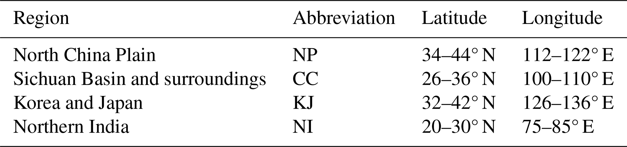
The North China Plain (NP) is one of China's largest plains, characterized by intensive heavy industrial and traffic emissions. The Sichuan Basin and its surrounding areas, encompassing major urban centers such as Chengdu and Chongqing (CC), are defined by an enclosed topographic configuration that severely restricts atmospheric ventilation and promotes pollutant accumulation, thereby producing a topographically driven atmospheric environment fundamentally distinct from that of the other study regions. The Korea and Japan (KJ) region spans the Korean Peninsula and the Japanese archipelago, where NO₂ distributions are significantly influenced by transboundary transport and maritime climatic conditions. Northern India (NI), situated in the Indo-Gangetic Plain, experiences frequent winter haze episodes and agricultural biomass burning. Given the high spatial heterogeneity of NO₂ distributions, the selection of these four representative regions maximizes information density and gradient diversity within the training sample.

2.2 GEMS tropospheric NO₂ data

The Geostationary Environment Monitoring Spectrometer (GEMS), an ultraviolet-visible (UV-Vis) imaging spectrometer onboard the GEO-KOMPSAT-2B (GK-2B) satellite, was launched in February 2020 and became operationally active in November 2022 following in-orbit testing. GEMS provides spectral measurements from 300 to 500 nm with a spectral resolution of approximately 0.6 nm. It achieves a spatial resolution of 3.5 km × 7 km (over Seoul at nadir) and a temporal resolution of one hour. The observational domain of GEMS covers 5° S–45° N and 75–145° E, delivering 6–10 measurements per day over the Asian region (Kim et al., 2020).

This study utilizes the GEMS Level 2 NO₂ tropospheric VCD v3.0 product. To ensure data quality, quality control was applied, retaining only pixels where the VCD is greater than zero, the cloud fraction is less than 0.3, and the solar zenith angle is less than 70°. Thus, negative and zero GEMS retrievals were treated as missing values rather than being replaced with zero. This criterion was adopted because the supervised target was defined as a nonnegative tropospheric NO₂ column field and because the subsequent logarithmic transformation requires nonnegative input values. Pixels removed by this criterion were excluded from the training loss and did not act as zero-valued training labels. The quality-controlled GEMS data were then regridded to a uniform 0.05° × 0.05° latitude-longitude grid using bilinear interpolation to facilitate spatial alignment with other datasets. GEMS data from 1 January to 31 December 2023 were used as the training labels for the model, with data of 2024 reserved for additional validation. Furthermore, all the GEMS data mentioned subsequently refer to the nearest whole-hour time point of their average transit time in that area.

2.3 TROPOMI tropospheric NO₂ data

The TROPOspheric Monitoring Instrument (TROPOMI) is an imaging spectrometer onboard the European Space Agency's (ESA) Sentinel-5 Precursor (S5P) satellite, which was launched on 13 October 2017 (Veefkind et al., 2012; Ialongo et al., 2020). S5P operates in a sun-synchronous polar orbit at an altitude of approximately 824 km, achieving daily global coverage with an equator crossing time of around 13:30 local time (LT). TROPOMI employs a push-broom imaging technique with a wide swath of 2600 km. Its spectral range covers the ultraviolet, visible, near-infrared, and shortwave infrared bands (270–2385 nm), with the NO₂ retrieval primarily relying on the visible band (405–465 nm) (van Geffen et al., 2025) and the cloud retrieval relying on UV/visible/NIR bands (Loyola et al., 2018). The instrument's spatial resolution was enhanced from 7 × 3.5 to 5.5 × 3.5 km² (across-track × along-track) on 6 August 2019 (Liu et al., 2021a), making it the highest-resolution operational sensor for NO₂ monitoring on a polar-orbiting platform.

The TROPOMI NO₂ product has been validated against ground-based Pandora spectrometers, Multi-Axis Differential Optical Absorption Spectroscopy (MAX-DOAS) observations, and aircraft campaigns, demonstrating high accuracy (Griffin et al., 2019; Ialongo et al., 2020; Verhoelst et al., 2021). This study uses the TROPOMI Level 2 tropospheric NO₂ VCD products from 2019 to 2024, with data from 2023 employed for model training. For TROPOMI data, a quality assurance flag (qa_value) greater than 0.75 was used as the filtering criterion. The filtered data were subsequently regridded to the same 0.05° × 0.05° grid using the HARP toolkit (https://github.com/stcorp/harp, last access: 9 June 2026). In addition to the qa_value threshold, TROPOMI retrievals with tropospheric NO₂ VCD values less than or equal to zero were treated as missing. This filtering maintained consistency with the nonnegative model-input domain and the logarithmic normalization used in the framework.

2.4 GOME-2 tropospheric NO₂ data

GOME-2 (Global Ozone Monitoring Experiment-2) is an ultraviolet-visible imaging spectrometer onboard the MetOp series of satellites operated by the European Organisation for the Exploitation of Meteorological Satellites (EUMETSAT). The GOME-2 series consists of three satellites: MetOp-A (launched in October 2006), MetOp-B (launched in September 2012), and MetOp-C (launched in November 2018). GOME-2 has a local overpass time of approximately 09:30 and provides daily global coverage (Munro et al., 2016).

The GOME-2 NO₂ products (Valks et al., 2011) have undergone long-term validation and improvement. Comparison studies with ground-based MAX-DOAS, Pandora observations, and other satellite products have demonstrated good consistency at both global and regional scales (Pinardi et al., 2010; Liu et al., 2019). This study utilizes the GOME-2C Level 2 daily tropospheric NO₂ product provided by EUMETSAT AC-SAF (Hassinen et al., 2016). The nominal native ground-pixel size of GOME-2C is 80 km × 40 km for forward-scan observations and 240 km × 40 km for back-scan observations (Chan et al., 2023). The data were regridded to a 0.25° × 0.25° resolution using the HARP toolkit, and pixels with a cloud fraction greater than 0.3 were filtered out. For consistency with the GEMS and TROPOMI processing, GOME-2 retrievals with tropospheric NO₂ VCD values less than or equal to zero were also excluded. This product is primarily used for the cross-comparison and independent validation of the model's prediction results in subsequent chapters. Given the significant difference between GOME-2's overpass time and those of TROPOMI and GEMS, its data offer an independent reference for assessing the diurnal variation of NO₂ and the model's temporal generalization capability.

2.5 Pandora ground-based NO₂ observations

Pandora is a ground-based ultraviolet–visible spectrometer system that measures atmospheric trace gases, including NO₂, using direct-sun and scattered-sky observations (Herman et al., 2009). The Pandonia Global Network (PGN) coordinates the processing and distribution of Pandora measurements to support air-quality monitoring and satellite validation (Verhoelst et al., 2021; Park et al., 2026). Its high temporal resolution provides a ground-based reference for evaluating the temporal variability of satellite observations and reconstructed products. This study uses the rnvh3p1-8 tropospheric NO₂ column product derived from sky-scanning observations. Observations available during 2019–2024 were obtained as an external reference independent of model training. Usable observations were identified at 16 stations: Beijing-RADI in NP; Busan, Daegu, Fukuoka, Incheon-ESC, Jeonju, Kobe, Seosan, Seoul, Seoul-KU, Seoul-SNU, Suwon-USW, Ulsan, and Yongin in KJ; Haldwani-ARIES and Nainital-ARIES in NI. No eligible station was identified in CC for this evaluation. Observational coverage varied among stations and years.

The evaluation used finite positive tropospheric NO₂ columns with quality flags 10 or 11, corresponding to preliminary high- and medium-quality estimates, respectively, that had not undergone formal quality assurance. Low-quality observations (flag 12) were excluded, and no additional upper concentration threshold was applied. Column amounts were converted from mol m⁻² to Pmolec. cm⁻². At Seoul-SNU, Pandora 149 was used preferentially, and Pandora 163 supplied only hours without valid observations from Pandora 149, avoiding duplicate station-hour samples. The rnvh3 tropospheric column represents approximately the surface-to-4 km column; differences in vertical sensitivity and spatial sampling relative to satellite retrievals should therefore be considered when interpreting the comparisons.

2.6 ERA5 meteorological reanalysis data

Meteorological conditions play a decisive role in influencing the spatiotemporal heterogeneity of tropospheric NO₂ through physical transport and chemical modulation processes. This study uses the fifth generation of the European Centre for Medium-Range Weather Forecasts (ECMWF) atmospheric reanalysis, ERA5 (Hersbach et al., 2020). This dataset is produced using the Integrated Forecasting System (IFS) Cycle 41r2, which assimilates a vast range of global observations through a 4D-Var data assimilation system. It provides data at a spatial resolution of 0.25° × 0.25° and an hourly temporal resolution. ERA5 has been widely adopted in atmospheric chemistry research, serving as a meteorological driver for chemical transport models (CTMs), as auxiliary input for satellite retrievals, and as feature variables in machine learning models (Zhang et al., 2025b; Mols et al., 2026).

Both single-level and pressure-level variables from ERA5 were utilized in this study. The single-level variables include boundary layer height (blh), surface pressure (sp), and total cloud cover (tcc). Boundary layer height is a key physical parameter governing near-surface NO₂ concentrations (Huang et al., 2021; von Engeln and Teixeira, 2013) and indirectly influences satellite-retrieved tropospheric NO₂ VCDs through the lower-tropospheric contribution to the column. Surface pressure not only indicates the evolution of weather systems but also directly affects the normalization of a priori profiles and the weighting of lower-layer contributions in the calculation of air mass factor (AMF) (Boersma et al., 2007). Total cloud cover modulates the photolysis rate of NO₂ and photochemical equilibrium by altering shortwave radiation reaching the lower atmosphere (van Weele and Duynkerke, 1993), while also being closely linked to precipitation and local thermal circulations (Sfica et al., 2021). For multi-level variables, specific humidity (q), temperature (T), and horizontal wind components (u,v) were extracted at four levels: 500, 850, 925, and 1000 hPa. Lower-level variables can capture thermodynamic and dynamic conditions near NO₂ emission sources, whereas the 500 hPa level represents the large-scale circulation background and vertical transport potential in the mid-troposphere (Wang et al., 2026). Temperature and specific humidity jointly determine the thermodynamic conditions and oxidant environment for atmospheric chemical reactions (Mentel et al., 1996; Wang et al., 2020). The wind components provide vector information on the horizontal transport of pollutants. All ERA5 variables used are hourly data at a 0.25° resolution, serving as part of the low-resolution channels input to the model.

2.7 EAC4 reanalysis data

The ECMWF Atmospheric Composition Reanalysis 4 (EAC4) is a core data product of the Copernicus Atmosphere Monitoring Service (CAMS), providing a spatiotemporally consistent reanalysis of global atmospheric composition from 2003 to the present (Inness et al., 2019). EAC4 is based on the atmospheric chemistry module of the ECMWF's IFS and assimilates multi-source satellite observations with model forecasts using a 4D-Var scheme to produce chemically consistent and spatiotemporally complete atmospheric composition fields (Flemming et al., 2015).

This study employs the total column NO₂ (tcno2) variable from EAC4 as an input feature. Because tcno2 includes both tropospheric and stratospheric NO₂, it is not directly equivalent to the GEMS tropospheric VCD used as the supervised target. EAC4 is therefore used as a spatially complete, coarse-resolution chemical background prior rather than a target-equivalent representation of tropospheric NO₂. Although it differs from the satellite-observed tropospheric NO₂ concentration, this product provides a spatiotemporally complete a priori estimate of the NO₂ field, thereby enriching valuable physical prior information available to the model. The original EAC4 product has a temporal resolution of 3 h and a spatial resolution of 0.75° × 0.75°. To align with the overall framework, EAC4 data were resampled to a 1 h temporal resolution and a 0.25° × 0.25° spatial resolution using linear interpolation, making it consistent with the ERA5 reanalysis data.

2.8 MCD12C1 land cover data

Land use/land cover (LULC) type is a critical factor influencing the spatial distribution of NO₂. Different land use types correspond to distinct emission source characteristics and intensities: urban and built-up areas concentrate emissions from traffic, industry, and residential activities; agricultural lands are associated with emissions from farm machinery and soil nitrogen cycles; and forests and grasslands are primarily influenced by natural emissions and biomass burning (Lamsal et al., 2013; Song et al., 2019). Furthermore, land use types indirectly affect the accuracy of satellite retrievals and local meteorological conditions by influencing surface albedo and roughness (Auer, 1978; Noguchi et al., 2014). Consequently, incorporating land use information as a spatial prior helps the model to better understand the heterogeneity of NO₂ spatial patterns.

This study uses the annual MODIS Version 6.1 Climate Modeling Grid (CMG) land cover product, MCD12C1, for the years 2019–2023 (Friedl and Sulla-Menashe, 2022). The Leaf Area Index (LAI)-based classification scheme (LCType3) was selected. Given the mismatch in spatial resolution between MCD12C1 (0.05°) and physical driver fields (0.25°), the land cover data were spatially aggregated to the 0.25° grid by averaging.

2.9 ETOPO 2022 elevation data

Topography is another essential spatial prior variable. Elevation is directly related to atmospheric pressure and air density (Zhou et al., 2009), while topographical variations influence local circulation patterns (e.g., valley and slope winds) and pollutant transport pathways (Gohm et al., 2009). Topography is also closely linked to the spatial distribution of emission sources, as human activities and NO₂ emissions are predominantly concentrated in low-lying plains and basins, whereas emissions are sparse in high-altitude mountains and plateaus (Lamsal et al., 2013; Yuan et al., 2025). Additionally, terrain elevation affects the calculation of the AMF in satellite retrievals, with higher uncertainty typically observed over high-altitude areas (Boersma et al., 2011). Therefore, integrating topographical information into the model enhances its predictive capability for NO₂ distribution, especially in regions with complex terrain.

This study utilizes the Earth TOPOgraphy (ETOPO) 2022 global relief model (NOAA National Centers for Environmental Information, 2022). As the latest version in the ETOPO series, it integrates multi-source topographic and bathymetric data, including satellite altimetry, shipborne sonar, airborne gravity, and terrestrial digital elevation models, to provide a high-resolution global relief dataset for land and ocean (MacFerrin et al., 2025). This study utilizes the 60 arcsec resolution version, which was resampled to a 0.25° × 0.25° resolution via spatial aggregation (averaging) to align with the grid of the other physical variables.

3 Methodology

3.1 Multi-source data integration framework

This study integrates multi-source datasets with heterogeneous origins, spatiotemporal resolutions, and physical units, constructing an input tensor system comprising two 0.05° high-resolution input channels (the TROPOMI tropospheric NO₂ VCD and its validity mask), 33 low-resolution predictor channels at 0.25° resolution, and one supervised target channel consisting of the quality-controlled 0.05° hourly GEMS tropospheric NO₂ VCD. Table 2 systematically summarizes the source, original resolution, physical significance, and normalization strategy of all input variables. All reconstructed hourly fields correspond to daytime GEMS observation hours.

Table 2 Summary of input variables for PhysNorm-Net.

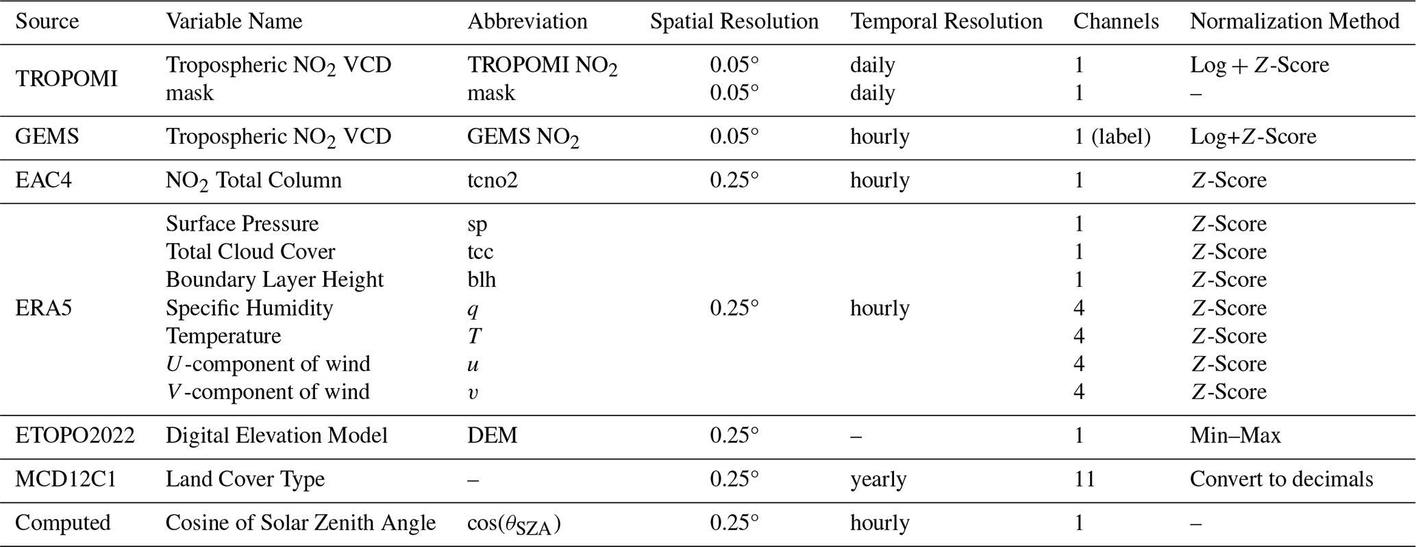
Note: The 4 channels for ERA5 multi-level variables correspond to 1000, 925, 850, and 500 hPa pressure levels. The 11 channels for MCD12C1 represent the 11 land cover types.

To ensure numerical stability during neural network training and eliminate the influence of dimensional discrepancies on gradient propagation, differentiated normalization strategies were tailored to the characteristics of each variable type. Prior to normalization, the 2023 dataset was randomly partitioned by date into training (256 d), validation (54 d), and test (55 d) sets. This split was used for model development and for evaluating performance on held-out dates within 2023. Because randomly selected dates may have weather conditions similar to those of nearby training dates, the 2023 test set is not interpreted as a strictly temporally independent evaluation. The complete 2024 dataset was retained outside the 2023 data split and used for independent-year validation.

The probability distribution of tropospheric NO₂ column densities exhibits a pronounced positive skew, with several orders of magnitude separating high-value tails (corresponding to pollution events) from background concentrations. A direct linear scaling would compress the information content of high-concentration pixels while disproportionately amplifying minor variations in low-concentration regions, thereby hindering the model's ability to learn the spatial features of both pollution hotspots and background areas. To address this, TROPOMI and GEMS tropospheric NO₂ VCDs were first scaled by a factor of 10⁻¹⁵ (converting to units of Pmolec. cm⁻²), followed by logarithmic transformation and Z-score normalization:

$$\begin{array}{}\text{(1)}& {\displaystyle }{x}_{\log }=\ln \left(x_{\mathrm{trop}}+\mathit{ϵ}\right)\text{(2)}& {\displaystyle }{x}_{\mathrm{norm}}={\displaystyle \frac{x_{\log }-{\mathit{\mu }}_{\log }}{{\mathit{\sigma }}_{\log }}}\end{array}$$

Here, ϵ is a small constant to prevent undefined logarithms for zero values, while μ_log and σ_log represent the global mean and standard deviation of the log-transformed training data, respectively. The logarithm transform effectively compresses the dynamic range of the data, making its distribution more Gaussian-like while preserving the relative relationships between concentration gradients. The subsequent Z-score standardization centers the data and scales it to a standard deviation of one, aligning it with the standard input assumptions of deep neural networks (LeCun et al., 2012).

For ERA5 and EAC4 reanalysis variables, Z-score normalization was uniformly applied:

$$\begin{array}{}\text{(3)}& x{}^{\prime }={\displaystyle \frac{x-\mathit{\mu }}{\mathit{\sigma }}}\end{array}$$

where μ and σ are the spatiotemporal statistics of each variable computed over the training set. It is emphasized that all normalization statistics are derived exclusively from the training set and subsequently applied to the validation and test sets to strictly prevent data leakage.

Since DEM data possess well-defined physical boundaries (from sea level to the highest peak) and their absolute values carry physical meaning, a min-max normalization was applied to preserve this characteristic while mapping values to the [0, 1] interval:

$$\begin{array}{}\text{(4)}& z{}^{\prime }={\displaystyle \frac{z-z_{\min }}{z_{\max }-z_{\min }}}\end{array}$$

where z_max and z_min are the global maximum and minimum DEM values.

Land use data from MCD12C1 are provided as area fractions (original values as percentages from 0–100); these were directly converted to decimals in the [0, 1] range by dividing by 100. Normalization of both DEM and land use data was performed prior to spatial resampling.

For temporal encoding, while spatiotemporal prediction tasks typically employ periodic functions (e.g., sine/cosine transforms) to explicitly embed hour, day, or year cycles, such purely mathematical encodings may lack a direct connection to atmospheric physical processes. Therefore, this study proposes using the cosine of the solar zenith angle (cos(θ_SZA)) as a substitute for conventional time encoding. For a given UTC time, regions at different longitudes experience different local solar times and corresponding SZAs. The SZA implicitly encodes the longitude-time coupling, enabling the model to understand local illumination conditions without needing to learn complex time zone conversion logic. Furthermore, the SZA reflects both diurnal and seasonal variations (depending on solar declination), allowing a single variable to represent periodicity across multiple time scales and reducing input feature redundancy.

The calculation process is as follows: based on the UTC timestamp and the central coordinates of the region, the solar elevation angle (α) is first computed using a solar position algorithm (Reda and Andreas, 2004), from which the solar zenith angle (θ_SZA) is derived:

$$\begin{array}{}\text{(5)}& {\mathit{\theta }}_{\mathrm{SZA}}=\mathrm{90}\mathit{°}-\mathit{\alpha }\end{array}$$

To constrain input values within the numerical range preferred by neural networks, the cosine is taken:

$$\begin{array}{}\text{(6)}& f_{\mathrm{SZA}}=\cos \left({\mathit{\theta }}_{\mathrm{SZA}}\right)\end{array}$$

This value approaches 0 near sunrise/sunset and approaches 1 at solar noon in tropical regions (or less than 1 at mid-to-high latitudes), offering intuitive physical interpretation. Given that the spatial resolution of data such as EAC4 is 0.25°, corresponding to a grid scale of approximately 25–30 km, the spatial variation of the SZA within this scale is negligible (< 0.1°). Therefore, f_SZA is treated as a spatially uniform field and appended to the low-resolution tensor.

3.2 Overall architecture of PhysNorm-Net

Let the high-resolution TROPOMI NO₂ observations be denoted as $X_{\mathrm{obs}}\in {\mathbb{R}}^{H\times W}$. Due to cloud cover, aerosol contamination, and sensor swath gaps, the observation field is spatially sparse. Therefore, a binary mask $M\in {\left\{\mathrm{0},\mathrm{1}\right\}}^{H\times W}$ is introduced to mark the locations of valid pixels (1 for valid, 0 for missing). Concurrently, to incorporate the dynamic constraints of atmospheric transport and dispersion, a set of spatiotemporally aligned, low-resolution physical and topography data is utilized, denoted as $P\in {\mathbb{R}}^{h\times w\times C}$, where h<H, w<W, and C is the number of physical variable channels. The objective of this study is to learn a nonlinear mapping function ℱ that infers the complete, high-spatiotemporal-resolution NO₂ field $\widehat{Y}$ by fusing the sparse observations with the dense physical prior:

$$\begin{array}{}\text{(7)}& \widehat{Y}=\mathcal{F}\left({\mathrm{X}}_{\mathrm{obs}},P,M\right)\end{array}$$

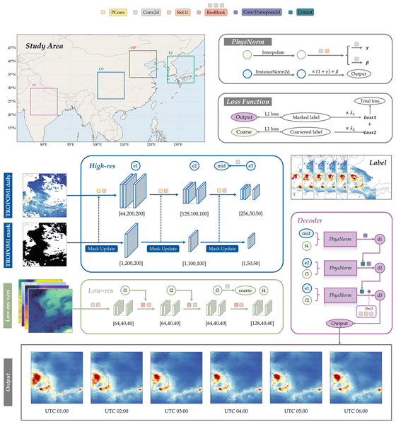
The challenge inherent in this problem lies in the significant modality gap between X_obs and P: the former contains high-frequency spatial textures but is incomplete, while the latter is physically continuous but spatially coarse. To address this multi-modal fusion challenge, the PhysNorm-Net is designed. As illustrated in Fig. 1, the network's main body inherits the classic U-Net architecture (Ronneberger et al., 2015), comprising a contracting path (encoder) and an expansive path (decoder), with skip connections to preserve multi-scale features. However, two critical asymmetric modifications are introduced to the standard U-Net to accommodate irregularly missing data and to integrate physical constraints:

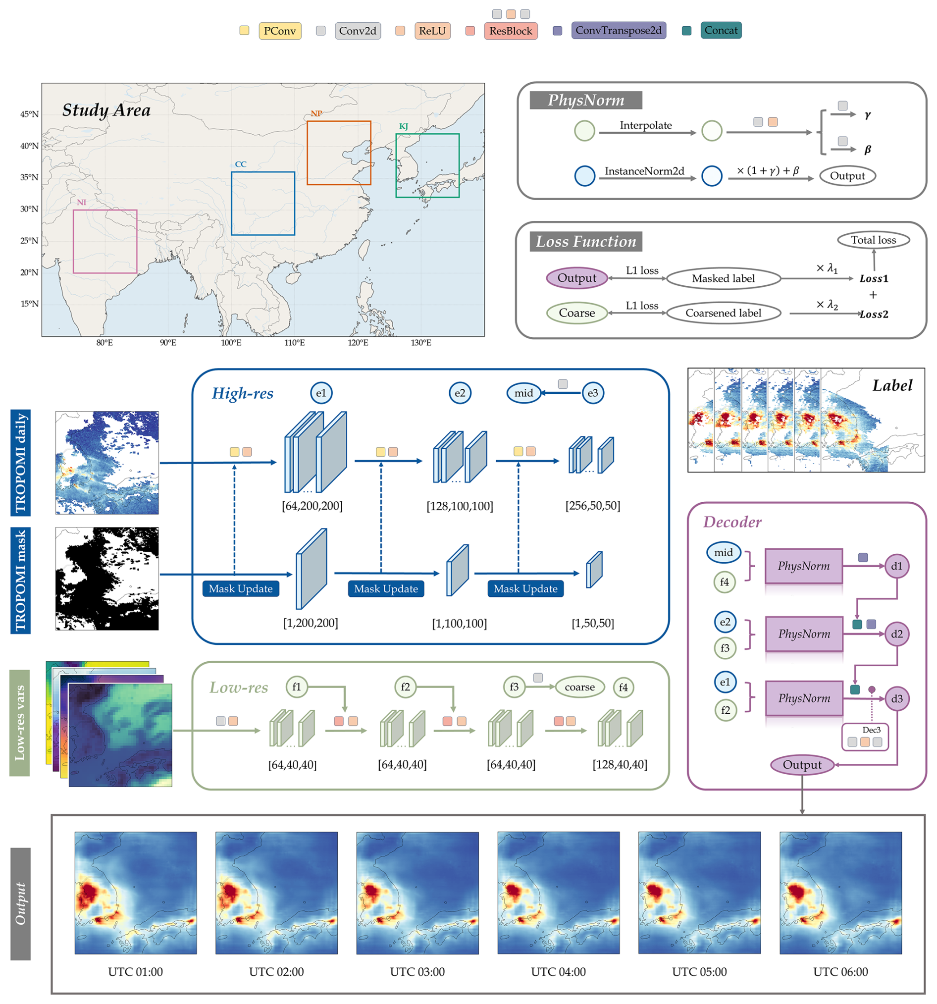
Figure 1 Architecture diagram of PhysNorm-Net.

The Main Observation Stream, which forms the U-Net backbone, is responsible for extracting multi-scale features from the spatially incomplete TROPOMI field. Unlike traditional Convolutional Neural Networks (CNNs) that use standard convolutional layers, this stream is constructed from a stack of Partial Convolution layers. This enables the network to adaptively handle data missing in arbitrary shapes, progressively in-painting the feature maps during the encoding process.

The Physics-Conditional Stream operates as a parallel feature extractor, deriving latent physical information from the low-resolution data. This stream employs a deep residual network (ResNet) structure to prevent gradient vanishing during deep feature extraction and to ensure the effective propagation of physical information.

During the decoding (upsampling) phase, features from the physics stream are not simply concatenated with the observation features. Instead, they are used to dynamically modulate the statistical distribution of the observation features through a novel Physics-Aware Normalization (PhysNorm) module. This conditional affine transformation fuses the two streams of information to reconstruct the high-resolution tropospheric NO₂ field. This design ensures that the generated pollutant concentration field not only retains the fine details from the satellite observations but also adheres macroscopically to the prevailing meteorological dispersion patterns.

3.3 Observation encoding via Partial Convolution

Spatial gaps in satellite remote sensing imagery exhibit high irregularity, with patterns, areas, and locations varying across samples. Standard convolution operations implicitly assume all input pixels are valid and incorporate padded values (e.g., zeros or mean-filled values) in missing regions into feature calculations. This leads to the contamination of features from valid areas by missing areas, an error that propagates and diffuses throughout the feature map as network depth increases. To resolve this issue, this study adopts the Partial Convolution (PConv) layer, proposed by Liu et al. (2018), as the fundamental operator in the encoder. The core mechanism of PConv is to perform convolution exclusively on the valid pixels defined by a mask and to re-weight the result based on the proportion of valid pixels.

Assume the input feature at layer l is X^(l), the corresponding binary mask is M^(l), the convolution kernel is W, and the bias is b. The partial convolution output at position (i,j) is computed as:

$$\begin{array}{}\text{(8)}& \begin{array}{rl}& x_{\left(i,j\right)}{}^{\prime }=\\ & \left\{\begin{array}{ll}& W^T{\left(X^{\left(l\right)}\odot M^{\left(l\right)}\right)}_{\left(i,j\right)}\cdot \frac{\mathrm{sum}\left(\mathrm{1}\right)}{\mathrm{sum}{\left(M^{\left(l\right)}\right)}_{\left(i,j\right)}}+b,\mathrm{if}\mathrm{sum}{\left(M^{\left(l\right)}\right)}_{\left(i,j\right)}>\mathrm{0}\\ & \mathrm{0},\mathrm{otherwise}\end{array}\right.\end{array}\end{array}$$

Here, ⊙ denotes element-wise multiplication, sum(1) is the total number of pixels in the convolutional window, and $\mathrm{sum}{\left(M^{\left(l\right)}\right)}_{\left(i,j\right)}$ is the number of valid pixels within that window. The scaling factor $\frac{\mathrm{sum}\left(\mathrm{1}\right)}{\mathrm{sum}{\left(M^{\left(l\right)}\right)}_{\left(i,j\right)}}$ automatically corrects for the reduction in signal strength caused by the diminished amount of valid information. Simultaneously, the mask is updated after each layer: a position in the next layer's mask is marked as valid if at least one valid pixel existed within its receptive field in the current layer. This hierarchical update mechanism enables valid information to propagate layer-by-layer toward missing regions as network depth increases, providing the decoder with structurally complete semantic features.

Specifically, the high-resolution encoder employs a three-stage downsampling architecture. The first stage uses a 7 × 7 large-kernel convolution (64 channels) to rapidly expand the receptive field while preserving the original resolution, which is suitable for capturing medium-scale NO₂ spatial structures. The subsequent two stages use 3 × 3 convolutions (128 and 256 channels, respectively) to perform 2× downsampling. The feature maps and updated masks at each stage are preserved for use in the decoder via skip connections.

3.4 Residual encoding of physical priors

The physical prior encoding module is tasked with extracting a hierarchical feature representation of the atmospheric state from the low-resolution tensor $P\in {\mathbb{R}}^{h\times w\times C}$. The design objectives for this module are: (a) to capture the nonlinear mapping relationships between meteorological fields, surface characteristics, and NO₂ distribution; and (b) to generate multi-level physical features for fusion at different resolution scales in the decoder. Traditional deep convolutional networks, after alternating between multiple layers of linear convolution and nonlinear activation, are prone to gradient degradation, which can lead to the over-abstraction or even loss of spatially continuous information present in the original meteorological data. Therefore, this module adopts a residual network (ResNet) architecture, consisting of an initial convolutional layer followed by three residual blocks. The introduction of residual connections alleviates gradient vanishing in deep networks (He et al., 2015) while facilitating the learning of incremental functions near identity mappings from input to output. This network produces three levels of physical feature maps $\left\{F_{\mathrm{phy}}^{\left(\mathrm{1}\right)},F_{\mathrm{phy}}^{\left(\mathrm{2}\right)},F_{\mathrm{phy}}^{\left(\mathrm{3}\right)}\right\}$ (with 64, 64, and 128 channels, corresponding to f2, f3, f4 in Fig. 1), which encode hierarchical information from raw meteorological variables to abstract physical patterns.

Specifically, the low-resolution input is first mapped to a latent feature space via an initial convolutional layer, followed by deep feature extraction through a stack of residual blocks. If the input feature to the kth residual block is $F_{\mathrm{phy}}^{(k-\mathrm{1})}$, the feature propagation process can be described as:

$$\begin{array}{}\text{(9)}& F_{\mathrm{phy}}^{\left(k\right)}=\mathrm{ReLU}\left(F_{\mathrm{phy}}^{\left(k-\mathrm{1}\right)}+{\mathcal{R}}_k\left(F_{\mathrm{phy}}^{\left(k-\mathrm{1}\right)}\right)\right)\end{array}$$

where ℛ_k represents the residual mapping composed of two consecutive convolutional layers with embedded nonlinear activation functions. The identity mapping term $F_{\mathrm{phy}}^{(k-\mathrm{1})}$ allows fundamental physical information provided by the low-resolution branch to be directly transmitted to deeper network layers. The residual term ℛ_k(⋅) is consequently forced to learn only refinements (or perturbations). The physical prior encoder does not merely output a single global feature vector but extracts multi-scale hierarchical features under different receptive fields. These features are then routed to and precisely aligned with the PhysNorm modules at different depths of the high-resolution decoder.

Additionally, this module includes an auxiliary prediction head (a 1 × 1 convolution layer) that directly predicts a coarse-resolution NO₂ field ${\widehat{Y}}_{\mathrm{coarse}}$ from the intermediate feature layer $F_{\mathrm{phys}}^{\left(\mathrm{2}\right)}$. This auxiliary output provides an additional supervisory signal during training (detailed in Sect. 3.6), ensuring that the physical features possess direct predictive capability for NO₂ concentrations.

3.5 Physics-Aware Normalization (PhysNorm) module and multi-scale decoder

A core challenge of this research is how to effectively fuse low-resolution physical information during the decoder's process of recovering high-resolution details. Traditional fusion methods, such as concatenation or addition, treat physical information as an additional feature channel, relying on the network to implicitly learn its relationship with satellite observations. This often leads to the deep learning network prioritizing the observational data and ignoring the physics stream, causing the model to degrade into image interpolation. Inspired by Spatially-Adaptive (De)normalization (SPADE) from the image generation domain (Park et al., 2019), this study proposes the Physics-Aware Normalization module. This module treats the meteorological field as an environmental context that dynamically modulates the normalized statistics of the satellite feature map via an affine transformation. The workflow of PhysNorm involves three main steps:

Destylization: First, the input satellite feature map (F_sat, corresponding to mid, e2, e1 in Fig. 1) undergoes parameter-free Instance Normalization (IN). This step removes biases in absolute concentration that are specific to a particular time and region by subtracting the mean and dividing by the standard deviation, thereby retaining the pure relative structural information:

$$\begin{array}{}\text{(10)}& {\widehat{F}}_{\mathrm{sat}}={\displaystyle \frac{F_{\mathrm{sat}}-\mathit{\mu }\left(F_{\mathrm{sat}}\right)}{\mathit{\sigma }\left(F_{\mathrm{sat}}\right)}}\end{array}$$

Parameter Mapping: Using the multi-scale features (F_phy) extracted by the physics encoder, two separate shallow convolutional networks, ϕ_γ and ϕ_β, learn the scaling (γ) and shifting (β) coefficients corresponding to the specific meteorological conditions:

$$\begin{array}{}\text{(11)}& \mathit{\gamma }={\mathit{\varphi }}_{\mathit{\gamma }}\left(F_{\mathrm{phy}}\right),\mathit{\beta }={\mathit{\varphi }}_{\mathit{\beta }}\left(F_{\mathrm{phy}}\right)\end{array}$$

Here, γ and β are tensors of the same spatial dimensions as ${\widehat{F}}_{\mathrm{sat}}$.

Physics Injection: The learned parameters are then used to modulate the normalized features:

$$\begin{array}{}\text{(12)}& F_{\mathrm{out}}={\widehat{F}}_{\mathrm{sat}}\cdot \left(\mathrm{1}+\mathit{\gamma }\right)+\mathit{\beta }\end{array}$$

The scaling factor γ and shifting factor β control the local concentration contrast and background level, respectively. For instance, under conditions of strong winds and high dispersion, where the pollutant distribution tends to be more uniform, the model would predict smaller γ values to suppress local peaks. In areas with a low boundary layer height or high emissions, the model would generate positive β values to holistically elevate the predicted concentrations in that region. Through PhysNorm, the model can be compelled to rely on the physical state (low-resolution input) to determine the numerical range and distribution intensity of the final output, fundamentally resolving the information imbalance issue in modality fusion.

The decoder adopts a symmetric three-stage upsampling architecture, progressively recovering spatial resolution via transposed convolutions. PhysNorm is deployed at each decoder stage, modulated by the deep, intermediate, and shallow features from the physical prior module, respectively. This hierarchical design allows physical information of varying abstraction levels to act on corresponding spatial scales: deep features modulate weather-scale patterns, while shallow features modulate variations at the local scale.

In this architecture, the PhysNorm module modulates encoder features prior to concatenation. The final output layer is a lightweight convolutional head (two 3 × 3 convolutional layers, 128 → 32 → 1 channels), which maps the fused features to a single-channel NO₂ prediction field.

3.6 Dual-task loss function

To maintain physical consistency while ensuring high-resolution reconstruction accuracy, this study proposes a dual-task constrained loss function. The total loss is a linear combination of a fine-grained reconstruction loss and a coarse-grained physical consistency loss:

$$\begin{array}{}\text{(13)}& {\mathcal{L}}_{\mathrm{total}}={\mathit{\lambda }}_{\mathrm{1}}{\mathcal{L}}_{\mathrm{fine}}+{\mathit{\lambda }}_{\mathrm{2}}{\mathcal{L}}_{\mathrm{coarse}}\end{array}$$

The fine-grained reconstruction loss (ℒ_fine) supervises the final high-resolution output of the U-Net. Since the ground truth labels (GEMS data) themselves contain missing values, the loss is computed only over valid pixels. An L1 loss is adopted to enhance robustness against outliers in satellite data.

The physical consistency loss (ℒ_coarse) supervises the coarse-resolution prediction from the physical prior module. The GEMS labels are downsampled to the low-resolution grid after handling invalid values, and the loss is computed in the same masked L1 form. This auxiliary task ensures that the physical features possess direct predictive capability for NO₂ and provides a more direct gradient signal to the shallow layers of the network, alleviating the gradient dilution problem in deep networks. In our setup, both λ₁ and λ₂ are set to 1.0.

3.7 Evaluation metrics

This study employs multiple evaluation metrics to assess model performance, all of which are calculated based on valid observation pixels. Detailed descriptions follow:

The coefficient of determination (R²) measures the extent of the variance between predictions and original observations. It is defined as:

$$\begin{array}{}\text{(14)}& R^{\mathrm{2}}=\mathrm{1}-{\displaystyle \frac{{\sum }_{i=\mathrm{1}}^n(y_i-{\widehat{y}}_i{)}^{\mathrm{2}}}{{\sum }_{i=\mathrm{1}}^n(y_i-\stackrel{\mathrm{‾}}{y}{)}^{\mathrm{2}}}}\end{array}$$

where y_i and ${\widehat{y}}_i$ are the observed and predicted values for the ith sample, $\stackrel{\mathrm{‾}}{y}$ is the mean of the observed values, and n is the total number of samples. R² ranges from −∞ to 1, with values closer to 1 indicating a better fit. To evaluate the statistical significance of R², the F-test is employed to compute its associated probability (p-value). The F-statistic is defined as:

$$\begin{array}{}\text{(15)}& F={\displaystyle \frac{R^{\mathrm{2}}/k}{\left(\mathrm{1}-R^{\mathrm{2}})/(n-k-\mathrm{1}\right)}}\end{array}$$

where k is the number of independent variables in the regression model. Under the null hypothesis ($R_{\mathrm{true}}^{\mathrm{2}}=\mathrm{0}$), F follows an F-distribution with degrees of freedom $(k,n-k-\mathrm{1})$. The p-value is computed via the survival function of the F-distribution, and p< 0.05 indicates that R² is significantly different from zero at the 95 % confidence level.

When validating against another independent source (e.g., the LEO satellite GOME-2), which may have inherent differences in retrieval algorithms and observation geometries, this study uses the Pearson correlation coefficient (R) as the core metric for cross-validation:

$$\begin{array}{}\text{(16)}& R={\displaystyle \frac{{\sum }_{i=\mathrm{1}}^n\left(y_i-\stackrel{\mathrm{‾}}{y}\right)\left({\widehat{y}}_i-\stackrel{\mathrm{‾}}{\widehat{y}}\right)}{\sqrt{{\sum }_{i=\mathrm{1}}^n{\left(y_i-\stackrel{\mathrm{‾}}{y}\right)}^{\mathrm{2}}}\sqrt{{\sum }_{i=\mathrm{1}}^n{\left({\widehat{y}}_i-\stackrel{\mathrm{‾}}{\widehat{y}}\right)}^{\mathrm{2}}}}}\end{array}$$

where $\stackrel{\mathrm{‾}}{\widehat{y}}$ is the mean of predicted values. Pearson R ranges from −1 to 1, and values closer to ±1 indicate stronger linear correlation.

Root Mean Square Error (RMSE) quantifies the overall magnitude of the prediction error. It is defined as:

$$\begin{array}{}\text{(17)}& \mathrm{RMSE}=\sqrt{{\displaystyle \frac{\mathrm{1}}{n}}{\sum }_{i=\mathrm{1}}^n(y_i-{\widehat{y}}_i{)}^{\mathrm{2}}}\end{array}$$

RMSE has the same units as the observations (Pmolec. cm⁻²), facilitating a direct assessment of the error's actual magnitude.

Mean Absolute Error (MAE) measures the average magnitude of the errors, assigning equal weight to each error. It is defined as:

$$\begin{array}{}\text{(18)}& \mathrm{MAE}={\displaystyle \frac{\mathrm{1}}{n}}{\sum }_{i=\mathrm{1}}^n\mid y_i-{\widehat{y}}_i\mid \end{array}$$

Compared to RMSE, MAE is more robust to outliers. Using both metrics can reveal characteristics of the error distribution: an RMSE value significantly larger than the MAE suggests the presence of a few samples with large errors.

Normalized Mean Bias (NMB) normalizes the mean bias relative to the mean of the observations, enabling comparable assessments across different regions and time periods. It is defined as:

$$\begin{array}{}\text{(19)}& \mathrm{NMB}={\displaystyle \frac{{\sum }_{i=\mathrm{1}}^n({\widehat{y}}_i-y_i)}{{\sum }_{i=\mathrm{1}}^n{y}_i}}\end{array}$$

NMB expresses the relative degree of systematic bias as a percentage, eliminating the influence of varying absolute NO₂ concentrations across different regions or seasons.

4 Results

4.1 Overall dataset accuracy and spatiotemporal consistency

To characterize model performance on held-out dates within the 2023 training year, Fig. 2 presents the overall scatter density plots for the training, validation, and test sets. The predicted dataset achieved high prediction accuracy across all three sets, with R² values of 0.939, 0.882, and 0.889, respectively (all p-values < 0.01). Furthermore, during the training and testing process involving tens of millions of samples, the performance metrics on the validation and test sets were highly consistent, with no significant signs of overfitting. This indicates that the designed PhysNorm-Net model can effectively learn the non-linear mapping relationship between multi-source physical drivers and pollutant concentrations. Although this evaluation directly examines model performance under naturally occurring TROPOMI gaps wherever valid GEMS references are available, reconstructed pixels for which GEMS itself is unavailable cannot be directly verified against GEMS. Therefore, the reported metrics should not be interpreted as a pixelwise validation of the entire gapless product.

Figure 2 Scatter density plots of model predictions versus original GEMS observations.

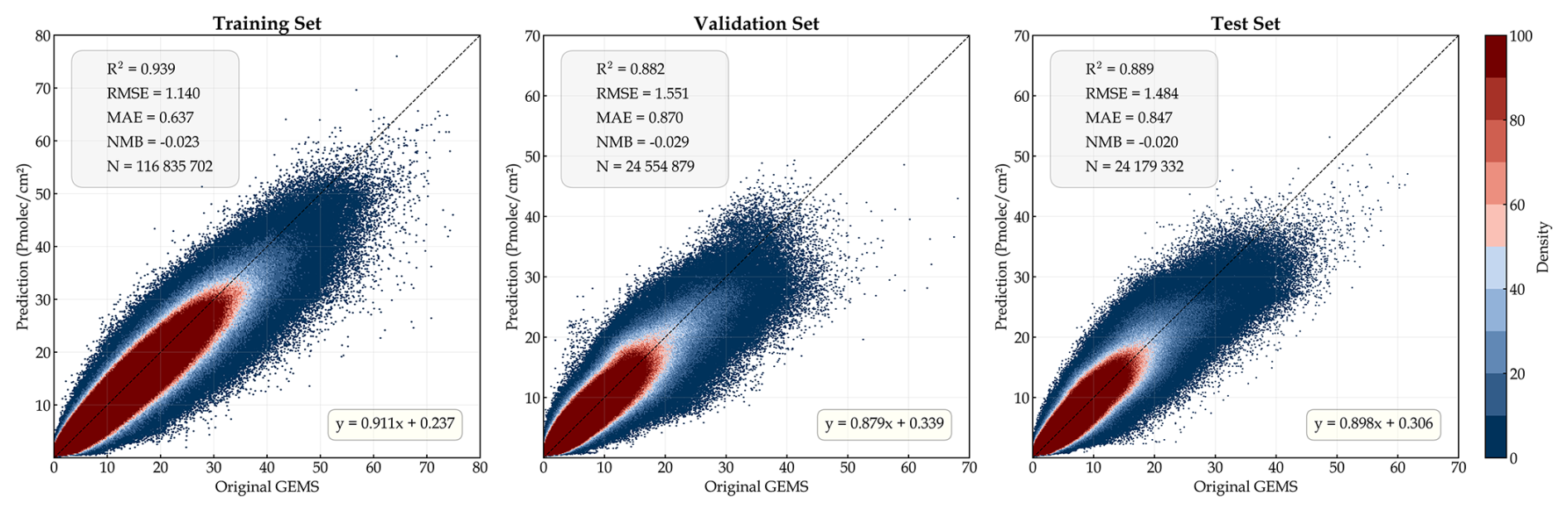
Notably, the predicted dataset does not show a systematic underestimation or overestimation trend, except for a slight underestimation in regions with high tropospheric NO₂ column densities (> 40 Pmolec. cm⁻²). A value-stratified evaluation of valid GEMS pixels in the fixed 2023 test set indicates that the reconstruction remains well constrained across the main moderate-to-high concentration range. For observed VCDs between 5 and 40 Pmolec. cm⁻², which account for 21.73 % of valid test pixels, the aggregated NMB is −0.044, with an MAE of 1.994 Pmolec. cm⁻² and an RMSE of 2.753 Pmolec. cm⁻². Within the 20–40 Pmolec. cm⁻² range, the mean bias is −3.239 Pmolec. cm⁻² (NMB = −0.126; N= 317 663), showing that the model retains useful discrimination of elevated pollution conditions. A more pronounced compression occurs only in the extreme tail above 40 Pmolec. cm⁻², which contains 15 037 valid pixels (0.062 % of the test set): the mean bias is −12.203 Pmolec. cm⁻² (NMB = −0.264; MAE = 12.442 Pmolec. cm⁻²). This phenomenon is relatively common in current deep learning-based atmospheric remote sensing retrieval studies (Wei et al., 2021). The main reasons are twofold: first, the L1 loss functions used for model optimization tend to fit the global mean, with a relatively insufficient penalty weight for extreme high values; second, high-concentration samples constitute a very small fraction of the overall data distribution and often correspond to local, sudden emission events or adverse stagnant meteorological conditions, which low-resolution data cannot fully capture. Nevertheless, considering that the core concentration range of tropospheric NO₂ accounts for the vast majority of samples, the dataset demonstrates high reliability in this range, thereby supporting regional air quality assessment and spatiotemporal evolution analysis, including the characterization of the occurrence, spatial extent, and temporal evolution of elevated pollution conditions. However, analyses requiring the absolute magnitude of individual extreme peaks should account for the quantified negative bias.

Regarding spatial distribution details, Fig. 3 uses 26 April 2023, as an example to show a single-day spatial comparison across the four typical regions. It is visually evident that the predicted dataset not only successfully fills large data gaps caused by factors like cloud cover but also accurately reproduces the spatial patterns of the original observations and the locations of heavy pollution plumes. In some local areas with complex terrain or dense emission sources (e.g., urban clusters in the NP region), the concentration gradients in the predictions are slightly smoother compared to the original high-resolution satellite observations. This is due to an unavoidable spatial smoothing effect introduced by the physical prior module when fusing the 0.25° physical driving fields with the 0.05° remote sensing data. However, this trade-off effectively eliminates non-physical abrupt changes in the original satellite products caused by retrieval noise and surface albedo errors, while also significantly mitigating common sensor striping artifacts. As a result, the final generated spatial distribution retains sufficiently accurate local hotspot information while adhering to the physical laws of atmospheric diffusion and transport.

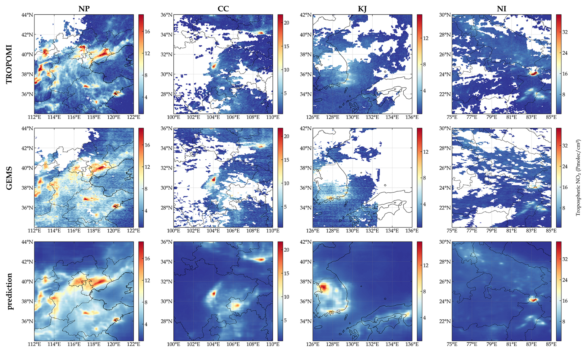
Figure 3 Comparison of single-day spatial distributions of NO₂ concentration from TROPOMI, GEMS, and model predictions on 26 April 2023.

Figure 4 shows the complete hourly GEMS observations and model predictions from 23:00 (UTC) on 9 January 2023 to 08:00 (UTC) on 10 January 2023, clearly demonstrating that the model not only has the ability to fill spatial gaps but also can predict the complete observation time series, thereby obtaining a more coherent dynamic change process.

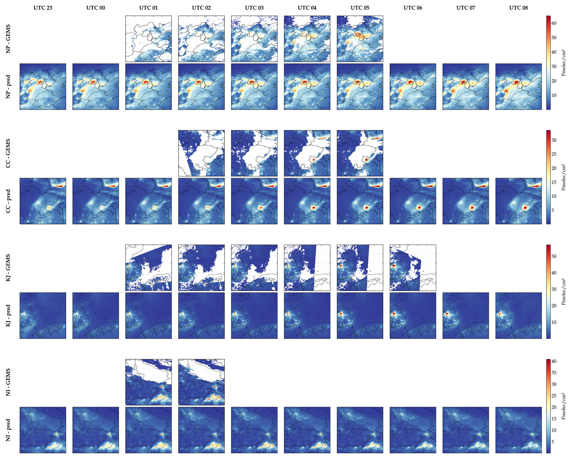
Figure 4 Hourly spatial distributions of NO₂ concentration from GEMS, and model predictions.

To assess reconstruction performance under TROPOMI input gaps, two complementary evaluations were conducted using the held-out 2023 test set. First, pixels with valid GEMS observations but missing TROPOMI inputs were evaluated, with the original TROPOMI availability mask retained during inference. The reconstruction achieved an R² of 0.801 and an RMSE of 1.235 Pmolec. cm⁻² over this subset. Second, a controlled masking experiment assessed sensitivity to spatially contiguous input gaps using 60 temporally distributed test scenes. Because GEMS serves as the supervised target and evaluation reference rather than an inference input, artificial gaps were introduced by masking originally valid TROPOMI observations within contiguous blocks and setting the corresponding validity-mask values to indicate missing inputs, while retaining all other inputs. Four block scales were tested: 0.25, 0.5, 1, and 2°. For the scenes eligible at all four scales, predictions within the artificially masked areas were evaluated against valid co-located GEMS observations. Relative to the corresponding unmasked predictions at the same locations, the RMSE increased by 0.015 Pmolec. cm⁻² (1.2 %), 0.853 Pmolec. cm⁻² (35.6 %), 1.327 Pmolec. cm⁻² (64.9 %), and 0.723 Pmolec. cm⁻² (40.7 %), respectively. These results indicate a small performance loss for the 0.25° gaps and greater degradation for the larger tested gaps, although the response was not monotonic with gap size. Together, these evaluations quantify reconstruction performance under naturally occurring and artificially imposed TROPOMI input gaps where valid GEMS references are available. Reconstructed pixels where GEMS itself is unavailable cannot be directly verified against GEMS. Therefore, these results should not be interpreted as pixelwise validation of the entire gapless product.

To further validate the model's temporal extrapolation capability and long-term application potential, this study applied the model to the data of 2024, which was not involved in any training phase, for independent validation. The performance was compared by region with that of 2023, and the results are shown in Table 3.

Table 3 Comparison of model performance on 2023 and 2024 datasets by region.

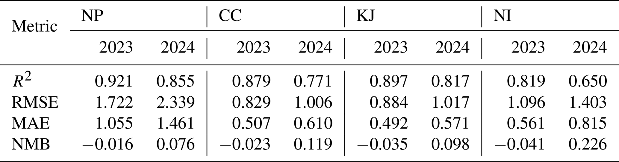
The 2024 evaluation produced lower R² values and higher RMSE and MAE values than the internal 2023 test set but retained predictive skill in all four regions, with R² values above 0.81 in NP and KJ. These results indicate that the learned relationships remain partly transferable to an unseen year, although performance varied by region and decreased most in NI. Notably, the NMB changed from negative values in all four regions in 2023 (−0.041 to −0.016) to positive values in all four regions in 2024 (0.076 to 0.226), indicating a consistent positive mean bias in the independent-year evaluation. Because the model was trained on 2023 data and the normalization statistics for the dynamic variables were derived from that training set, this sign reversal may reflect an interannual shift in the predictor-target relationship relative to the training distribution; however, evaluation of only one unseen year is insufficient to establish persistent temporal drift. The comparatively larger decrease in NI may be partly associated with the smaller number of valid GEMS labels available for this region, which provides less information for model training. Overall, the 2024 results support partial temporal transferability of the proposed framework while revealing a year-dependent bias that should be considered when applying it to longer-term historical reconstruction.

4.2 Assessment of spatial hotspot capture and historical reconstruction capability using GOME-2

In order to evaluate the hotspot reconstruction capability and historical prediction accuracy of the dataset predicted by PhysNorm-Net, this section introduces the GOME-2 instrument as a completely independent reference object. Although GOME-2C is independent of model training, it is not a retrieval-harmonized reference. Differences in AMF formulation, a priori NO₂ profiles, cloud treatment, viewing geometry, and spatial sampling among GOME-2C, GEMS, and TROPOMI may introduce systematic differences among the retrieved tropospheric NO₂ VCDs. The following cross-satellite comparisons are therefore interpreted primarily as an assessment of consistency in spatial patterns and variability, rather than as an estimate of an absolute sensor-independent NO₂ scale.

Figure 5 presents selected examples of morning NO₂ spatial distributions across the four study regions. In the selected NP case, both the reconstruction and GOME-2C observations show an extensive area of elevated NO₂ over the North China Plain, with finer spatial structures visible in the reconstruction and available GEMS observations. In the CC case, enhanced columns around Chengdu, Chongqing, and the northeastern part of the domain are evident in both the reconstruction and satellite observations, although their magnitudes and spatial extents differ. In the KJ case, the reconstruction captures enhancements over western and southern South Korea that are also apparent in the available GEMS observations, whereas GOME-2C shows a smoother distribution and a weaker enhancement near Seoul. In the NI case, both the reconstruction and GOME-2C indicate elevated columns in the southeastern part of the domain, while differences remain in the intensity and extent of individual features. These cases illustrate the reconstruction's ability to represent broad regional pollution patterns, while also revealing differences among the reconstructed fields and satellite observations.

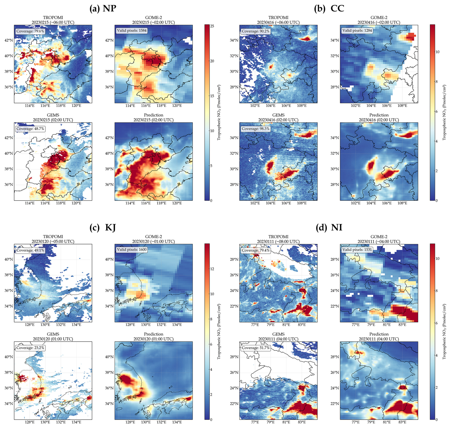
Figure 5 Comparison of tropospheric NO₂ spatial distributions from TROPOMI, GOME-2C, GEMS, and model predictions. GEMS and predictions are shown at the hourly time corresponding approximately to the GOME-2C overpass; TROPOMI observations are shown at their own overpass times.

Figure 6 displays the validation results of the predictions and original GEMS against GOME-2C from 2019 to 2024, across the four study regions and at the combined all-region scale. Since GEMS data are only available for 2023–2024, the comparison for 2019–2022 is only shown for predictions versus GOME-2C.

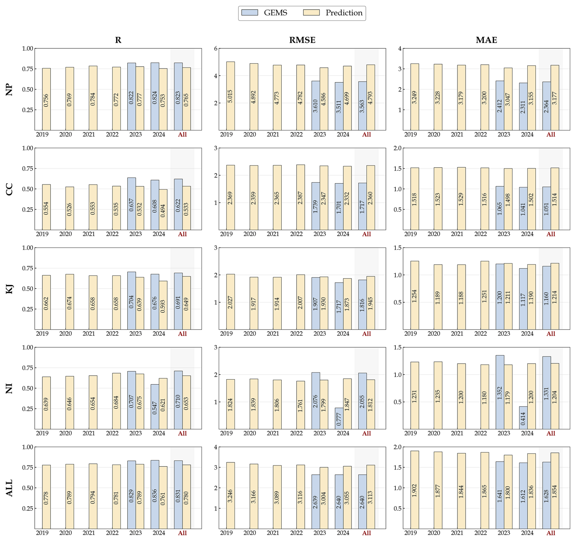
Figure 6 Annual and overall validation results of GEMS and predictions against GOME-2C for each region.

At the all-region scale, the predictions exhibit good inter-annual stability from 2019 to 2024. The annual R for the four combined regions ranges from 0.76 to 0.79, with the RMSE stable within 3.00–3.25 Pmolec. cm⁻², and the MAE maintained between 1.80 and 1.90 Pmolec. cm⁻². For the entire six-year period, the overall statistics for predictions against GOME-2C are R= 0.780, RMSE = 3.113 Pmolec. cm⁻², and MAE = 1.854 Pmolec. cm⁻². Notably, during the 2019–2022 retrospective period, the overall correlation and error levels are comparable to those of 2023–2024, indicating that the dataset predicted by the model has good stability in temporal extrapolation and does not show significant performance degradation when backtracking to non-training years.

At the regional scale, different regions exhibit clear differences. The NP region shows the highest correlation, with a six-year combined R of 0.765 for the predictions, but it also has the largest error magnitude, with RMSE and MAE of 4.794 and 3.177 Pmolec. cm⁻², respectively. This suggests that the dataset can effectively capture the dominant structure of NO₂ spatial variations in the North China Plain but is accompanied by larger absolute errors in the context of high values and strong gradients. In contrast, the CC region exhibits the lowest correlation, with a multi-year combined R of only 0.533 for the predictions, while its RMSE and MAE are 2.360 and 1.514 Pmolec. cm⁻², respectively. This indicates that although the absolute error is not high, the spatial consistency is relatively weak in this region. The KJ and NI regions have relatively low overall error levels. The predicted RMSE and MAE for the KJ region are 1.945 and 1.214 Pmolec. cm⁻², and for the NI region, they are 1.812 and 1.204 Pmolec. cm⁻². The R for both regions is approximately 0.65, indicating that the dataset maintains a relatively stable fitting ability in low-to-medium concentration backgrounds.

In the 2023–2024 period when GEMS observations are available, Fig. 6 further validates the high consistency and comparability between the predictions and the GEMS products. At the all-region scale, the correlation of GEMS with GOME-2C (R= 0.829–0.836) indeed shows a slight advantage, while the predictions' R value for the same period also reaches a high level of 0.761–0.789. This demonstrates that the output dataset has successfully internalized and inherited the capability of GEMS data to capture large-scale NO₂ spatial variability. A detailed regional comparison further highlights the robust performance of the predictions across different pollution backgrounds. In KJ, the performance gap between predictions and GEMS is minimized, with very close RMSE (approx. 1.87–1.93 vs. 1.72–1.91 Pmolec. cm⁻²) and MAE values. In NI, the predictions also show excellent reliability: in 2023, its RMSE (1.799 Pmolec. cm⁻²) and MAE (1.179 Pmolec. cm⁻²) were both lower than those of GEMS for the same period (RMSE = 2.076 Pmolec. cm⁻², MAE = 1.352 Pmolec. cm⁻²).

Overall, the independent validation based on GOME-2C demonstrates that the predictions from PhysNorm-Net can stably maintain a high overall correlation and a relatively controlled level of error during the 2019–2024 period. Furthermore, it did not show significant performance degradation in the retrospective years without GEMS label support. This indicates that the reconstructed dataset not only effectively inherits the spatiotemporal distribution information from GEMS but also has the potential for extension to historical periods, providing a reliable foundation for constructing long-term, hourly tropospheric NO₂ datasets.

4.3 Evaluation against ground-based Pandora observations

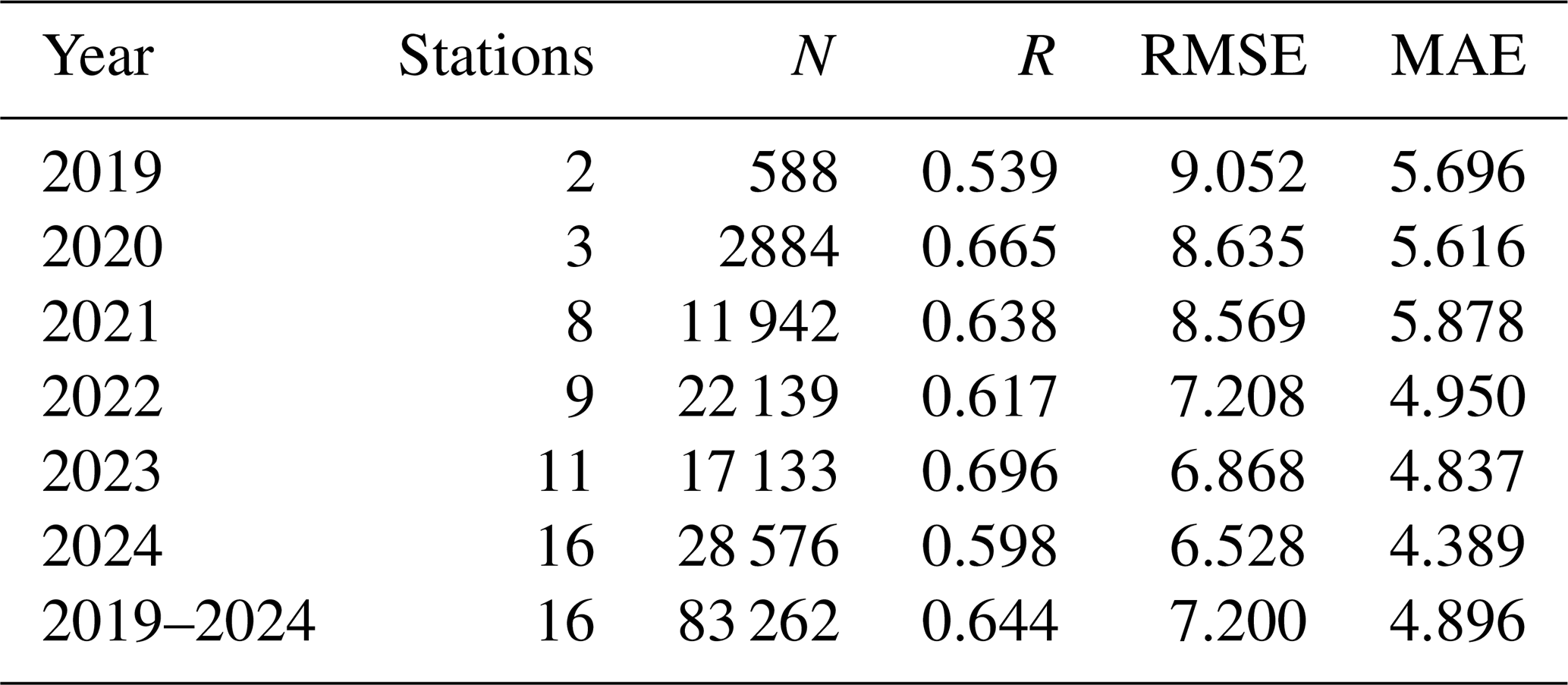
Valid Pandora observations collected within ±30 min of each hourly product timestamp were averaged and matched to the nearest 0.05° grid cell. Each hourly average required at least one valid Pandora observation, and each station contributed at most one sample per hour. Comparisons used finite positive product values. Annual and combined R, RMSE, and MAE were calculated from the collocated station-hour pairs. Reconstructed values were also evaluated separately where the corresponding GEMS scene was present but the collocated pixel lacked a valid observation.

The evaluation yielded 83 262 collocated station-hour pairs across 16 stations during 2019–2024 (Table 4). The combined R, RMSE, and MAE were 0.644, 7.200, and 4.896 Pmolec. cm⁻², respectively. Annual R ranged from 0.539 to 0.696, while RMSE ranged from 6.528 to 9.052 Pmolec. cm⁻². These comparisons extend the ground-based assessment to the historical reconstruction period and to hours without valid GEMS observations. However, the number of contributing stations increased from two in 2019 to 16 in 2024. Differences among annual statistics therefore reflect changes in station composition and observational coverage as well as reconstruction performance, and should not be interpreted as a temporal trend in product accuracy.

Table 4 Annual and combined evaluation of the reconstructed NO₂ product against Pandora observations during 2019–2024.

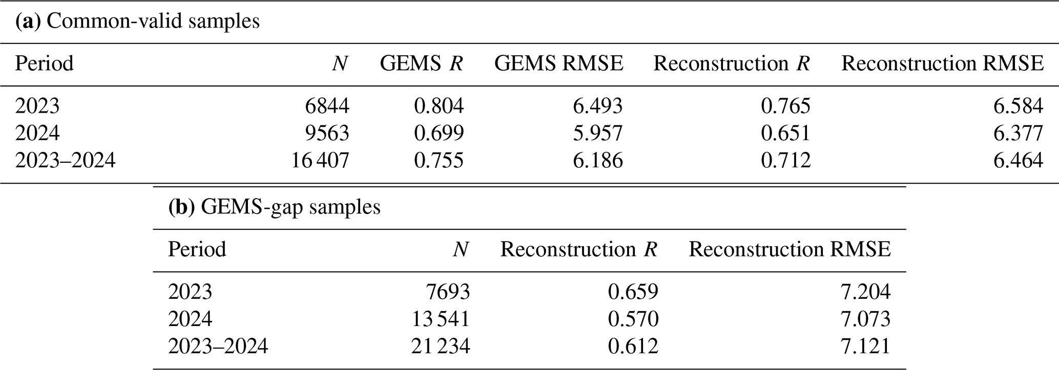
For 2023–2024, GEMS and the reconstruction achieved R values of 0.755 and 0.712, respectively, against Pandora on 16 407 common-valid samples, with corresponding RMSE values of 6.186 and 6.464 Pmolec. cm⁻² (Table 5). On the 21 234 samples where the collocated GEMS pixel lacked a valid observation, the reconstruction achieved R=0.612 and RMSE = 7.121 Pmolec. cm⁻². The correlations for these gap-filled samples were 0.659 in 2023 and 0.570 in 2024, compared with Pandora–GEMS correlations of 0.804 and 0.699 on the respective valid-GEMS subsets. The lower combined correlation and higher RMSE for the gap-filled samples indicate reduced agreement under these sampling conditions. However, the subsets differ in observational conditions, so these differences cannot be attributed solely to gap filling. The station-based results also do not establish uniform accuracy across all reconstructed pixels or study regions.

Table 5 Evaluation against Pandora observations during 2023–2024: (a) comparison of GEMS and the reconstruction on common-valid samples; (b) evaluation of the reconstruction where collocated GEMS pixels lack valid observations.

4.4 Spatiotemporal analysis of the dataset predicted by PhysNorm-Net

Leveraging the predicted hourly tropospheric NO₂ dataset from 2019 to 2024, this section systematically analyzes the spatiotemporal features of tropospheric NO₂ across the four study regions, focusing on diurnal variations and inter-annual evolution at different spatial scales.

Figure 7 presents the multi-year average Month-Hour 2D heatmaps of NO₂ for the four regions. In the East Asian regions (NP, CC, KJ), an NO₂ valley typically appears between 12:00 and 14:00 local time (LT), with high-value bands in the morning (around 08:00 LT) and evening (after 17:00 LT). Seasonally, they always exhibit high values in winter and low values in summer. This macroscopic feature aligns well with physical expectations: the bimodal morning and evening peaks are primarily attributed to concentrated emissions from rush-hour traffic coupled with a shallower planetary boundary layer, while the midday trough is due to strong photochemical dissociation of NO₂ induced by intense solar radiation. The NI region exhibits a seasonal phase distinct from that of East Asia, with its highest concentrations occurring not in winter but in the spring (March–May, the pre-monsoon period). This unique characteristic may reflect a combination of intense surface heating, frequent agricultural biomass burning, and potentially weakened photochemical loss due to aerosol-radiation feedback from heavy dust aerosols, collectively leading to extremely high NO₂ loads. This evolution of diurnal patterns with the seasons highlights the necessity of high-frequency and high-coverage observations for capturing complex regional pollution mechanisms.

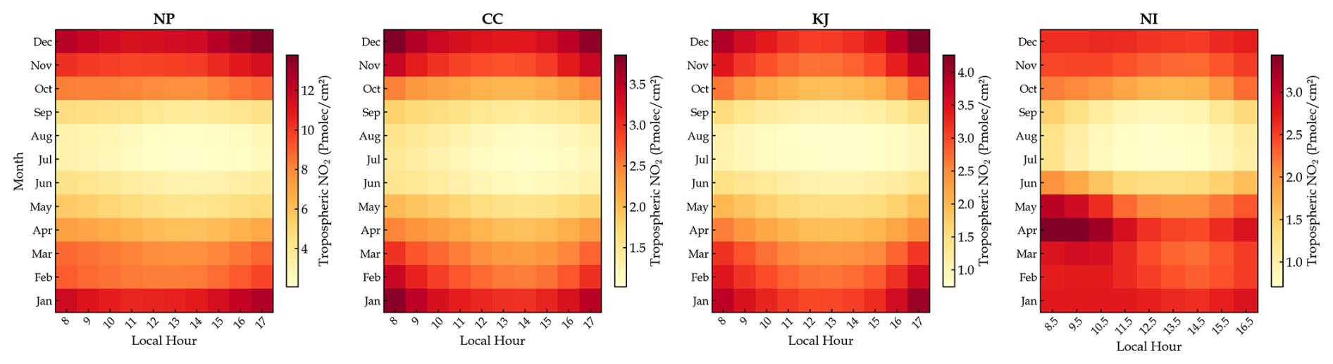
Figure 7 Month-Hour 2D distribution of tropospheric NO₂ in the four study regions from 2019 to 2024.

Beyond the regional macroscopic patterns, Fig. 8 focuses on four representative cities, including Beijing, Chengdu, Seoul, and Delhi, to reveal fine-grained diurnal structures and their inter-annual evolution under the combined influence of anthropogenic activity, atmospheric chemistry, and meteorological conditions. The diurnal amplitude in Beijing is higher in winter, whereas strong photochemical loss and deeper boundary-layer mixing suppress the overall NO₂ levels and weaken the amplitude in summer. From 2019 to 2024, the seasonal diurnal curves in Beijing show a generally parallel downward shift, indicating a sustained decrease in the reconstructed NO₂ column burden across daytime hours. Chengdu exhibits a relatively flat diurnal variation, which may be associated with the enclosed topography of the Sichuan Basin, restricted horizontal ventilation, and limited boundary-layer development. The comparatively smaller decrease in Chengdu and the temporary rebound in 2021 may reflect the combined effects of local anthropogenic activity, regional transport, and inter-annual variations in basin meteorology. Seoul exhibits an afternoon peak in winter and spring, indicating that its NO₂ burden may be influenced by regional transport from surrounding industrial areas in addition to local traffic emissions. Seoul shows the largest six-year decrease among the four cities, consistent with the declining trend recorded by the official surface NO₂ monitoring network in the Seoul metropolitan area. Delhi is strongly modulated by the South Asian monsoon system. Its diurnal amplitude is largest during the pre-monsoon spring, with high morning values followed by a sharp afternoon decrease. During the summer monsoon, daytime concentrations decline to their annual minimum under the combined effects of convective mixing, wet removal, atmospheric transport, and seasonal changes in anthropogenic and natural sources.

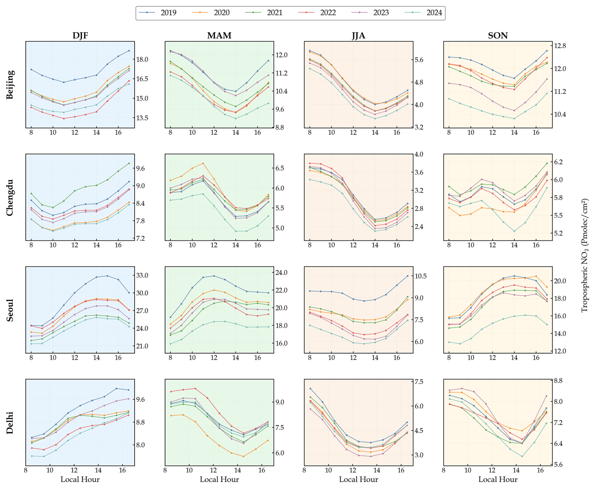
Figure 8 Inter-annual evolution of seasonal diurnal variations of tropospheric NO₂ in Beijing, Chengdu, Seoul, and Delhi from 2019 to 2024.

It should be emphasized that the inter-annual differences in the reconstructed tropospheric NO₂ VCDs should not be interpreted as direct estimates of changes in NO_x emissions. Tropospheric NO₂ columns are jointly affected by emissions, chemical lifetime, boundary-layer mixing, horizontal and vertical transport, and meteorological factors such as wind, temperature, humidity, and solar radiation (Seo et al., 2024; Yang et al., 2024; Wang et al., 2025). Accordingly, all the analyses describe inter-annual increases and decreases in the reconstructed NO₂ column burden rather than inferring direct changes in NO_x emissions. Socioeconomic activities and emission-control policies are therefore considered only as contextual information for interpreting the observed patterns. The reconstructed dataset characterizes when and where the NO₂ column burden changes, but it does not by itself quantitatively attribute those changes to specific drivers or separate policy-related effects from regional transport and meteorological variability.

Figures 9 and 10 use the hourly structure of the reconstructed dataset to compare inter-annual changes during full daytime (daily, 08:00–17:00 LT), morning (08:00–10:00 LT), midday (11:00–13:00 LT), and afternoon (14:00–17:00 LT) periods. This time-of-day-resolved analysis provides information that cannot be obtained from polar-orbiting satellite observations made at a single local overpass time. The broad 2019–2024 patterns are consistent with a recent TROPOMI-based analysis reporting substantial NO₂ VCD decreases in North and East China and South Korea, together with more heterogeneous changes across India (Huber et al., 2026).

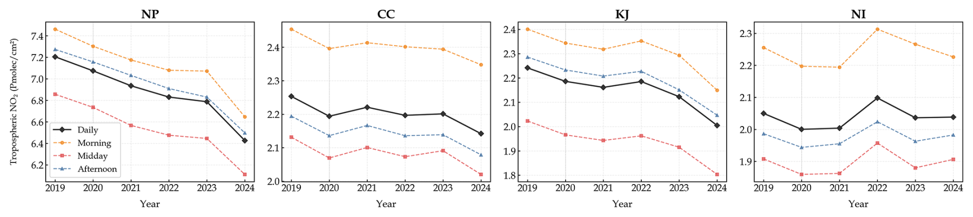
Figure 9 Inter-annual variation of tropospheric NO₂ in the four study regions during full daytime, morning, midday, and afternoon periods from 2019 to 2024.

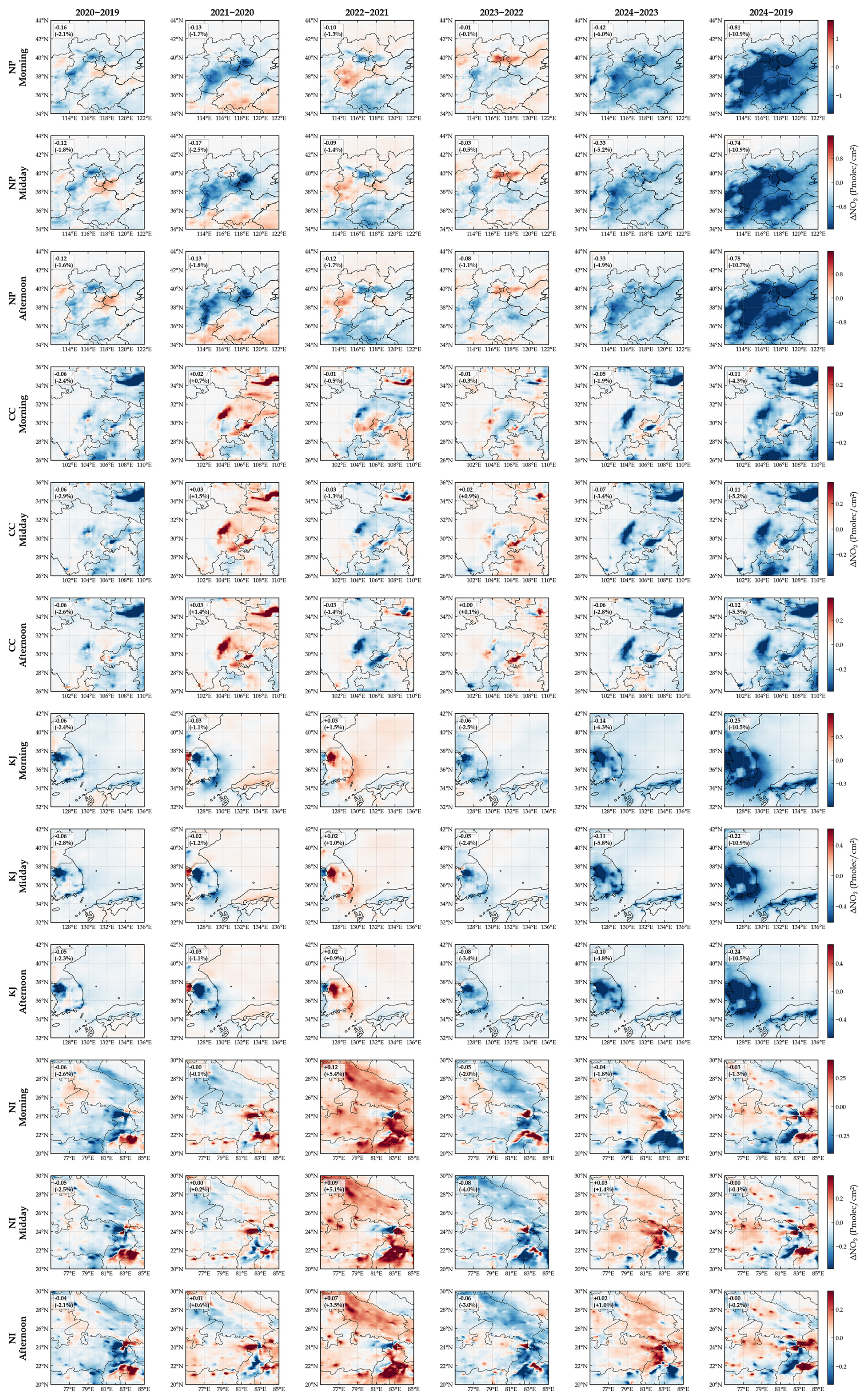
Figure 10 Spatial distribution of inter-annual differences in tropospheric NO₂ for different time slots in the four study regions from 2019 to 2024.

The NP region exhibited an overall decrease in reconstructed NO₂ VCD from 2019 to 2024 across the morning, midday, and afternoon periods. The 2019–2020 decrease was slightly larger in the morning, whereas the pronounced decrease from 2023 to 2024 occurred during all three periods. Figure 10 further shows that the strongest six-year decreases extended from the Beijing–Tianjin–Hebei urban corridor towards Shandong, with a broadly consistent spatial footprint throughout the daytime.

In the CC region, the decrease in 2020 and the subsequent rebound in 2021 occurred during all three daytime periods. Spatially, the principal urban centers, including Chengdu, Chongqing, and Xi'an, showed localized decreases, whereas several surrounding industrial and urban areas exhibited increases. In contrast to the relatively consistent daytime decrease in NP, the six-year decrease in CC was most pronounced during the afternoon.

The KJ region showed an overall decrease from 2019 to 2024 during the morning, midday, and afternoon periods, together with a modest rebound in 2022 and a pronounced decrease in 2024. Figure 10 indicates that the six-year decreases were concentrated over South Korea during all three periods, although localized inter-annual variations remained near Incheon, coastal areas, and the surrounding waters.

The NI region exhibited the most spatially heterogeneous pattern among the four study regions. Regional mean reconstructed NO₂ VCD increased markedly in 2022 during all three daytime periods and subsequently returned to approximately its 2019 level by 2024. Figure 10 reveals a complex mixture of increases and decreases along the Indo-Gangetic Plain, with clear differences in their spatial distribution among the morning, midday, and afternoon periods.

5 Discussion

5.1 Physical interpretability and feature importance analysis of PhysNorm-Net

The following diagnostics are reported to build trust in the dataset by demonstrating that the reconstruction responds to physical drivers, rather than as a stand-alone mechanistic study. This study first verified the functional integrity and physical responsiveness of the dual-branch architecture through a model diagnostic experiment (Fig. 11). The experiment compared the outputs of the normal prediction mode (using both satellite observations and physical prior inputs) with a “blind test” mode (where satellite branch inputs were zeroed out with a full missing-data mask, forcing the model to rely solely on the physical branch). This was done to examine the model's sensitivity to changes in physical inputs. The diagnostic results show that the model can still output the general distribution of NO₂ even when relying exclusively on the physical branch, which ensures predictive capability during periods without TROPOMI observations. The inclusion of the satellite branch then effectively corrects the concentration details and gradients. From a functional validation perspective, this finding confirms that the physical branch plays a primary role in providing foundational information, while the satellite branch is mainly responsible for the fine-grained refinement of high-resolution details.

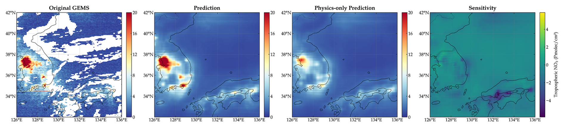
Figure 11 Functional diagnostic experiment of the PhysNorm-Net dual-branch architecture. The example shown corresponds to the KJ region at 04:00 UTC on 11 November 2024.

Building on this diagnostic foundation, to further unveil the model's decision-making mechanism, we quantitatively analyzed the relative contributions of each input variable during daytime hours in 2023 using a zero-out perturbation method (Zhang and Gao, 2020). This method calculates a variable's importance score by zeroing out its specific channel and measuring the resulting deviation from the baseline output, quantified by MAE. Figure 12 reports the three highest-ranked individual input channels for each bin. The dominant variable combinations differ significantly across the four regions, indicating that the model does not simply rely on a fixed set of factors but instead forms region-specific control structures.

Because several input variables are physically and statistically correlated, such as specific humidity and temperature across multiple pressure levels, the individual-channel scores are not additive and should not be interpreted as unique causal contributions. When correlated variables contain overlapping information, the model may compensate for the perturbation through the remaining channels, or the perturbation may disrupt information shared across several channels. Therefore, the resulting rankings represent conditional model sensitivity under the applied perturbation, rather than independent explanatory importance; the rankings in Fig. 12 are interpreted as diagnostic evidence of relative model sensitivity under the sampled 2023 conditions, and are considered together with the physical context of each region and season.

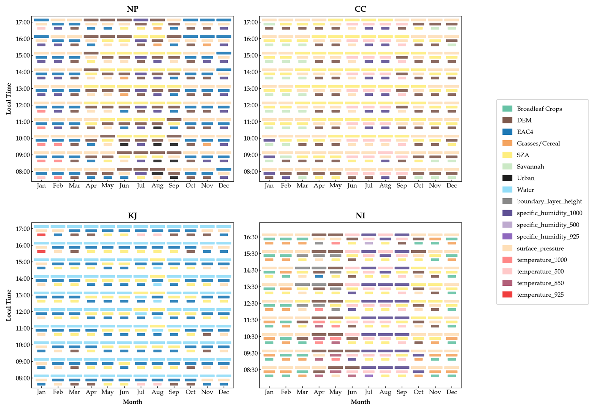
Figure 12 Monthly and hourly feature importance rankings for the four regions based on the zero-out perturbation method.

As shown in Fig. 12, in the NP region, the most stable and prominent variables during winter and late autumn are EAC4 and surface pressure, with the third position often supplemented by near-surface or mid-tropospheric thermodynamic variables. This channel-level pattern has a clear physical meaning: in East Asian winters, frequent temperature inversions, stable weather conditions, and high relative humidity collectively suppress vertical mixing and promote the accumulation of NO₂ in the near-surface layer (Chai et al., 2014; Xu et al., 2011). Concurrently, the increased importance of EAC4 during certain winter periods indicates greater model sensitivity to the large-scale chemical background represented by EAC4. In summer (JJA), SZA becomes more prominent and shows a strong daytime peak around noon. This aligns with the physical processes of enhanced convective mixing and accelerated photochemical decomposition in the warm season (Liu et al., 2022).

In the CC region, the rankings are dominated by surface pressure and SZA. Surface pressure is the top-ranked input channel throughout the daytime in winter and remains prominent during the morning and late-afternoon periods in transitional months, whereas SZA is generally top-ranked from spring to early autumn, particularly around midday. DEM frequently appears among the three highest-ranked channels outside midsummer, while the savannah land-cover channel is more prominent during colder months. During summer, the 500 hPa temperature and 1000 hPa specific humidity channels also become prominent. These seasonal and diurnal shifts indicate changes in model sensitivity between circulation and ventilation constraints and radiation and thermodynamic conditions, consistent with the meteorological characteristics of the Sichuan Basin (Sun et al., 2020; Feng et al., 2022).

In the KJ region, the water-body land-cover channel is the top-ranked variable during almost all months and daytime hours. This implies that in a peninsula-archipelago system with complex coastlines and strong land-sea segmentation, the water body variable effectively encodes the regional land-sea distribution, which in turn determines the spatial extent of emission sources and sea breeze influence. EAC4 also remains among the three highest-ranked channels in nearly all month–hour bins, generally occupying the second or third position. SZA and surface pressure account for most of the other highly ranked channels, with their prominence varying across seasons and daytime hours. Overall, the channel-level results indicate persistent model dependence on both the land-sea spatial pattern and the large-scale chemical background, together with seasonal and diurnal modulation by radiation and meteorological conditions.

The NI region exhibits a strong seasonal switch. During winter and late autumn, surface pressure is almost consistently ranked first, indicating that NO₂ distribution in this region is primarily controlled by boundary layer stability and ventilation conditions during the cold and transitional seasons. Concurrently, the land use types grasslands/cereal crops and broadleaf crops become prominent in winter. These agricultural land types are widespread in the Indo-Gangetic Plain, and their high importance reflects the impact of agricultural burning – the widespread burning of crop residues in this region is a major seasonal source of NO_x (Cusworth et al., 2018; Jethva et al., 2018). Around the monsoon season, the dominant variables shift to specific humidity, temperature, and SZA, with these thermodynamic and radiation-related channels appearing more frequently among the top-ranked variables, whereas the prominence of individual land-use channels decreases. This reflects the profound influence of monsoon dynamics on vertical mixing, wet scavenging, and the large-scale redistribution of pollutants (Ravindra et al., 2003).

The rankings in Fig. 12 quantify the model's dependence on individual input channels rather than the aggregate contributions of broader physical processes. Furthermore, the zero-out perturbation method measures model dependency rather than strict physical causality. Therefore, the importance of static variables such as land use and DEM should be interpreted as the model's reliance on spatial encoding and regional templates.

During the above feature-importance analysis, EAC4 was identified as an important chemical prior. We therefore further quantified the dependence of the reconstructed values on EAC4 using all 1450 scenes in the held-out 2023 test set. With the model weights and all other inputs fixed, the de-standardized EAC4 field was perturbed by ±20 %, and the results were pooled over GEMS-valid pixels for which the TROPOMI input was missing. The baseline reconstruction for this subset achieved R²=0.801 and an RMSE of 1.235 Pmolec. cm⁻². Increasing and decreasing EAC4 by 20 % changed the pooled mean reconstruction by +4.02 % and −4.60 %, respectively, corresponding to normalized sensitivity to EAC4 perturbations of 0.216 (estimated using a central difference as $E=\frac{{\stackrel{\mathrm{‾}}{\widehat{y}}}_{+\mathrm{20}\mathit{\%}}-{\stackrel{\mathrm{‾}}{\widehat{y}}}_{-\mathrm{20}\mathit{\%}}}{\mathrm{0.4}{\stackrel{\mathrm{‾}}{\widehat{y}}}_{\mathrm{baseline}}}$, where ${\stackrel{\mathrm{‾}}{\widehat{y}}}_{+\mathrm{20}\mathit{\%}}$, ${\stackrel{\mathrm{‾}}{\widehat{y}}}_{-\mathrm{20}\mathit{\%}}$, and ${\stackrel{\mathrm{‾}}{\widehat{y}}}_{\mathrm{baseline}}$ denote the mean reconstructed NO₂ VCD over the same pixel subset with EAC4 increased by 20 %, decreased by 20 %, and unchanged, respectively). This dimensionless metric quantifies the relative response of the pooled mean reconstruction to the imposed EAC4 perturbations, rather than prediction bias relative to GEMS. Its value of 0.216 indicates that the relative output response is approximately 21.6 % of the relative input perturbation, as estimated across the tested ±20 % range. The region-specific normalized sensitivities were 0.134, 0.269, 0.220, and 0.227 for CC, KJ, NI, and NP, respectively. This attenuated and regionally variable response indicates that EAC4 provides an important large-scale chemical constraint but is not transferred proportionally to the model output.

5.2 Limitations and future work

Although the validation results support several uses of the reconstructed dataset, users should consider the following limitations.

The training domains were selected to emphasize representative high-emission and complex-terrain regions, which increases the representation of polluted and high-gradient conditions but limits model generalizability to very clean backgrounds, such as remote oceanic regions. Uncertainty under low-column conditions also arises from treating satellite NO₂ VCD retrievals less than or equal to zero as missing values. Although this treatment is consistent with the nonnegative model domain and the logarithmic transformation, negative retrievals form part of the random retrieval-error distribution, and their exclusion may introduce an upward conditional-sampling bias near the satellite retrieval detection limit. The reported evaluations therefore characterize the positive-retrieval subset, and the product should not be interpreted as an unbiased estimate under ultra-low background conditions. Future work will examine adaptive sampling, loss weighting, sign-preserving preprocessing, and alternative transformation strategies.

The framework was trained primarily on 2023 data from four hotspot regions. Longer training records may improve robustness to extreme meteorological conditions and inter-annual shifts in the emission baseline. Because the physicochemical evolution of tropospheric NO₂ depends on local meteorology, atmospheric chemistry, transport, and emission characteristics, direct application of the model beyond the training domains may be affected by domain shift. Transfer to a new region should therefore be accompanied by region-specific validation, with fine-tuning using local reference data when performance degradation is observed. Regions characterized by substantially different emission structures, meteorological regimes, topography, or seasonal behavior may require more extensive retraining (Tiwari et al., 2026). Independent evaluation should be conducted before the reconstructed product is used for quantitative analyses in a new domain.

At the data-product level, integrating the 0.25° physical prior fields with the 0.05° observations may introduce spatial smoothing. Although this integration can suppress retrieval noise, it may also weaken localized gradients around individual emission sources. Related uncertainty arises from the EAC4 chemical prior because EAC4 tcno2 is a coarse-resolution, 3-hourly total-column quantity, whereas the target is an hourly tropospheric VCD. The column-type mismatch may transmit EAC4 background or stratospheric biases into the reconstruction, while linear temporal interpolation may smooth rapidly evolving chemical features between EAC4 analysis times. These effects are expected to be most relevant where TROPOMI information is absent or sparse. Future work will examine higher-temporal-resolution and vertically resolved tropospheric chemical priors and methods that explicitly represent uncertainties associated with temporal interpolation and column-type mismatch.

Independent evaluation of the 2019–2022 historical reconstruction remains limited by the temporal and spatial coverage of the reference observations. GOME-2C provides a satellite comparison near its approximately 09:30 LT overpass, while Pandora supplies additional hourly comparisons at the available ground stations. However, Pandora coverage is concentrated in KJ, with limited coverage in NP and NI and no eligible station in CC in this evaluation. These observations therefore do not provide comprehensive validation of daytime variability throughout all study domains. Cross-sensor retrieval differences add further uncertainty because the TROPOMI input, GEMS training target, and GOME-2C external reference differ in their retrieval configurations, observation times, and spatial sampling. Differences in AMF formulation, a priori NO₂ profiles, cloud treatment, viewing geometry, and spatial footprints may affect both the relationship learned between TROPOMI and GEMS and the discrepancies observed in the GOME-2C evaluation. Future work will assess cross-sensor consistency using retrieval-harmonized products or comparison approaches that explicitly account for these differences. The continued operation of GEMS, TEMPO, and Sentinel-4 will also provide opportunities to examine cross-sensor transferability and extend the framework to broader daytime-hourly NO₂ applications.

6 Data availability

TROPOMI is available at https://doi.org/10.5270/S5P-9bnp8q8 (Copernicus Sentinel-5P, 2021). GEMS data can be accessed at https://nesc.nier.go.kr/en/html/datasvc/data.do?pageIndex=1&outputInnb=64&atrb=NO2_Trop (last access: 9 June 2026). The GOME-2 data are provided by the EUMETSAT AC-SAF as described in https://acsaf.org/products/nto_no2.php (last access: 9 June 2026). Pandora rnvh3p1-8 observations are available from the Pandonia Global Network through https://api.pandonia-global-network.org/docs (last access: 9 June 2026). ERA5 on single and pressure levels can be accessed at https://doi.org/10.24381/cds.adbb2d47 (Copernicus Climate Change Service, 2023a) and https://doi.org/10.24381/cds.bd0915c6 (Copernicus Climate Change Service, 2023b), respectively. EAC4 data can be accessed at https://doi.org/10.24381/d58bbf47 (Copernicus Atmosphere Monitoring Service, 2020). MCD12C1 data is available at https://doi.org/10.5067/MODIS/MCD12C1.061 (Friedl and Sulla-Menashe, 2022). ETOPO data can be found at https://doi.org/10.25921/FD45-GT74 (NOAA National Centers for Environmental Information, 2022). The gapless 0.05° daytime-hourly tropospheric NO₂ dataset (2019–2024) produced in this study is available at https://doi.org/10.5281/zenodo.20427767 (Gao et al., 2026).

7 Conclusions

This study presents the first seamless, 0.05° daytime-hourly tropospheric NO₂ vertical column density dataset covering typical Asian hotspots from 2019 to 2024. To overcome the core challenges of spatial discontinuity and short historical records inherent in high-frequency geostationary satellite data, this dataset was reconstructed using an advanced physics-aware deep learning framework (PhysNorm-Net).

The high quality and physical reliability of this dataset are ensured through a rigorous multi-modal fusion mechanism. First, this study utilizes a Partial Convolutional network with dynamic mask updates to effectively isolate mean-value contamination from invalid pixels, enabling the precise extraction of high-resolution spatial textures. Second, deviating from traditional channel-wise concatenation, the PhysNorm module uses multi-level meteorological, topographical, and chemical prior fields as environmental context to adaptively control the affine transformation of high-resolution features. This ensures that the reconstructed concentration fields strictly adhere to the physical laws of advection-diffusion and photochemical reactions. Third, the loss function adopts a combination of fine-grained reconstruction and coarse-grained physical consistency constraints to further mitigate the gradient dilution problem in deep networks.

Quantitative assessments confirm that the reconstructed dataset achieves extremely high fitting accuracy on the test set (R²= 0.889) and can effectively recover morning and evening pollution hotspots missed by polar-orbiting instruments like TROPOMI due to their spatiotemporal coverage limitations. More importantly, the long-term retrospective validation against GOME-2C data (R=0.780), not used in the PhysNorm-Net training, demonstrates that the dataset possesses robust temporal stability and high fidelity in historical periods (2019–2022) prior to the operational deployment of GEMS. Pandora observations provide additional ground-based evaluation during the historical reconstruction period, although their uneven station coverage, together with the restricted overpass sampling of GOME-2C, limits comprehensive validation of daytime variability across all study domains.

Through in-depth analysis, this newly generated long-term hourly dataset has proven its unique scientific utility in capturing complex atmospheric dynamics. It not only clearly reveals the monsoon-driven seasonal phase reversal in North India and the typical bimodal and single-trough diurnal pattern in East Asia, but also characterizes the sustained decreases in reconstructed NO₂ in the North China Plain and the Korea-Japan region since 2019, together with localized inter-annual rebounds in specific years (e.g., 2021). By combining sparse satellite retrievals with continuous physical priors, the dataset provides a continuous record that can support studies of long-term air pollution variability, health exposure, and epidemiological applications across the four study regions.