Ise Bay Reanalysis (IBRA): a 12-year ecological hydrodynamic reanalysis dataset for Ise Bay, Japan

Reanalysis datasets based on coupled ocean circulation and ecosystem models are essential tools for understanding coastal environmental variability and supporting water-quality management. However, the development of such datasets for semi-enclosed coastal systems remains limited, particularly for those incorporating subsurface biogeochemical observations such as dissolved oxygen (DO). This study presents the Ise Bay Reanalysis (IBRA), a high-resolution, 12-year (2011–2022) reanalysis dataset of hydrodynamic and biogeochemical variables for Ise Bay, Japan. The dataset was generated using the Ecological hydrodynamics simulation system of the Port and Airport Research Institute Simulator (EcoPARI-Simulator), coupled with an ensemble Kalman filter data assimilation system that assimilated in situ observations of water temperature, salinity, and bottom-layer DO at 6 h intervals. The resulting dataset has an hourly temporal resolution and resolves the entire water column. IBRA has three key distinguishing features. First, unlike many previous reanalysis datasets that rely primarily on satellite observations, IBRA assimilates continuous in situ measurements throughout the water column, including high-frequency DO observations, thereby improving the representation of subsurface dynamics. Second, the 6 h assimilation cycle enables the dataset to resolve short-term variability driven by tidal processes, which are a dominant control of coastal transport and mixing. Third, spatially coherent corrections are applied across the entire bay using an ensemble Kalman filter, ensuring spatial consistency in both physical and biogeochemical fields while avoiding artificial discontinuities often associated with simpler data assimilation approaches. The quality of IBRA was evaluated using statistical metrics and detailed comparisons against in situ observations. Data assimilation improved overall agreement with observations across multiple stations and depths, particularly for bottom-layer DO concentrations. The dataset successfully reproduced seasonal variability, vertical stratification, and the formation and persistence of hypoxic conditions in the inner bay, while also capturing well-oxygenated conditions near the bay mouth. Furthermore, the spatial distributions of temperature, salinity, and DO were realistically represented, including the intrusion of offshore water masses and associated horizontal gradients. The IBRA dataset therefore provides a dynamically consistent and comprehensive representation of physical and biogeochemical variability in a semi-enclosed coastal system. It is expected to serve as a valuable resource for studies of coastal hypoxia, water-quality assessment, and environmental management. The IBRA dataset is publicly available via Zenodo at https://doi.org/10.5281/zenodo.19808667 (Matsuzaki et al., 2026).

1 Introduction

Model systems that combine realistic representations of ocean circulation with biogeochemical or ecosystem models are valuable tools for analysis and prediction (Fennel et al., 2019). Accordingly, the demand for reanalysis datasets based on coupled hydrodynamic–ecosystem models has increased for assessing marine environmental variability and long-term change (Von Schuckmann et al., 2018), and several advanced studies have been conducted in this field. For example, Ford and Barciela (2017) developed a global marine biogeochemical reanalysis for the period from 1997 to 2012 by assimilating ocean-color-derived chlorophyll observations into a physical–biogeochemical ocean model. Ciavatta et al. (2018) performed a reanalysis of the northeast Atlantic, including the northwest European continental shelf, covering the period from 1998 to 2003, by assimilating phytoplankton functional types derived from ocean color observations into an ecosystem model. Cossarini et al. (2021) developed a reanalysis product for the Mediterranean Sea spanning the period from 1999 to 2019 at a horizontal grid resolution of $\mathrm{1}/\mathrm{24}$°. Chamberlain et al. (2021) presented BRAN2020, a near-global eddy-resolving ocean reanalysis spanning 1993–2019 at a horizontal resolution of $\mathrm{1}/\mathrm{10}$°.

These previous studies have relied primarily on satellite-derived data, which are largely limited to the sea surface; consequently, their ability to resolve subsurface biogeochemical variability remains limited. In semi-enclosed coastal systems, complex interactions among tides, stratification, and biogeochemical processes generate greater spatiotemporal variability than is typically seen in the open ocean. Regional coastal reanalysis studies have also been conducted using data-assimilation models. For example, Wilkin et al. (2022) developed a data-assimilative circulation reanalysis for the U.S. Mid-Atlantic Bight and the Gulf of Maine using the Regional Ocean Modeling System with four-dimensional variational data assimilation, incorporating satellite, coastal radar, and in situ data. However, these studies have primarily focused on physical ocean circulation, and applications incorporating fully coupled ecosystem processes remain limited. Therefore, the assimilation of subsurface observational data is particularly important for semi-enclosed coastal systems. These factors make reanalysis efforts in such environments particularly challenging. To the best of our knowledge, reanalysis datasets that directly assimilate oxygen data remain relatively rare. In Japan, the Ministry of the Environment has been gradually establishing environmental standards for bottom-layer dissolved oxygen (DO) concentrations in enclosed water bodies and lakes. Therefore, understanding the spatiotemporal distribution of bottom-layer DO is expected to become increasingly important from both scientific and policy perspectives.

In this study, we developed the Ise Bay Reanalysis (IBRA), a 12-year (2011–2022) reanalysis dataset of hydrodynamic and aquatic ecosystem variables for Ise Bay, Japan, using the numerical model (Matsuzaki et al., 2024; Tanaka and Suzuki, 2010; Tanaka et al., 2011) and the data assimilation system (Matsuzaki and Inoue, 2022) of the Ecological hydrodynamics simulation system of the Port and Airport Research Institute (EcoPARI). The dataset presented here extends the existing hydrodynamic reanalysis dataset (Matsuzaki et al., 2025a) by coupling an ecosystem model with the assimilation of bottom-layer DO observations. The development of IBRA was motivated by the designation of water quality classifications based on bottom-layer DO concentrations in Ise Bay and is intended to provide scientific information to support assessments of compliance with these environmental quality standards.

The IBRA dataset has three key features. First, it assimilates continuous in situ observations throughout the entire water column, including bottom-layer DO measurements. Second, observations are assimilated every 6 h, enabling the representation of short-term variability associated with tidal processes. Third, data assimilation is performed using an ensemble Kalman filter (EnKF), which provides spatially consistent corrections throughout the bay. Further details are presented in Sect. 2.

This study describes the development of IBRA and evaluates its applicability using quantitative accuracy metrics and qualitative comparisons against observed spatial distributions. The remainder of this paper is organized as follows: Sect. 2 describes the hydrodynamic–ecosystem model, the data assimilation system, and the observational data assimilated. Section 3 presents the quality evaluation of the reanalysis dataset. Section 4 discusses the three distinguishing features of the reanalysis dataset. Section 5 describes the available data outputs, data access methods, and file organization. Section 6 presents the main conclusions, potential applications of IBRA, and final remarks.

2 Materials and methods

2.1 Simulation model and setup

The simulation model and its setup were adapted from previously reported configurations (Matsuzaki and Inoue, 2022; Matsuzaki and Kubota, 2024; Matsuzaki et al., 2025b). The model domain encompasses Ise Bay (Fig. 1), with an area of 2342 km², a volume of 3.94 × 10¹⁰ m³, an average depth of 17 m, and a maximum depth of 100 m (https://www.cbr.mlit.go.jp/kikaku/sai_ise/pdf/koudou_01.pdf, last access: 25 March 2026). The bay is located in the south-central part of Honshu Island, Japan, and extends approximately 70 km in both the north–south and east–west directions. Its open boundary connects to the Pacific Ocean, and the annual river discharge is 2.0 × 10¹⁰ m³, which is approximately one-half of the volume of Ise Bay. Ise Bay receives river inflows from 10 Class A rivers (Table S4 in the Supplement) and 76 smaller tributaries. The Kiso, Ibi, and Nagara rivers, which provide the largest discharges, enter the inner part of the bay (Fig. 1). Seasonal wind patterns include northwesterly winds from autumn to spring, whereas sea and land breezes predominate in summer, blowing from the southeast during the day and from the northwest at night (Sekine et al., 2002).

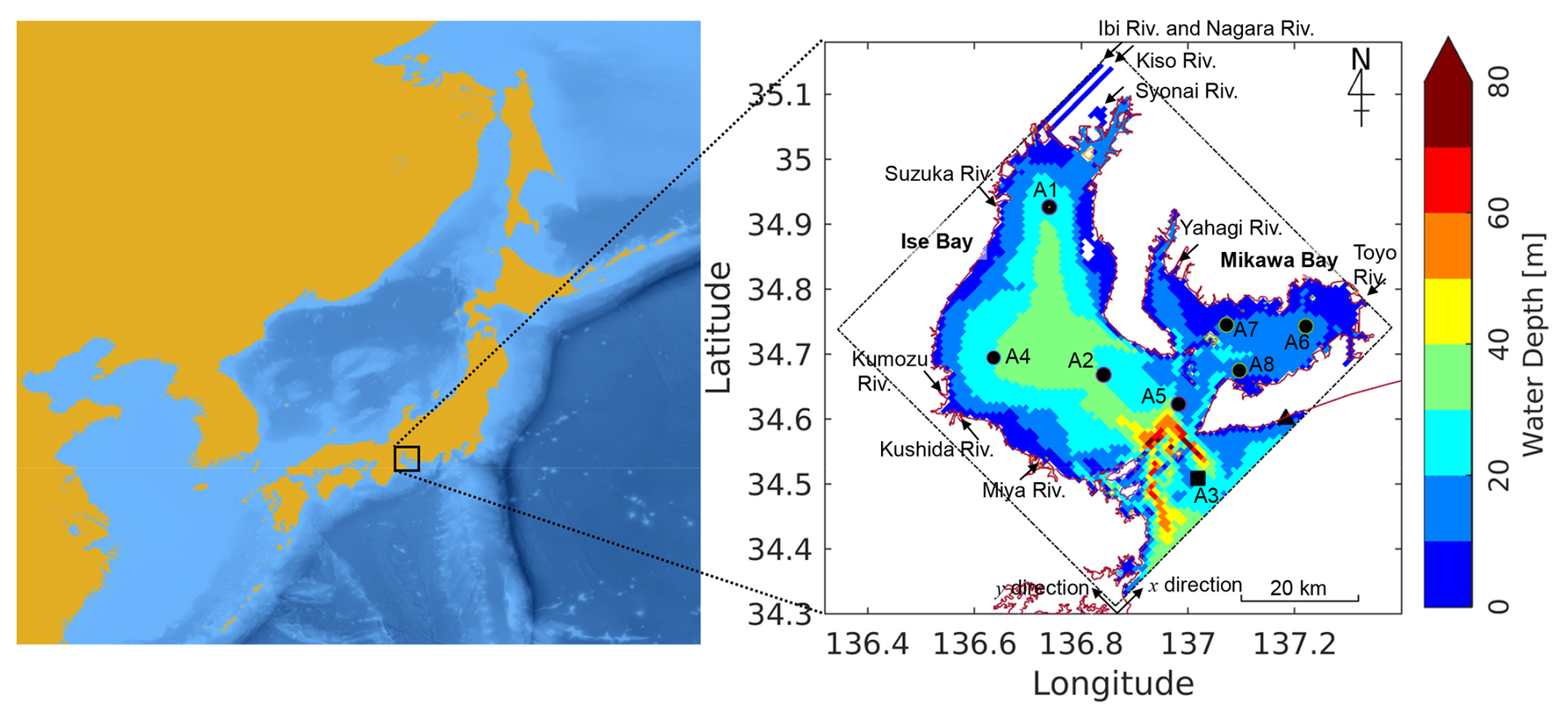
Figure 1 Location maps of Japan and the Pacific coast of East Asia (left) and Ise Bay (right). The dash-dotted line represents the computational domain for the numerical model and the data assimilation system. The circles and square indicate the observation points used for data assimilation. The square indicates the observation point used to prescribe the lateral boundary conditions for water temperature and salinity. The triangle denotes the observation point used to prescribe the lateral boundary condition for tidal elevation. Water depth is indicated by color in the map. Arrows show the inflow locations and flow directions of the 10 Class A rivers. The northeast and northwest axes indicate the computational grid in the x- and y-directions, with a grid size of 85 × 85 and a grid spacing of 800 m. Basemap for the left panel: Bathymetry data were obtained from the GEBCO_2026 Grid (GEBCO Bathymetric Compilation Group, 2026), and the map was generated using QGIS.

Simulations were conducted using the EcoPARI-Simulator: Ecological hydrodynamics simulation system of the Port and Airport Research Institute (Matsuzaki et al., 2024; Tanaka and Suzuki, 2010; Tanaka et al., 2011). EcoPARI-Simulator uses a Cartesian coordinate system to simulate coastal and estuarine circulation dynamics. The horizontal resolution in both the x and y directions (800 m) was determined through a trade-off between accurately representing bathymetry at the mouth of Ise Bay and reducing computational costs. The coordinate system was rotated 45° clockwise, and a z-coordinate system was adopted for the vertical direction. The vertical grid comprised 38 layers, with layer spacings of 0.5 m from the surface to 4 m, 1 m from 4 to 11 m, 2 m from 11 to 41 m, 9 m from 41 to 50 m, 20 m from 50 to 70 m, and 30 m from 70 to 100 m. Bathymetric data were obtained directly from the Japan Coast Guard. A subgrid-scale model (Smagorinsky, 1963) was used as the horizontal turbulence model, and the model proposed by Munk and Anderson (1948) was used as the vertical turbulence closure. The Sommerfeld radiation condition was applied as the open-boundary condition at the lateral boundary (Orlanski, 1976). The governing equations for water temperature, salinity, and DO used in this study were scalar transport equations, the details of which are described in previous studies (Hafeez et al., 2021; Matsuzaki et al., 2025b; Tanaka and Suzuki, 2010; Tanaka et al., 2011).

2.2 Boundary condition settings

Three types of boundary conditions were specified: lateral, atmospheric, and river-discharge conditions. The lateral boundary conditions for seawater temperature and salinity were derived from observational data obtained near the open boundary (black square in Fig. 1). In addition, observed water-level data at a station near the lateral boundary (black triangle in Fig. 1) were prescribed as boundary conditions. Atmospheric forcing data were obtained from two datasets: (i) the Japan Meteorological Agency's Grid Point Value of the Meso-scale Model (GPV-MSM) for the simulation period from 1 January 2011 to 31 December 2016; and (ii) the Japan Meteorological Agency's Grid Point Value of the Local Forecast Model (GPV-LFM; https://www.jma.go.jp/jma/kishou/know/whitep/1-3-6.html, last access: 17 March 2026) for the simulation period from 1 January 2017 to 31 December 2022. These two datasets were used because the GPV-LFM has been available only since January 2016, whereas prior to that, only the GPV-MSM dataset was available. River discharge boundary conditions were specified using available observational data. Further details on the boundary condition settings are provided in the Supplement.

2.3 Assimilation model

The assimilation model and its setup were adapted from previously reported configurations (Matsuzaki and Inoue, 2022). The EnKF model for the Ise Bay Simulator was implemented following the approach described by Evensen (2003). The fundamental analysis procedures of the Kalman filter and EnKF are described below. The analysis value x^a (data assimilation result) at time t is obtained as the optimal weighted average of the background value x^f (forecast/simulation result) and the observed value y, as shown in Eq. (1):

$$\begin{array}{}\text{(1)}& {\mathit{x}}_t^{\mathrm{a}}={\mathit{x}}_t^{\mathrm{f}}+{\mathbf{K}}_t\left({\mathit{y}}_t-{\mathbf{H}}_t{\mathit{x}}_t^{\mathrm{f}}\right)\end{array}$$

where x represents the state vector, whose elements are physical and ecosystem variables, such as water temperature, salinity, current velocity, phytoplankton concentration, and DO concentration at each grid cell in the numerical model; y is the observation vector, whose elements are the observed values for water temperature, salinity, and DO; H is the observation operator that extracts the physical and ecosystem variables from the grid cell corresponding to each observation location in the numerical model state vector; and K is the Kalman gain, which determines the degree to which the observations are assimilated. K is calculated as follows:

$$\begin{array}{}\text{(2)}& {\mathbf{K}}_t={\mathbf{P}}_t^{\mathrm{f}}{\mathbf{H}}_t^T{\left({\mathbf{R}}_t+{\mathbf{H}}_t{\mathbf{P}}_t^{\mathrm{f}}{\mathbf{H}}_t^T\right)}^{-\mathrm{1}}\end{array}$$

where P is the background error covariance matrix, R is the observation error covariance matrix, and the superscript T denotes the transpose. Equation (2) shows that the degree to which observations are assimilated is determined by the relationship between P and R, whereas the spatial extent of the corrections introduced by the observations is determined by P. As mentioned in the Introduction, the main objective of this study is to generate appropriate ensembles for regional coastal and estuarine modeling, which depends on the background error covariance matrix P. The data assimilation procedure using the EnKF is as follows:

• a.

  Ensemble members were generated using the EcoPARI-Simulator numerical model. In this study, the ensemble members were generated under varying boundary conditions and model parameters, as described in Sect. 2.4. The total number of ensemble members is denoted by L.

• b.

  The background error covariance matrix is estimated based on the ensemble members.

  $$\begin{array}{}\text{(3)}& {\displaystyle }{\stackrel{\mathrm{‾}}{\mathbf{P}}}_t^{\mathrm{f}}={\displaystyle \frac{\mathrm{1}}{L-\mathrm{1}}}{\sum }_{l=\mathrm{1}}^L\left({\mathit{x}}_t^{\mathrm{f}\left(l\right)}-{\stackrel{\mathrm{‾}}{\mathit{x}}}_t^{\mathrm{f}}\right){\left({\mathit{x}}_t^{\mathrm{f}\left(l\right)}-{\stackrel{\mathrm{‾}}{\mathit{x}}}_t^{\mathrm{f}}\right)}^T\text{(4)}& {\displaystyle }{\stackrel{\mathrm{‾}}{\mathit{x}}}_t^{\mathrm{f}}={\displaystyle \frac{\mathrm{1}}{L}}{\sum }_{l=\mathrm{1}}^L{\mathit{x}}_t^{\mathrm{f}\left(l\right)}\end{array}$$

  Here, ${\stackrel{\mathrm{‾}}{\mathit{x}}}_t^{\mathrm{f}}$denotes the ensemble mean, and the overbar indicates the ensemble average.

• c.

  The observation error covariance matrix is estimated based on the ensemble members.

  $$\begin{array}{}\text{(5)}& {\displaystyle }{\stackrel{\mathrm{‾}}{\mathbf{R}}}_t={\displaystyle \frac{\mathrm{1}}{L-\mathrm{1}}}{\sum }_{l=\mathrm{1}}^L\left({\mathit{r}}_t^{\left(l\right)}-{\stackrel{\mathrm{‾}}{\mathit{r}}}_t\right){\left({\mathit{r}}_t^{\left(l\right)}-{\stackrel{\mathrm{‾}}{\mathit{r}}}_t\right)}^T\text{(6)}& {\displaystyle }{\stackrel{\mathrm{‾}}{\mathit{r}}}_t={\displaystyle \frac{\mathrm{1}}{L}}{\sum }_{l=\mathrm{1}}^L{\mathit{r}}_t^{\left(l\right)}\end{array}$$

  where r is the observation error, comprising measurement errors attributable to the characteristics of the observation instruments and the measurement environment, as well as the representation error arising from processes that cannot be resolved by the numerical model.

• d.

  The Kalman gain is calculated as follows:

  $$\begin{array}{}\text{(7)}& {\stackrel{\mathrm{‾}}{\mathbf{K}}}_t={\stackrel{\mathrm{‾}}{\mathbf{P}}}_t^{\mathrm{f}}{\mathbf{H}}_t^T{\left({\stackrel{\mathrm{‾}}{\mathbf{R}}}_t+{\mathbf{H}}_t{\stackrel{\mathrm{‾}}{\mathbf{P}}}_t^{\mathrm{f}}{\mathbf{H}}_t^T\right)}^{-\mathrm{1}}\end{array}$$
• e.

  The analysis values of the ensemble members are calculated as follows:

  $$\begin{array}{}\text{(8)}& \begin{array}{rl}{\mathit{x}}_t^{\mathrm{a}\left(l\right)}=& {\mathit{x}}_t^{\mathrm{f}\left(l\right)}+{\stackrel{\mathrm{‾}}{\mathbf{K}}}_t\left({\mathit{y}}_t+{\mathit{r}}_t^{\left(l\right)}-{\mathbf{H}}_t{\mathit{x}}_t^{\mathrm{f}\left(l\right)}\right)\\ & \left(l=\mathrm{1},\mathrm{\dots },L\right)\end{array}\end{array}$$

  The ensemble mean ${\stackrel{\mathrm{‾}}{\mathit{x}}}_t^{\mathrm{a}}$ of the analysis values across all ensemble members represents the final data assimilation result.

  $$\begin{array}{}\text{(9)}& {\stackrel{\mathrm{‾}}{\mathit{x}}}_t^{\mathrm{a}}={\displaystyle \frac{\mathrm{1}}{L}}{\sum }_{l=\mathrm{1}}^L{\mathit{x}}_t^{\mathrm{a}\left(l\right)}\end{array}$$

The settings for the ensemble simulation were the same as those described in Sect. 2.1, and the data assimilation method with a high horizontal resolution of 800 m was employed. The EnKF was implemented with 32 ensemble members (L=32). The ensemble size was selected based on the findings of a previous study (Matsuzaki and Inoue, 2022). The observation data described below were assimilated at 6 h intervals: at 00:00, 06:00, 12:00, and 18:00 JST. This 6 h assimilation cycle was adopted to represent short-term variability associated with tidal currents, which are a dominant driver of physical and biogeochemical transport in coastal waters (Mizuguchi et al., 2025). The output dataset was generated from free-running simulations initialized with each analysis state and integrated for 6 h, yielding data at hourly resolution. The localization technique (Evensen, 2009; Gaspari and Cohn, 1999; Hamill et al., 2001) was not applied in this study. Instead, background states were corrected throughout the entire bay through data assimilation using spatial correlations derived from the EnKF, thereby maintaining spatial consistency of the analyzed fields. This approach helps minimize spatial discontinuities in physical and biogeochemical variables that may arise from simple nudging approaches or nonphysical localization methods. Multiplicative inflation was not applied because it can generate nonphysical, spurious error covariances that are inconsistent with ecosystem dynamics (Sanikommu et al., 2020). Moreover, correlations between observation errors were neglected; that is, the observation error covariance matrix was assumed to be diagonal. As explained in Sect. 2.4, perturbations were added to the boundary conditions and model parameters to represent system-level error. When data assimilation was performed near the lateral boundary and in regions influenced by the three largest rivers – the Kiso, Ibi, and Nagara rivers – the assimilation system became unstable. To stabilize the data assimilation process, variables in the two grid cells adjacent to the lateral boundary and those near the mouths of the three rivers were excluded from the Kalman gain calculation and the assimilation procedure, thereby promoting stable data assimilation.

2.4 Method of adding perturbations to boundary conditions and parameters

The generation of perturbations and the determination of their magnitudes were based on the methodology described by Matsuzaki and Inoue (2022). Equations (10) and (11) were used to introduce perturbations into the boundary conditions:

$$\begin{array}{}\text{(10)}& {\displaystyle }{\mathbf{F}}_{\mathrm{mem}}={\mathbf{F}}_{\mathrm{base}}+\mathit{v}\text{(11)}& {\displaystyle }{\mathbf{F}}_{\mathrm{mem}}=(\mathrm{1}+\mathit{v}){\mathbf{F}}_{\mathrm{base}}\end{array}$$

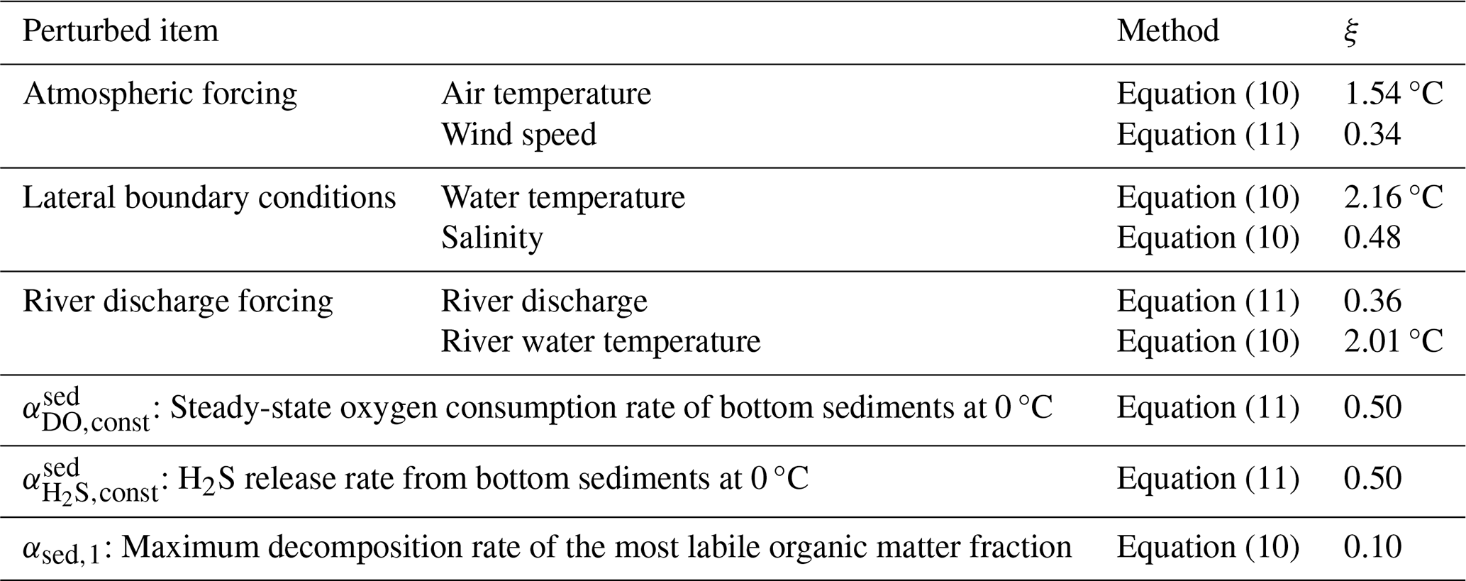
where F_mem indicates the perturbed boundary conditions used for data assimilation, F_base indicates the boundary conditions used for the numerical simulation, and v in Eq. (10) represents an additive perturbation drawn from a normal distribution with a mean of zero and a variance of ξ², having the same units as F. In Eq. (11), v represents a dimensionless multiplicative perturbation drawn from a normal distribution with a mean of zero and a variance of ξ². Equations (10) and (11) were applied according to the type of boundary condition or model parameter involved. The equation selected for each variable is summarized in Table 1.

The model outputs evaluated in this study, as described in Sect. 2.6, were water temperature, salinity, and bottom-layer DO. Accordingly, the application of perturbations was designed to improve the accuracy and practical utility of these three variables. According to a previous study (Matsuzaki and Inoue, 2022), the boundary conditions to be perturbed and the corresponding perturbation magnitudes for temperature and salinity were defined, as shown in Table 1. However, defining appropriate perturbations for DO remains challenging. In this study, perturbations were experimentally applied to three model parameters that exert strong empirical control over bottom-layer DO. The first parameter is ${\mathit{\alpha }}_{\mathrm{DO},\mathrm{const}}^{\mathrm{sed}}$, which represents the steady-state oxygen consumption rate in bottom sediments at 0 °C. The second parameter is ${\mathit{\alpha }}_{{\mathrm{H}}_{\mathrm{2}}\mathrm{S},\mathrm{const}}^{\mathrm{sed}}$, which represents the H₂S release rate from the bottom sediments at 0 °C. The third parameter is α_sed,k, which represents the maximum decomposition rate of the kth fraction.

In this model, a multi-G model that classifies organic matter according to its decomposition rate (Westrich and Berner, 1984) was adopted, with k ranging from 1 to 3. The multi-G model represents organic matter as several fractions with different degradation rates, thereby accounting for the heterogeneous nature of organic matter in sediments. In the present study, perturbations were applied at k=1, which corresponds to the most labile organic matter. The values of ξ are summarized in Table 1. When a small ensemble of random numbers is used to represent a normal distribution, it may deviate substantially from the theoretical normal distribution because of sampling error. Therefore, normally distributed random numbers were not used. Instead, the value assigned to each ensemble member was determined to match the cumulative distribution function of a normal distribution, thereby allowing the distribution to be approximated even with a small ensemble. To avoid unintended correlations among the boundary conditions, the Fisher–Yates shuffle (Fisher and Yates, 1948) was applied for 10 000 shuffle attempts, and the boundary conditions and model parameters were assigned to each ensemble member using the combination that yielded the lowest correlation.

Table 1 Magnitudes of perturbations applied to boundary conditions and model parameters.

2.5 Assimilated observations

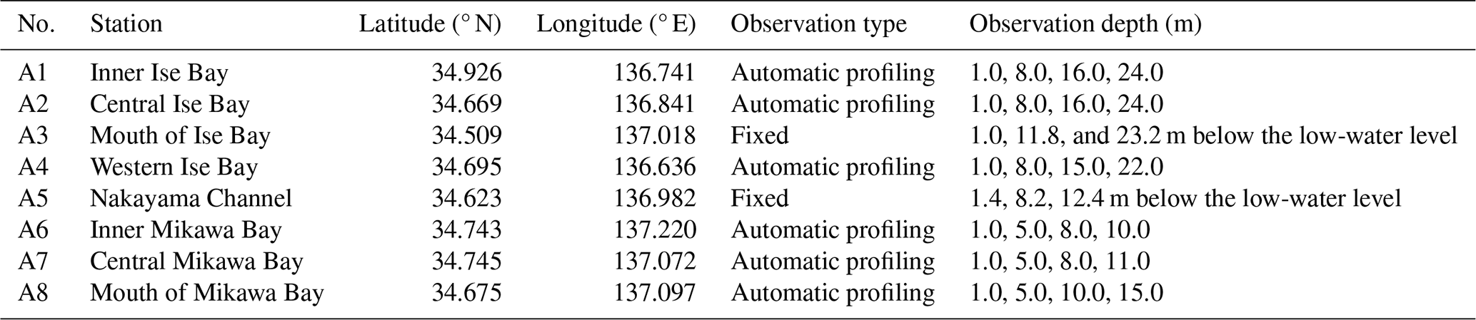
Eight in situ observation stations, listed in Table 2, operate in Ise Bay, and data from these stations were assimilated. The assimilated observations were obtained from monitoring stations operated by the Chubu Regional Development Bureau of the Ministry of Land, Infrastructure, Transport and Tourism. Water temperature, salinity, and DO were measured using CTD instruments. In situ water temperature and salinity profiles, together with in situ bottom-layer DO measurements collected at fixed monitoring stations, were assimilated. The observations were collected at 00:00, 06:00, 12:00, and 18:00 JST without temporal averaging. The observation error variances were set to (1.0 °C)² for water temperature, (1.0)² for salinity, and (1.0 mg L${}^{{}^{-}\mathrm{1}}$)² for DO. The observation error variances for water temperature and salinity were adopted from the previous study by Matsuzaki and Inoue (2022). The specification of the observation error for DO remains a challenging issue in data assimilation studies. Nagano (2025), based on the measurement-based assessment of Irie et al. (2011), adopted 0.59 mg L${}^{{}^{-}\mathrm{1}}$ as a representative effective observation error, with data assimilation performed once per day. In the present study, DO was assimilated every 6 h, which may have increased the influence of short-term variability and spatiotemporal representativeness errors. Accordingly, (1.0 mg L${}^{{}^{-}\mathrm{1}}$)² was adopted as the observation error variance for DO. A gross error check was performed as part of quality control. The difference between the observed and first-guess values was calculated. If this difference exceeded 3 °C for water temperature or 6 for salinity, the corresponding observation was rejected.

Table 2 Assimilated observation data. Observation data from A5 were used for the period from 1 June to 31 December 2022. Observation data from A6, A7, and A8 were used from 20 February 2014 to 31 December 2022 (A6: 11:00 JST, A7: 16:00 JST, and A8: 14:00 JST on 20 February 2014).

A distinguishing feature of this study is the assimilation of continuous in situ observations throughout the water column, including water temperature, salinity, and bottom-layer DO measurements. By incorporating high-frequency observations collected at fixed monitoring stations from the sea surface to the seabed, the dataset provides an improved representation of subsurface physical and biogeochemical variability. This approach helps address limitations associated with reanalysis datasets that rely primarily on satellite-derived observations of the surface.

2.6 Accuracy validation

The model outputs for water temperature, salinity, and DO were compared with in situ profiles of water temperature, salinity, and DO collected at fixed monitoring stations (Table 2). Observation types include vertical profiling via automatic ascent and descent (Automatic profiling), as well as stationary observations (Fixed). Observation data were collected hourly, whereas data assimilation was performed every 6 h; therefore, the comparisons were also conducted at 6 h intervals. The in situ observations used for comparison were collected at 00:00, 06:00, 12:00, and 18:00 JST without temporal averaging. To evaluate the improvement in accuracy achieved through data assimilation, two model output cases were prepared for comparison. Case 1 represents the numerical simulation without data assimilation, whereas Case 2 represents the results obtained after data assimilation.

The accuracy of the model output was assessed using the mean error (ME; Eq. 12), root-mean-square error (RMSE; Eq. 13), correlation coefficient (CC; Eq. 14), standard deviation error (SDE; Eq. 15), and centered (bias-removed) root-mean-square error (CRMSE; Eq. 16):

$$\begin{array}{}\text{(12)}& {\displaystyle }\mathrm{ME}={\displaystyle \frac{\mathrm{1}}{N}}{\sum }_{i=\mathrm{1}}^N\left(m_i-o_i\right)\text{(13)}& {\displaystyle }\mathrm{RMSE}=\sqrt{{\displaystyle \frac{\mathrm{1}}{N}}{\sum }_{i=\mathrm{1}}^N{\left(m_i-o_i\right)}^{\mathrm{2}}}\text{(14)}& {\displaystyle }\mathrm{CC}={\displaystyle \frac{\frac{\mathrm{1}}{N}{\sum }_{i=\mathrm{1}}^N\left(m_i-\stackrel{\mathrm{‾}}{m}\right)\left(o_i-\stackrel{\mathrm{‾}}{o}\right)}{\sqrt{\frac{\mathrm{1}}{N}{\sum }_{i=\mathrm{1}}^N{\left(m_i-\stackrel{\mathrm{‾}}{m}\right)}^{\mathrm{2}}}\sqrt{\frac{\mathrm{1}}{N}{\sum }_{i=\mathrm{1}}^N{\left(o_i-\stackrel{\mathrm{‾}}{o}\right)}^{\mathrm{2}}}}}\text{(15)}& {\displaystyle }\mathrm{SDE}=\sqrt{{\displaystyle \frac{\mathrm{1}}{N}}{\sum }_{i=\mathrm{1}}^N{\left(m_i-\stackrel{\mathrm{‾}}{m}\right)}^{\mathrm{2}}}-\sqrt{{\displaystyle \frac{\mathrm{1}}{N}}{\sum }_{i=\mathrm{1}}^N{\left(o_i-\stackrel{\mathrm{‾}}{o}\right)}^{\mathrm{2}}}\text{(16)}& {\displaystyle }\mathrm{CRMSE}=\sqrt{{\displaystyle \frac{\mathrm{1}}{N}}{\sum }_{i=\mathrm{1}}^N{\left[\left(m_i-\stackrel{\mathrm{‾}}{m}\right)-\left(o_i-\stackrel{\mathrm{‾}}{o}\right)\right]}^{\mathrm{2}}}\end{array}$$

where m_i and o_i are the model outputs and observations, respectively; N is the number of model outputs and observations; and $\stackrel{\mathrm{‾}}{m}$ and $\stackrel{\mathrm{‾}}{o}$ represent the mean values of the model outputs and observations, respectively. The skill scores were calculated for each year, and their mean values over the 12-year study period are presented in Sect. 3.1.

For qualitative validation, representative stations were selected from Stations A1–A8 (Table 2). Time series, scatter plots, and isopleth diagrams are presented for the inner regions of Ise Bay and Mikawa Bay (Stations A1 and A6 in Table 2), where hypoxic conditions are pronounced, and for the mouth of Ise Bay (Station A3 in Table 2), where hypoxia is less severe (Sect. 3.2). We focused on 2021, a year characterized by severe hypoxia, during which an episodic recovery in DO, likely caused by the intrusion of oceanic water, was observed. In addition, the spatial distribution of bottom-layer DO obtained from ship-based observations conducted by the Aichi Fisheries Research Institute was compared with that derived from the data assimilation results (Sect. 3.3). The horizontal distribution maps were generated from spatially sparse observations using the pcolormesh function in Python 3.10.11. Tables and figures for all observation stations (Stations A1–A8; Table 2) are provided in the Supplement.

3 Results

3.1 Overall statistical performance

First, the reproducibility of the physical fields was evaluated. For both water temperature (Fig. 2) and salinity (Fig. 3), data assimilation improved the overall agreement with observations across all stations and depths, although improvements were not observed at every station. When averaged across all stations and depth layers over the 12-year study period, the numerical simulation results for water temperature were substantially improved by data assimilation. The mean error (ME) decreased from 0.95 to 0.31 °C. Similarly, the RMSE decreased from 1.45 to 0.77 °C, the correlation coefficient (CC) increased from 0.98 to 0.99, the standard deviation error (SDE) improved from −0.48 to −0.22 °C, and the centered RMSE (CRMSE) decreased from 0.99 to 0.66 °C.

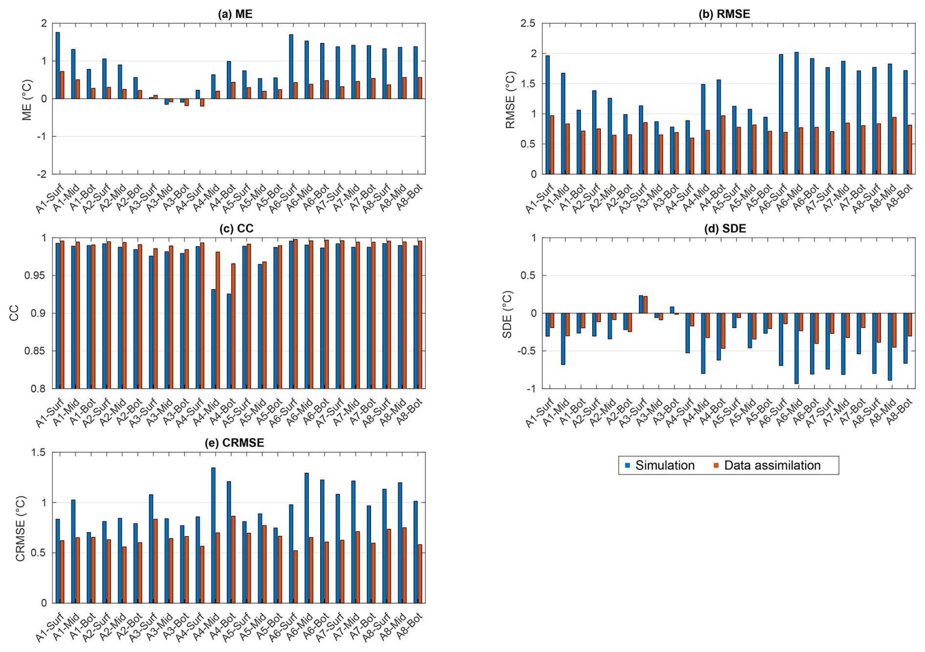
Figure 2 Skill scores for the 12-year numerical simulation and data assimilation results for water temperature at each station (A1–A8) and at each depth layer (surface, middle, and bottom). (a) Mean error (ME), (b) root-mean-square error (RMSE), (c) correlation coefficient (CC), (d) standard deviation error (SDE), and (e) centered root-mean-square error (CRMSE).

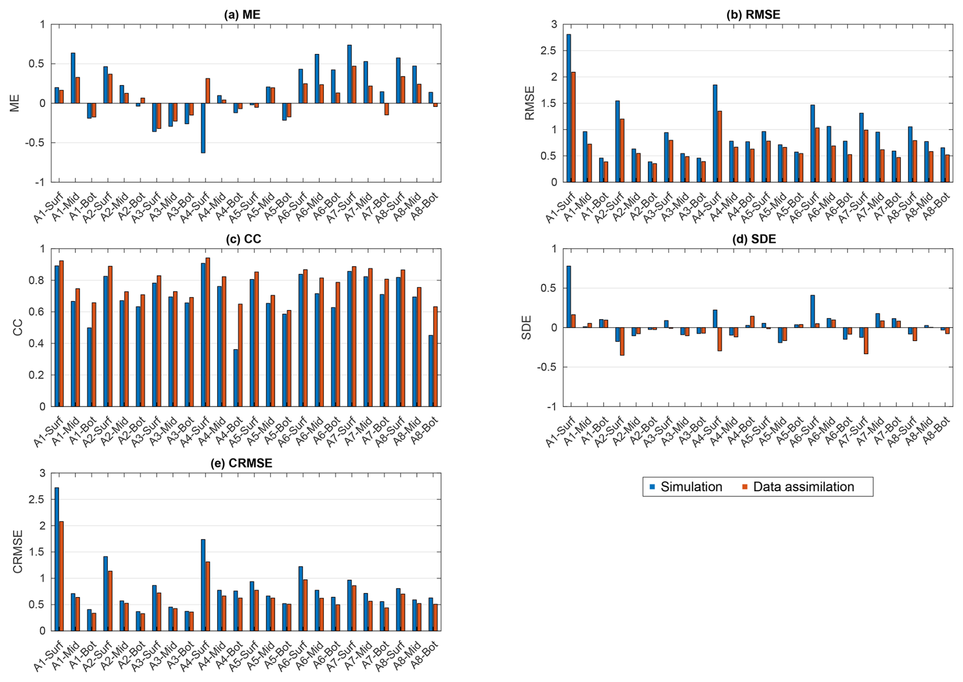
Figure 3 Skill scores for the numerical simulation and data assimilation results for salinity at each station (A1–A8) and depth layer (surface, middle, and bottom). (a) ME, (b) RMSE, (c) CC, (d) SDE, and (e) CRMSE.

Similar improvements were observed in salinity. With data assimilation, the ME decreased from 0.16 to 0.09, the RMSE decreased from 0.96 to 0.74, the CC increased from 0.71 to 0.78, and the CRMSE decreased from 0.84 to 0.70. However, the SDE for salinity was the only metric that did not improve, changing from 0.04 to −0.04.

Next, the reproducibility of DO was assessed (Fig. 4). As with the physical fields, data assimilation improved the overall agreement with observations, although improvements were not observed at all stations. When averaged across all bottom-layer stations over the 12-year study period, the simulated DO values showed improved agreement with observations following data assimilation. The ME decreased from −0.35 to −0.05 mg L⁻¹. Similarly, the RMSE decreased from 1.32 to 1.25 mg L⁻¹, the SDE improved from −0.69 to −0.65 mg L⁻¹, and the CRMSE decreased from 1.12 to 1.01 mg L⁻¹. The CC remained unchanged at 0.85.

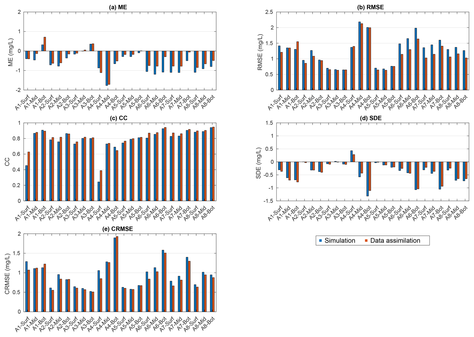
Figure 4 Skill scores for the numerical simulation and data assimilation results for DO at each station (A1–A8) and depth layer (surface, middle, and bottom). (a) ME, (b) RMSE, (c) CC, (d) SDE, and (e) CRMSE. For SI-unit conversion, 1 mg O₂ L⁻¹ = 0.03125 mol m⁻³.

3.2 Temporal and vertical structure variability at representative stations

Representative stations are presented in this section, while complete temporal and vertical validation results for all observation stations and periods are provided in the Supplement. First, we describe the results for the inner region of Mikawa Bay (Station A6), where hypoxic conditions are more pronounced. The seasonal variability in water temperature, as well as the timing of decreases and increases in salinity, was qualitatively consistent across all depth layers (surface, middle, and bottom) (Figs. 5 and 6). The scatter plots of water temperature and salinity indicate that the data assimilation results closely follow the 1:1 line, demonstrating good agreement with the observations.

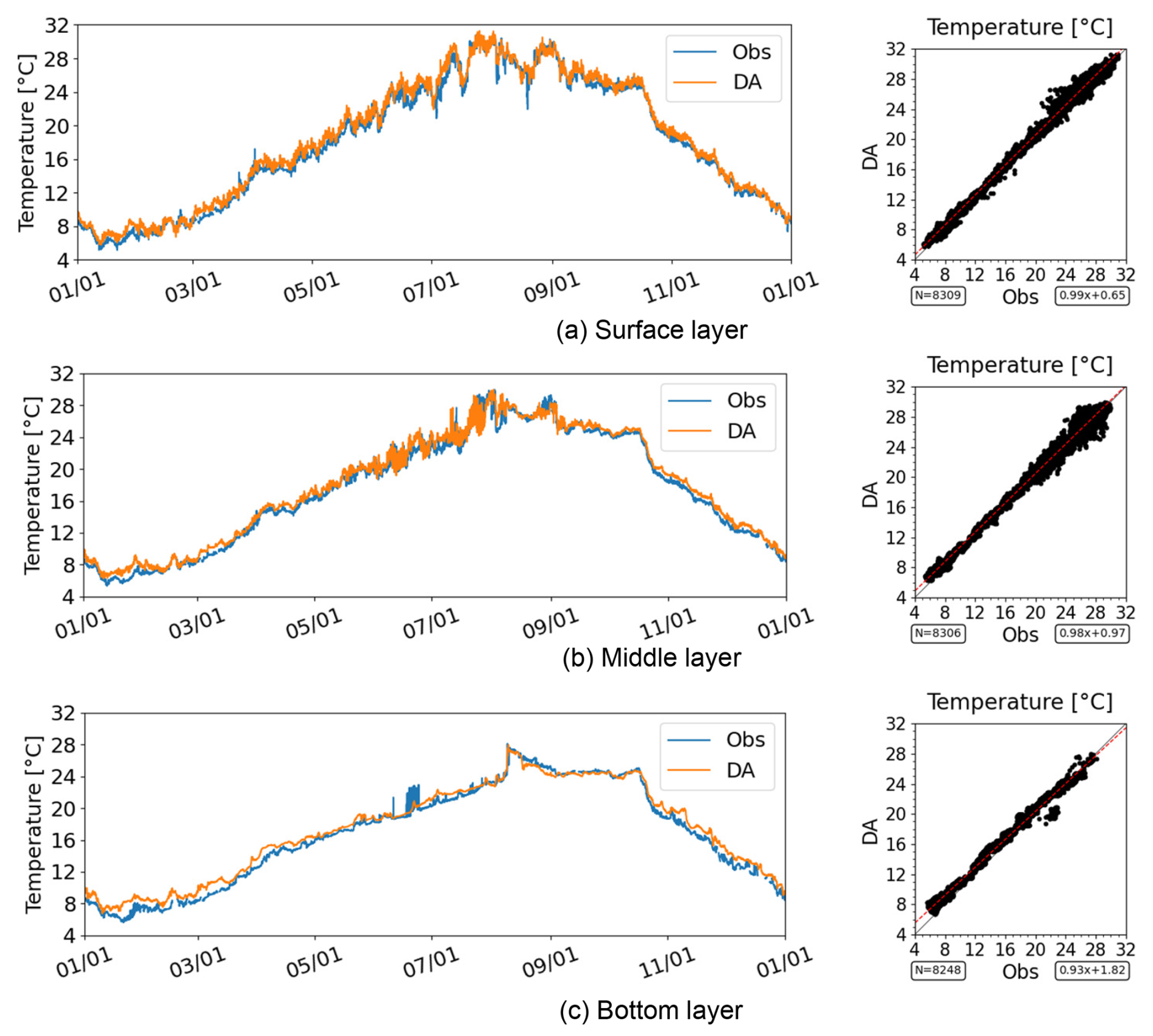
Figure 5 Time series and scatter plots of water temperature in the inner region of Mikawa Bay (Station A6) in 2021.

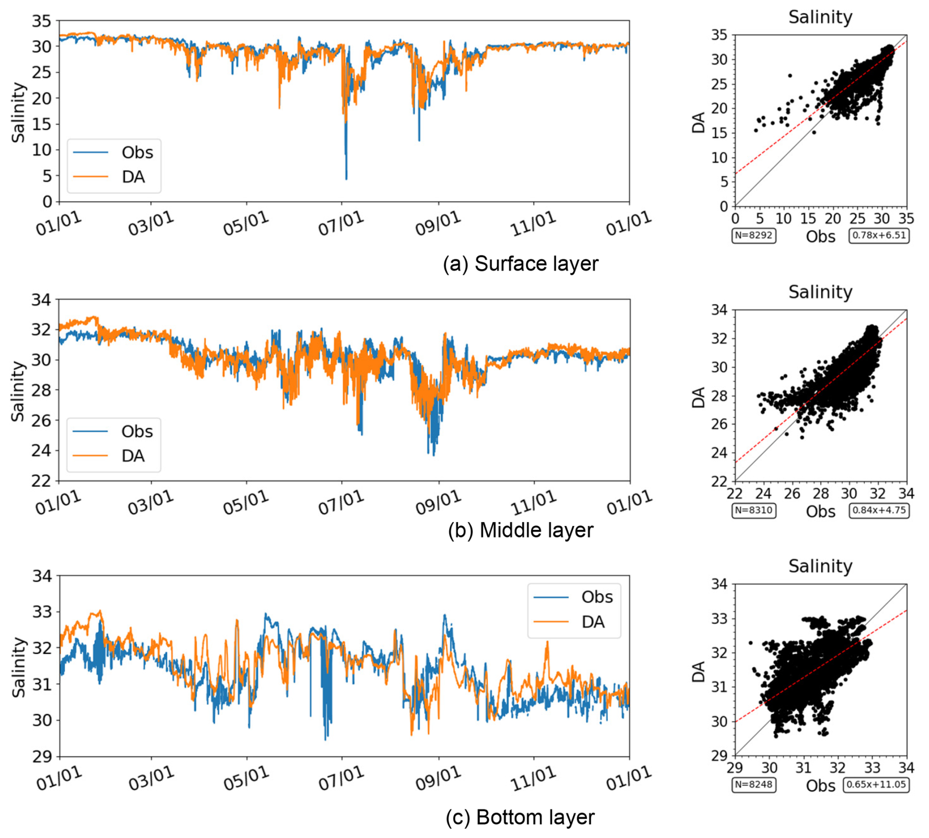
Figure 6 Time series and scatter plots of salinity in the inner region of Mikawa Bay (Station A6) in 2021. Note that the axis ranges differ between panels.

Bottom-layer DO also reproduced the seasonal variability, including the development of hypoxia during summer and its subsequent recovery in autumn (Fig. 7). The timing of the onset and breakdown of stratification was also accurately captured. The scatter plots of DO indicate that the data assimilation results closely follow the 1:1 line, demonstrating good agreement with the observations.

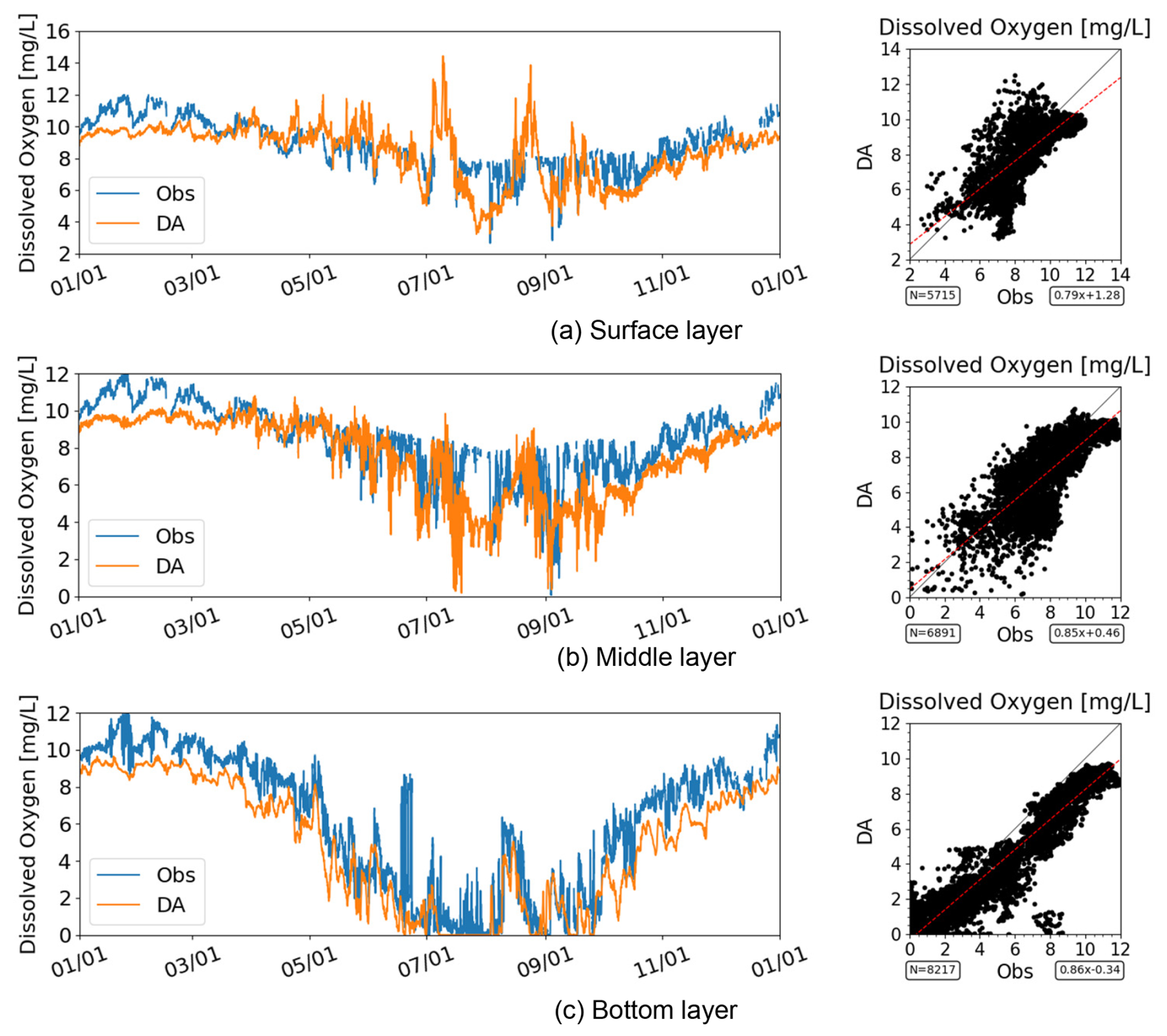
Figure 7 Time series and scatter plots of DO in the inner region of Mikawa Bay (Station A6) in 2021. For SI-unit conversion, 1 mg O₂ L${}^{-\mathrm{1}}=$ 0.03125 mol m⁻³. Note that the axis ranges differ between panels.

The vertical stratification structure (Fig. 8) is well represented, with a strong thermocline developing during summer. Hypoxic conditions developed in the bottom layer during stratified periods, consistent with the observed patterns.

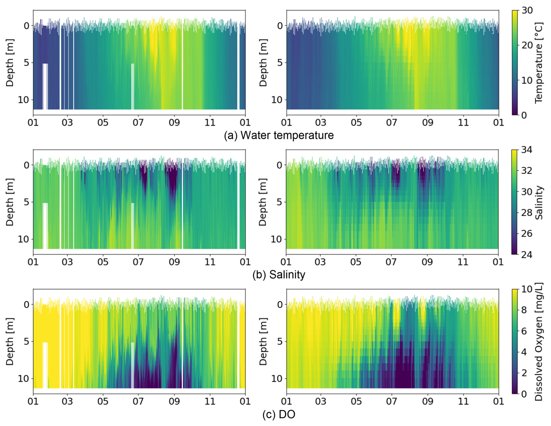
Figure 8 Isopleths of the observed (left) and data-assimilated (right) results in the inner region of Mikawa Bay (Station A6) in 2021. For SI-unit conversion, 1 mg O₂ L${}^{-\mathrm{1}}=$ 0.03125 mol m⁻³.

The data assimilation results successfully reproduced the formation and persistence of hypoxia in the bottom layer.

Next, we examined the inner region of Ise Bay (Station A1), where hypoxic conditions are also observed but are generally less severe than those in the inner region of Mikawa Bay. Seasonal patterns of water temperature and the timing of salinity variations were consistently reproduced across all depth layers (surface, middle, and bottom) (Figs. 9 and 10). The agreement between the data assimilation results and the observations was further supported by the scatter plots, which closely followed the 1:1 line.

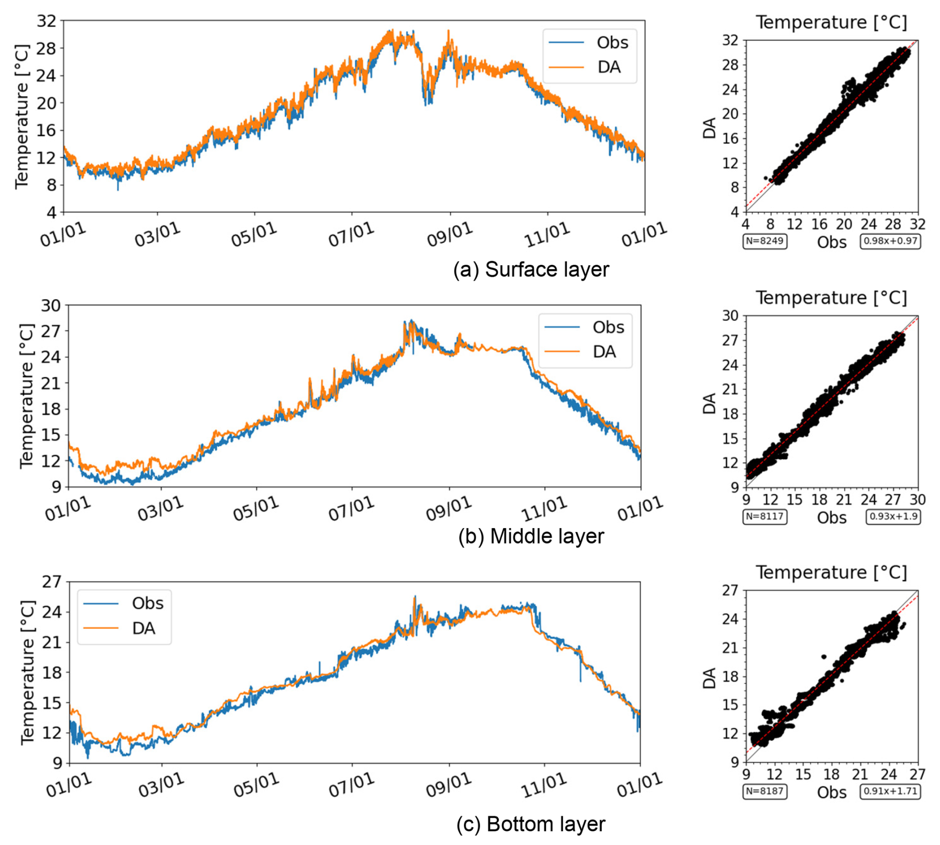
Figure 9 Time series and scatter plot of water temperature in the inner region of Ise Bay (Station A1) in 2021. Note that the axis ranges differ among the panels.

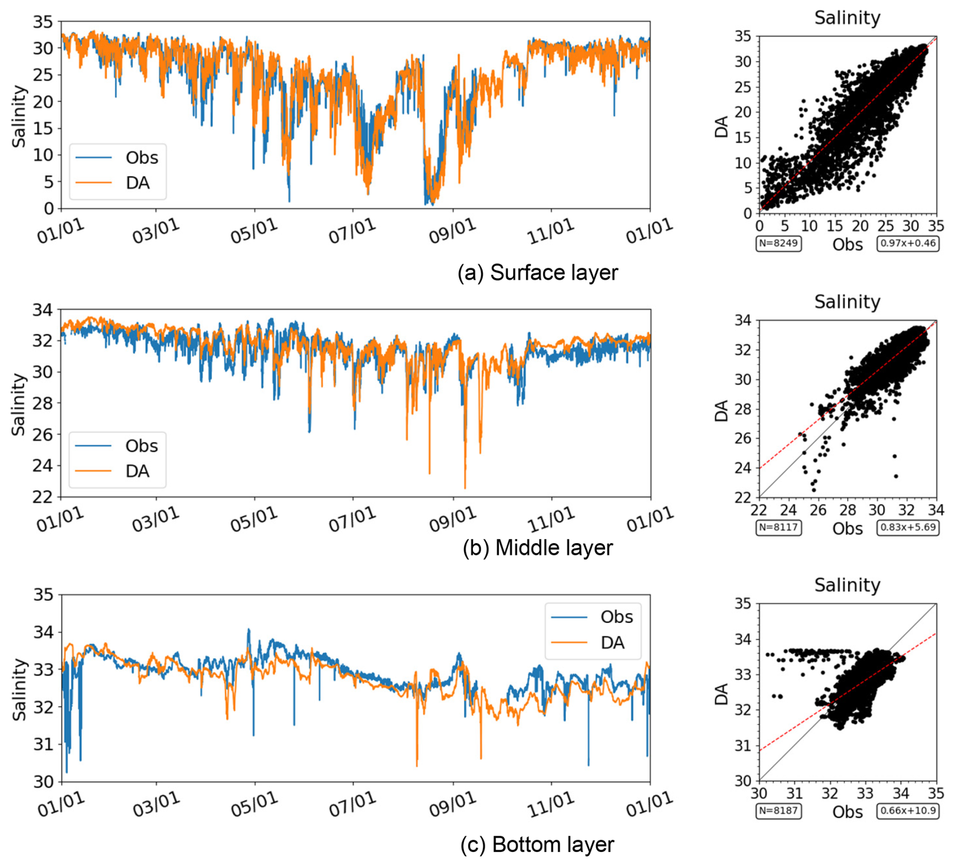
Figure 10 Time series and scatter plot of salinity in the inner region of Ise Bay (Station A1) in 2021. Note that the axis ranges differ among the panels.

Bottom-layer DO also exhibited a similar seasonal cycle, with lower DO concentrations occurring during summer and recovering toward autumn (Fig. 11). The dataset successfully reproduced the seasonal transition from well-oxygenated conditions in winter to hypoxic conditions during summer, followed by recovery in autumn. However, larger deviations from the observations were observed than at the other representative stations. In particular, short-term fluctuations in bottom-layer DO were not always fully reproduced. These results suggest that accurately representing short-term DO variability remains challenging in some areas of the bay. The scatter plots indicate that the data assimilation results are in good agreement with the observed DO concentrations.

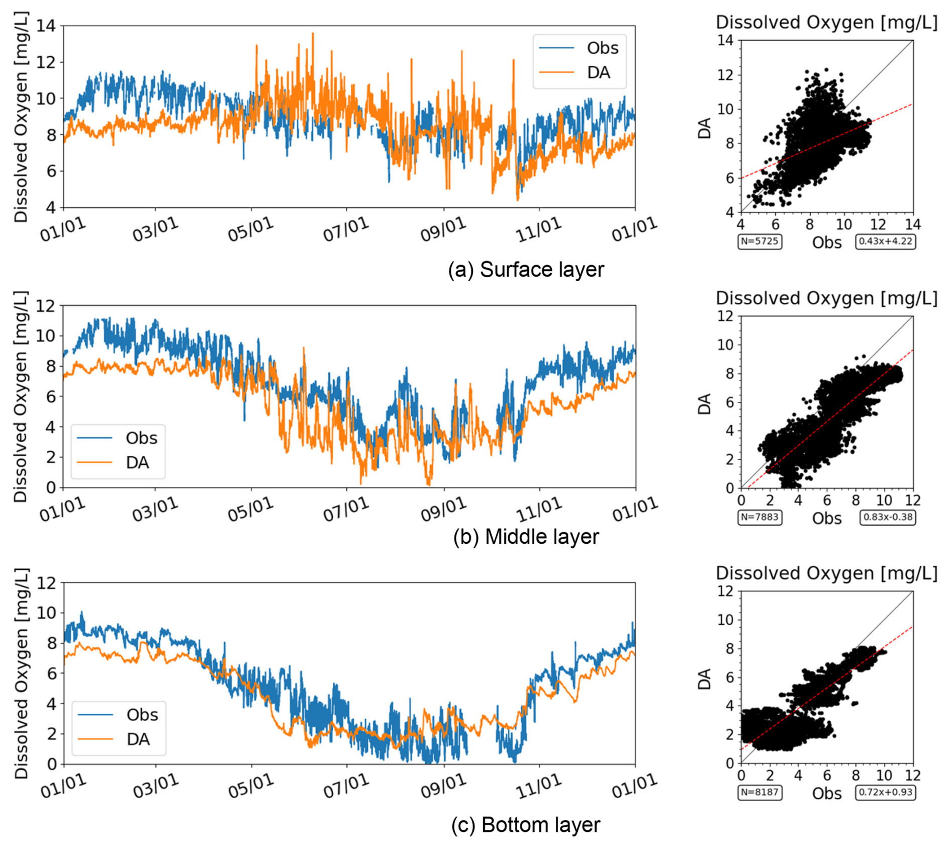
Figure 11 Time series and scatter plot of DO in the inner region of Ise Bay (Station A1) in 2021. For SI-unit conversion, 1 mg O₂ L${}^{-\mathrm{1}}=$ 0.03125 mol m⁻³. Note that the axis ranges differ between panels.

The vertical stratification structure (Fig. 12) was also reproduced, including thermocline formation during summer. Under these stratified conditions, the development of bottom-layer hypoxia was reproduced consistently with the observations. Overall, the data assimilation results provide a consistent representation of the temporal variability and vertical distribution of bottom-layer DO in the inner region of Ise Bay.

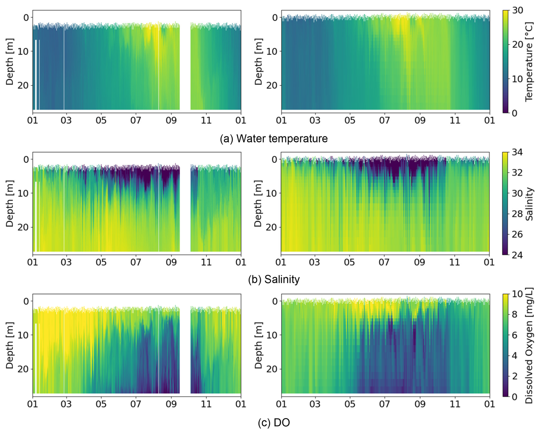
Figure 12 Isopleths of the observed (left) and data-assimilated (right) results in the inner region of Ise Bay (Station A1) in 2021. For SI-unit conversion, 1 mg O₂ L${}^{-\mathrm{1}}=$ 0.03125 mol m⁻³.

Finally, we examined the mouth of Ise Bay (Station A3), where hypoxic conditions were not observed and DO concentrations remained higher than those in the inner regions of the bay. The seasonal variability in water temperature and the timing of salinity changes were consistently reproduced across the surface, middle, and bottom depth layers (Figs. 13 and 14). The scatter plots further demonstrate good agreement between the data assimilation results and the observations, with the data points clustered closely around the 1:1 line.

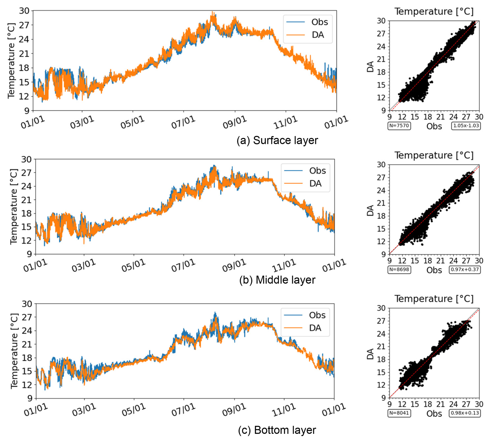
Figure 13 Time series and scatter plot of water temperature at the mouth of Ise Bay (Station A3) in 2021.

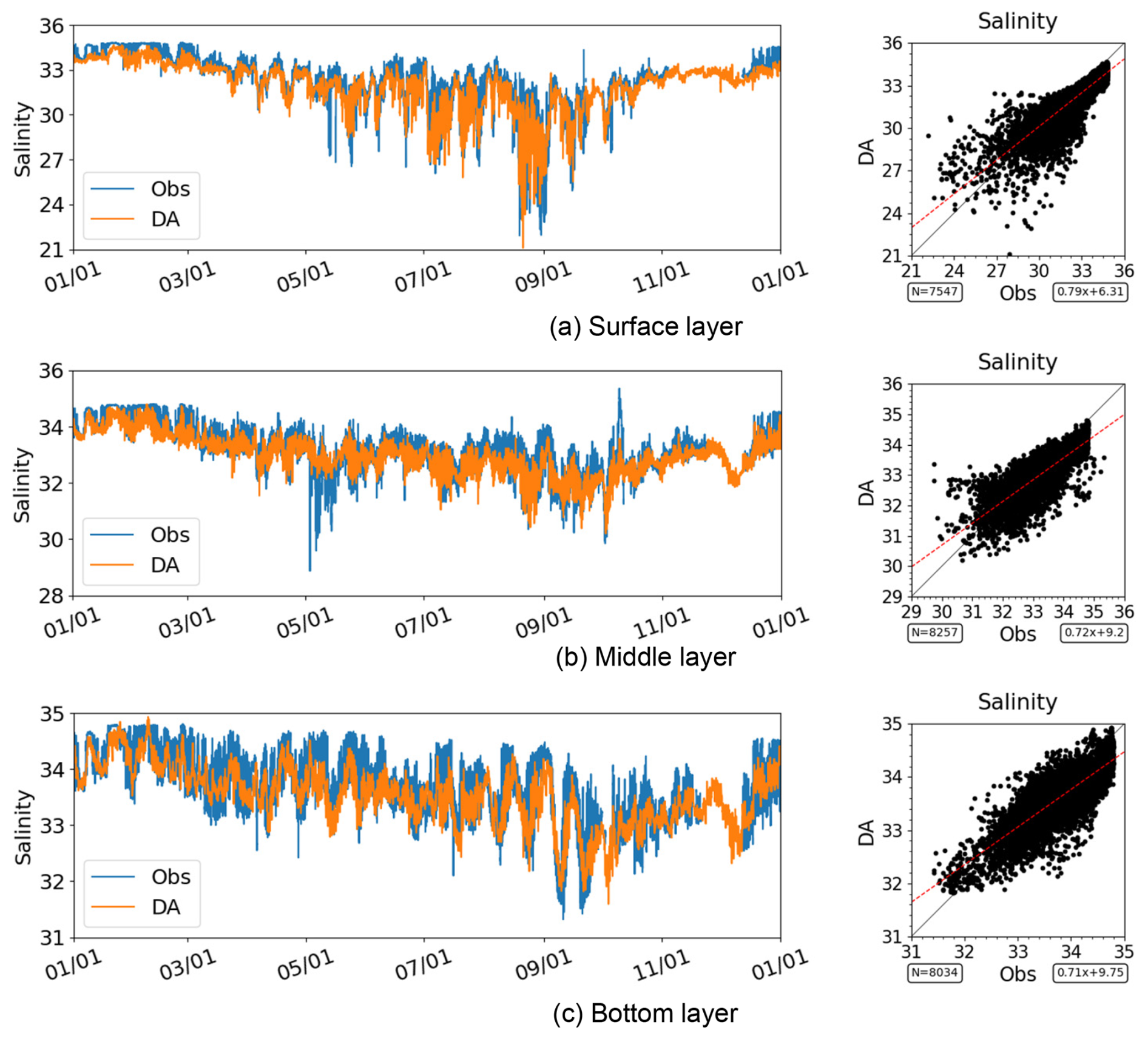
Figure 14 Time series and scatter plot of salinity at the mouth of Ise Bay (Station A3) in 2021. Note that the axis ranges differ among the panels.

Bottom-layer DO also exhibited a distinct seasonal cycle, although its concentrations did not reach hypoxic levels. DO concentrations tended to decrease during summer and recover toward autumn (Fig. 15), and these temporal variations were well reproduced by the data assimilation results. The model captured the transitions between stratified and well-mixed conditions in terms of both timing and overall magnitude. The scatter plots indicate that the data assimilation results are generally consistent with the observed DO concentrations. Overall, the data assimilation results provide a consistent representation of the temporal variability and vertical structure of bottom-layer DO under non-hypoxic conditions at the mouth of the bay.

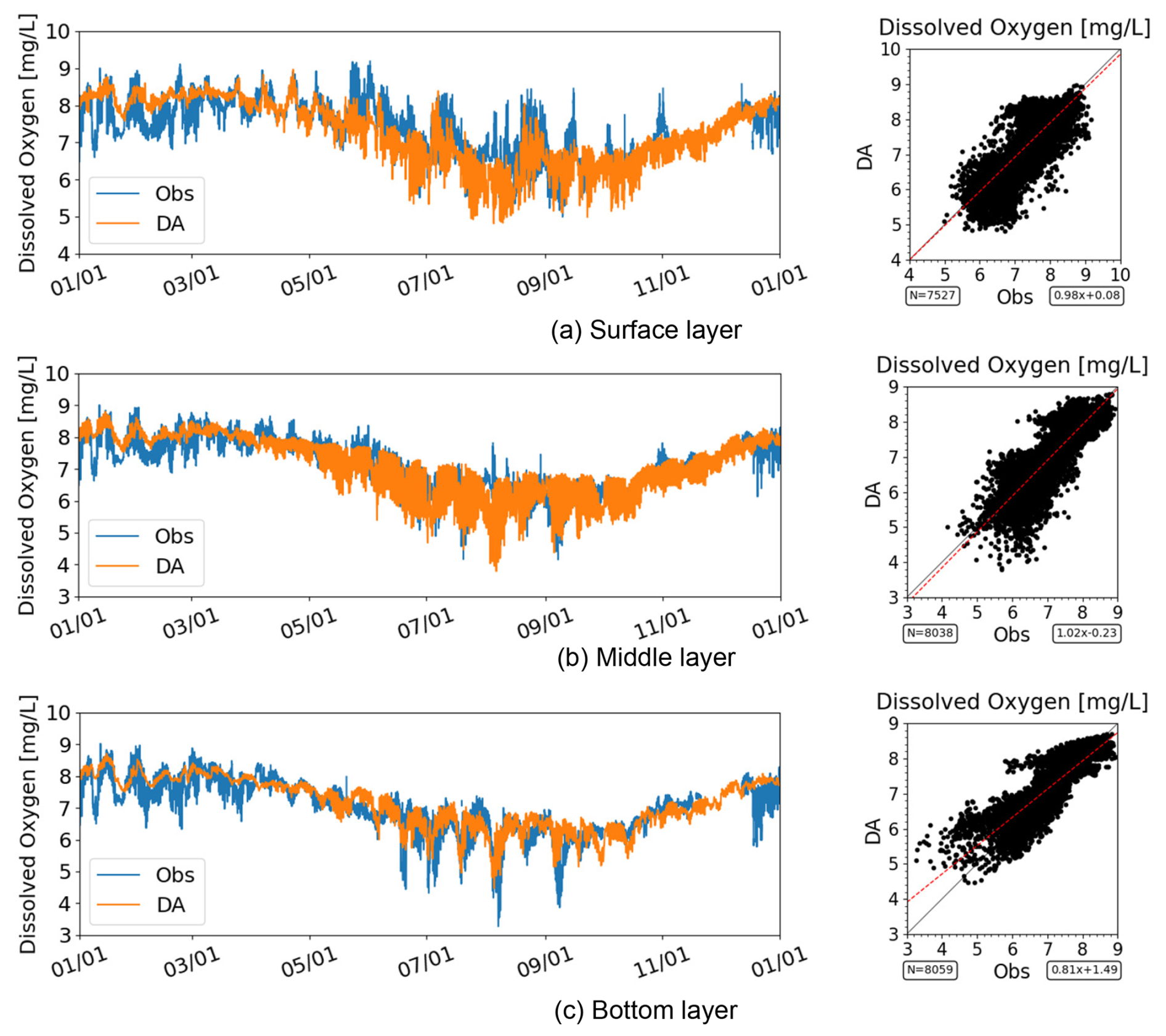
Figure 15 Time series and scatter plot of DO at the mouth of Ise Bay (Station A3) in 2021. For SI-unit conversion, 1 mg O₂ L${}^{-\mathrm{1}}=$ 0.03125 mol m⁻³. Note that the axis ranges differ among the panels.

3.3 Spatial distribution snapshots

Figures 16 and 17 show the horizontal distributions of the observations and data assimilation results for the surface and bottom layers, respectively. Although the observational data were spatially sparse, the data assimilation results reproduced the inflow of high-salinity water from the open ocean and the outflow of low-salinity water along the western coast of Ise Bay. These results are generally consistent with the spatial patterns observed in the observational data.

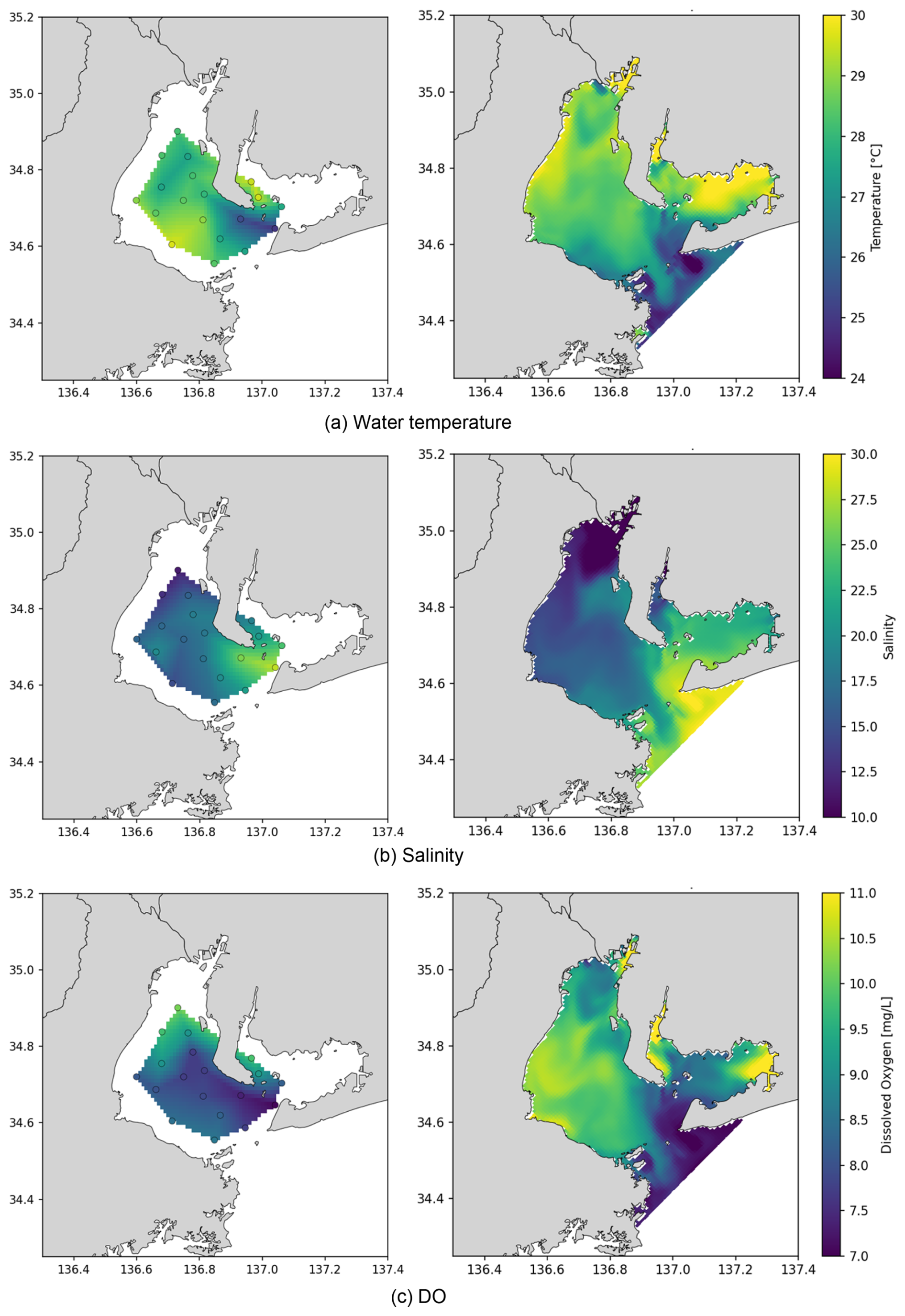
Figure 16 Horizontal distributions of the observed (left) and data-assimilated (right) results in the surface layer at 11:00 on 6 August 2020. (a) Water temperature, (b) salinity, and (c) DO. Circles in the left panels denote the observation locations. For SI-unit conversion, 1 mg O₂ L${}^{-\mathrm{1}}=$ 0.03125 mol m⁻³.

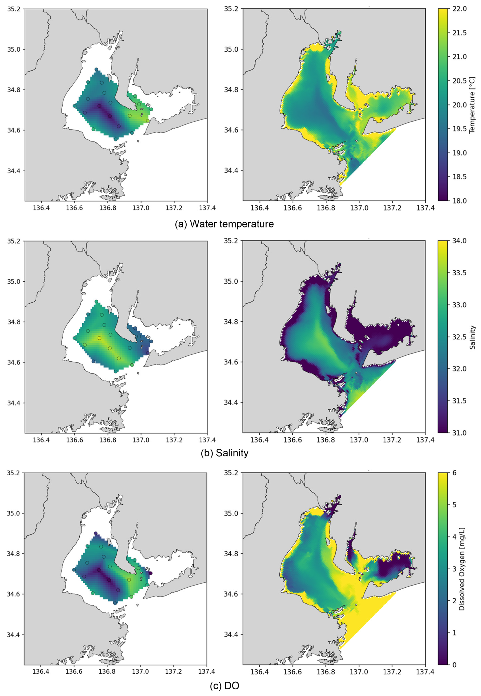
Figure 17 Horizontal distributions of the observed (left) and data-assimilated (right) results in the bottom layer (1.0 m above the seabed) at 11:00 on 6 August 2020. (a) Water temperature, (b) salinity, and (c) DO. Circles in the left panels denote observation locations. For SI-unit conversion, 1 mg O₂ L${}^{-\mathrm{1}}=$ 0.03125 mol m⁻³.

Water temperature and surface DO also exhibited spatial distributions that reflected the influence of both inner-bay and open-ocean water masses, similar to those observed for salinity. In the bottom layer, the data assimilation results indicated an intrusion of high-DO water from the eastern offshore region, resulting in a distinct east–west DO gradient within Ise Bay. A similar spatial pattern was also evident in the observational data. The intrusion of high-DO water masses was further supported by the distributions of bottom-layer temperature and salinity, demonstrating overall consistency between the data assimilation results and the observations. However, some discrepancies remained in the absolute DO concentrations. For example, at 11:00 on August 6, the data assimilation results slightly underestimated DO concentrations relative to the observations. These results indicate that the data assimilation framework effectively reconstructs mesoscale spatial structures in both physical and biogeochemical fields despite the limited availability of observational data.

4 Discussion

The IBRA dataset was developed in this study to provide a reanalysis dataset with three key features. First, unlike many previous reanalysis datasets that rely primarily on satellite observations, IBRA assimilates continuous in situ measurements throughout the water column, including high-frequency DO observations, thereby improving the representation of subsurface variability. Second, the 6 h assimilation cycle enables the dataset to resolve short-term variability driven by tidal processes, which are a dominant control of coastal transport and mixing. Third, spatially coherent corrections are applied across the entire bay using an EnKF, ensuring spatial consistency in both physical and biogeochemical fields while avoiding artificial discontinuities often associated with simpler data assimilation approaches. Based on the results presented in Sect. 3, the extent to which these objectives were met is discussed below.

4.1 Assimilation of subsurface observations

The statistical metrics for water temperature, salinity, and DO show improvements across the entire bay (Figs. 2–4), indicating that the assimilation of water-column observations is effective. By incorporating continuous in situ measurements throughout the water column, IBRA provides a more realistic representation of subsurface physical and biogeochemical variability.

4.2 High-frequency data assimilation

In this study, the performance of the 12-year reanalysis dataset was evaluated primarily in terms of long-term accuracy rather than its ability to represent short-term variability. Previous work (Mizuguchi et al., 2025) demonstrated that assimilating observations at 6 h intervals effectively improves the representation of physical fields in coastal environments influenced by tidal currents.

Consistent with this finding, the CC for salinity improved from 0.71 to 0.78 in the present study (Fig. 3), suggesting that the data assimilation framework contributes to a better representation of temporal variability. Therefore, the present dataset, which adopts a similar high-frequency data assimilation strategy, is expected to provide an improved representation of short-term variability. The ability to capture rapid changes associated with stratification, mixing, and water mass exchange can be partly attributed to the 6 h data assimilation cycle. However, a more detailed evaluation of short-term processes remains an important subject for future study.

4.3 Spatial consistency

Based on the one-year isopleth diagrams presented in Sect. 3.2 (Figs. 8 and 12) and the horizontal distribution snapshots presented in Sect. 3.3 (Figs. 16 and 17), no artificial discontinuities or unrealistic density inversions in salinity or temperature were observed. This finding is further supported by the Supplement, which provide isopleth diagrams for all stations throughout the 12-year study period. These results suggest that the data assimilation framework provides spatially consistent corrections across the entire bay, thereby avoiding localized or discontinuous adjustments that are often associated with simpler data assimilation approaches. Although the effect of applying spatially coherent corrections across the entire domain cannot be quantified rigorously, the results qualitatively suggest that this approach is effective.

5 Data description and access

5.1 Dataset overview

The IBRA dataset provides a 12-year (2011–2022) high-resolution reanalysis of ocean circulation and biogeochemical variables in Ise Bay, Japan. The dataset is based on a coupled ocean circulation–ecosystem model and a data assimilation system incorporating in situ observations of water temperature, salinity, and DO. The dataset has an hourly temporal resolution and resolves the full water column using 38 vertical layers across a horizontal grid of 85 × 85 cells. All timestamps are reported in Japan Standard Time (JST; UTC+9). Data assimilation is performed every 6 h (00:00, 06:00, 12:00, and 18:00 JST); these time points correspond to the analysis states, whereas the intermediate hourly data represent forward simulations initialized from the preceding analysis state. This temporal structure allows the dataset to represent both short-term variability, including tidal processes, and longer-term seasonal variability. In particular, the inclusion of bottom-layer DO observations enables a detailed assessment of hypoxic conditions in enclosed coastal waters.

5.2 Variables and file structure

The dataset includes three primary variables: water temperature (°C), salinity, and DO (mol m⁻³), available at all grid points and vertical layers. In the distributed dataset, DO is reported in units of mol m⁻³, whereas mg L⁻¹ is used in the figures and statistical analyses presented in this manuscript for consistency with common practice in coastal environmental engineering. In addition to these variables, the dataset includes water level (m) and horizontal velocity components in the x- and y-directions (m s⁻¹). These variables were generated using the coupled hydrodynamic–ecosystem model and data assimilation system described in Sect. 2. Although these variables were not evaluated in this study, they are provided to support potential users. The data are distributed in NetCDF4 format and organized into annual files, with one file provided for each year. Each file contains multidimensional arrays with dimensions corresponding to time, horizontal coordinates, and vertical layers. Standard metadata, including variable definitions, physical units, and coordinate systems, are provided in accordance with common oceanographic data conventions to facilitate data interoperability and reuse.

5.3 Usage notes and limitations

The IBRA dataset is designed to provide a more accurate representation of subsurface physical and biogeochemical processes, particularly bottom-layer DO variability. However, this study has several limitations. The accuracy of the dataset may vary depending on the location and environmental conditions. In particular, discrepancies persist in the absolute DO values during periods of rapid variability, such as intense mixing events. Therefore, users should consider these uncertainties when applying the dataset to quantitative analyses and assessments. Despite these limitations, the dataset provides a robust and dynamically consistent representation of physical and biogeochemical conditions within an enclosed coastal system. It is expected to serve as a valuable resource for scientific research and environmental assessment.

6 Data availability

The IBRA dataset is publicly available via Zenodo at https://doi.org/10.5281/zenodo.19808667 (Matsuzaki et al., 2026). The dataset is distributed as annual NetCDF files covering the period 2011–2022. Detailed instructions for downloading and using the data, including file descriptions and metadata, are available in the repository. The dataset is distributed under the Creative Commons Attribution 4.0 International (CC BY 4.0) License.

7 Conclusions

The IBRA dataset provides a high-resolution, long-term reanalysis of coastal circulation and biogeochemical conditions within a semi-enclosed coastal environment. With hourly temporal resolution, full water-column coverage, and assimilation of in situ observations, the dataset is well suited to a wide range of scientific and practical applications. Key features include spatially consistent corrections across the bay, high-frequency data assimilation capable of resolving tidal-scale variability, and the incorporation of continuous water-column observations, including DO, thereby enabling improved representation of subsurface processes. One of the primary applications of IBRA is the assessment of hypoxic conditions in semi-enclosed coastal waters. The dataset enables detailed analyses of the temporal evolution, spatial distribution, and interannual variability of bottom-layer DO, thereby providing insights into the mechanisms underlying hypoxia formation and dissipation. IBRA can also support evaluations of compliance with environmental quality standards based on bottom-layer DO concentrations, which are increasingly being implemented in Japan. In addition, the dataset can be used to investigate physical–biogeochemical interactions in coastal environments, including the effects of stratification, tidal forcing, and water-mass exchange between the open ocean and inner-bay regions. The high temporal resolution and frequent data assimilation allow the dataset to capture short-term variability, including episodic mixing events and rapid changes in DO associated with oceanic intrusions. The IBRA dataset is also valuable for model validation and data-driven analyses and can provide boundary or initial conditions for regional and local modeling studies. Furthermore, it may serve as a valuable resource for stakeholders involved in coastal management, environmental planning, and ecosystem assessment. Despite these advantages, several limitations remain. Although the dataset reproduces the overall variability and spatial structure of the physical and biogeochemical fields, discrepancies persist in absolute DO values under certain conditions, particularly during periods of rapid variability that cannot be fully resolved by the circulation model. These uncertainties should be considered when applying the dataset in quantitative analyses. In summary, IBRA provides a comprehensive and dynamically consistent representation of the physical and biogeochemical conditions in Ise Bay. By combining high-resolution modeling with in situ data assimilation, the dataset addresses an important gap in coastal reanalysis products and is expected to contribute to both scientific research and environmental management.