HUST-Grace2026s: a high-resolution static gravity field product from GRACE and GRACE-FO observations (2002–2025)

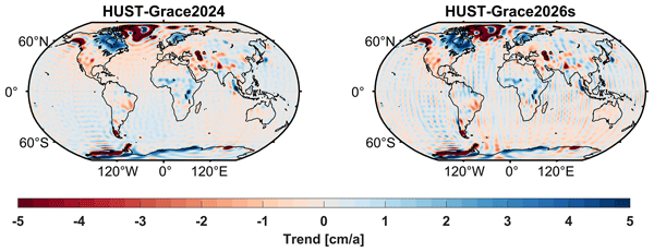
HUST-Grace2026s is a GRACE-only static gravity field determined by HUST (Huazhong University of Science and Technology). It's determined based on more than 20 years' observation data from GRACE (Gravity Recovery and Climate Experiment) and its successor GRACE-FO. The model provides high spatial resolution (up to degree/order 180) for mass distribution monitoring, complementing temporal series like HUST-Grace2024.

This study presents the motivation and key outcomes behind our new static gravity field model, HUST-Grace2026s: (1) Merely adding current GRACE-FO observations offers limited improvement to existing GRACE-only models, due to GRACE-FO's current orbital altitude. (2) The application of stochastic model based on postfit residual significantly enhances accuracy, reducing cumulative geoid error by up to 66 % at degree 180 compared to the nominal strategy. (3) The benefit of LRI data on static gravity field determination is strongly tied to the strategy for estimating rate terms. (4) Comprehensive internal and external validation confirms that HUST-Grace2026s achieves higher spatial resolution than unregularized solutions and improves accuracy by over 50 % compared to its predecessor, HUST-Grace2016s. This product serves as a benchmark for long-term mass change studies.

The primary model data consisting of potential coefficients representing Earth's static gravity field, together with secular and annual variations. This data set is identified with the following DOI: https://doi.org/10.5880/icgem.2026.001 (Zhou et al., 2026b).

1 Introduction

The Gravity Recovery and Climate Experiment (GRACE) gravity mission, which has been developed by National Aeronautics and Space Administration (NASA) and the German Aerospace research and technology Center (DLR) in 2002, offered us a new insight of monitoring the mass transportation on earth at the accuracy of 1 cm Equivalent Water Height (Tapley et al., 2004). The GRACE mission was equipped with accurate GNSS receivers for measuring the orbital position of both satellites with the precision of a few centimetres and a K/Ka-band MicroWave Instrument (MWI) ranging system for monitoring the intersatellite distance with a high accuracy of µm s⁻¹ and SuperSTAR sensors for observing the non-gravitational force acted on the satellites (Flury et al., 2008). Based on the observation data provided by the GRACE mission, researchers have developed a series of the monthly gravity field products and the mean gravity field products (Chen et al., 2018, 2019; CSR, 2024; Dahle et al., 2019; JPL, 2024; Kvas et al., 2019; Zhou et al., 2017; Zhou et al., 2024).

Benefit from the tremendous success of the GRACE mission, its successor GRACE-FO was launched in 2018, which has been on stage for more than 6 years up to now. GRACE-FO is equipped with two kinds of ranging systems consisting of laser ranging interferometer (LRI) and MWI (Landerer et al., 2020). The LRI ranging system has lower systematic noise than that in MWI, ensuring the high accuracy of recovering the temporal gravity field (Abich et al., 2019; Wegener et al., 2020). Therefore, many researchers focus on the potential of LRI in temporal gravity field determination, especially on the aspect of the ability to gain the hydrology signal compared with MWI. Pie et al. (2021) performed the temporal gravity field recovery based on the range-rate data derived from both LRI and MWI, and the result indicated LRI has a similar performance in the context of gaining temporal gravity signal compared with that of MWI. In order to make full use of the higher accuracy of LRI, Han et al. (2021) applied the line-of-sight gravity difference (LGD) approach based on LRI data and used it to detect the extreme weather processes like floods. Ghobadi-Far et al. (2022) also used the LGD approach based on the LRI data to monitor the hydrological process on land. In short, the previous LRI-related researches mainly focus on the applications in short time period like a few days, monthly. These researches lack of the application of LRI in long time period such as yearly or even longer. These works inform our integration of LRI data into the static gravity field. Ghobadi-Far and McCullough (2024) used the one-year LRI data to validate the state-of-the-art global static gravity field including GGM05C (Ries et al., 2016), ITSG-Grace2018s (Kvas et al., 2019), GOCO-TIM-R06e (Zingerle et al., 2019), EIGEN-6C4 (Förste et al., 2014), and GOCO06s (Kvas et al., 2021). However, the research only focusses on the validation of the performance of the previous global static gravity field, not the determination of static gravity field itself. Therefore, it is valuable to do some researches on the contribution of LRI or even the GRACE-FO data in static gravity field determination.

It's of great importance to validate the performance of LRI observation data during the mean field recovery compared with that based on MWI. As one of the crucial input data during gravity field determination, the quantity of level-1B LRI data will play a vital role in the processing chain. Apart from the official LRI1B products provided by the NASA Jet Propulsion Laboratory (JPL), there are several kinds of alternative in-house LRI1B data developed by different analytical centres, including the Albert Einstein Institute (AEI), Sun Yat-sen University (SYSU) and HUST. Level 1A LRI data preprocessing involves addressing issues like phase jump removal using published techniques (Müller et al., 2022; Misfeldt et al., 2023; Müller et al., 2024), ensuring high-quality input for the gravity field product. Öhlinger et al. (2025a) determined the preliminary static gravity field GOCO25 up to degree and order 250 based on both MWI data and LRI data derived from AEI and published the final products GOCO2025s (Öhlinger et al., 2025b). The preliminary result GOCO25 has shown that LRI data can significantly improve the accuracy of zonal coefficients. However, the LRI1B data product derived from the only analytics centres can't obtain an optimal static gravity field, and it's reasonable to combine different LRI1B data products to minimize the noise, achieving the optimal mean gravity field determination (Meyer et al., 2019). That is one of the motivations of the study, in short, enabling a quantitative analysis for the contribution of LRI data during the static gravity field determination.

A further motivation for this work is to determine a consistent static gravity field for the GRACE era that also incorporates data from the GRACE-FO mission, thereby providing a unified model for characterizing Earth's mass distribution across both satellite generations. Static global gravity fields serve as critical infrastructure for a wide range of scientific and engineering applications, including geoid determination, satellite orbit prediction, navigation, and resource exploration. Numerous satellite-only mean gravity field models have been produced from dedicated gravity missions such as CHAMP, GRACE, and GOCE. These include GRACE-only models (e.g., HUST-Grace2016s, Tongji-Grace02s, ITSG-Grace2018s, AIUB-GRACE03s), GOCE-only models (GOSG02S, GO_CONS_GCF_2_TIM_R6), and combined solutions (e.g., GOCO06s, GOCO2025s). However, a common limitation among these existing products is that none of them include observations from the GRACE-FO mission. This omission creates a gap in creation of a seamless, long-term static gravity field product that bridges the GRACE and GRACE-FO data records. The GRACE-FO mission has now accumulated approximately six years of scientific data, which have been extensively used to monitor time-variable processes such as terrestrial water storage changes (Zhao et al., 2025; Romero and Piña, 2025; Zhao et al., 2024; Zhou et al., 2026a; Zhou et al., 2025), extreme hydrological events (Li et al., 2024a; Wu et al., 2025; Ma et al., 2024; Xie et al., 2022), and glacier mass balance (Shi et al., 2024; Jenny et al., 2025; Li et al., 2022), primarily through monthly solutions or along-track data with spatial resolutions of several hundred kilometres. While these applications leverage the high temporal resolution of the data, the static gravity field offers complementary value by providing higher spatial resolution (e.g., ∼100 km), albeit at the cost of temporal resolution. This high-resolution static field is crucial for applications including lithospheric density modelling (Braitenberg et al., 2025; Buoninfante et al., 2023), local geoid determination (Natsiopoulos et al., 2023), and establishing a baseline for long-term mass change studies. Therefore, a critical and unresolved task of this study is to quantitatively assess the contribution of GRACE-FO observations to static field determination and to generate a unified, consistent static gravity field model that seamlessly bridges the GRACE and GRACE-FO eras. In all, our model HUST-Grace2026s mainly focus on the construction of baseline for the long-time mass change variation research, bridging the gap of GRACE and GRACE-FO observation period, which is different from the current established static gravity field models.

This paper is described as follow: Section 2 details our processing chain during the determination of HUST-Grace2026s. Section 3 depicts the contribution of LRI data based on different parameter estimation strategies and evaluate the performance of HUST-Grace2026s comparing with other GRACE-only static gravity field though both internal and external validations. Section 4 is for conclusion.

2 Methods and data processing

2.1 Background models and GRACE/GRACE-FO data

The gravity field model determination is a parameter estimation problem, which can be resolved by Least Square (LS) approach. According to the different kinds of hypothesis, the LS Approach can be further achieved based on functional models such as dynamic approach, short-arc approach, energy-balanced approach and so on. The dynamic approach has been widely used by different GRACE data analysis centres around the world including Center for Space Research (CSR), German Research Centre for Geosciences (GFZ), Jet Propulsion Laboratory (JPL), Huazhong University of Science and Technology (HUST) and so on. We utilize an in-house gravity field determination software based on the dynamic approach and publish several kinds of GRACE-only temporal or static gravity field products including HUST-Grace2016s, HUST-Grace2020 and HUST-Grace2024 (Zhou et al., 2017, 2019, 2024). During our latest static gravity field product HUST-Grace2026s determination (background model details as shown in Table 1), the background models are basically the same as the models used in the determination of HUST-Grace2024 except for several aspects as follow:

Table 1 Summary of force models and estimated parameters during the HUST-Grace2026s static gravity field determination.

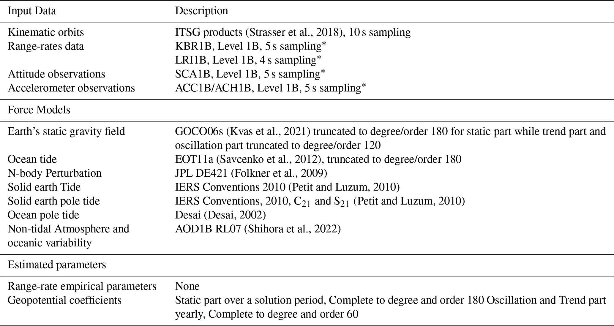
^∗ The HUST-Grace2026s static field incorporates a continuous 23-year dataset from April 2002 to March 2025, seamlessly combining GRACE and GRACE-FO observations. The input data include: GRACE KBR/SCA Release 03 (April 2002–June 2017) with accelerometer data transitioning from RL02 to RL03 in November 2016 to maintain data continuity; and GRACE-FO Level-1B Release 04 products (June 2018–March 2025) enhanced by LRI data from January 2019. This integrated dataset provides the temporal coverage and consistency required for high-precision static gravity field determination.

Firstly, we have used the latest LRI1B dataset including AEI-V54 LRI1B (Müller, 2021; Yan et al., 2021), JPL RL04 LRI1B (Wen et al., 2019), SYSU-V10 LRI1B (Yin et al., 2024) and HUST-V01 LRI1B (Li et al., 2025). The LRI1B data used in our manuscript is performed by the CRN filter (a kind of low pass anti-aliasing filter) and the filter properties are the same. So, we don't perform any other low-pass filter before down-sampling the LRI1B data to 4 s (original data in 2 s) and we think the impact of this strategy is minor. Secondly, we apply a stochastic model based on autocorrelation coefficients which are derived from postfit residual, following the established approaches (i.e. Guo et al., 2018; Chen et al., 2019). The post-fit residual is derived during the temporal gravity field determination, in other words, less post-fit residual is observed, and the accuracy of temporal gravity field is better. Therefore, it's reasonable that the stochastic model is determined based on post-fit residual in our manuscript. More details about the stochastic model will be described in Sect. 2.2.

Lastly, beyond the static parameter determination, we also estimate the oscillation and trend parameters to degree and order 60. Besides, we need to address about this: both the trend/oscillation parameters and the static parameters are estimated simultaneously as independent parameters. In other words, the static/temporal parameters from our final solution are different from the background model. As for the truncation degree of trend/oscillation parameters, we also design an experiment using GOCO06s (See Fig. S1 in the Supplement). The experiment is designed as we allowed its time-variable coefficients to evolve with time and then superimposed them onto the static coefficients and calculate the geoid height difference between the base model EIGEN-6C4 and the new geopotential coefficients derived from GOCO06s. The result indicate that the variation of geoid height difference curves mainly is up to degree 60, while the higher degrees remain unchanged. This demonstrates that the temporal signals have negligible power beyond approximately degree 60. The lower truncation degree for temporal parameters do help to accelerate the calculation process under our in-house gravity field determination software. However, it should keep in mind that the different truncation degree for static/temporal parameters is a kind of implicit regularization for the static parameters beyond degree 60. More details about the effect of trend/oscillation parameters estimation during the static gravity field determination will also be described in Sects. 2.3 and 3.1.

The gravity field determination mainly starts from the Eq. (1):

$$\begin{array}{}\text{(1)}& \begin{array}{rl}\mathrm{\Delta }V& (r,\mathit{\phi },\mathit{\lambda })={\displaystyle \frac{\text{GM}}{R}}\sum _{l=\mathrm{0}}^{N_{max}}\sum _{m=\mathrm{0}}^l{\left({\displaystyle \frac{R}{r}}\right)}^{l+\mathrm{1}}\\ & \times \left(\mathrm{\Delta }{\stackrel{\mathrm{‾}}{C}}_{lm}\cos \right(m\mathit{\lambda })+\mathrm{\Delta }{\stackrel{\mathrm{‾}}{S}}_{lm}\sin (m\mathit{\lambda }\left)\right){\stackrel{\mathrm{‾}}{P}}_{lm}\left(\sin \mathit{\phi }\right)\end{array}\end{array}$$

where GM, R, r denotes as the constant value for earth, the mean radius of earth and height over the earth surface, in this article, mainly refer to the orbital altitude of GRACE/GRACE-FO satellite. And N_max, m, l are the maximum truncated order for gravity field model, the order of normalized geopotential coefficients, the degree of normalized geopotential coefficients respectively. And $\mathrm{\Delta }{\stackrel{\mathrm{‾}}{C}}_{lm}$, $\mathrm{\Delta }{\stackrel{\mathrm{‾}}{S}}_{lm}$ are the variation of normalized geopotential coefficients with respect to the background gravity field model, ${\stackrel{\mathrm{‾}}{P}}_{lm}\left(\sin \mathit{\phi }\right)$ is the normalized Legendre coefficients.

In the Eq. (1), we can easily find a term named $(\frac{R}{r}{)}^{l+\mathrm{1}}$ that relates to the summation of $\mathrm{\Delta }{\stackrel{\mathrm{‾}}{C}}_{lm}$ and $\mathrm{\Delta }{\stackrel{\mathrm{‾}}{S}}_{lm}$. Moreover, if the degree of gravity field model and the mean radius of the earth are fixed, the $(\frac{R}{r}{)}^{l+\mathrm{1}}$ connects the variation of normalized geopotential coefficients $\mathrm{\Delta }{\stackrel{\mathrm{‾}}{C}}_{lm}$, $\mathrm{\Delta }{\stackrel{\mathrm{‾}}{S}}_{lm}$ and the orbital altitude of satellite. In other words, we can simply evaluate the contribution of orbital altitude for the geopotential coefficients without determining the final gravity field products (Chen et al., 2018). Figures 1 and 2 depicts the variation of orbital altitudes and relative sensitivities during GRACE/GRACE-FO mission. The orbital altitude of GRACE exhibits a three-phase pattern, which can be described as “acceleration-stable-acceleration.” In contrast, the orbital altitude of GRACE-FO remains in a state of continuous acceleration throughout the mission operation period. The variation of the orbital altitude for GRACE-FO satellite can be attributed to the variation of atmospheric density due to the strong solar activity during the mission operation (Wang et al., 2024; Wöske et al., 2024). The conclusion can be drawn as follow: (1) The progressive decrease in GRACE's orbital altitude led to a corresponding increase in the relative sensitivities of the geopotential coefficients (computed by $(\frac{R}{r}{)}^{l+\mathrm{1}}$). Around 2015, the trend in these sensitivities transitioned from a linear to a nonlinear regime. This nonlinearity is amplified at higher geopotential degrees as shown in Fig. 2, implying that the influence of higher-degree coefficients gained increasing importance during the mission's lifetime. (2) The current orbital altitude of GRACE-FO, though decaying rapidly, is now similar to GRACE's early mission stage. Since the sensitivity to higher-degree coefficients was low at that stage in GRACE's lifecycle, and it implies that adding GRACE-FO observations is unlikely to yield significant improvements in the accuracy of higher-degree geopotential coefficients over existing GRACE-only models.

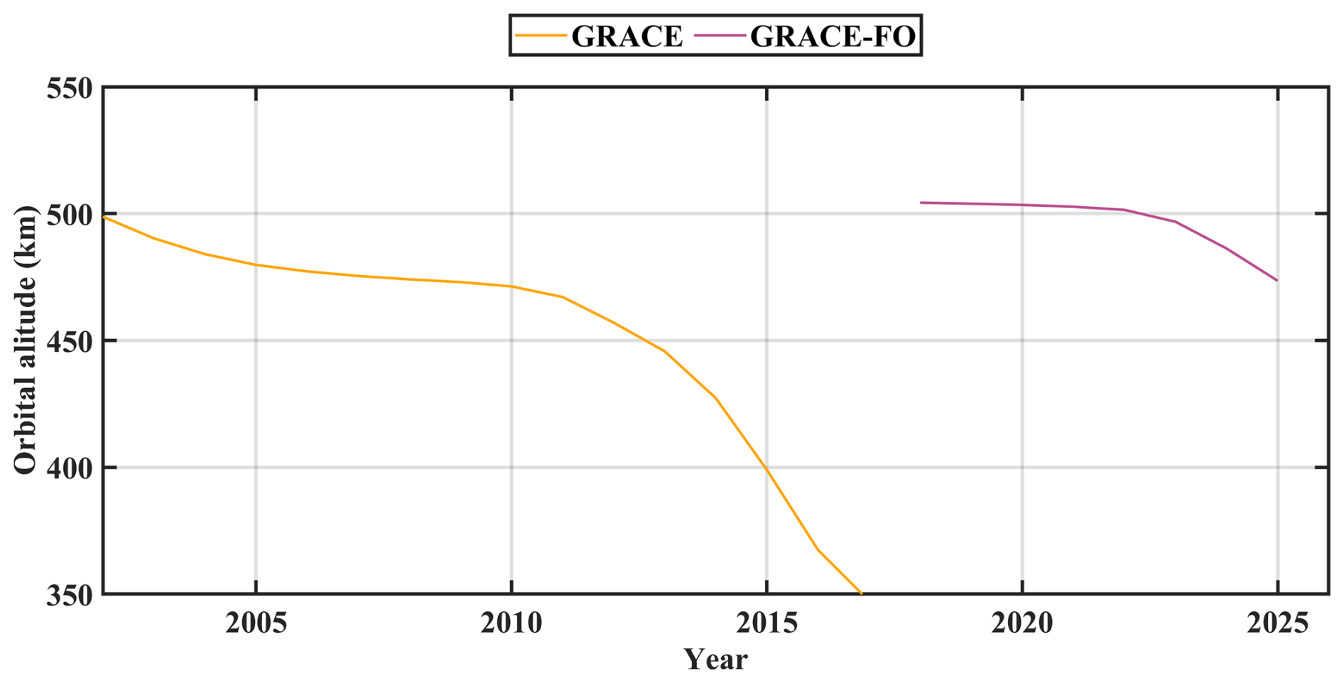
Figure 1 The variation of orbital altitude for satellites during GRACE/GRACE-FO mission operation. Note that the left part of the figure is about GRACE mission which spans from April 2002 to June 2017 while the right part of the figure is about GRACE-FO mission which spans from June 2018 to March 2025.

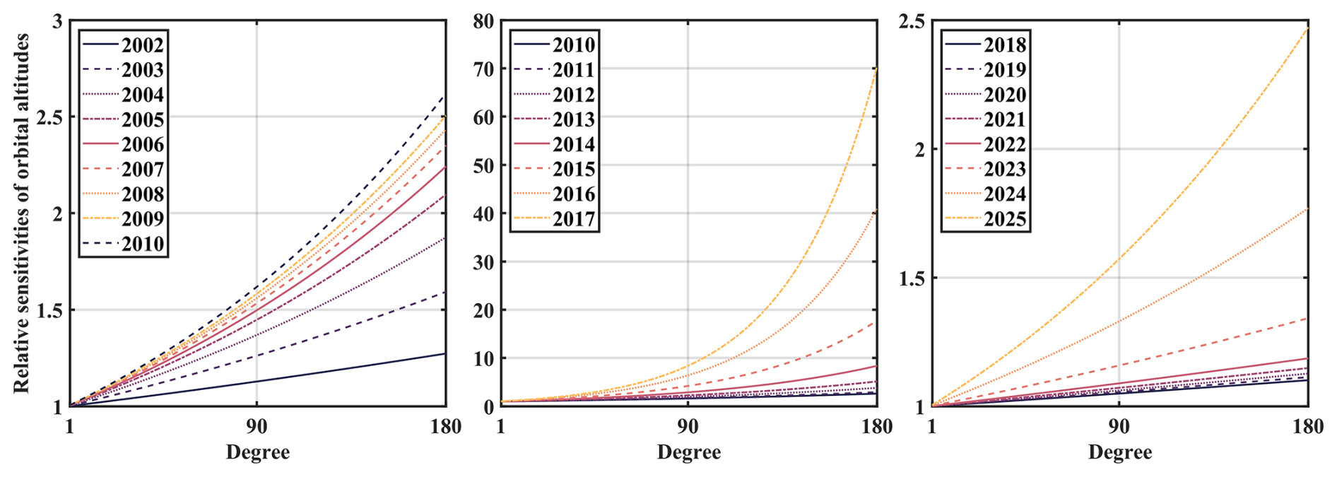
Figure 2 The variation of relative sensitivities of orbital altitudes derived from the GRACE/GRACE-FO precise orbit data GNV1B. Note that the different y axis scale between the left, middle, right figure.

Therefore, the conclusion that GRACE-FO data offer limited additional value is contingent on the processing chain remaining unchanged as shown in Figs. 1 and 2. To address this specific point and move beyond this limitation, we have developed the HUST-Grace2026s solution by introducing several key enhancements to our processing chain, with the objective of improving upon previous models like HUST-Grace2016s.

2.2 Stochastic model and its impact

In the processing of HUST-Grace2026s, we apply a stochastic model based on autocorrelation coefficients from post-fit residuals (i.e. Guo et al., 2018; Chen et al., 2019), rather than relying solely on empirical range-rate parameters. This approach mitigates the 1-CPR effect in KBR1B/LRI1B data. The stochastic model is defined as Eqs. (2)–(4) and the final gravity field solution can be derived from Eq. (5).

$$\begin{array}{}\text{(2)}& {\displaystyle }\mathbf{Q}=\left(\begin{array}{cccc}{\mathit{\rho }}_{\mathrm{0}}& \mathrm{\cdots }& {\mathit{\rho }}_{n-\mathrm{1}}& {\mathit{\rho }}_n\\ \mathrm{⋮}& {\mathit{\rho }}_{\mathrm{0}}& \mathrm{\cdots }& {\mathit{\rho }}_{n-\mathrm{1}}\\ {\mathit{\rho }}_{n-\mathrm{1}}& \mathrm{\cdots }& \mathrm{\ddots }& \mathrm{⋮}\\ {\mathit{\rho }}_n& {\mathit{\rho }}_{n-\mathrm{1}}& \mathrm{\cdots }& {\mathit{\rho }}_{\mathrm{0}}\end{array}\right)\text{(3)}& {\displaystyle }{\mathit{a}}_k={\displaystyle \frac{\mathrm{1}}{N_k}}\sum _i{\mathit{s}}_i{s}_{i+k}(\mathrm{0}\le i\le n)\text{(4)}& {\displaystyle }{\mathit{\rho }}_i={\displaystyle \frac{a_i}{a_{\mathrm{0}}}}(\mathrm{0}\le i\le n)\end{array}$$

where a_k denotes kth auto-covariance vector element, ρ_i denotes the normalized autocorrelation vector element, N_k denotes the pairs of post-fit residual elements used for the auto-covariance elements estimation, and i denotes the lag between different epochs in residual series. It should keep in mind that k must be in the interval (0, n), where n is the total number of residual series.

$$\begin{array}{}\text{(5)}& \mathbf{x}=\left({\mathbf{A}}^T{\mathbf{Q}}^{-\mathrm{1}}\mathbf{A}{)}^{-\mathrm{1}}\right({\mathbf{A}}^T{\mathbf{Q}}^{-\mathrm{1}}\mathbf{l})\end{array}$$

where x denotes the gravity field solution parameter (e.g. $\mathrm{\Delta }{\stackrel{\mathrm{‾}}{C}}_{lm}$ and $\mathrm{\Delta }{\stackrel{\mathrm{‾}}{S}}_{lm}$), A denotes the design matrix, l denotes the residual vector during the gravity field determination.

The primary challenge in implementing a stochastic model for a static gravity field, as opposed to a temporal one, is the dramatically larger parameter space. Solving for a static field to degree/order 180, for example, requires inverting a linear system with 32 757 unknowns. This poses a significant computational challenge, as such an operation would be prohibitively memory-intensive and time-consuming. During the gravity field determination, there are two kinds of data: (1) “observation data” is derived from the satellite instruments onboard; (2) “Stimulation data” is derived from background models. Because of the imperfection of the background models and the instruments onboard, the “observation data” is different from “Stimulation data” leading to residual vector l as shown in Eq. (5). It's should keep in mind that the trend/oscillation parameters will not contribute to the calculation residual vector. During the post-fit residual computation in our manuscript, we determine a temporal gravity field at a degree and order 120, in which we can obtain most temporal gravity signal in the “observation data”. The post-fit residual not only represent the noise of the background models and the instrument observation data, but also represent the accuracy of gravity field. It's reasonable to construct the stochastic model based on the post-fit residual. Moreover, the stochastic model derived from Eq. (2) is designed to whiten the a priori residuals. Unlike the determination of monthly time-variable gravity field models, the static gravity field requires determining the Earth's gravity field variations over a long period of time. It's not feasible to obtain the meaningful postfit residual data during the high-degree static gravity field determination process itself.

In order to resolve the problem of obtaining meaningful postfit residual, we adopt such a strategy as follow:

• (1)

  Determine a time-variable gravity field solution at degree 120, which most of the monthly time-variable signal can be obtained by the gravity field solution.

• (2)

  Computing the monthly postfit residual for the observation data of orbit or range-rate according to the Eq. (7):

  $$\begin{array}{}\text{(6)}& {\mathbf{v}}_j={\mathbf{A}}_j\mathbf{x}-{\mathbf{l}}_j\end{array}$$

  where v_j denotes jth arc corresponding postfit residual, A_j denotes jth arc corresponding design matrix, x denotes monthly gravity field solution parameter, and l_j denotes jth arc corresponding residual vector.

• (3)

  Combining all the monthly postfit residual vector based on different time-scale (monthly, yearly, or the completely solution time):

  $$\begin{array}{}\text{(7)}& \mathbf{S}={\left[\begin{array}{cccccc}{\mathbf{v}}_{\mathrm{1}}& {\mathbf{v}}_{\mathrm{2}}& {\mathbf{v}}_{\mathrm{3}}& \mathrm{\cdots }& {\mathbf{v}}_{n-\mathrm{1}}& {\mathbf{v}}_n\end{array}\right]}^T\end{array}$$
• (4)

  The combined post-fit residuals are used to derive the covariance matrix via Eqs. (2)–(4), as implemented in prior studies (Guo et al., 2018).

To evaluate the model's performance, we conduct a closed-loop numerical experiment using GRACE-FO data from January 2019 to June 2023. This validation approach aligns with standards in gravity field assessment (Kvas et al., 2019). The postfit residual is derived from KBR1B data; LRI1B data is not considered in the experiment. It's noted that the normal equation is constructed once a month, and the static gravity field is obtained only after combining all monthly normal equations. So, we try to combine the postfit residual based on different time scale: (1) Monthly data: Only corresponding monthly postfit residual data is used to construct specific monthly covariance matrix Q, in order words, it means that different month has its own covariance matrix during monthly normal equation construction. (2) Yearly data: All postfit residual data of different month but the same year is used to construct specific yearly covariance matrix Q, in other words, it means that different month but the same year uses the same yearly covariance matrix Q during monthly normal equation determination. (3) All data: All postfit residual data is used to construct a unique covariance matrix Q during monthly normal equation determination.

Figure 3 depicts the covariance matrix and normalized autocorrelation vector elements computed by different length of KBR1B postfit residual derived from monthly temporal gravity field products up to degree 120. For a clear demonstration, the covariance matrix named “Yearly data” (derived from the postfit residual spanning from January 2020 to December 2020), “Monthly data” (derived from June 2020), and “All data” (derived from full-period postfit residual spanning from January 2019 to June 2023). There are two outcomes which can be drawn from Fig. 3:

• (1)

  Suppress the off-diagonal covariance with longer postfit data spans: As the time span which used for computing the postfit residuals' autocorrelation function increases, the off-diagonal elements of the covariance matrix Q gradually approach to zero, and the covariance matrix Q increasingly exhibits a “diagonally dominant” characteristic. This phenomenon also indicates that the correlation of postfit residuals in the current monthly temporal gravity field model solutions arises from unmodeled long-period signals, and this correlation can be mitigated by increasing the length of the postfit residual data.

• (2)

  Distortion of the autocorrelation function at short time scales: Due to the correlation of unmodeled long-period signals, the autocorrelation function time series obtained from monthly-scale postfit residuals show components which are unrelated to integer orbital cycles. A clear example is visible at a lag of 1.5 h, which corresponds to one orbital cycle of GRACE-FO (1-CPR, ∼0.18 mHz). While the autocorrelation functions for the “Yearly data” and “All data” cases show a distinct peak at this orbital period, the function for the “Monthly data” case exhibits successive peaks and troughs. This confirms that the periods of the unmodeled residual signals are not synchronized with the satellite's orbital period.

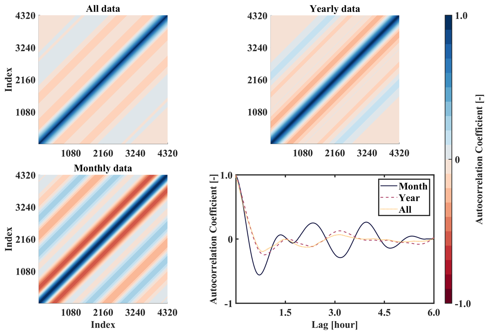
Figure 3 The range-rate covariance matrix and normalized autocorrelation vector element computed by different length of KBR1B postfit residual derived from monthly temporal gravity field determination. The maximum lag of the autocorrelation coefficients series is 6 h, which is consistent with the length of arc during the gravity field determination.

As shown in Fig. 4, the impact of the post-fit residual series length becomes significant beyond degree 40. The differences between the “Yearly” and “Monthly” strategies are most pronounced between degrees 40 and 160. Beyond degree 160, the discrepancy between them diminishes. At degree 180, the geoid height degree differences are 0.19, 0.82, and 0.55 m for the “All”, “Yearly”, and “Monthly” strategies, respectively. The “All” strategy yields a marked reduction in cumulative differences compared to the “Monthly” and “Yearly” strategies, achieving reductions of 66.19 % and 66.67 %, respectively, up to degree 180.

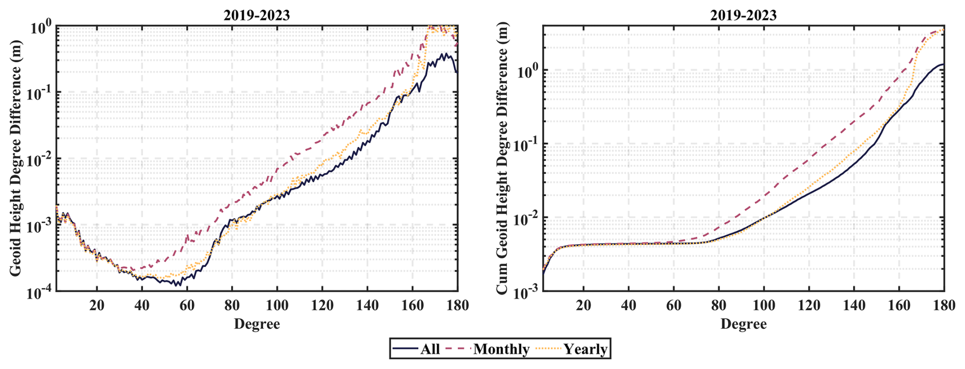
Figure 4 The geoid height difference and cumulative geoid height degree difference between the gravity field model based on different length of postfit residual series and the base model EIGEN-6C4. The postfit residual series is derived from KBR1B data and used to construct covariance matrix at different time scale. The observation data spans from January 2019 to June 2023. Note that the “All” is determined based on a unique covariance matrix, the “Monthly” is determined based on monthly different covariance matrix, the “Yearly” is determined based on yearly different covariance matrix.

2.3 Trend/Oscillation terms estimation and its impact

If we expand the geopotential function at an arbitrary epoch t:

$$\begin{array}{}\text{(8)}& \begin{array}{rl}\mathbf{V}\left(t\right)& ={\mathbf{a}}_{\mathrm{0}}+{\mathbf{a}}_{\mathrm{1}}\cdot (t-t_{\mathrm{0}})+{\mathbf{a}}_{\mathrm{2}}\cos \left({\displaystyle \frac{\mathrm{2}\mathit{\pi }(t-t_{\mathrm{0}})}{T}}\right)\\ & +{\mathbf{a}}_{\mathrm{3}}\sin \left({\displaystyle \frac{\mathrm{2}\mathit{\pi }(t-t_{\mathrm{0}})}{T}}\right)+\mathrm{\cdots }\end{array}\end{array}$$

where V(t) denotes as the geopotential function expanded at epoch t, t₀ denotes as the reference epoch which is always represented by Modified Julian Day (MJD in short), a₀ to a₃ or even more denotes as the estimated parameters. The estimated parameter in this article is a₀ to a₃, which is also represented in terms of normalized spherical harmonic coefficients.

The physical meaning of a₀ is the mean part of the variation of gravity field over a specific time period. However, it's more realistic to take the other parameters (e.g. a₁, a₂ and a₃ according to Eq. 8) into consideration to represent the variation of gravity field during the solution period. Most recent gravity field models published on ICGEM website contain trend/oscillation terms (Ince et al., 2019). As the estimated degree of trend/oscillation terms increase, the heavier computational burden will need to be met. To balance model fidelity and practicality, we implement the estimation strategy based on Kvas et al. (2021), which is widely used during the determination of GOCO series solution (e.g. GOCO06s, Kvas et al., 2021, GOCO2025s, Öhlinger et al., 2025b). Our solution strategies are set as follow: the static coefficients a₀ are solved to degree/order 180, whereas the trend and oscillation coefficients a₁ to a₃ are solved up to degree/order 60. And the reference epoch is set as 2005-06-01 (MJD 53522).

In order to evaluate the performance of the temporal terms (e.g. trend and oscillation parts) during the static gravity field determination, we determine the static gravity field based on GRACE operation period spanning from April 2002 to June 2017 and the geoid difference results with respect to base model EIGEN-6C4 are shown in Fig. 5. The solutions in Fig. 5 – “Static,” “Trend + Static,” and “Nominal” – are generated under three distinct strategies. The “Nominal” solution mitigates the 1-CPR effect solely with empirical range-rate parameters (no combined covariance matrix used in this solution) and no trend/oscillation terms are estimated. In contrast, the “Static” solution uses a combined covariance matrix for 1-CPR mitigation (no empirical range-rate parameters used in this solution) and no trend/oscillation terms are estimated. The “Trend+Static” solution also uses the combined covariance matrix (no empirical range-rate parameters used in this solution) and additionally estimates the complete set of trend/oscillation terms alongside the static field parameters. Significant differences in geoid height degree differences from degrees 2 to 60 are observed between HUST-Grace2016s and the other solutions. This discrepancy stems primarily from their different data spans: HUST-Grace2016s uses data from 2003–2016, while the other strategies use data from 2002–2017. The inclusion/exclusion of data from 2002 and parts of 2017 alters the long-term mean captured by the static solution, leading to variations in the recovered low-degree geopotential coefficients when compared to the base model. The numerical experiments reveal a clear pattern in the cumulative geoid height difference across the strategies. For degrees below 80, all three new processing strategies yield larger cumulative differences than HUST-Grace2016s. Conversely, for degrees above 80, their cumulative differences are consistently smaller. The performance divergence is quantified at degree 160, the cumulative geoid degree difference for “Nominal”, “Static”, “Trend+Static”, and “HUST-Grace2016s” are 7.30, 6.44, 3.81, and 12.60 cm, respectively. Using the “Nominal” strategy as a baseline, the reduction rates of cumulative geoid degree difference for “HUST-Grace2016s”, “Static”, and “Trend+Static” are −72.60 %, +11.78 %, and +47.80 %, respectively. This indicates that applying rate terms reduces cumulative geoid errors by 20.30 % to 51.62 % at degree 180 compared to the nominal strategy.

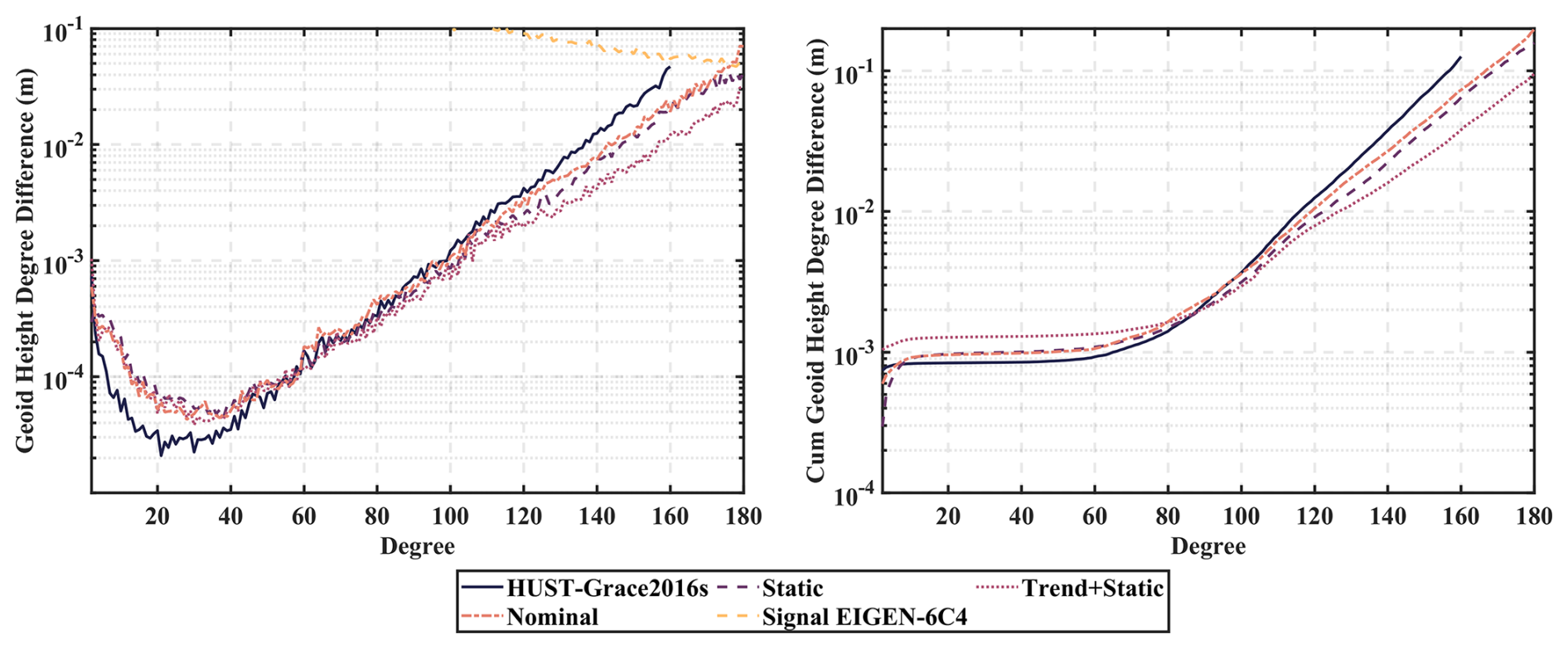
Figure 5 The geoid height difference and its cumulative result derived from different gravity field. All results are derived from GRACE full operation time period spanning from April 2002 to June 2017 except HUST-Grace2016s spanning from January 2003 to August 2016.

The result shown in Fig. 5 also depicts an interesting fact: although the trend/oscillation terms are estimated up to degree/order 60 or the combination of covariance matrix, its contribution starts to be dominant beyond degree 100. This phenomenon may be attributed to high-frequency non-tidal signals, as observed in prior studies (Kvas et al., 2019). Although the error of background models (i.e. AOD1B model or ocean tide model) is remained in the post-fit residual, the covariance matrix is stationary in time domain and can't fully represent the error characteristic of AOD1B or ocean tide model which is more stationary in spatial domain especially. In other words, the contribution of covariance matrix to the gravity field determination is limited (i.e. the difference between “Static” and “Trend+Static” solution in Fig. 5). While the AOD1B product nominally accounts for these signals, residual errors and force model imperfections are not allocated specific parameters for estimation in the pure “Static” processing strategy. Consequently, these unmodeled signals likely persist in the final static solution in the form of aliased frequencies.

To mitigate this issue, four principal approaches are considered according to prior studies:

1. Modelling via trend/oscillation terms: The cumulative effect of the aliased signals can be parameterized using extended rate terms. The advantage of this approach is that the parameter space of the model is intuitive, and the computational code is relatively easy to implement. The disadvantage is that the cumulative effect of frequency-aliasing signals is very complex and requires a large number of parameters to be estimated, which consumes substantial computational resources (Chen et al., 2018).

2. Estimating the daily low-order geopotential: Previous studies have shown that in the AOD1B model, the removed atmospheric and oceanic non-tidal signals mostly follow a 2 or 3 d period, and the daily solutions can significantly reduce the influence of these frequency-aliasing signals (Daras and Pail, 2017). This method addresses the aliasing source directly but depends on external hydrological models as drivers, making its efficacy sensitive to the quality of those input data.

3. Updating the background model: Besides estimating of the daily low-order geopotential coefficients, updating the background model is also an effective approach to reduce the impact of aliasing signal on gravity field determination (i.e. the updating version of AOD1B model, Shihora et al., 2022).

4. Using the model uncertainty estimates: From the view of stochastic model construction, the stochastic model represents the stochastic noise originated from background models and instrument observation data. In other words, the impact of model noise can also be reduced by using the model uncertainty estimation to updating the stochastic model (Kvas et al., 2019; Abrykosov et al., 2023).

3 Result

This paper presents the HUST-Grace2026s static gravity field model, derived from our hybrid processing chain. The solution combines GRACE observations (April 2002–June 2017) with GRACE-FO KBR1B (June 2018–March 2025) and LRI1B (January 2019–June 2023) data. The performance of HUST-Grace2026s is benchmarked against other GRACE-only models through quantitative comparisons involving both gravity field model analysis and external data sources like GNSS-levelling.

3.1 Contribution of GRACE-FO LRI data

3.1.1 Determination based on LRI1B-only

In order to validate the potential of LRI1B data during the static gravity field determination, we perform independent solutions using LRI1B data from four agencies as shown in Table 1. The geoid height differences of the models with respect to base model EIGEN-6C4 are also depicted in Fig. 6. Overall, the geoid height degree difference for solutions determined by different LRI1B datasets are relatively small. The results from AEI, SYSU, and HUST are highly consistent. The JPL result, however, shows slight difference from others between degree 50–70 and degree 100–160. Up to degree 180, the cumulative geoid height difference for AEI, JPL, SYSU, and HUST are 1.17, 1.29, 1.17, and 1.18 m, respectively. Using the JPL result as a reference, the reduction rates of cumulative geoid height difference for the other institutions are 9.3 %, 9.3 %, and 8.5 % (corresponding to AEI, SYSU, and HUST, respectively).

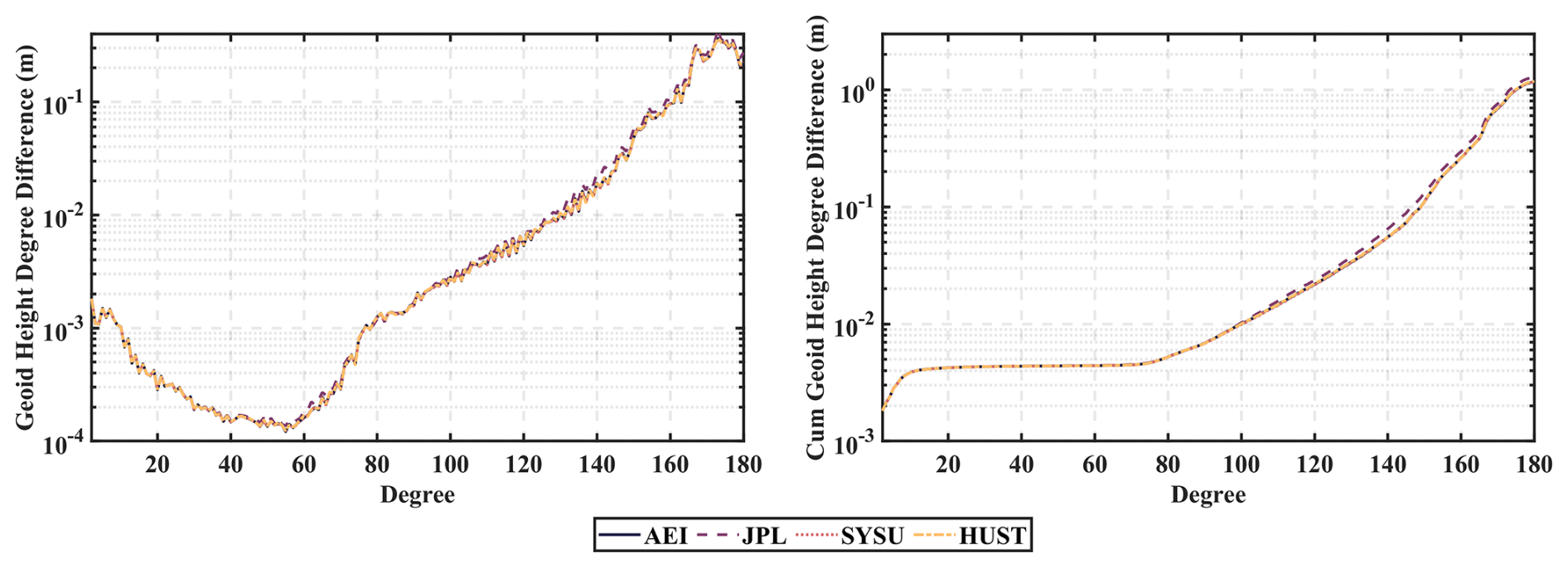
Figure 6 The geoid height difference and its cumulative result derived from static gravity field result with respect to EIGEN-6C4, which is determined based on different agencies' LRI1B data spanning from January 2019 to June 2023. Note that all results in the figure are only determined based on static parameters, and no rate-terms are taken into consideration during the gravity field determination.

Moreover, in order to make a more comprehensive validation for LRI1B-only results, we also calculate the gravity anomaly difference between the LRI1B-only results and EIGEN-6C4 model, as shown in Fig. 7. It is evident that the spatial distribution of gravity anomaly difference for each institution is primarily concentrated within 30° S–30° N. Notably, this pattern is similar to the north-south stripes errors observed in the temporal gravity field models (Chen et al., 2021). The spatial gravity anomaly difference distributions of AEI, SYSU, and HUST are relatively consistent, whereas JPL shows notably larger spatial gravity anomaly difference in regions such as the southern Pacific and southern Atlantic. Following the method mentioned in Chen et al. (2021), we calculate the weighted root mean square (WRMS) of the gravity anomaly differences over the open ocean (defined here as areas more than 300 km from coastlines). The WRMS value of spatial gravity anomaly difference over open ocean for AEI, SYSU, HUST, and JPL are 19.39, 19.57, 19.47, and 21.09 mGal, respectively. Taking JPL's result as a reference, the reduction rates of open ocean spatial gravity anomaly difference for AEI, SYSU, and HUST are 8.06 %, 7.2 %, and 7.6 %, respectively.

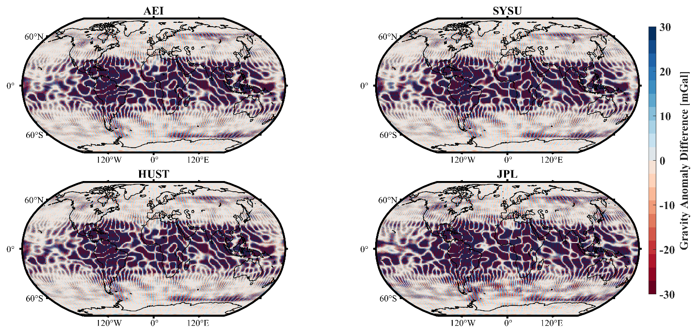
Figure 7 The spatial gravity anomaly difference of static gravity field products, which derived from different agencies' LRI1B data spanning from January 2019 to June 2023, with respect to base model EIGEN-6C4.

3.1.2 Combination with KBR1B data

Building on the validation of LRI1B-only solutions, our primary objective is to determine a global static gravity field model (HUST-Grace2026s) by jointly inverting all available GRACE and GRACE-FO data (KBR1B and LRI1B). A key constraint is that the reference epoch for estimating rate terms (2005-06-01) falls outside the GRACE-FO observation period. To address this and isolate the contribution of LRI1B data, we evaluate its impact under two distinct parameterization strategies: (1) estimating only static parameters, and (2) estimating both static and trend/oscillation parameters. The multi-source data combination is performed using the Variance Component Estimation (VCE) method (Kvas et al., 2021). Although many researchers use the VCE approach to combine the gravity field derived from different observation data source, in our manuscript, the gravity field solution derived from KBR1B or LRI1B has the same error source (i.e. the noise from accelerometer, background models, and so on). In other words, whether the VCE approach is the optimal approach for the combination of gravity field solution from KBR1B and LRI1B still need to be further discussed. Especially, the discussion of optimal approach for combining the solution from KBR1B and LRI1B is out of this manuscript.

The geoid differences relative to EIGEN-6C4 for static solutions under different parameter strategies are shown in Fig. 8 (degree differences) and Fig. 9 (cumulative differences). For static-only estimation (Fig. 8), solutions from different missions vary considerably, a consequence of their disparate data periods. During the GRACE-FO period, solutions agree well up to degree 60. At higher degrees, the KBR-only model is more accurate than the LRI-only model, as the former benefits from a longer time series and higher data redundancy. Merging GRACE and GRACE-FO data yields only a slight improvement in accuracy for degrees 120–140 relative to the GRACE-only solution, with little change or minor degradation at other degrees.

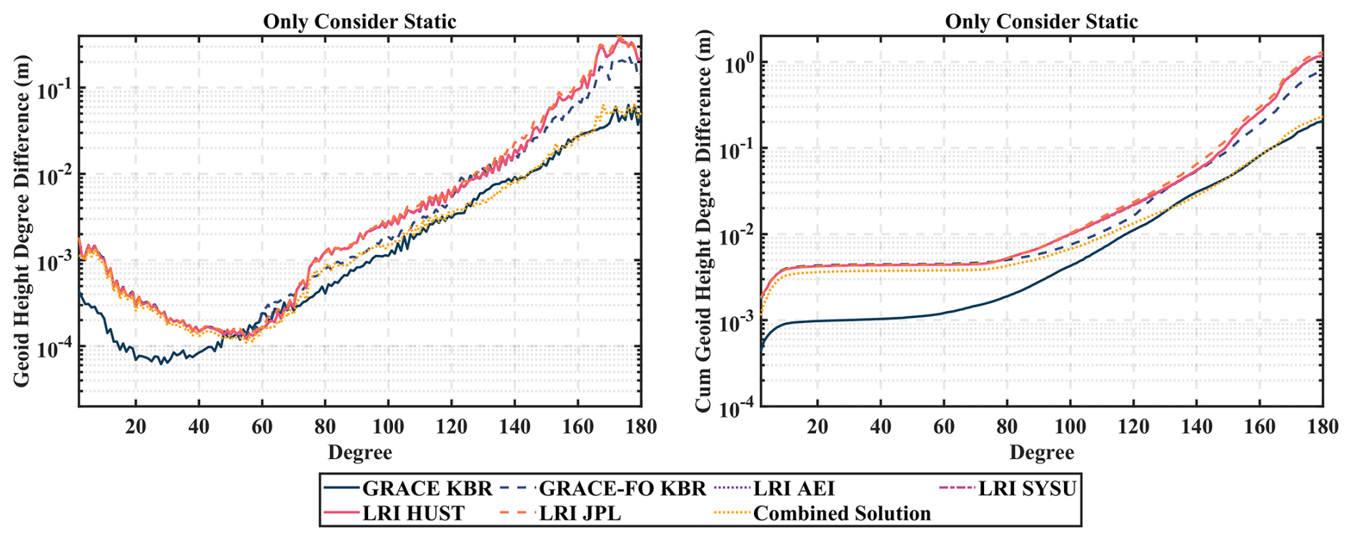
Figure 8 The geoid height difference and cumulative geoid height difference for different static gravity field products with respect to base model EIGEN-6C4. Note that only static part of geopotential coefficients is estimated during the gravity field determination process.

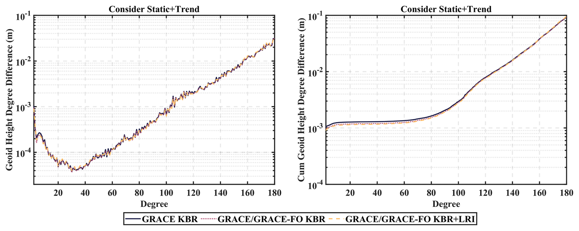
Figure 9 The geoid height difference and cumulative geoid height difference for different static gravity field product with respect to base model EIGEN-6C4. Note that both static part and trend/oscillation terms of geopotential coefficients are estimated during the gravity field determination process. The reference epoch is 2005.06.01.

In contrast to the static-only results (Fig. 8), incorporating trend/oscillation terms alongside static parameters improves the final model accuracy, as previously shown in Fig. 5. However, as shown in Fig. 9, the addition of KBR and LRI observational data from the GRACE-FO satellites does not yield a significant improvement in the precision of the static gravity field models established during the GRACE period. We attribute this to three main factors: (1) Truncation of trend/oscillation terms: In this study, trend/oscillation terms are estimated only up to degree 60. While the LRI data can enhance the accuracy of the Earth's gravity field to degrees much higher than 60 (at least degree 120), extending the trend/oscillation terms estimation to degree 180 would consume substantial computational resources. To balance efficiency and accuracy, we limit the estimation of trend/oscillation terms to degree 60. This truncation may therefore prevent the potential of GRACE-FO LRI data from fully improving the accuracy of static gravity field models under this parameter scheme; (2) Orbital altitude limitation: Unlike the end of the GRACE mission, GRACE-FO satellites currently operate at a higher orbital altitude of about 500 km (as shown in Fig. 1). This reduces its sensitivity to the high-degree geopotential coefficients, making it more challenging to further enhance the accuracy of existing GRACE-based static gravity field without a change in current parameter strategy; (3) Accelerometer data transplantation: In GRACE-FO data processing, accelerometer data from GRACE-C are transplanted to replace the thermally disturbed measurements from GRACE-D. This strategy, while necessary for data continuity, has been shown to degrade the accuracy of temporal gravity field solutions (Behzadpour et al., 2021; Chen et al., 2021), and an analytical framework linking accelerometer noise to errors in geopotential coefficients has been established (Wang et al., 2025). Consequently, the observed limitations in current gravity field accuracy may also be related to this data transplantation approach. However, a focused investigation into its specific implications for static gravity field determination remains outside the scope of this study.

In order to make a further quantitative analysis the result derived from Figs. 8 and 9, we calculate the contribution of data source in the final gravity field determination according to the following equation (Kvas et al., 2021):

$$\begin{array}{}\text{(9)}& {\mathbf{R}}_i={\left(\sum _i{\mathbf{N}}_i\right)}^{-\mathrm{1}}{\mathbf{N}}_i\end{array}$$

where N_i denotes the ith observation data source (GRACE-KBR, GRACE-FO KBR, LRI-JPL, LRI-SYSU, LRI-AEI, LRI-HUST in this article) represented as normal equation, R_i denotes the ith observation data source represented as contribution matrix. Note that all elements in the contribution matrix R ranges from 0 to 1.

To simplify the discussion, the contribution matrices from the four individual LRI products are aggregated into a single “GRACE-FO LRI” dataset. Figure 10, depicting the contribution of each data source to the final VCE-combined model, reveals a complementary weighting pattern: (1) The combination is overwhelmingly weighted towards GRACE KBR and GRACE-FO LRI data. The contribution from GRACE-FO KBR data is marginal, generally between 0.1 and 0.2. (2) GRACE-FO LRI data provides the principal constraint on zonal and near-zonal harmonic coefficients, with contributions of 0.7–0.8 up to about degree 90. GRACE KBR data, while providing a comparable contribution to zonal coefficients, is the dominant source for tesseral and sectorial coefficients at degrees 160 and above. Notably, for certain tesseral coefficients above degree 90, the contribution from GRACE-FO LRI data is substantially higher (∼0.9) than that from GRACE KBR data.

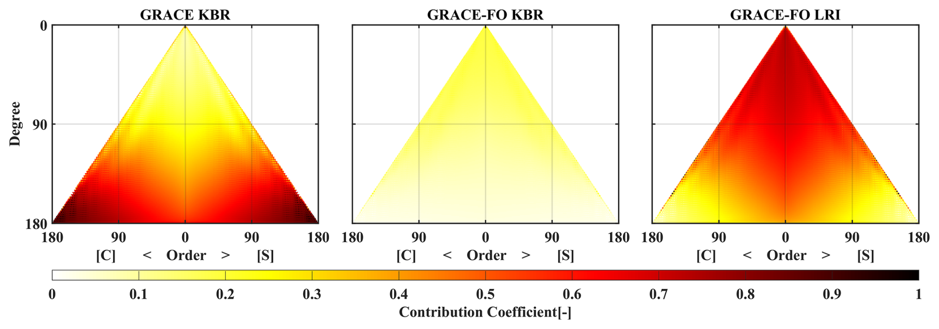
Figure 10 The contribution matrix derived from different normal equations, which are obtained from serval kinds of range-rate data for GRACE and GRACE-FO. Note that all results in this figure are estimated based on static-only parameters estimation strategy during the static gravity field determination.

Figure 11 presents the contribution matrix for the static gravity field model when both static and trend/oscillation terms are estimated. A distinct boundary at degree 60 is evident, resulting from residual correlations between the static and (reduced) trend/oscillation terms that cannot be fully eliminated in the contribution calculation. Compared to the static-only case, the inclusion of trend/oscillation terms lead to a fundamental shift in how the data sources are weighted. This shift is characterized by two main trends: (1) Dominance of GRACE data: GRACE data become the predominant contributor, consistently providing over 60 % of the constraint for most coefficients. This contribution exceeds 0.85 for the geopotential coefficients up to degree 60. Conversely, the contributions from both GRACE-FO KBR and LRI data decline relative to the static-only scenario. (2) Redefined roles at high degrees: The contribution of GRACE-FO KBR data to coefficients beyond degree 90 drops below 0.1. The contribution of GRACE-FO LRI data for degree beyond 60 diminishes gradually from the zonal coefficients outward, falling from a maximum of about 0.4 to about 0.1. This pattern is inversely mirrored by GRACE data, whose contribution increases from about 0.6 near the zonal coefficients to over 0.9 for the surrounding tesseral coefficients. In order to make further research on the change on Figs. 10 and 11, we plot the contribution matrix for the trend parameters as shown in Fig. 12 (the contribution matrix for the oscillation parameters is similar to the trend parameters, but not shown in this manuscript). In this Figure, the contribution of GRACE-FO LRI for trend parameters is slightly higher than that of GRACE-KBR (i.e. 0.5 for GRACE-FO LRI and 0.2 for GRACE KBR). More importantly, the sum of contribution of GRACE KBR for static and trend parameters is near to 1.0. In other words, the contribution for static and trend parameters is not independent but correlated if no regularization information is introduced between static and trend/oscillation parameters during the gravity field determination.

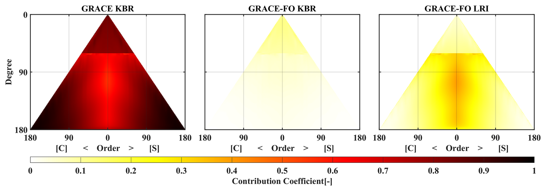
Figure 11 Similar to the Fig. 10, but one should be noted that all results in this figure are estimated based on both static and trend/oscillation terms parameters estimation strategy during the static gravity field determination. Here is the contribution for the static parameters.

Figure 12 Similar to the Fig. 11, here is the contribution for the trend parameters.

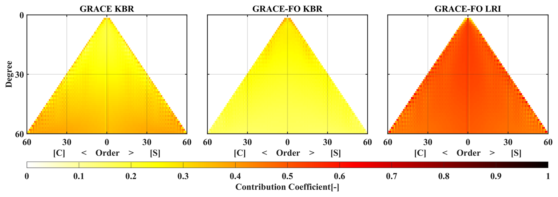
Our findings confirm that adding trend/oscillation terms markedly improve the accuracy of models previously limited to static terms. However, they also reveal two important facts: (1) if the maximum degree for trend/oscillation parameter estimation is set too low, the GRACE-FO LRI data may not confer its maximum possible benefit to the static field determination. (2) The contribution of static parameters has a strong connection with that of trend/oscillation parameters and it should be introduced some prior information to decorrelate them during the static gravity field determination. In other words, it should keep in mind that our result presented in this section is conditional and dependent on the parameter strategies framework.

3.2 HUST-Grace2026s Model validation

3.2.1 Internal validations

To assess the internal accuracy of the combined GRACE/GRACE-FO model HUST-Grace2026s, we compute the differences in its geopotential coefficients relative to the EIGEN-6C4 base model. For further evaluation of internal consistency, we compare it with several established GRACE-only gravity field models: HUST-Grace2016s, ITU-Grace16, Tongji-Grace02s, ITSG-Grace2018s, and GGM05S (Zhou et al., 2017; Akyilmaz et al., 2016; Chen et al., 2018; Kvas et al., 2019; Tapley et al., 2013). Figure 13 presents the corresponding geoid height degree differences and their cumulative sums for all these models (notably, HUST-Grace2026s is the only one incorporating GRACE-FO data).

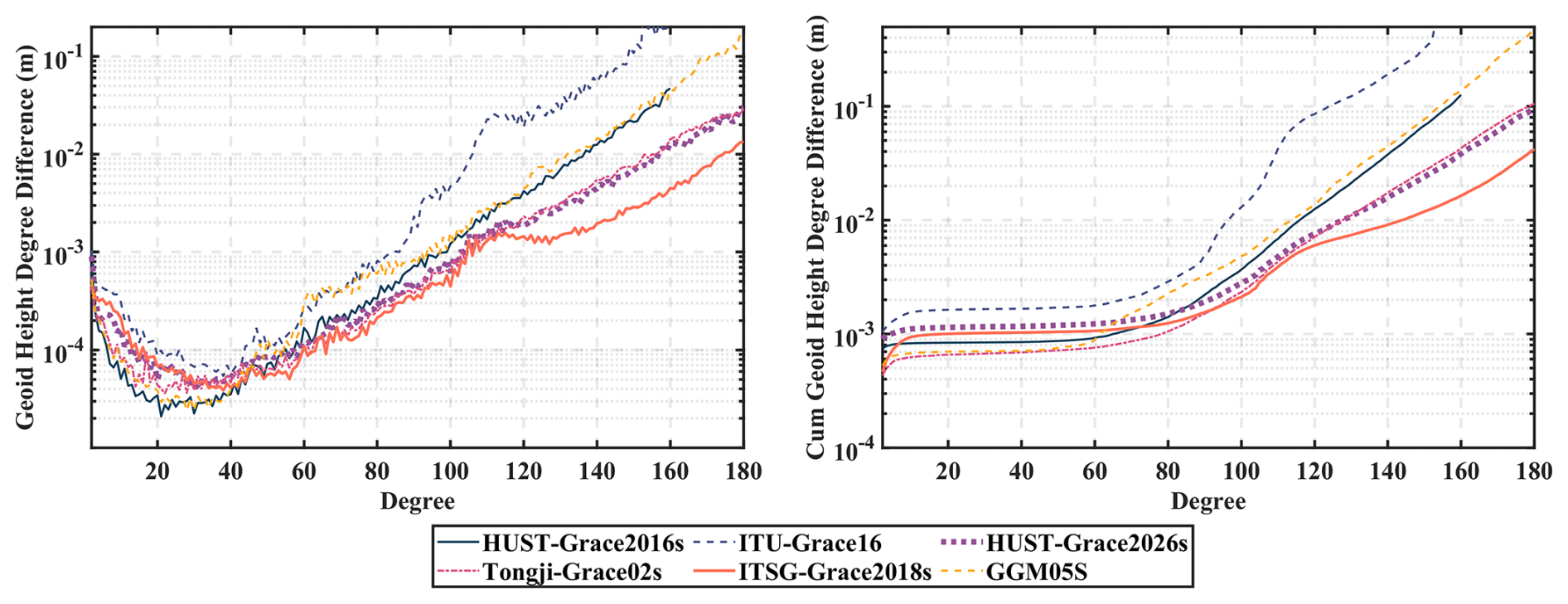
Figure 13 The geoid height degree difference and cumulative geoid height degree difference obtained from different static gravity field products with respect to base model EIGEN-6C4.

The result in Fig. 13 indicates: (1) The significant differences in geoid degree height differences can be observed below degree 40. This primarily stems from their use of observational data spanning different time periods, resulting in inconsistent reference epochs for the static solutions. Consequently, the low-degree discrepancies reflect the variance in the long-wavelength gravity signal captured over each model's unique computation period relative to the fixed reference model. (2) Beyond degree 40, the interplay between the Earth's long-wavelength gravity signal and model noise becomes the dominant factor. As the degree increases, the gravitational signal weakens, allowing model noise and methodological limitations to have a more pronounced effect. This is clearly illustrated by the disparate performance of the different models: The geoid degree differences for ITU-Grace16 increase rapidly with degree, exceeding 0.2 m by degree 160, which can be attributed to limitations inherent in its inversion methodology. The GGM05S spectrum shows a distinct “bump” between degrees 60–80, a potential indicator of over-parameterization during its determination. For other degrees, its accuracy is similar to but slightly lower than HUST-Grace2016s up to degree 160. Tongji-Grace02s, which accounts for perturbing forces, star camera errors, and estimates low-degree rate-terms (up to d/o 50), shows a marked improvement over HUST-Grace2016s from degree 60 onward. HUST-Grace2026s, which incorporates stochastic modelling and rate-terms, achieves overall accuracy comparable to the high-performing Tongji-Grace02s. Tongji-Grace02s's geoid degree difference curve is only marginally higher between degree 120–180.

This last point warrants emphasis: although HUST-Grace2026s incorporates GRACE-FO data in addition to GRACE data, its final accuracy is comparable to the GRACE-only Tongji-Grace02s model. This finding aligns with our earlier analysis concerning the sensitivity of gravity field coefficients to orbital altitude. At the time of this study, GRACE-FO operates at an altitude (∼500 km) comparable to the early phase of the GRACE mission. Consequently, its data exhibit limited sensitivity to the higher-degree coefficients of the Earth's gravity field. Therefore, simply adding GRACE-FO observations under the current orbital configuration does not translate into a significant improvement in the inversion accuracy for these high-degree terms.

A notable feature in Fig. 12 is the superior performance of ITSG-Grace2018s beyond degree 120 compared to both HUST-Grace2026s and Tongji-Grace02s, characterized by a distinct “decline-rise” transition near that degree. This advantage stems from fundamental differences in parameterization and constraint strategies. Unlike the strategies employed in our study and in Tongji-Grace02s, ITSG-Grace2018s adopts a more comprehensive approach: it estimates not only static terms up to degree 200 but also a full suite of trend/oscillation terms to the same maximum degree (Kvas et al., 2019, 2021). More importantly, it applies regularization constraints specifically to the high-degree trend/oscillation terms (beyond degree 120). For the details of the constraints, please refer to Kvas et al. (2021) and Save et al. (2016). This tailored constraint mitigates ill conditioned and enhances the recovery accuracy of high-degree geopotential coefficients. The parameter strategy for HUST-Grace2026s is guided by three principal objectives: to establish a consolidated GRACE-only static field as a baseline, to clearly isolate and evaluate the contribution of GRACE-FO LRI data, and to maintain computational tractability. Therefore, in this solution, the estimation of trend/oscillation terms was truncated at degree 60, and no external prior constraints were applied to decorrelate the static parameters and trend/oscillation parameters. This design choice explains why the coefficient accuracy of HUST-Grace2026s at degree beyond 120 is lower than that of ITSG-Grace2018s, while its overall performance remains comparable to Tongji-Grace02s, which follows a similar estimation strategy.

For a more comprehensive validation, we also calculate the spatial gravity anomaly difference for the GRACE-only static gravity field including HUST-Grace2026s with respect to EIGEN-6C4 as shown in Fig. 14. It should be noted that owing to its maximum truncated degree, the result for HUST-Grace2016s is truncated at degree 160, whereas other models are all evaluated up to degree 180. The result in Fig. 14 indicates serval key points: (1) The global distribution of gravity anomaly differences for ITU-Grace16 or GGM05S is the most pronounced while that of ITSG-Grace2018s is least pronounced, signifying its closest agreement with EIGEN-6C4 and minimal residual noise. (2) The spatial distributions for HUST-Grace2026s and Tongji-Grace02s are relatively similar; however, a notable discrepancy exists near the southwestern Antarctic Ocean, where Tongji-Grace02s shows substantial residuals absent in HUST-Grace2026s, potentially due to their different reference epochs. (3) The weighted root mean square (WRMS) values over the open ocean quantify these differences: HUST-Grace2016s (2.00 mGal), HUST-Grace2026s (1.78 mGal; 0.60 mGal when truncated to d/o 160), GGM05S (8.71 mGal; 2.18 mGal), ITU-Grace16 (26.88 mGal; 11.68 mGal), Tongji-Grace02s (1.85 mGal; 0.67 mGal), and ITSG-Grace2018s (0.72 mGal; 0.25 mGal). These WRMS values (with parenthetical figures representing the consistent d/o 160 truncation for comparative purposes) confirm that HUST-Grace2026s achieves a marked improvement over its predecessor and delivers accuracy comparable to the high-performing Tongji-Grace02s model.

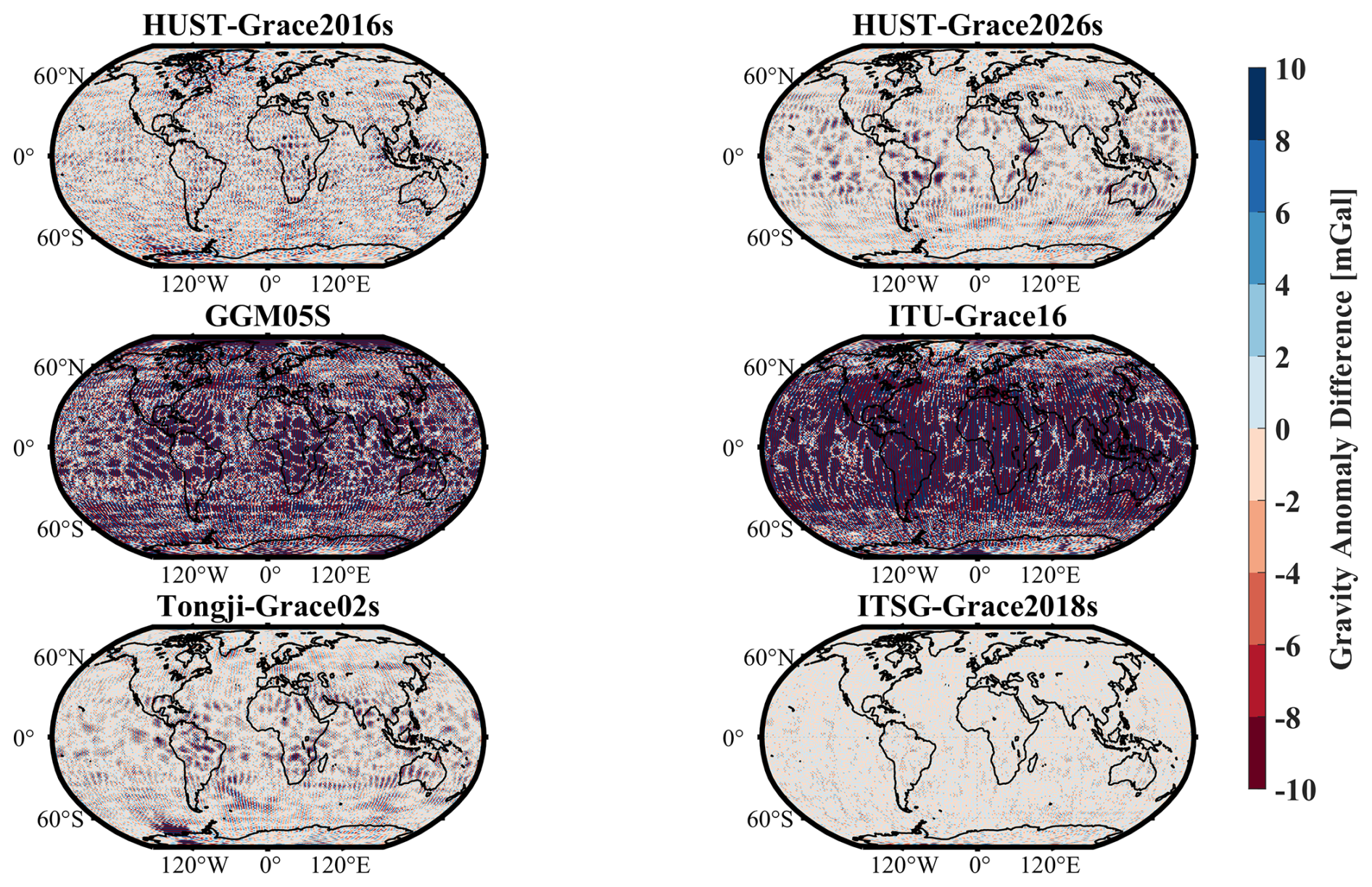
Figure 14 The spatial gravity anomaly difference obtained from different GRACE/GRACE-FO only static gravity field products with respect to EIGEN-6C4. Note that due to the different truncated degree and order of the static gravity field, the spatial gravity anomaly difference of HUST-Grace2016s is calculated up to degree 160, while other models are all calculated up to degree 180.

3.2.2 External validations

The preceding validation assesses model accuracy through direct comparison with a base gravity field model (EIGEN-6C4), an approach hence termed internal validation. For a more robust and independent assessment, an external validation against distinct data sources – such as GNSS-levelling and satellite altimetry-derived marine gravity data – is essential. A critical consideration is that the gravity field models evaluated here are truncated at a relatively low degree (160–180), operating in a different spectral band than these external datasets. To minimize the omission error arising from this truncation, the spherical harmonic coefficients beyond each model's maximum degree are filled using corresponding values from the high-resolution EIGEN-6C4 model, extended to degree 2190.

Figure 15 presents the geoid height differences in North America between the various gravity field models and independent GNSS-levelling data from the National Geodetic Survey (NGS) – a widely adopted benchmark for external validation. The discrepancies arise primarily from differences in the parameterization strategies of each model. Among them, ITU-Grace16 exhibits the poorest agreement, as evidenced by its extensive red difference distribution across the map. The GGM05S model shows a marked improvement over ITU-Grace16. Notably, the spatial difference patterns of ITSG-Grace2018s, HUST-Grace2026s, and Tongji-Grace02s are highly consistent, with ITSG-Grace2018s performing slightly better in the central and northern regions of the United States.

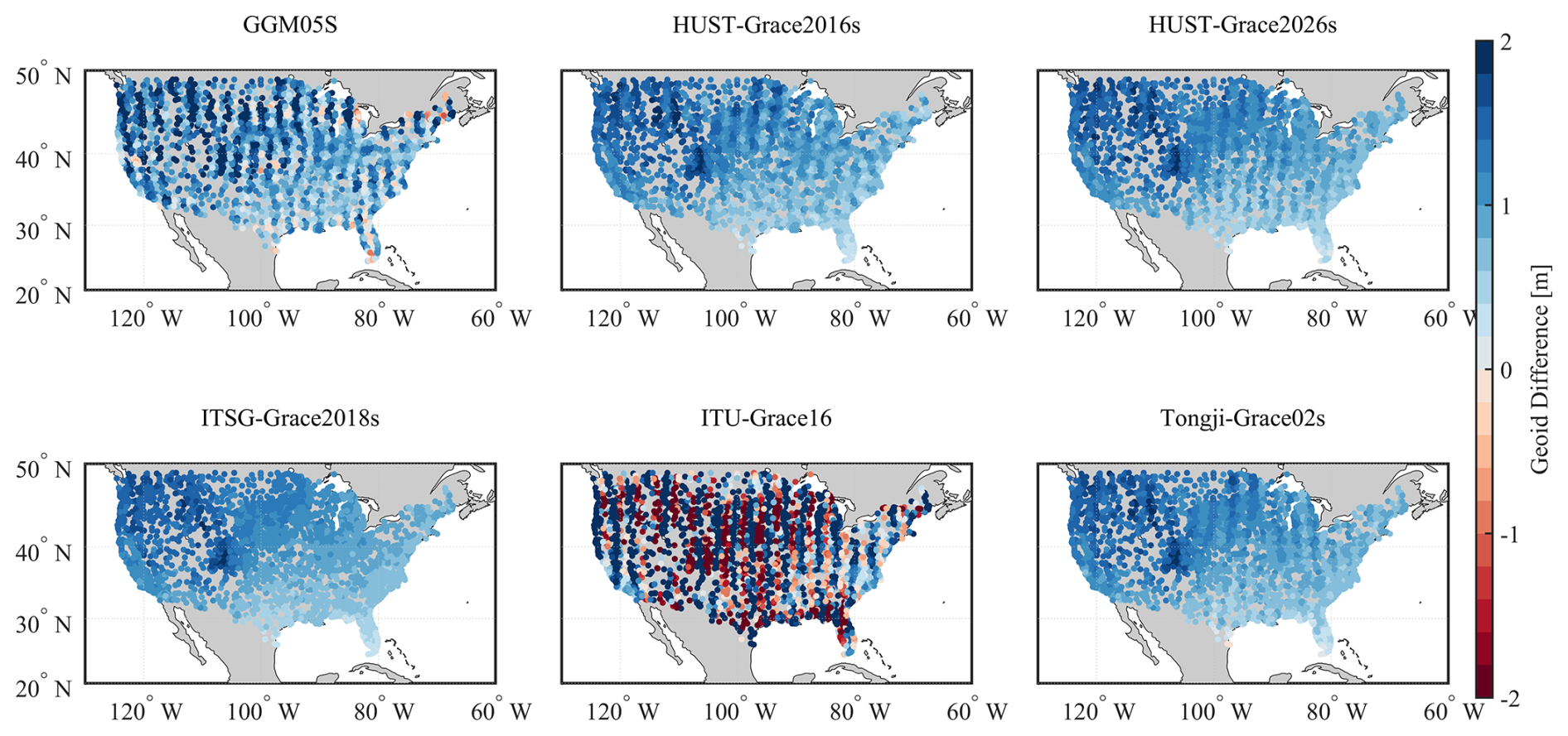
Figure 15 The geoid difference between the result obtained from GNSS Levelling and the result obtained from gravity field models in America.

To quantify the accuracy differences among the models against GNSS-levelling data, we computed the standard deviation of geoid height differences at 20° intervals starting from degree 20, with the results shown in Fig. 16. The statistics reveal two key trends: (1) Below degree 120, the geoid from each gravity field model shows minimal (millimetre-level) deviation from the GNSS-levelling results, indicating that the satellite-derived models cannot resolve the geoid variations captured by the terrestrial data. Beyond degree 120, however, methodological differences and increasing model noise leads to a growing discrepancy. (2) At the maximum degree of 180, ITSG-Grace2018s achieves the smallest standard deviation (0.331 m), while ITU-Grace16 shows the largest (2.644 m). Using ITU-Grace16 as the baseline, the relative reductions in standard deviation for GGM05S, ITSG-Grace2018s, Tongji-Grace02s, and HUST-Grace2026s are 73.7 %, 87.4 %, 86.6 %, and 86.9 %, respectively.

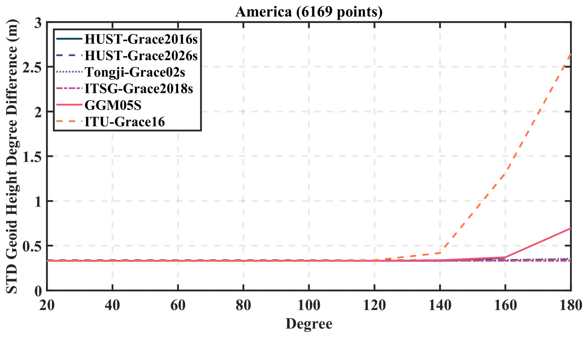
Figure 16 The standard deviation of geoid height degree difference between the results from gravity field models and the results from GNSS Levelling.

In addition to GNSS-levelling, the static gravity field models are further validated against satellite-derived marine gravity data. This study selects the SDUST2022GRA ocean gravity field results as the reference data for external verification (Li et al., 2024). This product encompasses gravity anomaly information for the oceanic regions within 80° S–82° N and 180° W–180° E at an original spatial resolution of ${\mathrm{1}}^{\prime }\times {\mathrm{1}}^{\prime }$. Since the maximum truncation degree of the EIGEN-6C4 gravity field model is 2190-corresponding to an approximate spatial resolution of ${\mathrm{5}}^{\prime }\times {\mathrm{5}}^{\prime }$ – a direct comparison is not feasible. To ensure consistency, the SDUST2022GRA gravity anomaly grid is resampled to a ${\mathrm{5}}^{\prime }\times {\mathrm{5}}^{\prime }$ grid by means of grid averaging firstly. Simultaneously, the geopotential coefficients beyond the maximum degree of each evaluated gravity field model are replaced with the corresponding coefficients from EIGEN-6C4, extended up to degree 2190.

To comprehensively evaluate the accuracy of the gravity anomaly grids derived from the different models, the spherical harmonic expansion of each model is truncated at successive intervals of 20°. Beyond each truncation degree, the coefficients are again filled with those from EIGEN-6C4. The standard deviation of the differences between each resulting grid and the resampled SDUST2022GRA is then calculated, as presented in Fig. 17. Furthermore, three specific oceanic regions are selected for detailed regional comparison: Region 1 in the South Pacific (40–50° S, 130–140° W), Region 2 in the North Atlantic (15–25° N, 40–50° W), and Region 3 in the South Indian Ocean (20–40° S, 70–88° E).

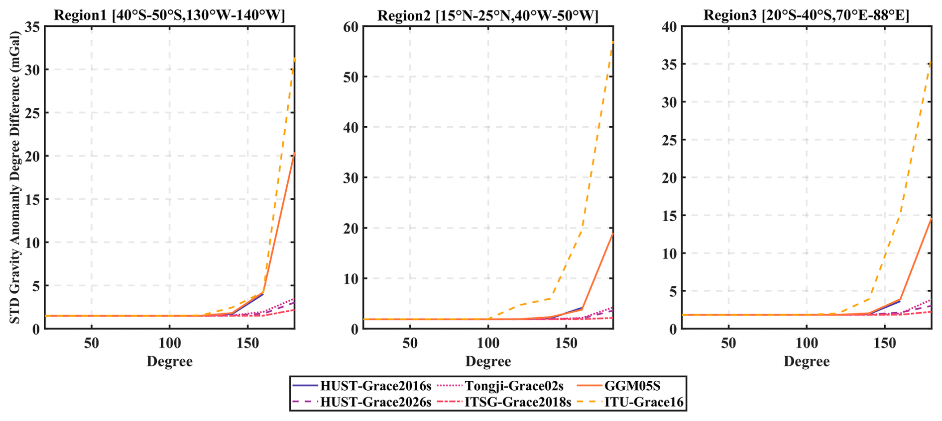
Figure 17 The Standard deviation of gravity anomaly difference between the results derived from gravity field and the results obtained from SDUST2022GRA marine gravity anomaly grids products.

Similar to the GNSS-levelling evaluation, the gravity anomaly grids from all models exhibit minimal divergence from the reference data at low truncation degrees (below degree 100), with the standard deviation of differences remaining stable. A distinct transition occurs beyond degree 140, where discrepancies appear and grow markedly with increasing degree. This rapid increase reflects the growing dominance of residual noise within the models at higher degrees.

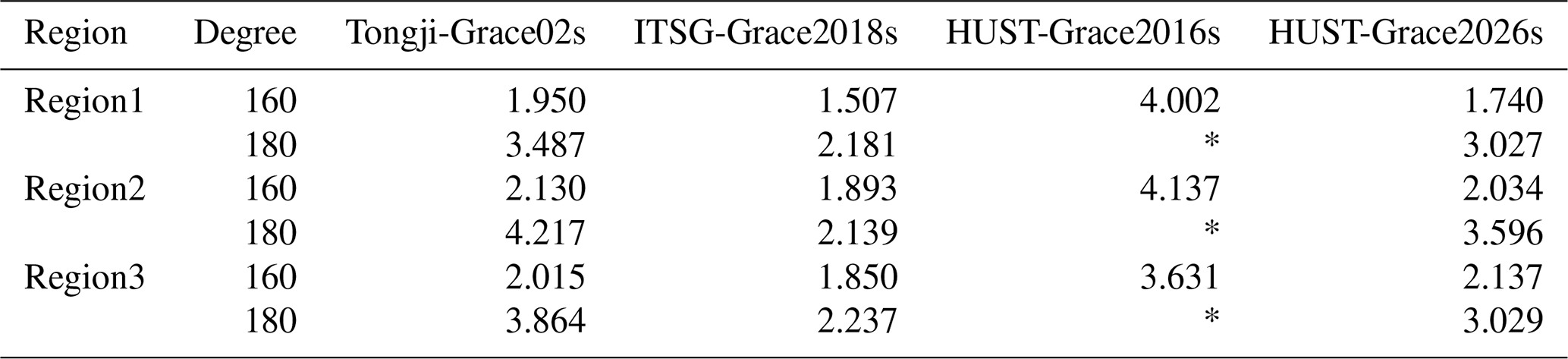
Furthermore, we computed the standard deviation of gravity anomaly differences between the SDUST2022GRA reference and four models – HUST-Grace2016s, Tongji-Grace02s, ITSG-Grace2018s, and HUST-Grace2026s – as summarized in Fig. 17 (Table 2). The analysis reveals two key findings. First, the enhanced processing strategy of HUST-Grace2026s yields substantially higher accuracy than its predecessor, HUST-Grace2016s. When both are truncated at degree 160, the new model reduces the gravity anomaly error by 56.2 %, 52.8 %, and 41.1 % in the three test regions, respectively. Notably, even when extended to degree 180, HUST-Grace2026s still achieves a lower standard deviation than HUST-Grace2016s truncated at degree 160. Second, among the models compared, ITSG-Grace2018s delivers the best agreement with the reference data at degree 180, with standard deviations of 2.181, 2.139, and 2.237 mGal across the three regions. While the corresponding values for HUST-Grace2026s are higher (3.027, 3.596, and 3.029 mGal), it consistently outperforms the similarly formulated Tongji-Grace02s model, achieving accuracy improvements of 13.1 %, 14.7 %, and 21.6 %, respectively.

Table 2 The Standard deviation of gravity anomaly difference between the results obtained from gravity field models for different degree and the results derived from SDUST2022GRA. Note that “*” indicate there is no result provided with the gravity field.

4 Data availability

The GRACE Level 1B data in this study are freely available at https://isdc-data.gfz.de/ (Wen et al., 2019, last access: 27 August 2026), the marine gravity field SDUST2022GRA is available at https://doi.org/10.5194/essd-16-4119-2024 (Li et al., 2024) and the kinematic orbits are provided by ITSG at https://doi.org/10.1016/j.asr.2022.03.014 (Suesser-Rechberger et al., 2022). HUST-Grace2026s model is available at https://doi.org/10.5880/icgem.2026.001 (Zhou et al., 2026b).

5 Conclusion

This study presents HUST-Grace2026s, a new static gravity field model developed using hybrid processing chain that coherently combines observations from the GRACE (April 2002–June 2017) and GRACE-FO (June 2018–March 2025) missions, thereby bridging the gap between these two satellite gravimetry eras and constructing a consistent baseline for long-time mass change variation studies based on satellite gravimetry observation data. The key outcomes of our work are summarized as follows:

1. Impact of GRACE Orbital Altitude: The sensitivity of geopotential coefficients to orbital altitude decay increases with both decreasing altitude and increasing coefficient degree, however, because of the current orbital altitude of GRACE-FO satellite, the contribution of GRACE-FO observation data is still limited for static gravity field determination comparing with that of GRACE. It also confirms the processing chains refinements itself can play a more critical role than the simple addition of current GRACE-FO data.

2. Stochastic Modelling: Employing a long-term residual series for covariance estimation leads to an accuracy improvement exceeding 70 % in most cases compared to the nominal empirical parameter strategy.

3. Contribution of GRACE-FO LRI data: The estimation of trend/oscillation terms up to degree/order 60 primarily enhances the accuracy of coefficients beyond degree 100, yielding up to a 51 % improvement at degree 180. Furthermore, numerical experiments demonstrate that the contribution of LRI data is concentrated in zonal and near-zonal harmonics with full potential realized through adequate parameterization strategies; estimating trend/oscillation terms only to a low degree (e.g., 60) is insufficient to fully exploit the accuracy gains offered by LRI data.

4. Comprehensive Model Validation: Through internal comparisons (against other models) and external validation (using GNSS-levelling and altimetry-derived gravity data), HUST-Grace2026s demonstrates superior performance. It offers a higher spatial resolution (d/o 180) than its predecessor HUST-Grace2016s (d/o 160) and achieves an approximately 50 % noise reduction over oceans. Compared to the current best unregularized solution (Tongji-Grace02s), our model shows an average noise reduction of 10 %–20 %, performing closest to the unregularized static part of the solution ITSG-Grace2018s.