A global base temperature dataset for residential building energy demand modelling

Accurate building energy demand modelling is critical to decarbonizing regional energy systems. The cooling and heating degree-day models are widely used due to their simplicity and low data requirements; however, the lack of accurate base temperature data limits their performance. In particular, the scarcity of high temporal resolution building energy demand data constrains regional-scale base temperature estimation through conventional methods such as the energy signature method and the performance line method. To address this limitation, this study develops a global regional-scale base temperature dataset based on the BiLSTM neural network framework with an attention mechanism. The dataset includes both cooling base temperature (Tcool) and heating base temperature (Theat) for each region, defined at a spatial scale equivalent to a U.S. state or a Chinese province. The BiLSTM framework demonstrates strong performance, with RMSE values of 1.39 °C for training and 1.33 °C for testing, and Pearson correlation coefficients of 0.84 for Tcool and 0.70 for Theat. Predicted results show that global Tcool ranges from 19–25 °C and Theat from 14–18 °C, consistent with physical principles. External validations using 16 independent datasets demonstrate that the predicted base temperatures consistently improve the accuracy of building energy demand modelling, reducing RMSE by approximately 10 % for both cooling and heating, compared to official or empirical base temperatures. This dataset supplements sparse observational base temperature data and enhances the accuracy of building energy demand modelling, contributing to low-carbon energy system planning and broader climate impact assessment. The proposed global Tbase dataset can be acquired from https://doi.org/10.6084/m9.figshare.30646376.v2 (He et al., 2025b).

1 Introduction

Reductions in energy demand and carbon emissions in the building sector play a crucial role in achieving the low-carbon energy system transition and the Paris Agreement climate goals (Camarasa et al., 2022). Buildings accounted for 36 % of global end-use energy and contributed approximately 39 % of energy and process-related CO₂ emissions in 2018, with space heating and cooling representing a major component of total building energy use (UN, 2019). However, building energy demand varies substantially across regions because it is strongly shaped by local climate, ambient temperature, occupant behaviour, and socioeconomic conditions (Deroubaix et al., 2021; Wenz et al., 2017; Staffell et al., 2023). An increase in ambient temperature will reduce heating demand but increase cooling demand across different regions (Abajian et al., 2025; Wang et al., 2023; Filahi et al., 2025; Clarke et al., 2018; Zhou et al., 2013), and identical building configurations exhibit distinct energy demand patterns across different climate zones (Mahdavinejad et al., 2024; Yu et al., 2014). Beyond climate zones, terrain and topography further modulate local microclimate, ventilation, and solar exposure, thereby shaping heating and cooling energy demand and occupant responses (Papada and Kaliampakos, 2016; Zhang et al., 2024a). Occupant responses to temperature changes, such as adjusting clothing, using air-conditioning, or changing activity patterns, further contribute to this spatial heterogeneity (Bae et al., 2025; Gupta et al., 2024; IEA, 2024). Accurate characterization of building energy demand therefore requires approaches that account for regional differences rather than assuming uniform responses across locations.

The degree-day method is one of the most commonly used approaches for modelling heating and cooling energy demand in buildings. Degree-day models exhibit substantial advantages in terms of data availability and geographic generalization when compared to physical and statistical models (Prataviera et al., 2021; Ahmad et al., 2018). The base temperatures define thresholds for heating (below the heating base temperature) or cooling (above the cooling base temperature) in buildings (De Rosa et al., 2015; Martinopoulos et al., 2019). Degree days are calculated as the difference between the average daily temperature and this base temperature, with values below the threshold being the heating degree day (HDD) and those above the threshold being the cooling degree day (CDD). Base temperature values are influenced by local climatic conditions, occupant behaviour, building types, and thermal properties (Ramon et al., 2020; Hao et al., 2022), which suggests significant spatial heterogeneity in base temperature selection. Moreover, base temperature has been linked to indoor thermal comfort, which differs across populations, so the temperature thresholds for initiating heating or cooling vary between regions (Staffell et al., 2023). In the United States, 18.3 °C is the most common base temperature, above which cooling demand is considered to increase and below which heating demand increases (Petri and Caldeira, 2015). In the UK, the HDD and CDD are calculated using 15.5 and 22 °C as the base temperatures, respectively (UK Climate Projections, 2014). In China, 18 and 24 °C are widely used as the base temperatures for the degree-day model (Yang et al., 2024; Li et al., 2018). Conventionally, recommended base temperatures have served as key parameters in modelling heating and cooling energy demand across buildings, regions, and countries (Camarasa et al., 2022; Deroubaix et al., 2021). However, the application of uniform base temperatures across broad geographical areas inadequately represents the sensitivity of building energy demand to local climatic variations, raising concerns about the accuracy and uncertainty of degree-day modelling. To illustrate, a 1 °C change in the base temperature can result in approximately 20 additional or fewer CDDs per month in San Luis Obispo (Woods and Fuller, 2014). Inaccurate base temperatures also trigger a nonlinear relationship between building energy demand and degree days (Day et al., 2004).

Accurate base temperature selection is essential for reliable degree-day modelling. The energy signature approach and performance line analysis are commonly used to determine optimal base temperatures at regional scales by integrating building energy consumption data and local meteorological data (Bhatnagar et al., 2018; Staffell et al., 2023; Anjomshoaa and Salmanzadeh, 2017; Woods and Fuller, 2014). In the energy signature method, energy consumption is correlated with outdoor temperature to identify a non-linear relationship, and the inflection point of the resulting curve is taken as the base temperature (Anjomshoaa and Salmanzadeh, 2017; Meng et al., 2018). The performance line method estimates the base temperature by plotting the best-fit straight line of energy consumption relative to the HDD or CDD (Bhatnagar et al., 2018). A major strength of both approaches is that they use observed energy use that integrates local weather conditions and occupancy behaviour, providing empirically grounded base temperatures for specific regions. For example, Bhatnagar et al. (2018) applied both the energy signature method and the performance line method to determine base temperatures across 60 Indian cities, reporting median base temperatures of 18.3 °C for cooling and 17.4 °C for heating. In Kerman, Iran, the L-curve relationship between average daily temperature and natural gas consumption is derived using the energy signature method, revealing base temperatures of 15.42 and 21.18 °C for the region (Anjomshoaa and Salmanzadeh, 2017). Furthermore, Staffell et al. (2023) evaluated indoor temperature thresholds for heating and cooling across several countries and regions based on the energy signature method. However, these benchmark methods also have important limitations. They typically require building energy consumption data at high temporal resolution together with matched meteorological records, which restricts their application to data-rich regions and makes large scale or global benchmarking costly and impractical. Consequently, although these methods are valuable for local and regional calibration, they cannot be readily extended to produce consistent base temperature estimates across data scarce regions worldwide.

When empirical base temperature calibration is unavailable, regional and global assessments of temperature-dependent building energy demand often rely on harmonized base temperatures rather than locally derived values (e.g., Deroubaix et al., 2021; Scoccimarro et al., 2023; Falchetta et al., 2024). This reliance may obscure spatial heterogeneity in building climate responses and reduce the reliability of degree-day-based energy modelling at broader scales. These challenges highlight the critical need for a practical methodology that can predict base temperatures at a global scale using limited data – a prerequisite for accurate global energy demand modelling. To address this gap, this research develops a global regional-scale base temperature dataset by combining energy demand derived labels from segmented linear regression with a BiLSTM framework incorporating an attention mechanism. Using limited building energy observations together with regional weather and socioeconomic data, cooling base temperature (Tcool) and heating base temperature (Theat) are mapped at provincial resolution and upscaled to continuous global maps. An integrated validation framework is further established to assess the reliability of the predicted base temperatures for building energy demand modelling. The resulting dataset provides spatially explicit base temperature information to support regional energy demand modelling and low-carbon energy system planning.

2 Data and methods

2.1 Data

2.1.1 Energy demand data

The energy demand data encompasses multi-timescale time series electricity or natural gas demand data from 172 regions worldwide (see Table A1). These data are utilized to estimate region-specific base temperatures (Tbase), which serve as critical input data for subsequent analyses. Two types of energy demand are considered: building-level and region-level. Building-level energy demand data predominantly consists of residential demand across various temporal resolutions (second, minute, and hourly intervals), which are aggregated to a daily scale (kWh d⁻¹) to better reflect seasonal patterns linked to local temperatures and weather conditions. Due to the scarcity of available residential data, a small number of public building energy demand datasets are also included to expand coverage. Region-level energy demand data, available at daily and monthly temporal scales (kWh d⁻¹ or MWh per month), can also capture seasonal variations when the time series is sufficiently long, as demonstrated by Wenz et al. (2017), Huang and Gurney (2016), and Staffell et al. (2023). All energy demand datasets are spatially matched to the finest available administrative boundaries using location metadata, thereby enabling integrated analysis with local climatic conditions.

2.1.2 Meteorological variables

Meteorological data are primary drivers of temporal variations in building energy demand. This study utilizes five key variables from the ERA5-Land Reanalysis data (daily or monthly averages from 1950 to present): 2 m air temperature (T2m, K), dew point temperature (Td, K), 10 m u- and v-components of wind (u, v, m s⁻¹), and surface downward solar radiation (SSRD, J m⁻²). The u- and v-components are combined into 10 m wind speed (WS) for analysis. The 2 m air temperature reflects diurnal variations and seasonal trends across a wide range of environments and is strongly correlated with building energy demand (Li et al., 2018; Mishra et al., 2024). Dew point temperature, in relation to air temperature, captures atmospheric humidity variations. In winter, higher humidity enhances thermal comfort at lower temperatures, while in summer, it intensifies perceived heat stress and elevates cooling energy requirements, as occupants tend to set lower setpoint temperatures to achieve comfort (Pawlak et al., 2021; Choi et al., 2017; Mansouri et al., 2023). Wind speed affects the heat transfer process through the building envelope (Cholewa et al., 2021). Higher wind speeds typically increase heating energy demand during winter through enhanced heat losses and may reduce cooling loads in summer due to improved natural ventilation (Hirth et al., 2024). However, the impact of wind speed varies by region, with some areas showing little sensitivity (e.g., Chambers and Oreszczyn, 2019). Solar radiation provides beneficial passive heat gains during winter, thereby reducing building heating needs, but can exacerbate overheating in summer, increasing cooling demand (Huang and Kang, 2021; Zhao et al., 2024).

The spatiotemporal heterogeneity of meteorological variables, combined with the varying sensitivity of building energy demand to different meteorological conditions, adds complexity to the accurate estimation of Tbase. Among these variables, air temperature is the most dominant factor affecting building energy demand, while humidity, wind speed, and solar radiation function as correction terms that modify temperature effects. Their physical interdependence with temperature amplifies the nonlinear dynamics of building energy demand and contributes to the uncertainty in determining Tbase.

Table 1 Description of meteorological variables and static features.

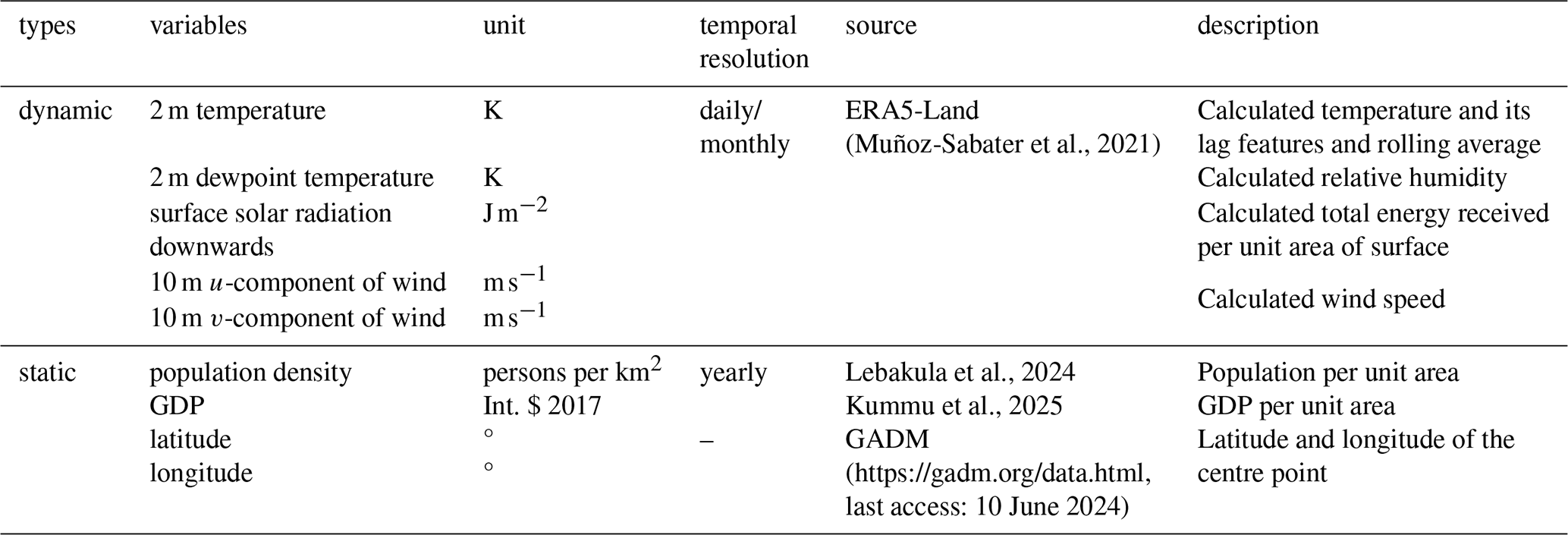
Note: Int. $ 2017: 2017 international dollars (purchasing power parity).

2.1.3 Static features

Static features include socioeconomic variables, along with the geographic coordinates (longitude and latitude) of each region, as shown in Table 1. Population density (persons km⁻²) is critical in shaping regional microclimate through urban densification, which in turn affects thermal comfort. In densely built urban environments, reduced wind speeds in narrow canyons limit heat circulation and removal, thereby worsening thermal conditions (Perera et al., 2023). This degraded thermal environment forces residents to rely more on mechanical cooling during the summer months. In addition, per capita heating energy demand varies substantially across population density ranges (Zarco-Periñán et al., 2021), which reflects the heterogeneous impact of population density on energy demand. Regional affluence, characterized by economic density (GDP per unit area, 2017 int. $ km⁻²), also strongly influences residential energy access and consumption patterns (Rode et al., 2021; Abajian et al., 2025; van Ruijven et al., 2019). Typically, in low-income areas, the adoption of air conditioning is often delayed due to financial constraints (Duan et al., 2023), resulting in higher summer base temperatures. Conversely, in high-income areas, cooling systems are typically activated at lower ambient temperatures. This disparity is particularly pronounced in rural-urban comparisons, where urban populations tend to exhibit lower temperature thresholds for initiating electricity demand (Shi et al., 2025).

Geographic coordinates (longitude and latitude) serve as fundamental determinants of regional climate variability and influence local populations' adaptive behavioural responses to thermal conditions. For instance, residents in high-latitude regions tend to be more acclimated to cold climates and typically initiate heating systems at lower temperatures than those in lower-latitude counterparts (Yilmaz and Canan, 2025).

2.2 Model development

This study developed a novel framework to spatially generate an accurate dataset of base temperatures at the regional scale by integrating a statistical model and a Bidirectional Long Short-Term Memory (BiLSTM)-based neural network framework (Fig. 1a). First, the target data for the training set is prepared by a statistical model. The BiLSTM model is then trained to obtain optimal parameters, incorporating both stratified sampling and an attention mechanism. Stratified sampling ensures a more representative division of the dataset into training and test sets, while the attention mechanism enhances prediction accuracy by automatically focusing on the most relevant time steps for Tbase estimation. The final step is the generation and assessment of Tbase values at the regional scale.

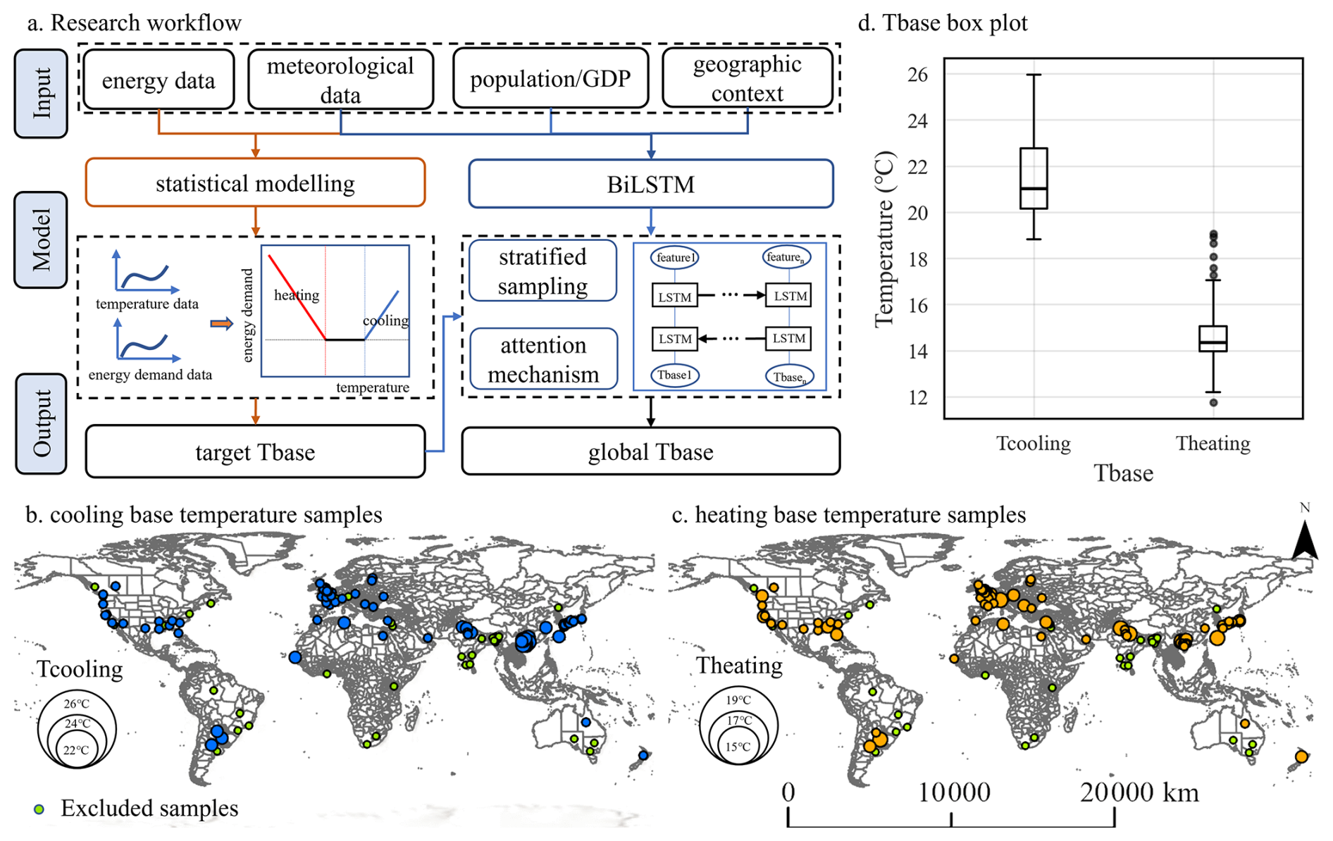
Figure 1 Workflow and Data Preparation. (a) Research workflow based on a segmented linear regression model and BiLSTM; (b) cooling base temperature samples; (c) heating base temperature samples; (d) Box plot of base temperature samples.

2.2.1 Target base temperature data preparation

Two types of base temperature, the cooling base temperature (Tcool) and the heating base temperature (Theat), are used as training targets. These targets are derived from the nonlinear relationship between actual energy demand and outdoor temperature across different regions. To adequately capture seasonal changes in energy use, the time series of daily energy demand should be at least one year long, while monthly energy demand data should be at least five years long. Furthermore, location metadata is essential for each energy demand dataset, as regional climate-energy relationships are critical for accurately estimating spatial variations in Tbase. Detailed information on the datasets used in this research is provided in Table A1.

Regression approaches are used to estimate Tbase values by modelling the relationship between energy demand and outdoor temperature. This relationship can be represented using a variety of specifications, including linear, polynomial, and exponential models (Fung et al., 2006; Ihara et al., 2008; Li, 2018). Although complex nonlinear models can provide precise model fits, they often pose challenges such as overfitting and limited interpretability of parameters, which limits their applicability across diverse regions (Staffell et al., 2023). To address these limitations, this study adopts a segmented linear regression model, grounded in the energy signature method (Bhatnagar et al., 2018), to identify the critical turning points in the energy demand-temperature relationship, namely the cooling and heating base temperatures (Tcool and Theat). The segmented linear regression model is expressed as follows:

$$\begin{array}{}\text{(1)}& E_{ti}=\left\{\begin{array}{ll}a+b_{\mathrm{1}}(\text{Theat}-T_{ti}),& T_{ti}<\text{Theat}\\ a,& \text{Theat}\le T_{ti}\le \text{Tcool}\\ a+b_{\mathrm{2}}(T_{ti}-\text{Tcool}),& T_{ti}>\text{Tcool}\end{array}\right.\end{array}$$

where E_ti represents energy demand at location i on day (or month) t. For daily datasets, E_ti is expressed in kWh d⁻¹; for monthly regional datasets, it is expressed in MWh per month. T_ti denotes the corresponding average outdoor temperature (°C). Theat and Tcool represent the heating and cooling base temperatures at location i (°C), respectively. Coefficients b₁ and b₂ denote the slopes of heating and cooling segments in the energy-temperature relationship. Specifically, b₁ indicates that heating demand decreases as outdoor temperature increases, while b₂ indicates that cooling demand increases with rising temperature. When outdoor temperature T_ti falls between Theat and Tcool, the building does not require active neither heating nor cooling, and the energy demand reflects the baseline load independent of temperature variations. When T_ti<Theat, heating is required to maintain indoor thermal comfort, and when T_ti>Tcool, cooling is necessary.

The segmented linear regression model identifies Tbase values through a three-step process. (1) Determining the number of base temperatures: for each energy-temperature dataset, both two-segment linear regression and quadratic regression are performed. The number of Tbase values is determined by comparing their R² values. When the quadratic regression yields a higher R², the energy-temperature relationship is likely U- or V-shaped, indicating the presence of both heating and cooling base temperatures. Otherwise, only a single Tbase is identified: a positive slope in the non-horizontal segment corresponds to Tcool, while a negative slope indicates Theat. (2) Calculating base temperatures: for datasets with a single base temperature, Tbase corresponds to the breakpoint of the fitted line. For datasets with two base temperatures, the minimum temperature point (Tmin) from quadratic regression is used as a reference. Intervals of (Tmin − 6 °C, Tmin) and (Tmin, Tmin + 8 °C) are examined at 0.05 °C increments to search for two breakpoints maximizing the R² of a three-segment linear regression, and the resulting breakpoints are identified as Theat and Tcool, respectively. The search intervals were set empirically, with a wider margin on the cooling side to accommodate more diverse active cooling responses. All detected Theat and Tcool values fell within these intervals rather than at their boundaries, indicating that the chosen range is sufficiently wide to capture the true breakpoints without truncation. (3) Producing the target dataset: detected Tbase values are retained only if the segmented regression achieves an R² above 0.5, ensuring an adequate model fit, and if the resulting Theat and Tcool values are physically plausible (i.e., Theat<Tcool, and both values fall within typical comfort temperature ranges of 10–30 °C). Ultimately, base temperature values from 131 out of 172 geographical units are included in the final labeled dataset, as shown in Fig. 1b–d and Table A2.

Building-level energy demand datasets require careful pre-processing prior to segmented linear regression to ensure reliable analysis. For each dataset, three pre-processing steps are performed: (1) The energy demand time series for each building is visualized to exclude those without cyclical variation patterns, as such buildings typically exhibit temperature-independent demand (e.g., warehouses) (Staffell et al., 2023); (2) Daily energy demand of all buildings within each geographical unit are aggregated and averaged to represent regional building energy demand; (3) Using two-dimensional energy-temperature data, a density-based clustering method is used to eliminate abnormal daily records, which are often the results of data errors or abnormal demand patterns due to holidays. For region-level datasets, only outlier detection is performed, as their monthly temporal resolution naturally smooths out short-term fluctuations such as holiday effects.

2.2.2 Model training

The model has been trained using Tbase values and corresponding feature data from 131 geographic units. Monthly-scale meteorological data are chosen as dynamic features because their temporal smoothing effectively filters out high-frequency noise while retaining medium- and long-term trends. These retained signals are more strongly correlated with energy demand and Tbase, enabling the model to capture more stable physical relationships and enhance spatial generalization.

Weather data exhibit complex time-series characteristics, including cyclical patterns, seasonal variations, and long-term trends, which are closely linked to variations in occupant energy demand for cooling and heating across different regions. To address the temporal complexity of meteorological data and their nonlinear relationships with energy demand, this study constructs a neural network framework based on a Bidirectional Long Short-Term Memory (BiLSTM) architecture to model the relationship between time-series weather data and Tbase (Fig. 1a).

LSTM networks represent an advancement over traditional recurrent neural networks (RNNs), effectively addressing the fundamental challenge of preserving information across extended sequences – also known as long-term memory capacity, which makes them particularly well suited for processing time-series data (Hochreiter and Schmidhuber, 1997). Each LSTM cell integrates three gates (input, forget, and output) and a storage unit (Zhang et al., 2024b). The input gate regulates how much new information is added to the memory. The storage unit preserves historical information across time steps, enabling the network to maintain long-term dependencies. The forget gate determines which information is discarded, while the output gate determines which information is passed on to the next hidden state (Kim et al., 2024b; Chen et al., 2023). By controlling whether to retain or discard information, LSTM networks mitigate the vanishing and exploding gradient problems that commonly affect traditional RNNs during training.

The BiLSTM model extends the standard LSTM by processing input sequences in both forward and backward directions (Schuster and Paliwal, 1997; Palazzoli et al., 2025). This bidirectional architecture captures temporal dependencies more comprehensively, enabling the model to learn complex patterns from both past and future contexts in historical weather data. The forward processing captures the temporal evolution of weather patterns, while the reverse processing identifies important contextual relationships that may be missed in a unidirectional processing. By leveraging this full temporal context, the BiLSTM model yields more accurate estimates of Tbase values.

In the BiLSTM framework, monthly meteorological data at the regional level and annual socioeconomic data by region from 2000 to 2020, as well as latitude and longitude, are used for model training. For dynamic features, sequence normalization is applied within each geographic unit to preserve the periodicity and seasonality inherent in meteorological variables. For static features, global standardization across all units is performed to highlight absolute differences between geographic units. Furthermore, latitude and longitude are encoded to capture rich location information. A sequence length of 24 months is chosen, which provides a balance between capturing patterns of climate variability and maintaining a sufficient number of training samples. An attention mechanism is applied to the BiLSTM outputs, assigning learnable weights across time steps so that months more relevant to the base temperature contribute more to the aggregated temporal representation; a residual connection is added to stabilize training. To address the issue of sparse and unevenly distributed samples, K-means clustering is applied using geographic coordinates (latitude and longitude) to classify the 131 geographic units into three clusters. Training and test sets are then constructed proportionally within each cluster, ensuring stratified sampling and preserving the geographical representativeness of the training set – thus enhancing the model's capacity for spatial generalization. The final train-test split follows an 8:2 ratio. To prevent data leakage, all sequences from each geographic unit are assigned exclusively to either the training or test set. Model training adopts an early stopping strategy, halting if no improvement is observed over 20 consecutive epochs, with a maximum of 50 epochs.

The mean squared error (MSE) is used as the loss function, which is particularly sensitive to large errors and thus encourages the model to minimize substantial prediction biases. This study designs an adaptive MSE to handle missing target variables in certain regions, such as Tcool being absent in cold regions or Theat being unavailable in hot regions. The loss function automatically identifies and skips missing values through a dynamic masking mechanism, ensuring that only valid labels are used for error calculation. This design enables the model to fully utilize the label data, improving the efficiency of data utilization and the stability of model training. For each sample in an epoch, the loss function is defined as:

$$\begin{array}{}\text{(2)}& L_i={\displaystyle \frac{\mathrm{1}}{\left|M_i\right|}}{\sum }_{j\in M_i}({\text{Tbase}}_{i,j}-{\widehat{\text{Tbase}}}_{i,j}{)}^{\mathrm{2}}\end{array}$$

where Tbase_i,j is the target value j of sample i, where $j\in \mathit{\{}\mathrm{0},\mathrm{1}\mathit{\}}$ corresponding to Tcool and Theat, respectively. The ${\widehat{\text{Tbase}}}_{i,j}$ is the predictive value of Tbase_i,j. M_i represents the set of indices of non-missing labels in sample i, and $\left|M_i\right|$ indicates the number of non-missing labels. Given that each region contains at least one valid label, $\left|M_i\right|\in \mathit{\{}\mathrm{1},\mathrm{2}\mathit{\}}$. The total loss per epoch is:

$$\begin{array}{}\text{(3)}& L_{\text{batch}}={\displaystyle \frac{\mathrm{1}}{N}}{\sum }_{i=\mathrm{1}}^N{L}_i\end{array}$$

where N is the number of samples.

In addition, the correlation coefficient is further considered to evaluate the overall performance of the prediction model. The formula for r is as follows:

$$\begin{array}{}\text{(4)}& r={\displaystyle \frac{\left\{\begin{array}{c}{\sum }_{m=\mathrm{1}}^K({\text{Tbase}}_{\text{obse},m}-\stackrel{\mathrm{‾}}{\text{Tbase}})\\ \times ({\text{Tbase}}_{\text{pred},m}-\widehat{\text{Tbase}})\end{array}\right\}}{\left\{\begin{array}{c}\sqrt{{\sum }_{m=\mathrm{1}}^K({\text{Tbase}}_{\text{obse},m}-\stackrel{\mathrm{‾}}{\text{Tbase}}{)}^{\mathrm{2}}}\\ \times \sqrt{{\sum }_{m=\mathrm{1}}^K({\text{Tbase}}_{\text{pred},m}-\widehat{\text{Tbase}}{)}^{\mathrm{2}}}\end{array}\right\}}}\end{array}$$

where K represents the number of geographical units, $\stackrel{\mathrm{‾}}{\text{Tbase}}$ represents the mean of the observations. Tbase_obse,m is the observation value of the mth geographic unit; Tbase_pred,m is the predicted value of the mth geographic unit; $\widehat{\text{Tbase}}$ is the mean of the predicted values.

The hyperparameters for the BiLSTM model are determined through combinatorial optimization, with model performance evaluated using the MSE as the selection criterion. The hyperparameter search space included hidden state dimensions (128, 256), dropout rates (0.2, 0.3), and learning rates (0.001, 0.002, 0.0005). Based on experimental comparisons, the optimal configuration was selected as a dropout rate of 0.2, a learning rate of 0.002, and a hidden layer size of 256.

2.2.3 Global data generation

By utilizing provincial-level monthly meteorological data, annual socioeconomic data aligned with the training set, and geographic coordinates (Table 1), the above estimation procedure for Tbase can be extended to the global scale. Global regional administrative boundaries are obtained from GADM (https://gadm.org/data.html, last access: 10 June 2024), with first-level boundaries selected to correspond to the U.S. state or Chinese province scales. Considering the validity of the population mask, a total of 3385 spatial units with valid feature data are obtained globally. Theoretically, each provincial unit corresponds to two base temperatures: Tcool and Theat. This study adopts a unified modelling strategy that does not predefine the ranges or distribution patterns of Tbase based on traditional climate zoning. This approach allows the model to learn the distribution pattern of dynamic features from the data, avoiding fixed climate zoning that might obscure climate change evolution, thus revealing Tbase in a more objective way.

3 Results and discussion

3.1 Model performance

The performance of the BiLSTM model is assessed using MSE and r by comparing actual values with predicted values. The results showed that the MSE of the training set is 1.94 °C², while the test set achieved an MSE of 1.78 °C², with corresponding RMSE values of 1.39 and 1.33 °C, respectively, indicating good model generalization without significant overfitting. Target-specific analysis revealed differences in predictive performance: Tcool achieved a strong correlation (r=0.84) while Theat showed a moderate correlation (r=0.70). The lower performance in predicting Theat compared to Tcool reflects the greater complexity of heating demand patterns, as evidenced by Kim et al. (2024a), who found that Theat showed significantly higher variability than Tcool when differentiating buildings by construction year and floor area in South Korea.

To justify the choice of the BiLSTM architecture, we compared it with three baseline models (Ridge regression, Random Forest, and a unidirectional LSTM) using three-fold cross-validation. This approach provides a robust performance estimate by ensuring every sample serves as part of a held-out validation set across folds. Once the architecture was selected, the final BiLSTM model was retrained on the full training dataset following standard machine learning practice. Therefore, the cross-validation results presented in Table 2 are intended for model comparison and are not directly comparable to the final model performance reported above. In this comparison, BiLSTM achieved the highest Pearson correlation on the more challenging heating base temperature (r=0.63, versus ≤0.52 for the other benchmarks) and outperformed the unidirectional LSTM, confirming the benefit of the bidirectional architecture. For the cooling base temperature, which all models predicted well (r≥0.70), simpler models performed comparably. The advantage of BiLSTM is thus most pronounced where the temperature–demand relationship is harder to capture. This strength, together with its ability to model temporal sequences end-to-end and to jointly predict both base temperatures under missing labels, supports its selection.

Table 2 Benchmark comparison of model architectures.

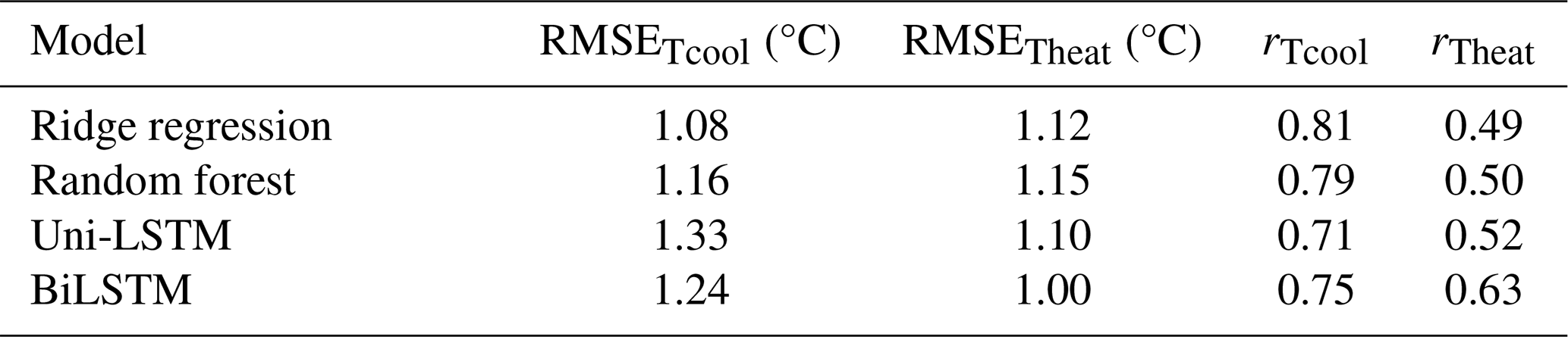
Note: Values are pooled out-of-fold predictions from three-fold cross-validation and are not directly comparable to the final-model performance in Sect. 3.1. RMSE_Tcool and RMSE_Theat are the root mean squared errors (°C) of the out-of-fold predictions of the cooling and heating base temperatures, respectively. r_Tcool and r_Theat are Pearson correlations between the predicted and labeled cooling and heating base temperatures, respectively.

3.2 Global Tbase analysis

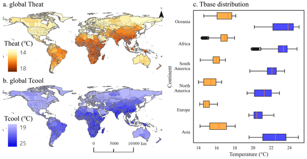
Global Tbase mapping reveals regionally differentiated temperature-dependent energy demand responses. Globally, Tcool ranges from 19 to 25 °C, with a mean of 22 °C and a median of 21.94 °C, while Theat ranges from 14 to 18 °C, with a mean of 16 °C and a median of 15.87 °C, which is consistent with physical logic (Fig. 2a and b).

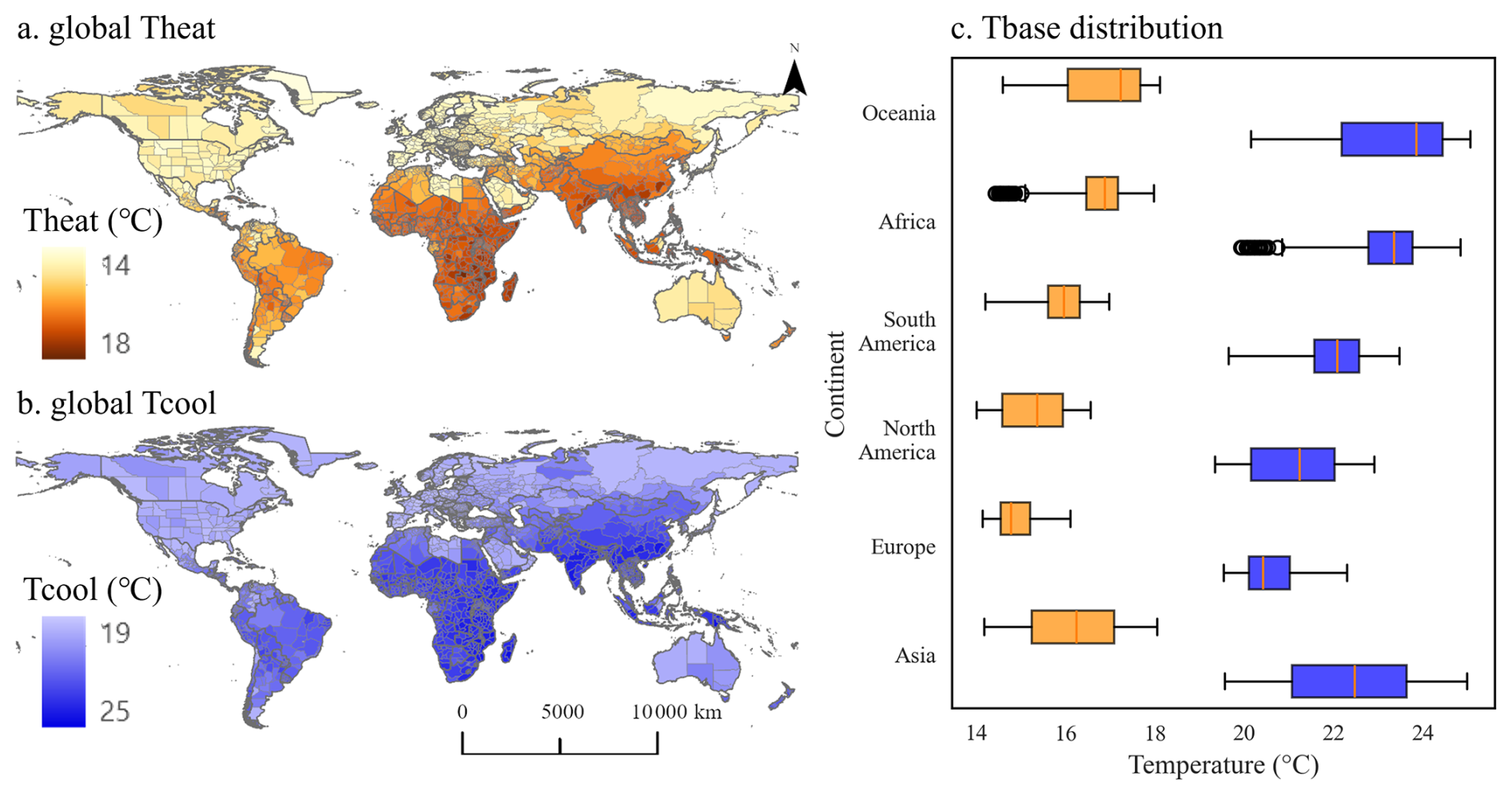
Figure 2 Global mapping of predicted base temperatures (Tcool and Theat) from the BiLSTM framework. (a, b) Geographic distribution of predicted heating and cooling base temperatures. (c) Box plots of the same predictions grouped by continent. Box plots show the median, interquartile range, and whiskers (1.5×IQR); points beyond the whiskers are outliers. Values are provided for all regions, including those where local temperatures currently do not cross a threshold and thus have no present-day cooling or heating demand; whether such demand occurs depends on local temperature evolution and population distribution, and may change under future climate warming.

The Tcool and Theat present a generally consistent distribution pattern, characterized by lower Tbase values in high-latitude regions and higher values in low-latitude regions (Fig. 2c). North America and Europe, which are predominantly composed of developed countries, have the lowest median Tcool and Theat. These patterns are consistent with prior findings that higher-income populations may use cooling at lower outdoor temperatures (Cong et al., 2022), and that well-insulated building stocks are associated with lower heating thresholds. However, Libya, Gabon, Algeria, Botswana, and South Africa in the African region have relatively low Theat, indicating within-continent heterogeneity that the dataset is able to capture. Asia spans the longest latitudinal range and exhibits the largest inter-regional economic disparities, resulting in the widest distribution of Tbase values (Tcool: 19.57–24.99 °C, Theat: 14.18–18.05 °C). Southern China and India have higher Tbase values. A base temperature test for India based on the energy signature method showed that the median Theat in many regions is 17.4 °C (Bhatnagar et al., 2018), which closely aligns with the median Theat of 17.05 °C found in this study. Oceania's Tbase is more dispersed, which is due to the smallest number of regions included. Differentiated Tbase can support energy-saving planning, building renovation, and climate-adaptive design.

Figure 3 Workflow for technical validation.

3.3 Technical validation

To further demonstrate the effectiveness of the predicted Tbase, a comprehensive validation framework is employed, as shown in Fig. 3. In this framework, energy demand datasets from 16 regions are employed to perform external validations of Tbase (Table A3). These datasets cover major continents globally, with relatively uniform distribution to ensure the comprehensiveness and representativeness of the validation results.

Three validation approaches are employed to assess whether predicted Tbase improves the accuracy of temperature-dependent energy demand modelling, including direct validation, indirect validation and sensitivity analysis (Fig. 3). Direct validation applies the segmented linear regression method described earlier to determine Tbase for each dataset, and then compares these results with the predicted values to validate the accuracy and reliability of the prediction results in practical applications. Indirect validation uses both the predicted Tbase and reference values from literature or official sources to forecast building energy demand through degree-day modelling. For each energy dataset, the following indirect validation procedure is adopted to evaluate the accuracy of the predicted Tbase. First, based on the corresponding temperature data, two sets of degree days are calculated: (1) HDD and CDD calculated using the predicted Tbase from this study; (2) HDD and CDD calculated using reference Tbase values from literature or official sources. Subsequently, statistical analyses are performed on the above two sets of degree days with actual energy consumption data, including: (1) correlation analysis, calculating the time-series correlation coefficient (TCC) to quantify the linear relationship between degree days and energy consumption. The TCC is computed as the cross-correlation between the two series; at zero time lag it is equivalent to the Pearson correlation coefficient, and the zero-lag value is adopted here. (2) regression analysis, establishing degree day-energy consumption regression models and calculating root mean square error (RMSE) to evaluate prediction accuracy. Finally, the modelling performance of the predicted Tbase is evaluated through comparative analysis. If the HDD and CDD calculated based on the predicted Tbase exhibit higher correlation coefficients with actual energy consumption and the corresponding regression models have lower RMSE, this indicates superior accuracy. For sensitivity analysis, the TCC is used to analyse how changes in Tbase affect the correlation between energy demand and HDD or CDD, thereby evaluating the performance of the predicted Tbase.

For the 16 energy demand datasets at the regional and building levels, the validation results are summarized in Table 3. Both direct and indirect validation results show that the predicted Tbase performs well across most datasets. Direct validation yields average errors of 0.68 °C for Tcool and 1.08 °C for Theat across the 16 datasets. Indirect validation demonstrates that the predicted Tbase substantially improves the accuracy of building energy demand modelling in two key aspects. First, the TCC between energy demand and HDD/CDD calculated using the predicted Tbase is greater than or equal to that obtained using reference Tbase values. This indicates that predicted Tbase maintains or enhances the explanatory power of temperature-dependent energy demand variations. On average, the predicted Tbase improves TCC across the validation datasets from 0.67 to 0.81. Second, the predicted Tbase substantially reduces the RMSE of both cooling and heating energy demand modelling. Specifically, the RMSE of cooling and heating energy demand modelling decreases by comparable margins, averaging approximately 10 % in both cases.

Table 3 Summaries of validation.

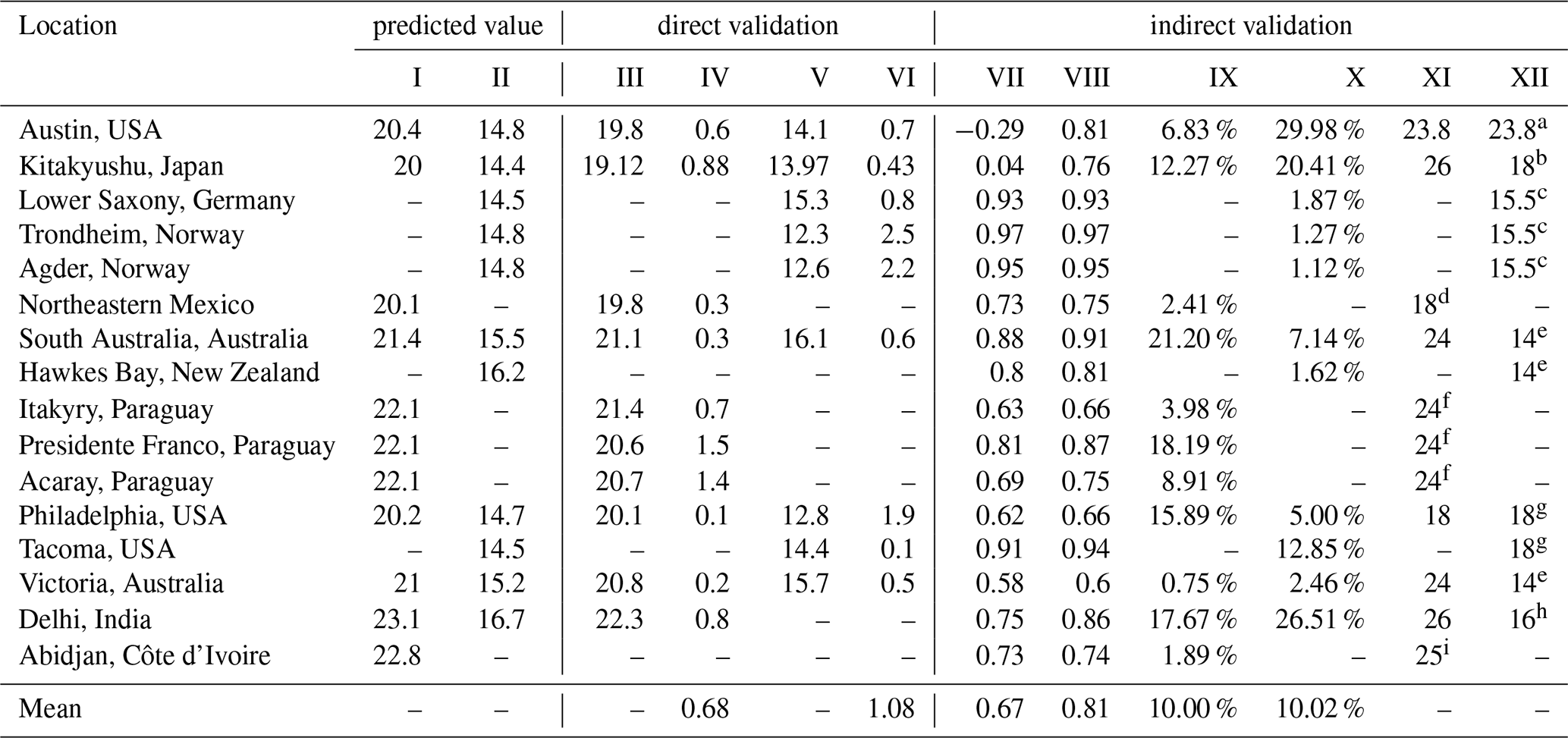
Note 1: I: predicted Tcool from BiLSTM framework; II: predicted Theat from BiLSTM framework; III: Tcool from segmented linear regression method; IV: Absolute error of Tcool; V: Theat from segmented linear regression method; VI: Absolute error of Theat; VII: TCC based on reference Tbase; VIII: TCC based on predicted Tbase; IX: decreased RMSE for CDD-energy demand modelling by predicted Tcool; X: decreased RMSE for HDD-energy demand modelling by predicted Theat; XI: reference Tcool; XII: reference Theat.
Note 2: ^a Feng et al., 2021; ^b Yuan et al., 2024; ^c Filahi et al., 2024; ^d Corrales-Suastegui et al., 2021; ^e Livada et al., 2021; ^f Kennard et al., 2022; ^g ASHRAE, 2009; ^h Borah et al., 2015; ⁱ Dicko et al., 2024.

The sensitivity analysis evaluates the proximity of the TCC value derived from the predicted Tbase to the maximum achievable TCC value. A TCC value approaching the maximum indicates higher accuracy of the predicted Tbase and enhanced performance in temperature-dependent energy demand modelling. Figures A2–A15 demonstrate that across all datasets, the TCC values calculated using the predicted Tbase approximate their respective maxima, confirming the effectiveness of the predicted Tbase parameters in HDD/CDD-based modelling. Although three datasets show prediction errors greater than 2 °C, the indirect validation results indicate that predicted Tbase still contributes to enhanced energy demand modelling accuracy, as evidenced by consistent RMSE reductions in all instances. Overall, the predicted Tbase improves the ability to explain and model temperature-dependent energy demand variations.

3.3.1 Building-level validation

In order to present the validation process more clearly, the detailed results of a building-level dataset and a regional-level dataset are presented below. Figure 4 shows the validation results of a residential building in South Australia, Australia (Sharma et al., 2019). Direct validation shows absolute prediction errors of 0.3 °C between the predicted Tcool (21.4 °C) and the actual value (21.10 °C), and 0.6 °C between the predicted Theat (15.5 °C) and the actual value (16.10 °C) (Fig. 4a). Figure 4b demonstrates that the TCCs corresponding to Tcool and Theat approach their respective maximum values across the tested base temperature range, implying that the predicted Tbase effectively captures temperature-dependent energy demand variations. Following previous studies, 14 and 24 °C are adopted as reference base temperatures for this dataset (Livada et al., 2021), and indirect validation is performed to compare the reliability of predicted versus reference Tbase values in residential energy demand modelling. The TCC calculated using predicted Tbase (15.5 °C/21.4 °C) reaches 0.91, exceeding the TCC based on the reference Tbase (14 °C/24 °C) of 0.88, representing a modest improvement of 0.03 (Fig. 4c). For heating energy demand modelling, RMSE decreases from 1.82 to 1.69 kWh, achieving a relative improvement of 7.14 % (Fig. 4d and f). For cooling energy modelling, RMSE is reduced from 1.84 to 1.45 kWh, corresponding to a relative improvement of 21.20 % (Fig. 4e and g). These results indicate that energy demand modelling based on predicted Tbase is more reliable.

Figure 4 Visualization of CDD and HDD versus energy consumption at different base temperatures of a building in South Australia, Australia. (a) Direct validation of Tcool and Theat; (b) TCC versus base temperature; (c) indirect validation (TCC, predicted vs. reference Tbase); (d–g) heating and cooling energy demand modelling and RMSE using predicted versus reference base temperatures.

Figure 5 Visualization of HDD versus energy consumption at different base temperatures in Tacoma, USA. (a) Direct validation of Theat; (b) TCC versus base temperature; (c) indirect validation (TCC, predicted vs. reference Tbase); (d, e) heating energy demand modelling and RMSE using predicted versus reference base temperatures.

3.3.2 Region-level validation

For the regional-level energy demand dataset, Fig. 5 presents the validation results of daily energy demand modelling in Tacoma, USA. To extract residential energy demand from the raw dataset, the residential sector's share of annual end-use energy demand from the U.S. Energy Information Administration (EIA) (https://www.eia.gov/, last access: 1 December 2024) has been applied to daily total energy consumption data to derive daily residential energy demand. The direct validation results suggest that this area has significant heating demand, with an error of only 0.1 °C between the predicted Theat (14.5 °C) and the actual value (14.4 °C) (Fig. 5a). Figure 5b shows that the TCC corresponding to Theat is very close to its maximum value, demonstrating that the predicted Tbase effectively captures residential energy demand variations. The official value of 18 °C is adopted as the reference Tbase for residential energy demand modelling in this dataset. The TCC calculated using the predicted Tbase (14.5 °C) reaches 0.94, exceeding the TCC based on the reference Tbase (18 °C) of 0.91 (Fig. 5c) (ASHRAE, 2009). The RMSE is reduced from 172.65 to 150.46 MWh, corresponding to a relative improvement of 12.85 % (Fig. 5d and e). These results demonstrate that the predicted base temperatures have good applicability in regional-scale energy demand modelling.

3.4 Potential application of the Tbase dataset

Efforts to enhance degree-day models persist in order to improve efficiency and accuracy in building energy modelling. Numerous studies have calculated region-specific Tbase across Europe, Africa, India, and globally (Wenz et al., 2017; Bhatnagar et al., 2018; Staffell et al., 2023), significantly improving the accuracy of regional building energy demand modelling. However, the heavy reliance on actual building energy demand datasets constrains the extension of Tbase estimation to broader detailed spatial scales. This study addresses this limitation through a machine learning approach.

The Tbase dataset developed in this study has significant potential for use in a wide range of areas related to degree-day modelling. Firstly, applying Tbase to heating and cooling energy demand modelling on a consistent global scope can provide scientific support for differentiated energy system planning and climate adaptation strategies in building design. Secondly, Tbase can be used for a wide range of heat exposure assessments, contributing to studies on the health dimensions of climate change impacts and providing data to support strategies for heatwave warning and the protection of vulnerable populations (Broomandi et al., 2025; Hu et al., 2025). Finally, Tbase holds significant value in large-scale model coupling. Integration of the Tbase datasets into various Earth System Models (e.g., CESM) and Integrated Assessment Models (e.g., GCAM, IMAGE) could help reduce long-term modelling uncertainties. In turn, incorporating these more accurate representations of energy demand modelling results into energy-economic models can provide a reliable modelling framework for designing decarbonization pathways.

3.5 Limitations and uncertainties of the Tbase dataset

Limitations and uncertainties related to the research design and model are discussed below. Firstly, the dataset's reliance on electricity and natural gas consumption statistics inadequately captures heating demand from alternative energy sources. Especially in energy-poor regions, the decentralized nature of heating makes it difficult to account for the use of polluting sources, such as coal and diesel (Burguillo and Juez-Martel, 2024; Kozarcanin et al., 2019). This limitation in data acquisition makes it difficult to accurately characterize heating demand patterns across time and temperature. Secondly, given the unavailability of extensive data, building characteristics such as type, age, floor area, insulation performance, number of floors, and other attributes are not differentiated in this study. The Tbase dataset, therefore, provides generalized energy demand estimates rather than building-type-specific predictions. In addition, the dynamic changes in Tbase were not taken into account due to the limitations of acquiring extensive long-term energy consumption data.

To assess how choices in the label-generation process affect the dataset, we tested the sensitivity to the goodness-of-fit threshold of the segmented regression. Relaxing the inclusion criterion from R²>0.5 to 0.4 and tightening it to 0.6 changed the number of retained units between 123 and 149, while the overall label distribution remained essentially unchanged: mean Theat ranged over 14.47–14.67 °C (range 0.2 °C) and mean Tcool over 20.66–21.49 °C (range 0.83 °C), both smaller than the model uncertainty interval. This indicates that the dataset is insensitive to the fitting threshold. In addition, Theat estimated with a UKMO-based alternative breakpoint method over 20 UK regions differs from that from Eq. (1) by only 0.83 °C on average (Appendix A), further suggesting limited dependence on the breakpoint-selection approach.

Beyond the label-generation process examined above, uncertainty in the Tbase results also arises from the model itself. This can be decomposed into aleatoric (data noise) and epistemic (model knowledge) uncertainty (Xu et al., 2025; He et al., 2025a). The epistemic uncertainty of the Tbase dataset was estimated by 30 data sampling analyses using MC Dropout for meteorological, socioeconomic, and geographic background data collected for 3385 spatial units. The MC Dropout employs a neural disconnection mechanism based on randomness to evaluate network sensitivity to model variations (Xu et al., 2025). This approach is widely used for uncertainty quantification due to its computational simplicity and efficiency. Uncertainty was quantified by calculating the standard deviation (std) across the results of multiple analyses, where larger values indicate greater uncertainty in Tbase estimates due to model variability or limited data. The results are shown in Fig. 6. The uncertainty ranges for Theat and Tcool are [0.56,1.61] and [0.82,2.26] °C, respectively. Although Theat shows lower model accuracy, its target distribution is more concentrated (the interquartile range, IQR, is narrower, see Fig. 1d), resulting in a smaller uncertainty interval. By focusing on the maximum uncertainty and normalizing by their respective mean values (22 °C for Tcool, 16 °C for Theat), both variables exhibit comparable relative uncertainties of approximately 10 %, indicating consistent uncertainty quantification across different targets. The spatial distribution of std shows that the uncertainty is at a medium-low level in most regions, such as North America, Europe, northern Asia, and Oceania. The training samples in Africa, South America, and western Asia are sparse, and the std is relatively high. In the future, further increasing the sample size in sparsely sampled regions will reduce the epistemic uncertainty of the model.

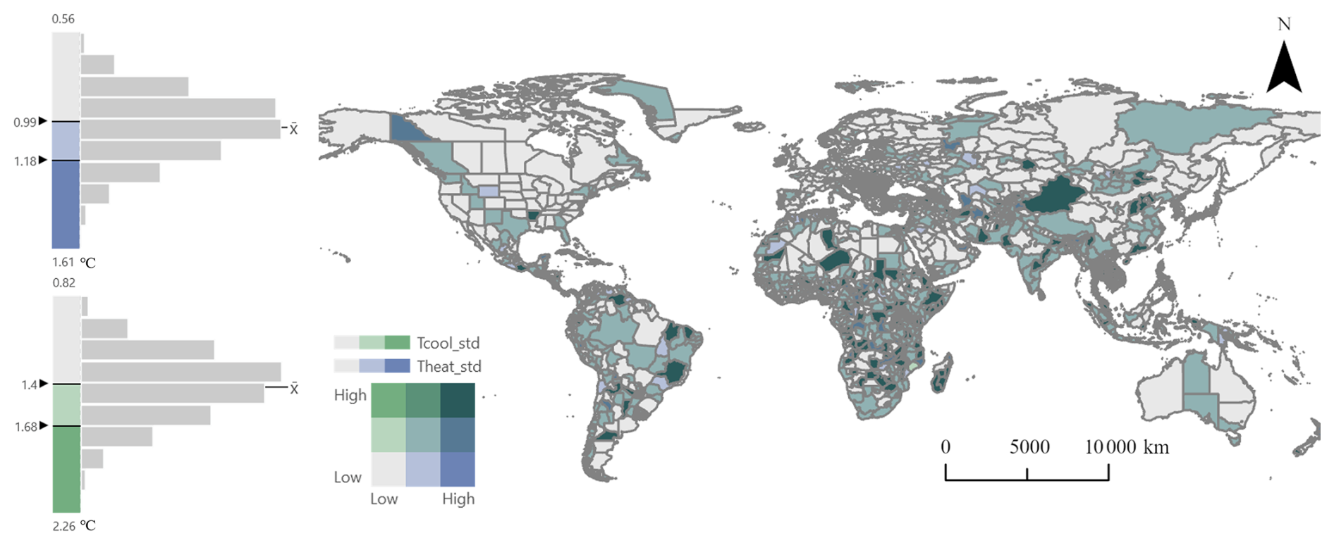
Figure 6 Tbase uncertainty analysis based on the limitations in the model.

The representativeness of the training sample also affects the reliability of the global extrapolation. The 131 training units span 24 countries and are mainly concentrated in temperate, mid-to-high-latitude regions. This distribution covers the climatic and socioeconomic conditions of most inhabited areas reasonably well, while tropical, arid, and Southern-Hemisphere regions are covered more sparsely. The MC Dropout analysis above quantifies model uncertainty, whereas limited spatial coverage introduces an additional, extrapolation-related uncertainty; the two compound in sparsely trained regions, consistent with the higher standard deviations found over Africa, South America, and western Asia in the MC Dropout results. Therefore, users are encouraged to consult the accompanying uncertainty layer when interpreting results for these regions, and expanding the training sample there in the future would further improve representativeness.

4 Data availability

The proposed global Tbase dataset can be acquired from https://doi.org/10.6084/m9.figshare.30646376.v2 (He et al., 2025b).

5 Conclusion

This study developed a global regional-scale Tbase dataset, including both Tcool and Theat, by integrating comprehensive energy demand, meteorological, and socioeconomic data using a BiLSTM framework with an attention mechanism. The Tbase values varied across regions worldwide, with Tcool ranging from 19 to 25 °C (mean: 22 °C; median: 21.94 °C), and Theat ranging from 14 to 18 °C (mean: 16 °C; median: 15.87 °C). Compared to the use of a fixed Tbase, these heterogeneous values better capture local climate characteristics, socioeconomic conditions, and energy use behaviours. The Tbase is primarily applicable to general building energy demand modelling for assessing energy requirements to achieve universal thermal comfort.

The model construction incorporates several strategies to minimize the impact of small samples. First, stratified sampling based on geographic clustering ensures representative distribution between the training and test sets. Second, joint training of Tcool and Theat using an adaptive MSE-based loss function maximizes data utilization. Third, the attention mechanism captures critical temporal patterns to enhance training efficiency. Based on 131 regions (with 80 % used for training and 20 % for testing), internal validation shows RMSE values of 1.39 °C (training) and 1.33 °C (testing), with correlation coefficients of 0.84 for Tcool and 0.70 for Theat, demonstrating good generalization performance.

External validation using 16 independent building energy demand datasets from various global regions (completely separate from the 131 regions used in the model construction phase) demonstrates that predicted Tbase consistently improves the accuracy of energy demand modelling. The average prediction errors for Tcool and Theat are 0.68 and 1.08 °C, respectively. Compared with official or empirical Tbase values, the predicted Tbase increases the average TCC between energy demand and CDD/HDD from 0.67 to 0.81 and reduces RMSE by comparable margins of approximately 10 % for cooling and heating. Uncertainty analysis revealed epistemic uncertainties of 0.56–2.26 °C, with the highest values confined to sparsely sampled regions, indicating that most regions are reliable while sparsely trained areas carry higher uncertainty. These results underscore the model's ability to effectively capture regional heterogeneity in temperature-dependent energy demand responses.

The resulting dataset supports a wide range of regional-scale applications and increases research productivity across multiple domains. Most significantly, it improves the accuracy of degree-day energy demand models, enabling the exploration of how adjustments to temperature thresholds affect energy requirements. Additionally, the dataset facilitates climate change impact assessments, such as accurate heat exposure analysis. Finally, coupling the Tbase dataset with Earth system models and integrated assessment models has the potential to reduce uncertainty in climate-energy interactions, thereby enhancing long-term energy modelling performance. Overall, this spatially continuous Tbase dataset helps address key limitations in building energy modelling and opens new research opportunities in climate-responsive energy planning.

Appendix A: Cross-method validation of base temperatures against a UKMO-based approach

To assess our base-temperature estimates against an independent, max/min–based method in a European context, we compared the heating base temperature from Eq. (1) with that obtained from a UK Met Office (UKMO) degree-day formulation combined with a performance-line fit (Deroubaix et al., 2021; CIBSE, 2006; Spinoni et al., 2018). The HDD under the UKMO method is computed from the daily minimum, mean, and maximum temperatures (T_min, T_mean, T_max) relative to a Theat:

$$\begin{array}{}\text{(A1)}& \mathrm{\text{HDD}}=\left\{\begin{array}{ll}\mathrm{0},& T_{\text{heat}}\le T_{\text{min}}\\ \frac{T_{\text{heat}}-T_{\text{min}}}{\mathrm{4}},& T_{\text{min}}<T_{\text{heat}}<T_{\text{mean}}\\ \frac{T_{\text{heat}}-T_{\text{min}}}{\mathrm{2}}-\frac{T_{\text{max}}-T_{\text{heat}}}{\mathrm{4}},& T_{\text{mean}}\le T_{\text{heat}}<T_{\text{max}}\\ T_{\text{heat}}-T_{\text{mean}},& T_{\text{heat}}\ge T_{\text{max}}\end{array}\right..\end{array}$$

The base temperatures from Eq. (1) agree closely with those from an independent UKMO-based method, indicating that our estimates are robust to the choice of estimation formulation. For each region we scanned candidate base temperatures from 10 to 18 °C in 0.25 °C steps. At each candidate Theat we computed the daily HDD series and regressed daily energy demand on HDD; candidates yielding a non-positive slope were discarded. The Theat giving the highest R² was taken as the UKMO-based heating base temperature (Theat, UKMO). To keep the comparison fair, energy demand was cleaned using the same procedure applied to Eq. (1). The comparison used the 20 UK regions with the most complete daily energy records. Across these regions, the two methods agree closely (mean absolute difference 0.83 °C, RMSE 0.87 °C, Pearson r=0.83), with Eq. (1) giving slightly lower values. As shown in Fig. A1, the R² profiles are broadly flat near their maxima, so this offset corresponds to a negligible difference in goodness-of-fit; the two methods are therefore effectively equivalent in how well they explain the observed energy–temperature relationship.

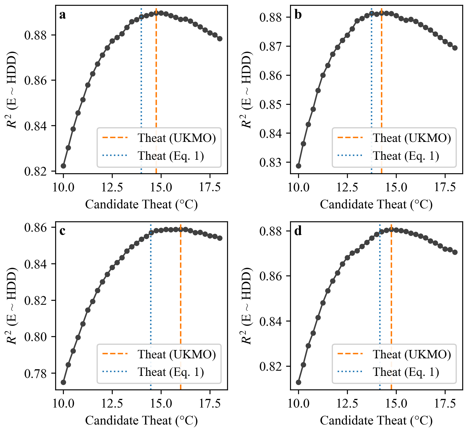
Figure A1 R²(E ∼ HDD) as a function of candidate heating base temperature for four representative UK regions, selected by the median (a), minimum (b), maximum (c), and near-mean (d) difference between the two methods. Dashed line: Theat from the UKMO performance line (R² maximum); dotted line: Theat from Eq. (1).

Table A1 Details of the energy datasets used for calculating the target Tbase.

Table A2 Tcool and Theat values used for model training.

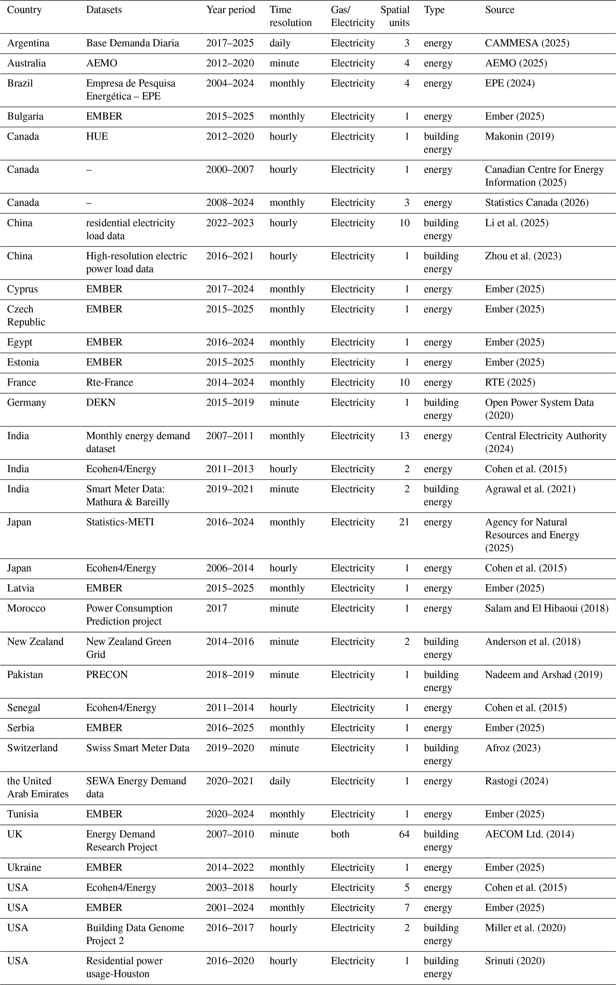
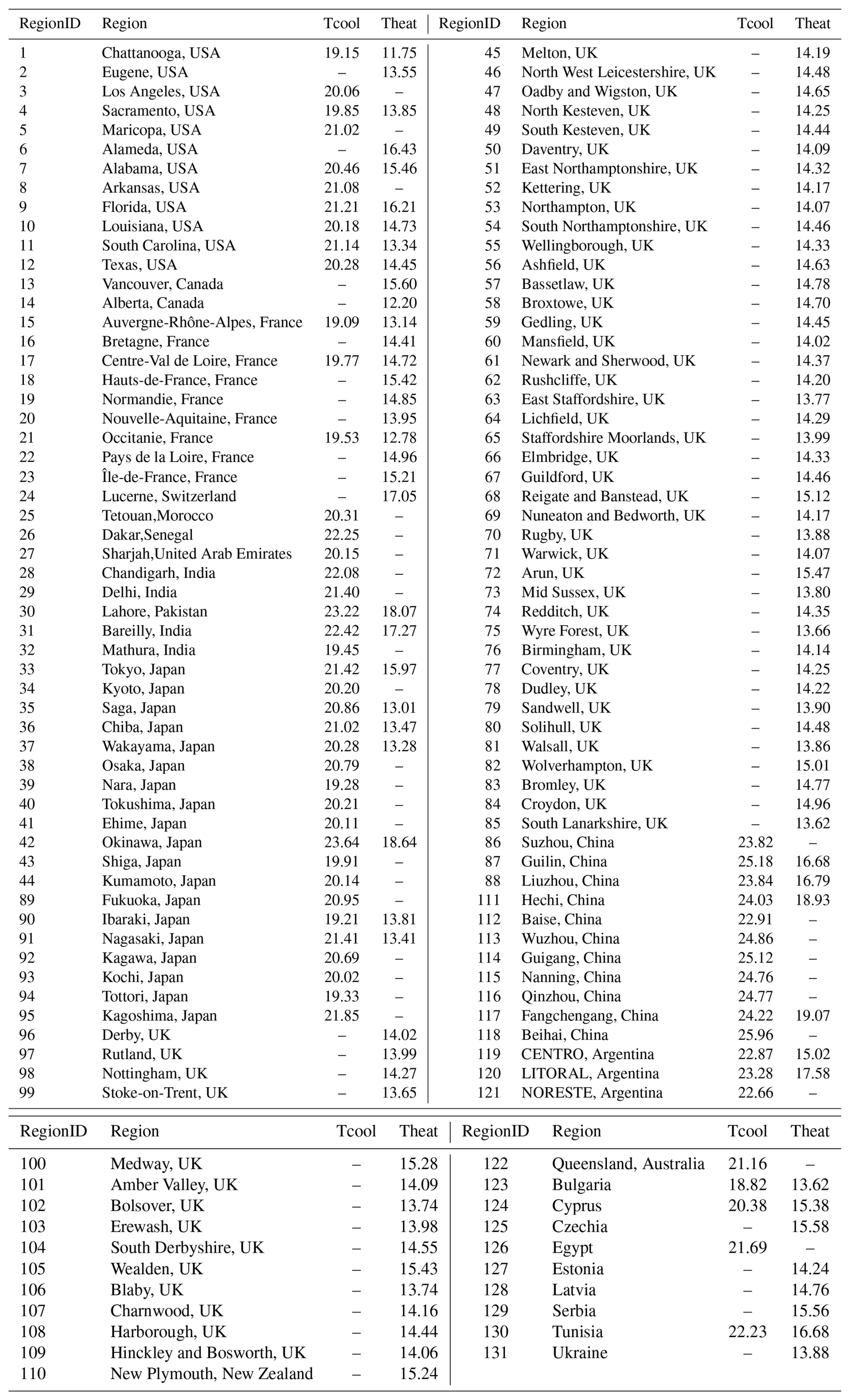
Table A3 Details of 16 energy demand datasets used for external validation.

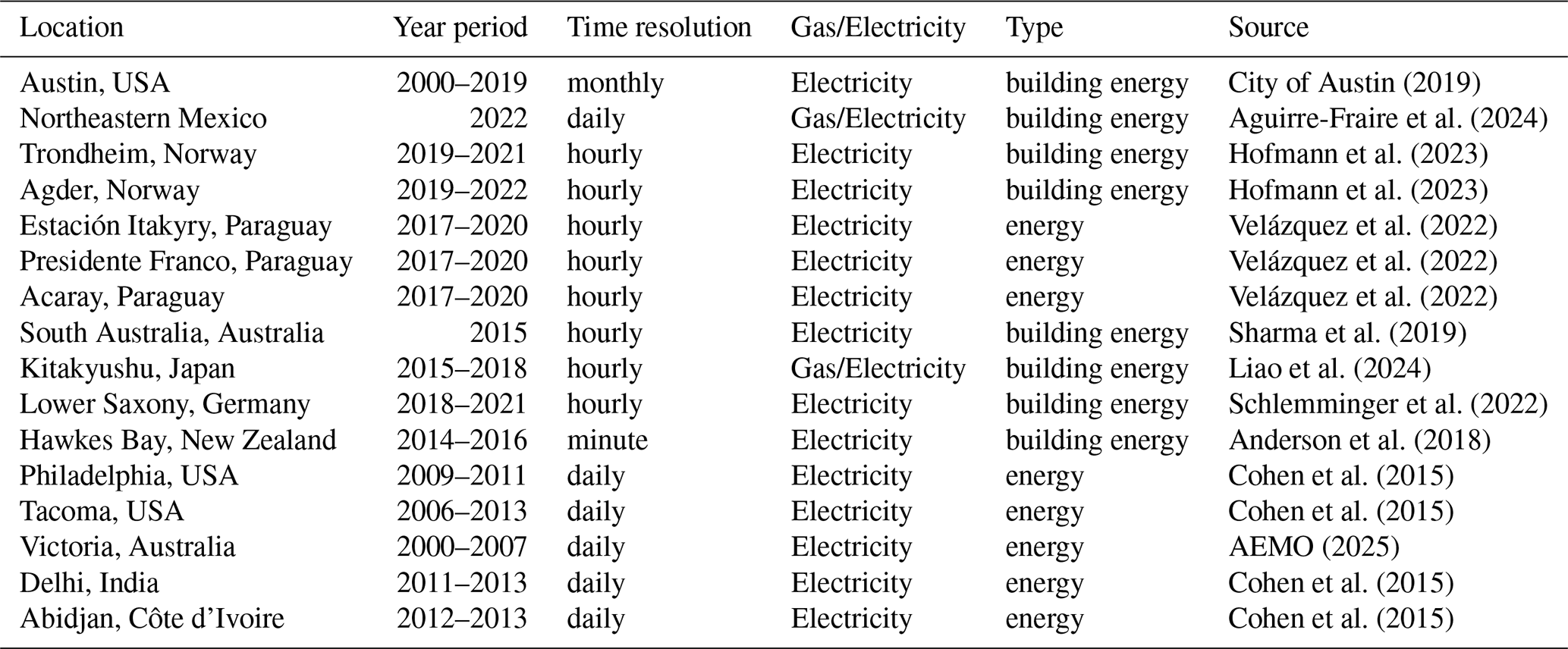
Figure A2 Visualization of HDD and CDD versus energy consumption at different base temperatures in Austin, USA. (a) Direct validation of Tcool and Theat; (b) TCC versus base temperature; (c) indirect validation (TCC, predicted vs. reference Tbase); (d–g) heating and cooling energy demand modelling and RMSE using predicted versus reference base temperatures.

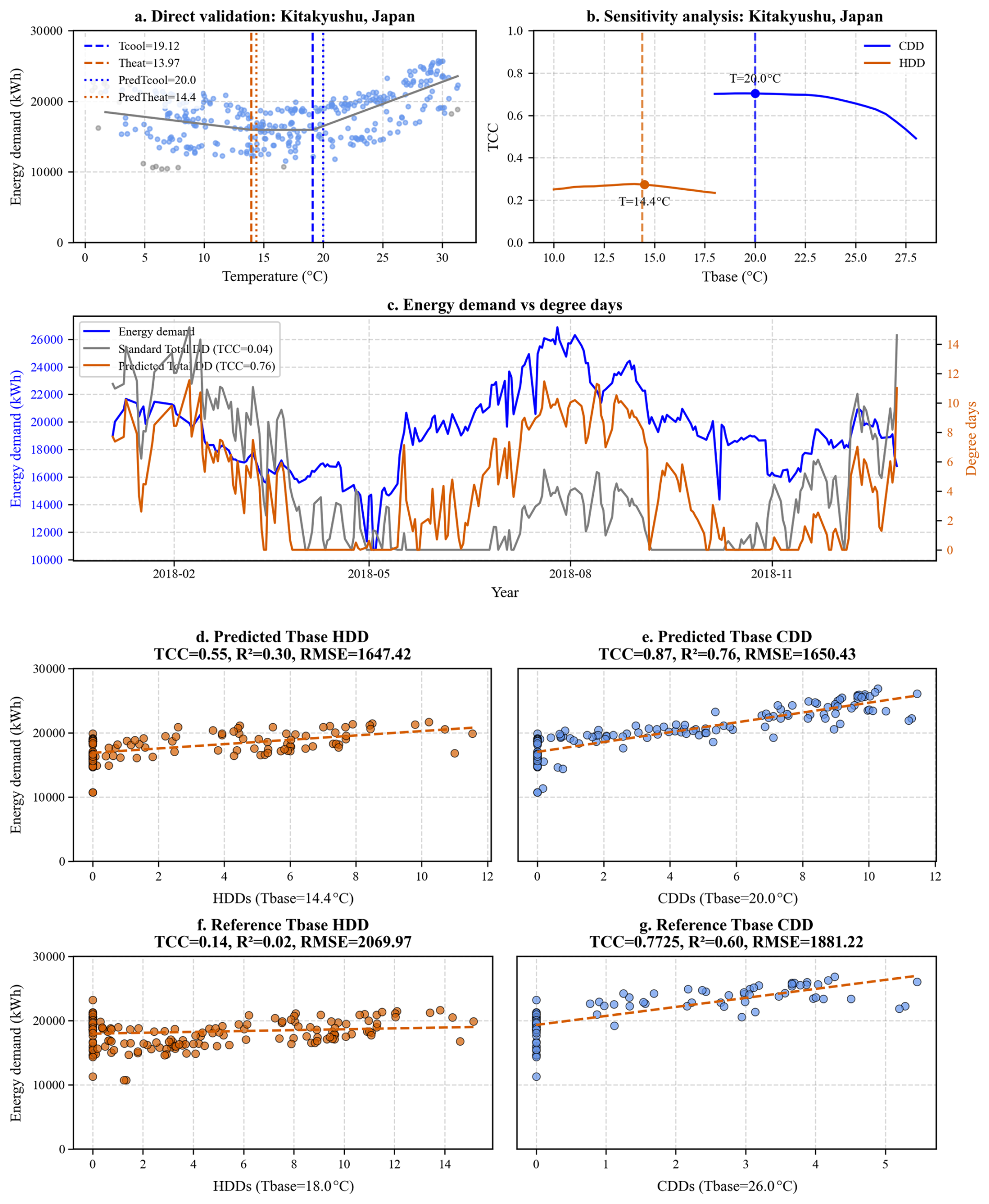
Figure A3 Visualization of HDD and CDD versus energy consumption at different base temperatures in Kitakyushu, Japan. (a) Direct validation of Tcool and Theat; (b) TCC versus base temperature; (c) indirect validation (TCC, predicted vs. reference Tbase); (d–g) heating and cooling energy demand modelling and RMSE using predicted versus reference base temperatures.

Figure A4 Visualization of HDD versus energy consumption at different base temperatures in Lower Saxony, Germany. (a) Direct validation of Theat; (b) TCC versus base temperature; (c) indirect validation (TCC, predicted vs. reference Tbase); (d, e) heating energy demand modelling and RMSE using predicted versus reference base temperatures.

Figure A5 Visualization of HDD versus energy consumption at different base temperatures in Trondheim, Norway. (a) Direct validation of Theat; (b) TCC versus base temperature; (c) indirect validation (TCC, predicted vs. reference Tbase); (d, e) heating energy demand modelling and RMSE using predicted versus reference base temperatures.

Figure A6 Visualization of HDD versus energy consumption at different base temperatures in Agder, Norway. (a) Direct validation of Theat; (b) TCC versus base temperature; (c) indirect validation (TCC, predicted vs. reference Tbase); (d, e) heating energy demand modelling and RMSE using predicted versus reference base temperatures.

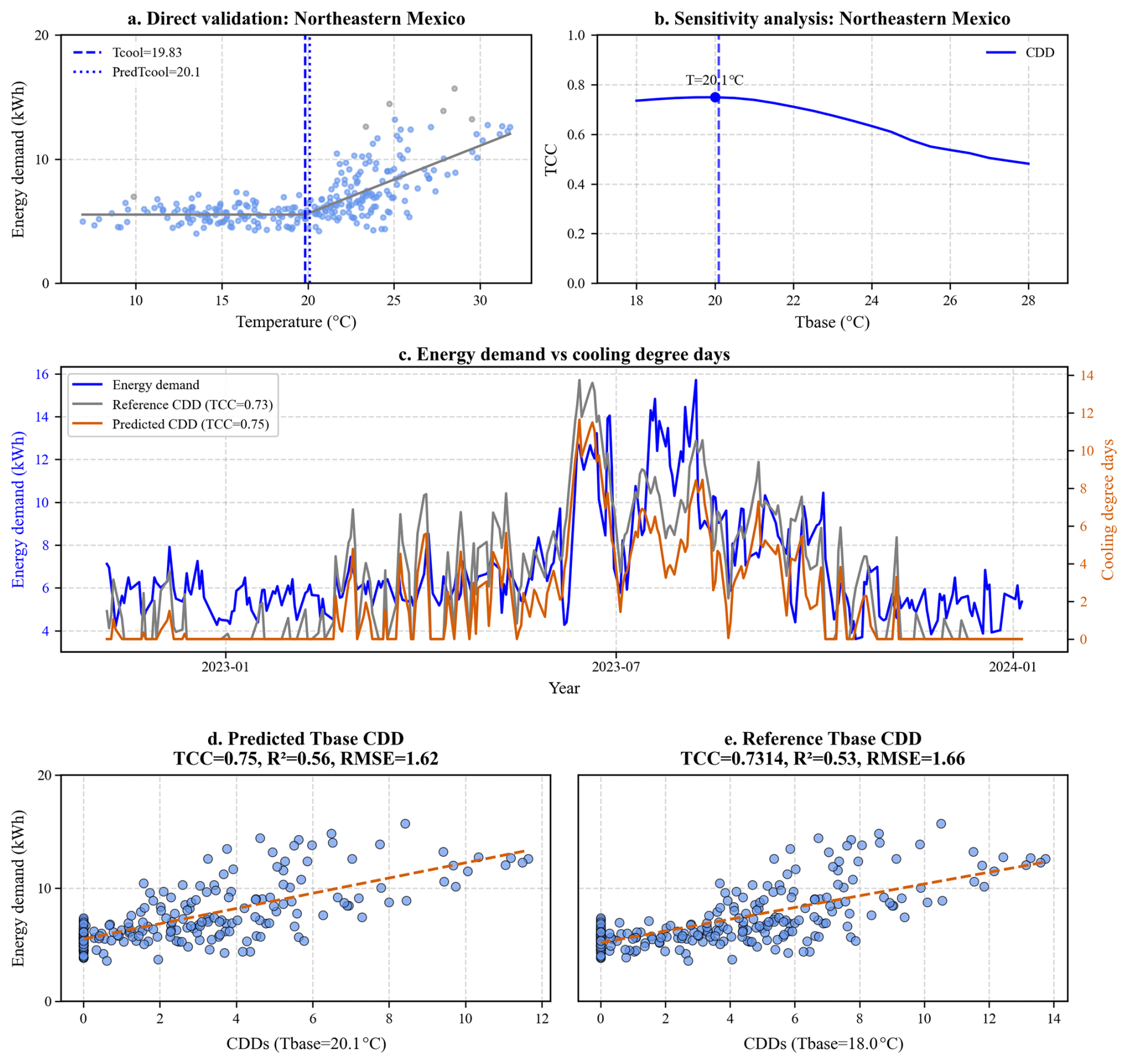
Figure A7 Visualization of CDD versus energy consumption at different base temperatures in Northeastern Mexico. (a) Direct validation of Tcool; (b) TCC versus base temperature; (c) indirect validation (TCC, predicted vs. reference Tbase); (d, e) cooling energy demand modelling and RMSE using predicted versus reference base temperatures.

Figure A8 Visualization of HDD versus energy consumption at different base temperatures in Hawkes Bay, New Zealand. (a) Direct validation of Theat; (b) TCC versus base temperature; (c) indirect validation (TCC, predicted vs. reference Tbase); (d, e) heating energy demand modelling and RMSE using predicted versus reference base temperatures.

Figure A9 Visualization of CDD versus energy consumption at different base temperatures in Itakyry, Paraguay. (a) Direct validation of Tcool; (b) TCC versus base temperature; (c) indirect validation (TCC, predicted vs. reference Tbase); (d, e) cooling energy demand modelling and RMSE using predicted versus reference base temperatures.

Figure A10 Visualization of CDD versus energy consumption at different base temperatures in Presidente Franco, Paraguay. (a) Direct validation of Tcool; (b) TCC versus base temperature; (c) indirect validation (TCC, predicted vs. reference Tbase); (d, e) cooling energy demand modelling and RMSE using predicted versus reference base temperatures.

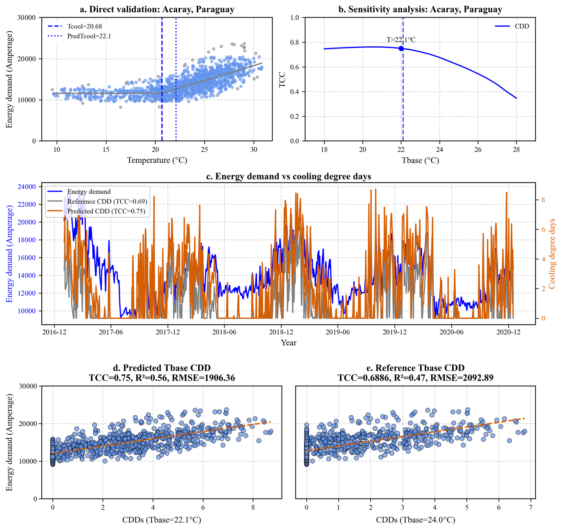
Figure A11 Visualization of CDD versus energy consumption at different base temperatures in Acaray, Paraguay. (a) Direct validation of Tcool; (b) TCC versus base temperature; (c) indirect validation (TCC, predicted vs. reference Tbase); (d, e) cooling energy demand modelling and RMSE using predicted versus reference base temperatures.

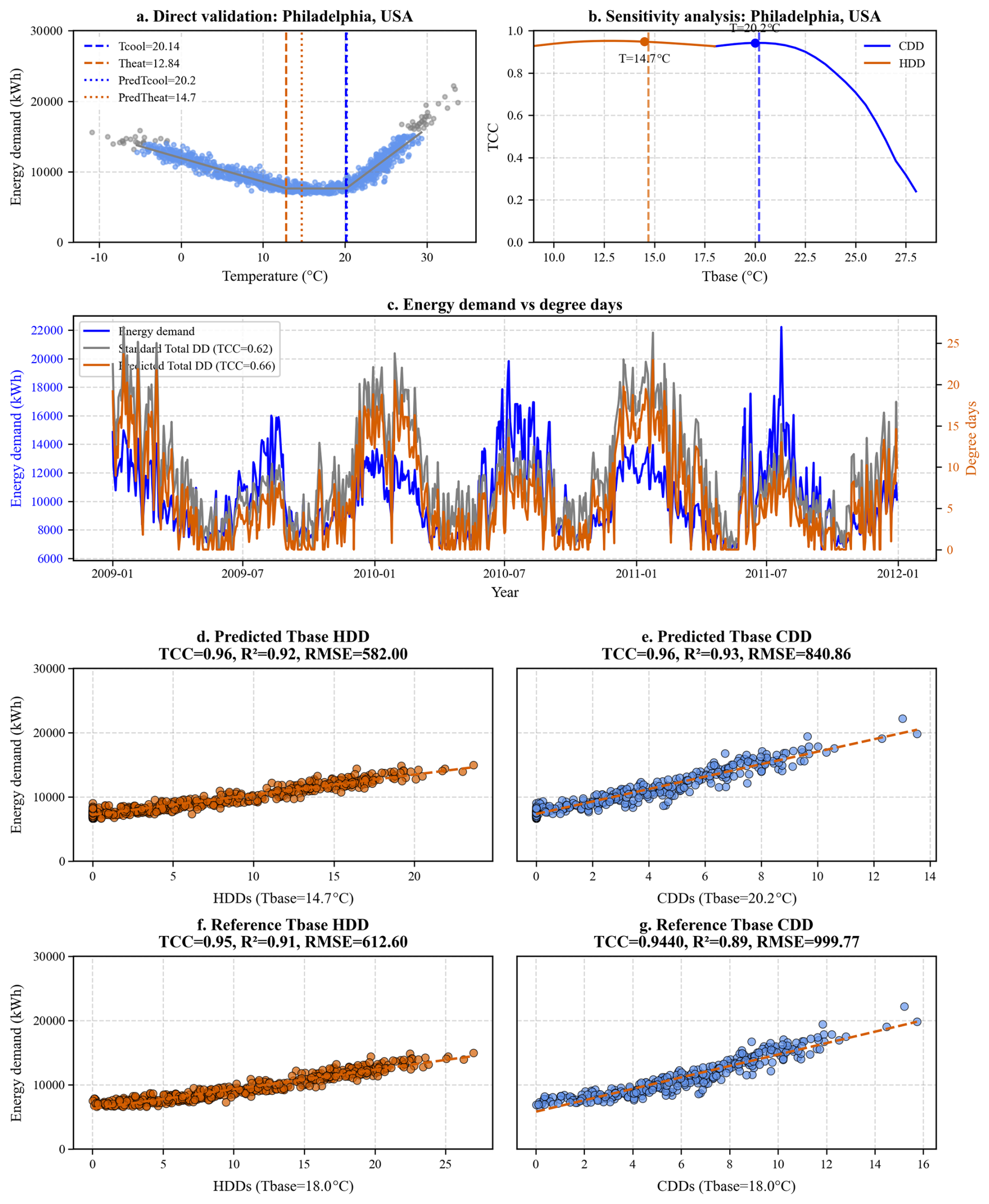
Figure A12 Visualization of HDD and CDD versus energy consumption at different base temperatures in Philadelphia, USA. (a) Direct validation of Tcool and Theat; (b) TCC versus base temperature; (c) indirect validation (TCC, predicted vs. reference Tbase); (d–g) heating and cooling energy demand modelling and RMSE using predicted versus reference base temperatures.

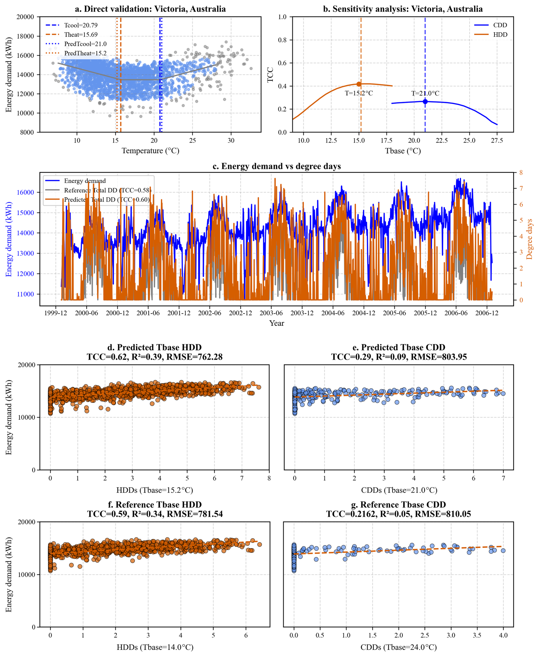
Figure A13 Visualization of HDD and CDD versus energy consumption at different base temperatures in Victoria, Australia. (a) Direct validation of Tcool and Theat; (b) TCC versus base temperature; (c) indirect validation (TCC, predicted vs. reference Tbase); (d–g) heating and cooling energy demand modelling and RMSE using predicted versus reference base temperatures.

Figure A14 Visualization of HDD and CDD versus energy consumption at different base temperatures in Delhi, India. (a) Direct validation of Tcool and Theat; (b) TCC versus base temperature; (c) indirect validation (TCC, predicted vs. reference Tbase); (d–g) heating and cooling energy demand modelling and RMSE using predicted versus reference base temperatures.

Figure A15 Visualization of CDD versus energy consumption at different base temperatures in Abidjan, Cote D'Ivoire. (a) Direct validation of Tcool; (b) TCC versus base temperature; (c) indirect validation (TCC, predicted vs. reference Tbase); (d, e) cooling energy demand modelling and RMSE using predicted versus reference base temperatures.