HyBEAR: a hyperspectral benchmark for bare soil detection

Detecting bare soil areas is an important step in the analysis of Earth observation data in a variety of Precision Agriculture (PA) applications focused on quantifying soil properties and assessing soil quality. In this paper, we introduce the HyBEAR benchmark – a novel large-scale collection of high-resolution hyperspectral aerial images (with 2 m ground sampling distance) accompanied by manual bare soil annotations verified by domain experts. Usually, the bare soil detection problem is tackled at the pixel level, meaning that detection methods classify all pixels as either bare soil or background. In contrast to this approach, we provide pixel-level annotations for the entire agricultural parcels (if the parcel is labeled as bare soil, then all pixels within that parcel are labeled accordingly), and aim to support the development of methods that identify entire fields with no vegetation. Commonly, such fields undergo further analysis to determine specific soil parameters and characteristics that are important when planning various PA activities, such as fertilization. The HyBEAR benchmark includes (i) the largest-to-date (108 064 591 pixels, corresponding to 43 225 ha) and most heterogeneous dataset for bare soil detection, as well as (ii) the validation procedure (training-test splits and quality metrics) and a set of baseline results, obtained for a set of machine learning bare soil detection models. From the FULL collection of 1954 images in HyBEAR, which we divided into 5 spatially-disjoint folds, we additionally selected a random, stratified subset (MINI) of the images which may be useful for designing and verifying bare soil detection algorithms. Overall, HyBEAR is a step toward standardizing the way the community builds and confronts bare soil detection algorithms in a thorough, reproducible, and unbiased way. The dataset is publicly available at Zenodo: https://doi.org/10.5281/zenodo.17607897 (Wijata et al., 2025).

1 Introduction

Over the past decades, the agricultural sector has undergone significant transformations driven by human technological advancements aimed at meeting the escalating demands for food, fiber, and fuel from a rapidly expanding global population (Sishodia et al., 2020; Aijaz et al., 2025). With arable land becoming increasingly scarce, enhancing crop productivity has become crucial for ensuring food security (Pingali, 2012; Roy et al., 2024). Precision Agriculture (PA), emerging from technological advancements in fields such as Earth observation, data analytics, and in-situ field monitoring, plays a vital role in improving crop productivity. The global market for smart agriculture, which includes PA, was valued at approximately USD 15 billion in 2022 and is projected to grow to USD 30 billion by 2027 (Allied Market Research, 2023). This growth reflects the increasing adoption of PA, which is important for producing essential human necessities (Sishodia et al., 2020; Song et al., 2018), especially given the limited availability of arable land (Song et al., 2018).

PA aims to optimize agricultural practices by monitoring various parameters spanning soil quality (Bünemann et al., 2018), soil composition (Chen et al., 2022; Nalepa et al., 2024; Seu et al., 2025), and moisture levels (Nowak, 2021; Boguszewska-Mańkowska et al., 2022; Ruszczak and Boguszewska-Mańkowska, 2022), and taking appropriate actions based on these insights, while also reducing the environmental impact of agriculture (Misara et al., 2022). Indeed, sustainable food production necessitates a consideration of its environmental impact, especially in the face of climate change and pollution. PA offers a framework for improving agricultural efficiency while accounting for environmental effects (Finger et al., 2019), emphasizing the assessment and monitoring of soil characteristics, temperature, and seasonal ecosystem dynamics (Ponnusamy and Natarajan, 2021; Sayão et al., 2020). Moreover, understanding the relationship between soil parameters and crop yield in specific regions can provide valuable insights into the effectiveness of implemented agricultural practices (Yue et al., 2021). Research has also highlighted the importance of soil class in influencing crop yields, further emphasizing the need for accurate soil assessment (Tunçay et al., 2021). The evolution and future trajectory of PA toward sustainable food systems are continuously being shaped by technological advancements (Xu et al., 2024), with Artificial Intelligence (AI) playing a significant role in enhancing crop productivity and resource management (Aijaz et al., 2025).

A fundamental requirement for estimating soil parameters using Remote Sensing (RS) is the identification of bare soil areas. Following the removal of images obscured by clouds to ensure data quality and prune images that do not capture important information that could be used in the downstream tasks (Grabowski et al., 2022, 2024), the accurate delineation of bare soil areas becomes a crucial subsequent step in the RS data processing chain for agricultural applications (Campos et al., 2022). Therefore, isolating the spectral response directly from the soil surface is a critical step in the data processing chain for various agricultural and environmental applications. By precisely detecting and potentially masking out non-bare-soil pixels, researchers can enhance the reliability and accuracy of subsequent analyses aimed at estimating crucial soil properties, including the moisture content, nutrient levels, organic matter, and texture (Chen et al., 2022; Nalepa et al., 2024).

Furthermore, the identification of bare soil is also essential for monitoring agricultural practices, such as tillage, tracking fallow land, and assessing soil erosion risks (Yue et al., 2021; Zhao et al., 2024). Additionally, pruning non-soil areas can play a key role in on-board processing, where multispectral images (MSIs) and hyperspectral images (HSIs) are analyzed on edge devices, e.g., satellites. In this scenario, removing the parts of the image that do not contain the objects of interest (here, bare soil areas) will substantially accelerate the entire analysis process and make it more memory- and compute-efficient (Wijata et al., 2023). Therefore, bare soil detection can be considered a “smart data compression” step, in which areas of interest are determined to guide further analysis in a data-driven manner (note that extracting soil parameters from non-soil pixels would obviously lead to noisy, inherently incorrect estimates).

Despite the extensive research efforts, the literature reveals a critical gap in the availability of standardized, publicly accessible benchmark datasets specifically tailored for bare-soil detection using hyperspectral imagery (Kapoor and Narayanan, 2023). Notably, to our knowledge, there are no datasets that would include the entire fields of bare soil and would allow the community to develop and validate the algorithms for identifying such fields that are free of vegetation. Indeed, the existing methods and collections focus on pixel-level annotations (thus supporting building pixel-level classification algorithms), which can be misleading for certain precision agriculture processes, especially those that relate to the whole-field procedures (e.g., fertilization). In this article, we address this research and development gap.

1.1 Contribution

We introduce HyBEAR : a comprehensive benchmark for bare soil detection in hyperspectral imagery. It is composed of the following pivotal components:

• Data. We release a large-scale (1954 hyperspectral patches, with approx. 108 million pixels), high-resolution, spatially-heterogeneous dataset of hyperspectral image patches accompanied by precise ground-truth delineations of bare soil areas. The HyBEAR dataset is available at the following link: https://doi.org/10.5281/zenodo.17607897 (Wijata et al., 2025).

• Validation procedure. We define the cross-validation procedures (applied to both the complete set of available hyperspectral patches and its reduced subset, referred to as the FULL and MINI versions, respectively), accompanied by the quality metrics that shall always be calculated while confronting the emerging bare soil detection techniques.

• Baseline results. We establish a set of baseline results obtained using an array of classic machine learning models, strictly following the suggested validation procedures. These baseline results may become the point of departure for further research in developing bare soil detection techniques, as they are directly comparable with the emerging results obtained for the HyBEAR validation procedures.

• Code. To ensure full reproducibility of the bare soil research, we release our code and the baseline machine learning models. The code and models are available at the following link: https://doi.org/10.5281/zenodo.17607897 (Wijata et al., 2025).

1.2 Structure of the paper

The HyBEAR dataset, together with the procedures of (i) generating ground-truth delineations and (ii) extracting the image patches, as well as the cross-validation settings and quality metrics, is discussed in Sect. 3. In Sect. 4, we report and discuss the experimental results constituting the baseline results of the HyBEAR benchmark. Section 6 concludes the paper.

2 Background and Related Work

2.1 Limitations of traditional soil assessment methods

Traditional methods for estimating soil parameters often rely on field-point sampling, involving the localized collection of soil or crop samples for subsequent laboratory analysis (Rutter et al., 2022). However, the inherent limitation of these in-situ methods, which typically focus on a few selected locations, hinders the ability to map the spatial distribution of key indicators (Nalepa et al., 2022, 2024). Consequently, considerable research efforts have been recently directed toward establishing correlations between data acquired through field methods (serving as the ground-truth information) and data obtained from satellite imagery (Meng et al., 2020; Hong et al., 2020; Lu and He, 2019) or aerial platforms such as manned aircraft and drones (Zhang et al., 2021; Yue et al., 2021; Han et al., 2019; Ji et al., 2018). Recent reviews highlight the limitations of traditional soil sampling in capturing spatial variability. Additionally, they are extremely difficult to scale to large regions, and thus developing the remote sensing techniques for high-resolution soil property mapping is the direct remedy to this challenge (Chen et al., 2022; Nalepa et al., 2024). Drone-borne hyperspectral imagery, for instance, enables high-resolution mapping of crucial soil nutrients (Yan et al., 2023). Similarly, airborne and satellite imagery can be effectively used to estimate various soil parameters at a (potentially global) scale, offering inherent spatial scalability (Nalepa et al., 2024).

2.2 Remote sensing for bare soil identification

Remote Sensing (RS) has emerged as a powerful tool for the identification of bare soil (Campos et al., 2022), which is a prerequisite for estimating soil parameters and crop monitoring, owing to its capacity to assess extensive areas repeatedly over time (Yue et al., 2021; Ponnusamy and Natarajan, 2021). In the agricultural context, the methods involving the acquisition of Multispectral Imaging (MSI) (Jin et al., 2020) and Hyperspectral Imaging (HSI) (Lu et al., 2020) Images are prevalent. The multispectral data facilitate the straightforward estimation of chlorophyll content using green vegetation indices (Jin et al., 2020; Lu and He, 2019). However, the broad bandwidth of multispectral imaging can limit the accuracy of early detection of subtle negative symptoms in PA, including nutrient deficiencies and plant diseases (Adão et al., 2017). In contrast, HSIs, with their high spectral resolution (narrow and contiguous bands), enable the acquisition of finer details in the spectral response of a given area. HSI-based techniques can potentially detect various anomalies earlier than MSI due to the richer spectral information contained within their narrower bands (Lu et al., 2020).

2.3 Bare soil detection as a necessary step in the data processing chain

Following the removal of images obscured by clouds to ensure data quality (Grabowski et al., 2022, 2024), the accurate identification of bare soil areas becomes a crucial subsequent step in the RS data processing chain for agricultural applications (Campos et al., 2022). Therefore, isolating the spectral response directly from the soil surface is a critical step in the data processing chain for various agricultural and environmental applications. By accurately detecting and potentially masking out non-bare-soil pixels, researchers can enhance the reliability and accuracy of subsequent analyses aimed at estimating crucial soil properties, including the moisture content, nutrient levels, organic matter, and texture (Chen et al., 2022; Nalepa et al., 2024). Furthermore, the identification of bare soil is also essential for monitoring agricultural practices, such as tillage, tracking fallow land, and assessing soil erosion risks (Yue et al., 2021; Zhao et al., 2024). Additionally, pruning non-soil areas can play a key role in on-board processing, where MSIs/HSIs are analyzed on edge devices, e.g., satellites. In this scenario, removing the parts of the image that do not contain the objects of interest (here, bare soil areas) will substantially accelerate the entire analysis process and make it more memory-efficient (Wijata et al., 2023). Therefore, bare soil detection can be considered a “smart data compression” step, in which areas of interest are determined to guide further analysis in a data-driven manner (note that extracting soil parameters from non-soil pixels would obviously lead to noisy, inherently incorrect estimates).

2.4 Methods for bare soil detection

Detecting bare soil areas is approached through various methodologies, categorized as (i) green vegetation index-based methods and (ii) pixel-level machine learning classification techniques. The first group of algorithms applies vegetation indices originally designed for broader MSI bands, with the Normalized Difference Vegetation Index (NDVI) being the most widely recognized (Zhang et al., 2021). Recent studies, such as the Intuition-1 satellite mission (KP Labs, Gliwice, Poland), explore in-orbit bare-soil detection using spectral vegetation indices derived from hyperspectral imagery (Wijata et al., 2024a). By applying a threshold to the NDVI values, it is possible to delineate areas with dense green vegetation, as well as regions with medium or no vegetation (Zhang et al., 2021; Wang et al., 2020). In this context, areas lacking vegetation include bare soil, water bodies, and infrastructure. The filtering of these non-bare soil objects is often achieved using various spectral indices, such as the Visible, Green-Based Built-up Index, also referred to as the Normalized Difference Built-up Index (NDBI), or Modified Normalized Difference Water Index (MNDWI) for water bodies (Kaur and Pandey, 2022). Other examples of green vegetation indices used to estimate crop volume are the Enhanced Vegetation Index (EVI) and the Optimized Soil Adjusted Vegetation Index (OSAVI) (Nejatian et al., 2022). Dedicated bare-soil indices, e.g., the Bare Soil Index (BSI) (Nguyen et al., 2021; Liu et al., 2022), have also been investigated in the literature.

The pixel-level classification techniques frequently implement Machine Learning (ML) algorithms, with Random Forests (RFs) being a popular choice (Vlachopoulos et al., 2020; Zhu et al., 2022; Saha et al., 2020), along with its variations, such as the Guided Regularized Random Forest (GRRF) (Izquierdo-Verdiguier and Zurita-Milla, 2020). Deep learning algorithms have been widely investigated and have indeed established the state of the art in a multitude of fields. Some studies have explored deep learning models of various architectures, such as detection models, Capsule Networks (CapsNets), and semantic segmentation models (Joshi et al., 2021), as well as the aggregation of results from different methods using ensemble techniques (Saha et al., 2020), for bare soil identification. It is worth emphasizing that some deep learning methods, e.g., convolutional neural networks (CNNs), exploit contextual information while inferring a pixel-level prediction – this is in contrast to the pure pixel-level algorithms. Recent advancements in this area include the application of quantum-kernel support vector machines for the detection of bare soil in hyperspectral imagery (Wijata et al., 2024b; Miroszewski et al., 2026). To enhance the accuracy of bare-soil pixel detection and mitigate potential error sources, researchers have used specific spectral indices as features. For instance, a mask for distinguishing bare soil pixels in raster data has been effectively created using NDVI and the Cellulose Absorption Index (CAI) (Pechanec et al., 2021).

Building on these established methodologies, recent research continues to advance bare-soil detection. There is a growing interest in leveraging advanced deep learning architectures to improve the accuracy and robustness of these techniques. For example, Zhao et al. (2024) introduced a novel Hybrid Attention Network (HA-Net) designed explicitly for bare soil extraction from optical RS images. Furthermore, a review provides a comprehensive overview of the satellite RS techniques employed for identifying bare soil, discussing the latest advancements, limitations, and challenges associated with various methodologies (Delaney et al., 2025). The significance of high-quality, diverse datasets remains a central theme, and the broader RS community recognizes the critical need for large-scale annotated datasets to train and evaluate the algorithms effectively (Liu et al., 2026).

2.5 Conclusion from state-of-the-art

The literature review reveals a critical gap in the availability of standardized, publicly accessible benchmark datasets specifically tailored for bare-soil detection using hyperspectral imagery (Kapoor and Narayanan, 2023). Notably, to our knowledge, there are no datasets that would include the entire fields of bare soil and would allow the community to develop and validate the algorithms for identifying such fields that are free of vegetation. Indeed, the existing methods and collections focus on pixel-level annotations (thus supporting the building of pixel-level classification algorithms), which can be misleading for certain precision agriculture processes, especially those that relate to the whole-field procedures (e.g., fertilization). In this article, we address this research and development gap.

3 Dataset

3.1 Hyperspectral data collection

The HSIs were acquired by QZ Solutions, a company based in Poland and focused on making farming more productive and sustainable with new technologies¹, in the Southern Poland on 3 March 2021. Data acquisition was carried out using the HySpex VS-725 hyperspectral imaging system (Norsk Elektro Optikk AS), which consists of two sensors: SWIR-384 (spectral range: 930–2500 nm, number of bands: 288, spectral resolution: 5.45 nm) and VNIR-1800 (spectral range: 400–1000 nm, number of bands: 186, spectral resolution: 3.26 nm). The system was placed on the Piper PA-31 Navajo aircraft (flight altitude 2550–2700 m, cruising speed 61.8 [m s⁻¹], ground sampling distance (GSD) 2 m, cloudless and windless weather). This mission covered over 43 000 ha (approx. 108 million pixels), representing a significant logistical and financial investment in specialized airborne equipment. Finally, for each pixel, we capture 430 spectral bands in the range 414.1–2357.4 nm (with the spectral resolution of 3.26 nm for the Visible Near-Infrared (VNIR) range, and of 5.45 nm for the Short-Wave Infrared (SWIR) range).

Data were collected for two areas: the first one depicted with the (i) P1 orthophoto map covering 7637 [ha], that is 19 092 581 hyperspectral pixels, and the second one, referred to as (ii) P2, for which we provide imagery of 35 588 [ha] (88 972 010 pixels). These areas are presented in Fig. 1. The maps match two different locations in Poland: Lower Silesian Voivodeship (P1), where the map covers the fields in the vicinity of the village of Przeworno, and Opolskie Voivodeship (P2), for which the map reveals hundreds of hilly fields in the area south of the town of Głubczyce. Both locations are more than 60 km apart, and the images were acquired within an hour of each other. Thus, due to the dynamic position of the sun and clouds, the lightning conditions differed, and the HyBEAR dataset is heterogeneous at the spatial and image acquisition levels, hence may be used to quantify the generalization abilities of ML algorithms. Figure 2 displays the significant difference between patches – compare images (a) and (b) with (c) and (d) to see how they differ in terms of reflectance levels. Finally, the collected data may be used for two purposes: (i) for a regression task aimed at estimating soil component levels, which was the goal of the HYPERVIEW challenge (Nalepa et al., 2022, 2024), and (ii) for bare soil detection, which conditions the accuracy of the estimated component levels. In this paper, we focus exclusively on the latter task.

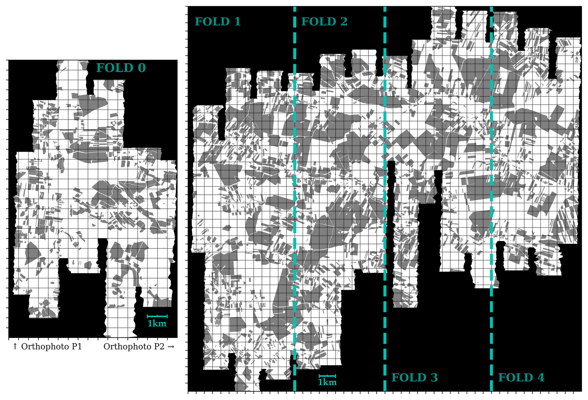
Figure 1 The HyBEAR benchmark patches (grid) overlaid onto the two source orthophotomaps with indication of the divisions into the images and the folds (separated on the maps with the green dashed lines). We depict areas labeled as SOIL using the gray color, NON-SOIL with the white color, and for the regions where we have NO DATA, we use the black color.

3.2 Ground truth preparation

High-quality Ground Truth (GT) is paramount for the validity and utility of any benchmark dataset, particularly in remote sensing applications. Accurate GT labels are essential for training robust machine learning models and for objectively evaluating their performance. The preparation of GT for bare soil detection in HSIs poses unique challenges, including spectral overlap between bare soil and other non-vegetated surfaces (e.g., roads and buildings), as well as the potential for sparse or early-stage vegetation that may be difficult to discern.

In this benchmark, the GT was meticulously prepared through a combination of automated and manual interpretation techniques to ensure high accuracy and reliability. While preparing the manual bare-soil outlines, we considered information from vegetation indices, which are sensitive to chlorophyll and can effectively indicate the absence of mature vegetation. However, relying solely on vegetation indices has limitations. For instance, fresh or very sparse vegetation might not yield a strong enough signal in vegetation indices to be reliably excluded as bare soil. Conversely, non-vegetated areas such as roads, buildings, and artificial surfaces can exhibit low vegetation index values, potentially leading to misclassifications if only this information source is used. Additionally, RGB channels were insufficient for accurate bare soil mapping, primarily because the visual distinction between bare soil and other non-vegetated surfaces can be subtle and is dependent on flight altitude. Also, early or stressed vegetation might not be visually apparent in RGB imagery, leading to errors in GT.

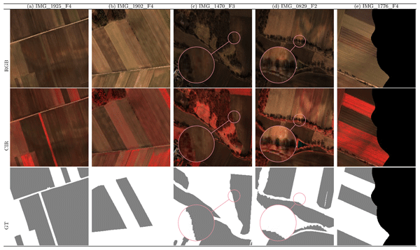
In Fig. 2, several examples of patches are presented. We prepared two different views of the hyperspectral patches: the RGB composition of the bands, and the CIR (Color Infrared using the near-infrared band) image. As one can see, bare soil fields are not easily distinguishable using only RGB images (examples a through e). Relying solely on a CIR image can also be misleading (examples b and e). Objects present in the field of view, such as dirt roads or various shadows, can make identifying the precise borders of bare soil fields difficult, as seen in (c) and (d) of the attached figure (see the zoomed parts of the images and GT masks).

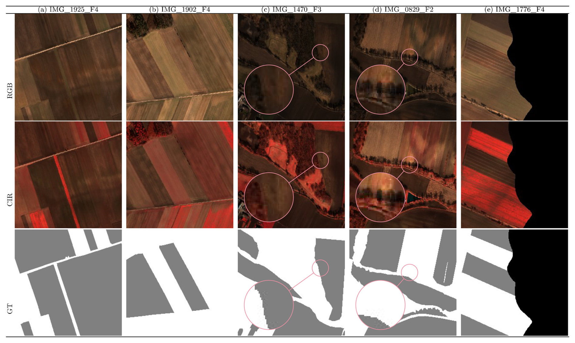
Figure 2 Examples of selected patches from the HyBEAR : (a) RGB images composed of bands 465.3, 532.4, and 628.3 nm of the source hyperspectral patches, (b) CIR images composed of bands 532.4, 628.3, 855.3 nm, and (c) GT  images. We depict areas labeled as SOIL using the gray color, NON-SOIL with the white color, and for the regions where we have NO DATA, we use the black color. The HyBEAR dataset provides original hyperspectral images, RGB, and CIR representations that are composed of 3 bands only and normalized prior to display to enhance their contrast.

To overcome these limitations, a strategy combining the analysis of both vegetation indices and visual information was applied. Initial outlines of potential bare-soil areas were informed by vegetation index analysis, helping identify regions where vegetation was likely absent. Subsequently, these outlines were carefully reviewed and refined by human experts (with 10, 4, and 1 years of hands-on experience), who visually inspected the HSI data and potentially high-resolution RGB imagery (if available). This manual refinement step was crucial for accurately delineating bare soil areas and excluding non-vegetated areas, such as roads, buildings, and shadows, that vegetation indices might have flagged. This iterative process of leveraging automated tools and expert knowledge ensures high accuracy and consistency in the GT labels.

The careful preparation of the GT is a critical aspect that contributes to the remote sensing community. By providing a reliable and accurate reference for bare soil, HyBEAR enables researchers to develop and evaluate algorithms for HSI data analysis, ultimately advancing the field of bare soil detection.

3.2.1 Details of the Manual Labeling Process

To facilitate the manual labeling process², we utilized RGB, CIR, and NDVI band compositions derived from the HSIs. This approach allowed annotators to leverage both natural views and enhanced infrared signals to identify vegetation even in its early growth stages. The annotation team consisted of three experts with 1, 4, and 10 years of experience in remote sensing and agricultural data analysis. The labeling workflow followed an iterative, two-stage process. Initially, the annotators assigned one of two labels: SOIL or MAYBE-SOIL. The SOIL class was strictly reserved for cases where at least approximately 85 % of the parcel surface constituted visible bare soil, exhibiting no distinct indications of mature vegetation. The MAYBE-SOIL label was used as a temporary marker for ambiguous regions, such as fields with sparse emerging plants or high concentrations of crop residues.

To ensure high accuracy and consistency, all MAYBE-SOIL instances were subjected to a consensus-based group discussion involving all three experts. Final decisions for the most challenging cases were moderated by the most senior expert (10 years of experience) to maintain consistency across both geographic locations (P1 and P2). During this refinement, several explicit rules were applied to handle ambiguous cases:

• Crop residues and stubble. Areas were retained in the SOIL class if CIR and NDVI analyses indicated no active photosynthesis, despite the presence of surface organic matter.

• Roads and field margins. Dirt roads and technical infrastructure were manually excluded from the soil polygons by inspecting both hyperspectral data and high-resolution RGB imagery to ensure only the interior of agricultural parcels remained.

• Shadows and moisture. Areas affected by deep shadows (e.g., near tree lines) that obscured the soil's spectral signature were excluded from the SOIL class to ensure the benchmark remains focused on high-quality, interpretable pixels.

This expert-led consensus and the application of the “85 % visibility rule” significantly enhanced the reliability of the ground-truth labels as a reference for cross-location bare soil detection.

3.3 Extraction of image patches

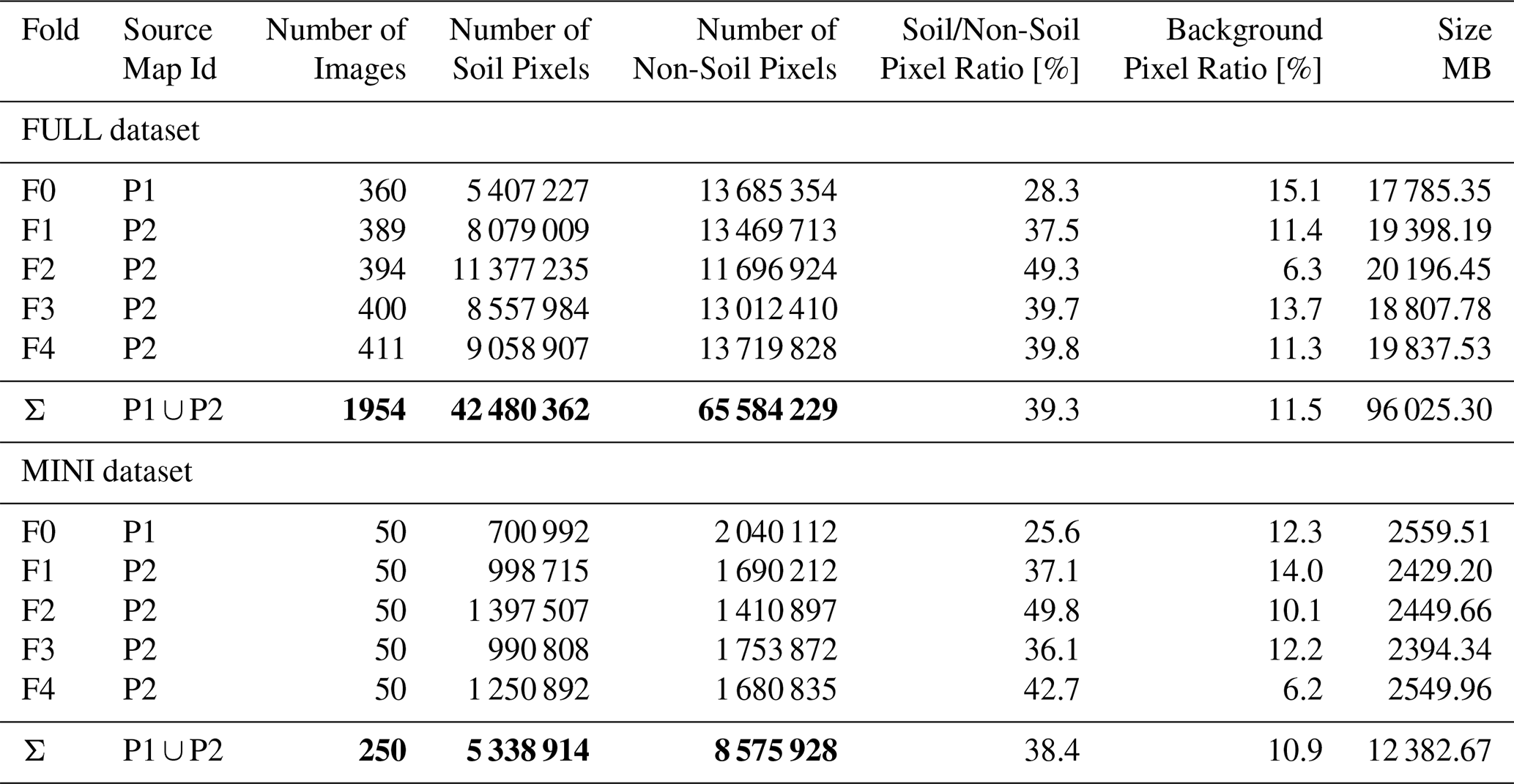
To make the data analysis within HyBEAR more affordable and practical, the large source orthophotomaps were split into smaller image patches. The HyBEAR dataset is composed of 1954 square patches of size 250 × 250 that were extracted from two different source orthophotomaps (P1 and P2). We divided the images according to longitude into five folds (F0, F1, F2, F3, and F4) (Fig. 1). Since the second map is roughly four times larger, we assigned one fold to P1 and four folds to the images extracted from P2 to evenly distribute the images among folds. The presence of NO-DATA pixels in certain patches (visible as black areas in Figs. 1 and 2) is a technical consequence of the irregular geographical boundaries of the flight strips and the subsequent orthorectification process. These regions, which fall outside the actual flight coverage when source orthophotomaps are divided into a regular grid, are encoded with the specific value of −9999 to support their automated filtration. This encoding is a result of the data processing workflow rather than any sensor noise or equipment failure. For each of those patches, in the dataset folder HyBEAR/images/, we store two files: an HSI with 430 spectral bands (IMG_****_F*.TIFF) and the labels' file (GT_****_F*.TIFF), each with its metadata and geospatial information encoded. The name of the file is built using a consecutive file identifier (ID), and a fold number (e.g., IMG_0555_F1.TIFF). In addition to the full version of the HyBEAR dataset, we offer a lighter version of our collection, referred to as the MINI subset of HyBEAR. To create the MINI subset, we selected exactly 50 images from each fold using stratified random sampling (with a fixed random seed of 171) based on the proportion of soil pixels. This procedure ensures that the MINI collection maintains a balanced and reproducible representation of the geographical diversity found in the FULL dataset. The dataset statistics are summarized in Table 1.

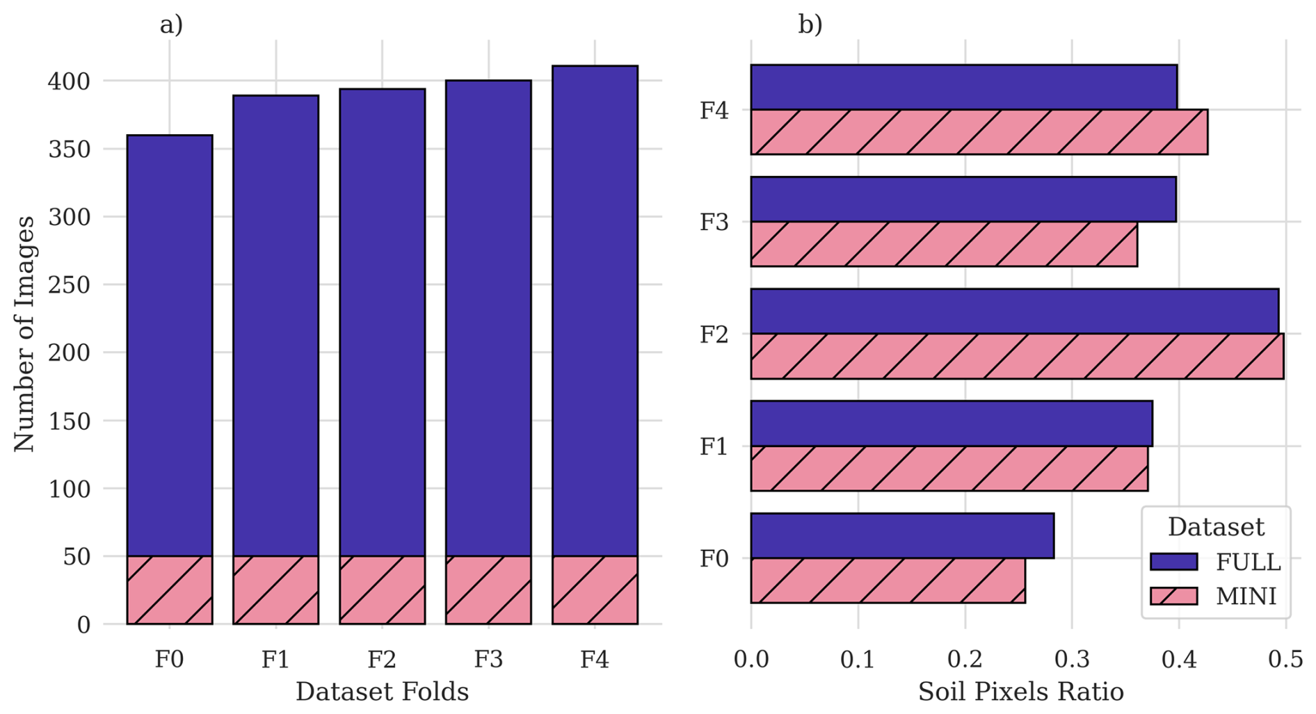
Figure 3 The HyBEAR dataset details summary. On the left: (a) we depict the number of images for every fold and MINI subsets. On the right: (b) we visualize the proportion of the soil and non-soil classes across all folds and subsets (for the FULL and MINI versions of the dataset).

Table 1 The HyBEAR dataset structure and descriptive statistics. Please append the table caption wtih the text: “Bolded values indicate summary statistics for FULL and MINI datasets”.

It is worth noting that the primary reason we chose to use the TIFF file format for all images is that it allows us to include geolocation information for each patch. Also, it preserves the full image encoding precision and supports decent data compression. For HyBEAR, we selected a lossless deflate compression method that reduced the average patch size from approx. 215 MB per image to around 40–48 MB.

The resulting image collection was tested using two different environments: QGIS (versions 3.28 and 3.40) and a Python-based application (employing Rasterio, NumPy, and Scikit-Learn libraries – the configuration file of the Python environment, as well as the code we use for testing, is delivered with this dataset to support reproducibility).

3.4 Cross-validation protocol

The HyBEAR dataset consists of two independent aerial hyperspectral scenes, P1 and P2, which were carefully selected to enable a comprehensive and rigorous evaluation of algorithms dedicated to bare soil detection. One of the key aspects of HyBEAR is the evaluation protocol, based on the multi-fold cross-validation scenarios. To verify the generalization capability of the bare soil detection methods, as well as their robustness to the variability of the acquired data, we defined the experimental scenarios within a five-fold cross-validation framework:

• Stage 1. Training an algorithm on the folds F1 to F4 (T_F1:F4) → testing on the fold F0 (Ψ_F0).

• Stage 2. Training an algorithm on the folds 𝙵≠𝟷 (${\mathit{T}}_{\mathrm{F}\mathrm{0},\mathrm{F}\mathrm{2}:\mathrm{F}\mathrm{4}}$) → testing on the fold F1 (Ψ_F1).

• Stage 3. Training an algorithm on the folds 𝙵≠𝟸 (${\mathit{T}}_{\mathrm{F}\mathrm{0}:\mathrm{F}\mathrm{1},\mathrm{F}\mathrm{3}:\mathrm{F}\mathrm{4}}$) → testing on the fold F2 (Ψ_F2).

• Stage 4. Training an algorithm on the folds 𝙵≠𝟹 (${\mathit{T}}_{\mathrm{F}\mathrm{0}:\mathrm{F}\mathrm{2},\mathrm{F}\mathrm{4}}$) → testing on the fold F3 (Ψ_F3).

• Stage 5. Training an algorithm on the folds 𝙵≠𝟺 (T_F0:F3) → testing on the fold F4 (Ψ_F4).

This evaluation protocol has been designed with several key objectives in mind, relevant to the evaluation of algorithms in the context of real-world applications of bare soil detection from aerial data:

• Evaluation of generalization to spatially independent areas. The hyperspectral scenes P1 (F0) and P2 (F1 : F4) represent data acquired from different geographical locations. Testing on one area after training on the other allows a direct assessment of the algorithm's ability to generalize knowledge to new, previously unseen areas. This is crucial, as in practice, models are rarely applied to exactly the same areas where they were trained.

• Verification of robustness to the variability of acquisition conditions. Aerial data can exhibit significant spectral and spatial variability depending on atmospheric conditions, illumination, season, or sensor configuration. Our evaluation protocol, by testing on spatially disjoint areas (P1 and P2, see Fig. 1), enables the assessment of the algorithms' robustness to such factors. An algorithm that performs well in both scenarios demonstrates greater reliability.

• Preventing overfitting to the specifics of a single dataset. Training and testing on the same dataset can lead to inflated performance evaluations if the model learns specific characteristics of that dataset that are not universal. Our cross-validation protocol minimizes this risk by forcing the model to learn more general and representative features of bare soil.

• Enabling comparability of results. Defining clear data splitting scenarios as part of the benchmark ensures that different bare soil detection methods can be evaluated in a consistent and comparable manner. This allows researchers to objectively quantify and assess the progress in this field.

To facilitate a fair comparison of different bare soil detection methods, the following commonly adopted classification and segmentation metrics will be used to quantitatively evaluate the models within the presented evaluation protocol – these metrics are presented in the next section.

3.5 Evaluation metrics

To evaluate the performance of the emerging ML models, a series of commonly adopted classification metrics is used (Powers, 2011). This choice is motivated by the need for a comprehensive analysis of the models' ability to correctly identify bare soil pixels.

• Accuracy (ACC) measures the overall percentage of correctly classified samples, and it is calculated as:

  $$\begin{array}{}\text{(1)}& \mathrm{ACC}={\displaystyle \frac{\mathrm{TP}+\mathrm{TN}}{\mathrm{TP}+\mathrm{TN}+\mathrm{FP}+\mathrm{FN}}},\end{array}$$

  where TP, TN, FP, and FN represent true positives (correctly classified bare soil image pixels), true negatives (correctly classified non-bare soil image pixels), false positives (the non-bare soil image pixels incorrectly classified as those containing bare soil), and false negatives (bare soil image pixels incorrectly classified as the non-bare soil image pixels). Accuracy represents a fundamental measure of classification effectiveness.

• Sensitivity (SEN) determines the model's ability to identify all actual positive cases (bare soil image pixels):

  $$\begin{array}{}\text{(2)}& \mathrm{SEN}={\displaystyle \frac{\mathrm{TP}}{\mathrm{TP}+\mathrm{FN}}}.\end{array}$$

  High sensitivity is crucial for minimizing bare soil omissions (false negatives).

• Specificity (SPE) measures the model's ability to correctly identify all actual negative cases (image pixels not containing bare soil):

  $$\begin{array}{}\text{(3)}& \mathrm{SPE}={\displaystyle \frac{\mathrm{TN}}{\mathrm{TN}+\mathrm{FP}}}.\end{array}$$

  High specificity ensures that the model rarely generates false-positive detections.

• F-score (F1) represents the harmonic mean of precision ($\frac{\mathrm{TP}}{\mathrm{TP}+\mathrm{FP}}$) and sensitivity, providing a balanced measure of performance, particularly important for potentially imbalanced datasets:

  $$\begin{array}{}\text{(4)}& \mathrm{F}\mathrm{1}=\mathrm{2}\cdot {\displaystyle \frac{\text{Precision}\cdot \text{Sensitivity}}{\text{Precision}+\text{Sensitivity}}}={\displaystyle \frac{\mathrm{2}\cdot \mathrm{TP}}{\mathrm{2}\cdot \mathrm{TP}+\mathrm{FP}+\mathrm{FN}}}.\end{array}$$

• Intersection over Union (IoU) measures the degree of overlap between the predicted and actual positive outcomes. It is particularly useful for evaluating the quality of segmentation or object detection. It is calculated as the ratio of the intersection of the sets of predicted positives and actual positives to their union:

  $$\begin{array}{}\text{(5)}& \mathrm{IoU}={\displaystyle \frac{\mathrm{TP}}{\mathrm{TP}+\mathrm{FP}+\mathrm{FN}}}.\end{array}$$

• Matthews Correlation Coefficient (MCC) is a measure of the correlation between observed and predicted binary classifications, more robust to imbalanced data than ACC or F1 (Chicco et al., 2021). It is calculated as:

  $$\begin{array}{}\text{(6)}& \mathrm{MCC}={\displaystyle \frac{\mathrm{TP}\cdot \mathrm{TN}-\mathrm{FP}\cdot \mathrm{FN}}{\sqrt{(\mathrm{TP}+\mathrm{FP})(\mathrm{TP}+\mathrm{FN})(\mathrm{TN}+\mathrm{FP})(\mathrm{TN}+\mathrm{FN})}}}.\end{array}$$

• The Receiver Operating Characteristic (ROC) curve illustrates the relationship between SEN and (1−SPE) for various classification thresholds (Powers, 2011). The Area Under this Curve (AUC) quantifies the overall ability of the model to discriminate between classes, where higher AUC values indicate better performance.

Collectively, these metrics are crucial to provide a comprehensive, objective, and standardized way to assess and compare the performance of various methods in the bare soil detection task.

3.6 Dataset organization

The data is organized in the following directory structure:

• HyBEAR/ – the main directory serving as the root for the entire dataset. It contains all the necessary files and subdirectories to organize the hyperspectral patches and their corresponding GTs for both P1 and P2.

• HyBEAR/images/ – this directory is the core of the dataset, containing the extracted hyperspectral patches and their associated GTs. This organization allows for direct access to the data for training and testing purposes:

  • HyBEAR/images/F0_FULL/, …, HyBEAR/images/F4_FULL/,
    HyBEAR/images/F0_MINI/, …, HyBEAR/images/F4_MINI/ – these directories contain the TIFF image patches and the GT patches for folds F0 : F4, and for MINI or FULL subset.

• HyBEAR/wavelengths.csv – a metadata file providing the spectral characteristics of the 430 bands in the hyperspectral images. It contains two columns: Wavelength, representing the center wavelength for each specific spectral band, and Full Width at Half Maximum (FWHM), which specifies the spectral width of the band measured at half of its maximum intensity. This file allows for the correct physical interpretation of the spectral data without the need to inspect the source code.

• HyBEAR/code/ – this directory stores several Python Jupyter Notebook files for the initial dataset presentation, displaying the hyperspectral patches and their associated GTs, and reproducing the reported benchmark results. It includes the baseline_model_training.ipynb, which provides the complete training workflow – including preprocessing, normalization, random seeds, and hyperparameters – ensuring full transparency and reproducibility of the benchmark. It also contains the configuration file for the required Python libraries.

• HyBEAR/models/ – this directory contains the models trained using HyBEAR under the suggested 5-fold cross-validation regime. We deliver models for each validation phase and for two different machine learning algorithms (Logistic Regression and Support Vector Machines). Therefore, this folder contains 10 files. These models can be verified using the HyBEAR/code/model_evaluation.ipynb that was developed to support the classification of each hyperspectral image and pixel.

The hyperspectral image patches (files from IMG_0000_F0.tiff to IMG_1953_F4.tiff) contain information about the light reflectance values in different spectral ranges for each pixel. The GT patches (files from GT_0000_F0.tiff to GT_1953_F4.tiff) store binary information and indicate which pixels in the hyperspectral patch belong to:

• the SOIL class – encoded as (1),

• and which do not depict SOIL (hence, are NON-SOIL) – encoded as (0),

• additionally, for the pixels extracted from the edges of the main hyperspectral scene that do not contain data in the image, we use the code (-9999) and encode them in the GT images as background, thereby supporting their automated filtration.

The patches have fixed dimensions of 250 × 250 pixels and were generated using a grid-based method from the original hyperspectral scenes P1 and P2. The dataset (consisting of these patches) is available at https://doi.org/10.5281/zenodo.17607897 (Wijata et al., 2025). The entire dataset comprises 1954 data tuples and has a total size of 96 GB (for the compressed files, with the average size of a single tuple being 48 MB).

4 Experiments and baseline results

4.1 Methods

In addition to the dataset, several machine learning models were evaluated under the introduced cross-validation regime. We trained models on the hyperspectral pixels extracted separately from each image, and we employed the standard machine learning model architectures: Logistic Regression (later denoted as LR), Linear models with L₂ Regularization (L₂), Adaptive Boosting (AB), Support Vector Machines with a linear kernel (SVM), Decision Trees (DT), and Random Forest (RF). All models operate on feature vectors of size 430, which are the values of all spectral bands captured within a particular pixel. The selected models enable the efficient processing of the extensive HyBEAR dataset, for which the number of pixels for an image could reach 62 500. Since the number of images in each fold varies, and as we exclude the background pixels that do not contain any data, the overall number of training samples varies accordingly. The ratio of “useful” pixels (excluding background) for each fold is reported in Table 1.

4.2 Baseline results

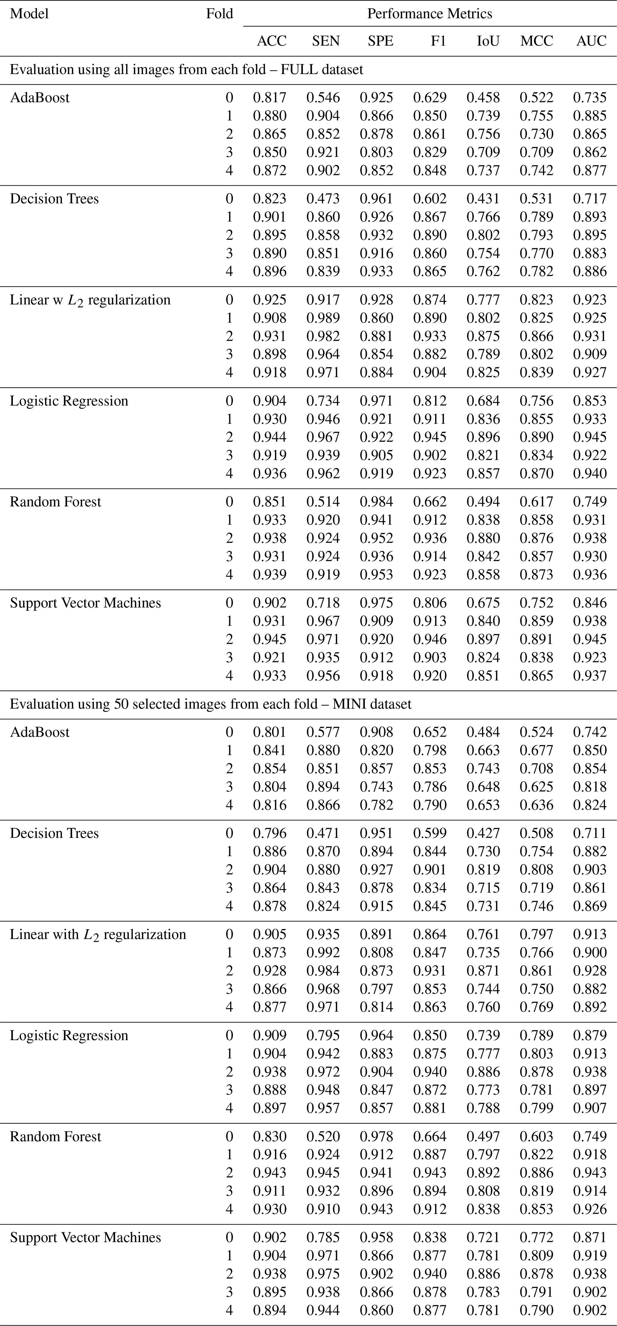
In the experiments, we exploit both versions of the HyBEAR benchmark, with all the images (FULL) and using only a subset of 50 images from each fold (MINI). Table 2 provides the aggregated metrics, together with their standard deviation. The detailed results of every fold are gathered in the appendix (Table A1). Additionally, the results are depicted in Fig. 4. Here, in addition to the metrics computed for every fold (points on the dashed lines), we plotted the average metric levels (dotted lines). Following this visualization should allow for spotting the models that are more consistent across the folds, and therefore, would return a more robust and universal classifier.

Table 2 The HyBEAR benchmark baseline results (the average and standard deviation, μ±σ) averaged after the 5-fold cross-validation procedure. The best results for each metric are boldfaced.

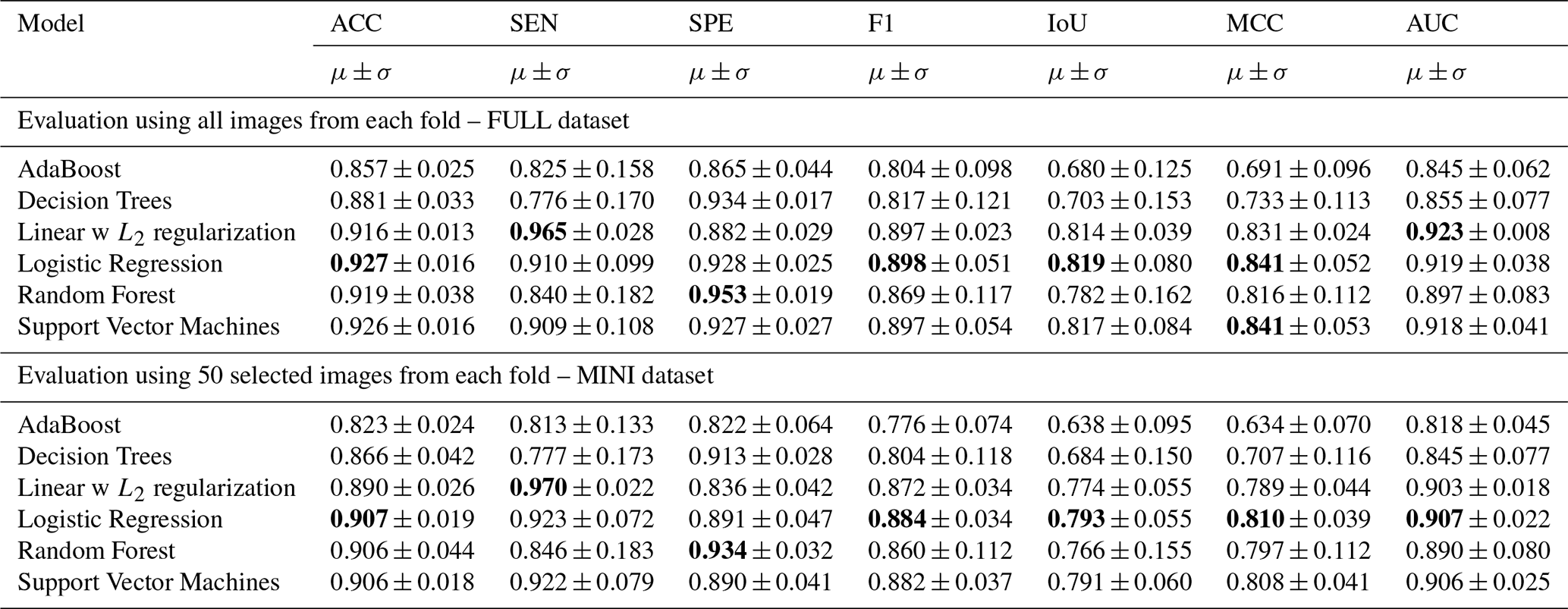
The highest performance scores were obtained for the LR-based models for the majority of metrics, with the SVM-based models reaching nearly the same performance, both for the FULL and MINI versions of HyBEAR. In Fig. 5, we present three example patches with the GT labels and the corresponding predictions elaborated using the investigated machine learning models. Here, the red areas show the false-positive bare-soil detections, whereas the yellow areas correspond to the false-negative detections. The average accuracy for some models reached a decent level of 0.926–0.927 (for SVM and LR, respectively), and the F-score was almost 0.9 (0.898 for the best-performing LR model). When previewing the predictions for these models over the example test patches (Fig. 5), we can observe that there is still significant room for improvement for most of the models. For some less challenging patches (i.e., IMG_0717_F1), the results are satisfactory, but for some others (i.e., IMG_0022_F0), most of the models perform poorly. The performance drop observed in Fold 0 is particularly noteworthy, as it serves as the primary benchmark for cross-location generalization within HyBEAR (Table A1 and Fig. 4). While Folds 1–4 are derived from scene P2, Fold 0 is the only fold extracted from scene P1, located more than 60 km away. Despite the data being acquired on the same day, the dynamic position of the sun and clouds resulted in varying lighting conditions and reflectance levels between these geographic areas. This domain shift is the primary reason why non-linear models like Random Forest, AdaBoost, and Decision Trees – which likely overfitted the specific spectral characteristics of the larger P2 scene – showed significant degradation in sensitivity and F1-scores when applied to Fold 0. In contrast, simpler linear models (LR, SVM) proved to be more robust and universal in this cross-location scenario.

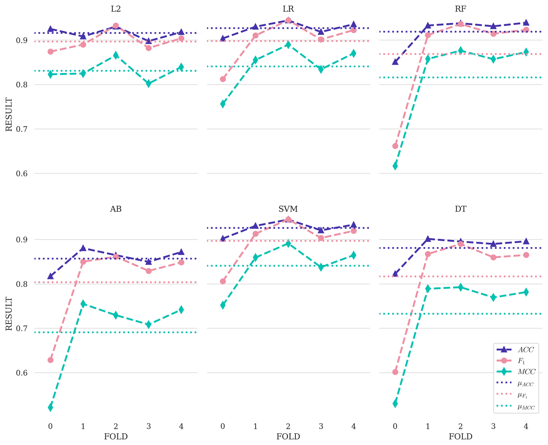
Figure 4 The benchmarking results for the investigated machine learning models. We present the results for each fold separately, along with the average result for each metric (dotted line).

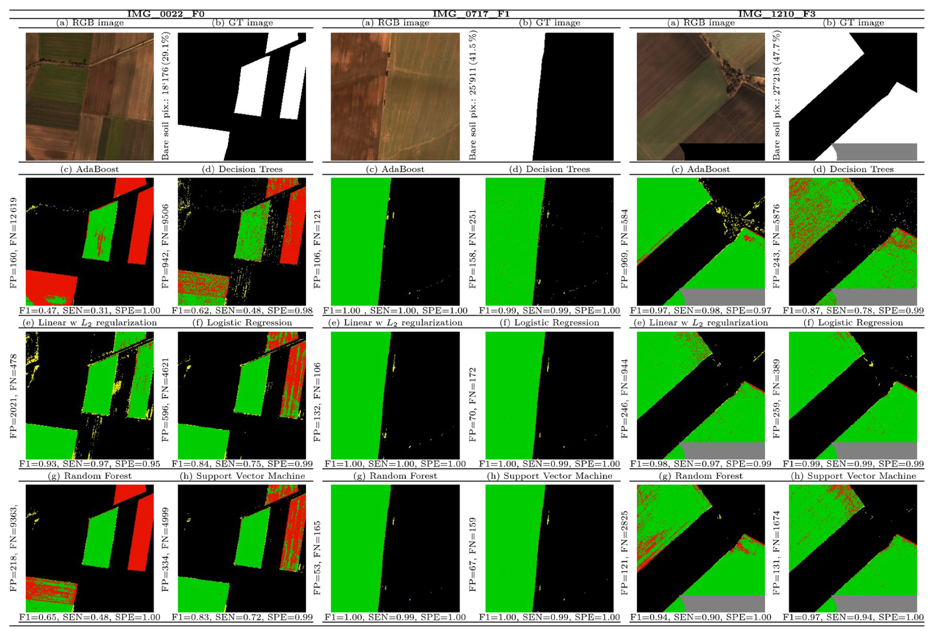
Figure 5 Example bare soil detection results with the quantitative metrics: (a) RGB images with (b) GT marked in white, (c–h) various prediction methods (TP – green, FP – yellow, FN – red, TN – black, missing data/background – gray).

Furthermore, Fold 0 presents an inherently greater difficulty due to class imbalance, as it contains the lowest soil pixel ratio in the dataset (28.3 % for FULL and 25.6 % for MINI). Qualitative inspection of failure cases, such as IMG_0022 _F0 (Fig. 5) reveals that errors are often caused by physical factors like tree shadows and dirt roads that might mimic bare soil, or crop residues that introduce spectral mixing. These results suggest that capturing more complex spatial relationships through, e.g., automated representation learning in deep learning models, may be necessary to further boost the capabilities of the detectors.

5 Code and data availability

We published HyBEAR  – Wijata et al. (2025) on Zenodo: https://doi.org/10.5281/zenodo.17607897. In addition to the hyperspectral images and ground-truth labels, this package includes the full testing procedure for all baseline machine learning models reported in this study. To ensure reproducibility, we provide the original Python scripts and Jupyter Notebooks covering the core stages of the data evaluation chain: preprocessing, normalization, and the 5-fold cross-validation logic. Furthermore, the repository contains the final trained models and the evaluation code, allowing researchers to independently verify the presented benchmark results.

6 Conclusions

Bare soil detection is an important task in precision agriculture, as it allows for determining the areas in Earth observation imagery that shall be further analyzed while estimating specific soil parameters and features. In this paper, we introduced HyBEAR – a comprehensive hyperspectral benchmark dataset, accompanied by the baseline results for automated bare soil detection from HSIs. The provided large-scale data collection delivers high-resolution hyperspectral imagery (with the 2 m GSD), together with the carefully prepared ground-truth delineations of bare soil areas. These annotations were meticulously verified in collaboration with domain experts who routinely analyze soil samples. Finally, the provided airborne imagery is free of disturbances, with no cloud cover or dust in the camera's field of view. To our knowledge, the HyBEAR dataset is the first in the literature that offers bare soil pixels captured for specific agricultural parcels (i.e., it is not a set of spatially unaware multi/hyperspectral pixels). Therefore, it may be utilized in practical examples where delineating the field boundaries is key. HyBEAR defines the five-fold cross-validation procedure and is accompanied by the baseline results. We strive to ensure full reproducibility of any research that will emerge based on the provided benchmark, and thus have made our implementations and code examples publicly available.

The experimental results reported in this work will serve as the point of departure for future work, potentially in a multitude of use cases related to hyperspectral data analysis. The quantitative and qualitative results showed that there are areas where classic machine learning models (operating on spectral curves for each hyperspectral pixel) fail to appropriately identify bare soil. Thus, extracting more discriminative features and leveraging automated representation learning offered by deep learning (Guerri et al., 2024) would likely lead to higher-quality bare soil detection. It is important to emphasize that the HyBEAR dataset may be exploited for other tasks, such as feature extraction (Zhang et al., 2024), feature selection (Tan et al., 2025), unsupervised clustering/domain adaptation (Cai et al., 2024), and many more.

6.1 Limitations

Despite the significant scale and high resolution of the HyBEAR benchmark, several limitations should be acknowledged. First, the dataset represents a regional and temporal snapshot, as it was acquired in Southern Poland on a single day in early spring. Consequently, it may not capture the full spectral variability of all global soil types or the influence of diverse seasonal and climatic conditions. Second, while the benchmark provides unique parcel-level annotations, our current baseline experiments are primarily pixel-wise. These results serve as a fundamental performance reference but do not yet fully exploit the contextual, field-level nature of the annotations for advanced parcel-based decision-making. Finally, although the evaluation protocol employs spatially disjoint scenes (P1 and P2), the benchmark primarily addresses regional cross-location generalization rather than global agroecological robustness. Future expansions of HyBEAR are intended to incorporate data from more diverse geographic zones and timeframes to address these constraints.

6.2 Practical Applications and Future Work

The HyBEAR benchmark is designed to support a wide range of practical applications in Earth observation:

• Precision Agriculture. The provided bare soil masks enable targeted parcel-based fertilization planning and accurate soil property mapping, ensuring that analytical models for moisture or organic matter are applied only to relevant pixels.

• Environmental Monitoring. The dataset facilitates large-scale tracking of agricultural practices, such as tillage and fallow periods, and supports the identification of areas at risk of soil erosion.

• On-board Data Compression. HyBEAR serves as a testing ground for “smart data compression” algorithms on satellite edge devices. By pruning non-soil areas directly on orbit, transmission volumes can be drastically reduced, making hyperspectral data analysis more memory-efficient.

Future work will focus on leveraging automated representation learning through deep learning architectures to capture more complex intrinsic soil features and spatial relationships. Furthermore, we intend to expand HyBEAR with data from diverse geographic zones to enhance its global representative value.

Appendix A: Detailed experimental results

Table A1 The detailed results for all evaluated algorithms, computed under a 5-fold cross-validation regime in two variants: using all available images (FULL) and the MINI subset.