the Creative Commons Attribution 4.0 License.
the Creative Commons Attribution 4.0 License.
 | 05 Oct 2026
A benchmark dataset of water levels and waves for SWOT validation in the St. Lawrence Estuary and Saguenay Fjord, Quebec, Canada

Xavier Chartrand
David Purnell
Marc Simard
Alexandra Christensen
Francis Fortin-Legault
Jonathan Morin
Yann Côté-Nadeau
Élaine Desrosiers
Anthony Ouellet
Cédric Chavanne
François Anctil
Gabriela Siles
Scott Bedart
Silvia Innocenti
Mohammed Dabboor
Daniel L. Peters
Mélanie Trudel
This manuscript presents a comprehensive and evolving in situ dataset of water levels and wave parameters collected from March 2023 onward in the St. Lawrence Estuary and Saguenay Fjord (Quebec, Canada), supporting validation activities for the Surface Water and Ocean Topography (SWOT) satellite mission. The dataset integrates water level measurements from 18 barometrically compensated pressure transducers, where possible corrected for water density using collocated salinity and temperature data, supplemented with 13 GNSS-Interferometric Reflectometry (GNSS-IR) sensors. All water level data are referenced to a common vertical datum via real-time kinematic (RTK) GNSS corrections. Three directional wave buoys provided supplementary observations of surface wave conditions, including bulk parameters and directional spectra. Quality-controlled and rigorous processing protocols were implemented across all sensor types, with particular attention to referencing accuracy and correction for environmental influences. The observational network has the densest spatial coverage of water level and wave measurements ever achieved in this region, offering unprecedented opportunities to support the validation of SWOT’s nadir and wide-swath altimetry products, as well as for hydrodynamic model calibration and spatio-temporal studies of tidal and wave processes in complex estuarine environments. With ongoing data collection, this evolving benchmark dataset is publicly accessible at https://doi.org/10.5281/zenodo.18225504 (Matte et al., 2026) and will be updated approximately annually, as new observations are retrieved, processed, and quality controlled, to support continued SWOT validation throughout the mission and a broad range of estuarine research applications.
- Article
(10964 KB) - Full-text XML
- BibTeX
- EndNote


The works published in this journal are distributed under the Creative Commons Attribution 4.0 License. This licence does not affect the Crown copyright work, which is re-usable under the Open Government Licence (OGL). The Creative Commons Attribution 4.0 License and the OGL are interoperable and do not conflict with, reduce or limit each other. © Crown copyright 2026
Estuaries are critically important ecosystems. They provide essential habitat for a wide variety of marine species, including many of commercial and recreational value, and help protect coastal communities by buffering storm impacts and filtering pollutants. Given their ecological and economic significance, as well as their vulnerability to human pressures and climate change, sustained monitoring is essential to ensure their long-term health and productivity (Ward et al., 2020). Particularly critical are the upper estuarine transitional zones, which face the highest risk of a significant reduction in extent, a process termed “estuarine squeeze” by Little et al. (2022). This occurs when rising sea levels and reduced river flows push saltwater inland while man-made barriers prevent the natural landward migration of these habitats, leading to their progressive loss and the degradation of key ecosystem services.
A combination of data from monitoring networks and numerical model simulations is typically required in these regions to support dynamical analyses and to inform the implementation of integrated water resources management (Meran et al., 2021). The number of active in situ gauges for discharge monitoring has declined globally (Elmi et al., 2024; Mishra and Coulibaly, 2009), whereas tide gauge records have benefited from expanding databases obtained by consolidating diverse data sources (Haigh et al., 2023). Critically, the global distribution of such stations remains spatially uneven, and despite the extensive number of gauges, existing monitoring networks may struggle or in some instance can fail to capture the intricate flow dynamics within complex systems like deltas and wetlands. Likewise, the calibration of hydrodynamic models requires spatio-temporally comprehensive observations, which are frequently lacking, especially in remote regions of the globe. The Surface Water and Ocean Topography (SWOT) satellite mission holds promise as an enhancement of and potentially an alternative to existing gauge networks for monitoring surface water conditions within the land-ocean aquatic continuum (LOAC) and for facilitating model calibration. SWOT is the first satellite of its kind designed to collect two-dimensional water level data at unprecedented resolution, thanks to its innovative dual antenna Ka-band radar interferometer (KaRIn) (Fu et al., 2024). After a successful launch in December 2022 and a subsequent three-month commissioning period, SWOT began a three-month Calibration/Validation (Cal/Val) phase in late March 2023 ending on 11 July 2023. During this Cal/Val phase, SWOT collected near-daily observations of the water surface, at low resolution over oceans and at high resolution over terrestrial water bodies. Only a few estuaries worldwide were covered by this fast-sampling orbit, benefiting from both low- and high-resolution data at the LOAC. Among them are the St. Lawrence Estuary and Saguenay Fjord in Quebec, Canada, which represent the most heterogeneous and dynamically complex regions of the St. Lawrence system (SLS).
Specifically, these two regions include (1) the St. Lawrence estuarine transition zone (Simons et al., 2010), encompassing the saltwater intrusion limit and experiencing large tidal ranges reaching 7 m; and (2) the head of the Laurentian Channel near the mouth of the Saguenay Fjord, an area of steep seafloor slope known as a hotspot for internal tide generation, and populated with eddies and fronts (Mertz et al., 1988; El-Sabh et al., 1982; Forrester, 1974). Given the unique characteristics of these two sites, the SWOT satellite's daily overpasses offered a groundbreaking opportunity to gather detailed spatio-temporal data on local estuarine dynamics in this region, as well as to colligate already established networks with additional in situ observations focused on validating the new SWOT wide-swath altimetry products in a macro-tidal fluvial-estuarine setting (d'Ovidio et al., 2019).
Beyond spatial and temporal coverage, the validation of SWOT water surface elevation products depends critically on the accuracy of the reference observations. Validation at the decimetric scale in absolute water level requires ground-based measurements with higher accuracy and well-characterized uncertainties. This constraint underscores the need for careful sensor deployment, calibration, and processing, and for independent validation of the reference observations through a dedicated field campaign prior to their use in assessing SWOT performance.
To meet these accuracy and validation requirements, starting in March 2023, an extensive field campaign was conducted in the St. Lawrence Estuary and Saguenay Fjord to strategically expand the existing network of monitoring stations with additional observations and supporting data to enable SWOT validation. Water levels, waves, and auxiliary variables characterizing sea surface conditions of the SLS were measured using an array of sophisticated instruments that included pressure gauges, low-cost Global Navigation Satellite System Interferometric Reflectometry (GNSS-IR) sensors, wave buoys, high frequency (HF) radars, fixed (horizontal) and boat-mounted acoustic Doppler current profilers (ADCPs), AirSWOT (an Airborne Ka-band interferometric synthetic aperture radar analog to SWOT), and ancillary satellite data (e.g., RADARSAT Constellation Mission).
While the initial focus was on the SWOT Cal/Val period and its associated orbit footprint, most stations continued to operate after the satellite moved to its final 21 d repeat Science orbit. Similarly, the AirSWOT flights were conducted in late August 2023, coinciding with SWOT overpasses at the beginning of the Science phase (Simard et al., 2023). As a result, a vast and constantly expanding dataset of water surface conditions is now available from a dense network of monitoring stations and measurement platforms, offering detailed validation data that covers both ice and open-water seasons, for a wide range of hydrological and meteorological conditions, and topographical settings.
This article introduces this new and growing dataset of in situ observations, with a focus on water level and wave data from pressure gauges, GNSS-IR sensors, and wave buoys. The broader observing effort also included HF radars, ADCPs, AirSWOT, and ancillary satellite observations. These complementary datasets are not included in the present data release because each requires dedicated processing and validation workflows to produce scientifically robust products suitable for SWOT validation. They will be described and documented separately.
The manuscript is organized as follows. Section 2 presents the study sites along with the instrumental network situated within or adjacent to the SWOT Cal/Val orbit track. Details of the experimental design, acquisition methods, processing steps and quality control for each type of instruments are presented in Sect. 3. A complete description of datasets, data content and format is found in Sect. 4. Validation results including examples of representative data are presented and discussed in regard of uncertainties and limitations, in Sect. 5. Supplementary code and data processing workflows are presented in Sect. 6. Finally, Sect. 7 provides a summary and perspectives on future uses of this novel benchmark dataset for SWOT validation and beyond. The database is available at https://doi.org/10.5281/zenodo.18225504 (Matte et al., 2026).
2.1 St. Lawrence Estuary
The Great Lakes/St. Lawrence basin holds 25 % of the world’s freshwater, covering an area of 1.6 million km2. The average St. Lawrence River discharge at Quebec City site amounts to 12 200 m3 s−1 and reaches 16 800 m3 s−1 passed the Saguenay Fjord. Daily mean discharges can more than double during the spring freshet season, while peak tidal discharges can reach up to five times the daily average (Bourgault and Matte, 2020). Due to its converging shape, propagating tides in the St. Lawrence are amplified up to the estuarine transition zone, upstream of which they are progressively damped by bottom friction and river flow (Godin, 1999; Matte et al., 2017a, b). The large estuarine widths of several tens of kilometers lead to spatially heterogeneous tides with larger amplitudes typically observed on the North shore. In addition to tides, nearby and distant storm surges associated with strong winds and low air pressure contribute to elevated total water levels in the St. Lawrence Estuary and Gulf, leading to extreme flooding conditions when different surge components coincide with high tide (Bourgault et al., 2016a; Mulligan et al., 2023). Similarly, the joint occurrence of high river flow and high coastal water levels increases the risk of flooding, which is likely to be exacerbated by sea-level rise for the coasts of the Estuary and Gulf (Bizhanimanzar et al., 2024).
The gravity and vorticity wave field of the St. Lawrence Estuary exhibits marked spatial heterogeneity that is closely tied to water depth, seafloor slopes, cross-sectional widths and tidal amplification, whose factors vary considerably across the basin. The Upper Estuary, extending from the Orleans Island to Tadoussac, features uneven bathymetry, with deep troughs, shallow banks, islands and ridges. Conversely, the Lower Estuary from Tadoussac to Pointes-des-Monts is much deeper and encompasses the Laurentian Trough, which drops to a depth of more than 300 m, contrasting with a gentle bottom slope on its south shore shelf. As a result, a broad spectrum of waves is observed along the river, from supra-inertial motions, such as internal waves and tides in the Upper Estuary (Bourgault and Kelley, 2003), to strong sub-inertial motions in the Lower Estuary, including topographic waves and unstable shear waves (Mertz and Gratton, 1990). Historical data on surface gravity waves during the ice-free period indicate that they are mainly influenced by orographic factors. Wave provenance is strongly aligned with prevailing winds blowing along the St. Lawrence Lower Estuary, with significant wave heights ranging from a few tenths of a meter to a few meters, while peak heights can surpass several meters (Ruest et al., 2013). Analyzing wave conditions and climate in the St. Lawrence throughout the annual cycle remains challenging, as the presence of sea ice poses significant risks to wave buoys and requires the inclusion of robust wave-ice parameterizations in numerical models. Developing such parameterizations is still an active area of research, yet essential for accurate wave climate hindcasts.
2.2 Saguenay Fjord
The Saguenay Fjord is the second-largest tributary of the SLS, with a watershed area of 88 000 km2 and an average discharge of 1750 m3 s−1. It is one of the southernmost fjords in the Northern Hemisphere, yet seasonally ice-covered, and possesses the unique attribute of being intracontinental. Surrounded by tall cliffs peaking at 350 m in height, this water body plunges to comparable depths (<270 m) before rising sharply towards a series of sills that culminate at a depth of 20 m in Tadoussac, located at the mouth of the Fjord. Contrary to the St Lawrence Estuary, the Saguenay Fjord width narrows towards its mouth, from 3.5 km near Port Alfred to 1.1 km in Tadoussac (Belzile et al., 2016). Despite its divergent widths, tides increase in intensity as they move inland, reaching heights of approximately 3 and 6 m at the Fjord's mouth to between 4 and 7 m at Port Alfred, during neap and spring tides, respectively. Moreover, tides behave like a standing, rather than a propagating wave, resulting in quasi-synchronous high and low tides throughout the Fjord, and correspondingly low instantaneous water surface slopes during most of the tidal cycle. It is also a region where the generation of internal solitary waves has been documented (Bourgault et al., 2016b).
This section describes the instrumentation used to measure water levels and waves, their deployment sites, data acquisition methods, processing procedures, and the various quality control levels applied.
3.1 Water level data and instrumentation
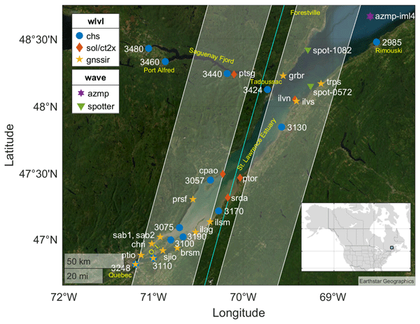
The existing network of permanent stations maintained by the Canadian Hydrographic Service (CHS) is composed of only 9 tide gauges in the study area: 6 in the St. Lawrence Estuary between Quebec (3248) and Rimouski (2985), and 3 in the Saguenay Fjord between Baie-Sainte-Catherine (3424) and Chicoutimi (3480). To better capture the system dynamics and its spatio-temporal variability during the SWOT Cal/Val phase, we installed an additional 22 water level stations on both shores of the St. Lawrence as well as on islands, resulting in an augmented network of 31 water level stations. Figure 1 displays the locations of the water level stations within the study area under the SWOT Cal/Val orbit, that were strategically distributed across each swath and under the nadir.
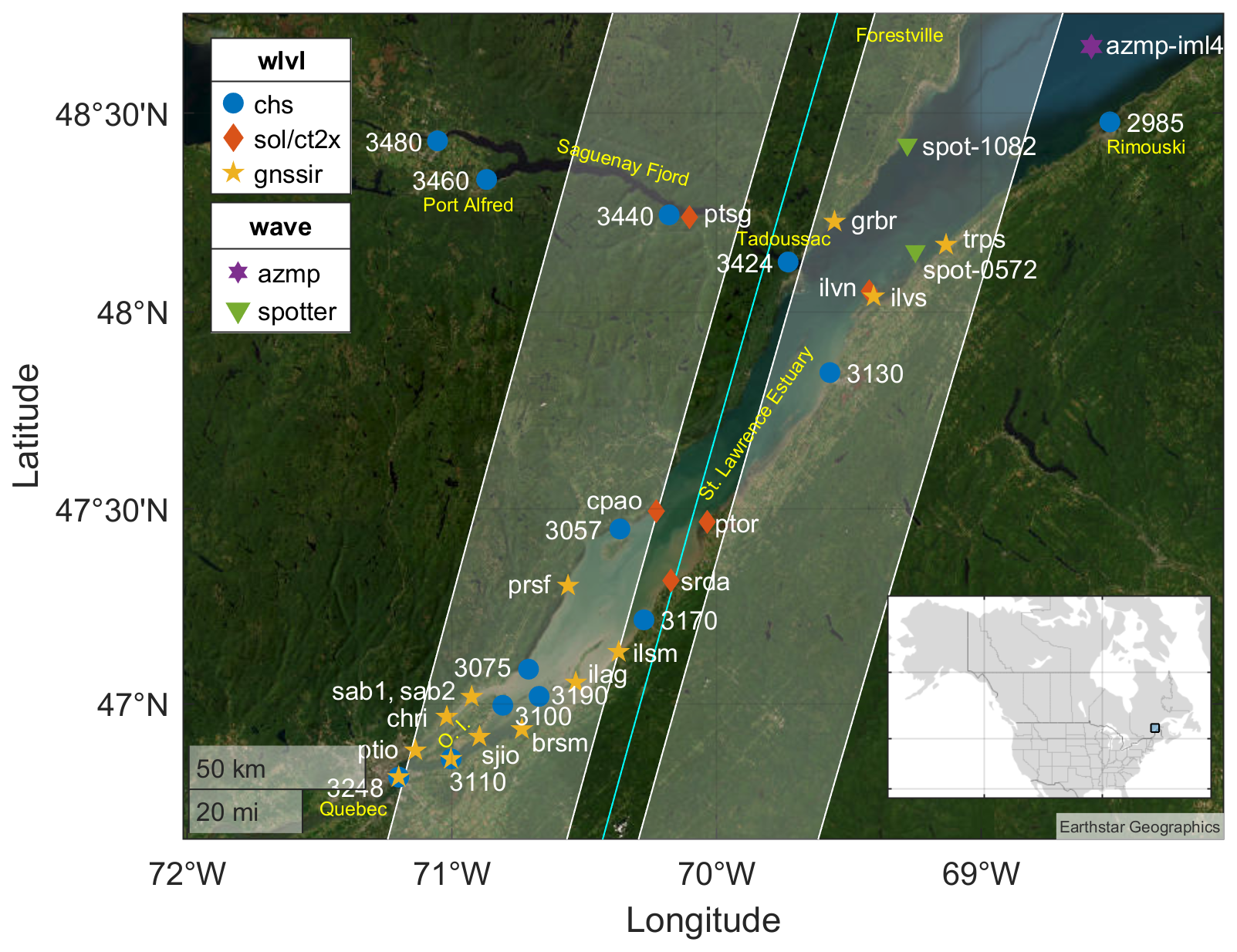
Figure 1SWOT Cal/Val orbit over the St. Lawrence Estuary and Saguenay Fjord, represented by two 50 km wide swaths (white) separated by a 20 km wide gap around nadir (cyan). Markers differentiate water level (wlvl) and wave stations by their sensor type (see Table A1 and main body text for more station details and definition of acronyms). Main location names are labeled in yellow. O.I. stands for Orleans Island (Île d'Orléans/I.O. in French).
The water level data was acquired using two types of sensors: pressure transducers (18) and GNSS-IR sensors (13). Their respective geographic coordinates are given in Table A1 together with their acquisition period, datum conversions, survey characteristics and associated errors. Table A1 also indicates whether the pressure data were corrected for water density. Further details on the included variables, their sampling frequency and units are provided in Table A2. The following subsections provide technical details on instrumentation, site configuration and data processing.
3.1.1 Pressure transducers
Water level data from 9 permanent tide gauges operated by CHS were downloaded from the Canadian Tides and Water Levels Data Archive (https://www.meds-sdmm.dfo-mpo.gc.ca/isdm-gdsi/twl-mne/index-eng.htm, last access: 23 September 2026). For each regular station, three independent water level sensors were co-located with a common data logger. The instrumentation consisted primarily of vented differential pressure transducers with built-in atmospheric pressure compensation, namely OTT PLS-L or OTT PLS 500 sensors deployed in freshwater, and OTT PLS-C sensors deployed in saline environments. Only Banc du Cap Brûlé (3075) and Baie-Sainte-Catherine (3424) were equipped with a combination of one FTS64 radar and two OTT PLS-C sensors. These data underwent routine data quality control by CHS (cf. Sect. 3.1.4) and were retrieved once their status had changed from preliminary to validated. The resulting minute-resolution water level corresponds to the mean of the three sensor measurements over each sampling interval, except when one sensor is unavailable or flagged as problematic, while no averaging is performed at radar stations. Overall, measured water levels at the CHS permanent stations have a total propagated uncertainty below 3 cm (2σ), except at Baie-Sainte-Catherine (3424), where it reaches 5 cm (2σ).
Additionally, 4 temporary tide gauges were installed by CHS between May/June and September 2023 to support this study. Each station was equipped with a Solinst Levelogger that measured absolute pressure, temperature, and conductivity, either mounted inside a pipe attached to a vertical structure (Fig. 2a), or fixed to a concrete block placed at the bottom of the river (Fig. 2b). At the L'Anse-Saint-Jean site (3440), 3 additional collocated OTT PLS-C vented pressure probes with conductivity cells were attached to the same concrete block; data from this triplet was later averaged into a single time series. Owing to the temporary nature of the installations and the use of sensors different from those at the permanent stations, the water level uncertainty at these sites is expected to be below 5 cm (2σ).
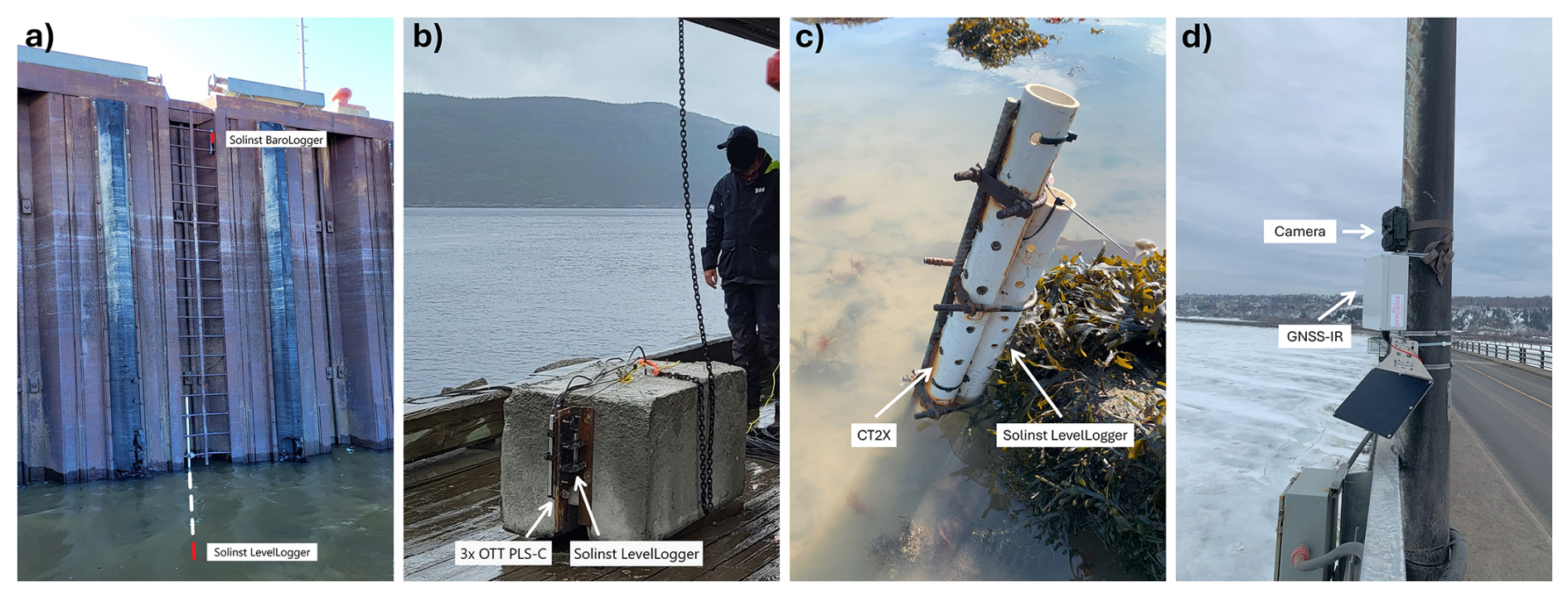
Figure 2Four types of installations for water level stations: (a) pipe mount with CHS Solinst sensors at Grosse-Île (3190); (b) concrete block with CHS Solinst and OTT PLS-C sensors at L'Anse-Saint-Jean (3440); (c) riverbed installations of Solinst and CT2X sensors at Cap-aux-Oies (cpao); (d) GNSS-IR sensor above water at Orleans Isl. bridge (ptio).
Five additional stations were installed nearshore after the loss of ice, between May and October 2023. Four of these stations were equipped with two sensors: one Solinst Levelogger measuring absolute pressure and temperature, and one Seametrics CT2X sensor measuring conductivity, temperature, salinity, total dissolved solids, and absolute pressure. The fifth station, at Isle-Verte (ilvn), was equiped with a single Solinst Levelogger. The sensors were placed inside perforated PVC pipes, which were then attached to metal rods hammered into the riverbed (Fig. 2c). For the five stations, the uncertainty is estimated to be less than 7 cm (1σ), with 7 cm representing the upper bound of the individual uncertainty estimates. The survey height error for each sensor is provided in Table A1; see Sect. 3.1.3 for details on the datum corrections and associated uncertainties.
Absolute pressure readings were barometrically compensated using collocated barometers from independent Solinst Barologgers installed above water, with an accuracy of ±0.05 kPa. The data from each sensor was converted to water levels using the equation for hydrostatic pressure, which reads
where h is the water column height above the sensor (m), P is the compensated pressure (kPa), ρ is water density (kg m−3) and g is the gravitational acceleration (m s−2). The derived water heights were then referenced to a common datum following a procedure described in Sect. 3.1.3.
In the estuarine transition zone, downstream of Orleans Island (O.I.; I.O. in French), water density oscillates with tides between freshwater and brackish water. Water density in Eq. (1) was computed using salinity and temperature data where available (Ruiz-Martinez, 2023); a constant value of 1000 kg m−3 was used otherwise. Both density-corrected and uncorrected data are provided in the dataset, along with temperature and salinity data, when available.
3.1.2 GNSS-IR sensors
Ground-based GNSS-IR antenna arrays (Purnell et al., 2021) were used to monitor water levels in the St. Lawrence Estuary. These sensors were chosen for their ease of installation (especially in wintertime) and for their potential to provide additional information about rough (icy or wavy) surface conditions (Purnell et al., 2024a). A total of 13 low-cost GNSS-IR sensors from Precipice Sensors Inc. were attached on poles or lampposts facing the water a few meters away from the shoreline (Fig. 2d). Each sensor contains four u-blox SAM-M10Q antenna modules that are mounted on ground planes and connected to a data logger. Most sensors were powered with batteries and connected to a solar panel, except for two sites with access to continuous power. Three sensors were equipped with a cell connection for real-time data transmission.
The GNSS-IR processing technique was based on Purnell et al. (2024b) and consisted of two key stages. First, Signal-to-Noise ratio (SNR) measurements were analyzed using a Lomb-Scargle Periodogram (LSP) to obtain an unevenly spaced time series of water level estimates (these estimates are referred to henceforth as arcs). Second, a moving-window spline-fitting technique was applied on the arcs to obtain a regularly spaced and smoothly varying time series of water levels. Tropospheric delay and height rate corrections were applied during the spline-fitting (Purnell et al., 2024b; Nikolaidou et al., 2020, 2023). Both the arcs and spline-fitted water levels are provided in this dataset. All GNSS-IR water levels were referenced to a common vertical datum, as described in Sect. 3.1.3.
GNSS-IR parameters that were previously shown to be useful for monitoring ice and wind speed (Purnell et al., 2024a) were calculated along with water level estimates as part of arcs processing stage. These parameters were calculated after applying an LSP and also a wavelet transform on SNR measurements. Certain parameters, including Confidence Level Retrieval (CLR) and Area Factor (AF) are taken from other literature (Kim et al., 2021; Song et al., 2022). The full list of parameters and their definition is provided in Table A2.
A time-varying estimate of the error in the spline-fitted GNSS-IR water levels was calculated. This error estimate refers to a one standard deviation error of the hourly water level nodes that were estimated during the spline fitting process. Refer to Purnell et al. (2024b) for more information about the water level nodes. The water level nodes and errors were estimated using the least squares algorithm called leastsq in the scipy Python library (Virtanen et al., 2020). On average, spline-fit errors ranged from 0.051 m (grbr) to 0.151 m (ptio) for the data presented here (see Table A1). More details about other sources of uncertainty in GNSS-IR data are discussed in Purnell et al. (2020).
3.1.3 Datum adjustments
Water levels were referenced to a common vertical datum, the static Canadian Geodetic Vertical Datum of 1928 (CGVD28, hybrid geoid model HTv2.0). CHS data are typically referenced to chart datum based on GPS-leveled water levels during installation and demobilization. They were converted from the chart datum to CGVD28 using factors listed in Table A1, provided by the solution from Canadian Spatial Reference System Precise Point Positioning (CSRS-PPP) at reference benchmarks taken by CHS. The remaining stations were referenced using real-time kinematic (RTK) GNSS corrections based on a Virtual Reference Station (VRS) network (either Can-Net or, when not available, Quebec’s Ministry of Natural Resources and Forests geodetic network), capable of centimeter-level accuracy. RTK-measured water levels taken near the sensors at different stages of the tide were used to reference pressure transducer data. A weighted average was applied on each group of RTK-point measurements based on the GNSS vertical accuracy (Table A1), with weights equal to the inverse of the vertical errors. The regularly-sampled sensor data was interpolated to the exact RTK timestamps before computing the transformation. In contrast, RTK-measured heights of the GNSS-IR sensors were used to convert reflector heights data into absolute water levels, instead of using direct water level measurements. In fact, direct RTK-measured and GNSS-IR derived water level comparisons were not always possible due to the difficulty of access to a representative open water point. Overall, the accuracy in absolute water levels is estimated to range between 0.01 and 0.07 m. Survey height errors are provided in Table A1 for all stations. Further validation details are provided in Sect. 5.
Different coordinate systems and tidal conventions are used in SWOT products and in the Canadian geodetic reference system (JPL D-109532, Revision A, 2025). SWOT water surface elevations (i.e. water levels) over continental waters are expressed relative to the mean-tide EGM08 geoid, while the associated position variables are provided in the International Terrestrial Reference Frame 2014 (ITRF2014) at the measurement epoch. To facilitate direct comparison between the in situ observations and SWOT water surface elevations, the following conversion procedure can be applied:
-
First, for observations referenced to CGVD28 using HTv2.0, the orthometric height is converted back to an ellipsoidal height using the HTv2.0 realization and reference epoch 1997.0 adopted for the dataset. The ellipsoidal height is obtained as , where H is the CGVD28 orthometric height and N is the HTv2.0 geoid undulation. This conversion can be performed with the Natural Resources Canada (NRCan) GPS⋅H tool (https://webapp.csrs-scrs.nrcan-rncan.gc.ca/geod/tools-outils/gpsh.php, last access: 23 September 2026).
-
The resulting ellipsoidal coordinates can then be transformed from NAD83(CSRS) epoch 1997.0 to ITRF2014 at a fixed epoch of 11 July 2023 (2023.5233) using the NRCan TRX tool (https://webapp.csrs-scrs.nrcan-rncan.gc.ca/geod/tools-outils/trx.php, last access: 23 September 2026). For consistency across the dataset, a fixed reference epoch of 11 July 2023 (2023.5233), corresponding to the end of the SWOT Calibration/Validation phase, was used for this transformation, rather than the individual measurement epochs. The vertical error associated with this fixed-epoch approximation is estimated to be on the order of 1 cm over the first three years of the SWOT mission (2023–2026), which is considered negligible relative to other sources of uncertainty associated with the in situ surveys. For applications requiring higher accuracy, conversion factors could instead be calculated for the specific date of each SWOT overpass.
-
Because conventional GNSS positioning generally provides coordinates in a conventional tide-free system, in which the permanent deformation associated with the solid Earth tide is not represented, this deformation, Δhpd, should subsequently be added to the resulting ellipsoidal heights before comparison with SWOT, following Eq. (11.7) of the SWOT User Handbook (JPL D-109532, Revision A, 2025), using the parameters specified therein, repeated below:
where h2=0.6078 is the Love number, m is the permanent tide-potential amplitude, and θlat is the latitude. The resulting ellipsoidal height is then expressed consistently with the reference ellipsoid used for SWOT water surface elevations.
-
To obtain a water surface elevation relative to the SWOT vertical reference, the geoid height provided in the SWOT High Rate (HR) products at the corresponding location should be subtracted from the corrected ellipsoidal height. These are already expressed in the mean-tide system; therefore, no additional mean-tide correction is required when the SWOT-provided EGM08 geoid height is used (version D or earlier). For this dataset, geoid values from 176 passes acquired over approximately one year during the Science orbit were extracted from the SWOT Level-2 KaRIn High Rate Raster Product, Version D. These successive passes provide repeated but spatially shifting coverage of the study area and were averaged to produce a spatial map of mean geoid height. The geoid height at each gauge location was then obtained by extracting the value from the nearest 100 m grid cell of this map.
The complete conversion from the Canadian vertical reference system to the vertical reference used by SWOT can be expressed as:
where HCGVD28 is the water surface elevation relative to CGVD28, NHTv2.0 is the geoid undulation from the HTv2.0 model used to convert the CGVD28 orthometric height to an ellipsoidal height, ΔhTRX is the ellipsoidal-height change resulting from the transformation from NAD83(CSRS) at epoch 1997.0 to ITRF2014 at epoch 2023.5233, Δhpd is the permanent deformation correction given by Eq. (11.7) of the SWOT User Handbook (JPL D-109532, Revision A, 2025), and NSWOT is the mean-tide geoid height provided by the SWOT geoid variable at the corresponding location. The resulting HSWOT is the water surface elevation relative to the mean-tide EGM08 geoid used by SWOT. The workflow is summarized in Table 1, and the corresponding conversion factors are provided in Table A1 for each station.
Table 1Workflow for converting in situ water level observations from the Canadian geodetic reference system to the vertical reference used by SWOT.

3.1.4 Quality control of water level data
Quality control performed by CHS at their permanent stations consisted in (1) comparing measured water levels against minimum and maximum thresholds defined at each station, (2) assessing the differences between water levels measured by collocated sensors when possible, (3) comparing the measured water levels against tide forecasts when available, and (4) manual verification by an expert on a daily basis. The four temporary stations deployed by CHS underwent manual quality control only, as neither collocated sensors nor forecasts were available, with the exception of L'Anse-Saint-Jean (3440) where both Solinst and OTT PLS-C sensors were installed.
Quality control measures for the remaining pressure transducers were mainly based on the temperature and/or salinity data measured by the sensors. Sudden changes or erroneous values in temperature or salinity, often related to the sensor being above water, were flagged and the corresponding water levels disregarded. The procedure for detecting erroneous values of temperature or salinity is as follows. First, temperature values lower than 0 or higher than 100 °C, as well as salinity values lower than 0.5 or higher than 100 PSU, were disregarded. These thresholds are chosen considering that the pressure and conductivity sensors were installed from spring to fall in the brackish waters of the estuarine transition zone. Additional outliers were detected by calculating the scaled Median Absolute Deviation (MAD) in a moving window of 14 d, corresponding approximately to the neap-spring tidal period. If the absolute difference between a point and the median value in the window was greater than five, then the point was considered to be an outlier and removed. The results from applying this algorithm on salinity data are presented in Fig. 3.
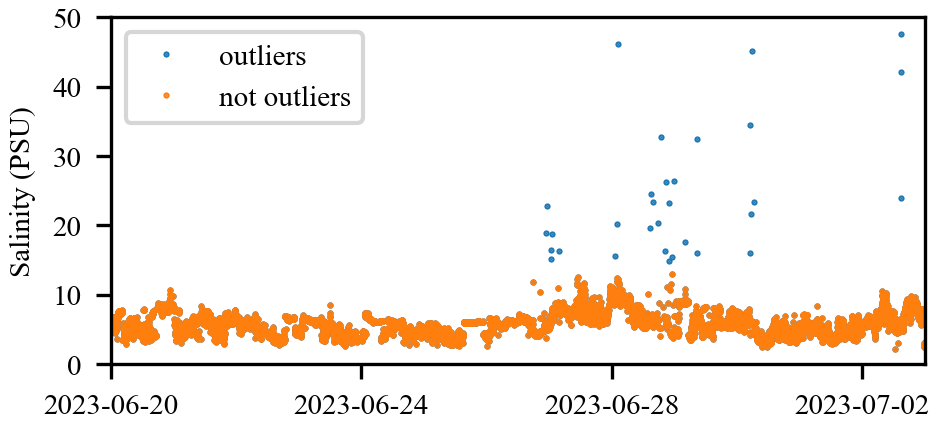
Figure 3An example showing outliers detected in the salinity data at the Petit-Saguenay station (ptsg).
Quality control measures were applied during both stages of the GNSS-IR processing. To produce the arcs, threshold-based criteria were applied so that any water level estimate obtained from an LSP with a peak-to-noise ratio or CLR smaller than 3 was disregarded. During the spline-fitting stage, large errors often occurred when there was a large gap in time between water level estimates. Therefore, any water level node with a standard deviation error greater than one meter was disregarded. The spline-fitted water level data also contains a “ground flag” that is raised whenever the measured levels are near or below the local bed elevation. This flag was only raised at sites where the shoreline recedes sufficiently during low tide to expose extensive intertidal flats, and where RTK-GNSS measurements of the river bed in front of the sensor were taken. Under these conditions, the sensor may measure the exposed bed surface rather than the water level, resulting in a truncated or nearly constant water level signal until the rising tide inundates the area again. At other sites where the river bed was not surveyed with RTK-GNSS, similar truncation may occur during exceptionally low tides but cannot be identified with the same confidence.
3.2 Wave data and instrumentation
To refine temporal observations of water surface conditions, we supplemented water level measurements with wave data that were recorded by two types of moored directional wave buoys: firstly, by the Atlantic Zone Monitoring Program (AZMP) IML-4 Viking platform built by the Canadian company MTE Instruments, located amidst the St. Lawrence Estuary, between Rimouski and Forestville (Fig. 1, purple star); secondly, by two commercial Sofar Ocean Spotter buoys (hereafter Spotter) that were deployed at Les Escousmins and Trois-Pistoles (Fig. 1, green triangles) during the SWOT Cal/Val phase. Figure 4 shows these two types of buoys, comparing shapes, weights, dimensions, auxiliary systems, and wave sensor position.

Figure 4Sketches of the AZMP (left) and Spotter (right) wave buoy apparatus. Note: the respective sizes of the two instruments are not shown to scale.
The three buoys were deployed in contrasting locations. The Rimouski AZMP IML-4 buoy floated far offshore, with a water depth of 335 m beneath it. Similarly, the Les Escousmins SPOT-1082 buoy was located in deep waters, with a water depth of 200 m, but closer to shore. In contrast, the Trois-Pistoles SPOT-0572 buoy was operating in very shallow waters, with a water depth of 4 m, near the coast, but unfortunately stopped recording waves five days after start-up due to a faulty battery connector. We still provide the data collected up to the time of cessation. Details regarding the location, operating dates, GPS coordinates and water depth for each wave buoy are given in Table A3.
Each buoy yields short-term (ST) time series of surface motions, specifically providing 4.0 Hz linear acceleration data for the AZMP model and 2.5 Hz displacement data for the Spotter. Subsequently, long-term (LT) time series of wave bulk parameters are derived at 30 min intervals using well-established spectral methods.
3.2.1 The AZMP IML-4 platform
The IML-4 is a multidisciplinary platform that forms part of the AZMP by Fisheries and Oceans Canada (DFO), a network of seven similar platforms gathering extensive physical and biogeochemical data at a high rate in the St. Lawrence Estuary and Gulf (cf. Sect. 7.3). These tailor-made buoys conceived and developped by DFO and MTE Instruments operate exclusively during the ice-free season, typically from May to October. With their diameter of 2.24 m and height of 4.51 m, they are significantly larger than some compact-sized (40–70 cm, 7–30 kg) and medium-duty (70–150 cm, 50–250 kg) commercial standards such as the Sofar Spotter, Datawell Waverider series, NextSens CB series, and Triaxys products.
The AZMP buoys carry a wave-monitoring module positioned 20 cm above the still-water level, which tracks the wave field using a 4.0 Hz SCC1300-D02 3-axis accelerometer component. The module follows the standard AZMP sampling protocol, in which surface motions are sampled for 10 min bursts every 15 min, resulting in a 5 min gap between successive records. This sampling strategy is used across all sites to manage shared computing resources among onboard sensors, thereby limiting the data volume allocated for wave monitoring. Wind data were collected by an onboard Vaisala Ultrasonic WMT700 anemometer. Buoy heading and gyroscopic measurements were obtained from an external GPS and Rion-Tech CDM260B compas mounted externally to the wave module.
All additional data collected in conjunction with the wave module was sampled only once every half hour, including GPS and compass readings. Hence, it is important to note that acceleration data are likely to be biased towards trends or sporadic fluctuations caused by rolling, pitching, or tilting, due to the inability to account for gyroscopic measurements at the acceleration sampling rate. Such trends or fluctuations are perceived as steady or slowly evolving imbalances caused, for example, by biofouling, tidal flows, or slowly varying surface currents dragging the buoy out of its position of equilibrium. During the validation of the wave data, we noticed that the absolute mean of the compass readings for rolling and pitching was less than 1°, except for a few instances where it reached or exceeded 3°, under strong wind conditions. Although these unrectified biases are generally small, we acknowledge that this absence of high-rate gyroscopic readings may degrade the accuracy of acceleration data. To address this limitation, we flag time series showing significant mean shifts during the quality control procedure (see Table 2, test 4.12). Despite the same limitation when accounting for the buoy's heading, we noticed during wave data validation that correcting for its heading is crucial for accurate wave directional moment estimations. By considering the lower rate 30 min GPS heading as a mean value for correction, we obtained interpretable values for wave provenance and spreading, as shown later in Sect. 5.2.
IML-4 post-acquisition processing was performed in order to provide the users with a faithful description of ambient wave conditions in the SLS. We recall that IML-4 supplies a rich variety of data alongside wave monitoring, which can be accessed in the datasets that we promote. This includes environmental conditions and auxiliary physical quantities that are available every 30 min: acoustic Doppler current profiler (ADCP) measurements of near-surface water velocity (bin #1), conductivity-temperature-depth (CTD) observations of the water body, and atmospheric relative humidity, pressure and temperature.
We carried out a comprehensive spectral analysis of the linear acceleration to describe dominant scales and the provenance of surface motions evolving under wind forcing. We used a fifth-order high-pass Butterworth filter to remove low-frequency motions that unlikely corresponds to the orbital motion of waves, such as horizontal displacements caused by tidal currents, wind blowing against the buoy, or Stokes drift. For filtering, a cutoff period pc≈11.3 s equivalent to a wavelength of 200 m for deep-water linear waves is chosen. Such scale embeds the most significant part of wave spectrum related to surface gravity waves. It also filters out slow horizontal oscillations that are allowed by the mooring cable, which is the most important source of signal contamination. Subsequently, bulk wave parameters were calculated from the average cross-spectral density of paired, consecutive 10 min data bursts recorded every 15 min, yielding an effective temporal resolution of 30 min. Lastly, the quality control of ST and LT time series was performed (see Sect. 3.2.3).
3.2.2 Spotter wave buoys
Additional Spotter buoys deployed during SWOT's Cal/Val fast-sampling and early Science phases were operational from late May to mid August 2023, with the aim to increase and densify wave measurements under the SWOT Cal/Val orbit. Surface displacements of the water body were measured through a GPS-based approach (Raghukumar et al., 2019), leading to a continuous acquisition at 2.5 Hz, and resolving the 0.029 to 0.8 Hz frequency bands. Similar to IML-4, spectral analysis was used to quantify wave field characteristics such as height, period, provenance (angle relative to its sources) and spreading, derived from high-pass filtered wave spectra. Validation results are presented in Sect. 5.2.
3.2.3 Quality control of wave data
For each ST time series of surface motions and the corresponding LT time series of wave parameters, a quality flag is assigned, consisting of a primary code and a secondary code. The primary code is determined based on the nature of quality control, while the secondary code indicates the reliability in the event of hardware failure and anomalous or severe gradients in environmental conditions that could affect the buoy’s measurements of wave conditions.
The quality control is assessed following standard testing procedures described in Bushnell (2019), categorizing data as “1” (good), “3” (suspect), “4” (fail) or “9” (missing). The assigned secondary code corresponds to the test number that has served for classifying the data as faulty or suspect. For AZMP buoys, we provide an additional quality-control flag indicating whether horizontal acceleration could not be corrected for buoy heading due to the absence of readings. In such cases, we assign primary and secondary quality codes of “4.NH” for horizontal acceleration. We continue to provide horizontal acceleration, but users should note that the wave processing cannot proceed further beyond this point, and therefore directional wave parameters cannot be calculated. Otherwise, data are considered physically reliable if all tests are satisfied. Finally, if a LT time series of wave parameters was calculated using a suspect or flawed ST time series with quality codes of “4.9”, “4.12” or “4.NH”, then the derived bulk wave parameters may not accurately reflect real-world wave conditions due to insufficient, scarce data or the lack of rectification for tilting, rolling, pitching and heading.
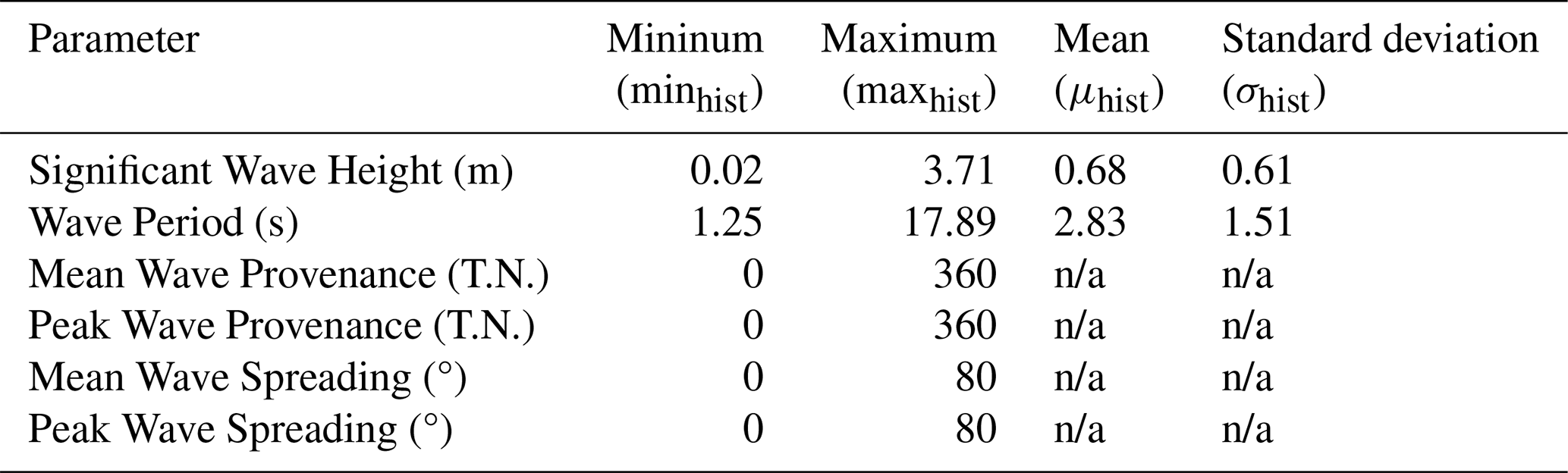
As erroneous or erratic measures can be detected by multiple tests, we first tested for faulty data, then for suspect ones. The secondary code is established by first checking for data lying outside the operator-defined range, then we flag missing or flattened data, which may indicate measurement error. Next, we looked for data with prominent mean shifts, indicating that the buoy has shifted relative to its equilibrium position which we could not account for during post-processing. Finally, we analyzed whether there are acute rates of change in the data, or if they fall outside the statistically expected range based on historical wave data. Table 2 presents the sequence of tests used to establish the primary and secondary quality codes for ST and LT time series. Statistical ranges were calculated from data acquired by the IML-4 station since 2014, available from St. Lawrence Global Observatory (SLGO) at https://www.ogsl.ca/en/home-slgo/ (last access: 21 September 2026). The resulting set of statistical computations is summarized in Table 3, which include minimum, maximum, mean and standard deviation values for each wave parameters, with three considerations to note. Firstly, the minimum significant wave height is set to a small non-null value, as a zero-value could imply either a perfectly still surface or sensor failure. Thus, to avoid ambiguity it was set arbitrarily to 0.02 m. Secondly, the minimum wave period was determined from the inverse of the Nyquist frequency, using the lowest sampling frequency fs of the two buoys, yielding minperiod=1.25 s. Third, it is unlikely that the maximum value for wave spreading is 90°, as this would suggest an equal distribution of the wavefield in all directions; therefore, a value of 80° was established.
Table 2Primary and secondary quality codes for wave buoy ST times series of surface displacements or accelerations and their derived spectral variables, as well as for LT time series of wave parameters.

Table 3Historical lower and upper bounds for every wave parameters, either defined by operators or statistically derived from historical wind and wave data recorded by the IML-4 station from 2014 to 2024, inclusive. T.N. stands for True North. n/a – not applicable
This section provides an overview of the datasets, detailing their temporal coverage, content, and the formats associated with each processing level.
4.1 Temporal coverage
A summary of the available water level and wave data at each station is provided in Fig. 5. While the SWOT Cal/Val period is covered by a denser network of stations, several sensors remained in place during the SWOT Science phase, thus allowing for a continued validation of the satellite observations during the two mission phases. Stations that have since been dismantled are indicated by an X marker and will no longer contribute to future dataset updates.

Figure 5Timelines of available and processed wave (yellow) and water level data (blue: St. Lawrence Estuary; orange: Saguenay Fjord) for each station and sensor, ordered by longitude. Vertical dashed lines delimit the SWOT Cal/Val period. X markers indicate stations that have been dismantled and will no longer be updated.
4.2 Files and format
Three water level and wave data levels are included in the dataset, where relevant:
-
Level 0 (“l0”): Raw files exported directly from the sensors without further processing.
-
Level 1 (“l1”): Converted files, with uncorrected or unsmoothed variables. Only basic quality control is applied at this stage.
-
Level 2 (“l2”): Files with global datum adjustments, corrections and quality control applied. These files are considered to be ready for scientific analysis.
4.2.1 Water level data
This section describes each water level data type and format contained in this dataset. The data folders are structured by station name, sensor type or provider, and processing level. File naming follows the convention “[4-character ID]_[sensor type or provider]_[level].csv”, where the station ID is provided in Table A1, and the sensor type or provider is one of “baro”, “sol”, “ct2x”, “gnssir”, or “chs”, which stand for Solinst Barometer, Solinst Levelogger, Seametrics CT2X, GNSS-IR, and CHS (Solinst or OTT PLS-C), respectively. Although most of the CHS data was acquired using Solinst sensors, we differentiate them from the Solinst data that was acquired by our team due to differences in the level of processing and quality control applied.
For each sensor, CSV files are provided following a definition of the data levels as follows:
-
Solinst Barometer (“baro”):
-
Level 0: corresponds to atmospheric pressure and temperature readings.
-
Level 1: no data are provided at this level.
-
Level 2: no data are provided at this level.
-
-
Solinst Levelogger (“sol”):
-
Level 0: corresponds to uncorrected water level and temperature readings.
-
Level 1: corresponds to barometrically compensated heights, in the sensor (arbitrary) reference, along with temperature data. No density corrections are applied during data conversion.
-
Level 2: corresponds to water levels referenced to a common vertical datum (CGVD28). The temperature data is also included and used to detect and remove outliers from the water level data.
-
-
Seametrics CT2X sensors (“ct2x”):
-
Level 0: includes absolute pressure, temperature, conductivity, salinity, and total dissolved solids (TDS) readings.
-
Level 1: includes barometrically compensated and density-corrected heights, in the sensor (arbitrary) reference.
-
Level 2: includes water levels referenced to a common vertical datum (CGVD28). The temperature and salinity data is also included and used to detect and remove outliers from the water level data.
-
-
GNSS-IR data (“gnssir”):
-
Level 0: no data are provided at this level.
-
Level 1: rawest, irregularly sampled water level data available after converting the satellite arcs into water level estimates, but before spline-averaging the noisy data. The other GNSS-IR parameters (SP, PTN, AF, etc.) are also included as separate columns in the same files (see definitions in Table A2). Daily files are provided and labeled using the date format “yymmdd_24h”.
-
Level 2: corresponds to smoothed (spline-fitted), regularly sampled water levels and associated uncertainty, referenced to a common vertical datum (CGVD28).
-
-
CHS data (“chs”):
-
Level 0: at 4 temporary stations only (3130, 3170, 3190, 3440), files associated with the Solinst sensors include uncorrected water level, temperature and salinity readings. For one station (3440), a separate OTT PLS-C file is included that has the same variables in triplicate along with quality flags. No data are provided at this level for permanent CHS station.
-
Level 1: at all CHS stations, compensated and quality controlled water levels for both Solinst and OTT PLS-C sensors, referenced to the local chart datum. Density corrections were applied during data conversion.
-
Level 2: at all CHS stations, this includes the same quality-controlled data as in Level 1, but converted to a common vertical datum (CGVD28). At the 4 temporary CHS stations only, additional fields are provided for temperature and salinity.
-
The data temporal sampling along with the full list of variables and their definition are provided in Table A2 for each data type and for processing levels 1 and 2.
4.2.2 Wave data
We organize the data for each wave buoy into distinct levels, analogous to water levels. For each buoy, year, and data level, we produced NetCDF files that facilitate simple and efficient access to all the variables and their attributes for a particular season and locations. For each variable, attributes comprise a concise description, units, and the related quality flag and code time series. One should be aware that quality control is not offered for ancillary variables, as the primary focus is on wave data.
The data folders are structured by buoy type (either “azmp” or “spot”), station name, and processing level. The file names follow a straightforward convention that combines the buoy type and ID (as listed in Table A3), the processing level, the data type, and the year the data was collected. The format is as follows: “[buoy_ID]_[level]_[type]_[year].nc”. The wave buoy datasets are organized into three levels that increase upon the degree of processing:
-
AZMP platform (“azmp”):
-
Level 0, Type “accelerations”: Contains all 10 min acceleration time series, sampled at 4.0 Hz and acquired every 15 min, along with the corresponding ST quality control flag.
-
Level 0, Type “auxiliaryvariables”: Consists of physical auxiliary variables recorded by the platform. Eulerian sea water velocity and direction measured by acoustic Doppler current profiler (bin #1), atmospheric relative humidity, pressure and temperature at sea level, buoy geoposition, orientation and course, and CTD measurements. Wind data is also provided at this stage.
-
Level 1, Type “wavespectra”: Comprises the auto-,co-, and quad-spectral densities, as well as the first and second directional moments. These spectral values were calculated every 30 min based on the previous two 15 min level 0 records. The quality control is inherited directly from ST level 0 records.
-
Level 2, Type “waveparameters”: Includes wave parameters computationally integrated from level 1 wave spectra, over 30 min intervals. Each wave parameter is accompanied with an LT quality code or inherits an ST quality code if the calculation was done prior with an ST time series flagged “4.9”, “4.12” or “4.NH” (see Sect. 3.2.3). The bulk wave parameters consist of significant wave height hm0, wave energy period Tm−10, mean wave period Tm01, mean zero-crossing period Tm02, mean and peak wave provenance θm and θp, mean and peak wave directional spreading σm and σp, respectively. The peak frequency and its associated peak wavenumber calculated using the dispersion relation for linear waves are also comprised.
-
-
Sofar Spotter wave buoy (“spot”):
-
Level 0, Type “displacements”: Provides the complete time series of displacements, measured at 2.5 Hz, and resampled to 30 min intervals. Quality codes for each segment are provided, along with the corresponding longitude and latitude of the buoy.
-
Level 1, Type “wavespectra”: Provides cross-spectral matrices and directional moments computed each 30 minutes from level 0 data. Quality codes are ST level 0 replicas.
-
Level 2, Type “waveparameters”: Includes wave parameters as those described above for AZMP buoys, along with an LT quality code or an inherited ST one.
-
This section presents the validation results for water level and wave data, including sensor intercomparisons, computed corrections, and key insights into the observed surface properties and environmental conditions of the St. Lawrence Estuary and Saguenay Fjord.
5.1 Water level data validation
5.1.1 Pressure gauge comparisons
A comparison of water level time series obtained from three different sensors at two nearby stations in the Saguenay Fjord (L'Anse-Saint-Jean and Petit-Saguenay) is presented in Fig. 6. As a reference, time series from downstream and upstream stations are also included to illustrate how tides are evolving between Baie-Sainte-Catherine (3424), located at the fjord entrance, and Port-Alfred (3460), about 95 km upstream. Midway between these stations, at L'Anse-Saint-Jean (3440), both CHS Solinst Levelogger and OTT PLS-C sensor data were highly consistent with each other, showing only very slight differences, with root-mean-squared and maximum absolute differences of 0.008 and 0.08 m, respectively, and a mean bias of 0.004 m for the entire record length. Similarly, comparisons between CHS data at L'Anse-Saint-Jean (3440) and Solinst levelogger data at Petit-Saguenay (ptsg), located 5 km apart, show root-mean-squared differences (RMSD) of 0.045 m and a bias of 0.005 m. These differences are mainly associated with the Petit-Saguenay sensor drying out at low tide (see Fig. 6, bottom panel). When put in relation with downstream and upstream stations at Baie-Sainte-Catherine and Port-Alfred, the standing-wave character of the tides in the Saguenay fjord clearly stands out. While tidal signals are almost perfectly in phase throughout the entire fjord length, they are amplified landward from 5.1 to 6.3 m in range during spring tide (grey-shaded area in Fig. 6).
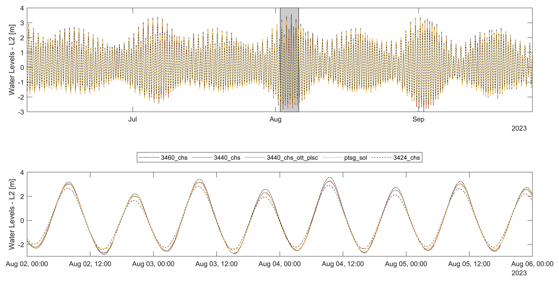
Figure 6Quality-controlled level-2 water levels (CGVD28) in the Saguenay Fjord at L'Anse-Saint-Jean (3440; CHS Solinst and OTT PLS-C sensors) and Petit-Saguenay (ptsg; Solinst sensor). Dash-dotted and dashed lines show the water levels at Port-Alfred (3460) and Baie-Sainte-Catherine (3424) upstream and downstream stations, respectively, separated by about 95 km. The grey-shaded area in top panel corresponds to the zoomed-in period in bottom panel.
The Seametrics CT2X sensor at Petit-Saguenay was intentionally left out of the analysis as it was showing a systematic bias compared to other gauges in the Saguenay Fjord. Even more so, the observed water levels were often falling outside the limits naturally imposed by the two boundary gauges at Baie-Sainte-Catherine (at the fjord entrance) and Port-Alfred (upstream). Assuming that the tide is being amplified from downstream to upstream and that mid-fjord stations were all in concordance except the CT2X one, it was chosen to disregard data from this sensor in Fig. 6. However, CT2X data were not removed from the database as they include relevant salinity and temperature information, as discussed in the next subsection.
5.1.2 Density corrections
In the Saguenay Fjord and in the St. Lawrence estuarine transition zone (downstream of Orleans Island), water density variations can be observed during the tidal cycle. As a result, differences in the estimated water levels can exceed one decimeter if not adjusted for density, due to the large tidal ranges in this area, reaching up to 7 m. In fact, density directly influence the calculated height of water above the sensor, mostly around high tide, when saline waters enter the estuary and when the water column is the deepest. While density corrections assume that the salinity and temperature measured at the sensor depth are representative of the water column, this may be only valid in shallow waters and less so as water depth increases. Nevertheless, the estimated effect of density on water levels is captured in Fig. 7 and further analyzed in Table 4.
Given that conditions oscillate between saltwater and freshwater as a function of the incoming tide, errors mostly occurred around high tide when a peak in salinity was reached, creating an apparent bias in the data, as shown in Table 4. While on average the error is comparable to the survey height accuracy (cf. Table A1), maximum differences (around high tide) can amount to up to 0.155 m (ptsg) based on comparisons of the CT2X L1 non-corrected heights and density-corrected heights. Figure 7 illustrates an example of these differences at Saint-Roch-des-Aulnaies (srda) located in the St. Lawrence estuarine transition zone. Density corrections associated with salinity and temperature variations show variability at both the semi-diurnal and neap-spring tidal scales. Further monthly variability is observed, likely linked to the seasonal cycle in river flow.
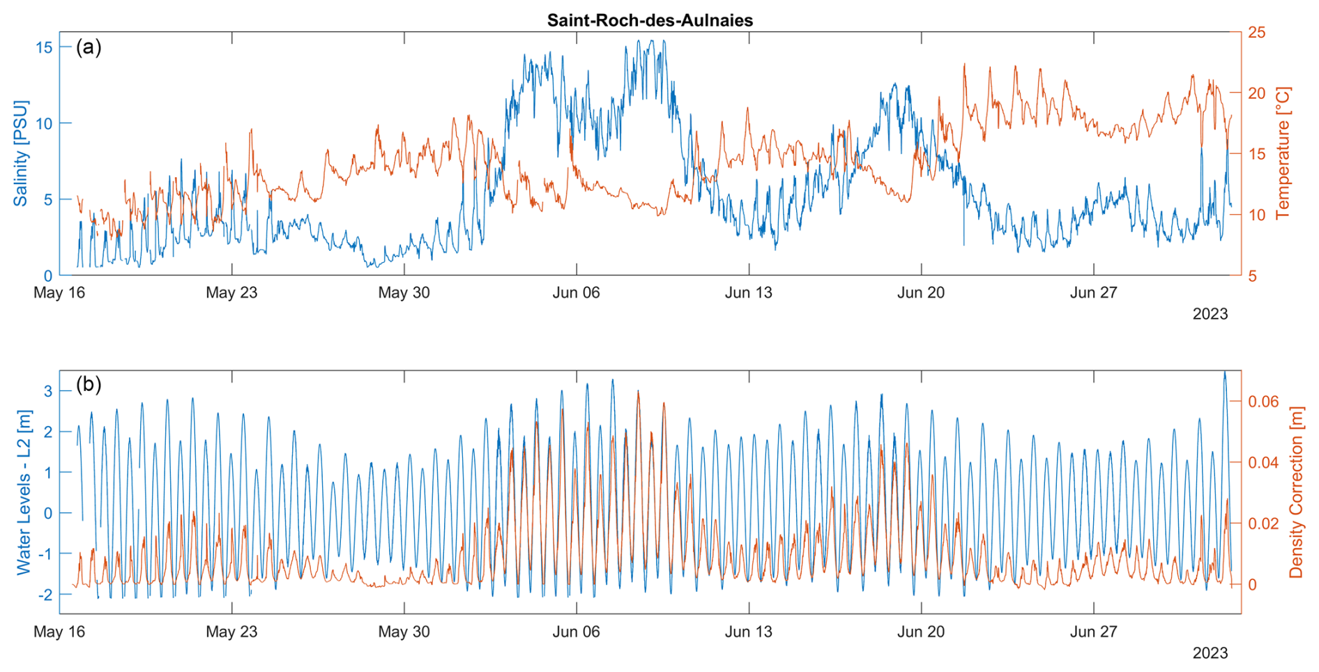
Figure 7Seametrics CT2X sensor data at Saint-Roch-des-Aulnaies (srda): (a) Salinity and temperature time series; (b) Level-2 water levels with corresponding density corrections.
Table 4Comparison between non-corrected and density-corrected heights from Seametrics CT2X Level 1 data. Metrics include root-mean-squared difference (RMSD), mean difference, maximum absolute difference, and the number of points at each sensor location.

In Table 5, a comparison between collocated Solinst Leveloggers and Seametrics CT2X sensors is provided, using both non-corrected and density-corrected water levels from the CT2X sensors. “No density correction” refers to L1 data that were datum-adjusted using coefficients provided in Table A1 but with minimal quality control (leading to more data points). “Density-corrected” entries refer to L2 water levels that have undergone quality control and are based on the density-corrected CT2X data. Note that in both cases, no density corrections were applied to the Solinst data, as salinity was only measured by the CT2X sensors and started behaving erratically after a few weeks or months after deployment, leaving the salinity records incomplete (see Fig. 5). This table should be looked at in conjunction with Table A1 where the number of survey points used for each sensor is presented. In general, less survey points were used for CT2X sensors because of sensor malfunctioning after a certain period of recording. As a result, CT2X records are generally shorter, they were referenced using less surveying points (since some of them were taken at the end of the deployments), and they show larger differences with nearby official CHS tide gauges. Overall, we consider these sensors less reliable; nevertheless, they provide information on the error made by neglecting density variations. In fact, the various error metrics shown in Table 5 tend to degrade when density-corrections are applied to the CT2X data, as they depart from the non-density-corrected Solinst data. A few centimeters difference can be observed on average beween non-corrected and density-corrected RMSD, with increasing biases and maximum absolute differences between the sensors.
Table 5Comparison between Solinst Levelogger and Seametrics CT2X sensors, without and with density-corrected CT2X water levels. Metrics include root-mean-squared difference (RMSD), mean difference, maximum absolute difference, and the number of matching points used for comparisons between the two sensors, for each location.

5.1.3 GNSS-IR – tide gauge comparisons
Water levels from collocated pressure gauges and GNSS-IR sensors closely match at the sites Saint-Laurent I.O. (3110) and Vieux-Québec (3248) (Table 6). At Saint-Laurent I.O., the RMSD between the (level 2) GNSS-IR and pressure-gauge-derived water levels is 0.0696 m from the period from 17 March 2023 to 23 May 2024 and the mean offset between the two water level time series (i.e. GNSS-IR minus tide gauge heights) is −0.0015 m. Furthermore, comparing GNSS-IR and pressure gauge water levels at Vieux-Québec for the time period from 20 March 2023 to 12 May 2024 results in an RMSD of 0.1017 m and a mean offset of −0.0339 m. GNSS-IR sensors and antennas differ between sites, which partially account for performance variability with site. A comparison between GNSS-IR water levels – both arcs (level 1) and spline-fitted (level 2) – and a collocated pressure transducer is shown in Fig. 8. The largest differences between CHS and GNSS-IR level 2 data were observed around high and low tides and likely arise from imprecision of the spline-fitting procedure around tidal extremas (Purnell et al., 2024b).
Table 6Comparison between GNSS-IR sensors and CHS tide gauges (Level 2). Metrics include root-mean-squared difference (RMSD), mean difference, maximum absolute difference, and the number of points at each sensor location.

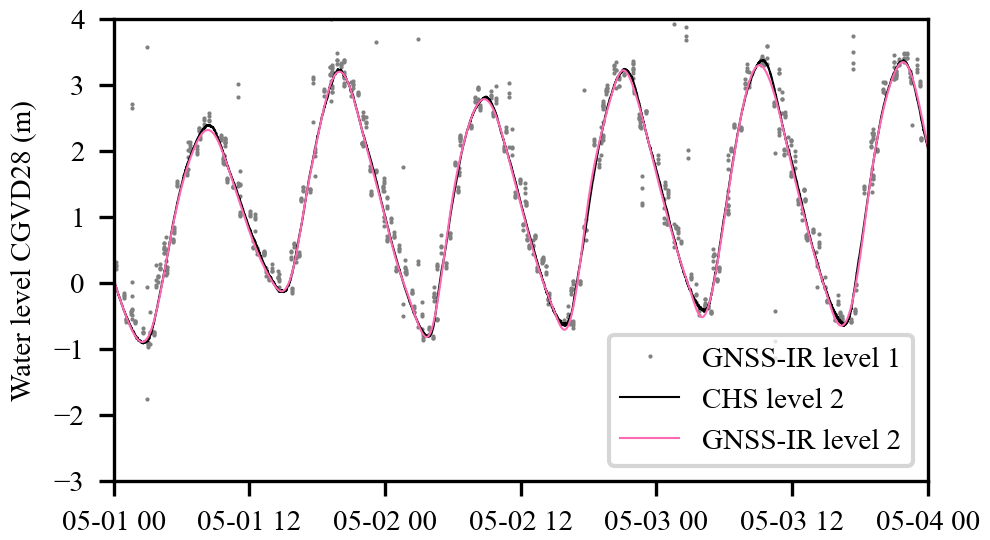
Figure 8Water levels in the St. Lawrence fluvial estuary at Saint-Laurent I.O. (3110) obtained from collocated tide gauge and GNSS-IR sensor. For the GNSS-IR sensor, both arcs (level 1) and spline-fitted water levels (level 2) are shown.
For consistency, all of the level 2 GNSS-IR water level time series were levelled to the CGVD28 datum using RTK measurements of the sensors themselves. At the Vieux Québec and Saint-Laurent I.O. sites, the water levels could also be levelled by using the pressure gauges. In this case, the RMSE between the GNSS-IR and pressure gauge water levels remains nearly unchanged at Saint-Laurent I.O. (0.06955 m) and reduces to 0.0959 m at Vieux-Québec. It would also be possible to level the GNSS-IR water levels using RTK measurements of water levels, however this is only possible at sites where overlapping measurements exist. Furthermore, direct RTK measurements of water levels taken in front of the GNSS-IR sensors are affected by wave conditions and can depart from water levels retrieved using GNSS-IR data across the instrument’s footprint. Therefore, no further adjustments were made.
5.1.4 Intertidal topography
In some areas along the St. Lawrence Estuary, extensive floodplains can be revealed at low tide. The associated intertidal topography is captured by some of the GNSS-IR sensors and flagged accordingly (only where RTK-GNSS measurements of the river bed are available), while low tides at other pressure sensors appear truncated. In the latter case, the recorded barometrically-compensated (L1) water levels under dry conditions are close to zero or become negative, with correspondingly abnormal (air) temperatures flagged during quality control.
Figure 9 illustrates water levels at Isle-Verte taken from two sensors: a Solinst Levelogger located on the North shore (ilvn_sol) and a GNSS-IR sensor positioned on the South shore (ilvs_gnssir). While the pressure sensor dried out during the lowest low tides and those segments were removed during quality control (as confirmed by comparing L1 and L2 Solinst data, not shown), the GNSS-IR sensor consistently showed truncated low-water levels, reflecting the extensive intertidal flats that border the narrow South shore channel at Isle-Verte. In this case, the ground flag was activated. However, these observations of the intertidal topography still suffer from some inaccuracies, as these points take part in the spline-interpolation procedure used to produce the water level time series, distorting the lower water levels before hitting the ground. Furthermore, given the footprint of the GNSS-IR (Fig. 9a), as the water recedes, one can suppose that only a portion of the observation points happen to be over dry topography, while the rest correspond to the water surface. This explains the observed variability in heights of the ground points in Fig. 9b. Nevertheless, comparisons of the ground-flagged elevations with SWOT observations during low tide could be conducted in a future study to assess the potential of SWOT in mapping intertidal topography, as demonstrated by Salameh et al. (2024).
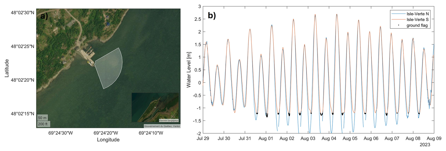
Figure 9(a) GNSS-IR footprint at Isle-Verte S (ilvs); (b) Water levels at Isle-Verte from Solinst Levelogger (ilvn_sol) on the North shore (blue line) and GNSS-IR sensor (ilvs_gnssir) on the South shore (red line) showing observed dry or partially dry topography (ground flag, black dots).
Further insights into tidal dynamics is revealed in Fig. 9, relating to tidal distortion in shallow water. While both sensors on the North and South shore of Isle-Verte present highly synchronized high waters, the low waters on the South shore (shallower) occur later than on the North shore (deeper). This leads to more abrupt rising tides and longer falling tides, a tidal asymmetry that typically translates into larger amplitudes of the shallow water tides (e.g. M4).
5.1.5 Longitudinal slopes
In tidal rivers and estuaries, water levels and hydraulic gradients exhibit spatial and temporal variability, ranging from gradual changes driven by the long-wave nature of tides to abrupt shifts induced by local topography or wind effects. These variations occur both in the cross- and along-channel directions (Hopkinson et al., 2011). While such gradients are often linked to river discharge, they are also influenced by processes including reversing tidal flow, Stokes drift compensation flow, neap-spring storage effects, secondary circulation, and differential water level setups within channel networks (Matte et al., 2019; Moftakhari et al., 2016; Sassi et al., 2011). Despite these complicating factors, understanding how the spatiotemporal dynamics of water surface slopes vary in tidal systems is critical for advancing dynamical analyses. Field measurements of water surface slopes remain inherently challenging, traditionally relying on costly and logistically demanding deployments of dense station networks or boat-based surveys. High-resolution remotely sensed data, however, emerges as a promising alternative, offering the necessary spatial detail without the associated constraints.
The SWOT mission requires slope accuracy of 1.7 cm km−1 (1σ) when averaging over a water area >1 km2, which poses challenges for observing low-slope environments that fall below its expected detection threshold. In this context, the present dataset serves as an ideal testbed for assessing SWOT's slope accuracy. The Saguenay Fjord, characterized by standing-wave tides (Fig. 6), exhibits very low instantaneous longitudinal slopes in water levels during most of the tidal cycle (Fig. 10, 1st column), except near high and low tides, where slopes slightly increase or reverse. During neap tides, the reduced tidal range results in even smaller longitudinal gradients compared to spring tides, when current reversals and associated salinity intrusions are most pronounced (Fig. 7). In contrast, the St. Lawrence Estuary, where tides propagate upstream, generates significantly larger instantaneous slopes that are likely detectable by SWOT throughout most of the tidal cycle, except during transitional slack-water periods. As illustrated in Fig. 10 (2nd column), slopes during rising and falling tides in the North and South channels of Orleans Island highlight asynchronous tidal propagation due to differences in channel depths. These disparities are evident in both water levels and slopes between the channels as well as longitudinally, with faster rising tides and slower falling tides upstream due to the increased tidal asymmetry. Such surface gradients, combined with riverbed topography, govern discharge distribution and tidal propagation in this diffluence/confluence region. Despite limited water level station coverage in these channels, SWOT is expected to provide unprecedented spatial detail on these interactions, including cross-sectional gradients in wider estuary sections (not shown).
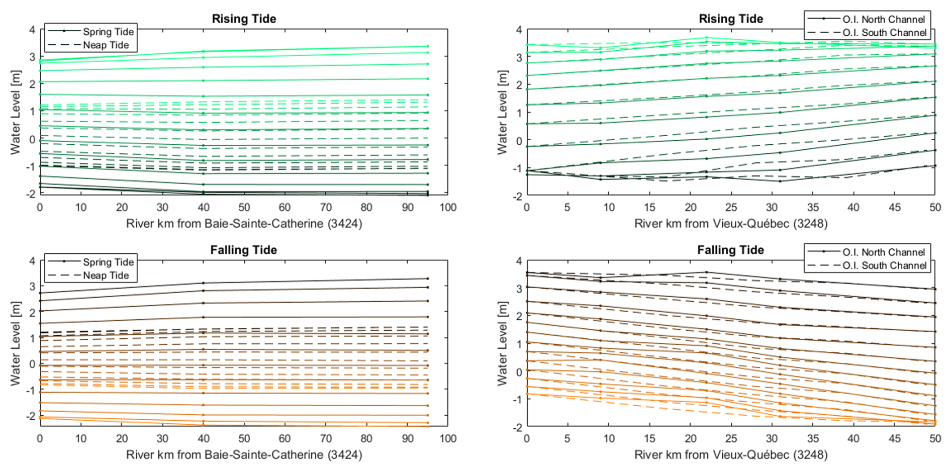
Figure 10Longitudinal water level profiles during rising (first row) and falling tides (second row): (left) Saguenay Fjord water levels during spring and neap tides (6 and 12 July 2023, respectively) at stations 3424, 3440, and 3460; (right) St. Lawrence River water levels around Orleans Island (O.I.) (1 and 2 November 2023) at stations ptio, chri, sab2, and 3075 in the North channel, and stations 3110, sjio, 3100, and 3190 in the South channel. Darker to lighter colors are in chronological order, each line being separated by 30 min.
5.2 Wave data validation
5.2.1 Wave and wind conditions captured by IML-4 during 2023 and 2024
The St. Lawrence deep-water wave system can be synthesized as a wind-driven sea limited to the estuarine stretch. In specific circumstances, swells may form locally or penetrate westward from the estuary's outlet, where it widens into the Gulf. Such wave regimes are likely to evolve on scales larger than, or comparable to, the selected cutoff wavelength of 200 m (corresponding to a period of 11.3 s). Henceforth, the choice of a cutoff criterion intends to mitigate the contamination from slow-frequency motions unrelated to wave motions, although its selection has not been fully tested against all possible wave regimes. The objective is to ensure that the buoy's measurements remain physically meaningful and interpretable for wind seas. Considering this, we delved a bit further using the wave age criterion as defined by Hanson and Phillips (2001), which classifies the filtered wave system as either wind sea or swell, based on whether
where cp is the wave phase velocity, represents the angle between the wind and wave directions, while U10 is the wind speed measured at 10 m, which follows a logarithmic profile, , as described in Hsu et al. (1994). This equation uses the wind speed Uazmp(z) measured at an approximate height of z=4.3 m atop the buoy's mast.
Figure 11 illustrates the relationship between the wind and wave system over the course of the 2023 and 2024 seasons. The wave's direction of propagation adjusts to the wind provenance (panel a), emphasizing that two states of which wind and waves propagate coincidentally along St. Lawrence are more likely observed, that is, approximately 50 and 230° relative to true north. Figure 11b presents a comparison between the wind component U10 parallel to waves and the dominant wave's phase velocity. Partitions that satisfy Eq. (4) are above the gray line cp=1.5U10, and they are highlighted in red in both panels, representing approximately 80 % of all the wind conditions measured in 2023 and 2024. The vast majority of the wave dynamics captured by IML-4 are likely representative of wind-driven wave regimes in the selected frequency range.
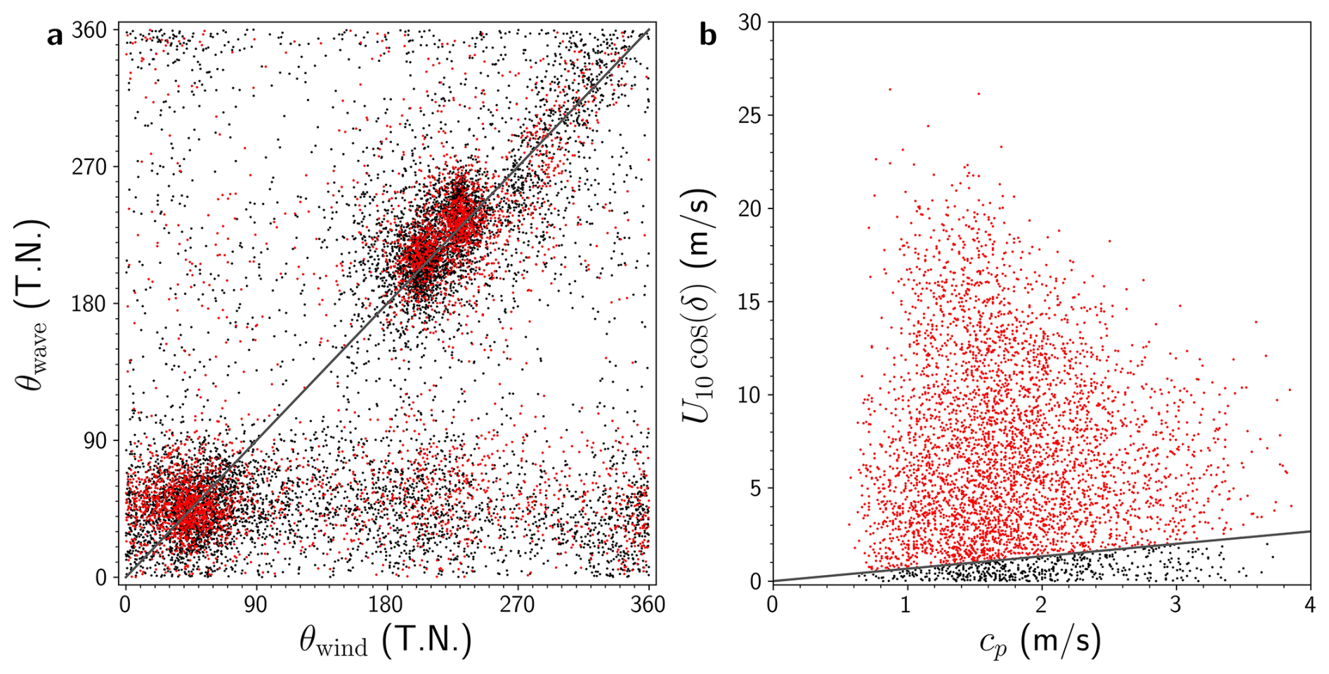
Figure 11Wave origin and age, as observed by IML-4, under the wind conditions experienced in 2023 and 2024: (a) Scatter plot of wind speed versus the average wave provenance; (b) Comparison of wave phase velocity cp and the wind component U10 parallel to the wave direction of propagation.
5.2.2 Comparing IML-4 to Spotter during 2023
We continued our exploration of the St. Lawrence wave system by comparing wave spectra and bulk wave parameters between the IML-4 and Spotter buoy in Les Escousmins (spot-1082). Figure 12a, b illustrate the spectrograms of the variance wave spectra for both buoys. Strikingly, the observations are very similar, despite the buoys being more than 60 km apart. Dominant waves propagate with an average phase velocity of 1.5–2.5 m s−1. The waves are slightly faster and weaker nearshore, as measured by Spotter-1082. Panels (c), (d), (e) present the significant wave height hm0, mean zero-crossing period Tm02, and mean wave provenance measured by each station, with colored stars indicating wave parameters that have been raised for failing quality control, regardless of the test. The significant wave height can reach up to 2 m, but it may increase further in response to strong localized wind events (Fig. 12c). In a similar fashion, the mean zero-crossing period and provenance are provided for SWOT validation (Fig. 12d, e). Differences between the two buoys are summarized in Table 7.
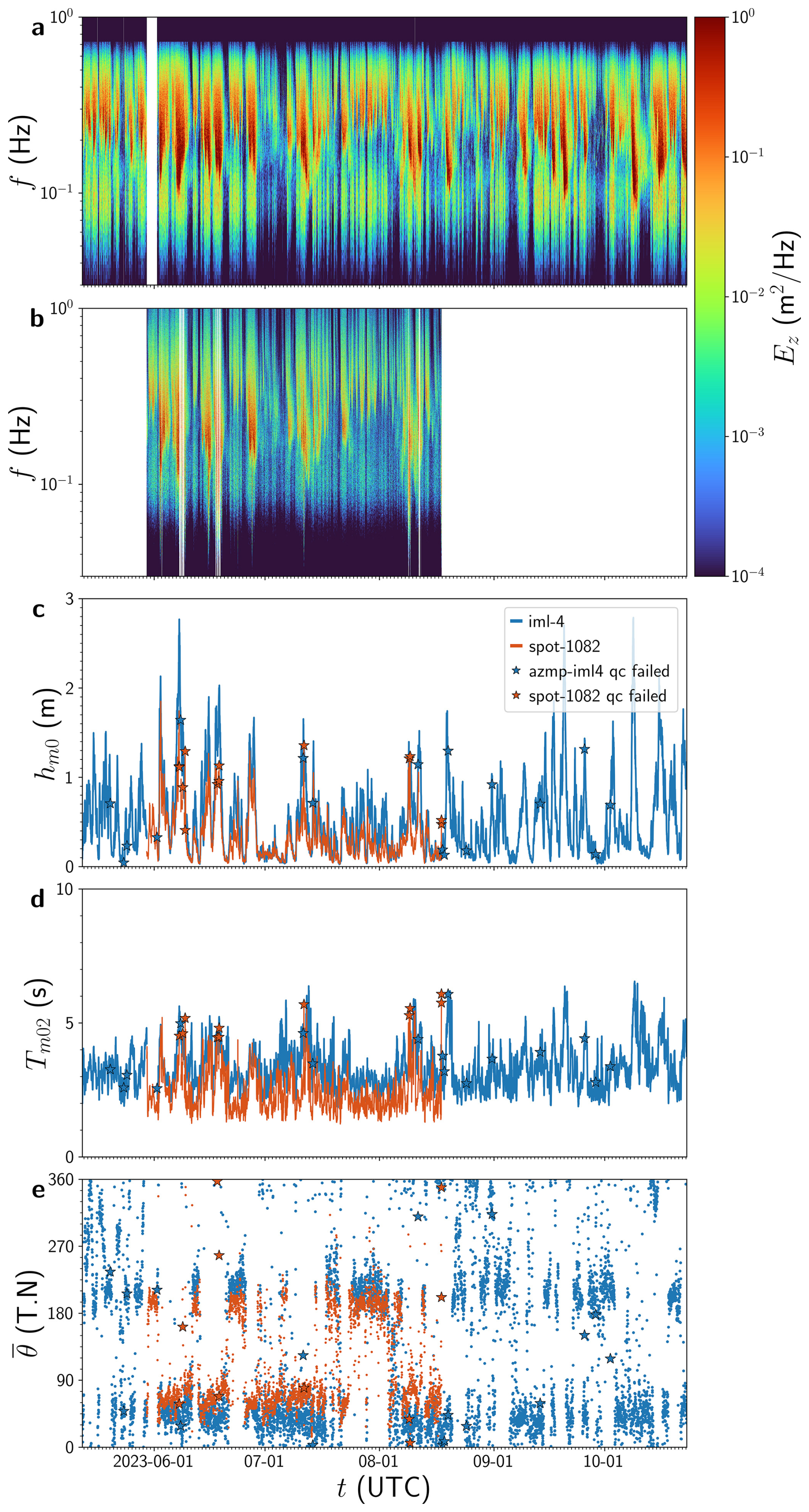
Figure 12Comparing wave conditions between Rimouski (IML-4) and Les Escoumins (Spotter), across the St. Lawrence Lower Estuary, from May to November 2023. Panels (a) and (b) show the spectrograms of IML-4 and Spotter's wave variance spectrum, respectively. Panels (c), (d) and (e) display the significant wave height, mean zero-crossing period, and mean wave provenance for each buoy. Stars indicate data that have been categorized as fail or suspicious by quality control.
Table 7Comparison between Viking (azmp-iml4) and Spotter (spot-1082) wave buoys in the St. Lawrence Estuary. Metrics include root-mean-squared difference (RMSD), mean difference, maximum absolute difference, and the number of matching points used for comparisons between the two sensors. For angular data, circular distances are used.
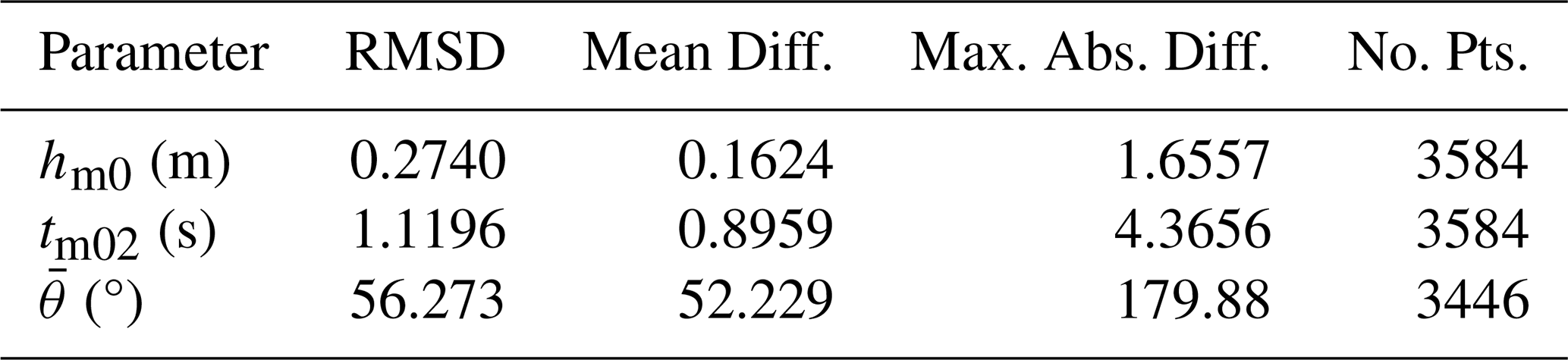
While the two buoys experience similar variability, mean differences are visible and likely linked to their respective location in the estuary (offshore vs. nearshore). Moreover, Spotter and IML-4 platforms differ in several ways. First, the GPS signal's intermittency can cause temporary disruptions in the Spotter data stream. Second, the Spotter hub, weighing around 8 kg and measuring 42 cm × 31 cm, is more sensitive to high-frequency wave motions than the larger IML-4 platform. Third, by measuring the second derivative of surface displacements, IML-4 has a responsiveness to high-frequency waves reduced by a factor of ω−4, where ω is the wave frequency, rendering it insensitive to oscillations above approximately 0.7 Hz. A detailed performance comparison of the two instruments, however, lies beyond the scope of this work.
The presented benchmark dataset of water levels and waves is available at https://doi.org/10.5281/zenodo.18225504 (Matte et al., 2026). Updates are targeted approximately annually, depending on data retrieval, processing, and quality-control activities. The GNSS-IR processing software is available at https://github.com/purnelldj/gnssir_rt (Purnell et al., 2024b). Processing routines for AZMP and Spotter buoys, including quality control, are available at https://github.com/xavier-chartrand/AZMP.git (Chartrand, 2026a) and https://github.com/xavier-chartrand/Spotter.git (Chartrand, 2026a), respectively.
7.1 Summary and perspectives
This paper presents a comprehensive in situ dataset of water level and wave records acquired in the St. Lawrence Estuary and Saguenay Fjord (Quebec, Canada) during the SWOT satellite mission's fast-sampling (Cal/Val) and early science phases (March–July 2023, and ongoing). The dataset represents the densest observational network ever deployed in this region, spanning two of the most hydrodynamically complex areas of the St. Lawrence System: the estuarine transition zone between Orleans Island and Baie-Saint-Paul, and the head of the Laurentian Channel near the Saguenay Fjord.
The measurements were strategically acquired to coincide with SWOT overpasses during its 3-month Cal/Val period, with stations distributed across the satellite’s swath and nadir tracks. This spatial coverage will enable a detailed assessment of SWOT’s performance under contrasting environmental conditions and as a function of orbit geometry and layover conditions (Durand et al., 2020), including both nadir and KaRIn wide-swath altimetry products. As SWOT transitioned to its nominal 21 d repeat orbit in July 2023, the continued in situ data collection allows extended validation of SWOT products in a macro-tidal fluvial-estuarine context. Furthermore, the availability of data in both SWOT’s high-rate (HR) and low-rate (LR) modes broadens its applicability for researchers evaluating these distinct observation products.
A rigorous, standardized quality control and validation framework has been applied to all water level and wave data, ensuring internal consistency and reliability across the diverse sensor network. Comparison of pressure gauge, GNSS-IR, and wave buoy data against reference stations demonstrates high measurement accuracy, with typical root-mean-square differences in the 1–10 cm range for water levels and robust agreement in wave parameters across buoy types. Quality control algorithms effectively detected and flagged anomalies related to environmental, instrumental, or referencing errors, ensuring only high-confidence data are disseminated. These validation efforts provide users with comprehensive metadata and uncertainty estimates, making this dataset well suited for satellite validation and modeling applications.
Beyond SWOT validation, this dataset also supports the calibration and validation of numerical hydrodynamic models and complementary observing systems, including the high-frequency radars deployed during the SWOT Cal/Val period and the AirSWOT campaign conducted in August 2023 (Simard et al., 2023). These independent in situ observations provide valuable reference data for assessing the accuracy and uncertainty of these complementary observing systems, while also opening new avenues for investigating key processes such as tidal wave propagation, wave-current interactions, and the generation of topographic and internal waves and tides. Additionally, the dataset includes pre-processed auxiliary variables that offer further insights – for example, enabling the assessment of surface roughness under wavy or icy conditions – thereby broadening its range of potential applications.
This dataset marks the first spatially dense observational network capable of providing a comprehensive characterization of tidal dynamics in the St. Lawrence Estuary and Saguenay Fjord, with standardized quality control and validation protocols ensuring its value as a benchmark for current and future estuarine research.
7.2 Limitations
Despite its breadth, the dataset suffers from some limitations. Issues with Seametrics CT2X sensor readings and occasional exposure of pressure transducers during low tides were encountered, reducing the length of some records or truncating the low water levels. Additionally, certain stations located in the estuarine transition zone lack salinity data, potentially leading to the underestimation of water levels around high tides.
GNSS-IR data interpolation, while generally very precise compared to pressure gauges, presents challenges, particularly around high and low tides. These challenges could be addressed through improved processing methods. Additionally, seasonal data gaps were observed during winter due to reduced daylight and battery failure caused by cold temperatures.
Finally, the uncorrected Doppler shifts resulting from horizontal buoy movements can have an important impact on wave data. However, fast sampling of these movements, followed by their subsequent processing, is needed to quantify the magnitude of such biases.
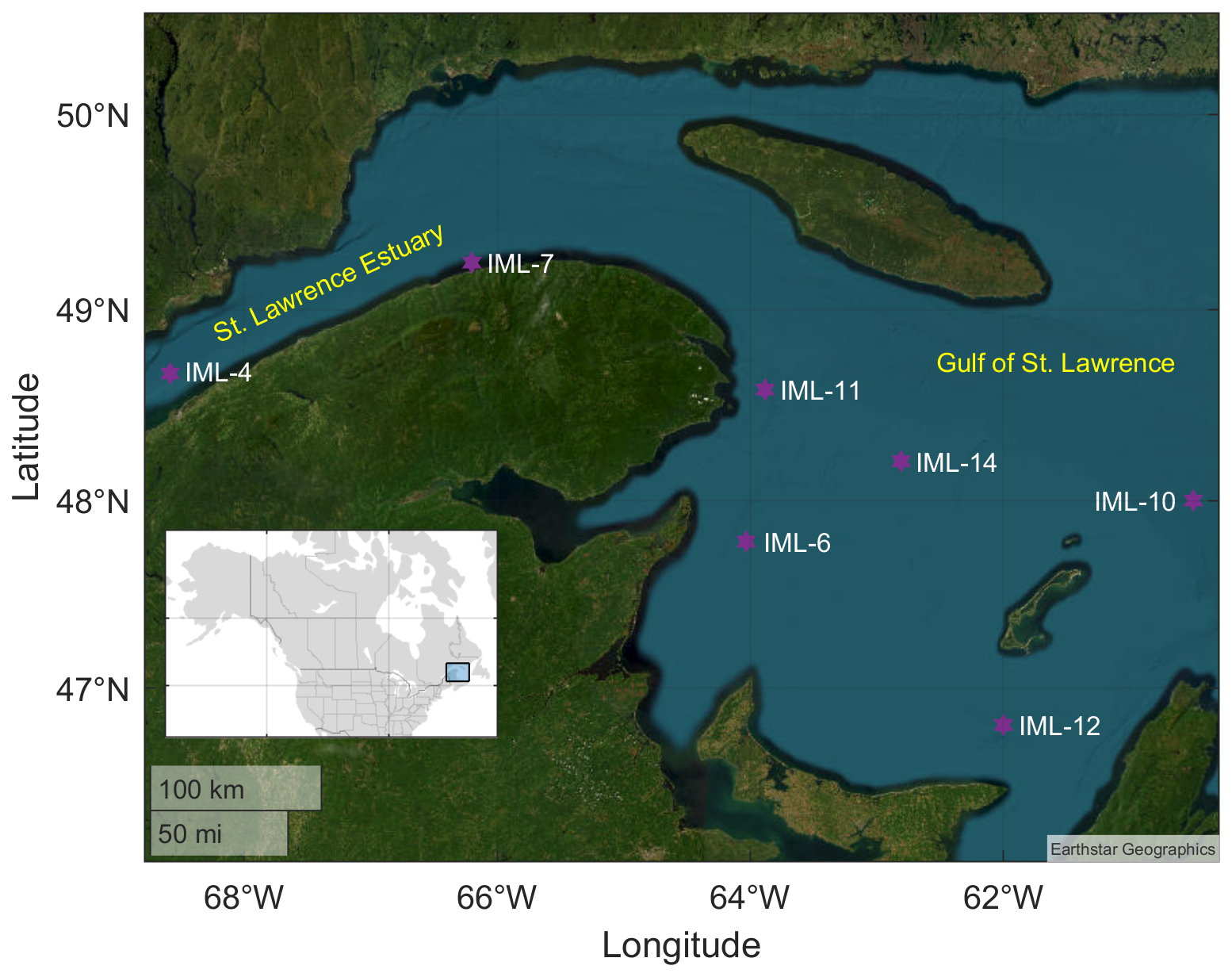
Figure 13Additional Viking wave buoys in the St. Lawrence Estuary and Gulf as part of the AZMP, to be added in a future release of the database.
7.3 Future updates
The current dataset is geographically limited to the SWOT Cal/Val orbit. However, to support future SWOT validation activities, additional tide gauges, GNSS-IR sensors, and wave buoys will be incorporated at new locations along the St. Lawrence River, including in upstream tidal and fluvial reaches and in the downstream Gulf of St. Lawrence, leveraging near-global SWOT coverage during the Science phase. Relying in part on existing stations maintained by DFO, Fig. 13 shows a network of active wave buoys in the Gulf of St. Lawrence that is planned to be incorporated in the next version of the dataset.
Future updates will also be made as new data are retrieved and processed. In addition, new Level 3 (L3) data products could be introduced – for example, derived from GNSS-IR data – including parameters relevant to applications such as ice-on/ice-off period detection, ice characterization, and significant wave height estimation (Purnell et al., 2024a).
This evolving dataset will continue to support hydrodynamic research and SWOT validation, and serve as a long-term benchmark for observing complex estuarine environments.
Table A1Water level stations metadata and conversion factors (see Eq. 3) in the Saguenay Fjord and St. Lawrence Estuary.
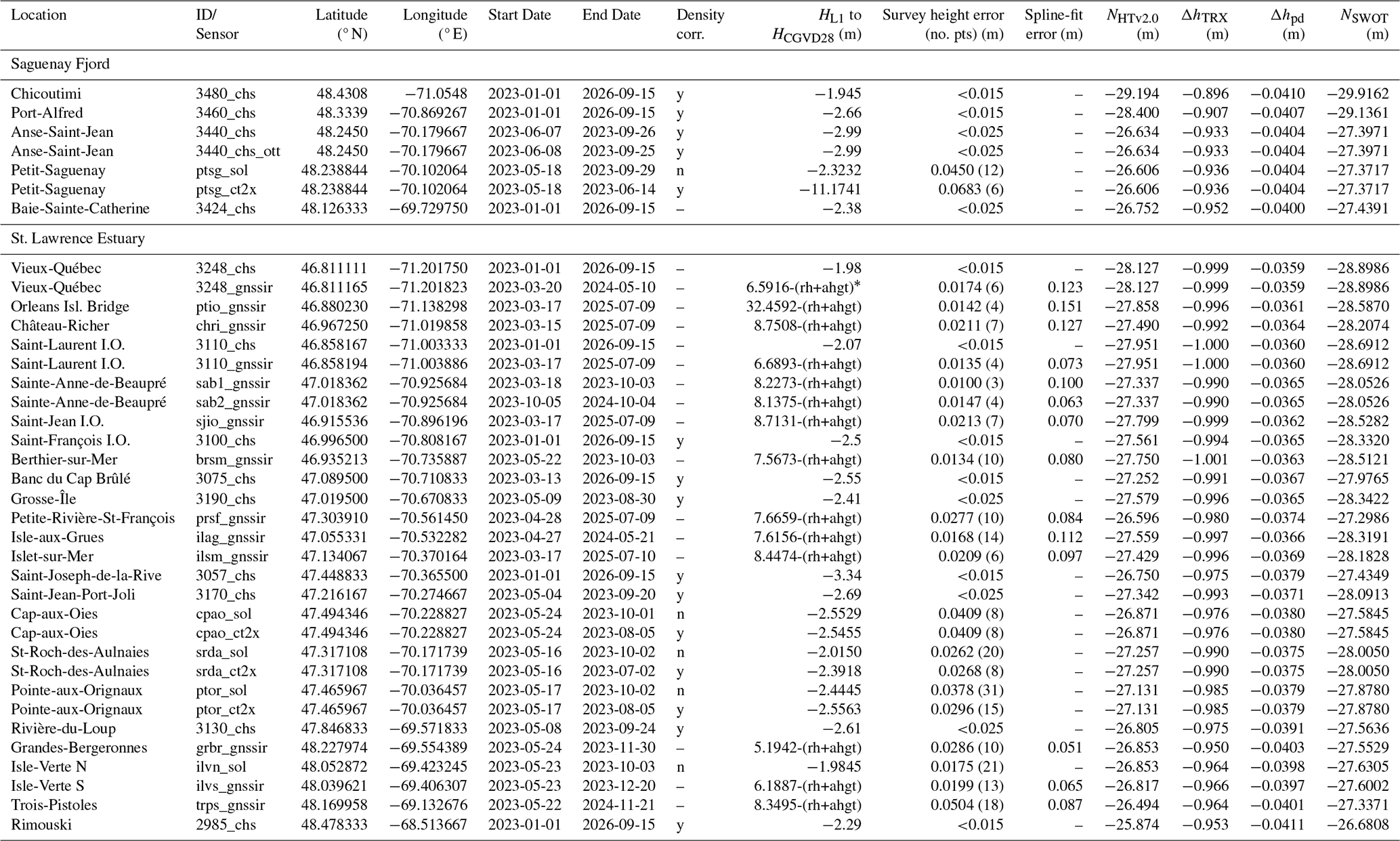
* Definitions of rh and ahgt variables can be found in Table A2.
Table A2Variables included in Level 1 and Level 2 water level files. For a complete description of GNSS-IR variables, refer to Purnell et al. (2024a, b).

Table A3St. Lawrence Estuary wave buoys. The ID given in column 3 is dependent on the buoy type and its assigned number or name. The geoposition corresponds to the water depth, longitude and latitude at the centroid of the buoy's operating area, expressed in decimal degrees, using the WSG84 geodetic datum. Start and end dates correspond to deploying and dismantling dates, respectively.

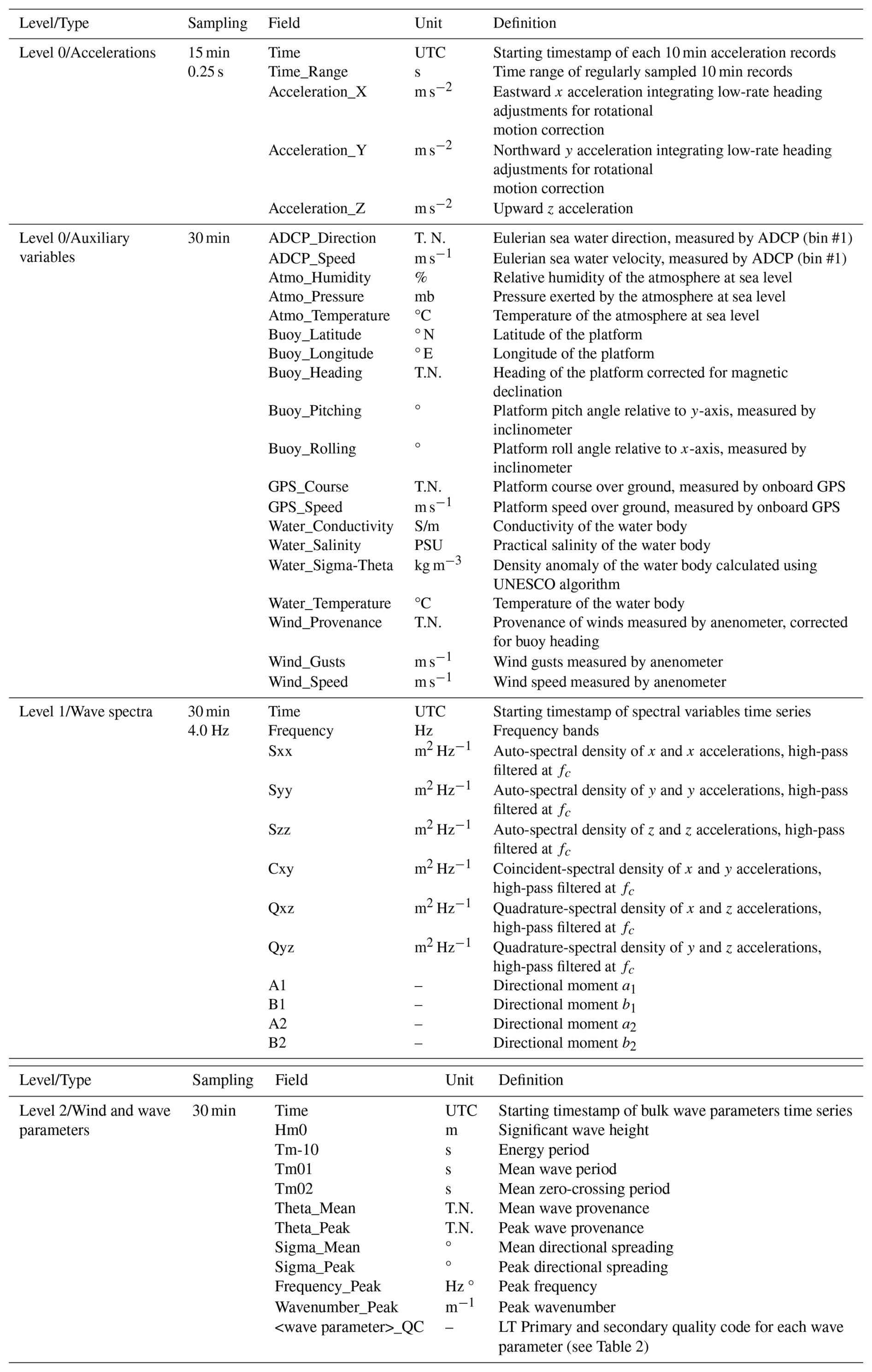
Table A5Variables included in Level 0, 1 and 2 of Spotter wave datasets.
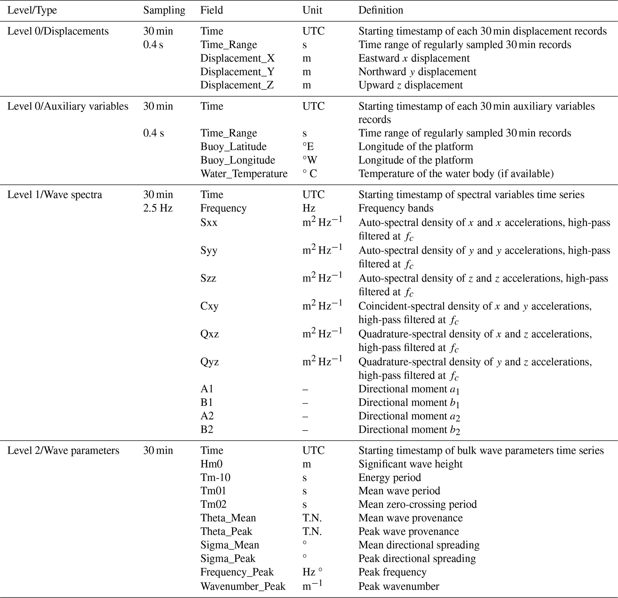
PM: conceptualization, data curation, formal analysis, funding acquisition, investigation, methodology, resources, supervision, validation, writing (original draft preparation). XC: data curation, formal analysis, investigation, software, writing (original draft preparation). DP: data curation, formal analysis, investigation, software, validation, writing (original draft preparation). MS: conceptualization, funding acquisition, resources, writing (review and editing). AC: data curation, validation, writing (review and editing). FFL: supervision, data curation, writing (review and editing). JM: resources, writing (review and editing). YCN: data curation, writing (review and editing). ÉD: data curation, writing (review and editing). AO: data curation, writing (review and editing). CC: funding acquisition, resources, supervision, writing (review and editing). FA: conceptualization, funding acquisition, project administration, resources, supervision. GS: methodology, supervision, writing (review and editing). SB: data curation, writing (review and editing). SI: data curation, writing (review and editing). MD: conceptualization, writing (review and editing). DLP: conceptualization, writing (review and editing). MT: writing (review and editing).
The contact author has declared that none of the authors has any competing interests.
Publisher's note: Copernicus Publications remains neutral with regard to jurisdictional claims made in the text, published maps, institutional affiliations, or any other geographical representation in this paper. The authors bear the ultimate responsibility for providing appropriate place names. Views expressed in the text are those of the authors and do not necessarily reflect the views of the publisher.
Special thanks go to the Canadian Hydrographic Survey for contributing four temporary tide gauge installations. We also warmly thank Jérémy Baudry from UQAR-ISMER for sharing code for the analysis of wave buoy data.
This research has been supported by the Canadian Space Agency (grant nos. 19SUSWEC and 21SUESPVSW), the Nature et technologies (grant no. 2024-PR-326974), and the National Aeronautics and Space Administration, Jet Propulsion Laboratory (grant nos. 80NM0018D0004 and NNH23ZDA001N-SWOTST).
This paper was edited by Alessio Rovere and reviewed by two anonymous referees.
Belzile, M., Galbraith, P. S., and Bourgault, D.: Water renewals in the Saguenay Fjord, J. Geophys. Res.-Oceans, 121, 638–657, 2016. a
Bizhanimanzar, M., Rondeau-Genesse, G., Caron, L. P., Lefaivre, D., and Mailhot, E.: Joint Occurrence of Extreme Water Level and River Flows in St. Lawrence River Coasts Under Present and Sea Level Rise Conditions, Earth's Future, 12, e2023EF004027, https://doi.org/10.1029/2023EF004027, 2024. a
Bourgault, D. and Kelley, D. E.: Wave-induced boundary mixing in a partially mixed estuary, J. Mar. Res., 61, 553–576, 2003. a
Bourgault, D. and Matte, P.: A Physically Based Method for Real-Time Monitoring of Tidal River Discharges From Water Level Observations, With an Application to the St. Lawrence River, J. Geophys. Res.-Oceans, 125, e2019JC015992, https://doi.org/10.1029/2019JC015992, 2020. a
Bourgault, D., Chavanne, C., Dumont, D., Morin, E., Galbraith, P., and Gostiaux, L.: Le point sur les marées d'équinoxes dans l'estuaire du Saint-Laurent, Nat. Can., 140, 73–84, 2016a. a
Bourgault, D., Galbraith, P. S., and Chavanne, C.: Generation of internal solitary waves by frontally forced intrusions in geophysical flows, Nat. Commun., 7, 13606, https://doi.org/10.1038/ncomms13606, 2016b. a
Bushnell, M.: Manual for Real-Time Quality Control of In-Situ Surface Wave Data: A Guide to Quality Control and Quality Assurance of In-Situ Surface Wave Observations Version 2.1., https://doi.org/10.25923/7yc5-vs69, 2019. a
Chartrand, X.: xavier-chartrand/AZMP: ESSD AZMP (Version v1.0), Zenodo [code], https://doi.org/10.5281/zenodo.22961661, 2026a. a
Chartrand, X.: xavier-chartrand/Spotter: ESSD Spotter (Version v1.0), Zenodo [code], https://doi.org/10.5281/zenodo.22961954, 2026b. a
D’Ovidio, F., Pascual, A., Wang, J., Doglioli, A.M., Jing, Z., Moreau, S., Grégori, G., Swart, S., Speich, S., Cyr, F., Legresy, B., Chao, Y., Fu, L., and Morrow, R. A.: Frontiers in Fine-Scale in situ Studies: Opportunities During the SWOT Fast Sampling Phase, Front. Mar. Sci., 6, 168, https://doi.org/10.3389/fmars.2019.00168, 2019. a
Durand, M., Chen, C., de Moraes Frasson, R. P., Pavelsky, T. M., Williams, B., Yang, X., and Fore, A.: How will radar layover impact SWOT measurements of water surface elevation and slope, and estimates of river discharge?, Remote Sens. Environ., 247, 111883, https://doi.org/10.1016/j.rse.2020.111883, 2020. a
Elmi, O., Tourian, M. J., Saemian, P., and Sneeuw, N.: Remote Sensing-Based Extension of GRDC Discharge Time Series-A Monthly Product with Uncertainty Estimates, Sci. Data, 11, 240, https://doi.org/10.1038/s41597-024-03078-6, 2024. a
El-Sabh, M. I., Lie, H.-J., and Koutitonsky, V. G.: Variability of the Near-Surface Residual Current in the Lower St. Lawrence Estuary, J. Geophys. Res.-Oceans, 87, 9589–9600, 1982. a
Forrester, W. D.: Internal tides in St. Lawrence estuary, J. Mar. Res., 32, 55–66, 1974. a
Fu, L.-L., Pavelsky, T., Cretaux, J.-F., Morrow, R., Farrar, J. T., Vaze, P., Sengenes, P., Vinogradova-Shiffer, N., Sylvestre-Baron, A., Picot, N., and Dibarboure, G.: The Surface Water and Ocean Topography Mission: A breakthrough in radar remote sensing of the ocean and land surface water, Geophys. Res. Lett., 51, e2023GL107652, https://doi.org/10.1029/2023GL107652, 2024. a
Godin, G.: The Propagation of Tides up Rivers with Special Considerations on the Upper Saint Lawrence River, Estuar. Coast. Shelf S., 48, 307–324, 1999. a
Haigh, I. D., Marcos, M., Talke, S. A., Woodworth, P. L., Hunter, J. R., Hague, B. S., Arns, A., Bradshaw, E., and Thompson, P.: GESLA version 3: A Major Update to the Global Higher-Frequency Sea-Level Dataset, Geosci. Data J., 10, 293–314, 2023. a
Hanson, J. L. and Phillips, O. M.: Automated analysis of ocean surface directional wave spectra, J. Atmos. Ocean. Tech., 18, 277–293, 2001. a
Hopkinson, C., Crasto, N., Marsh, P., Forbes, D., and Lesack, L.: Investigating the spatial distribution of water levels in the Mackenzie Delta using airborne LiDAR, Hydrol. Process., 25, 2995–3011, 2011. a
Hsu, S. A., Meindl, E. A., and Gilhousen, D. B.: Determining the power-law wind-profile exponent under near-neutral stability conditions at sea, J. Appl. Meteorol., 757–765, https://doi.org/10.1175/1520-0450(1994)033<0757:DTPLWP>2.0.CO;2, 1994. a
JPL D-109532, Revision A: SWOT Science Data Products User Handbook, Jet Propulsion Laboratory Internal Document, Pasadena, CA, https://archive.podaac.earthdata.nasa.gov/podaac-ops-cumulus-docs/web-misc/swot_mission_docs/D-109532_SWOT_UserHandbook_RevA_20250311_sig-final.pdf (last access: 26 September 2026), 2025. a, b, c
Kim, S. K., Lee, E., Park, J., and Shin, S.: Feasibility Analysis of GNSS-Reflectometry for Monitoring Coastal Hazards, Remote Sens., 13, 976, https://doi.org/10.3390/rs13050976, 2021. a
Little, S., Lewis, J. P., and Pietkiewicz, H.: Defining Estuarine Squeeze: The Loss of Upper Estuarine Transitional Zones Against In-Channel Barriers Through Saline Intrusion, Estuar. Coast. Shelf S., 278, 108107, https://doi.org/10.1016/j.ecss.2022.108107, 2022. a
Matte, P., Secretan, Y., and Morin, J.: Hydrodynamic Modeling of the St. Lawrence Fluvial Estuary. I: Model Setup, Calibration, and Validation, J. Waterw. Port C., 143, 04017010, https://doi.org/10.1061/(ASCE)WW.1943-5460.0000397, 2017a. a
Matte, P., Secretan, Y., and Morin, J.: Hydrodynamic Modeling of the St. Lawrence Fluvial Estuary. II: Reproduction of Spatial and Temporal Patterns, J. Waterw. Port C., 143, 04017011, https://doi.org/10.1061/(ASCE)WW.1943-5460.0000394, 2017b. a
Matte, P., Secretan, Y., and Morin, J.: Drivers of residual and tidal flow variability in the St. Lawrence fluvial estuary: Influence on tidal wave propagation, Cont. Shelf Res., 174, 158–173, 2019. a
Matte, P., Chartrand, X., and Purnell, D.: Benchmark dataset of water levels and waves in the St. Lawrence Estuary and Saguenay Fjord, Quebec, Canada (1.0.0), Zenodo [data set], https://doi.org/10.5281/zenodo.18225504, 2026. a, b, c
Meran, G., Siehlow, M., and von Hirschhausen: Integrated Water Resource Management: Principles and Applications, The Economics of Water: Rules and Institutions, 23–121, https://doi.org/10.1007/978-3-030-48485-9_3, 2021. a
Mertz, G. and Gratton, Y.: Topographic Waves and Topographically Induced Motions in the St. Lawrence Estuary BT – Oceanography of a Large-Scale Estuarine System: The St. Lawrence, in: Oceanography of a Large-Scale Estuarine System: The St. Lawrence, edited by: El-Sabh, M. I. and Silverberg, N., Springer New York, 94–108, ISBN 978-1-4615-7534-4, https://doi.org/10.1007/978-1-4615-7534-4_5, 1990. a
Mertz, G., El-Sabh, M. I., Proulx, D., and Condal, A. R.: Instability of a Buoyancy-Driven Coastal Jet: The Gaspé Current and its St. Lawrence Precursor, J. Geophys. Res.-Oceans, 93, 6885–6893, 1988. a
Mishra, A. K. and Coulibaly, P.: Developments in Hydrometric Network Design: A review, Rev. Geophys., 47, https://doi.org/10.1029/2007RG000243, 2009. a
Moftakhari, H. R., Jay, D. A., and Talke, S. A.: Estimating river discharge using multiple-tide gauges distributed along a channel, J. Geophys. Res.-Oceans, 121, 2078–2097, 2016. a
Mulligan, R. P., Swatridge, L., Cantelon, J. A., Kurylyk, B. L., George, E., and Houser, C.: Local and Remote Storm Surge Contributions to Total Water Levels in the Gulf of St. Lawrence During Hurricane Fiona, J. Geophys. Res.-Oceans, 128, e2023JC019910, https://doi.org/10.1029/2023JC019910, 2023. a
Nikolaidou, T., Santos, M. C., Williams, S. D. P., and Geremia-Nievinski, F.: Raytracing atmospheric delays in ground-based GNSS reflectometry, J. Geodesy, 94, 68, https://doi.org/10.1007/s00190-020-01390-8, 2020. a
Nikolaidou, T., Santos, M. C., Williams, S. D. P., and Geremia-Nievinski, F.: Development and Validation of Comprehensive Closed Formulas for Atmospheric Delay and Altimetry Correction in Ground-Based GNSS-R, IEEE T. Geosci. Remote, 61, 1–7, 2023. a
Purnell, D., Gomez, N., Chan, N. H., Strandberg, J., Holland, D. M., and Hobiger, T.: Quantifying the Uncertainty in Ground-Based GNSS-Reflectometry Sea Level Measurements, IEEE J. Sel. Top. Appl., 13, 4419–4428, 2020. a
Purnell, D. J., Gomez, N., Minarik, W., Porter, D., and Langston, G.: Precise water level measurements using low-cost GNSS antenna arrays, Earth Surf. Dynam., 9, 673–685, https://doi.org/10.5194/esurf-9-673-2021, 2021. a
Purnell, D., Dabboor, M., Matte, P., Peters, D., Anctil, F., Ghobrial, T., and Pierre, A.: Observations of River Ice Breakup Using GNSS-IR, SAR and Machine Learning, IEEE T. Geosci. Remote, 62, 1–13, https://doi.org/10.1109/TGRS.2024.3380554, 2024a. a, b, c, d
Purnell, D., Gomez, N., Minarik, W., and Langston, G.: Real-Time Water Levels Using GNSS-IR: A Potential Tool for Flood Monitoring, Geophys. Res. Lett., 51, e2023GL105039, https://doi.org/10.1029/2023GL105039, 2024b. a, b, c, d, e, f
Raghukumar, K., Chang, G., Spada, F., Jones, C., Janssen, T., and Gans, A.: Performance characteristics of “Spotter”, a newly developed real-time wave measurement buoy, J. Atmos. Ocean. Tech., 36, 1127–1141, 2019. a
Ruest, B., Neumeier, U., Dumont, D., and Lambert, A.: Wave climate evaluation in the Gulf of St. Lawrence with a parametric wave model, in: Proceedings of Coastal Dynamics 2013: Coastal Dynamics Research Emphasizing Practical Applications, edited by: Bonneton, P. and Garlan, T., Arcachon, France, 24–28 June 2013, Brest, 1363–1374, 2013. a
Ruiz-Martinez, G.: Seawater density from salinity, temperature and pressure, MATLAB central file exchange, https://www.mathworks.com/matlabcentral/fileexchange/85900-seawater-density-from-salinity-temperature-and-pressure (last access: 26 September 2026), 2023. a
Salameh, E., Desroches, D., Deloffre, J., Fjørtoft, R., Mendoza, E. T., Turki, I., Froideval, L., Levaillant, R., Déchamps, S., Picot, N., Laignel, B., and Frappart, F.: Evaluating SWOT's interferometric capabilities for mapping intertidal topography, Remote Sens. Environ., 314, 114401, https://doi.org/10.1016/j.rse.2024.114401, 2024. a
Sassi, M. G., Hoitink, A. J. F., De Brye, B., Vermeulen, B., and Deleersnijder, E.: Tidal impact on the division of river discharge over distributary channels in the Mahakam Delta, Ocean Dynam., 61, 2211–2228, 2011. a
Simard, M., Chao, R., Christensen, A., Denbina, M., and Matte, P.: AirSWOT flies Cal/Val Campaign over the St. Lawrence Estuary, Airborne Science Newsletter, 4–6, https://airbornescience.nasa.gov/sites/default/files/documents/ASPnewsletter_Fall_2023_0.pdf (last access: 26 September 2026), 2023. a, b
Simons, R. D., Monismith, S. G., Saucier, F. J., Johnson, L. E., and Winkler, G.: Modelling Stratification and Baroclinic Flow in the Estuarine Transition Zone of the St. Lawrence Estuary, Atmos.-Ocean, 48, 132–146, 2010. a
Song, M., He, X., Jia, D., Xiao, R., Asgarimehr, M., Wickert, J., Wang, X., and Zhang, Z.: Sea Surface States Detection in Polar Regions Using Measurements of Ground-Based GNSS Interferometric Reflectometry, IEEE T. Geosci. Remote, 60, 1–14, 2022. a
Virtanen, P., Gommers, R., Oliphant, T. E., Haberland, M., Reddy, T., Cournapeau, D., Burovski, E., Peterson, P., Weckesser, W., Bright, J., van der Walt, S. J., Brett, M., Wilson, J., Millman, K. J., Mayorov, N., Nelson, A. R. J., Jones, E., Kern, R., Larson, E., Carey, C. J., Polat, İ., Feng, Y., Moore, E. W., VanderPlas, J., Laxalde, D., Perktold, J., Cimrman, R., Henriksen, I., Quintero, E. A., Harris, C.R., Archibald, A. M., Ribeiro, A. H., Pedregosa, F., van Mulbregt, P., Vijaykumar, A., Bardelli, A. P., Rothberg, A., Hilboll, A., Kloeckner, A., Scopatz, A., Lee, A., Rokem, A., Woods, C. N., Fulton, C., Masson, C., Häggström, C., Fitzgerald, C., Nicholson, D. A., Hagen, D. R., Pasechnik, D. V., Olivetti, E., Martin, E., Wieser, E., Silva, F., Lenders, F., Wilhelm, F., Young, G., Price, G. A., Ingold, G.-L., Allen, G. E., Lee, G. R., Audren, H., Probst, I., Dietrich, J. P., Silterra, J., Webber, J. T., Slavič, J., Nothman, J., Buchner, J., Kulick, J., Schönberger, J. L., de Miranda Cardoso, J. V., Reimer, J., Harrington, J., Rodríguez, J. L. C., Nunez-Iglesias, J., Kuczynski, J., Tritz, K., Thoma, M., Newville, M., Kümmerer, M., Bolingbroke, M., Tartre, M., Pak, M., Smith, N.J., Nowaczyk, N., Shebanov, N., Pavlyk, O., Brodtkorb, P. A., Lee, P., McGibbon, R. T., Feldbauer, R., Lewis, S., Tygier, S., Sievert, S., Vigna, S., Peterson, S., More, S., Pudlik, T., Oshima, T., Pingel, T. J., Robitaille, T. P., Spura, T., Jones, T. R., Cera, T., Leslie, T., Zito, T., Krauss, T., Upadhyay, U., Halchenko, Y. O., Vázquez-Baeza, Y., and SciPy 1.0 Contributors.: SciPy 1.0: Fundamental Algorithms for Scientific Computing in Python, Nat. Methods, 17, 261–272, 2020. a
Ward, N. D., Megonigal, J. P., Bond-Lamberty, B., Bailey, V. L., Butman, D., Canuel, E. A., Diefenderfer, H., Ganju, N. K., Goñi, M. A., Graham, E. B., Hopkinson, C. S., Khangaonkar, T., Langley, J. A., McDowell, N. G., Myers-Pigg, A. N., Neumann, R. B., Osburn, C. L., Price, R. M., Rowland, J., Sengupta, A., Simard, M., Thornton, P. E., Tzortziou, M., Vargas, R., Weisenhorn, P. B., and Windham-Myers, L.: Representing the function and sensitivity of coastal interfaces in Earth system models, Nat. Commun., 11, 2458, https://doi.org/10.1038/s41467-020-16236-2, 2020. a