AGPC: an Annual 500 m Gridded Population (1990–2020) for China incorporating 3D building volume dynamics

Gridded population datasets with long-term temporal coverage and fine spatial resolution are essential for earth system modelling, urban studies, and disaster risk assessment. However, existing population products often fail to adequately represent population distribution in vertically developed urban environments. This paper presents the AGPC dataset, a temporally consistent gridded population dataset for China at 500 m spatial resolution covering the period 1990–2020. AGPC was generated using a machine-learning-based dasymetric mapping framework, integrating multi-source covariates including three-dimensional (3D) building volume, building function, and other socioeconomic variables. County-level census data were used for model calibration, while annual provincial population totals from official statistical yearbooks were applied as constraints to ensure temporal consistency. The SHapley Additive exPlanations (SHAP) analysis confirms the dominant roles of commercial activity intensity and 3D building volume in shaping fine-scale population distribution and highlights the added value of vertical and functional information beyond conventional two-dimensional (2D) indicators. Population estimates were produced annually and aggregated to multiple administrative scales for validation. Comprehensive evaluations demonstrate the reliability and accuracy of the dataset across spatial and temporal scales. At the county level, AGPC shows strong agreement with census data, with correlation coefficients R greater than 0.89 and relative RMSE values below 1 % on the independent validation sets for the baseline years 2010 and 2020. At finer scales, grid-level population estimates aggregated to the township level exhibit high consistency with independent census data with R greater than 0.90, indicating satisfactory capability in capturing finer-scale spatial heterogeneity in population distribution. Multi-temporal validation at the city level for seven time points between 1990 and 2020 yields correlation coefficients ranging from 0.79 to 0.99, indicating stable temporal performance. Comparisons with existing global and regional population datasets show that AGPC better captures population patterns in high-density and vertically developed urban areas, avoiding the density saturation effects commonly observed in 2D products. The AGPC dataset provides a robust and scalable population data resource for long-term socioeconomic and environmental analyses in China, and it is available at https://doi.org/10.6084/m9.figshare.31338352 (Xu et al., 2026).

1 Introduction

The spatial distribution of population is a fundamental component for understanding human–environment interactions (Leyk et al., 2019; Bondarenko et al., 2025). It has been proven that reliable knowledge of population distribution and its spatiotemporal changes serve as a fundamental variable in a broad range of applications, including exposures to climate risk (Chen et al., 2020; MacManus et al., 2021; Doocy et al., 2007; Simarro et al., 2011), interventions in the natural environments (Feng et al., 2021; Wang et al., 2020), provision of public facilities (Song et al., 2018; Chen et al., 2023), and decision-makings from local interventions to global initiatives (McDonald et al., 2011; Doxsey-Whitfield et al., 2015; Tatem, 2014). The demand for timely and spatially detailed population data is particularly strong in regions experiencing rapid urbanization and internal migration, such as East Asia and Latin America (Chen et al., 2024; Cheng et al., 2022; Sorichetta et al., 2015; Tu et al., 2022). In China, in particular, sustainable urban development and evidence-based policymaking rely heavily on accurate and up-to-date gridded population information (Cheng et al., 2022; Tu et al., 2022).

Traditionally, population information has been derived from censuses and civil registration systems that are reported for irregular administrative units and updated at relatively long intervals, typically every 10 years (United Nations, 1980). Such data exhibit substantial heterogeneity in spatial resolution, temporal frequency, and accessibility across countries. Therefore, substantial processing and harmonization are typically required before such data can be used in many analytical workflows (Schroeder, 2007). More importantly, census counts aggregated to administrative units fail to represent the highly uneven spatial distribution of population within those units, especially in densely settled urban areas (Sorichetta et al., 2015). This limitation restricts their direct use in fine-scale spatial analyses and may obscure important subregional disparities.

In recent years, advances in the availability of routinely updated remote sensing observations, increasing computational capacity, and improved statistical and machine-learning techniques have created new opportunities for producing spatially refined population estimates (Chen et al., 2019; Leyk et al., 2019). These approaches, commonly referred to as population downscaling or spatialization, aim to overcome the spatial limitations of census data by redistributing population counts from irregular administrative units to regular grids. The earliest and simplest downscaling approach is areal weighting, also known as proportional reallocation, which redistributes census population evenly to target grid cells based solely on their areal overlap (Goodchild and Lam, 1980; CIESIN, 2018). While computationally efficient, areal weighting implicitly assumes a uniform population distribution within administrative units and therefore fails to capture intra-unit spatial heterogeneity (Salvatore et al., 2005).

To address this limitation, ancillary gridded variables with finer spatial detail, such as nighttime light intensity, impervious surface fraction, and accessibility indicators, have been introduced to inform relative population density. These variables are incorporated through dasymetric mapping methods, which allocate population according to spatially varying weights derived from ancillary data (Zandbergen and Ignizio, 2010; Mennis, 2009; Balk et al., 2006; Salvatore et al., 2005). Correspondingly, a number of global and regional gridded population datasets have been developed using different modelling strategies and ancillary inputs (Leyk et al., 2019). The Gridded Population of the World (GPW) applies areal weighting to generate population grids at 1 km resolution for multiple benchmark years (CIESIN, 2018). The Global Human Settlement Population Grid (GHS-POP) refines population distribution by proportionally allocating census counts according to built-up area fractions at resolutions up to 100 m (Halkia and Carneiro Freire, 2014; Freire et al., 2020). The WorldPop programme further incorporates a wide range of ancillary variables and machine-learning techniques to produce annual global population estimates at resolutions of 100 m to 1 km (Tatem, 2017; Bondarenko et al., 2025). In contrast to these residential population products, LandScan provides annual ambient population estimates at 1 km resolution, representing average population presence over day and night (Dobson et al., 2000).

At the national scale, substantial efforts have also been devoted to developing gridded population datasets for China. For example, Zhao et al. (2020) employed multiple machine-learning methods to disaggregate the county-level census population in 2015 into a 1 km gridded estimate. Similarly, the POP2018 gridded population product was developed by Chen et al. (2022) using log-linear spatially weighted regression to provide ambient population distribution for mainland China at a 0.01° spatial resolution. More recently, Chen et al. (2024) developed a population downscaling approach that leverages stacking ensemble learning models to generate a gridded population dataset for China from the county- and township-level census data in 2020 at a 100 m spatial resolution. Some other high-temporal-resolution population maps were also developed by incorporating mobile phone positioning and other digital footprint data (Cheng et al., 2022; Tu et al., 2022). In addition, several studies have used existing gridded population datasets to project future population distributions under different development scenarios (Chen et al., 2020).

Although substantial progress has been achieved in fine-scale gridded population mapping, several critical limitations remain and deserve further investigation. First, most existing dasymetric population models primarily rely on ancillary variables that characterize horizontal land-surface features, such as built-up area density, nighttime light intensity, POI density, and accessibility to transportation or public facilities (Leyk et al., 2019). While these two-dimensional (2D) indicators are effective in capturing horizontal spatial variation, they cannot fully represent the vertical population-carrying capacity of densely built urban environments. This limitation is particularly pronounced in rapidly urbanizing Chinese cities, where densely developed areas exhibit considerable variation in vertical urban form. Consequently, 2D indicators may obscure substantial differences in population concentration among areas with similar horizontal built-up intensity but contrasting building heights and volumes. Recent studies have begun to address this limitation by incorporating three-dimensional (3D) building information into population mapping. At the national scale, Chen et al. (2024) and Lei et al. (2024) incorporated building height and building volume, respectively, together with other geospatial covariates to produce 100 m gridded population estimates for mainland China. At the urban scale, Yan et al. (2025) and Tu et al. (2026) introduced building height information for fine-scale population estimation in selected Chinese cities, with Tu et al. (2026) further distinguishing residential and non-residential buildings. These studies demonstrate the potential of 3D building information to improve population mapping beyond conventional 2D indicators. Nevertheless, the incorporation of 3D building information into gridded population mapping is still at a relatively early stage, with only a limited number of studies conducted at large spatial scales. Moreover, publicly available and systematically validated gridded population datasets explicitly incorporating 3D building information remain scarce, limiting their broader application and evaluation.

Second, capturing the temporal evolution of the built environment remains another major challenge in long-term population mapping because of its fundamental role in representing population-carrying capacity. Even for gridded population products primarily based on 2D indicators, the built-environment data underlying their spatial allocation are often not routinely or consistently updated. For example, GHS-POP provides annual population estimates, whereas the 2D GHSL built-up layers used for population disaggregation are available only for several benchmark years (1975, 1990, 2000, and 2014) (Freire et al., 2020; Pesaresi et al., 2016). Similarly, the constrained WorldPop product incorporating building footprints is currently available for only a single reference year (Tatem, 2017). This temporal limitation is even more pronounced for 3D building information, as the few existing 3D-based population mapping studies have generally relied on static 3D building data for individual reference years. Consequently, long-term population mapping remains limited in its ability to account for evolving urban structures, including horizontal expansion, increasing building density, and vertical intensification. Temporally consistent 3D built-environment data are therefore essential for capturing these structural changes and their implications for population distribution over time.

Third, building functions remain insufficiently represented in existing population mapping, despite their important role in differentiating population-carrying capacity across urban functions. Most existing population mapping approaches rely on POI data as proxies for urban functions and human activity (e.g., Chen et al., 2024). However, POI datasets tend to provide more complete representations of commercial and public facilities than residential population carriers, because POIs primarily capture identifiable activity and service locations, whereas ordinary residential buildings are less systematically recorded. This imbalance may result in an underrepresentation of residential areas and introduce biases into fine-scale population allocation. Although recent studies have begun to distinguish residential and non-residential buildings (e.g., Tu et al., 2026), the explicit integration of spatially detailed building functions with 3D building structure remains limited, particularly for nationwide population mapping. Explicitly incorporating building functional types can therefore provide complementary information beyond POI-based indicators and better account for the heterogeneous effects of different urban functions on population allocation.

To address these research and data gaps, this study advances conventional dasymetric population modelling by explicitly incorporating multi-temporal 3D urban building characteristics, including building height, volume, and coverage ratio, to characterize changes in population-carrying capacity associated with both horizontal urban expansion and vertical development. In addition, building functional types within settlement areas are explicitly integrated into the construction of dasymetric weights, enabling the model to better differentiate population allocation across urban functions. Together, these enhancements are designed to improve population estimation, particularly in high-rise and densely built urban environments. Based on this enhanced framework, we develop an annual gridded population dataset for China (AGPC) at a 500 m spatial resolution covering the period 1990–2020, supported by a recently developed spatiotemporally consistent 3D urban structure dataset (Liu et al., 2025; Wu et al., 2026). Machine learning models are employed to estimate population distribution weights at 5-year time points from 1990 to 2020 based on 3D building characteristics, building functional types, and other geographic and socioeconomic covariates. These weights are subsequently interpolated to generate a temporally continuous annual sequence, and year-specific official population statistics are then applied as administrative constraints to convert the annual weights into gridded population estimates. Grounded in multi-temporal 3D building information and constrained by official population statistics, AGPC provide a temporally consistent representation of population redistribution associated with the evolving urban built environment. The resulting dataset can support long-term analyses of population dynamics under rapid urbanization and applications such as disaster exposure assessment and urban planning.

2 Data and preprocessing

The data used to derive the AGPC dataset consist of four main components. County-level population census data are used as the dependent variable for dasymetric population modelling. Urban environmental indicators, including routinely updated 3D building characteristics that represent population-carrying capacity, are incorporated as covariates in the modelling framework. Annual provincial-level population totals from official statistical yearbooks spanning 1990–2020 are applied as constraints to ensure consistency between gridded population estimates and census-based demographic records for each year. In addition, township- and city-level population statistics, together with widely used gridded population datasets, are collected for independent validation and comparative evaluation of the resulting population estimates.

2.1 Census and statistical data for population

County-level population census data for mainland China in 2010 (Fig. 1a) and 2020 (Fig. 1b) were obtained from the Sixth and Seventh National Population Censuses of China (Population Census Office under the State Council and National Bureau of Statistics, 2012b; Office of the Leading Group of the State Council for the Seventh National Population Census, 2022a). Here, county-level administrative units refer collectively to counties, urban districts, county-level cities, and other administrative divisions at the equivalent level in China. Population statistics for 2845 such county-level units across mainland China were digitized and linked to corresponding county boundary data acquired from the Tianditu platform (http://www.tianditu.gov.cn, last access: 9 September 2026) (Fig. 1a and b). Hong Kong, Macao, and Taiwan were excluded due to differences in census systems and data availability. For model development and evaluation, the county-level census data were randomly divided into a 70 % training subset and a 30 % independent validation subset. The training subset was used for model fitting and hyperparameter optimization, while the validation subset was held out from the entire training and tuning process and used exclusively for the final evaluation of model performance.

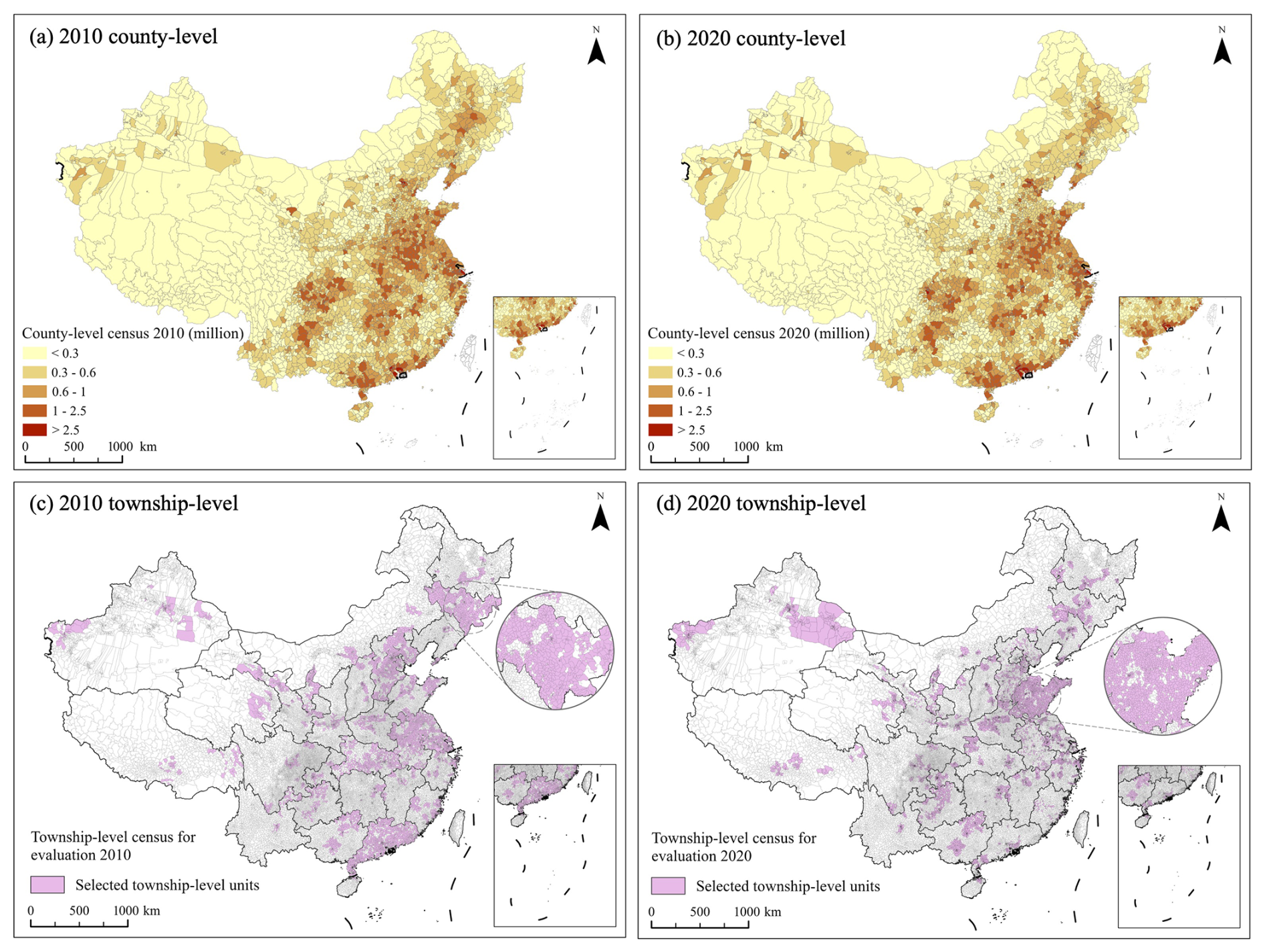
Figure 1 Population census data from Sixth and Seventh National Population Census of China, including county-level population data for 2010 (a) and 2020 (b), and the spatial distribution of selected township-level census units for 2010 (c) and 2020 (d).

Because fine-resolution ground-truth population data are rarely available for direct validation (Leyk et al., 2019), township-level (including towns, townships, and subdistricts) population statistics were collected from the 2010 and 2020 China Population Census tabulations by township (Population Census Office under the State Council and National Bureau of Statistics, 2012a; Office of the Leading Group of the State Council for the Seventh National Population Census, 2022b) for independent assessment. Approximately 10 000 township-level census records were compiled for each of 2010 (Fig. 1c, 10 834 records) and 2020 (Fig. 1d, 10 336 records). As the original township-level census records were primarily available in tabular form without explicit spatial information, they were spatially matched to township administrative boundaries based on administrative names, with ambiguous records manually verified to account for duplicated names, administrative name changes, and boundary adjustments. The resulting validation datasets provide broad geographical coverage across mainland China, with all provinces represented. These township-level records, representing a finer spatial scale than the county-level training data, were used to independently evaluate the accuracy of the gridded population estimates, with a particular focus on the model's ability to capture intra-county spatial heterogeneity. In addition, annual provincial-level population totals for the period 1990–2020 were obtained from official national statistical yearbooks (https://www.stats.gov.cn/english/, last access: 9 September 2026) and applied as constraints to ensure consistency between gridded population estimates and reported demographic statistics for each year. Furthermore, a total of 1501 city-level population records collected from provincial statistical yearbooks for various years were used to validate the temporal consistency and long-term performance of the gridded population time series.

Population data at multiple spatial scales jointly constitute a hierarchical consistency-control framework for gridded population allocation, with each administrative level playing a distinct role in model training, constraint enforcement, and validation. Figure 2 illustrates the hierarchical structure and functional roles of population statistics at different administrative levels within the proposed dasymetric modelling framework. For the baseline years (2010 and 2020), county-level census data are used both as the dependent variable for model training and as total-population constraints for grid-level allocation, while township-level population statistics provide an independent dataset for validating the baseline gridded estimates at a finer spatial scale. For multi-temporal population estimation, provincial-level population statistics are applied as annual total-population constraints to ensure interannual consistency of the gridded time series, and city-level population data are used to evaluate the accuracy and temporal stability of the resulting multi-year gridded population estimates.

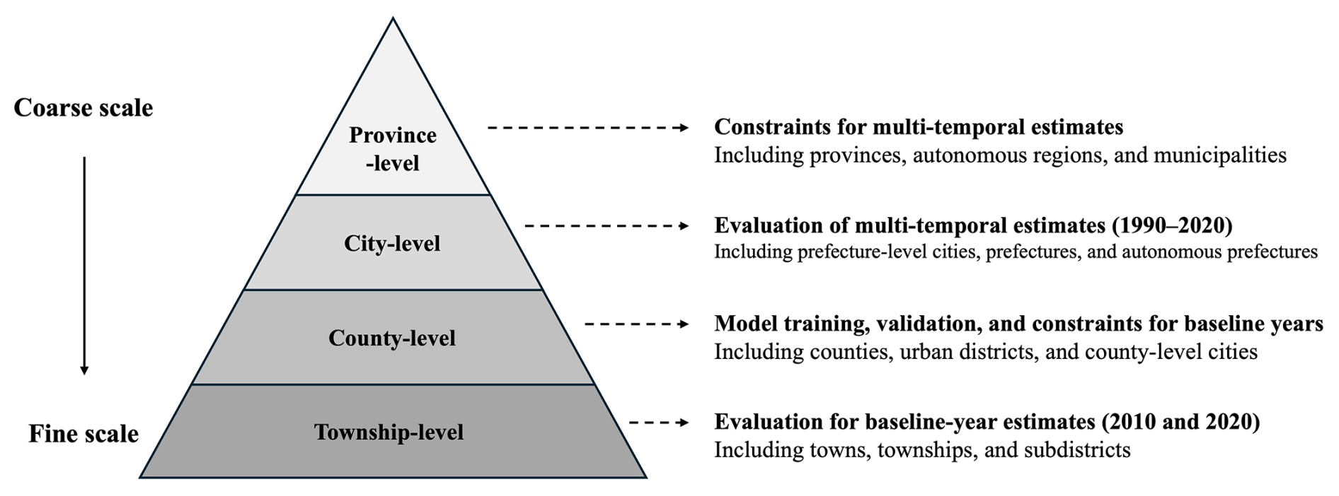
Figure 2 Hierarchy of population census data and their roles in model development, population constraints, and evaluation.

2.2 Urban environmental indicators

Previous studies have consistently demonstrated that population distribution is strongly associated with both natural and socioeconomic factors (Cheng et al., 2022; Leyk et al., 2019; Tu et al., 2022). Building on this foundation, this study further incorporates 3D urban building information to better characterize the built environment and the vertical heterogeneity of population aggregation. Moreover, population distribution is known to exhibit spatial autocorrelation, whereby environmental conditions in neighbouring grid cells may influence local population patterns (Chen et al., 2020). In addition, building functional types within settlement areas are explicitly integrated into the modelling framework, enabling the model to better capture the heterogeneous influences of different urban functions on population spatial distribution. Accordingly, five categories of urban environmental variables, comprising a total of 21 indicators, were selected as model inputs for dasymetric population mapping (Table 1). Together, these variables represent urban 3D structure, building function, socioeconomic activity intensity, transportation accessibility, and natural terrain conditions, providing a multidimensional basis for population disaggregation.

Table 1 Environmental indicators and datasets used in this study.

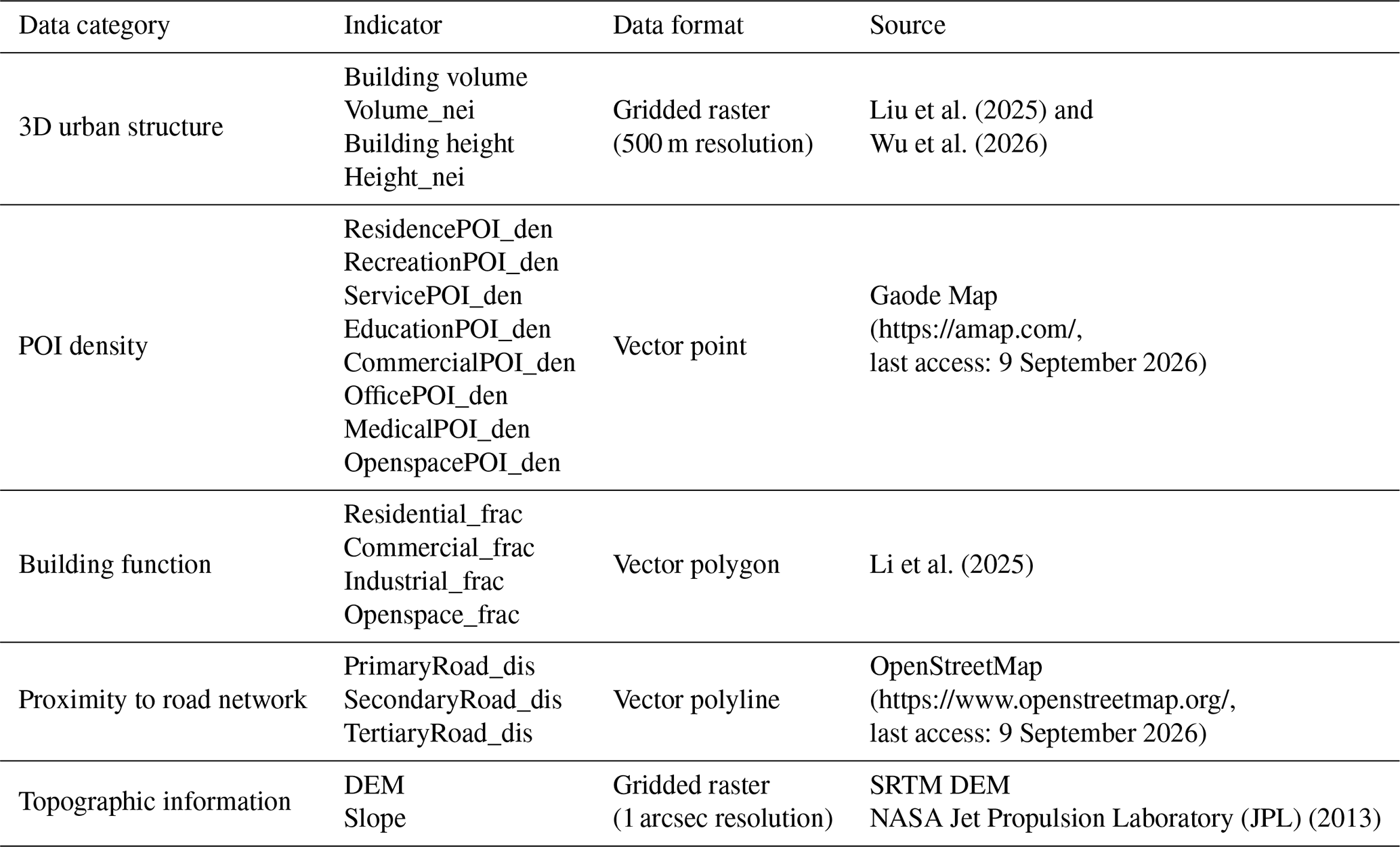
Note: the suffixes _nei, _frac, _den, and _dis denote neighbourhood-effect, fraction-based, density-based, and distance-based indicators, respectively.

2.2.1 3D urban structure dataset

Building-related variables constitute a core component of the gridded population modelling framework. Unlike conventional approaches that rely primarily on 2D land-use indicators or nighttime light data, this study explicitly incorporates 3D urban structure information to quantify the population-carrying capacity of vertical urban space. The 3D building variables were derived from the spatiotemporal GUS-3D dataset developed by our research team (Liu et al., 2025; Wu et al., 2026), which provides global coverage at a 500 m spatial resolution and includes building volume, building footprint ratio, and footprint-area–weighted mean building height for each grid cell. The dataset spans 1990–2020 at 5-year intervals, enabling dynamic characterization of the spatiotemporal evolution of urban 3D structure. The manuscript describing the complete GUS-3D dataset is currently under review (Wu et al., 2026); however, the data used in this study are currently accessible through a private Figshare link provided in the Data Availability section. A permanent public repository and corresponding DOI citation will be provided upon formal publication of the GUS-3D dataset. In this study, building volume and building height were selected as key indicators of population-carrying capacity. To account for neighbourhood effects, mean building volume and mean building height within a 5 × 5 grid-cell window were also included as additional model inputs.

2.2.2 Points of interest data

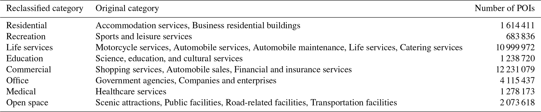
POIs serve as spatial proxies for urban functional facilities and socioeconomic activities and can partially reflect the intensity and type of human activities within cities. POI data were collected from Gaode Map (https://amap.com) through its API in 2020, comprising more than 34 million records. To better capture major urban activity patterns, the original 23 POI categories defined by Gaode Map were aggregated into eight functional types: residential, recreation, life services, education, commercial, office, medical, and open space. Details of the reclassification and record counts are provided in Table 2. Kernel density estimation (KDE) was applied to each POI category to generate density surfaces at a 500 m spatial resolution. A quartic kernel function (Silverman, 2018) with a uniform bandwidth of 2000 m was used for all KDE calculations. Because comparable historical POI archives extending back to the 1990s and early 2000s are generally unavailable, the 2020 POI density surfaces were treated as temporally invariant covariates in the historical reconstruction. It should also be noted that the acquisition year of a POI record does not necessarily correspond to the establishment year of the associated facility.

Table 2 Classification scheme and summary of points of interest used in this study.

2.2.3 Building function dataset

As discussed above, although POI intensity can partially reflect the intensity and types of human activities, residential POIs are typically underrepresented in current map service datasets compared with commercial and public facilities. This imbalance arises from the data production mechanisms of commercial mapping platforms, which tend to prioritize economically active and publicly accessible locations. As a result, large residential compounds are often represented by only a limited number of residential POIs and are frequently surrounded by dense clusters of commercial POIs, leading to a dilution of residential signals. Consequently, it is necessary to explicitly incorporate building functional information into the modelling framework to mitigate the systematic biases introduced by the imbalance in POI representation. Building functional type information in this study was derived from the enhanced essential urban land use categories (EULUC–China 2.0) dataset (Li et al., 2025), which provides detailed level-I urban land-use classifications (residential, commercial, industrial, public, and transportation) in vector format. The dataset was rasterized to a 500 m spatial resolution to ensure consistency with other covariates, with each grid representing the proportional composition of functional types. The rasterized functional layers were further reviewed and corrected through visual interpretation of high-resolution satellite imagery to reduce misclassification and improve the reliability of residential function representation.

2.2.4 Road network information

Road networks are a core component of urban transportation infrastructure and are closely associated with human mobility and daily activities, thereby exerting a strong influence on population agglomeration and spatial distribution. Road network data for China were obtained from OpenStreetMap (https://www.openstreetmap.org/). To represent major transportation structures and routine commuting patterns, only primary, secondary, and tertiary roads were retained. Road accessibility was quantified using Euclidean distance, calculated separately as the distance from the centre of each 500 m grid cell to the nearest road of each class, enabling the model to capture the differentiated effects of road hierarchy on population distribution.

2.2.5 Topographic information

Topographic conditions play an important role in shaping settlement patterns and population distribution. Digital elevation models (DEMs) are therefore widely used in gridded population studies (Ye et al., 2019; Tatem, 2017). Among topographic variables, slope reflects surface suitability for urban development, as flatter terrain generally supports higher population concentrations. DEM data were obtained from the Shuttle Radar Topography Mission (SRTM), jointly released by the National Aeronautics and Space Administration (NASA) and the National Imagery and Mapping Agency (NIMA), at a spatial resolution of 1 arcsec (NASA Jet Propulsion Laboratory (JPL), 2013), and accessed via Google Earth Engine. Slope was derived from the DEM and resampled to a 500 m resolution using the nearest-neighbour method to ensure consistency with other model inputs.

3 Methodology

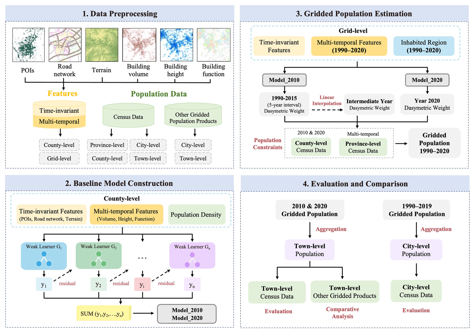
This study aims to generate an annual gridded population dataset (AGPC) for mainland China by explicitly accounting for the population-carrying capacity of 3D building space, building functions, and their temporal evolution. The methodological framework consists of two main stages. First, dasymetric population mapping models were trained and validated for the baseline years 2010 and 2020, when detailed census data and comprehensive urban environmental covariates are available. Multiple machine learning algorithms were employed to learn the relationships between population counts and explanatory variables at the county level. Second, the trained baseline models were extended to the period 1990–2020 at 5-year intervals by incorporating time-varying urban environmental indicators. The resulting dasymetric weights were further interpolated to an annual scale within each 5-year interval to capture continuous temporal dynamics. Annual gridded population estimates were then allocated and constrained using official provincial-level population totals to ensure consistency with reported demographic statistics. The complete workflow is illustrated in Fig. 3, and the detailed modelling procedures are described in the following subsections.

Figure 3 The overall workflow of deriving the AGPC dataset.

3.1 Determine the inhabited region

In this study, census population counts were disaggregated only into inhabited regions to avoid allocating population to uninhabited land covers, following an approach similar to the constrained WorldPop framework (Tatem, 2017). Inhabited regions were primarily identified based on building presence, supplemented with impervious surface data to capture small and fragmented built-up areas. To capture the spatiotemporal dynamics of inhabited regions over the study period (1990–2020), building footprint ratio data from the GUS-3D dataset (Liu et al., 2025; Wu et al., 2026) were integrated with annual impervious surface information extracted from the 30 m Annual Global Land Cover (AGLC) dataset (Li et al., 2026b). The AGLC dataset extends the temporal coverage of impervious surface information originally provided by the Global Annual Urban Dynamics (GAUD) dataset (Liu et al., 2020) to 2022, enabling year-specific impervious surface layers to be used throughout the study period. Because small and fragmented impervious features were partially filtered during the construction of GUS-3D, impervious surface fractions were recalculated at the 500 m grid level from the corresponding annual 30 m AGLC layers and merged with the GUS-3D building footprint ratios to construct a more complete inhabited-region mask for each year. In addition, fragmented settlements not captured by the AGLC dataset, such as small rural villages in mountainous areas (e.g., parts of Sichuan Province), were manually delineated using high-resolution satellite imagery from Google Maps. Building height and volume for these supplementary settlements were assigned based on visual interpretation and surrounding settlement patterns. This procedure further improves the spatial completeness and continuity of inhabited regions, particularly in sparsely populated and topographically complex areas.

3.2 Preparation for county-level covariates and population density

Following established practices in gridded population modelling (Leyk et al., 2019), this study first models the relationship between population density and multidimensional geographic covariates at the county level, and subsequently transfers the learned relationship to the 500 m grid scale for population spatialization. Accordingly, both population statistics and environmental variables were aggregated to the county level for model development. Population density, rather than total population counts, was adopted as the dependent variable, as it is more appropriate for cross-scale comparison and spatial modelling (Ye et al., 2019; Cheng et al., 2022). County-level population density was calculated by dividing the census population count of each county by the area of its inhabited region. A total of 21 indicators (Table 1) were used as environmental covariates in the dasymetric population model.

To ensure comparability among covariates with different units, magnitudes, and distributions, a two-step transformation and normalization procedure was applied before model training. First, all 500 m resolution environmental layers were aggregated to the county level by computing their mean values within each county. Given the pronounced long-tailed distributions observed in most covariates, each county-level covariate was first log-transformed:

$$\begin{array}{}\text{(1)}& x_{ij}^{\prime }=\ln \left(x_{ij}+\mathrm{1}\right)\end{array}$$

where x_ij denotes the original value of covariate j in county i, and $x_{ij}^{\prime }$ is the corresponding log-transformed value. Subsequently, the log-transformed covariates were normalized by their respective national 95th percentiles:

$$\begin{array}{}\text{(2)}& {\stackrel{\mathrm{̃}}{x}}_{ij}={\displaystyle \frac{x_{ij}^{\prime }}{Q_{\mathrm{0.95}}\left(x_j^{\prime }\right)}}\end{array}$$

where ${\stackrel{\mathrm{̃}}{x}}_{ij}$ represents the normalized value used as model input, and Q_0.95(⋅) denotes the 95th percentile of the log-transformed covariate j across all counties nationwide. The resulting normalized county-level covariates were used as explanatory predictors in the machine-learning models. For the response variable, county-level population density was log-transformed to reduce its skewness. To ensure consistency between model training and application, the same transformation and normalization parameters derived at the county-level covariates were subsequently applied to the grid-level covariates during population estimation. This procedure ensures consistent scaling of the explanatory variables between model training and grid-level prediction.

3.3 Weight calculation by machine learning methods

To model the relationship between population density and environmental covariates, we evaluated three machine learning regression approaches: eXtreme Gradient Boosting (XGBoost) (Chen and Guestrin, 2016), a support vector regression (SVR) (Vapnik, 1997), and a random forest (Breiman, 2001). After extensive testing, XGBoost consistently demonstrated the best overall predictive performance during both the training and validation phases (see Table S1 in the Supplement) and was therefore selected as the final modelling approach.

XGBoost is an ensemble method based on gradient boosting decision trees (GBDT), capable of capturing nonlinear relationships and robust against overfitting. Unlike traditional GBDT, XGBoost incorporates both first- and second-order derivatives of the loss function via a second-order Taylor expansion, enabling more precise optimization. The model is trained iteratively, sequentially adding Classification and Regression Trees (CARTs) as weak learners to progressively correct residual errors. Mathematically, the XGBoost prediction can be expressed as an additive ensemble of decision trees:

$$\begin{array}{}\text{(3)}& {\widehat{y}}_i=\sum _{t=\mathrm{1}}^n{f}_t\left(x_i\right)f_t\in F\end{array}$$

where n denotes the number of trees, x_i is the input feature vector of the ith sample; ${\widehat{y}}_i$ is the corresponding predicted value; and F represents the space of all possible CARTs. Each new tree is trained to fit the residuals of the existing ensemble, progressively approximating the true target function. The objective function of XGBoost combines a loss term and a regularization term:

$$\begin{array}{}\text{(4)}& L=\sum _{i=\mathrm{1}}^{N}l\left(y_i,{\widehat{y}}_i\right)+\sum _{k=\mathrm{1}}^K\mathrm{\Omega }\left(f_k\right)\end{array}$$

where $l\left(y_i,{\widehat{y}}_i\right)$ quantifies the prediction error for the ith sample measuring the discrepancy between observed value y_i and its corresponding prediction ${\widehat{y}}_i$; N is the total number of data samples; K represents the number of decision trees in the ensemble; and Ω(f_k) is the regularization term that penalizes the complexity of the kth decision tree. The regularization term is defined as:

$$\begin{array}{}\text{(5)}& \mathrm{\Omega }\left(f\right)=\mathit{\gamma }T+{\displaystyle \frac{\mathrm{1}}{\mathrm{2}}}\mathit{\lambda }\sum _{j=\mathrm{1}}^T{\mathit{\omega }}_j^{\mathrm{2}}\end{array}$$

where T is the number of leaf nodes; ω_j represents the weight of the jth leaf; and γ and λ are regularization hyperparameters controlling model complexity. This formulation constrains both tree structure and leaf weights, mitigating overfitting and enhancing generalization. Hyperparameters of the XGBoost model were optimized using a grid search with K-fold cross-validation (GridSearchCV), which evaluates all parameter combinations and selects the configuration that maximizes performance on validation sets. This procedure ensures robust model training and improves predictive accuracy when applied to unseen data.

3.4 Calculation of gridded population for the baseline years of 2010 and 2020

Dasymetric population mapping exploits the relationship between population density and environmental characteristics to generate spatially explicit weighting surfaces, which indicate the relative likelihood of population presence. These weights are subsequently used to redistribute census population counts to finer grid cells proportionally to their relative magnitude.

3.4.1 Generation of population weight

Grid-level environmental covariates, normalized as described in Sect. 3.2, were input into the trained XGBoost regression model to predict log-transformed population density for each 500 m grid cell. An inverse logarithmic transformation was then applied to recover weights proportional to population density:

$$\begin{array}{}\text{(6)}& W_{\mathrm{grid}}=e^{y^{\prime }}-\mathrm{1}\end{array}$$

where W_grid denotes the weight that represents the relative population-carrying capacity and attractiveness of each grid cell within its corresponding county; and y^′ is the XGBoost model output for that grid.

3.4.2 Allocation of gridded population

Following weight generation, county-level census totals were imposed as constraints. Population was allocated to individual grid cells proportionally to their relative weights, resulting in the final high-resolution gridded population estimates:

$$\begin{array}{}\text{(7)}& P_{\mathrm{grid}}={\displaystyle \frac{P_{\mathrm{county}}\times W_{\mathrm{grid}}}{\sum W_{\mathrm{grid}}}}\end{array}$$

where P_county denotes the total population of a given county, and P_grid represents the estimated population for an individual grid cell within that county. This approach ensures that the sum of grid-level populations within each county matches the official census count while reflecting spatial heterogeneity informed by environmental covariates.

3.5 Deriving the time-series gridded population dynamics

To capture multi-temporal population dynamics, the spatial extent of inhabited regions was updated in accordance with changes in building footprint and built-up area data, allowing the model to dynamically reflect urban expansion. This approach enables the population maps to represent both dense concentrations in urban cores and progressive in-filling in peripheral areas associated with outward growth of the built environment. Most geographic covariates, such as topography, POI density, and road accessibility, were assumed to remain temporally invariant over the study period, while built-up area, 3D building volume, building height, and their neighbourhood effects were updated at each time point. Under this assumption, the trained XGBoost model serves as a transferable spatiotemporal predictor. Specifically, the 2010 baseline model was applied to the 5-year time points from 1990 to 2015 (i.e., 1990, 1995, 2000, 2005, 2010, and 2015) to estimate population distribution weights, whereas the independently trained 2020 model was used for 2020. The 2010 model was selected as the common baseline for historical reconstruction because it provides a more appropriate reference for the pre-2020 period than the terminal-year 2020 model, thereby reducing the potential influence of population–environment relationships specific to more recent urban development. Using a common baseline model also helps maintain methodological consistency across the historical time series. Multi-temporal population distribution weights were estimated at 5-year intervals using the time-varying built-up area and 3D building characteristics corresponding to each time point. To generate annual population weights, linear interpolation was applied between consecutive 5-year time points:

$$\begin{array}{}\text{(8)}& W_{\mathrm{grid},t+k}=W_{\mathrm{grid},t}+{\displaystyle \frac{k}{\mathrm{5}}}\left(W_{\mathrm{grid},t+\mathrm{5}}-W_{\mathrm{grid},t}\right)k=\mathrm{1},\mathrm{2},\mathrm{3},\mathrm{4}\end{array}$$

where $W_{\mathrm{grid},t+k}$ denotes the interpolated population weight of a grid in year t+k; W_grid,t and $W_{\mathrm{grid},t+\mathrm{5}}$ represent the estimated population weights at two consecutive 5-year time points; and k denotes the number of years after t. This procedure produces a temporally continuous sequence of grid-level population weights.

During population allocation, annual provincial-level population totals from official statistical yearbooks were used as constraints. Grid-level population weights were converted into absolute population counts through weighted redistribution within each province, ensuring that the multi-temporal gridded estimates remain fully consistent with official statistics. The allocation method follows the same formulation applied for the baseline year, maintaining spatial population conservation, statistical consistency, and temporal continuity. Through this approach, a continuous annual gridded population dataset at 500 m resolution was produced for mainland China from 1990 to 2020, extending population mapping from static representations to dynamic spatiotemporal modelling.

3.6 Explanatory analysis and model validation

3.6.1 SHAP model for explanatory analysis

Although ensemble-based machine learning models, such as XGBoost, often demonstrate strong predictive performance, their increasing structural complexity tends to limit interpretability, rendering the underlying decision-making process a “black box” (Meddage et al., 2022). To enhance model transparency and interpretability, this study adopts the SHapley Additive exPlanations (SHAP) framework (Lundberg and Lee, 2017) to explain the population spatialization models.

SHAP is a model-agnostic interpretability approach grounded in cooperative game theory, in which Shapley values are used to fairly attribute a model's prediction to its input features. Within this framework, a single model prediction is formulated as a cooperative game: each explanatory variable is treated as a “player,” the predicted outcome represents the total “payoff”, and the contribution of each variable corresponds to its allocated share of that payoff. Specifically, the contribution of a given variable is defined as the average marginal change in the model output when the variable is added to all possible subsets of the remaining variables. This formulation enables SHAP to explicitly account for feature interactions and nonlinear effects, ensuring consistency and local accuracy in feature attribution (Mosca et al., 2022; Parsa et al., 2020).

The Shapley value for each explanatory variable is mathematically defined as:

$$\begin{array}{}\text{(9)}& {\mathrm{\text{SHAP}}}_i=\sum _{S\subset N\left(i\right)}{\displaystyle \frac{\left|S\right|\mathrm{!}\left(n-\left|S\right|-\mathrm{1}\right)\mathrm{!}}{n\mathrm{!}}}\left[f\left(S\bigcup \left\{i\right\}\right)-f\left(S\right)\right]\end{array}$$

where SHAP_i denotes the contribution of the explanatory variable i; N is the full set of n explanatory variables; and f(S⋃{i}) and f(S) represent the model outputs with and without covariate i, respectively.

In this study, SHAP analysis was implemented using the TreeSHAP algorithm, which is specifically designed for tree-based ensemble models such as XGBoost and enables exact and computationally efficient estimation of Shapley values. SHAP values were calculated for all samples in the training dataset to quantify the contribution of each explanatory variable to predicted population density. For global interpretation, mean absolute SHAP values were aggregated across samples to rank overall feature importance. For local interpretation, sample-level SHAP values were examined to explore spatially heterogeneous effects and nonlinear response patterns at the county level. In addition, SHAP dependence plots were employed to investigate potential interaction effects among key model covariates, with particular attention to interactions involving 3D building characteristics and building functions. All SHAP analyses were conducted using the SHAP Python library with default parameter settings.

3.6.2 Model validation and evaluation metrics

As fine-resolution population census data are rarely available over long temporal spans, multi-scale validation strategies were adopted in this study. For the baseline years 2010 and 2020, township-level census data which represent a finer spatial resolution than the county-level data used for model training were used to evaluate the accuracy of the gridded population estimates. For other years, city-level population statistics compiled from multiple statistical yearbooks were employed to assess the performance of the annually generated gridded population products.

Model performance was quantitatively evaluated using three commonly adopted accuracy metrics: the Pearson correlation coefficient (R), the root mean squared error (RMSE), and the relative root mean squared error (rRMSE). The Pearson correlation coefficient (R) measures the strength of the linear association between predicted population values and corresponding census observations, with values ranging from −1 to 1. Values closer to 1 indicate stronger agreement between model estimates and reference data. RMSE reflects the average magnitude of prediction errors and provides an intuitive measure of overall model accuracy, with lower values indicating better predictive performance. To account for differences in population magnitude and scale across validation units, rRMSE was calculated by normalizing RMSE by the 95th percentile of the observed population values, thereby expressing prediction errors as a percentage of the overall population level. The 95th percentile was adopted as a robust scaling factor given the highly skewed and near-exponential distribution of population data. The evaluation metrics are defined as follows:

$$\begin{array}{}\text{(10)}& {\displaystyle }{R}_{y,\widehat{y}}={\displaystyle \frac{{\sum }_{i=\mathrm{1}}^n\left(y_i-\stackrel{\mathrm{‾}}{y}\right)\left({\widehat{y}}_i-\stackrel{\mathrm{‾}}{\widehat{y}}\right)}{{\sqrt{{\sum }_{i=\mathrm{1}}^n\left(y_i-\stackrel{\mathrm{‾}}{y}\right)}}^{\mathrm{2}}{\sqrt{{\sum }_{i=\mathrm{1}}^n\left({\widehat{y}}_i-\stackrel{\mathrm{‾}}{\widehat{y}}\right)}}^{\mathrm{2}}}}\text{(11)}& {\displaystyle }\text{RMSE}=\sqrt{{\displaystyle \frac{\mathrm{1}}{n}}{\sum }_{i=\mathrm{1}}^n{\left({\widehat{y}}_i-y_i\right)}^{\mathrm{2}}}\text{(12)}& {\displaystyle }\text{rRMSE}={\displaystyle \frac{\text{RMSE}}{Q_{\mathrm{0.95}}\left(y\right)}}\times \mathrm{100}\mathit{\%}\end{array}$$

where ${\widehat{y}}_i$ denotes the model-predicted population value for sample i; y_i represents the corresponding observed census population value; $\stackrel{\mathrm{‾}}{\widehat{y}}$ and $\stackrel{\mathrm{‾}}{y}$ are the mean predicted and observed values, respectively; and n is the total number of validation samples; Q_0.95(y) represents the 95th percentile of the observed population.

4 Results and discussion

4.1 Model assessments and comparisons

4.1.1 Model evaluation for training and validation phases

As described in Sect. 2, the county-level census dataset (a total number of 2845 samples) was randomly divided into a training set (1991 samples, 70 %) and an independent validation set (854 samples, 30 %) for both 2010 and 2020. To systematically optimize model performance and reduce the risk of overfitting, hyperparameter tuning was performed on the 70 % training subset using GridSearchCV with 5-fold cross-validation. In each iteration, four folds (80 % of the training subset) were used for model fitting and the remaining fold (20 %) for internal validation. Based on the cross-validation results, the optimal hyperparameter configuration consisted of 120 trees, a learning rate of 0.05, a maximum tree depth of 5, and a subsample ratio of 0.7, representing a balance between model complexity and generalization capability. The model was then refitted using the entire 70 % training subset with the selected hyperparameters and subsequently evaluated on the independent 30 % validation subset, which had not been involved in either model fitting or hyperparameter tuning.

Quantitative evaluation results for both training and validation phases are summarized in Table 3, while scatter plots comparing predicted and census-based population densities are illustrated in Fig. 4. For the training dataset, the Pearson correlation coefficient R between observed and predicted population density reached 0.9590 in 2010 and 0.9656 in 2020. For the independent validation dataset, the corresponding correlation coefficients remained high, at 0.8915 for 2010 and 0.9022 for 2020. The consistently strong correlations across both years indicate that the XGBoost model effectively captures the complex and nonlinear relationships between population density and multiple explanatory variables, while maintaining robust predictive performance when applied to unseen samples. The scatter plots further confirm this conclusion. Most data points are closely clustered around the ideal 1:1 line (y = x), with no evident systematic overestimation or underestimation across the population density spectrum. The slightly increased dispersion observed in the validation datasets relative to the training datasets is expected and reflects the inherent heterogeneity of county-level population patterns, rather than model instability or structural bias.

Table 3 Quantitative evaluation of model performance for baseline years 2010 and 2020.

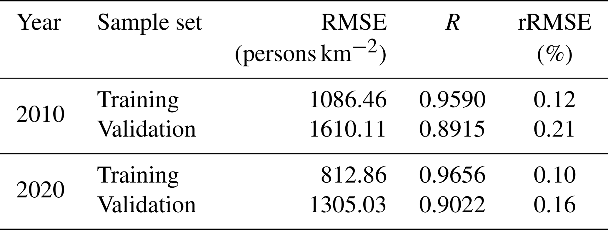
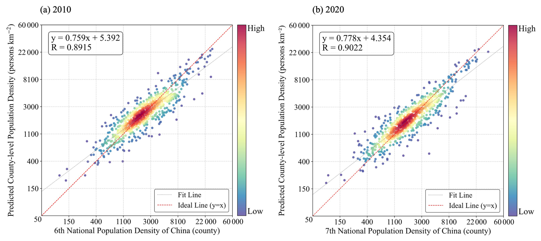
Figure 4 Comparison between predicted and census population densities at the county level for 2010 (a) and 2020 (b).

In terms of error-based metrics, RMSE values for the training datasets were 1086.46 persons km⁻² in 2010 and 812.86 persons km⁻² in 2020, while RMSE values for the validation datasets increased moderately to 1610.11 and 1305.03 persons km⁻², respectively. More importantly, relative RMSE (rRMSE) values for all cases remained below 1 %, indicating that prediction errors account for only a small proportion of the overall population magnitude. This level of relative error is generally considered acceptable and often favourable in large-scale population spatialization studies characterized by substantial spatial heterogeneity. Overall, the combined evidence from correlation analysis, error metrics, and scatter plot diagnostics demonstrates that the proposed XGBoost model achieves both high predictive accuracy and stable generalization performance across different census years. The rigorously calibrated modelling framework therefore provides a reliable foundation for subsequent high-resolution population spatialization and spatiotemporal analysis.

4.1.2 Evaluation for sub-scale estimates

To further evaluate the ability of the trained model to capture finer-scale spatial heterogeneity in population distribution and thereby demonstrate its reliability for gridded population disaggregation, the model was applied to grid-level population estimation and validated against contemporaneous township-level census data, which represent a finer spatial resolution than that used during model training. A total of 10 834 valid township-level population census samples were compiled for 2010 and 10 336 samples for 2020, with a relatively uniform spatial distribution nationwide, providing a robust basis for model assessment and validation.

The consistency between model-derived population estimates and observed township-level census data was evaluated using the Pearson correlation coefficient R. As shown in Fig. 5, the predicted and observed population values exhibit a very strong nationwide agreement. The Pearson correlation coefficient R reaches 0.9013 for 2010 and 0.9246 for 2020, indicating that the model successfully captures fine-scale spatial variability in population distribution beyond the spatial resolution at which it was trained. In addition to the strong correlation, the fitted linear regression line exhibits a slope of 0.991 for 2010 and 0.942 for 2020, which are both very close to the ideal value of 1. This result suggests that the grid-level population estimates are not only highly consistent with township-level census observations in terms of spatial variation, but also largely unbiased in magnitude, despite being trained using coarser county-level population data. In other words, the model preserves population totals and relative differences across township units without systematic overestimation or underestimation.

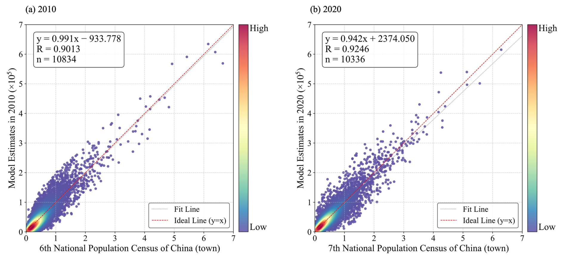
Figure 5 Comparison between predicted and census population counts at the township level for 2010 (a) and 2020 (b).

4.1.3 Evaluation for multi-temporal estimates

To assess the reliability of the multi-temporal population distribution results, the predicted population maps at seven time points from 1990 to 2020 (i.e., 1990, 1995, 2000, 2005, 2010, 2015, and 2020) were systematically validated. Because population estimates for these years were constrained by provincial-level total population counts, model validation was deliberately conducted at the prefecture-level city scale, which represents a finer spatial resolution than the imposed constraint. This evaluation strategy ensures that the validation reflects the robustness and credibility of the spatialized population patterns, rather than merely confirming consistency with the enforced population totals. Specifically, gridded population estimates were spatially aggregated within prefecture-level city boundaries and compared with corresponding city-level population statistics obtained from official statistical yearbooks for the same years. Model performance was assessed using the Pearson correlation coefficient R and linear regression analysis to quantify the strength of agreement and consistency between model-derived estimates and statistical records.

The validation results (Fig. 6 and Table S2) indicate that the model achieves consistently strong performance across all examined time points, with Pearson correlation coefficient R ranging from 0.79 to 0.99. The particularly high correlation coefficients observed for the baseline years 2010 and 2020, approaching 1.0, can be attributed to the modelling design: county-level census population counts were directly used as training targets and subsequently disaggregated to grid cells for these 2 years, such that city-level aggregates of the gridded estimates closely match official city-level statistics. Beyond these baseline years, the model continues to exhibit strong agreement with independent city-level data, indicating that the XGBoost-based framework maintains good temporal stability and spatial generalization capability when extrapolated across multiple decades. Notably, the Pearson correlation coefficient R values display an overall increasing trend over time, suggesting progressively improved predictive performance in more recent years. This improvement is likely driven by the enhanced availability, completeness, and accuracy of building-related and built-up area data in later periods, which provide stronger and more reliable explanatory signals for modelling population distribution dynamics.

Figure 6 Multi-temporal evaluation of AGPC gridded population estimates against city-level population statistics.

It should be noted that the fitting accuracy for earlier periods (e.g., 1990 and 1995) is comparatively lower, which can be primarily attributed to temporal inconsistencies in the input feature data. In this study, several covariates, including topography, road accessibility, and POI density, were assumed to be temporally invariant. However, the POI data were derived from contemporary open platforms and are therefore more representative of recent urban conditions. This mismatch may lead to an overestimation of population weights in certain cities in earlier years, particularly economically developed ones, resulting in a slight overconcentration of population in these areas. In addition, temporal variations in the availability, completeness, and spatial coverage of city-level statistical data across different periods may also contribute to reduced model stability in some regions. Despite the relatively lower accuracy observed for the early years, the multi-temporal population estimates are still able to capture the dominant spatial distribution patterns and long-term temporal evolution of population dynamics. Overall, the model demonstrates strong temporal transferability and produces spatially and temporally coherent results, supporting its applicability for long-term population spatialization analysis.

4.1.4 Comparisons with four existing datasets

To further substantiate the reliability and comparative advantages of the population dataset developed in this study, we conducted a systematic comparison between our gridded population estimates and several widely used population datasets over the same township-level units (Fig. 7). Specifically, our results were compared with three mainstream global gridded population products: GPWv4 (CIESIN, 2018), WorldPop (Tatem, 2017), GHS-POP (Freire et al., 2020), and a recently released China-specific dataset PopSE (Chen et al., 2024), all aggregated to the township-level. As shown in Fig. 7, the Pearson correlation coefficient R value for these four datasets range from 0.7664 to 0.8829 in 2010 and from 0.7590 to 0.9229 in 2020. In contrast, evaluations of our estimates (Fig. 5) indicate consistently higher correlation coefficients in both years (R = 0.9013 in 2010 and R = 0.9246 in 2020), demonstrating improved agreement with township-level census for these two periods.

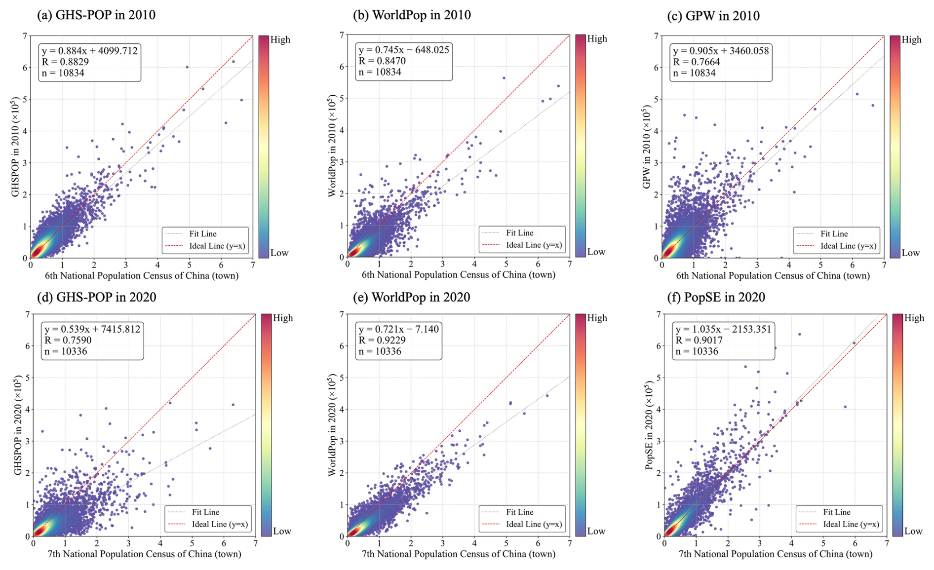
Figure 7 Comparisons among four existing gridded population datasets in 2010 (a–c) and 2020 (d–f) at township-level, including GHSPOP, WorldPop, GPW, and PopSE.

Notably, the regression slopes for GHS-POP (0.539 in 2020) and WorldPop (0.745 in 2010 and 0.721 in 2020) are substantially lower than the ideal value of 1.0. This pattern indicates a systematic underestimation of population totals in township units with high population counts, which are typically associated with highly urbanized and densely built-up areas. Such bias likely reflects the limited capacity of these datasets to capture the exceptionally high population-carrying potential of dense urban environments. Similar underestimation tendencies in high-density urban areas have been documented in previous evaluations of global gridded population datasets (Bai et al., 2018; Chen et al., 2022). By comparison, PopSE exhibits substantially improved agreement with township-level census data in 2020 (R = 0.9017), with a regression slope of 1.035, indicating a more balanced representation across townships with different population sizes. Its strong performance may partly reflect its model development strategy, which incorporated a large number of township-level census records for model training. Nevertheless, AGPC achieves a slightly higher correlation under the same township-level evaluation without using township-level census records for model training, supporting its ability to generalize population patterns from county-level training data to a finer administrative scale.

Table 4 further compares AGPC with the four abovementioned gridded population datasets in terms of RMSE (× 10⁴ persons) and relative RMSE (rRMSE) at the township-level, considering these two metrics together provides a more comprehensive assessment of predictive performance across different population magnitudes. In 2010, AGPC achieves the lowest RMSE (1.8682 × 10⁴ persons) and the lowest rRMSE (16.8 %) among all datasets, slightly outperforming GHS-POP (1.8969 × 10⁴; 17.0 %), and showing clearer improvements over WorldPop (2.3815 × 10⁴; 21.4 %) and GPW (2.9914 × 10⁴; 26.8 %). The advantage is more pronounced in 2020, when AGPC achieves an RMSE of 1.9247 × 10⁴ persons and an rRMSE of 13.7 %, both substantially lower than those of the other datasets. Notably, the rRMSE of AGPC in 2020 is nearly half that of GHS-POP, indicating a marked improvement in scale-adjusted accuracy. Overall, the consistently lower RMSE and rRMSE values indicate that AGPC not only reduces absolute prediction deviations but also maintains better proportional accuracy across township units with varying population sizes.

Table 4 Statistical summary of comparisons among the AGPC and four gridded population datasets at township level.

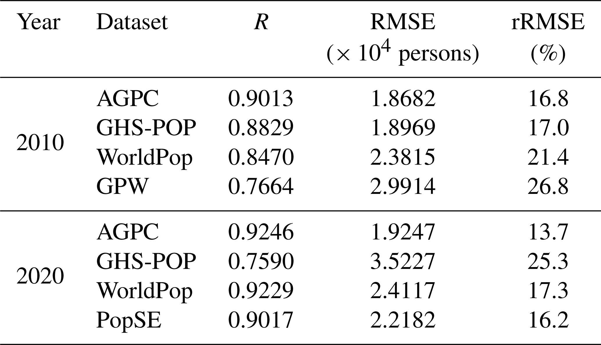
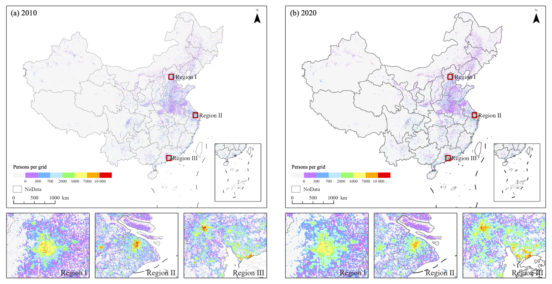
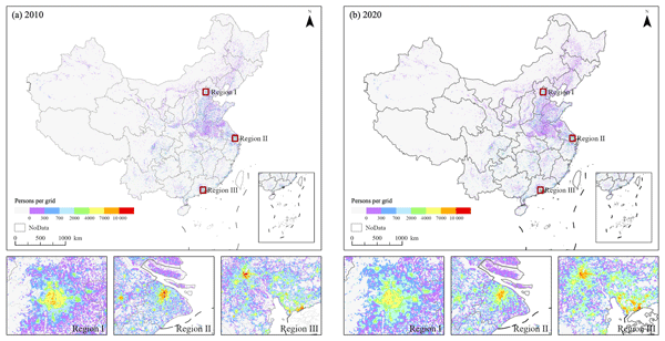
Figure 8 Spatial distribution of AGPC gridded population estimates at 500 m for China in 2010 (a) and 2020 (b).

4.2 Gridded population maps in 2010 and 2020

Building upon the multi-temporal and multi-scale validation results presented above, as well as the comparative evaluation against existing population products, the proposed model demonstrates strong predictive accuracy and robust capability in population spatialization. The trained XGBoost models were therefore applied at the grid level to generate gridded population maps at a spatial resolution of 500 m for 2010 and 2020 (Fig. 8). At the national scale, the derived population distributions for both years successfully reproduce the well-known spatial pattern of population distribution across mainland China. A pronounced east–west gradient is clearly evident, with high population densities concentrated in eastern and coastal regions and markedly lower densities across western plateaus and mountainous areas. Major population agglomerations are observed along the eastern seaboard and within key urban clusters, including the Yangtze River Delta, the Pearl River Delta, and the Beijing–Tianjin–Hebei region, while vast areas of western China remain sparsely populated.

To further demonstrate the model's ability to capture fine-scale spatial heterogeneity, detailed results are presented in the bottom panels of Fig. 8 for three representative urban regions, including Beijing, Shanghai, and the Pearl River Delta urban agglomeration. At the city scale, the spatial distribution of population closely follows the morphology of built-up areas, exhibiting clear spatial clustering patterns. Both Beijing and Shanghai display predominantly monocentric structures, with population density peaking in central urban areas and gradually declining toward peripheral districts, forming distinct radial gradients. In contrast, the Pearl River Delta region presents a markedly different pattern, characterized by a polycentric urban structure with multiple high-density population centres distributed across cities such as Guangzhou, Shenzhen, and Foshan. These spatial patterns are closely associated with regional variations in building volume, urban form, and residential structure. In city centres dominated by dense high-rise development, the predicted population maps exhibit pronounced density peaks, directly reflecting the explicit incorporation of 3D building metrics in the modelling framework.

A comparison between the spatial distributions in 2010 and 2020 further reveals systematic changes in intra-urban population organization across these metropolitan areas. Grid cells characterized by extremely high population densities, which are primarily concentrated in traditional urban cores and highlighted by the highest-density red colour, show a noticeable decline in number over time. In contrast, the spatial extent of grids with moderately high population densities, which are represented by orange colour surrounding the urban centres, expands substantially. This redistribution pattern suggests a gradual shift from highly centralized population concentration towards a more spatially dispersed urban structure. Such a trend is consistent with processes of urban spatial restructuring, including inner-city functional adjustment, housing redevelopment constraints in core districts, and population spillover driven by suburbanization and improved transportation connectivity.

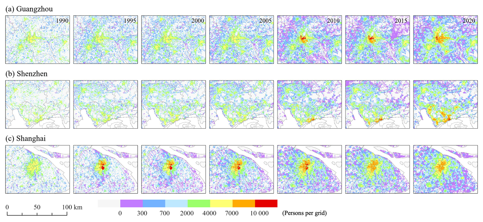
Figure 9 Changes in the spatial distribution of population (persons per grid) in Guangzhou (a), Shenzhen (b), and Shanghai (c) during 1990–2020.

4.3 Multi-temporal population dynamics during 1990–2020

As described in the methodology section, annual gridded population distributions for 1990–2020 were generated by updating time-varying 3D building characteristics and built-up area indicators in the dasymetric model, while constraining total population using annual provincial-level resident population statistics from official yearbooks. To illustrate long-term spatiotemporal dynamics, three representative cities, namely Guangzhou, Shenzhen, and Shanghai were selected to examine changes in population distribution over the past three decades (Fig. 9). These cities reflect distinct urban development trajectories following China's reform and opening up and together capture key stages and structural characteristics of China's urbanization process.

Guangzhou exhibits a gradual transition from a compact monocentric configuration toward a more dispersed, polycentric spatial structure. In the early 1990s, population density was predominantly anchored within the historical urban core. Subsequent decades witnessed a progressive encroachment of high-density grids into peripheral zones, a process characterized by the relative attenuation of hyper-dense centres and a corresponding proliferation of medium-density clusters. Post-2000, intensified suburbanization further catalysed a multi-level hierarchy, where a dominant primary core now coexists with several strategically developing peripheral nodes.

Shenzhen underwent the most radical transformation, evolving rapidly from a singular monocentric footprint into a pronounced polycentric network. Driven by accelerated urbanization, population density diffused swiftly from the nascent core to multiple emerging functional centres. By the mid-2010s, the spatial distribution achieved a high degree of continuity across the metropolitan area. This was achieved through intensive spatial infilling and vertical development, resulting in a seamless landscape of high-density clusters that reflects Shenzhen's unique efficiency in land-use intensification.

Shanghai demonstrates a comparatively stable yet outward-expanding population configuration. While the initial period (1990–2005) was marked by the aggressive polarization of inhabitants into the urban core, the post-2010 era signifies a critical inflection point. During this phase, extreme density peaks underwent stabilization or subtle thinning likely due to urban renewal and decentralization policies, while a pronounced lateral expansion of mid-to-high density grids (4000–10 000 persons per grid) surged towards the periphery. This spatial rebalancing marks a transition from hyper-concentration to a more resilient and balanced polycentric urban form.

4.4 Relative contribution analysis through SHAP

To improve the interpretability of the XGBoost-based dasymetric mapping model, the SHAP framework was employed to quantify the contribution of each feature and characterize its relationship with population density. The SHAP summary plots for 2010 and 2020 (Fig. 10) exhibit generally consistent feature rankings and contribution patterns despite the models being trained independently for the 2 years. Although differences in relative SHAP importance are observed, these values should not be interpreted as direct temporal changes in feature importance. SHAP values quantify the average contribution of each feature to predictions for a specific model and dataset, rather than representing an intrinsic importance of the feature itself. For example, the relative SHAP importance of commercial POI density increases from approximately 28 % in 2010 to more than 35 % in 2020. Because the same POI layer was used for both years, this increase does not necessarily indicate a stronger population dependence on commercial POIs in 2020, but may reflect differences in population distribution, other temporally varying predictors and their interactions, and how the independently trained models utilize these predictors. We therefore focus on the consistency of feature rankings, contribution patterns, and the directionality of SHAP values rather than directly comparing their absolute magnitudes between years.

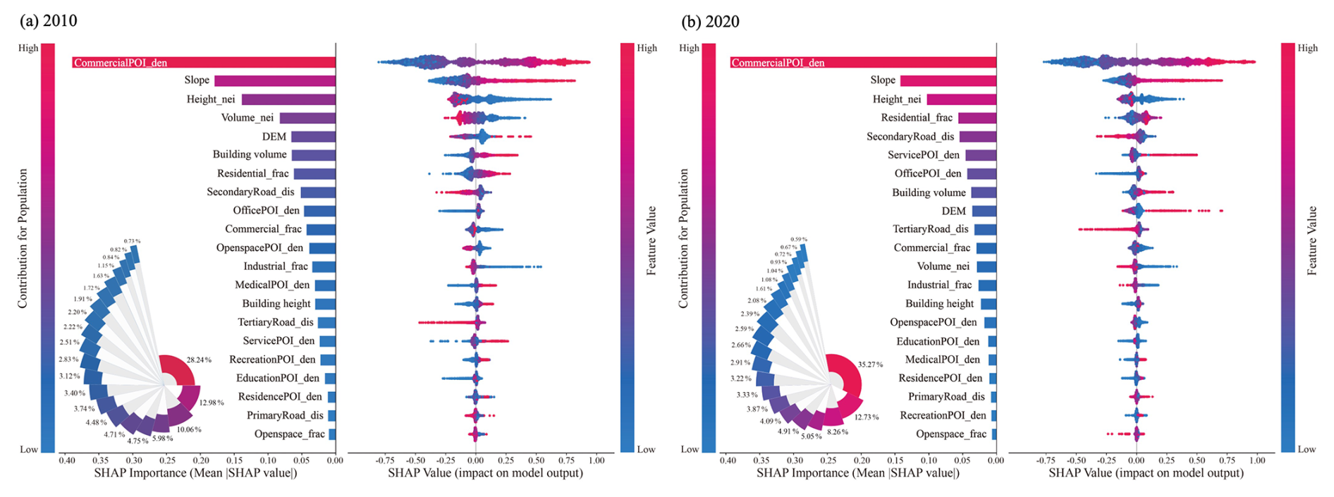
Figure 10 Relative importance of covariates and their directional contributions to model estimation for 2010 (a) and 2020 (b).

Commercial POI density is ranked as the most influential feature in both models, with higher densities consistently associated with positive SHAP values, suggesting a strong relationship between commercial intensity and population concentration. This contribution may partly reflect the high spatial representativeness of commercial POIs, which are generally more comprehensively documented than residential population carriers. Moreover, POI density primarily serves as a proxy for the spatial organization of urban functions rather than a direct indicator of the historical evolution of individual facilities, whose establishment times are often unavailable. Its importance should therefore be interpreted as representing urban functional intensity rather than the temporal development of commercial activities.

In contrast, slope generally exhibits negative SHAP values, implying that steeper terrain constrains population concentration, although a limited number of high-slope samples show positive contributions. 3D building volume consistently ranks among the most influential predictors, with larger building volumes corresponding to positive SHAP contributions. Building-function variables further distinguish different urban land-use characteristics: higher residential building fractions generally increase predicted population density, whereas commercial and industrial building fractions tend to contribute negatively.

These results highlight the importance of incorporating vertical urban morphology and functional characteristics into fine-scale population mapping. The persistent contribution of 3D building volume indicates that population-carrying capacity in dense urban environments cannot be adequately represented by conventional 2D built-up indicators alone. Building-function variables also provide complementary information beyond POI-based indicators. The relatively limited explanatory power of residential POI density may result from the incomplete representation of residential communities in POI datasets despite their dominant role as population carriers. Incorporating building-based functional information therefore helps better characterize residential land use and reduce potential biases in population spatialization.

SHAP dependence plots for the most influential predictors in 2010 (Fig. 11) reveal pronounced nonlinear effects and potential inter-feature interactions in population estimation. Building volume exhibits a clear transition from weakly negative to strongly positive SHAP contributions at approximately 3.0 × 10⁵ m³ per grid, indicating that larger building volumes are associated with increasingly positive contributions to estimated population density beyond this threshold. The colouring by commercial POI density further shows that high commercial POI densities tend to coincide with stronger positive contributions at larger building volumes, suggesting an interaction between vertical built form and commercial activity in the model. Topographic constraints are also evident in the dependence patterns. For comparable building volumes, higher slope values are generally associated with lower SHAP contributions, indicating that steep terrain weakens the positive contribution of building volume to estimated population density. Commercial POI density shows a nonlinear increase in SHAP contribution followed by gradual saturation, with higher residential fractions generally associated with stronger positive contributions, suggesting that mixed-use environments with strong service accessibility constitute key population hubs. Residential fraction itself exhibits a transition from negative to positive contribution at approximately 35 %, while the colouring by building volume further indicates that grids combining high residential fractions with large 3D building volumes tend to have the strongest positive contribution. Together, these patterns highlight the complementary roles of 3D building structure, urban functions, and topographic conditions in the 2010 population estimation model.

Figure 11 Dependence plots of covariates identified by the SHAP summary analysis for 2010.

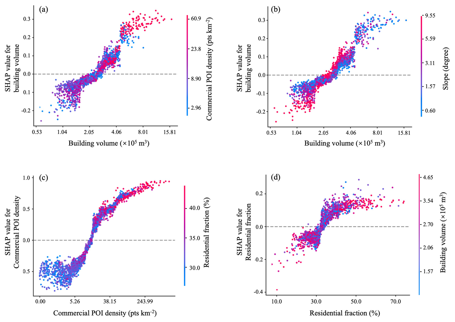
A corresponding set of SHAP dependence plots for the independently trained 2020 model is also provided in the Supplement (Fig. S1). The major dependence patterns are broadly consistent with those identified in the 2010 model: larger building volumes and higher residential fractions are generally associated with positive SHAP contributions, commercial POI density exhibits a nonlinear positive response followed by saturation, and higher slopes tend to weaken the positive contribution of building volume. Interactions between building volume and commercial POI density, as well as between residential fraction and building volume, are also evident in the 2020 model. Although the specific shapes, thresholds, and dispersion of these relationships differ between the 2 years, such differences should not be interpreted directly as temporal changes in the underlying population–environment relationships because the models were trained independently using different population and predictor distributions. The comparison therefore focuses on the broad consistency of contribution directions and response patterns, which collectively highlights the importance of 3D building structure and urban functional characteristics in fine-scale population estimation.

4.5 Effectiveness of 3D building and urban function indicators

To further assess the contribution of 3D building volume and building function features to population spatialization, an ablation-based comparative modelling strategy was adopted. Specifically, we first constructed a baseline dasymetric model using only conventional covariates listed in Table 1, including POI density, proximity to the road network, and topographic variables. The performance of this baseline model was evaluated on both the training and validation datasets. Subsequently, 3D urban environment indicators (e.g., building volume and height) and building function variables were incrementally incorporated into the model. By comparing model performance before and after the inclusion of these features, we quantitatively examined the extent to which 3D building characteristics and functional information improve the accuracy and robustness of population spatialization.

Table 5 Model comparisons when incorporating 3D urban environment and building function variables.

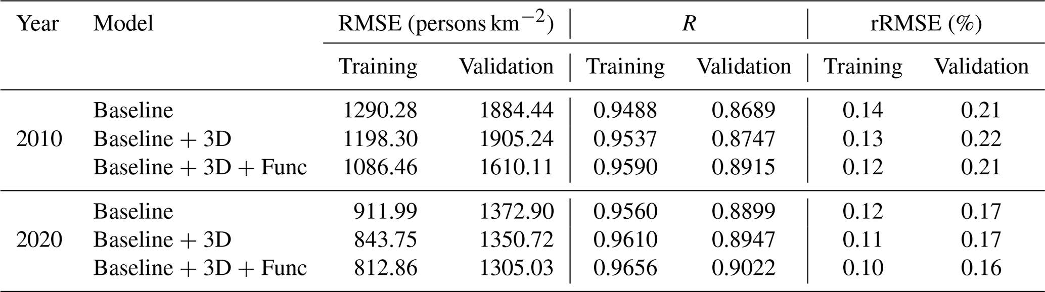
The comparative results (Table 5, Figs. S2 and S3) clearly demonstrate that incorporating 3D urban environment indicators and building function variables leads to substantial performance improvements for both the 2010 and 2020 models. For example, in the 2020 training phase, the inclusion of 3D urban environment indicators reduced the RMSE from 912 (rRMSE: 0.12 %) to 844 persons km⁻² (rRMSE: 0.11 %), while the Pearson correlation coefficient R increased from 0.9560 to 0.9610. Model performance was further enhanced after adding building function variables (RMSE: 813, R: 0.9656, rRMSE: 0.10 %). Similar improvements were observed for the validation results and for the 2010 model, indicating the robustness of these effects across years and datasets. These comparisons confirm that 3D building characteristics provide significant explanatory power in population spatialization by explicitly capturing vertical development and function-specific population-carrying capacity, thereby improving both the accuracy and stability of population distribution estimates.

4.6 3D volume-based vs. 2D-based population estimates

Theoretically, population estimates in the AGPC dataset should show a positive relationship between building volume and population at the 500 m grid level. This is because the model explicitly incorporates the population-carrying capacity implied by 3D building volume and height. Grids with larger building volumes are therefore expected to accommodate more residents. In contrast, gridded population products based solely on 2D built-up coverage, such as WorldPop and GHS-POP, are expected to lose this relationship when built-up coverage approaches saturation. Additional vertical development cannot be captured by these models. This divergence should be most pronounced in regions with strong spatial heterogeneity in building volume.

To test this hypothesis, we selected regions with substantial variation in building volume and compared grid-level population estimates in 2010 across different building volume groups (Fig. 12). Results show that the mean grid-level population in the AGPC dataset increases consistently with building volume, with the strength of this relationship varying by urbanization level. Notably, population estimates continue to rise in high-volume intervals, indicating strong population concentration driven by vertical urban development. In contrast, conventional 2D-based products (WorldPop and GHS-POP) exhibit a different pattern in highly urbanized areas. Population estimates increase with building volume at low to medium ranges, but level off or even decline at higher volumes. This reveals a clear “density saturation” effect, whereby population variation in grids with near-complete building coverage becomes insensitive to further increases in building volume. This limitation reflects the reliance of 2D models on indicators such as built-up coverage and nighttime lights, which cannot represent population aggregation in vertically intensive urban environments. Overall, these comparisons demonstrate that incorporating 3D building volume enables a more realistic and robust representation of population distribution in high-density cities.

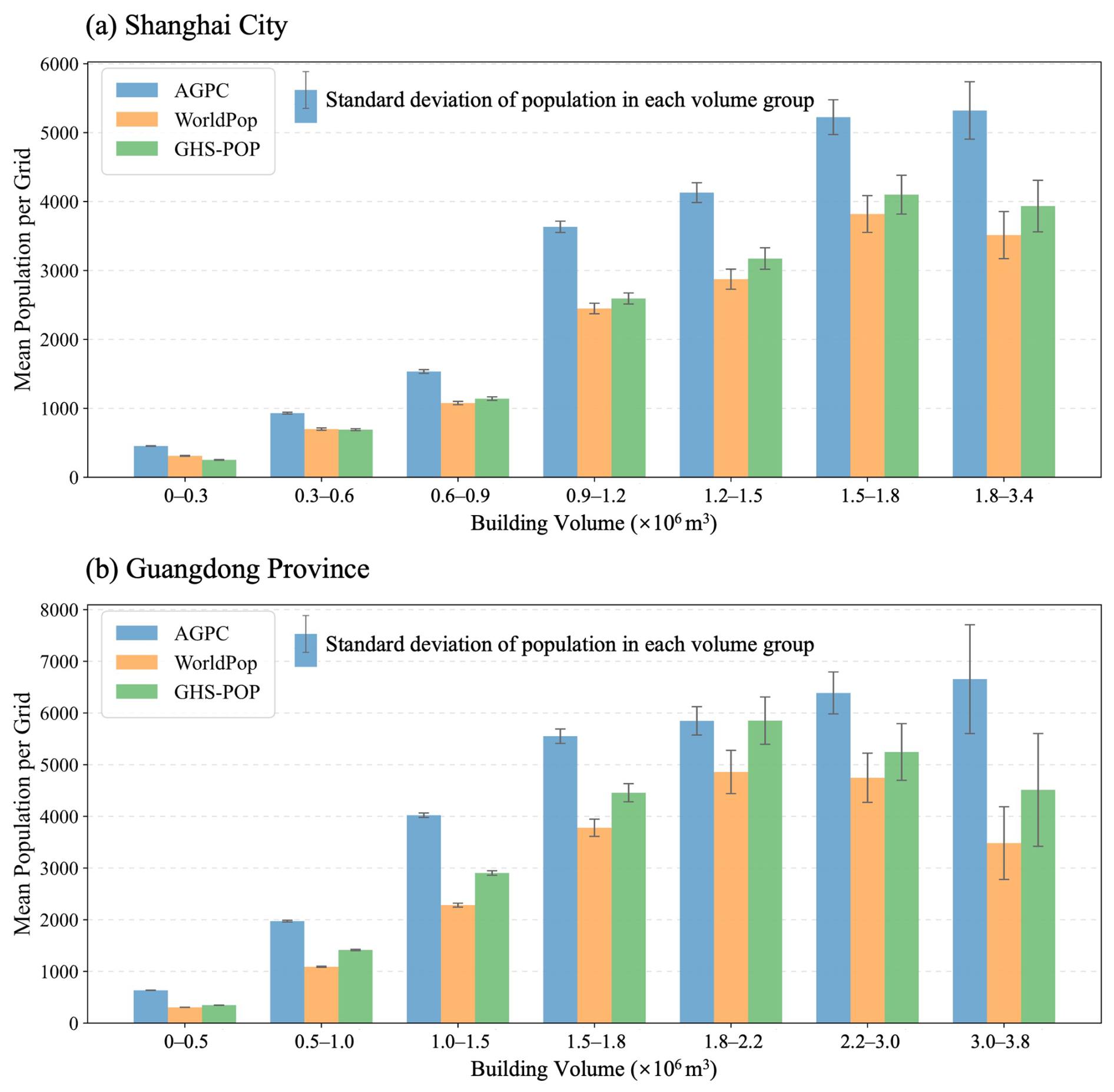
Figure 12 Comparison of gridded population across different building volume groups among AGPC, WorldPop, and GHS-POP in Shanghai (a) and Guangdong Province (b) in 2010.

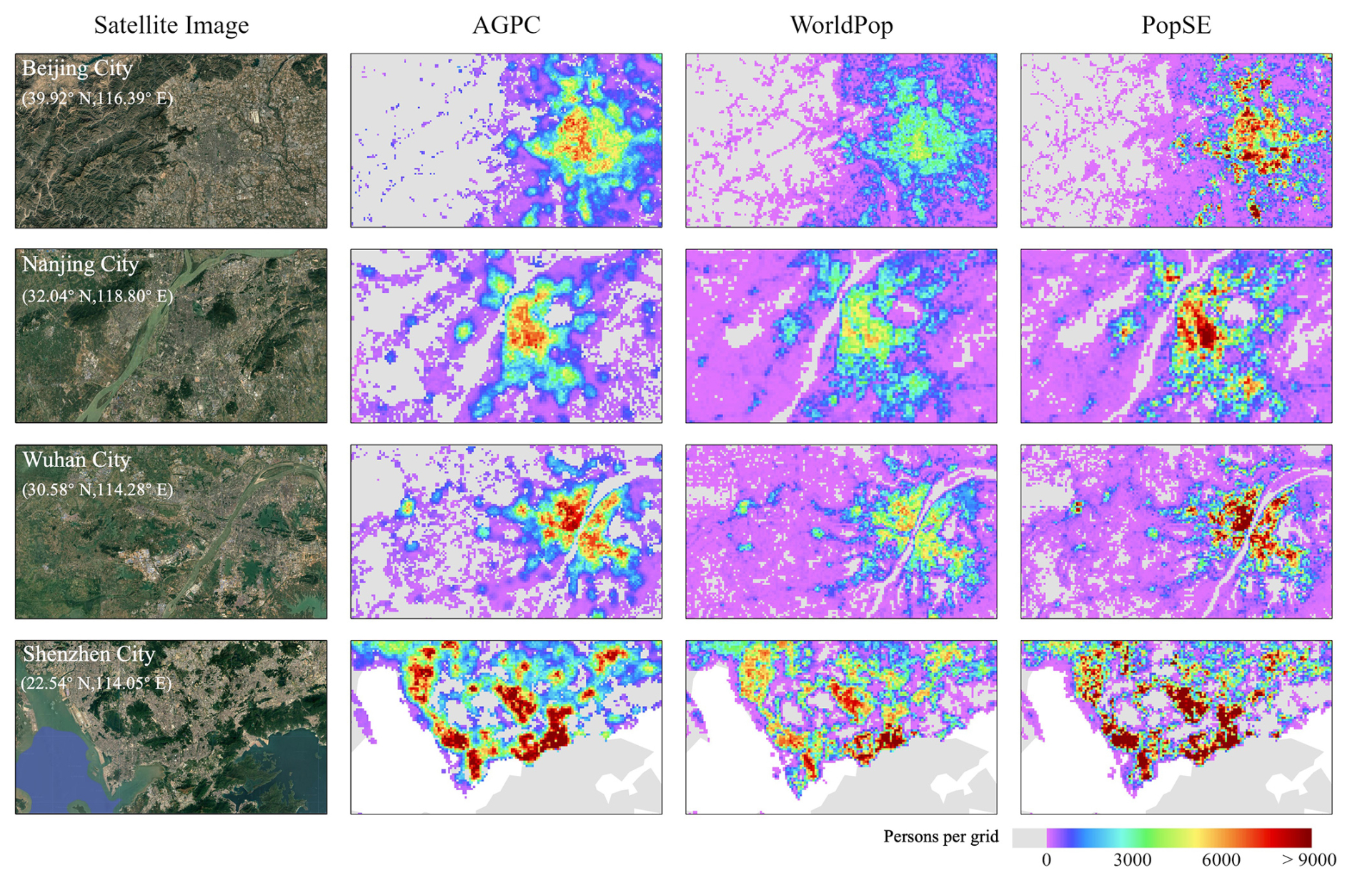
Figure 13 Comparison of gridded population distributions in 2020 among AGPC, WorldPop, and PopSE in selected areas.

To further examine the spatial differences among gridded population products, representative urban regions in Beijing, Nanjing, Wuhan, and Shenzhen were selected for a map-based comparison of population distributions in 2020 (Fig. 13). To ensure comparability across products with different native spatial resolutions, all datasets were aggregated to a common 500 m grid before comparison, thereby minimizing differences arising solely from spatial resolution. Existing products generally show a broader spatial extent of population allocation, with scattered population estimates extending into peripheral regions and sparsely built-up rural areas, whereas AGPC exhibits a closer correspondence between population distribution and the underlying built environment. Within densely developed urban areas, WorldPop tends to produce a smoother population surface, with smaller differentiation among areas characterized by contrasting urban forms and building characteristics. In contrast, AGPC better captures the spatial differentiation of population distribution associated with variations in 3D building structure and building functions, enabling population allocation to more closely reflect differences in population-carrying capacity. Although PopSE also incorporates building-related information, it exhibits stronger localized population concentrations. Some of these high-value clusters appear to correspond more closely to areas of intensive commercial activity than to residential population distribution, suggesting that a stronger influence of commercial activity indicators (e.g., commercial POIs) relative to residential-related information may contribute to such spatial concentration. Overall, these spatial comparisons demonstrate that incorporating 3D urban structure and functional characteristics enables AGPC to provide a more physically informed representation of intra-urban population distribution, particularly in densely developed cities where population concentration cannot be fully characterized by conventional 2D indicators.

4.7 Limitations and future perspectives

Although the proposed AGPC dataset provides spatially and temporally continuous gridded population estimates and outperforms existing products at specific time epochs by explicitly accounting for vertical urban development and function-specific population-carrying capacity, several limitations should be acknowledged. First, some explanatory variables, such as POI density and road network characteristics, were assumed to be temporally static due to the lack of long-term historical datasets. In particular, the POI data were obtained from a consistent 2020 dataset and applied throughout the reconstruction period, which may introduce temporal inconsistency for earlier years. Although POI density primarily represents urban functional intensity and spatial organization rather than the exact historical presence of individual facilities, the lack of temporally consistent historical POI data limits the ability to fully reconstruct past changes in urban functions. This mismatch may cause historical urban functions to be represented by their more recent spatial configuration, potentially affecting fine-scale population allocation in areas that experienced substantial functional transformation or rapid urban development. Nevertheless, historical population changes are also represented by time-varying built-up area and 3D building characteristics and constrained by year-specific statistical population totals, reducing the dependence of the reconstruction on temporally invariant POI information alone. Future studies could integrate multi-temporal POI archives, historical business registration data, or other temporally explicit functional land-use information to better capture the evolution of urban functions and further improve the temporal consistency of population reconstruction. Second, the relationship between covariates and population density was assumed to be identical across county and grid scales. This assumption is potentially affected by the modifiable areal unit problem (MAUP) and may not fully hold at finer spatial resolutions. Similar assumptions are common in previous population downscaling studies, largely because gridded population ground truth data are generally unavailable for model calibration and validation. Third, when reconstructing multi-temporal population dynamics, population weights at the grid level were assumed to change linearly within each 5-year interval, even though annual provincial population totals from official statistical yearbooks were used as constraints. This simplification may smooth short-term population fluctuations driven by abrupt socioeconomic or policy changes.

Looking forward, the proposed framework is readily generalizable and can be extended to other countries and regions worldwide. The incorporation of higher-quality and time-resolved covariates is crucial for further improving gridded population mapping. With the increasing availability of fine-scale datasets, integrating emerging data sources, such as mobile phone signalling data, social media check-in data, and housing rental information, has strong potential to enhance the accuracy and temporal responsiveness of future gridded population datasets.

5 Data availability

The AGPC dataset derived in our study is stored in GeoTIFF format and is freely available at https://doi.org/10.6084/m9.figshare.31338352 (Xu et al., 2026). The GUS-3D dataset used to characterize the spatiotemporal evolution of urban 3D structure is currently accessible through a private link: https://figshare.com/s/9b7d1d40792daa9ab707 (last access: 9 September 2026).

The annual global land-cover dataset AGLC used in this study is publicly accessible through the National Tibetan Plateau Data Center at https://doi.org/10.11888/Terre.tpdc.302477 (Li et al., 2026a).

6 Code availability

The code used for model training, gridded population prediction, and validation for the baseline years is publicly available at Zenodo under https://doi.org/10.5281/zenodo.22671624 (He, 2026). The same workflow was applied separately to the 2010 and 2020 datasets using year-specific inputs and model parameters.

7 Conclusions

This study developed the AGPC dataset, a spatially and temporally consistent gridded population product for mainland China during 1990–2020 at a 500 m resolution, by integrating 3D building volume and building function information into an XGBoost-based dasymetric mapping framework. By explicitly representing the population-carrying capacity of vertically developed urban environments, the proposed approach addresses key limitations of conventional 2D-based population products and improves the characterization of population distribution in dense urban areas. Comprehensive validation across multiple spatial scales demonstrates the robustness and reliability of the proposed model. At the county level, the XGBoost-based framework achieves high predictive accuracy, with Pearson correlation coefficient R value exceeding 0.95 in the training phase and remaining above 0.89 in independent validation, while rRMSE values consistently remain below 1 %. At finer spatial scales, grid-level population estimates aggregated to the township level show strong agreement with independent census data, yielding R values of 0.9013 in 2010 and 0.9246 in 2020, together with regression slopes close to the ideal value of 1.0, indicating both high consistency and minimal systematic bias. Multi-temporal validation further confirms the temporal stability of the AGPC dataset: for seven time points between 1990 and 2020, city-level aggregated estimates exhibit R values ranging from 0.79 to 0.99 when compared with official statistical records, with improved performance observed in more recent years. These results suggest that the model maintains reasonable spatial generalization and temporal transferability despite limited availability of historical covariates.

Comparative analyses with existing population products further highlight the advantages of the proposed approach. AGPC consistently outperforms GPWv4, WorldPop, GHS-POP, and PopSE in terms of Pearson correlation coefficient R as well as RMSE and rRMSE for both benchmark years. More importantly, AGPC preserves a stable and monotonic relationship between population counts and building volume across the full range of urban development intensity. In contrast, conventional 2D population products exhibit clear density saturation effects in high-volume urban environments, leading to systematic underestimation in densely built city centres.

Overall, the results demonstrate that explicitly incorporating 3D building volume and building functional information substantially enhances the accuracy, stability, and interpretability of gridded population estimates, particularly in high-density and vertically developed cities. The AGPC dataset provides a reliable long-term population baseline for China from 1990 to 2020 and offers a scalable methodological framework for population spatialization in other rapidly urbanizing regions. As such, it has broad potential applications in urban studies, environmental assessment, disaster risk analysis, and sustainable development research.