Improving global and regional ocean heat content by consistently combining GRACE gravity, satellite altimetry and Argo profile observations in a joint inversion framework

The current energy imbalance at the top of atmosphere and corresponding heating of the Earth system is the main driver of steric sea level change through ocean heat uptake (OHU). A global constant heat capacity factor is commonly applied to retrieve ocean heat content (OHC) from observed ocean-average steric sea level. We propose an extension to this methodology, which focuses on the leading modes of steric variability, which are derived from an ocean model and fitted to GRACE gravity, satellite altimetry and in situ Argo observations within a joint inversion framework. These modes are utilized to obtain data driven OHC estimates by establishing a mapping between modeled OHC and steric sea level, and rescaling each mode individually based on observed steric sea level change. On global scales for the period January 2005 till December 2024, our OHU results (0.62 W m⁻²) agree well with a variety of published datasets from in situ Argo data, model reanalyses and space-geodetic approaches as well as independent estimates from the CERES project. At basin scales, we demonstrate the global OHU to be driven mainly by warming of the Pacific Ocean (0.23 W m⁻²), followed by contributions from the Indian (0.20 W m⁻²) and Atlantic (0.13 W m⁻²) oceans. Minor contributions are found from the Arctic Ocean (0.01 W m⁻²), the Southern Ocean (0.02 W m⁻²) and the residual ocean (0.03 W m⁻²). Our results also indicate a shift from dominant heating in the Indian Ocean driven by heat transport from the Pacific Ocean, e.g. found during 2005–2015, towards a more evenly distributed global ocean heat budget.

Monthly gridded OHC data from our Grace, Altimetry and Argo Mode Rescaling (GAAMR) method together with corresponding error estimates is available from https://doi.org/10.1594/PANGAEA.994058 (Uebbing and Kusche, 2026).

1 Introduction

Global warming means that the Earth is not in thermal equilibrium; in response mainly to anthropogenic greenhouse gas forcing, volcanic eruptions, solar output variations and internal variability of the climate system. The deviation from the equilibrium can be quantified via the Earth’s Energy Imbalance (EEI). EEI represents the net difference of the in- and outgoing radiation at the top of the atmosphere (Hansen et al., 2011; Trenberth et al., 2014). Over decadal time scales this difference is positive ranging from 0.4–1.0 W m⁻², but at monthly timescales it can fluctuate by several W m⁻² (Loeb et al., 2021). Measurements of EEI obtained from satellite radiometers within the CERES project (Wielicki et al., 1996) have improved our understanding of the global climate system, and of the energy exchange between the atmosphere, the ocean, the cryosphere, and the land surface. They represent an important metric for evaluating climate models. However, being a small residual of large fluxes – globally averaged solar irradiance at the top of the atmosphere amounts to about 340 W m⁻² (Loeb et al., 2009) – EEI is difficult to measure in this way.

The current understanding is that heat uptake in the global ocean (OHU) is responsible for about 90 % of EEI (von Schuckmann et al., 2020), and that shallow ocean layers (upper 700 m) contribute to OHU by about 65 %, the depth layer between 700–2000 m about 20 %, and the abyssal ocean about 15 % of this (Gleckler et al., 2016). More recent estimates by Pan et al. (2025) find 64 %, 29 % and 7 % for the same depth layers, respectively.

While the ocean absorbs heat almost entirely via the air-sea interface, the horizontal and vertical rearrangement of heat is controlled by winds, ocean currents and the level of stratification and mixing in the ocean. The steady-state is that excess heat absorbed in the tropics is transported by ocean currents to extra-tropical regions (Bryden and Imawaki, 2001; Trenberth and Caron, 2001; Ferrari and Ferreira, 2011). Patterns of anomalous heat uptake then vary at seasonal and inter-annual time scales in the upper ocean, with ‘marine heat waves’ sometimes responding to anomalous air temperatures, while it is believed that the deep ocean reacts much slower to atmospheric variability (e.g., Holbrook et al., 2019; Amaya et al., 2023). However, heat uptake in the deeper ocean is much more difficult to measure and model and, thus, more uncertain. Recent observational studies have suggested a strong hemispheric asymmetry in anomalous ocean warming over the modern period where the ocean is sampled down to 2000 m by autonomous floats (Durack et al., 2018), with the Southern hemisphere responsible for 0.6×10²²–0.7×10²² J yr⁻¹ corresponding to about 0.4 W m⁻² with respect to the total Earth's surface, and only 0.13×10²²–0.36×10²² J yr⁻¹ (0.1–0.2 W m⁻²) for the Northern hemisphere between 2007 and 2015 (Durack et al., 2018). Persistent patterns of warming have been identified for the Southern Ocean, but also in the North Atlantic a warming in the subtropics off the east coast of Canada is found, with cooling northward of 40° latitude (Zhang, 2008; Caesar et al., 2018).

Ocean warming can lead to increased stratification (Li et al., 2020), thus, preventing mixing of water masses, changes in current regimes, expansion of oxygen depleted zones affecting marine ecosystems, and increased melting of marine-terminating glaciers. It is currently unclear to what extent deep-sea ecosystems and, e.g. corals, will be affected by warming temperatures and related factors such as acidification and oxygen depletion (Portilho-Ramos et al., 2022). Due to ocean thermal expansion, warming of the ocean contributes about 42 % of current global mean sea level rise since 1993 (WCRP-Global-Sea-Level-Budget-Group, 2018), although at regional scales the warming can dominate the sea level budget with up to 75 % (Rietbroek et al., 2016). On relatively short timescales (2005–2013), halosteric changes are believed to have only a secondary effect on regional sea level change for most of the world (Llovel and Lee, 2015). Long-term halosteric freshening effects that add to the thermosteric expansion are found for the Pacific Ocean while the Atlantic Ocean becomes more saline and, thus, compensates the thermosteric change to a certain extend (Durack et al., 2014). Quantifying OHU via measuring thermal expansion is generally achieved either from in situ temperature profiles observed by Argo floaters freely drifting in the ocean (Roemmich et al., 2009), or from geocentric sea level measured by satellite altimetry while removing ocean mass change derived from satellite gravimetry (e.g., Rietbroek et al., 2016; WCRP-Global-Sea-Level-Budget-Group, 2018; Horwath et al., 2022).

At regional scales, ocean heat storage changes due to radiation imbalance at the surface and due to changes in heat transport; i.e. heat redistribution within the ocean. While heat addition through the surface dominates in the global average, horizontal ocean heat redistribution results in important regional contributions, especially in the tropics (Dias et al., 2020). This ocean heat redistribution is made up predominantly by changes in horizontal ocean circulation, with additional but minor effects stemming from changes in vertical water mixing. Heat transport within the ocean is mostly from the tropical ocean toward the poles driven by overturning, gyres, eddies or diffusion (Jia, 2003). These pathways of heat storage change have been extensively studied in ocean and coupled ocean-atmosphere simulations, but it is difficult to quantify their contribution at regional scale. Ocean reanalyses seek to assimilate ample remote sensing and in situ ocean observations, but deviations between models are still large (Palmer et al., 2017).

Geocentric sea level has been continuously monitored since 1993 from the Topex/Poseidon spacecraft and its successor Jason-1/-2/-3 and Sentinel-6 missions resulting in a time series of, nowadays, more than 30 years of radar altimetry observations between ±66° latitude with a 10 d interval (International-Altimetry-Team, 2021). In addition, other altimeter missions have been launched reaching higher latitudes and better spatial coverage at the cost of a longer repeat interval, but still augmenting the reference mission dataset. Radar altimetry is a mature technique and rates of absolute sea level, when averaged over regional oceans, are accurate at 0.3 mm yr⁻¹ level (International-Altimetry-Team, 2021). This accuracy is mostly driven by accounting for the effect of glacial isostatic adjustment, in addition to orbit errors and those of the remaining atmospheric and geophysical correction effects. Since 2002 the Gravity Recovery and Climate Experiment (GRACE, Tapley et al., 2004) and its successor GRACE follow-on (GRACE-FO, Kornfeld et al., 2019) enable observation of time-variable gravity changes and, thus, ocean mass change, on a monthly basis. Steric sea level changes can be inferred from either combining altimetry measured variations with GRACE-observed ocean mass changes or by converting in situ profiles of temperature and salinity. The latter are observed by a globally distributed array of freely drifting floats in the ocean as part of the Argo program (Roemmich et al., 2009). Full global coverage from several thousand Argo floats has been achieved since 2005 providing in situ profiles of the upper 2000 m of the ocean about every 10 d.

Combining geocentric sea level observed from satellite altimetry, monthly steric sea level change derived from in situ Argo profiles together with ocean mass changes derived from GRACE(-FO) gravimetry are used to estimate sea level budgets. In other words, a sea level budget represents the partitioning of total sea level change into mass and steric (volumetric) components (e.g., Rietbroek et al., 2016; WCRP-Global-Sea-Level-Budget-Group, 2018; Meyssignac et al., 2019; Uebbing et al., 2019; Hakuba et al., 2021; Horwath et al., 2022). It is then possible to infer information on ocean heat content (OHC) change by converting from the (thermo-)steric to the OHC domain based on the global mean thermal expansion efficiency of heat, typically derived from an ocean reanalysis (Russell et al., 2000; Marti et al., 2022). This simple scaling by applying a globally constant factor for converting (thermo-)steric sea level rates to estimates of OHU has been widely established over the past years (Meyssignac et al., 2019; Hakuba et al., 2021). However, the expansion efficiency of heat is not globally constant, neither on spatial, nor temporal scales, which makes it difficult to apply for regional analyses. In addition, uncertainties of the involved sea level parameters are significantly larger compared to their respective global averages, which might add to the uncertainty of OHC at regional scale. Recently, extensions to this approach have been published by converting space-geodetic steric sea level on individual grid points, while computing the individual conversion factors based on in situ Argo data (Marti et al., 2022, 2024).

Here, we propose a two-step solution to this problem. In the first step, we derive sea level budgets from a global fingerprint inversion approach (Rietbroek et al., 2016; Uebbing et al., 2019). For this, we derive mass and steric related spatial patterns, so called fingerprints (see Sect. 2), which are then fitted to GRACE(-FO), in situ Argo profiles and along-track satellite altimetry data in order to estimate scaling factors for each individual fingerprint on a monthly basis. Combining the estimated scale factors with the corresponding fingerprints then allows for construction of global and regional sea level budgets. In a second step, we project OHC extracted from an ocean reanalysis onto the same steric fingerprints serving as an orthonormal basis, thus, computing corresponding OHC scale factors. In this study, we selected the ORAS5 reanalysis (Zuo et al., 2019) as a basis for the fingerprint computation and deriving OHC. Modes of OHC are rescaled, i.e. adjusted to satellite observations, based on the factors found from the sea level inversion estimation (see Sect. 2) allowing to reconstruct rescaled monthly gridded OHC; this combines the benefits of high spatial resolution from the ORAS5 model-derived spatial information with observation-based temporal information from the inversion procedure. The resulting monthly grids of OHC can then be further analyzed on global and regional scales. In the following, our novel method will be denoted as GRACE, Argo and Altimetry based Mode Rescaling (GAAMR) approach.

2 Data and Methods

2.1 Principal Component Analysis (PCA)

A p×n data matrix H containing modeled steric sea level or OHC data on p grid points and n monthly observations or model data, can be analyzed by finding the best fitting linear combination of defined base functions, which represent the data in its entirety using PCA (Preisendorfer, 1988; Jolliffe and Cadima, 2016); also known as EOF decomposition. The data matrix, H, can be decomposed using singular value decomposition as follows

$${\displaystyle }\mathbf{H}={\mathbf{USV}}^{\mathrm{T}},$$

where S is of size p×n and contains, at most $m=min(p,n)$, distinct singular values s_i on its main diagonal. The columns of U represent the time-invariant eigenvectors and are generally referred to as empirical orthogonal functions (EOF)s or “modes”. Corresponding principal components (PC)s, D, are then computed from D=SV^T. These can be interpreted as the temporal evolution of scaling factors needed to reconstruct the input data, H, from the orthonormal basis, U, defined by the EOFs.

2.2 Steric Sea Level from Ocean Reanalysis and In Situ Profile Data

Model based steric sea level from the ORAS5 reanalysis is used as a basis for extracting leading EOFs for estimating sea level budgets as part of the fingerprint inversion. Similarly, in situ temperature and salinity profiles obtained from the Argo program (Roemmich et al., 2009) are processed to global gridded products by various institutions using optimal interpolation techniques (e.g., Zhang et al., 2022). For both, model and in situ based datasets, steric sea level anomalies relative to a reference steric sea level are computed from the 4D temperature, T, and salinity, S, data as the integral of the ratio of density differences relative to the reference density, ρ_ref, up to maximum depth, H, given by (Gill and Niller, 1973; Landerer et al., 2007)

$$\begin{array}{}\text{(1)}& {\displaystyle }\begin{array}{rl}& h_{\text{steric}}(\mathit{\lambda },\mathit{\varphi },t)=\\ & \underset{-H}{\overset{\mathrm{0}}{\int }}{\displaystyle \frac{\left\{\begin{array}{c}{\mathit{\rho }}_{\text{ref}}\left(T_{\text{ref}}\right(\mathit{\lambda },\mathit{\varphi },z),S_{\text{ref}}(\mathit{\lambda },\mathit{\varphi },z),p(\mathit{\lambda },\mathit{\varphi },z\left)\right)\\ -\mathit{\rho }\left(T\right(\mathit{\lambda },\mathit{\varphi },z,t),S(\mathit{\lambda },\mathit{\varphi },z,t),p(\mathit{\lambda },\mathit{\varphi },z,t\left)\right)\end{array}\right\}}{{\mathit{\rho }}_{\text{ref}}\left(T_{\text{ref}}\right(\mathit{\lambda },\mathit{\varphi },z),S_{\text{ref}}(\mathit{\lambda },\mathit{\varphi },z),p(\mathit{\lambda },\mathit{\varphi },z\left)\right)}}\mathrm{d}z,\end{array}\end{array}$$

where the density, ρ, is derived from temperature, salinity and pressure, p following the Thermodynamic Equation Of Seawater – 2010 (TEOS-10, IOC et al., 2010). In case of the ORAS5 model, H represents the maximum model depth of ∼6000 m, while when we analyze Argo data, a depth of 700 m is used. In other words, the integral limits are adapted depending on the utilized data, e.g. model or Argo, throughout the manuscript.

2.3 Fingerprint Inversion Method

The global fingerprint inversion method fits spatial sea level patterns, so called “fingerprints”, to a combination of space-geodetic datasets from satellite altimetry and GRACE(-FO) gravity data in a forward modeling least-squares sense (Rietbroek et al., 2016; Uebbing et al., 2019). The fingerprints refer to individual mass and steric contributions to sea level and are constructed based on a priori information. Here, we employ an updated inversion method (Uebbing, 2022), which is summarized in the following.

2.3.1 Sea Level Fingerprints

Sea level contributions include the mass imbalance from melting of land glaciers and the ice sheets in Greenland and Antarctica, terrestrial hydrology mass fluxes, as well as internal ocean mass variations. In total we fit 486 fingerprints, subdivided into 236 mass and 250 steric fingerprints, to the input data. The 236 mass patterns represent the passive ocean response derived from solving the sea level equation (Woodward, 1888; Farrell, 1972; Rietbroek et al., 2016) relating variations from a predefined land load to corresponding changes in sea level. Land glacier positions for 68 glacier regions have been extracted from the Randolph Glacier Inventory (RGIv6.0, RGI Consortium, 2017). The Greenland contribution is split into 16 sub-basins based on Wouters et al. (2008) and augmented by ice altimetry derived melting rates (Strößenreuther et al., 2020) for better mass localization. Similarly, the 27 basins for Antarctica (Zwally and Giovinetto, 2011) are also augmented by ice altimetry melting rates (Schröder et al., 2019). For the ice melting related patterns, these are directly processed utilizing the sea level equation. For the terrestrial hydrology contribution, first, PCA is performed on WaterGAP Hydrological Model (WGHMv2.2e, Müller Schmied et al., 2024) utilizing data from 2003.0 till 2020.0 where the 75 retained EOFs represent about 80 % of the modeled variance. For the corresponding hydrological EOFs, so far only defined over land, we then further derive the related ocean fingerprints by applying the sea level equation. Internal mass variations (IMV) are characterized by transports of water masses within the ocean without external influx from land. Model based IMV is commonly removed during GRACE(-FO) level 2 processing, but has to be restored as part of computing ocean mass change (Uebbing et al., 2019). We co-estimate IMV as an individual sea level component based on auxiliary data extracted from the AOD1B-GAB model product (Dobslaw et al., 2017), defined only over the ocean, where the 50 dominant modes have been extracted using PCA.

Steric fingerprints are constructed from first converting monthly 4D reanalysis datasets of temperature and salinity to steric sea level change based on the Ocean Reanalysis System 5 (ORAS5, Zuo et al., 2019). This is done for a depth level of 0–700 m as well as a deep ocean part (below 700 m). For the halosteric effect, both depth level datasets are corrected for artificial trend effects resulting from assimilation of non-global coverage Argo data before 2005 and to account for salinity drifts after 2015 due to an Argo buoy manufacturing problem (Wong et al., 2023). This is done by enforcing the global halosteric trend to be zero during the GRACE(-FO) era before EOF decomposition. Dominant EOFs of thermo- and halosteric sea level change are then extracted for both depth regions by employing PCA. The seasonal signal has not been removed beforehand since the observational data also includes the seasonal information. As these do not represent changes in ocean mass, the modes can be utilized directly as fingerprints without further applying the sea level equation. For the upper ocean, 150 modes (75 each for thermo- and halosteric variations) representing about 80 % of the modeled variance are used, while only the first 50 EOFs for thermo- and halosteric changes are used for the deep ocean; these represent generally less than 80 % signal variations as we do not completely trust the high frequency deep ocean signals present in the model data. Despite the deep ocean steric contribution not being directly constrained by observations, it can still be derived from the combination of altimetry, GRACE(-FO) and upper 700 m steric information.

Here, we focus on ORAS5 reanalysis data as a basis for our steric fingerprints due to the higher spatial resolution and since it is additionally constrained by ocean observations via data assimilation. When we vary the utilized spatial patterns for the overall steric contribution, e.g., with those of a non-assimilated version of the Finite Element Sea-ice Ocean Model (FESOM, Timmermann et al., 2009), we obtain steric rates in good agreement within uncertainty ranges with those derived based on ORAS5 and reported in this study (Uebbing, 2022). Similarly, variations in other aspects, such as different GRACE(-FO) products or GIA corrections lead only to small variations of a few percent in our inversion-based steric sea level estimates.

2.3.2 Inversion Input Data

Fingerprints are fitted to satellite altimetry and GRACE(-FO) observations in order to separate individual mass and steric contributions and estimate monthly scaling factors, x, for the time-invariant fingerprints. All corrections applied to the observations, such as GIA corrections etc., are consistently selected across all datasets. Along-track satellite altimetry sea level anomalies, h_SLA, are extracted from the Radar Altimetry Database System (RADS, Scharroo et al., 2013) for all available altimetry missions between January 2002 and December 2024 with 1 Hz sampling, representing about 5 km along-track segments on the ground.

$$\begin{array}{}\text{(2)}& {\displaystyle }\left[\begin{array}{c}{h}_{{\text{SLA}}_{\mathrm{1}}}\\ \mathrm{⋮}\\ h_{{\text{SLA}}_J}\end{array}\right]={\mathbf{A}}_{\text{altim}}\left[\begin{array}{c}{\mathit{x}}_{\text{ice}}\\ {\mathit{x}}_{\text{glac}}\\ {\mathit{x}}_{\text{hydr}}\\ {\mathit{x}}_{\text{steric}}^{\text{700\hspace{0.17em}m}}\\ {\mathit{x}}_{\text{steric}}^{\text{deep}}\\ {\mathit{x}}_{\text{IMV}}\end{array}\right]+{\mathit{e}}_{\text{altim}},\end{array}$$

where the matrix A_altim includes the individual fingerprints of geocentric sea level evaluated at the along-track altimetry positions in its columns. The stochastic model for the altimetry input data contains the 1 Hz variances on the diagonal of the covariance matrix, generally with magnitudes of ∼7 cm extracted from RADS, while assuming individual 1 Hz measurements to be uncorrelated. We prefer using along-track altimetric data over gridded products, since not all grid points are observed regularly and gaps in these products need to be filled, which would introduce another unnecessary potential source of error into our inversion.

GRACE(-FO) input data consists of full spherical harmonic normal equation systems from the ITSG-2018 gravity field (Mayer-Gürr et al., 2018; Kvas et al., 2019) up to degree and order 120, which corresponds to a spatial resolution of about 300 km. Corresponding observational equations describe the relation between the spherical harmonic and fingerprint domains

$$\begin{array}{}\text{(3)}& {\displaystyle }\left[\begin{array}{c}a\mathit{\delta }{c}_{\mathrm{20}}\\ \mathrm{⋮}\\ a\mathit{\delta }{c}_{nm}\end{array}\right]={\mathbf{A}}_{\text{grav}}\left[\begin{array}{c}{\mathit{x}}_{\text{ice}}\\ {\mathit{x}}_{\text{glac}}\\ {\mathit{x}}_{\text{hydr}}\\ {\mathit{x}}_{\text{IMV}}\end{array}\right]+{\mathit{e}}_{\text{grav}},\end{array}$$

where multiplication with the Earth radius, a, converts the Stokes coefficients, δc_nm, to geoid heights and the columns of matrix A_grav contain the individual mass fingerprints expressed as geoid heights in spherical harmonics. The stochastic model of the gravity input data considers the full covariance matrix provided for the ITSG2018.

In order to constrain the steric part of the sea level budget, we employ in situ temperature and salinity profile data observed at P positions by the Argo programme (Roemmich et al., 2009) for each month. These have a resolution of about 1° globally, but their density varies regionally (Fig. B3). Here, we utilize data from the easyCORA dataset (Szekely et al., 2019), which includes a collection of various types of in situ temperature and salinity measurements. We limit our data to the depth profiles observed by Argo. These are then converted to steric sea level, $h_{{\text{steric}}_p}$, following Eq. (1) based on the thermodynamic equation of seawater (IOC et al., 2010). These steric sea level variations are then introduced as observations and fitted to the steric fingerprints as

$$\begin{array}{}\text{(4)}& {\displaystyle }\left[\begin{array}{c}{h}_{{\text{steric}}_{\mathrm{1}}}\\ \mathrm{⋮}\\ h_{{\text{steric}}_P}\end{array}\right]={\mathbf{A}}_{\text{steric}}\left[\begin{array}{c}{\mathit{x}}_{\text{steric}}\end{array}\right]+{\mathit{e}}_{\text{steric}}.\end{array}$$

Similar to above, the matrix A_steric includes the individual steric fingerprints evaluated at the P Argo profile positions in its columns and the vector e_steric represents the stochastic information. The steric errors are derived from a Monte-Carlo simulation (e.g., Binder and Heermann, 2010) varying the observed data according to their formal errors and computing the corresponding steric height estimates. While simply propagating the formal errors would lead to very small errors in the sub-millimeter level, the Monte-Carlo approach provides more realistic errors in the centimeter range.

2.3.3 Estimation of Inversion Results

Monthly normal equation systems are constructed for GRACE(-FO), in situ Argo and each altimetry mission based on the deterministic and stochastic models introduced above. These are then combined using variance component estimation (Koch and Kusche, 2002) resulting in combined normal equation systems, which can then be solved by least squares estimation for the monthly scaling factors, x, for each fingerprint as well as the corresponding error covariance Σ_xx. We select 0.25° resolution to evaluate all our fingerprints, based on the highest available spatial resolution of the model data used from constructing those fingerprints. Afterwards, we reconstruct total sea level change or individual contributions, e.g. steric sea level, from the linear combination of the respective fingerprints with the corresponding estimated scale factors. These monthly maps of sea level change together with their propagated errors can then be further analyzed in terms of global and regional sea level budgets (Rietbroek et al., 2016; Uebbing et al., 2019; Uebbing, 2022; Willen et al., 2026).

2.4 Space Geodetic Approach for Converting Steric Sea Level to Ocean Heat Content

2.4.1 Classic Approach: Directly converting steric sea level

As mentioned above, the majority of the excess heat originating from TOA-EEI is warming the world's oceans entailing expansion of the water column and, thus, steric sea level change observable by space geodetic techniques (e.g., Meyssignac et al., 2019; von Schuckmann et al., 2020; Hakuba et al., 2021; Marti et al., 2022, 2024).

Globally, conversion between (thermo-)steric sea level change and OHC has been defined by Russell et al. (2000) as the ratio between the derivative of the specific volume with respect to temperature, ${\mathit{\nu }}_{T_i}$ [m³ (kg C)⁻¹], and the specific heat capacity, c_p [J (kg C)⁻¹], multiplied with the ocean area, A_oce, resulting in the expansion efficiency of heat, ϵ usually reported in units of m YJ⁻¹, e.g. 0.121 ± 0.015 m YJ⁻¹ (Hakuba et al., 2021), given by

$$\begin{array}{}\text{(5)}& {\displaystyle }\mathit{ϵ}={\displaystyle \frac{{\mathit{\nu }}_{T_i}}{c_p{A}_{\text{oce}}}}.\end{array}$$

When we compute a global average value based on ORAS5 model reanalysis data, we find 0.52 $\mathrm{W}{\mathrm{m}}^{-\mathrm{2}}(\mathrm{mm}{\mathrm{yr}}^{-\mathrm{1}}{)}^{-\mathrm{1}}$, which agrees well with published literature values (e.g., Meyssignac et al., 2019; von Schuckmann et al., 2020; Hakuba et al., 2021). Alternatively on global scales, ϵ can be derived by dividing estimates of (thermo-)steric sea level change by corresponding OHC change estimates (Meyssignac et al., 2019; Hakuba et al., 2021). In order to facilitate more regional approaches for converting steric sea level derived from combining GRACE and altimetry data, it is possible to compute this conversion factor regionally by utilizing in situ Argo profiles (Marti et al., 2022, 2024) or model data; in this study we utilized ORAS5 for directly converting regional steric sea level from the inversion approach.

2.4.2 GRACE, Argo and Altimetry based Mode Rescaling (GAAMR) Approach

Leveraging the inversion setup and the estimated time-variable scaling factors x, it is possible to derive improved global and regional observation-driven OHC by expanding on the widely applied approach of scaling steric data with only one factor as described above. Instead, the idea is to utilize the separation of steric sea level into individual modes within the inversion setup in order to rescale these separately, while at the same time accounting for differences in (thermo-)steric and OHC signals to a certain extent.

Starting from the steric EOFs, U_ster, which are derived from a priori model reanalysis (thermo-)steric sea level, we also have corresponding model PCs, D^(ster-mod), available. In addition, fitting the fingerprints to the altimetry, Argo and GRACE(-FO) data results in observation-driven estimates, D^(ster-inv). Assuming similar spatial structures between thermosteric sea level change and OHC, we then project modeled OHC onto the same orthonormal and unitless basis, U_ster, in a least-squares sense in order to derive PCs, D^(ohc-mod) from

$$\begin{array}{}\text{(6)}& {\displaystyle }{\mathbf{D}}^{\left(\text{ohc-mod}\right)}=({\mathbf{U}}_{\text{ster}}^{\mathrm{T}}{\mathbf{U}}_{\text{ster}}{)}^{-\mathrm{1}}{\mathbf{U}}_{\text{ster}}^{\mathrm{T}}{\mathbf{Q}}^{\left(\text{mod}\right)}.\end{array}$$

Since U_ster is interpreted as unit-less, the resulting scaling factors, D^(ohc-mod), will have the same units as OHC. Here, we chose the ORAS5 model (Zuo et al., 2019) for both the steric sea level data as well as the modeled OHC, Q^(mod).

In a next step, one could simply scale the model OHC ${\mathit{d}}_j^{\left(\text{ohc-mod}\right)}$ for each individual mode j based on the ratio of the inversion estimated and observation driven steric sea level change according to

$$\begin{array}{}\text{(7)}& {\displaystyle }{\stackrel{\mathrm{̃}}{d}}_j^{\left(\text{ohc-resc}\right)}\left(t\right)={\displaystyle \frac{d_j^{\left(\text{ster-inv}\right)}\left(t\right)}{d_j^{\left(\text{ster-mod}\right)}\left(t\right)}}{d}_j^{\left(\text{ohc-mod}\right)}\left(t\right).\end{array}$$

Writing the rescaling this way is possible for each point in time, t, by computing the element-wise ratio between $d_j^{\left(\text{ster-inv}\right)}\left(t\right)$ and $d_j^{\left(\text{ster-mod}\right)}\left(t\right)$, yielding monthly scaling factors for each mode j. However, numerical problems may arise in case the steric model PC, $d_j^{\left(\text{ster-mod}\right)}\left(t\right)$, is close to zero since anomalies of steric sea level and OHC are utilized. This is a similar problem as discussed in Marti et al. (2022), who then resorted to full quantities. Here, we circumvent the numerical problems by modifying the conversion (Eq. 7) as follows

$$\begin{array}{}\text{(8)}& {\displaystyle }\begin{array}{rl}{\stackrel{\mathrm{̃}}{d}}_j^{\left(\text{ohc-resc}\right)}& \left(t\right)=d_j^{\left(\text{ohc-mod}\right)}\left(t\right)\\ & +{\displaystyle \frac{\Vert {\mathit{d}}_j^{\left(\text{ohc-mod}\right)}\Vert }{\Vert {\mathit{d}}_j^{\left(\text{ster-mod}\right)}\Vert }}\left(d_j^{\left(\text{ster-inv}\right)}\right(t)-d_j^{\left(\text{ster-mod}\right)}(t\left)\right).\end{array}\end{array}$$

This effectively leverages the numerical stable time-variable differences between model-based and observation-driven scale factors for each mode j and transforms these from the steric height domain to OHC. For this, the ratio of the norm of the time series of scale factors of modeled OHC and steric sea level acts as a numerical stable mode-based unit conversion factor, similar to the classic approach described above.

Finally, the individually rescaled OHC-PCs, ${\stackrel{\mathrm{̃}}{\mathit{d}}}_j^{\left(\text{ohc-resc}\right)}$, can be combined into one PC matrix, ${\stackrel{\mathrm{̃}}{\mathbf{D}}}^{\left(\text{ohc-resc}\right)}$, and multiplication with the basis functions, U_ster, then results in rescaled OHC, Q^(resc)

$$\begin{array}{}\text{(9)}& {\displaystyle }{\mathbf{Q}}^{\left(\text{resc}\right)}={\mathbf{U}}_{\text{ster}}{\stackrel{\mathrm{̃}}{\mathbf{D}}}^{\left(\text{ohc-resc}\right)}.\end{array}$$

These monthly maps of OHC, driven by the inversion fit of sea level change to satellite altimetry, Argo in situ profiles and GRACE(-FO) gravity observations, can then be further analyzed or converted to estimates of OHU. These maps and corresponding errors are available from https://doi.org/10.1594/PANGAEA.994058 (Uebbing and Kusche, 2026).

2.5 CERES Data Processing

A possibility to validate the global-mean OHU rates from the Argo, model and space geodetic datasets is to compare against (globally averaged) data from the CERES project. However, it is known that due to radiometric calibration problems the long-term global mean from CERES original SYN dataset amounts to about 4 W m⁻² (Loeb et al., 2018a), several times bigger compared to all estimates derived from OHU simulations or in situ observations. The calibration stability of CERES satellite radiation measurements is thought to be at the 0.3 W m⁻² (or 0.1 % of the total in- or outgoing fluxes) level per decade, for 95 % confidence (Loeb et al., 2009). Thus, before using the data for climate evaluations, the long-term mean flux in observed CERES data must be removed or restored from other measurements as it has been done in the CERES EBAF data set. This makes the CERES EBAF data not fully independent as they are tied to oceanic in situ, i.e. Argo, estimates of OHU in order to correct for biases.

EEI at the top of atmosphere (TOA) is extracted from CERES EBAF-TOA Ed4.2.1 data (Loeb et al., 2024, 2018a; Kato et al., 2018) as the net flux by subtracting monthly outgoing longwave and shortwave fluxes from the incoming solar radiation at TOA. The gridded EEI is then globally averaged resulting in time series of EEI in W m⁻². For converting to CERES-OHU, we assume that 90 % of the excess heat at TOA is stored in the oceans (von Schuckmann et al., 2020).

2.6 Validation Datasets

In order to assess our results from the GAAMR method, we compare to a variety of published gridded datasets. The validation data can be roughly classified based on their origin: (1) gridded Argo profiles, (2) ocean model reanalysis data and (3) data from space geodetic approach, each denoted with the prefixed A, M and SG, respectively (Table 1). Each dataset includes gridded temperature and salinity profiles, which are then directly converted to OHC utilizing the TEOS-10 Gibbs sea water toolbox (IOC et al., 2010) as

$$\begin{array}{}\text{(10)}& {\displaystyle }{Q}_{{\text{val}}_i}=A_{\text{oce}}\underset{-H}{\overset{\mathrm{0}}{\int }}{c}_p\mathit{\rho }\left(T\right(z),S(z),p(z\left)\right)\left(T\right(z)-T_{\text{ref}}(z\left)\right)\mathrm{d}z,\end{array}$$

where c_p and A_oce are the same as in Sect. 2.4.1. Density ρ at depth z is derived from temperature T, salinity S and pressure P. All utilized validation datasets are summarized in Table 1.

Good et al. (2013); Gouretski and Reseghetti (2010); Gouretski and Cheng (2020)Good et al. (2013); Cheng et al. (2014); Gouretski and Cheng (2020)Argo (2000); Hosoda et al. (2008)Argo (2000); IPRC (2020)Argo (2000); Roemmich and Gilson (2009)Levitus et al. (2012); Garcia et al. (2019)von Schuckmann et al. (2022, 2023)Forget et al. (2015)Balmaseda et al. (2013)Zuo et al. (2019)Lellouche et al. (2013); CMEMS (2024a)Storto and Masina (2016); CMEMS (2024a)Marti et al. (2022)Marti et al. (2022)Marti et al. (2022)Marti et al. (2022, 2024)Hakuba et al. (2021)Loeb et al. (2024, 2018a); Kato et al. (2018)

Table 1 Overview of datasets used for validation and comparison of GAAMR results. Column 2 provides information on the data source: (A) Argo data that have been (globally) gridded using interpolation methods, (M) datasets based on ocean model and reanalysis runs and (SG) datasets derived using the space geodetic approach converting steric sea level to OHC.

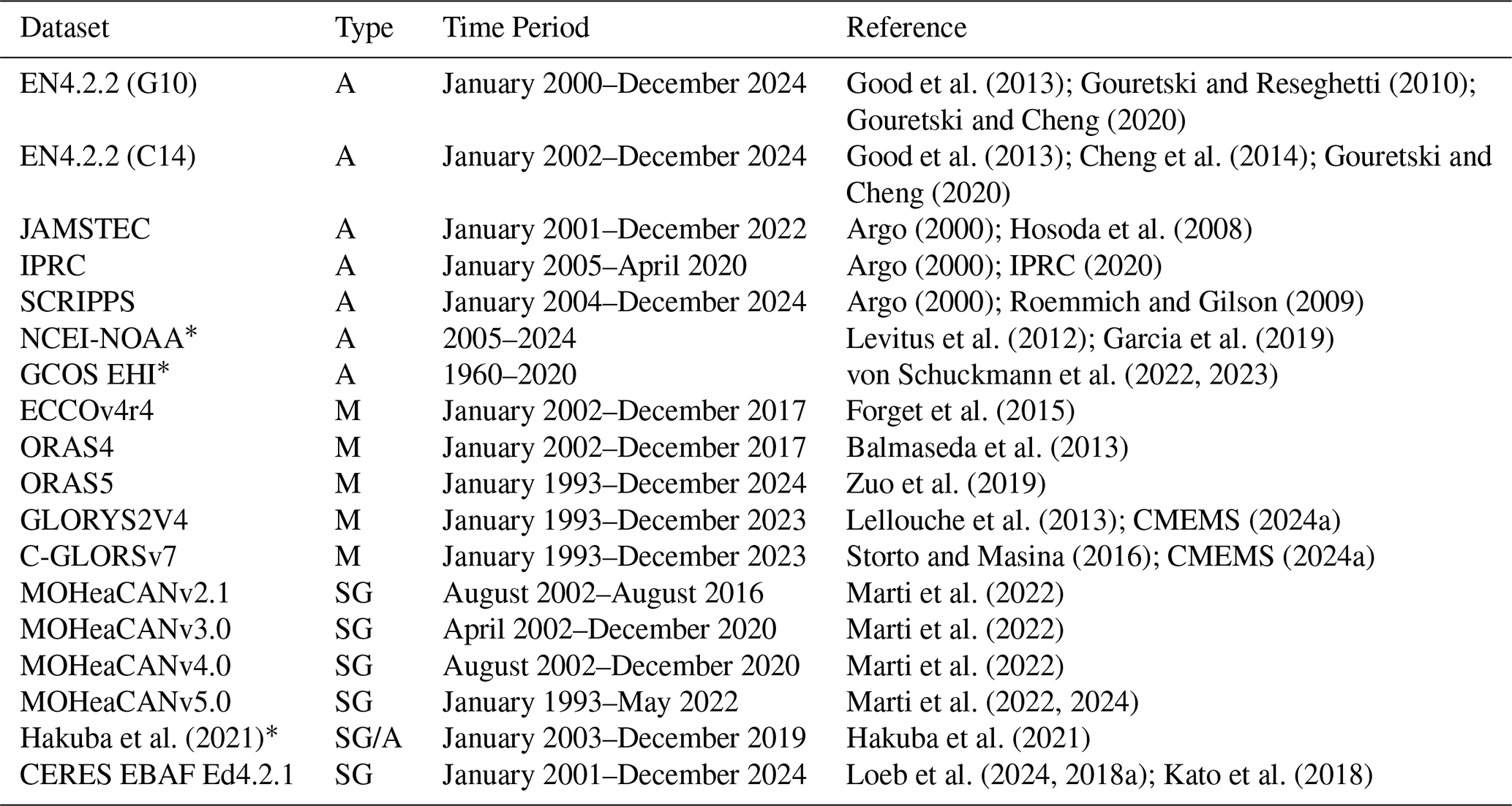
^* Data only available as global average.

Argo data were collected and made freely available by the International Argo Program and the national programs that contribute to it (https://argo.ucsd.edu, last access: 16 September 2026, https://www.ocean-ops.org, last access: 16 September 2026). The Argo Program is part of the Global Ocean Observing System. The Argo-only validation products are limited by the coverage of the Argo program and do not cover large parts of the polar oceans, which limits the validation in these regions (Fig. B1). In contrast, model products and the space geodetic data from MOHeaCAN are available for all ocean sub-regions investigated below. In order to better manage the number of datasets used here for validation and visualization, we computed ensemble means and corresponding spread for each of the three sub-categories. For this we also included prior MOHeaCAN versions 2.1, 3.0 and 4.0 (Table 1). All datasets provide data during the period January 2005 till December 2015, the “golden age” of ocean sampling (Palmer, 2017), which will be the basis for validation comparisons in the following.

3 Results

We investigate the quality of the OHC and OHU derived from various publicly available data products including model data, directly measured in situ temperature and salinity profiles from the Argo program and space geodetic approaches. The errors for each estimate are reported for the 95 % confidence (2σ) interval. In order to consider temporal correlations when analyzing the final time series, an auto-regressive process, similar to Rietbroek et al. (2016), has been assumed. Some of these datasets are only available as global time series, while gridded datasets can also be evaluated regionally. As all datasets cover different periods of time, we identified two analysis periods: (1) January 2005 till December 2015, which is covered by all datasets and allows for a direct comparison and (2) January 2005 till December 2024, which covers a span of 20 years, but is only provided by a hand full of published estimates.

3.1 The Sea Level Budget

Space geodetic approaches for computing ocean heat content (OHC) and it's rate, i.e. ocean heat uptake (OHU), generally require information on steric sea level change by computing a sea level budget. Here, we utilize a global fingerprint inversion method driven by satellite altimetry, satellite gravity and in situ profile data from the Argo program (Sect. 2.3). For the period January 2005 till December 2015, we find a global steric sea level rate of 1.24 ± 0.16 mm yr⁻¹, which together with a mass driven relative sea level change of 1.94 ± 0.16 mm yr⁻¹ closes the total sea level rise (3.18 ± 0.22 mm yr⁻¹) within a residual to observed altimetry sea level of 0.04 ± 0.08 mm yr⁻¹ (see Table A1 for the full budget). Note that while the mass, steric and total sea level changes are derived from gridded values covering the whole ocean with a resolution of 0.25°, the residual is computed directly at the 1 Hz along-track input altimetry data positions.

Total sea level from our inversion matches well with sea level estimated from using globally gridded monthly sea level (CMEMS, 2024b) of 3.15 mm yr⁻¹. If we evaluate total sea level change directly at the along-track altimetry locations our inversion estimate is found to be 3.41 mm yr⁻¹, which fits well to the 3.42 mm yr⁻¹ derived from sea level data based on Nerem et al. (2018). Similarly, inversion based mass sea level also corresponds well to independently processing the GRACE(-FO) data following Uebbing et al. (2019) resulting in 1.85 mm yr⁻¹. These sea level budget estimates, especially the steric sea level contribution, are in good agreement with published estimates (e.g., WCRP-Global-Sea-Level-Budget-Group, 2018; Horwath et al., 2022). With our inversion approach we can further split the steric contribution into a thermo- (1.22 ± 0.16 mm yr⁻¹) and halosteric (0.02 ± 0.02 mm yr⁻¹) components, where the former clearly dominates the estimate on global scales and is directly linked to OHC change, while the latter can have significant regional impact.

Regionally, we find good agreement between our trend maps for January 2005 till December 2015 (Fig. B2) and recent publications (Royston et al., 2020; Jeon et al., 2021). When comparing to results by Bouih et al. (2025) we find similarities between the patterns of total sea level change and Argo-based steric sea level and our results (Fig. B2), despite utilizing a slightly different time period for the derived trends. However, for the ocean mass change component Bouih et al. (2025) report significant trend anomalies in the North Atlantic ocean, also been mentioned by Mu et al. (2024), where the same region is also found to exhibit large residual trends, when subtracting the sum of all components from the total sea level observed by altimetry. From our fingerprint approach (Fig. B2C), we can not confirm these residual trend signals, similar to Jeon et al. (2021), who do not see these North Atlantic trend signals in the majority of their investigated products, including fingerprints, mascons and spherical harmonic solutions, except for the CSR spherical harmonic solution which shows slightly negative trends. EOF decomposition of our residual sea level (not shown here) reveals that there are no major trend signals left within our residual trends (Fig. B2G), as these are dominated by the major current regions (Gulf stream, Aghulas current, etc.), which are not modeled as part of our fingerprint approach. Similarly, we do not find significant positive residual trends in the Indian ocean as have been observed over the 2005–2015 period by others (Meyssignac et al., 2023, their supplement Fig. 5).

3.2 Global Ocean Heat Content Change

On global scales, we compare OHC from our GAAMR approach (Sect. 2.4) to OHC derived from various publicly available observational and model-based datasets (Sect. 2.6), as well as published estimates. In addition, one can directly compare to independently observed estimates derived from the CERES project. Monthly CERES EBAF-TOA Ed4.2.1 data (Loeb et al., 2018a, 2024) have been globally averaged in order to derive an estimate of EEI, which is then further converted to OHU and OHC.

On global scales, OHC change is mainly driven by seasonal changes as well as long term trends and accelerations (Fig. 1A). Considering CERES-OHC as independent reference, the seasonal signal from all other approaches generally agree well in phase, but show some larger amplitudes and variations in trend and acceleration. The latter becomes obvious after removing those aforementioned signals, computed over the reference period January 2005 till December 2015, from the individual datasets and comparing the residuals (Fig. 1B). During the computation period, the OHC estimates from different methods agree well, albeit being more noisy compared to the CERES-OHC. It becomes immediately clear that the variation in acceleration leads to significant disagreement, especially for the model ensemble after 2016. Estimates from our GAAMR method and based on converting inversion-derived steric sea level to OHC using a constant factor of 0.52 $\mathrm{W}{\mathrm{m}}^{-\mathrm{2}}(\mathrm{mm}{\mathrm{yr}}^{-\mathrm{1}}{)}^{-\mathrm{1}}$ agree quite well with the CERES-OHC also outside of the computation period after 2016; before 2005 we find also our estimates to be influenced by model deficiencies, likely stemming from non-global Argo data coverage being assimilated into the ORAS5 model, which is the basis for our steric fingerprints. In addition, inversion-based results (GAAMR and direct steric sea level conversions) show lower quality towards the end of the GRACE mission lifetime (after mid 2016), whereas results derived after the launch of the GRACE-FO mission in 2018 are again close to the CERES-OHC.

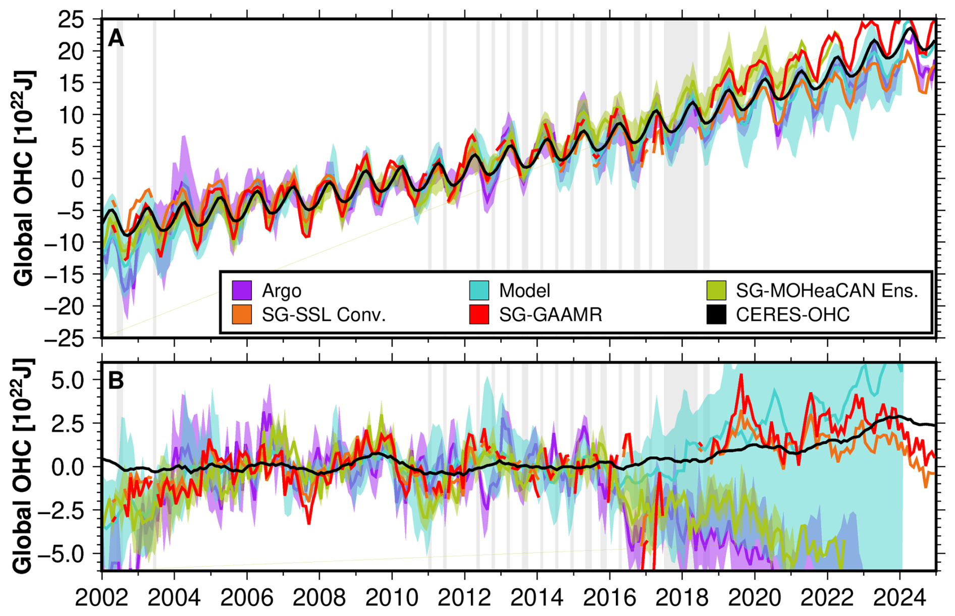
Figure 1 Global mean ocean heat content (OHC) change. (A) Full OHC signal. (B) Residual inter annual signal after removing the fitted signal (mean/trend/acceleration/seasonal) for the period January 2005 till December 2015. Months with missing GRACE/GRACE-FO data are indicated by the light-grey shaded vertical stripes. The groups Argo and Model are comprised by all corresponding data products from Table 1, whereas the space geodetic contributors consists of an ensemble of MOHeaCAN data (Table 1) and from our inversion results by directly converting steric sea level to OHC using a globally constant factor (Sect. 2.4.1) and our proposed GAAMR method (Sect. 2.4.2). The shading of the groups represents the full ensemble spread. Note: The residuals are computed over the aforementioned period and removed from the entire time series, leading to artifacts outside of the 11 yr period that is covered by all datasets. Outside of this analysis period and with fewer ensemble members residuals will become artificially large.

From our GAAMR method we find an overall increase of 1.34×10²² ± 0.12×10²² J yr⁻¹ for the period January 2005 till December 2015, which fits well into the range of OHC trend values reported by (Cheng et al., 2017; Resplandy et al., 2019; Cheng et al., 2022) based on several published estimates. When further separating OHC into contributions from the Northern and Southern hemispheres, we derive OHC rates of 0.52×10²² ± 0.11×10²² J yr⁻¹ and 0.82×10²² ± 0.14×10²² J yr⁻¹, respectively. The estimate for the Southern hemisphere compares well to Durack et al. (2018) and is in agreement with the findings reported in Intergovernmental Panel on Climate Change (IPCC) (2022). Our estimate for the Northern hemisphere is found to be slightly above the reported spread of results by Durack et al. (2018) but also in agreement with Intergovernmental Panel on Climate Change (IPCC) (2022).

Expressing the trends in OHC in terms of global OHU allows for further comparison between the individual datasets considered and our proposed GAAMR method (Fig. 2A, Table A2). We find OHU of 0.58 ± 0.14 W m⁻² from GAAMR with an OHU trend, i.e. OHC acceleration, of 0.20 ± 0.24 W m⁻² per decade (Fig. 2A, Table A2). While the OHU estimate shows the overall best agreement with that derived from the CERES project (0.67 W m⁻² per decade), the OHU trend derived from CERES is about double (0.41 W m⁻² per decade) what we find from GAAMR (Fig. 2B, Table A3). The difference in OHU trend likely results from a strong negative residual during 2007 and 2008 (Fig. 1B), which is driven by a significant scaling factor associated with the steric fingerprint representing the majority of the ENSO signal. While the CERES result does not seem to be strongly influenced by the La Niña event, similar negative residuals are found from the other datasets as well, albeit not as pronounced as in GAAMR (Fig. 1B). Considering all investigated datasets, we find a general spread of OHU between about 0.30–0.70 W m⁻² with some outliers exceeding these bounds (minimum: 0.08 ± 0.60 W m⁻² from A-SCRIPPS and maximum: 1.09 ± 0.12 W m⁻² from the ORAS5 reanalysis model). For the OHU trends, we find roughly 3 clusters of trend estimates (1) around 0.15–0.25 W m⁻² per decade (2) around 0.40 W m⁻² per decade and (3) around 0.55 W m⁻² per decade with some individual results exceeding these ranges up to 0.93 ± 1.04 W m⁻² per decade from A-SCRIPPS and even negative OHU trends (−0.26 ± 0.32 W m⁻² per decade and −0.39 ± 1.0 W m⁻² per decade for M-ORAS5 and M-Glorys2v4, respectively).

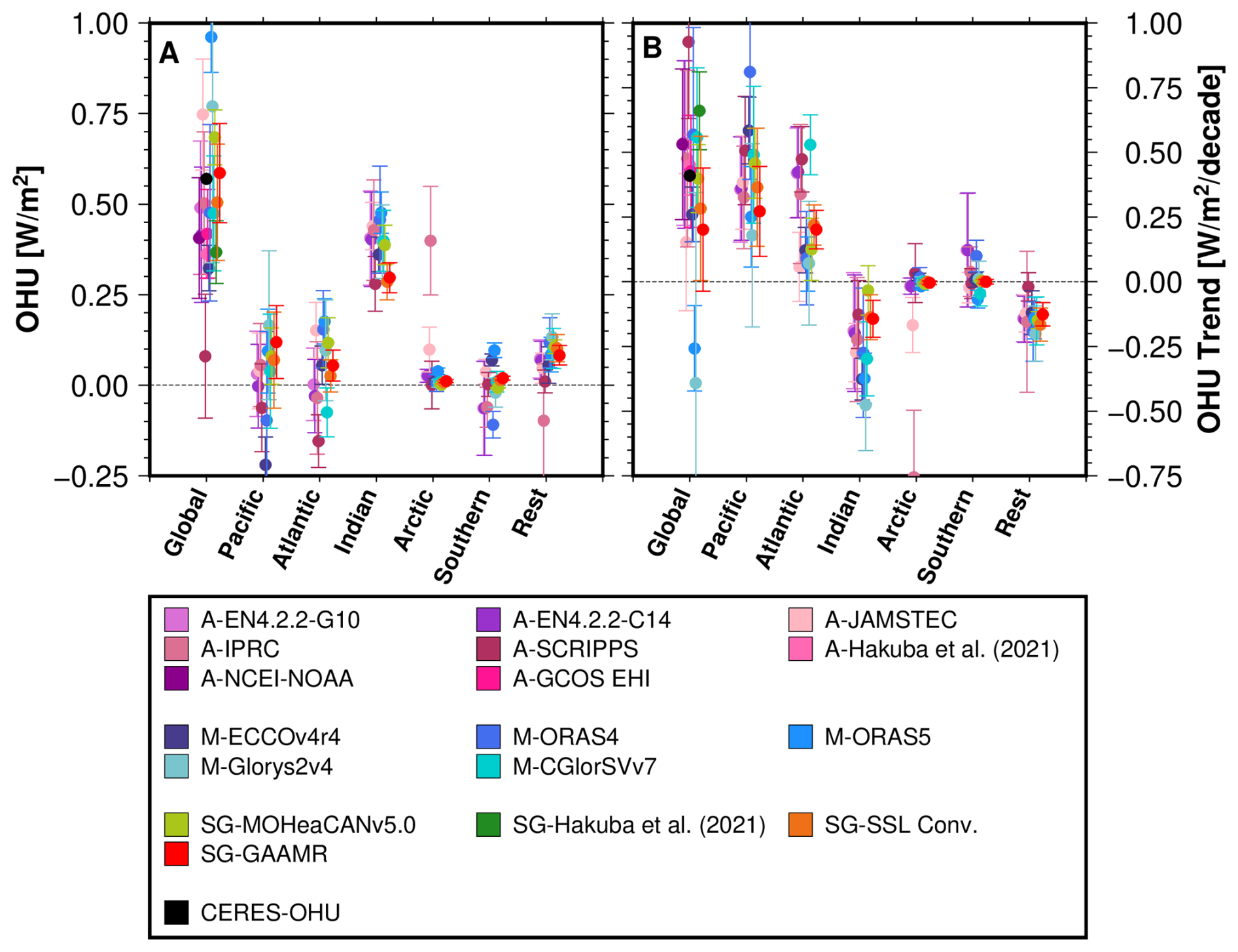
Figure 2 Ocean heat uptake (OHU) estimates (A) and corresponding OHU trends (B) derived from various Argo (A), model (M) and space geodetic (SG) datasets (Table 1) as well as our fingerprint inversion based GAAMR method (Sect. 2.4.2) for the period January 2005 till December 2015. Estimates are provided for the global ocean and individual sub-basins (see Fig. 3). Note that some datasets only provide global averages and can thus not be evaluated for the sub-basins.

Our estimated OHU fits well within the reported range of 0.53–0.74 W m⁻² by Meyssignac et al. (2019) for the period 2006 till 2015 extracted from in situ data, ocean reanalysis and converting steric sea level using a constant conversion factor. When we convert the reported ensemble mean (thermo-)steric sea level change of 1.31 ± 0.4 mm yr⁻¹ from for 2005–2015 (WCRP-Global-Sea-Level-Budget-Group, 2018) to 0.68 ± 0.21 W m⁻² using the constant factor 0.52 $\mathrm{W}{\mathrm{m}}^{-\mathrm{2}}(\mathrm{mm}{\mathrm{yr}}^{-\mathrm{1}}{)}^{-\mathrm{1}}$, the estimated OHU is higher than those estimated above. This can be explained by the constant factor not accounting for acceleration, which influences the estimated OHU. In other words, when directly converting the steric sea level trend to OHU, we find estimates more in line with considering only linear change as given in Table A4.

3.3 Regional Ocean Heat Content Change

On regional scales, comparison between individual datasets on ocean basin scales reveals significant differences (Fig. 3). Note that some datasets introduced in Sect. 2.6 are provided as global time series only and, thus, we include here only those datasets that can be evaluated in these sub-basins.

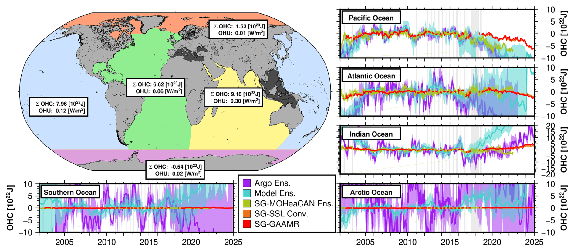
Figure 3 Regional ocean heat content change for the major ocean basins Atlantic, Pacific and Indian ocean, as well as the Arctic and Southern oceans, all defined according to internationally recognized boundaries (https://www.marineregions.org, last access: 16 September 2026). The remainder (simply denoted as “rest” in dark gray) consists of the Baltic Sea, Mediterranean and Black Sea and the Southeast Asian seas. Similar to Fig. 1B, residuals after removing mean, trend, acceleration and seasonal signal computed over the period January 2005 till December 2015 are show for each individual sub-basin. Note: The residuals are computed over the aforementioned period and removed from the entire time series, leading to artifacts outside of the 11-year period that is covered by all datasets. Outside of this analysis period and with fewer ensemble members residuals will become artificially large.

For the Pacific Ocean we find the residual curves from all datasets to agree relatively well during the analysis period with the space geodetic methods exhibiting a slightly lower noise level compared to the Argo and model-based ensembles (Fig. 3). Regarding OHU (Fig. 2A and Table A2), we find the Argo based methods on the lower end with estimates between −0.12 ± 0.16 W m⁻² and 0.06 ± 0.26 W m⁻². In contrast, the space geodetic approaches, including our GAAMR solution, provide slightly larger OHU estimates around 0.1 W m⁻², whereas the model-based estimates can differ significantly based on the model (−0.22 to 0.17 W m⁻²). Regarding OHU-trends, we find positive decadal trends from all datasets mostly concentrated in the range 0.25–0.50 W m⁻² per decade with some model based values exceeding these limits (Fig. 2B and Table A3). If we do not consider OHC accelerations, i.e. OHU trends, during estimation (Table A4), our OHU estimates for the Pacific Ocean are found to be larger compared to published Argo based estimates of 0.15 W m⁻² by Desbruyères et al. (2017). In contrast, it becomes significantly smaller when considering an OHU trend during estimation with only estimates from GAAMR (0.12 W m⁻²) and the Glorsys2v4 model (0.17 W m⁻²) showing good agreement.

For the Atlantic ocean, we find a generally higher spread and larger noise in the residual Argo and model ensembles compared to the Pacific ocean, while the space geodetic based residuals show a similar level around zero (Fig. 3). In terms of OHU, we find a similar level as for the Pacific ocean with our GAAMR estimate of 0.06 ± 0.04 W m⁻² located roughly in the middle of all individual estimates. Argo-based OHU is found to be smaller with most ensemble members even indicating negative OHU in the Atlantic, whereas space geodetic and all, but one, model OHU estimates are found to be positive (Fig. 2A and Table A2). For OHU trends we generally find significantly larger estimates for the Argo-based results above 0.3 W m⁻² per decade, while model estimates are found around 0.1 W m⁻² per decade (Fig. 2B and Table A3). Our GAAMR estimate (0.20 ± 0.08 W m⁻² per decade) lies between those two data groups. Similar to the Pacific Ocean, estimates for the Atlantic Ocean when not considering OHU trends (Table A4), are found to be roughly in line with the reported estimates around 0.17 W m⁻² by Desbruyères et al. (2017) and Rousseau et al. (2023), whereas estimates are systematically smaller in our normal processing, which considers OHU trends.

The residuals from the Indian Ocean (Fig. 3) show significant discrepancies between individual data groups. During the estimation period we, again, find space geodetic methods to exhibit the lowest noise level and relatively good agreement with model derived OHC residuals, while those from Argo are found to be noisier. In 2016, we find an artifact occurring for all Argo and all model data and to a much smaller extend also in the space geodetic data (Fig. 3). The reasons for this are currently unknown. Afterwards, a steep increase in OHC residuals can be observed from all model data, while Argo-based OHC-residuals increase at a significantly smaller rate. In contrast space geodetic results see no such significant increases in OHC residuals (Fig. 3). This data discrepancy is also reflected in the OHU estimates. On the one hand, we find a moderate OHU of 0.30 ± 0.04 W m⁻² from our GAAMR method, while most other datasets indicate stronger OHU estimates of 0.4–0.5 W m⁻² (Fig. 2A and Table A2). On the other hand, the same large OHU values are connected to strongly negative OHU trends of −0.40– −0.20 W m⁻² per decade, while we find only −0.14 ± 0.08 W m⁻² per decade from GAAMR and only −0.03 ± 0.10 W m⁻² per decade from the MOHeaCANv5 dataset (Fig. 2B and Table A3). Nonetheless, our estimates of Indian Ocean OHU significantly exceed the 0.17 W m⁻² reported in Desbruyères et al. (2017). If we do not consider an OHU trend during estimation, estimates are closer, albeit still slightly larger (Table A4).

While most datasets provide results in the Arctic and Southern oceans, for Argo datasets these are generally based on only a few grid cells as Argo provides only a very limited coverage of these high-latitude regions (see Fig. B1). This is also evident from the significant noise level in the OHC residuals for these two regions and a large ensemble spread after our analysis period (Fig. 3). Space geodetic and model estimates are less affected due to high latitude observation coverage and the model domains including these ocean regions. For the inversion, the fingerprint spatial patterns are assumed to be static over time, the global rescaling from the combined GRACE, altimetry and Argo observations nevertheless does provide “predicted” sea level change, budget and derived OHC from GAAMR in these high latitude regions. However, these still need to be interpreted with caution. While space geodetic missions show only very small residuals, model results show a larger noise level, albeit smaller as that found from Argo data. This is also reflected in the OHU and OHU trend estimates. For the GAAMR and MOHeaCAN space geodetic approaches we find OHU and OHU trends close to zero, while model estimates, especially for the Southern Ocean, can reach values of up to ±0.1 W m⁻² (Fig. 2A and Table A2) and an OHU trend range of −0.07–0.1 W m⁻² per decade (Fig. 2B and Table A3). While we report the estimated Argo values, we do not consider those representative considering the very limited Argo coverage in these regions and the significantly different number of provided grid cells from each Argo product. Desbruyères et al. (2017) report a very large contribution of 0.24 W m⁻² based on Argo for the Southern Ocean, which we cannot confirm here.

Despite covering only 3 % of the ocean area, the contribution of the remaining ocean, which includes warming of e.g., the Mediterranean Sea, the Baltic Sea and the Asian Seas, including the Indonesian Throughflow, is found at levels of to 10 % of the global OHU. We find a general good agreement between OHU and OHU trend estimates from all products with our GAAMR results fairly in the middle with a contribution of about 0.1 W m⁻² OHU and −0.15 W m⁻² per decade OHU trend (Fig. 2 and Tables A2 and A3). Most of these regions represent shallow seas where sea level changes are dominated by water mass changes and transports resulting from remote steric effects. For the Southeast Asian seas this remote steric effect in combination with steric variability in non-shallow regions, such as the South China Sea (e.g., Xi et al., 2019) drive the majority of the OHU. In other words, the heat in this region rather acts as a compensation for missing signal outside of these regions. Furthermore In addition, local thermo- and halo-steric effects in the Mediterranean Sea (Carillo et al., 2012; Margirier et al., 2020) also contribute on a smaller scale.

3.4 Twenty Years of Space-Geodetic Ocean Heat Content Change

In the following we present results for an extended data period, i.e. January 2005 till December 2024. However, not all of the data products are available until end of 2024 and thus, we limit our presented results to three Argo products, one model result, as well as our own computations based on converting steric sea level directly and our GAAMR approach.

The global OHC residuals, after removing mean, trend, acceleration and seasonal signals, (Fig. 4A), show a good agreement between independent data from the CERES project and our space geodetic results, similar to the above analysis period. This is also reflected in the OHU (Fig. 4B and Table A5), where we find 0.57 W m⁻² and 0.61 ± 0.10 W m⁻² from the CERES project and GAAMR, respectively. While OHU estimates from Argo also agree within error bounds, that from the ORAS5 model is significantly larger (0.82 ± 0.12 W m⁻²). Global trends in OHU (Fig. 4C and Table A6) derived from the CERES project are found to be almost double of what has been found from the other data products (0.41 W m⁻² per decade). Argo and model OHU trends are found generally smaller compared to that from GAAMR, which appears to be mainly driven by OHU trend differences in the Pacific and Indian oceans (Fig. 4C and Table A6).

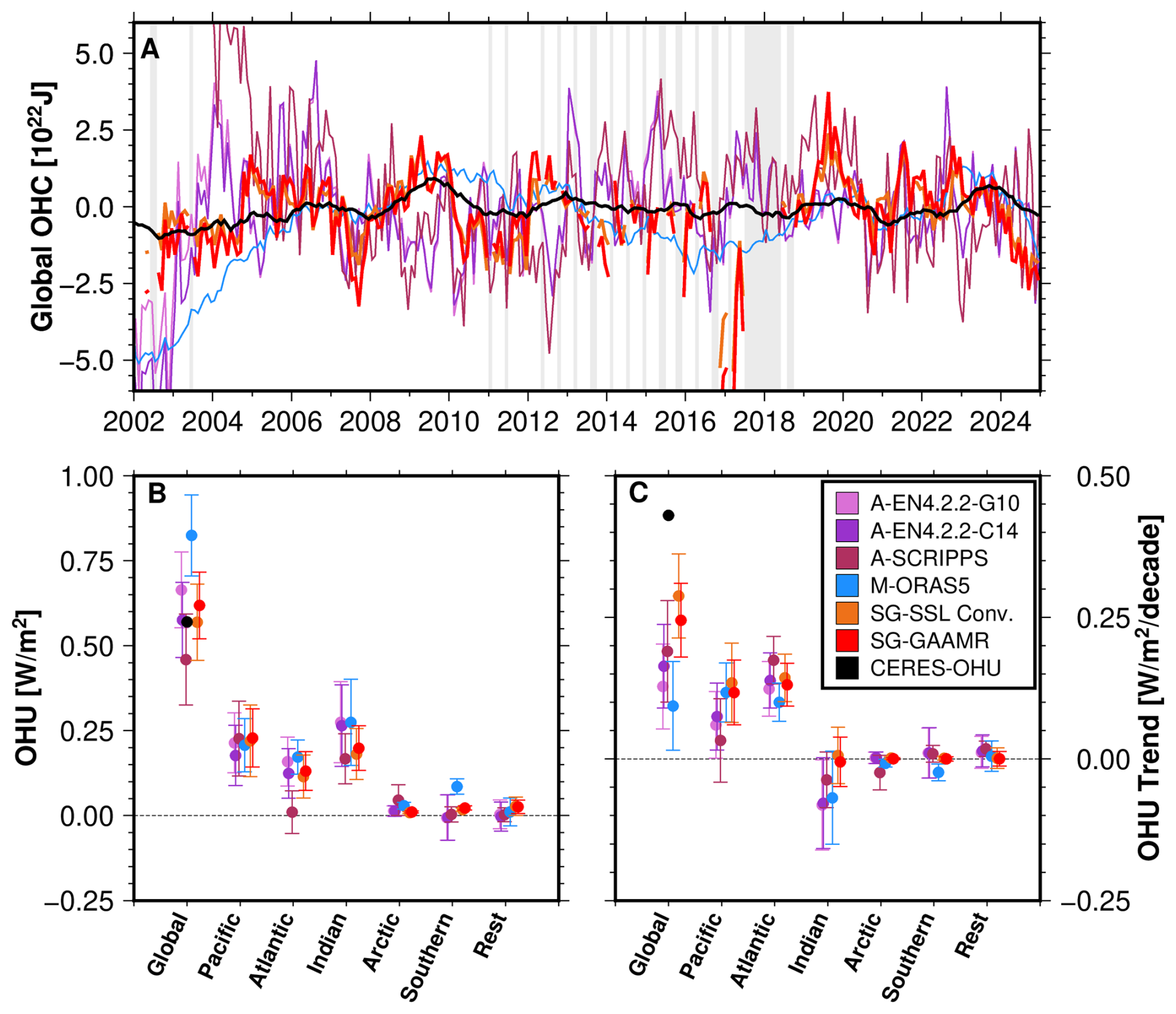
Figure 4 OHC and OHU results over 20 years for the time period January 2005 till December 2024 for individual Argo (A), model (M) and space geodetic (SG) data products. (A) Residual inter annual ocean heat content (OHC) signal after removing the fitted signal (mean/trend/acceleration/seasonal) for the period January 2003 till December 2024. Months with missing GRACE/GRACE-FO data are indicated by the light-grey shaded vertical stripes. (B) Ocean heat uptake (OHU) comparison on global and regional scales. OHU trend comparison on global and regional scales.

Regional OHU over the extended period in the Pacific and Atlantic oceans is found to be similar to the analysis period (2005 till 2015) reported above (Fig. 2) around 0.1 W m⁻² for both with all estimates agreeing within error bounds. Only the Argo solution from SCRIPPS shows a significantly smaller OHU. In contrast, estimates for the Indian ocean are found to be significantly smaller (0.2–0.25 W m⁻²) over the extended estimation period (Fig. 4B) compared to the shorter period (Fig. 2A). At the same time corresponding trends in OHU, which have been negative for the shorter period (Fig. 2B) are found to be closer to zero (Fig. 4C). Similar to the shorter analysis period, we find OHU and OHU trend values close to zero for the Artic and Antarctic oceans. OHU from the remaining part of the ocean is also found to be close to zero, whereas it accounted for about 0.1 W m⁻² for the shorter analysis period.

We compare the spatial patterns of OHU (Fig. 5) and OHU trends (Fig. 6) on grid level. We generally find good agreement with respect to the distribution of larger regions of positive and negative OHU (and OHU trends). OHU from ORAS5 is generally very similar to that from converting steric sea level using a temporally constant factor and our GAAMR method due to ORAS5 representing the basis for our steric fingerprints used within the inversion approach. However, spatial patterns are not identical, but rather differ in details, e.g. in the northern and equatorial Atlantic ocean, the central Indian ocean or the Southern ocean (Figs. 5 and 6). We find negative OHU in the northern Atlantic, which have been linked to a weakening of the Atlantic meridional overturning circulation (Rahmstorf et al., 2015), where a collapse would significantly increase ocean warming (Nian et al., 2026). In contrast, the patterns derived from EN4 appear more generalized with less detail, which is mainly due to the lower grid resolution compared to the other results (1.0 vs. 0.25°). Furthermore, this results from the covariance lengths used in the objective analysis which have length of 300–400 km at the equator, which can be increased exponentially to 1500 km towards the poles (Good et al., 2013). In addition, we find differences in OHU and corresponding trends in the northern Atlantic and the southern Pacific oceans, as well as around southern Australia, where the Argo data suggests significant positive OHU, while model and space geodetic results point to a region of significant negative OHU. While the global oceans are mostly warming (Johnson and Lyman, 2020), there has also been regional cooling, e.g., in the (sub-)tropical Pacific (Fig. 5), which have been linked to a general “La Niña-like” strengthening of the zonal ocean heat gradients (Lee et al., 2022). Changes in the Indian Ocean Walker circulation leading to a general warming in the Arabian Sea (Sharma et al., 2023) and the northern part of the Indian Ocean. These transports from the Indian Ocean equatorial region have been linked to El Niño-Southern Oscillation and Indian Ocean Dipole signals in the past (Sreenivas et al., 2012).

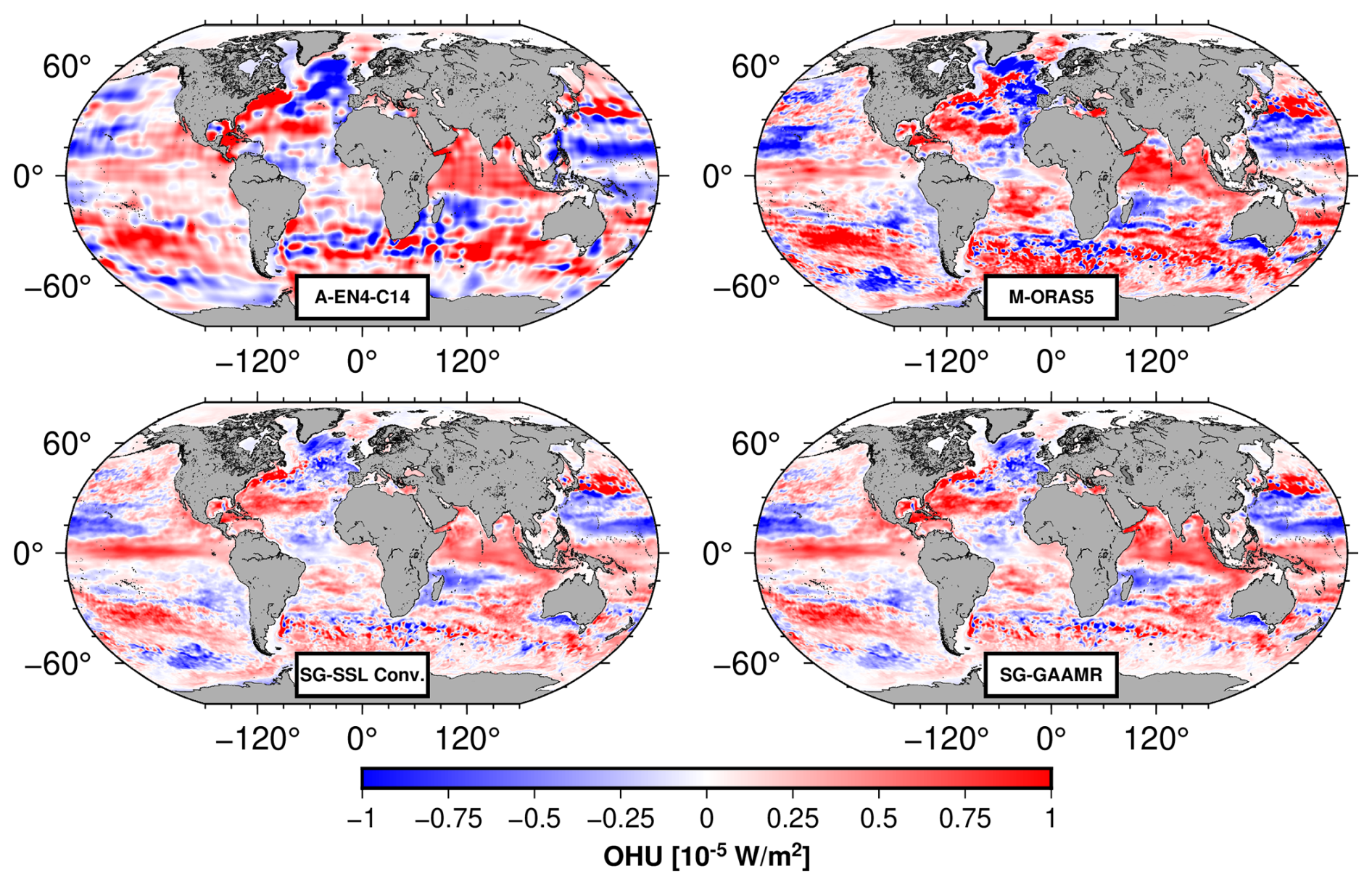
Figure 5 Regional ocean heat uptake (OHU) over January 2005 till December 2024.

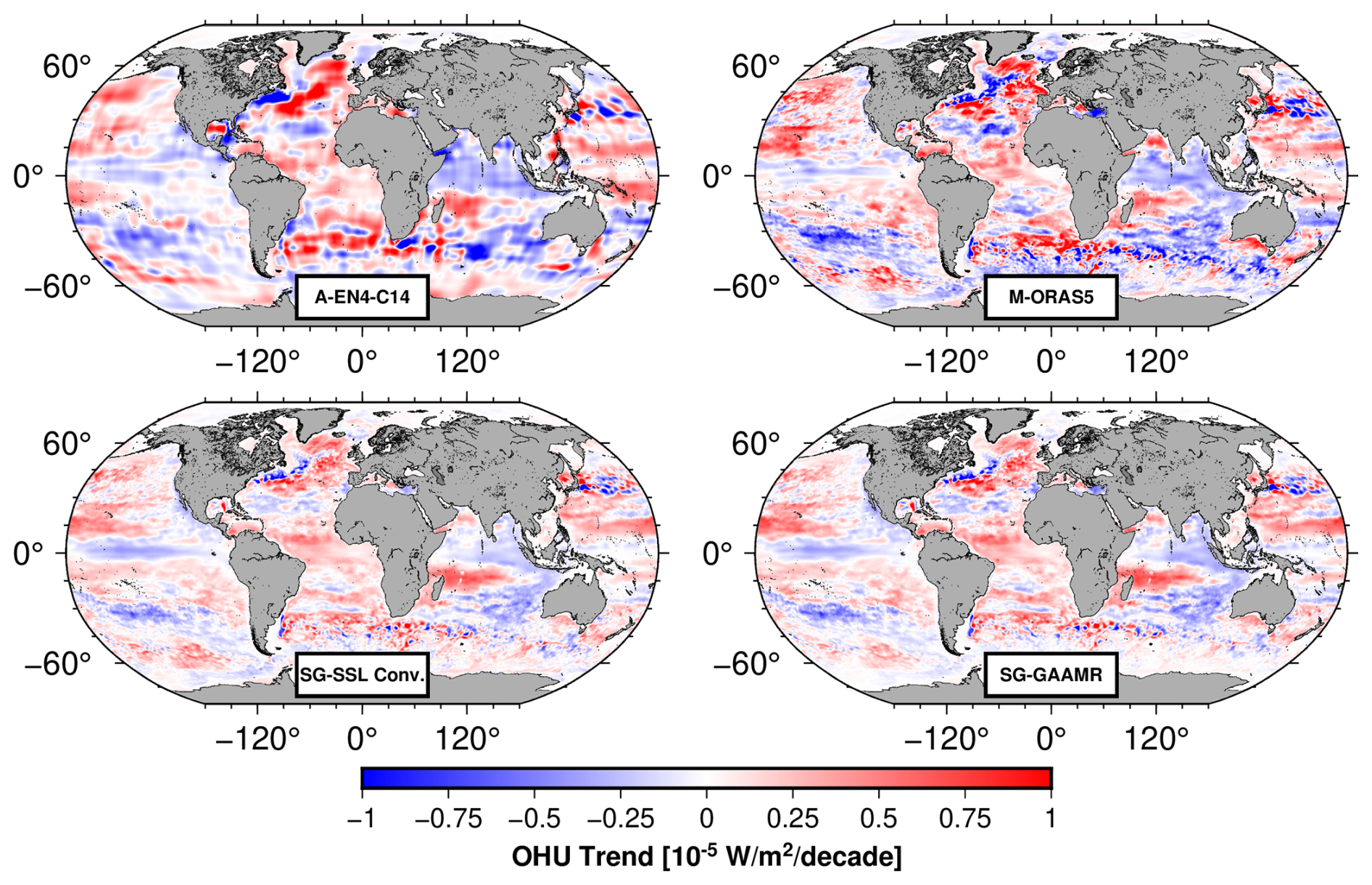
Figure 6 Regional ocean heat uptake (OHU) trend over January 2005 till December 2024.

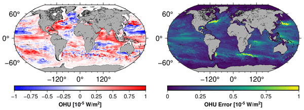
By propagating the formal errors of thermosteric sea level from our inversion output throughout our GAAMR method and also assuming a 5 % ORAS5 reanalysis error level during conversion to OHC, regional errors of OHU and OHU trends are shown in Fig. 7. These represent the errors corresponding to the GAAMR results in Figs. 5 and 6. Largest errors are detected in major current regions, including the Gulf steam, the Aghulas current and the Kuroshio current. This is expected as thermosteric variability in these regions is large due to eddy and gyre presence.

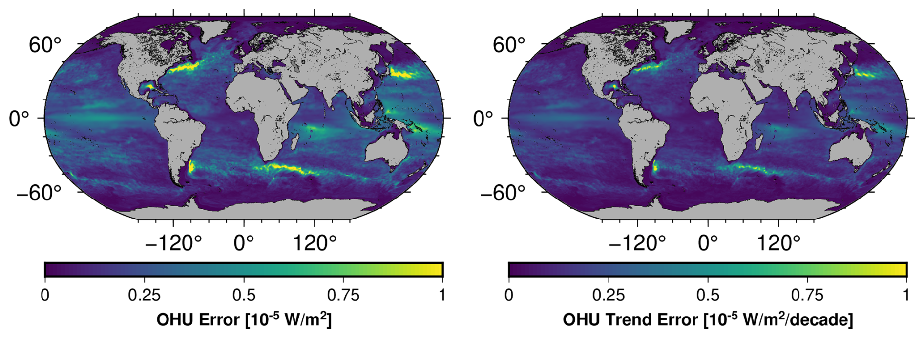
Figure 7 Regional ocean heat uptake (OHU) errors and OHU trend errors as derived from our GAAMR method over January 2005 till December 2024.

The Hovmöller diagram in Fig. 8 shows the inter-annual spatial ocean heat distribution for the major ocean basins of the Pacific, Atlantic and Indian Oceans, derived from GAAMR and ORAS5, with sea surface temperature (SST) from the ERA5 reanalysis for comparison (Copernicus Climate Change Service, 2023). For computing the inter-annual signal, we remove the monthly climatology (January 2005 till December 2024) as well as the OHC trend and acceleration signal (Figs. 5 and 6). Generally, we find the GAAMR signal to be lower compared to the ORAS5 reanalysis, similar to our results on regional OHC reported above.

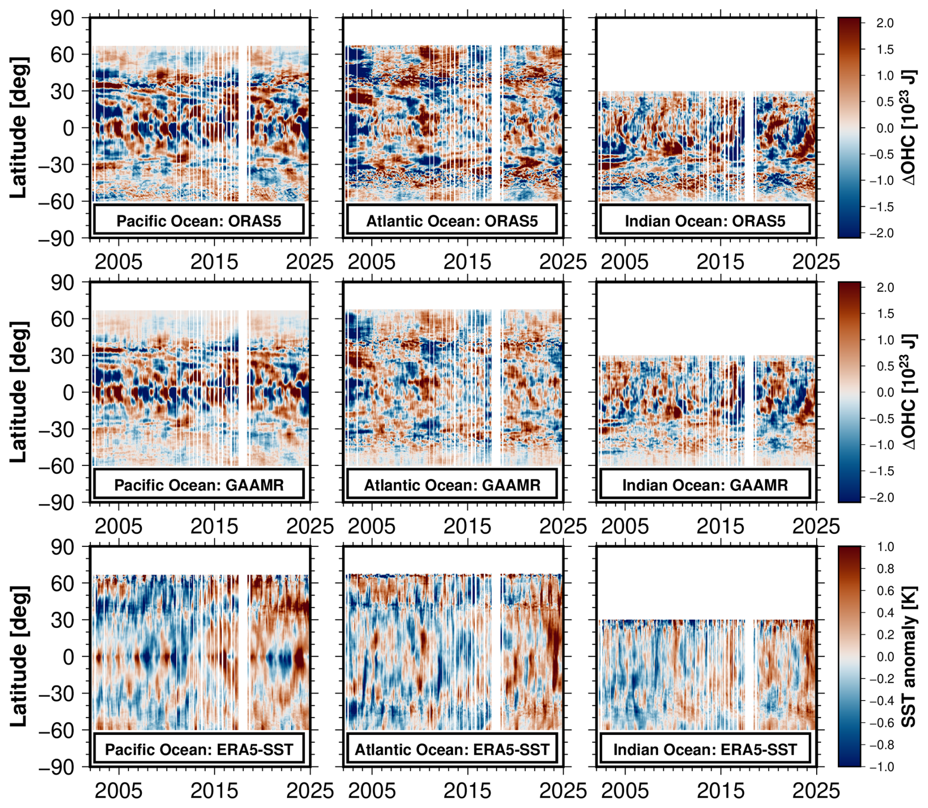
Figure 8 Spatial residual ocean heat content (OHC) distribution in the major ocean basins of the Pacific, Atlantic and Indian Oceans from our GAAMR method, ORAS5 reanalysis data in comparison to sea surface temperature (SST) (Copernicus Climate Change Service, 2023). All datasets have their climatology, computed over January 2005 till December 2024 as well as their respective trend signal removed and are averaged over all longitudes within the respective ocean basin. Due to lack of GRACE(-FO) data some months of are missing from our GAAMR results and have also been removed from the ORAS5 and SST reanalysis datasets for visual consistency.

At inter-annual timescales in the equatorial Pacific Ocean, we observe alternating patterns of warming and cooling that correspond to the ENSO signal (Fig. 9). From the GAAMR results, transport of ocean heat is observed in the tropical and sub-tropical Pacific Ocean (Fig. 8). Warm water is concentrated around 30° N until about 2005 and then slowly propagates southward toward the equator until about 2010. Afterwards, warm water is propagating northward again until about 2014. After 2014, a relatively large warming region is observed in the sub-tropic zone. A similar but less pronounced transport is found in the tropical zone of the Southern hemisphere. These transport periods align well with the Pacific Decadal Oscillation (PDO, Fig. 9), which has been found to be linked to variability in EEI at the top of atmosphere (Loeb et al., 2018b, 2021). Towards the polar regions, we generally find decreasing OHC, which is different to SST. SST clearly also shows effects from the marine heat wave “blob” (Bond et al., 2015; Chen et al., 2023). Indeed we find the same pattern, albeit much less pronounced, also in whole-water-column OHC from GAAMR (Fig. 8).

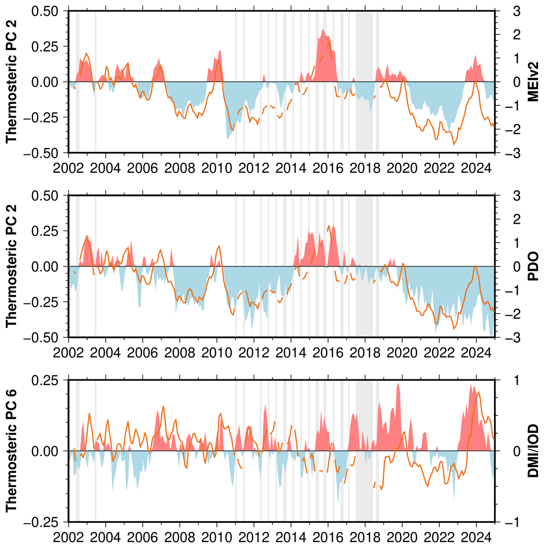
Figure 9 Comparison between individual principal components (PC, orange lines) involved in the GAAMR method to major climate indices (red/blue shaded), including the Multivariate ENSO Index (MEIv2, Kobayashi et al., 2015), the Pacific Decadal Oscillation (PDO, Newman et al., 2016) and the Indian Ocean Dipole (IOD, Saji and Yamagata, 2003).

Differences in the details of the inter-annual spatio-temporal signal structure are observed between GAAMR and ORAS5, e.g. in the (sub-)tropical southern part of the Atlantic in 2011 and 2012 (Fig. 8). This again highlights the ability of GAAMR to adapt not only to variations in amplitude, but also spatial signal variations. We observe a clear signal in SST between 30 and 40° N, which is, albeit significantly less pronounced, visible also in OHC distribution from GAAMR as well as ORAS5. From GAAMR we observe reduced heat variability in the tropical zone and even after the large ENSO event in 2010 the corresponding heating over the entire water column is less pronounced and slightly lagging behind the SST signal.

In the Indian Ocean, we find the inter-annual signals in the northern part and the tropical zone exhibiting a distinctive pattern of North-South stripes in the SST spatial distribution (Fig. 8), which can be linked to ENSO periods (Fig. 9). Here, we find a more lagged response with warm and cold water being transported northward driven by a change in the Indian Ocean Walker circulation leading to a general warming in the Arabian Sea (Sharma et al., 2023). These transports from the Indian Ocean equatorial region have been linked to ENSO and Indian Ocean Dipole (IOD, Fig. 9) signals in the past (Sreenivas et al., 2012). After 2018, we find generally larger levels of heat transport from the equatorial Indian ocean towards the North and, to a smaller extent, to the South. This indicates an explanation for the lower OHU levels observed for the 20 year period compared to the shorter analysis period (Figs. 2 and 4).

We finally investigate the connection between our GAAMR results and well defined major climate indices (Fig. 9). We find strong correlation of 0.82 between the principal component of the second mode of the GAAMR approach and the Multivariate ENSO Index (MEIv2, Kobayashi et al., 2015) index. Similarly, the PC of the second mode is also closely linked to the Pacific Decadal Oscillation (PDO, Newman et al., 2016) index, where we find a correlation of 0.71. Thus, the second mode within GAAMR represents, both, the ENSO variability and the PDO variability, e.g. following the general trend into the negative seen in PDO after 2016 while having the MEI variability superimposed. Our correlation results are in line with those reported by Loeb et al. (2021) who compared sea surface temperature (SST) anomalies to indices for ENSO and PDO, which has been linked to variability in EEI before (Loeb et al., 2018b). Other indices, such as the Indian Ocean Dipole (IOD, Saji and Yamagata, 2003) index, can not be directly linked to a single mode in GAAMR, but are rather spread over multiple modes. In order to achieve a clear signal separation for these weaker signals from EOF decomposition, one would need more data, i.e. a significantly longer time series.

4 Discussion

Published estimates of OHU, especially those derived from satellite altimetry and GRACE gravimetry, generally focus on global OHU and its relation to EEI. In fact, regional OHC is usually analyzed based on model data or in situ Argo profiles (e.g., Desbruyères et al., 2017) or focusing only on individual ocean basins, such as the Atlantic Ocean (e.g., Rousseau et al., 2023). Only few regional satellite geodetic OHC products exist (e.g. Marti et al., 2022). Our results have revealed significant discrepancies between GAAMR, i.e. satellite-observed OHU, and estimates directly derived from in situ Argo profiles (e.g., Desbruyères et al., 2017). We believe this is unequivocally connected to the difference in spatial coverage between Argo and satellite data. While satellite altimetry and GRACE gravimetry provide global coverage with regular observation time steps, availability of in situ Argo profiles is driven by the ocean currents resulting in regions of high spatio-temporal coverage and those with only scarce to none measured profiles (Fig. B3). With the GAAMR approach, it is possible to derive satellite observation driven global and consistently processed regional OHC, OHU and OHU trends.

For the period January 2005 till December 2015 we find the global OHU to be dominated by the Indian Ocean heat storage, while also showing a strong negative trend. At the same time, the “rest” ocean contributes to global OHU on similar levels as the Atlantic and Pacific oceans. These large OHU of the Indian Ocean has been attributed to excessive heating of the Pacific Ocean during the warming hiatus, which in turn led to increased heat transport into the Indian Ocean through the Indonesian throughflow (Lee et al., 2015). The latter also explains the stronger OHU signal in the “rest” component in our analysis as this contains the Indonesian throughflow. For the longer analysis period (January 2005 till December 2024) the Indian ocean contribution to global OHU is found to be almost half compared to the shorter period and roughly on par with the Pacific Ocean contribution. Since the “rest” contribution is close to zero over the longer time period this likely indicates that the heat transport in the Indonesian throughflow over the longer analysis period cancels out. This indicates a transformation towards a more evenly distributed global heat budget over the longer period. In addition, the shorter time period covers only 11 years, which may be fine for a general comparison for the individual data products, but regarding estimating robust and meaningful long-term OHU and OHU trends a longer time period of 20+ years is preferable (Intergovernmental Panel on Climate Change (IPCC), 2014).

Other studies find significantly larger contributions from the Southern Ocean (e.g., Li et al., 2023). Generally this results from a different definition of the discussed ocean regions. The northern boundary is often defined to be around 30 to 40° S, while we utilize internationally recognized boundaries (https://www.marineregions.org, 16 September 2026), which cut off the Pacific, Atlantic and Indian Ocean basins at 60° S. Significant portion of ocean warming is found between 30 to 60° S, which we attribute to the respective ocean basins instead of the Southern Ocean.

We also found larger estimates of global OHU from the ORAS5 and Glorsys2v4 model reanalysis as well as SCRIPPS derived in situ OHC (Fig. 2A and Table A2), in contrast to most other datasets. This seems to be mostly driven by significant OHU in the Indian Ocean, which might point to some modeling issues in this region. Our GAAMR approach did not show these extreme values in the Indian Ocean region, despite utilizing the modes derived from ORAS5 steric sea level within the inversion. Of course, differences in regional sea level budget modeling may also affect OHU results. As shown above, Meyssignac et al. (2023) found large residual trends in the Indian ocean, while our inversion results (Fig. B2G) show significantly smaller trend levels and smaller scale features. We believe this inspires confidence in the fingerprint-based results. While the spatial pattern might be pre-defined by the model data, this also shows that the inversion result and, thus, GAAMR is adapted to the observed data and not strictly controlled by the underlying model.

Our results showed artifacts in global and regional OHC residuals before 2005 (Figs. 1 and 3), which we believe to be likely related to assimilation artifacts from spatio-temporal heterogeneous Argo coverage (Zuo et al., 2019). In addition, spurious drifts in Argo conductivity sensors observing salinity after 2016 impact Argo, based estimates of steric sea level change and ocean heat content (Wong et al., 2020; Barnoud et al., 2021), and therefore to some extent the model reanalyses, which also assimilate in situ temperature and salinity profiles. Similar effects are also observed for the global ocean as well as other ocean basins affecting trends and seasonal signals. GAAMR can be viewed as correcting such drifts by utilizing the inversion estimates based on GRACE and altimetry in conjunction with in situ Argo observations.

CERES-based estimates of OHU require assumptions about heat uptake by other parts of the Earth system, which store heat, such as the land, ice or atmosphere. In this study, we have adopted a value of 90 % (von Schuckmann et al., 2020) of the Earth excess heat being stored in the oceans. When adopting 93 % as in (e.g., Trenberth et al., 2016) we find changes in OHU of less than 0.05 W m⁻². In addition, there is the caveat that the CERES EBAF dataset, that is commonly employed for deriving EEI, is already corrected for instrument biases by adjusting the original (SYN dataset) EEI to precomputed values of land, ice, atmosphere and ocean based heat uptakes (Loeb et al., 2018a), which is an inherent source of potential biases and errors during validation. This means the dataset is not entirely independent from other estimates. As such it can only be used for comparison of results, but does not serve as a completely independent reference. In addition, CERES-based OHU trends for the 2005–2025 analysis period are found to be significantly larger compared to other estimates (Fig. 4). Since the OHU trend value is basically the same as in the shorter period (2005–2015) this might either point to heat being increasingly stored in other parts of the Earth's system or an issue with the bias adjustment when deriving the CERES EBAF data.

Inferring OHC change or OHU utilizing a constant conversion factor of 0.52 $\mathrm{W}{\mathrm{m}}^{-\mathrm{2}}(\mathrm{mm}{\mathrm{yr}}^{-\mathrm{1}}{)}^{-\mathrm{1}}$ on global average (e.g., Meyssignac et al., 2019; von Schuckmann et al., 2020; Hakuba et al., 2021) is a convenient approach for converting steric sea level change obtained by subtracting GRACE(-FO) observed ocean mass change from altimetry measured total sea level variations. On global scales this method yields decent results, but generally provides slightly smaller estimates compared to the CERES reference as evident in Fig. 2A from the Hakuba et al. (2021) estimate and the SSL Conv. result directly converting our inversion based steric sea level to OHU using the aforementioned factor. In fact, the conversion factor is not constant but varies on spatial scales (Fig. B4) as well as, to a very small extent, temporal scales.

Utilizing the individually computed altimetry based (CMEMS, 2024b) and GRACE(-FO) ocean mass change (Uebbing et al., 2019) time series mentioned earlier one can easily derive steric sea level change and from that a corresponding OHU of 0.49 W m⁻², which corresponds well to that derived from converting steric sea level from our inversion (SSL Conv.). However, steric sea level derived this way includes thermo- as well as halosteric components. On global scales the halosteric part may be negligible, but it can have significant impact regionally, which makes approaches simply applying the global conversion strategy to regional steric sea level results susceptible to halosteric impacts.

In contrast, our inversion approach is able to separate thermo- and halo-steric sea level components by utilizing in situ Argo data in conjunction with the GRACE(-FO) and altimetry observations in a consistent joint framework. Furthermore, GAAMR extends the conventional approach of scaling with only one constant factor to instead splitting the scaling process into individual modes and scaling those independently. This allows to account for spatial and temporal variations based on the utilized fingerprints and the corresponding scaling factors. The good agreement of these thermosteric changes converted to OHU, utilizing the GAAMR processing, to data from the CERES project lead us to believe our approach to be beneficial, especially on regional scales.

Major current regions, such as the Gulf stream, Agulhas or Kuroshio current, are found to exhibit the largest uncertainties in OHU. These are expected to a certain extent as these regions also exhibit the largest residual signals (Fig. B2G), as the highly temporally variable currents and eddy regimes are not well modeled by the static fingerprint approach. Besides propagating the measurement errors of the input datasets itself, combination of inconsistent signals may add to the uncertainties due to differences in corrections applied to individual datasets. However, we preprocessed all input datasets to be as consistent as possible in terms of applied corrections, e.g. utilizing the same GIA model for correcting GRACE(-FO) and satellite altimetry. A third part of the uncertainty budget, which is difficult to quantify, directly relates to the fingerprints employed in our approach, as limited representativeness of the fingerprints directly influences the separation of the total sea level into mass and steric components, which in turn translates to a direct influence on our GAAMR results. Finally, the involved model data, in this case ORAS5, does not provide error information and we simply assume a 5 % model error during error propagation within the GAAMR processing. In summary this means that our GAAMR results, while showing good agreement with other datasets, are still affected by different error sources, where some have reduced impact due to meticulous processing.

5 Data availability

Monthly gridded OHC data from our Grace, Altimetry and Argo Mode Rescaling (GAAMR) method together with corresponding error estimates is available from https://doi.org/10.1594/PANGAEA.994058 (Uebbing and Kusche, 2026).

6 Conclusions

We introduced the GRACE, Argo and Altimetry based Mode Rescaling (GAAMR) method, representing an extension to our global fingerprint inversion approach, which allows to separate individual mass and steric sea level components by combining GRACE(-FO) gravity, satellite altimetry and in situ Argo profile datasets consistently within a joint estimation framework. For the period January 2005 till December 2024 we find global OHU of 0.62 W m⁻², which agrees well with a variety of published datasets from in situ Argo data, model reanalyses and space-geodetic approaches as well as independent estimates from the CERES project. By leveraging the information from the rescaled modes of OHC from our GAAMR approach, we find the global OHU to be driven mainly by warming of the Pacific Ocean (0.23 W m⁻²), followed by contributions from the Indian (0.20 W m⁻²) and Atlantic (0.13 W m⁻²) oceans. Small contributions are found from the Arctic Ocean (0.01 W m⁻²), the Southern Ocean (0.02 W m⁻²) and the remaining ocean (0.03 W m⁻²). We suggest that GAAMR results provide more robust estimates of an increasing OHU as compared to ocean reanalyses or the conventional single-scaling factor approach. The latter requires a single constant conversion factor, where often simply the global average is utilized. While this works sufficiently well on global scales, regionally OHC exhibits spatio-temporal variations, which can not be mapped by a constant factor. With GAAMR, we utilize the fingerprint basis from our sea level budget inversion and perform a mode-based conversion of thermosteric sea level to OHC, while preserving space-geodetic observation based temporal variations for each individual mode. This leads to more robust estimates, especially on regional scales.

However, our GAAMR method is limited by the availability of various datasets, most and foremost the input GRACE(-FO) gravity data in order to separate mass and steric sea level. Gaps in this dataset can occur and no GAAMR results are provided during missing GRACE(-FO) month. Consequently, expansion of the time series by filling the gaps between missing GRACE month and especially between GRACE and its successor GRACE-FO, e.g. by incorporating time-variable gravity from the Swarm mission (Lück et al., 2018), will enable derivation of a continuous observation driven time series of OHC and improve global and regional OHU.

Appendix A: Tables

Table A1 Sea level budget derived from fitting GRACE(-FO), satellite altimetry and in situ Argo data consistently within a joint fingerprint inversion framework. Note that the residual component has been computed at the along-track input altimetry positions. Errors are provided as one sigma values.

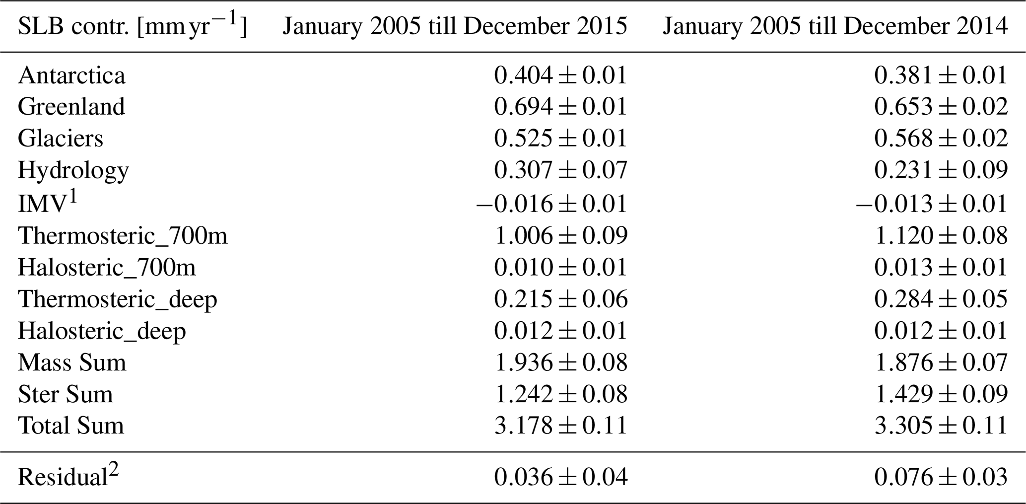
¹ Internal Mass Variations. ² Evaluated at input altimetry positions.

Table A2 Comparison of ocean heat uptake (OHU) from individual Argo (A), model/reanalysis (M) and space geodetic (SG) data sources. Analysis period: January 2005 till December 2015. Errors are provided as one sigma values.

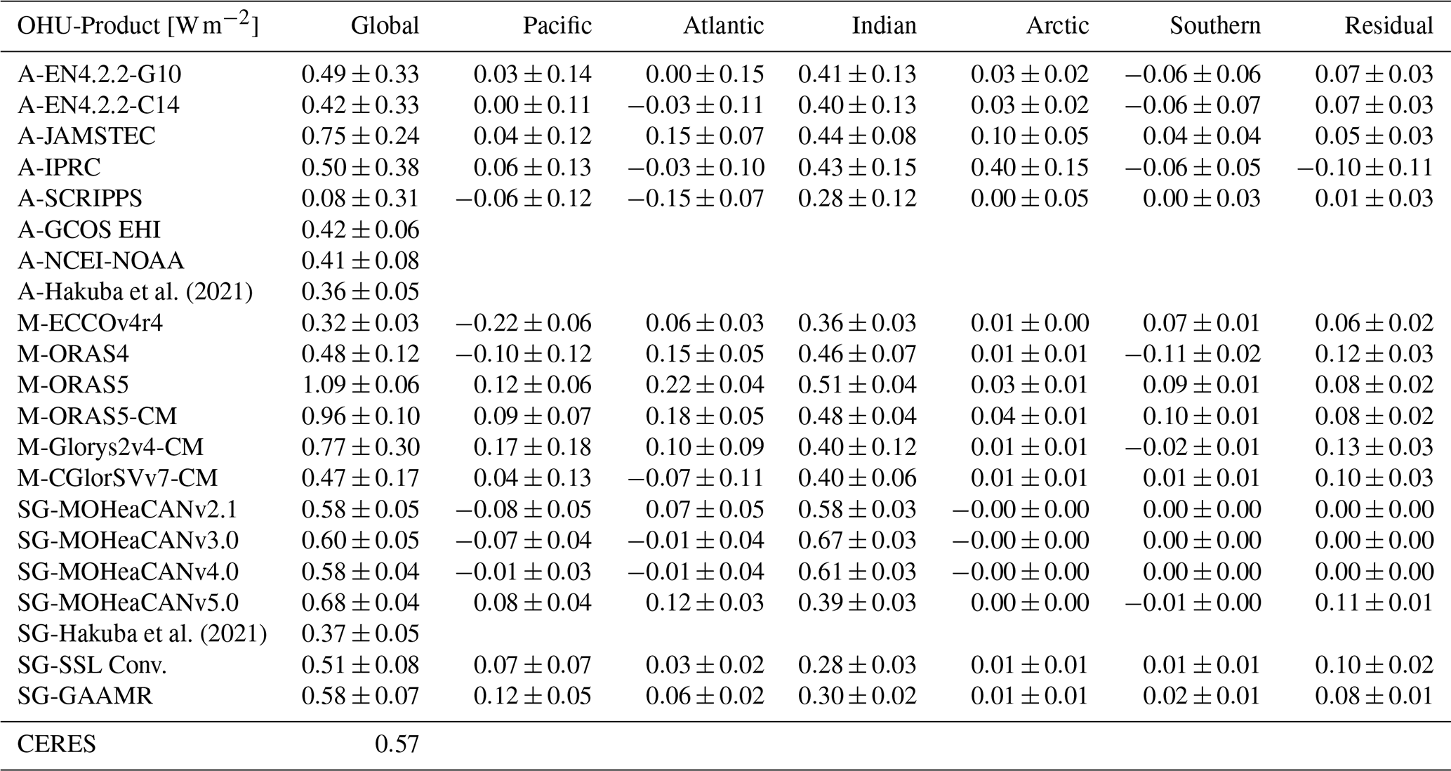
Table A3 Comparison of ocean heat uptake (OHU) trends from individual Argo (A), model/reanalysis (M) and space geodetic (SG) data sources. Analysis period: January 2005 till December 2015. Errors are provided as one sigma values.

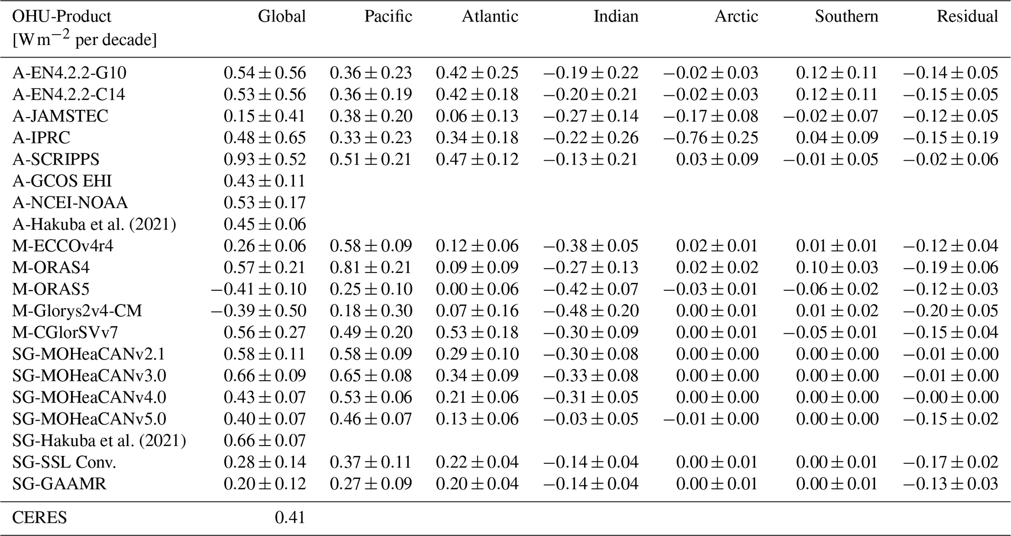
Table A4 Comparison of ocean heat uptake (OHU) from individual Argo (A), model/reanalysis (M) and space geodetic (SG) data sources. Analysis period: January 2005 till December 2015. Results without estimating OHC accelerations, i.e. OHU trends. Errors are provided as one sigma values.

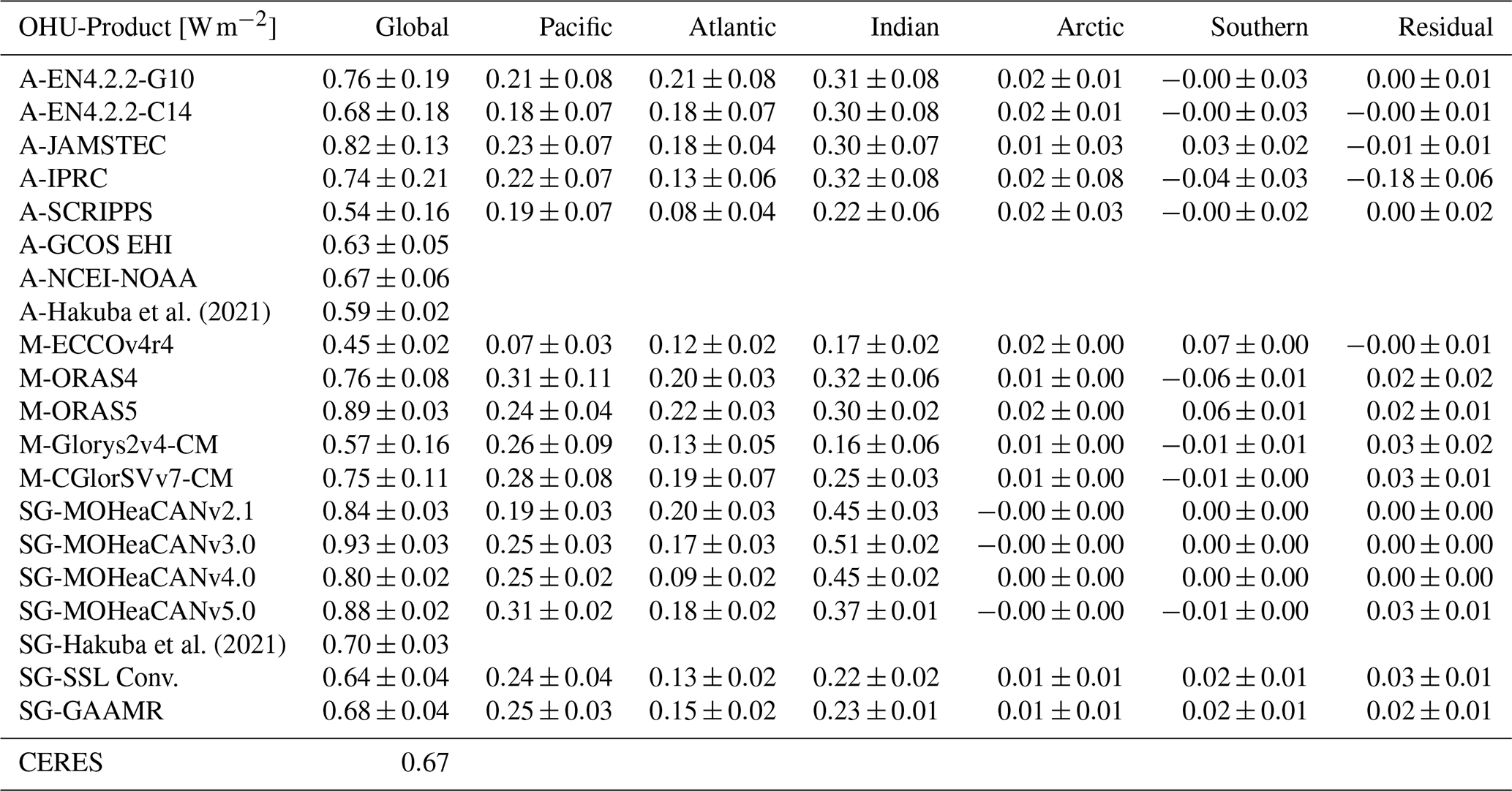
Table A5 Comparison of ocean heat uptake (OHU) from individual Argo (A), model/reanalysis (M) and space geodetic (SG) data sources. Analysis period: January 2005 till December 2024. Errors are provided as one sigma values.

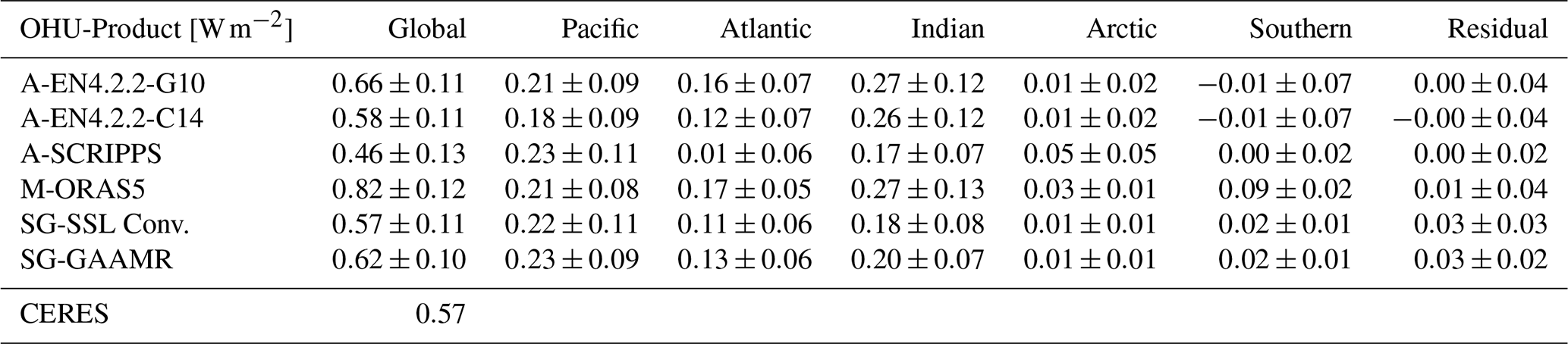
Table A6 Comparison of ocean heat uptake (OHU) trends from individual Argo (A), model/reanalysis (M) and space geodetic (SG) data sources. Analysis period: January 2005 till December 2024. Errors are provided as one sigma values.

Appendix B: Figures

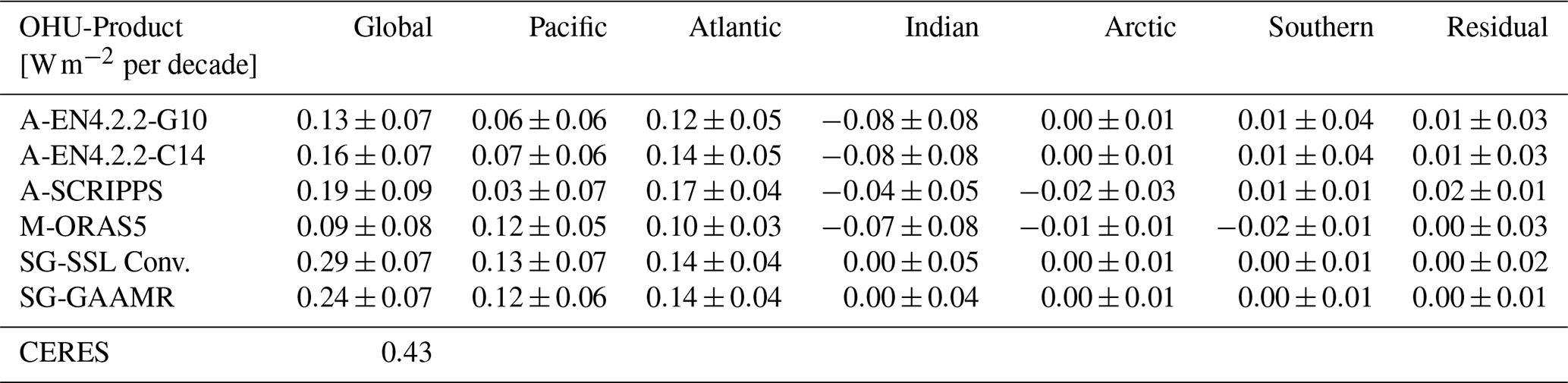
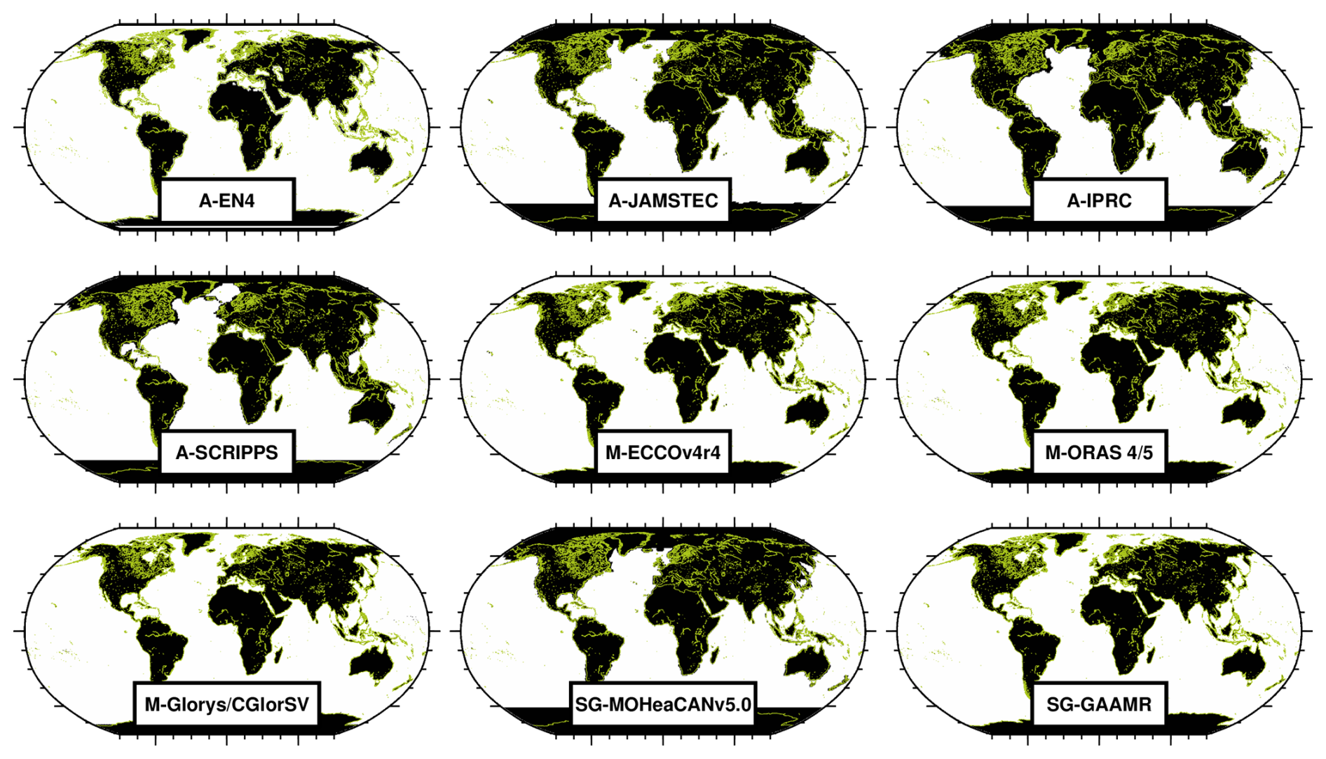
Figure B1 Spatial data coverage for individual data products introduced in Table 1.

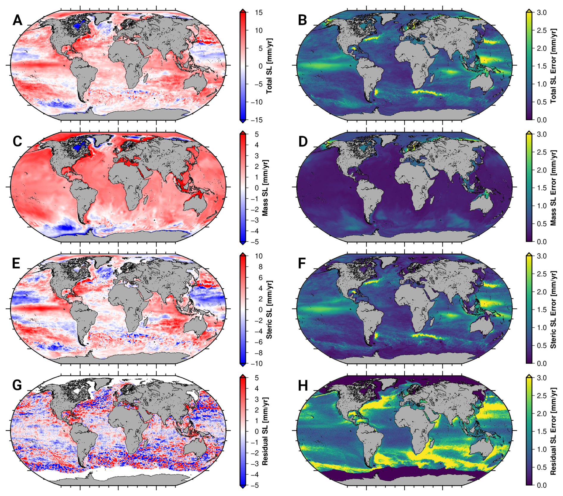
Figure B2 Major regional sea level budget components from the global fingerprint inversion approach. Left column (A, C, E, G) shows the trends from January 2005 till December 2015 and right column (B, D, F, H) shows corresponding trend errors. Note: As the residual component is derived from gridded along-track altimetry residuals, we masked out the area of maximum sea ice extend as seasonally missing along-track altimetry coverage might affect residual trend results in these regions.

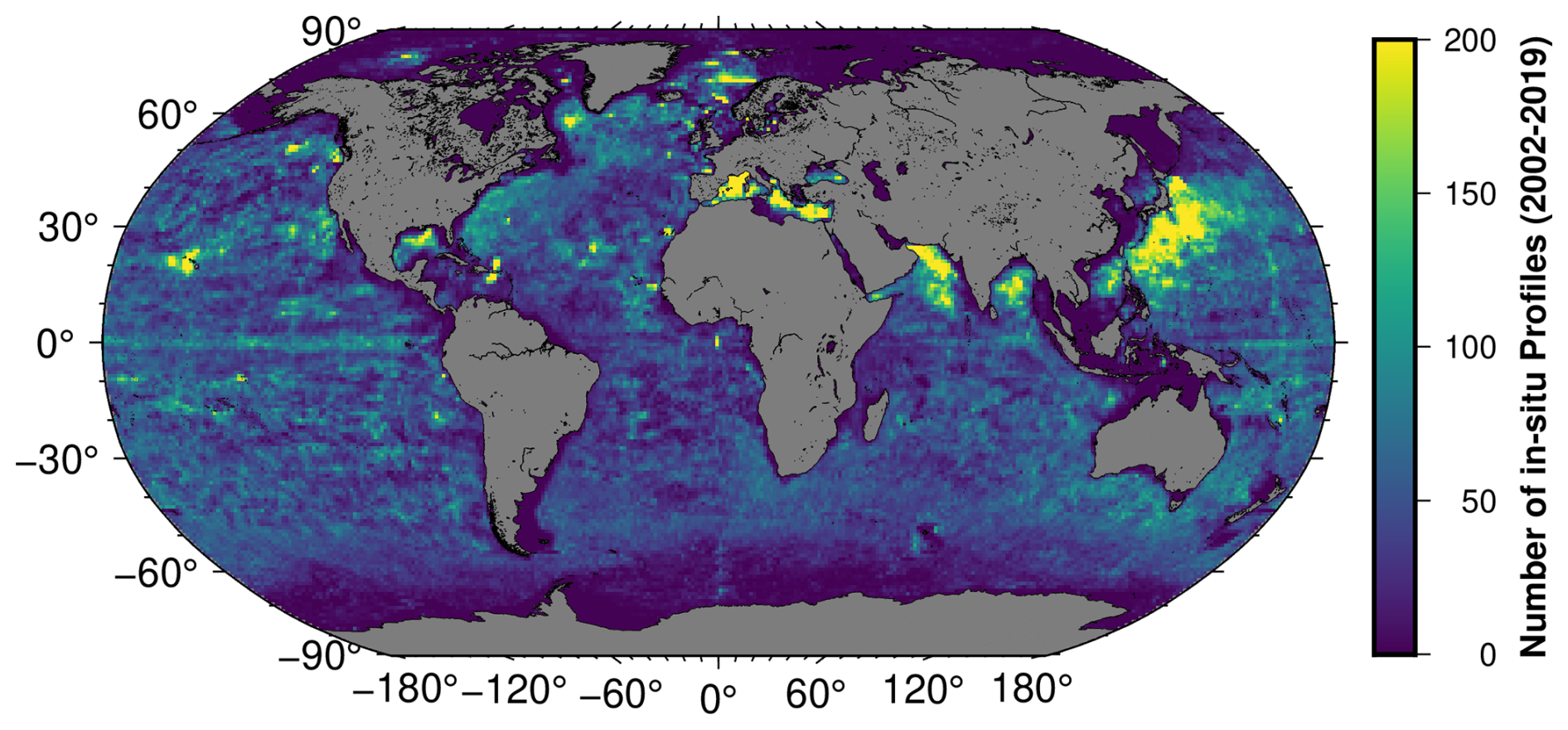
Figure B3 Number of in-situ profiles from the easyCORA datasets between 2002 and 2019 (216 months) at each grid point. The colorscale is capped at 200. Some grid locations may include more than 1000 measurements over the indicated time period.

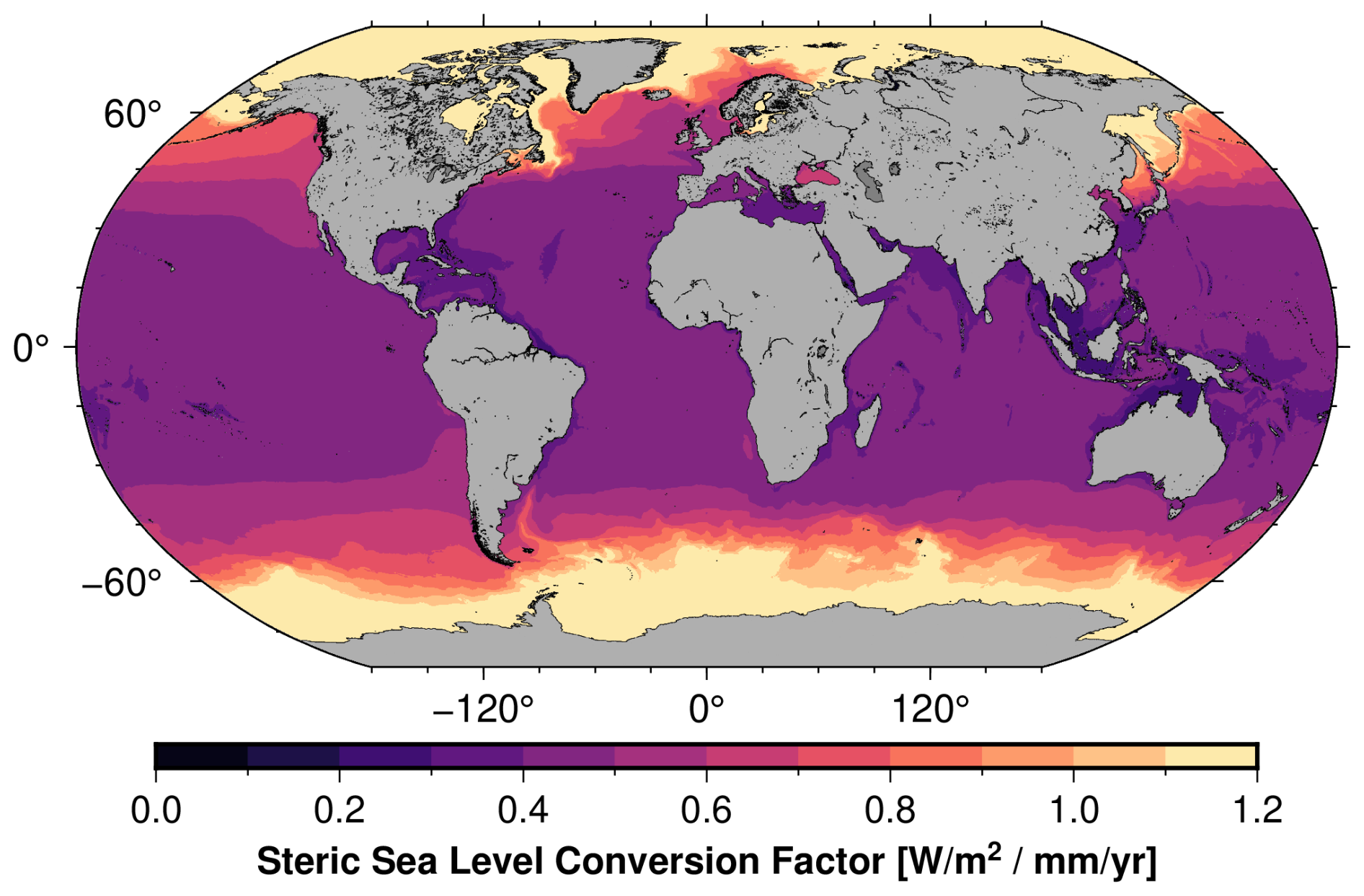
Figure B4 Computing the expansion of heat efficiency following Russell et al. (2000) and based on the ORAS5 ocean reanalyis Zuo et al. (2019) data.