A global hourly ISIMIP3 climate forcing dataset for impact modeling

Sub-daily climate data are increasingly important for climate-impact assessments because many processes, such as heat stress, hydrological extremes, land–surface energy balance, and renewable-energy production, respond non-linearly to intra-day variability. Daily data miss short-duration events and obscure sub-daily inter-variable interactions, creating biases in impact estimates. To address these limitations and provide consistent forcing across sectors, we generated a global hourly climate dataset by temporally disaggregating the Inter-Sectoral Impact Model Intercomparison Project Phase 3 (ISIMIP3) daily climate archives using the Temporal Disaggregation Tool (Teddy). The approach uses analogue-based hourly profiles from the bias-corrected WFDE5 (WATCH Forcing Data methodology applied to ERA5) reanalysis, preserves daily mass and energy, and maintains temporal coherence between variables. We illustrate the utility of the hourly data with four applications using the MPI Earth System Model (MPI-ESM) under ScenarioMIP pathway SSP3–7.0: (1) the fraction of wet hours, revealing rainfall intermittency not captured by daily wet-day metrics; (2) the number of hours with dangerous heat-index values, capturing joint diurnal cycles of temperature and humidity; (3) hours with wind speeds suitable for onshore wind-power generation; and (4) photovoltaic power potential calculated from radiation, temperature, and wind speed at hourly resolution. We discuss the benefits of preserving inter-variable timing, along with limitations such as reduced spatial coherence at sub-daily scales and potential constraints under strong climate-change signals. The resulting hourly ISIMIP3 dataset provides a harmonized foundation for more realistic sub-daily climate-impact modeling across sectors. The dataset is openly available through the ISIMIP repository under the following DOIs: https://doi.org/10.48364/ISIMIP.736682 (Bechtold et al., 2026a) and https://doi.org/10.48364/ISIMIP.170328 (Bechtold et al., 2026b).

1 Introduction

In recent years, sub-daily climate data have become increasingly important in climate-impact analysis, e.g. for simulating solar and wind energy production or agricultural yields (Jägermeyr et al., 2021; Müller et al., 2021, 2024; Schneider et al., 2024), for quantifying human heat stress and the associated loss of labor capacity (Orlov et al., 2024), for representing hydrological fluxes (Huang et al., 2019), and for closing the land–surface energy balance over the diurnal cycle (Renner et al., 2021). To ensure consistency between different scenarios across sectors, the Inter-Sectoral Impact Model Intercomparison Project (ISIMIP, https://www.isimip.org, last access: 25 August 2026) is committed to harmonizing input data shared across different sectors and scales (Warszawski et al., 2014). To guarantee cross-sectoral consistency in ISIMIP, all sectors are provided with the same climate and socioeconomic data for historical (1850–2014) and future time periods (2015–2100) for different Shared Socioeconomic Pathway–Radiative Forcing (SSP–RCP) scenario combinations: SSP1–2.6 (SSP126), SSP3–7.0 (SSP370), and SSP5–8.5 (SSP585). ISIMIP3 provides trend-preserving bias-corrected (Lange, 2019) global climate model data from five different climate models of the Coupled Model Intercomparison Project Phase 6 (CMIP6) (Eyring et al., 2016) and reanalysis climate data (Lange, 2019) at half degree spatial resolution. Within ISIMIP, several modeling communities from different sectors – such as agriculture, energy, and land surface modeling groups of the biome and peat sectors – have expressed a need for sub-daily climate data.

While most climate impact models currently use daily climate model data as an input, sub-daily non-linear interactions cannot be adequately considered at daily time steps. For instance, Orlov et al. (2024) showed that considering labor capacity losses due to heat stress at hourly resolution resulted in up to 30 % higher labor capacity losses for specific regions in comparison to daily aggregated calculations. Furthermore, land surface models require sub-daily rainfall data to accurately simulate the partitioning of precipitation into infiltration and surface runoff. As highlighted by Vereecken et al. (2019), the resolution of rainfall input directly affects the onset of ponding and runoff, and using coarse daily inputs can severely underestimate excess water generation. Hence, hydrological simulations driven by hourly meteorological forcing can better reproduce the intensity of flood peaks compared to simulations driven by daily forcing (Huang et al., 2019), even in catchments where floods are generated by daily to multi-day precipitation rather than by short-duration convective events. Additionally, the energy balance calculations of land surface models are designed for meteorological input data with a diurnal cycle (Renner et al., 2021). These examples demonstrate that hourly data can lead to significantly different results in climate change impact studies.

In this study, we disaggregated daily climate model data from the ISIMIP3a and ISIMIP3b archives to hourly resolution at 0.5° spatial scale using the Temporal Disaggregation Tool (Teddy; Zabel and Poschlod, 2023). ISIMIP3a provides historical simulations driven by observational and counterfactual climate forcing for model evaluation and attribution studies, while ISIMIP3b supplies bias-corrected CMIP6 climate forcing for assessing impacts under different levels of climate change. Section 2 describes the input data used for the disaggregation, and Sect. 3 outlines the Teddy methodology and its implementation for global three-dimensional datasets. In Sect. 4, we present illustrative applications that demonstrate the added value of hourly forcing. Sections 5 and 6 provide information on data and code availability, respectively, and Sect. 7 provides concluding remarks.

2 Data

The daily ISIMIP3a (Lange et al., 2022) data that was temporally disaggregated consist of factual (obsclim) and counterfactual (counterclim) climate data for 20CRv3 (1901–2015), 20CRv3-ERA5 (1901–2024 for obsclim and 1901–2019 for counterclim), 20CRv3-W5E5 (1901–2019), and GSWP3-W5E5 (1901–2019). The counterclim data are a detrended version of the associated obsclim data, where the detrending is done using version 1.1 of the ATTRICI method (Mengel et al., 2021). In addition, a 50-year climate dataset for the transition of a spin-up period to counterclim or obsclim is provided for GSWP3-W5E5 (1851–1900).

The GSWP3-W5E5 dataset is based on GSWP3 v1.09 (Kim, 2017) and W5E5 v2.0 (Cucchi et al., 2020; Lange et al., 2021). The GSWP3 dataset is a dynamically downscaled and bias-adjusted version of the Twentieth Century Reanalysis version 2 (20CRv2) (Compo et al., 2011). The W5E5 dataset is a bias-adjusted version of the European Reanalysis (ERA5) (Hersbach et al., 2020). The GSWP3-W5E5 data combines W5E5 for the time period 1979–2019 with GSWP3 bias-adjusted towards W5E5 for the time period 1901–1978. The bias adjustment is done using ISIMIP3BASD (Lange, 2019). The 20CRv3-W5E5 dataset is based on W5E5 v2.0 and ensemble member 1 of the Twentieth Century Reanalysis version 3 (20CRv3) (Slivinski et al., 2019, 2021) interpolated to 0.5° spatial resolution. 20CRv3-W5E5 is a combination of W5E5 for the time period 1979–2019 with 20CRv3 bias-adjusted (using ISIMIP3BASD) towards W5E5 for the time period 1901–1978. The 20CRv3-ERA5 dataset is similar to 20CRv3-W5E5, but using ERA5 instead of W5E5 for the time period 1979–2021. The 20CRv3 dataset is ensemble member 1 of 20CRv3 interpolated to 0.5° spatial resolution but not bias-adjusted to any other dataset.

The daily ISIMIP3b data that was temporally disaggregated consist of five harmonized and bias-corrected CMIP6 climate model datasets (GFDL-ESM4, IPSL-CM6A-LR, MPI-ESM1-2-HR, MRI-ESM2-0 and UKESM1-0-LL), which were downscaled to half degree spatial resolution using the same grid for all climate models and bias-corrected toward the GSWP3-W5E5 data for an extended historical (1850–2014) period and three different scenarios (SSP126, SSP370, and SSP585) for future time periods (2015–2100). The historical period follows the CMIP6 historical experiment and the future periods follow the corresponding ScenarioMIP SSP–RCP combinations, with the bias adjustment and statistical downscaling from the native climate model grids to the common 0.5° grid performed per climate model and variable with ISIMIP3BASD (Lange, 2019) using GSWP3-W5E5 as the observational reference. The five climate models were selected from the CMIP6 ensemble by ISIMIP on the basis of the availability of all variables required by the impact models at daily resolution over the full period 1850–2100, the performance of the models over the historical period, their structural independence in terms of atmosphere and ocean components, an expert assessment of their process representation, and their equilibrium climate sensitivity, such that both the mean and the spread of the equilibrium climate sensitivity of the full CMIP6 ensemble are represented by the selected subset (Frieler et al., 2026). The temporal disaggregation is applied for climate data on land; oceans are masked out since no hourly reference reanalysis data are available.

3 Methods

Teddy (v1.1) has been described and validated in detail by Zabel and Poschlod (2023) for point applications, i.e., applications carried out at the scale of individual grid cells. To apply Teddy for huge three-dimensional (lat, lon, time) climate data, the tool was parallelized to enhance model performance. Teddy requires simultaneous access to all climate variables. Due to the large global data volume of the various climate variables, it was necessary to manage the amount of data held in RAM. To control the required RAM size, Teddy operates with zonal strips that are processed sequentially from north to south. The size of the strips (number of rows) can be adjusted according to the size of the available working memory. The striping serves only for memory management and computational efficiency and does not modify the analogue-search algorithm: the most similar meteorological day is determined independently for every individual grid cell from the reference record at that same location, so the selected analogue day does not depend on the strip in which a grid cell is processed. Teddy v1.3 additionally allows users to define a bounding box that specifies the spatial extent of the calculations. All new developments have been published (see Sect. 6).

The methodology for temporal disaggregation in Teddy is based on the choice of daily climate analogues. As a reference, globally available bias-corrected hourly reanalysis WFDE5 (WATCH Forcing Data methodology applied to ERA5) data from 1980–2019 (Cucchi et al., 2020) are used to take specific local and seasonal features of the empirical diurnal profiles into account. For a given location and day within the climate model data, the Teddy tool screens the reference dataset to find the most similar meteorological day based on rank statistics. The diurnal profile of the reference data is then applied to the climate model. Thereby, mass and energy are strictly preserved to exactly reproduce the daily values from the climate models. The physical dependency between variables is preserved, since the diurnal profile of all variables is taken from the same, most similar meteorological day of the reference dataset. A validation showed that Teddy is able to reproduce historical diurnal courses with high correlations >0.9 for all variables, except for wind speed (>0.75) and precipitation (>0.5) (Zabel and Poschlod, 2023). The weaker performance for wind speed and precipitation reflects their larger intrinsic stochastic variability at sub-daily scales (Görner et al., 2021). Temperature, relative humidity and radiation are governed by a strong and highly reproducible radiative diurnal cycle and are correspondingly autocorrelated within the day, so that a day with similar daily statistics also tends to have a similar diurnal course. Precipitation and near-surface wind speed, in contrast, are dominated by intermittent, event-driven processes whose timing within the day is only weakly constrained by the daily aggregate, so that an analogue day matching the daily statistics does not necessarily reproduce the intra-day timing of individual rainfall or gust events. The same ordering of variables by disaggregation skill is reported for other temporal disaggregation approaches (Förster et al., 2016).

Teddy applies the diurnal profiles and intraday variability from the WFDE5 data. Thus, the disaggregation process in Teddy is consistent with the bias adjustment in ISIMIP3 (Lange, 2019), which uses the same reference data.

Data processing has been performed on the Tier-1 Cluster of the High Performance Computing system of the Vlaams Supercomputer Center. The temporal disaggregation required approximately 7 million CPU hours. The hourly data is provided as 5-year NetCDF files. After reducing the numeric precision, the hourly files amount to 16 TB in total.

For the disaggregation of daily ISIMIP climate model data, we use specific settings. In Teddy, a day of year (DOY) window to find the most similar historical reference weather situations can be chosen in different sizes. Zabel and Poschlod (2023) evaluated different DOY window sizes and generally found small effects of time window adjustments for most of the variables, except for precipitation and wind speed. They suggested that a DOY window size of 11 can generally be recommended across all variables, because shorter DOY windows decrease the probability to find analogue weather situations in the historical reference data and could therefore lead to poorer representations of autocorrelation and extreme events, while larger DOY windows can be problematic in arid regions during the rainy season. Therefore, we follow the recommended DOY window size of 11 d. In addition, Teddy is applied with the option to consider the inter-day connectivity of precipitation (Li et al., 2018). Depending on the precipitation state of the previous day, the day of interest, and the following day, Teddy considers eight classes, namely dry–dry–dry, dry–dry–wet, wet–dry–dry, wet–dry–wet, dry–wet–dry, dry–wet–wet, wet–wet–dry, and wet–wet–wet. Only days with the same precipitation class as the climate model day of interest are selected in the historical reference data. Despite accounting for inter-day connectivity through the wet/dry classification, discontinuous jumps between consecutive days may still occur in the hourly sequence, as the analogue daily profiles originate from different reference days.

Table 1 shows the hourly output variables of Teddy. Note that two variables of the ISIMIP daily data are missing: snowfall and specific humidity (huss). The consistent disaggregation of snowfall in a way that aligns with the disaggregated precipitation and temperature, while preserving temporal coherence across variables, is not straightforward but a key aim of Teddy. However, snowfall can be estimated from hourly temperature and precipitation data. In a global assessment, we found that using a temperature threshold of 1.5 °C yielded snowfall totals from the hourly data that closely matched the daily data. Specifically, if T≤1.5 °C and P>0, then Snowfall=P. The other lacking variable is specific humidity (variable huss in ISIMIP). This was not derived by disaggregation to reduce data redundancy and can be directly calculated from hourly pressure, temperature, and relative humidity data.

Table 1 Output variables at 1 h temporal resolution.

4 Illustrative applications

We illustrate the capabilities of the disaggregated hourly dataset for four different impact-related metrics covering a wide range of output variables. The calculations are based on the MPI-ESM under SSP370 comparing the reference period (1981–2010) to the far future (2071–2100).

4.1 Fraction of wet hours

The fraction of wet hours provides insight into the frequency and persistence of rainfall events, rather than just their intensity or total volume. It is relevant for hydrological assessments, such as the evaporative loss of intercepted rainfall (Lian et al., 2022). Here, we apply the threshold of 0.1 mm h⁻¹ following Ban et al. (2015) and map the global distribution of wet hours and their change until the end of the century (see Fig. 1). The spatial distribution shows high heterogeneity, with values ranging from just above 0 in desert areas to 0.65 in the tropics (Fig. 1a). The far future projection indicates a considerable decrease of wet hours in the Amazon region, Central and North America, and the Mediterranean region, while the northern latitudes, Northern India and parts of the African and Asian tropics are projected to get a higher fraction of wet hours. The general spatial pattern of Fig. 1a is similar to the wet-day frequency, with a threshold of 1 mm d⁻¹ (McErlich et al., 2023). However, the hourly assessment better accounts for climates, where short-duration rainfall events largely contribute to the annual rainfall volume. At daily resolution, each day with a short-duration event above the volume of 1 mm is counted as “wet”, whereas the hourly assessment only considers the time of the short-duration event.

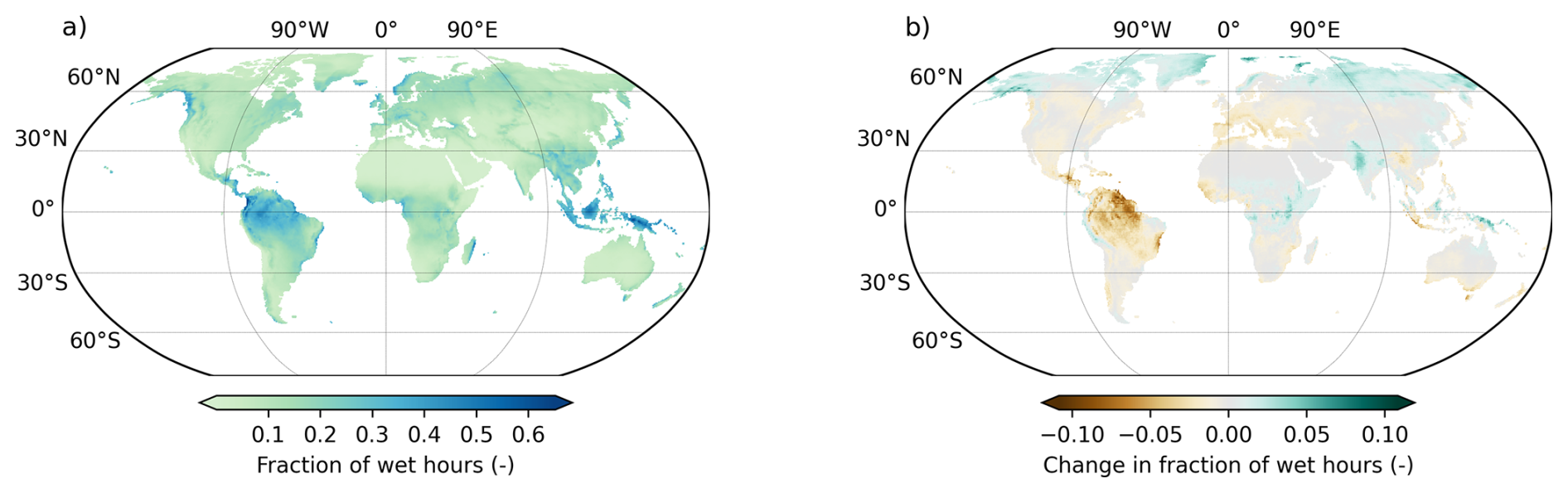
Figure 1 (a) Fraction of wet hours in 1981–2010 based on the MPI-ESM. (b) Change of the fraction of wet hours until 2071–2100 under SSP370. This analysis is available for the full set of ISIMIP3 climate models and scenarios from Poschlod and Zabel (2025c).

4.2 Number of hours with dangerous heat index

The NOAA heat index is a measure used to quantify heat stress for humans, which considers the combined effect of temperature and relative humidity (Rothfusz, 1990; Steadman, 1979). The heat index is based on a multiple linear regression using temperature and relative humidity as input and is itself expressed as temperature value (Schwingshackl et al., 2021). It is often referred to as an estimation of “apparent temperature” (Anderson et al., 2013). The United States' National Weather Service categorizes heat index values above 103 °F (39.4 °C) as “dangerous” as it can cause heat exhaustion and heat cramps (Vargas Zeppetello et al., 2022). Here, we apply this threshold to the hourly disaggregated data to map the number of dangerous hours per year based on the reference period (Fig. 2) and its change until the end of the century (Fig. 2b). In the tropical regions, over 1500 h yr⁻¹ are reached on average. The warming under SSP370 until 2071–2100 leads to strong increases of dangerous heat conditions with annual hours more than doubling in the tropics. Furthermore, the regions affected by dangerous heat conditions extend poleward (Fig. 2b). While existing global studies are often based on daily temperature or daily maximum temperature (Schwingshackl et al., 2021; Vargas Zeppetello et al., 2022), the disaggregated data allow for a consideration of the joint diurnal cycle of temperature and relative humidity, thereby enabling a more detailed analysis of human exposure to dangerous heat conditions. Orlov et al. (2024) show that using hourly instead of daily values can drastically change impact assessments illustrating the loss of human labor capacity in the agricultural sector due to heat stress.

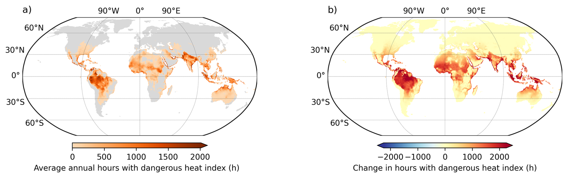
Figure 2 (a) Average annual number of hours with a “dangerous” heat index above 103 °F (39.4 °C) in 1981–2010 based on the MPI-ESM. (b) Change of the number of hours until 2071–2100 under SSP370. This analysis is available for the full set of ISIMIP3 climate models and scenarios from Poschlod and Zabel (2025a).

4.3 Suitable conditions for onshore wind power generation

Wind turbines operate only within a defined range of wind speeds, characterized by a lower threshold, the cut-in wind speed, at which power generation commences, and an upper threshold, the cut-out wind speed, beyond which turbines are shut down to prevent mechanical damage and ensure operational safety. For the reference turbine IEA 3.4 MW at a hub height of 80 m (Bortolotti et al., 2019) a cut-in wind speed of 4 m s⁻¹ and a cut-out wind speed of 25 m s⁻¹ are reported, respectively. Between the cut-in wind speed and the rated wind speed, the power extracted by a turbine increases approximately with the cube of the wind speed (Bosch et al., 2017). Wind power generation therefore responds strongly non-linearly to sub-daily wind speed variations and cannot be recovered from daily mean wind speeds, which is why the metric presented here is deliberately restricted to the frequency of suitable conditions rather than to the generated power. For the hourly ISIMIP wind speed data v₁₀ at 10 m above the surface, we apply a simple power law transformation following Miao et al. (2023) to empirically derive wind speeds v₈₀ at 80 m above the surface:

$$\begin{array}{}\text{(1)}& v_{\mathrm{80}}=v_{\mathrm{10}}{\left({\displaystyle \frac{\mathrm{80}}{\mathrm{10}}}\right)}^{\mathrm{0.14}}\end{array}$$

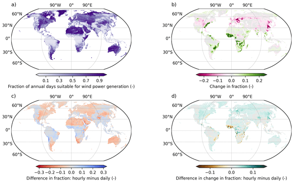
We assess the fraction of hours globally, where v₈₀ is within the cut-in and cut-out wind speed thresholds and is therefore suitable for wind power generation (Fig. 3). The tropics show a high frequency of low wind speeds. Furthermore, the spatial pattern of suitable hours is affected by topographic effects of complex terrain and land-sea interaction at the coastlines (Fig. 3a). The projections of the MPI-ESM indicate an increase of suitable wind speeds in the South American and African tropics as well as the east coast of the United States, while showing decreases in Europe and Eastern Asia. However, Miao et al. (2023) note that future projections of wind speed show a high degree of model and scenario uncertainty.

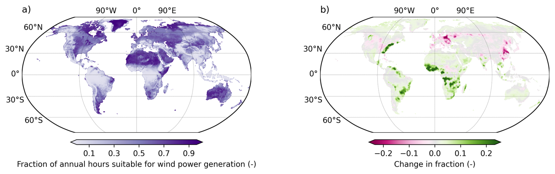
Figure 3 (a) Fraction of annual number of hours suitable for wind power generation in 1981–2010 based on the MPI-ESM. (b) Change of the fraction until 2071–2100 under SSP370. This analysis is available for the full set of ISIMIP3 climate models and scenarios from Poschlod and Zabel (2025d).

Early global wind power potential assessments were based on average wind speed (Bandoc et al., 2018) or on 6-hourly reanalysis data (Lu et al., 2009), whereas more recent assessments derive temporally explicit global onshore wind energy potentials directly from hourly reanalysis wind speeds (Bosch et al., 2017). Climate change effects on wind power generation, in contrast, are still estimated from daily global climate model data (Miao et al., 2023). The disaggregated hourly data help to close this gap, because they capture the sub-daily variability of wind speeds needed for a realistic global assessment of wind power generation and are at the same time available for the full set of ISIMIP3 climate models and scenarios. Renewable-energy potential assessments and climate-impact assessments can thus be driven by one and the same bias-adjusted, temporally consistent forcing.

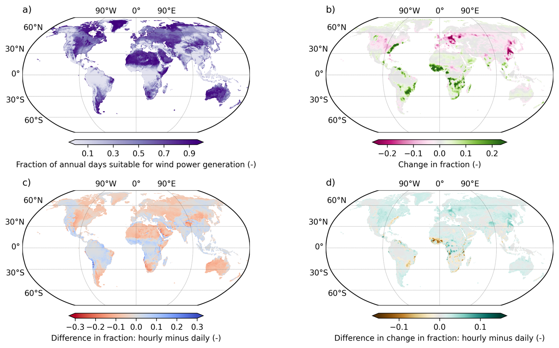
Figure 4 Comparison of the assessment of suitable conditions for wind power generation based on daily and on hourly climate data. (a) Fraction of annual number of days suitable for wind power generation in 1981–2010 based on the daily MPI-ESM data (same color scale as Fig. 3a). (b) Change of the fraction until 2071–2100 under SSP370 based on daily data (same color scale as Fig. 3b). (c) Difference of the fraction in 1981–2010, hourly minus daily. (d) Difference of the projected change, hourly minus daily.

To illustrate the order of magnitude in which hourly and daily assessments differ, we repeat this analysis with the daily mean wind speed of the same climate model data, i.e. counting suitable days instead of suitable hours (Fig. 4). In regions with generally high wind speeds, such as North America, the Sahara–Arabian belt and Australia, the daily assessment yields a considerably higher fraction of suitable time steps, because the daily mean exceeds the cut-in wind speed on most days while a substantial share of the individual hours does not (negative differences in Fig. 4c). In the humid tropics the sign reverses: there the daily mean rarely reaches the cut-in wind speed, whereas the hourly data still resolve individual hours with sufficient wind, so that the hourly assessment gives the higher fraction. The projected climate change signal is less sensitive to the temporal resolution of the forcing, but regionally, in particular in the African and South American tropics, the differences reach a magnitude comparable to the signal itself (Fig. 4d).

4.4 Photovoltaic power potential

The photovoltaic power potential (PV_pot) represents a dimensionless indicator quantifying the performance of photovoltaic cells relative to their nominal power capacity, as determined by prevailing meteorological conditions. Accordingly, the product of PV_pot and the nominal installed photovoltaic capacity yields the photovoltaic power output (Jerez et al., 2015). We estimate PV_pot based on surface-downwelling shortwave radiation (rsds) considering the influence of temperature and wind speed on the solar panel efficiency following Jerez et al. (2015):

$$\begin{array}{}\text{(2)}& {\mathrm{PV}}_{\mathrm{pot}}\left(t\right)=P_{\mathrm{R}}\left(t\right){\displaystyle \frac{\mathrm{rsds}\left(t\right)}{{\mathrm{rsds}}_{\mathrm{STC}}}}\end{array}$$

where rsds_STC refers to the standard test conditions of a solar panel (rsds_STC=1000 W m⁻²). P_R is the performance ratio considering the influence of the estimated photovoltaic cell temperature T_cell on the panel efficiency:

$$\begin{array}{}\text{(3)}& P_{\mathrm{R}}\left(t\right)=\mathrm{1}+\mathit{\gamma }\left(T_{\mathrm{cell}}\left(t\right)-T_{\mathrm{STC}}\right)\end{array}$$

where T_STC=25 °C and γ equals −0.005 °C⁻¹ in accordance with the response of monocrystalline silicon solar panels (Tonui and Tripanagnostopoulos, 2008). The photovoltaic cell temperature T_cell is empirically modeled based on surface-downwelling shortwave radiation, temperature (tas), and wind speed (v₁₀):

$$\begin{array}{}\text{(4)}& T_{\mathrm{cell}}=c_{\mathrm{1}}+c_{\mathrm{2}}\mathrm{tas}\left(t\right)+c_{\mathrm{3}}\mathrm{rsds}\left(t\right)+c_{\mathrm{4}}{v}_{\mathrm{10}}\left(t\right)\end{array}$$

where c₁=4.3 °C, c₂=0.943, c₃=0.028 °C m² W⁻¹, and $c_{\mathrm{4}}=-\mathrm{1.528}$ °C s m⁻¹ according to Chenni et al. (2007). If the meteorological conditions in Eq. (4) lead to the standard test condition of T_cell=25 °C and rsds=1000 W m⁻², PV_pot equals 1. Figure 5a presents the global distribution of annual average PV_pot based on hourly ISIMIP data of the MPI-ESM in 1981–2010. Under SSP370, increases by 5 %–10 % are projected for Europe, the eastern part of the United States and the Amazon region (Fig. 5b). Notable decreases are projected in tropical Africa, India, Alaska, Canada and Greenland. Other global assessments of climate change effects on the photovoltaic power potential are based on annual (Wild et al., 2015) or daily (Crook et al., 2011) climate data. The hourly disaggregated data allow better capture of the inter-variable dependencies in the diurnal cycle, which allows the cell temperature and performance ratio to be modeled.

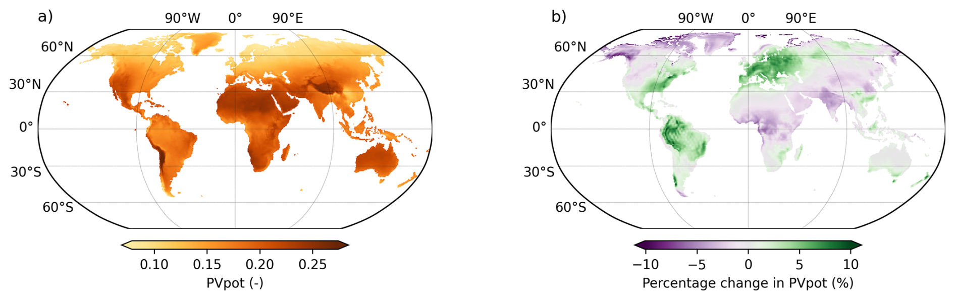
Figure 5 (a) Photovoltaic power potential (PV_pot; dimensionless) in 1981–2010 based on the MPI-ESM. (b) Percentage change of PV_pot until 2071–2100 under SSP370. This analysis is available for the full set of ISIMIP3 climate models and scenarios from Poschlod and Zabel (2025b).

This example is a simple illustration of a possible application. The calculation refers to a horizontal plane, and rsds is used as provided, i.e. without separating it into its direct and diffuse components and without transposing the radiation onto the plane of an inclined or sun-tracking array. A realistic assessment of installed photovoltaic systems requires both steps, and the resulting values of PV_pot would differ, in particular at high latitudes and for tracking systems. Such a treatment depends on the position of the sun and on the sub-daily evolution of the radiation components and can therefore only be carried out with sub-daily forcing data, so that the hourly dataset is a prerequisite for a more complete photovoltaic assessment.

As for the wind power example, we repeated the calculation of PV_pot with daily mean values of rsds, tas, and v₁₀ (Fig. 6). Across all land regions, PV_pot derived from hourly data is lower than PV_pot derived from daily means (Fig. 6c). This is a direct consequence of the non-linear coupling between radiation and cell temperature in Eqs. (2)–(4): the daily mean radiation is much lower than the radiation actually received around midday, so that the daily calculation underestimates the cell temperature and thus overestimates the performance ratio during the hours in which most of the energy is generated. The temporal resolution of the forcing also affects the projected climate change signal, which is systematically more positive when computed from hourly data over nearly all land areas (Fig. 6d). Both examples show that the differences between daily and hourly forcing are not restricted to the representation of short-duration events but propagate into the projected changes themselves.

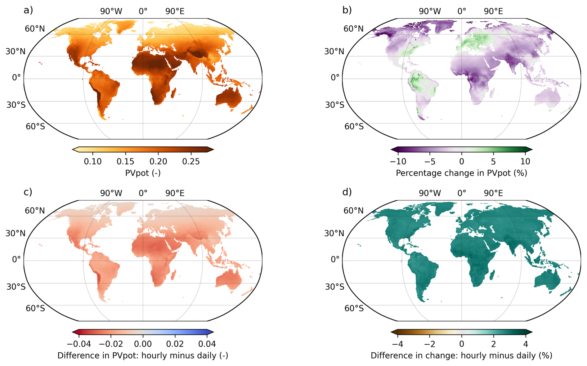
Figure 6 Comparison of the photovoltaic power potential (PV_pot) calculated from daily and from hourly climate data. (a) PV_pot in 1981–2010 based on the daily MPI-ESM data (same color scale as Fig. 5a). (b) Percentage change of PV_pot until 2071–2100 under SSP370 based on daily data (same color scale as Fig. 5b). (c) Difference of PV_pot in 1981–2010, hourly minus daily. (d) Difference of the projected percentage change, hourly minus daily.

5 Data availability

Data described in this manuscript can be accessed at the ISIMIP Repository under the following data DOIs: https://doi.org/10.48364/ISIMIP.736682 (Bechtold et al., 2026a) and https://doi.org/10.48364/ISIMIP.170328 (Bechtold et al., 2026b).

The dataset is provided at hourly resolution only. Users whose impact models operate at coarser sub-daily time steps, or who only require a limited region, are advised to process the archive sequentially. The data are organized as 5-year NetCDF files per variable, so that each file can be retrieved, aggregated to the required sub-daily time step and cropped to the area of interest before the next one is processed. In this way only the aggregated or cropped output has to be stored.

6 Code availability

The model code is openly available as Teddy v1.3 on GitHub (https://github.com/flozabel/Teddy, last access: 25 August 2026) and Zenodo (https://doi.org/10.5281/zenodo.17551135; Zabel and Poschlod, 2025).

7 Conclusions

Although General Circulation Models (GCMs) internally operate at sub-hourly time steps to resolve atmospheric dynamics, their standard archived outputs in CMIP6 – and thus in ISIMIP – are typically provided only at daily resolution due to storage constraints. Consequently, no globally consistent, bias-corrected hourly climate projections are available to the impact modeling community through standard data portals, despite strong demand from sectoral models. Temporal disaggregation of daily fields therefore represents a necessary step to derive hourly forcing data. Moreover, directly using raw hourly GCM output for climate impact modeling is not necessarily preferable, as many sub-daily processes are not reliably represented at coarse spatial resolution and would require additional bias correction. Our approach instead constrains sub-daily variability using bias-corrected hourly reanalysis data (WFDE5) as a reference, which has previously been shown to reproduce realistic diurnal structures and variability patterns (Zabel and Poschlod, 2023). The hourly WFDE5 reference data are bias-adjusted using the same methodology as the daily ISIMIP3a and ISIMIP3b climate model datasets (Lange, 2019), ensuring conceptual consistency between the corrected daily projections and the hourly reference used to reconstruct sub-daily variability.

This study provides a comprehensive global hourly climate forcing dataset for the Inter-Sectoral Impact Model Intercomparison Project Phase 3 (ISIMIP3), enabling impact modelers across sectors to incorporate sub-daily variability that is essential for capturing non-linear processes and diurnal dynamics. By applying the Temporal Disaggregation Tool (Teddy) to daily ISIMIP3 forcing, we deliver hourly meteorological fields that are consistent with ISIMIP’s bias-correction framework and suitable for cross-sectoral impact assessments. For two of the four illustrative applications, we additionally quantified how the results change when the same metric is computed from daily instead of hourly forcing (Sect. 4.3 and 4.4). These comparisons show that the temporal resolution of the forcing affects both the magnitude of the impact metric and its projected climate change signal, and that the sign of the effect is metric- and region-dependent, so that it cannot be anticipated from the daily data alone.

The disaggregation methodology strictly preserves mass and energy to exactly reproduce the daily values from the climate models. Compared to other methodologies that disaggregate each variable independently, Teddy additionally preserves the temporal co-occurrence and relationships between meteorological variables, since the diurnal profiles of all variables are derived from the same, most similar meteorological day in the historical reanalysis dataset. This temporal coherence is particularly relevant for processes that depend on the simultaneous interaction of variables, such as the calculation of evapotranspiration, where the balance between solar radiation, air humidity, and precipitation determines the actual evaporative fluxes during and after rainfall events. However, the temporal coherence between the variables comes at the expense of spatial correlation, which is not guaranteed at hourly time steps in Teddy. The methodology makes use of historical reference data, which allows to take regional and seasonal climate features of daily cycles into account, implicitly assuming that these remain valid under future climate scenarios.

Another limitation of the methodology could occur in the case of strong climate change signals. In end-of-century projections with strong warming, the number of unique sampled historical days might decrease because the same reference days may be selected repeatedly. Zabel and Poschlod (2023) showed for SSP370 using the GFDL-ESM4 climate model that the number of unique analogue climate days is declining, as expected, but still the diversity of chosen days is above 300 unique days at the end of the century for a chosen moving window size of ±11 d. A decreasing number of unique analogues does not translate directly into a corresponding loss of variability in the disaggregated fields. Because Teddy conserves the daily mass and energy of the climate model, the repeated use of the same analogue profile still yields different diurnal courses, with a different offset and a different amplitude for each day. What the approach cannot represent is a genuine change in the shape of the diurnal cycle itself, for instance a shift in the timing of convective rainfall or a change in the diurnal temperature range that is not already contained in the historical reference period. Several aspects should be weighed when judging how relevant this is for a given application: the magnitude of the warming signal and thus how far the projected daily statistics move outside the range covered by the reference period; the variable of interest, since the diurnal cycles of temperature and radiation are more strongly constrained by the astronomical forcing than those of precipitation and wind speed; and the uncertainty of the climate projections themselves, which for most variables and regions remains substantial at the end of the century. The properties of the alternative also matter: native sub-daily output of global climate models is archived only for a limited subset of models, variables and experiments in CMIP6, it is not bias-adjusted, and, as mentioned above, it does not reliably resolve sub-daily processes at the coarse spatial resolution of the models.

Zabel and Poschlod (2023) showed that the precipitation data disaggregated with Teddy can reproduce the exceedance probabilities of the hourly WFDE5 data very well across the entire range of different intensities. However, there is a tendency to overestimate the intensity of rare hourly events, such as the annual maxima of hourly precipitation. Beyond the disaggregation itself, the hourly precipitation intensities are constrained by those of the WFDE5 reference. The bias adjustment applied in WFDE5 acts on monthly precipitation totals and on the monthly number of wet days (Cucchi et al., 2020), so that the distribution of intensities within the day is inherited from ERA5, which tends to produce precipitation too frequently and at too low intensities and to underestimate the highest hourly rates (Lavers et al., 2022). Absolute hourly rainfall intensities from the disaggregated data should therefore be interpreted with care.

Consistent with this, and given the spatial resolution of the dataset of 0.5° × 0.5°, we do not recommend the disaggregated hourly data to be used for the analysis of extreme events happening on small scales. This applies for flash floods, i.e. floods that develop in catchments smaller than a few hundred square kilometers and on timescales of at most a few hours (Borga et al., 2011). A single grid cell of the dataset covers up to about 3000 km², and the underlying climate model information originates from global models with native resolutions on the order of 100 × 100 to 250 × 250 km². We do argue, however, that the data disaggregation adds value for assessments of global water balance (Boulange et al., 2023) and for flood simulations of large catchments (Jiang et al., 2023), in which floods are driven by daily to multi-day precipitation. There, the hourly resolution improves the representation of the diurnal cycle and therefore of the energy balance and land surface processes, and it resolves sub-daily process distinctions that matter for runoff generation, such as daytime rainfall versus overnight snowfall and the sub-daily dynamics of snowmelt. This is the sense in which the hourly data can improve hydrological flood simulations.

A further constraint of the present dataset is its restriction to land. The disaggregation relies on the bias-adjusted hourly WFDE5 reference, which is available over land only, and keeping to this reference preserves the consistency with the ISIMIP bias-adjustment framework. It does, however, limit applications that require onshore and offshore resources within a single modeling framework, such as energy-system studies that include offshore wind. An extension of the disaggregation to the oceans using raw hourly ERA5 (Hersbach et al., 2020) as the reference is technically feasible and is a plausible route for a future version of the dataset. The offshore fields would then not be bias-adjusted and would consequently not be fully consistent with the land fields, which is a trade-off that would have to be documented and taken into account by users.

Overall, the new hourly ISIMIP3 dataset substantially expands the analytical possibilities for impact modeling by providing a harmonized, physically consistent, and globally complete sub-daily forcing product. While users should keep mentioned methodological limitations in mind, the dataset offers an important step forward for more realistic quantification of climate-change impacts across sectors and spatial scales.