Global satellite gravity data products for prompt detection of short-term Mass Change (MC)

We present the globally available dataset of Line-of-sight Gravity Differences (LGD) as a new data product to fill the long-standing gap of investigating sub-monthly surface mass change from the satellite gravimetry along-track perspective. The dataset is generated directly from Gravity Recovery and Climate Experiment Follow-on (GRACE-FO) Level-1B intersatellite ranging observations, positioned conceptually between Level-1B measurements and Level-2 monthly gravity field solutions. Provided as along-track time series, LGD delivers instantaneous gravity change at satellite altitude, thus ensuring the fidelity of measurements by avoiding the complex preprocessing, regularization, and filtering applied to monthly products. The instantaneous LGD measurements enable monitoring of sub-monthly terrestrial water storage variability and provide accurate information on timing and magnitude of water mass changes. GRACE-FO's ground track allows LGD retrievals every 5–6 d in most low and mid latitude regions, while the revisit interval becomes shorter toward higher latitudes. Our LGD data products also contain climatology in the form of along-track gravity variations. We demonstrate its potential through case studies, including along-track diagnosis of flash drought evolution in the southeastern United States and the characterization of sub-monthly hydrological extremes in global hotspots. Results show that the LGD dataset has the potential to resolve the critical timing (e.g., onset and peak) of hydrological extremes, which is unattainable from monthly products. The LGD dataset is available at https://doi.org/10.5281/zenodo.17766177 (Tang et al., 2025a), which is expected to pave the way for advances in sub-monthly hydrological monitoring and can serve as a unique constraint for hydrological and geophysical models, opening new opportunities for Earth system sciences.

1 Introduction

The redistribution of water, ice, and air mass on the surface leaves measurable imprints on Earth's gravity field. These imprints manifest as continuous changes in the global gravity field, which in turn perturb the motion of satellites orbiting the Earth (Wahr et al., 1998). Gravity Recovery and Climate Experiment (GRACE) is a twin-satellite mission that can detect such subtle orbital perturbations by accurately measuring variations in the intersatellite distance (Tapley et al., 2004). GRACE carries a K-band ranging (KBR) system, and its successor, GRACE Follow-On (GRACE-FO), is also equipped with an experimental laser ranging interferometer (LRI). These two ranging systems measure the intersatellite distance of ∼220 km with micrometer and nanometer precision, respectively (Abich et al., 2019; Müller et al., 2022). These precise intersatellite distance observations, together with auxiliary data from accelerometers, star cameras, Global Positioning System (GPS) receivers, and gravitational force models, are integrated to produce monthly data products of water mass change in the forms of the Stokes' coefficients of global gravity fields (i.e., Level-2, L2) and mass concentrations (i.e., Level-3, L3). Over the past two decades, these monthly data products have supported a wide range of applications in hydrological sciences, including assessments of freshwater availability (e.g., Rodell et al., 2018), groundwater depletion (e.g., Feng et al., 2013; Rodell et al., 2009), and hydrological extremes (e.g., Thomas et al., 2014; Tapley et al., 2019).

However, a recognized limitation of the standard GRACE/GRACE-FO products is their monthly temporal resolution. Short-term hydrological events occurring on the (sub-monthly) scale of days or weeks, such as abrupt flood (Normand and Heggy, 2024), flash drought (Yuan et al., 2023), and atmospheric river landfalls (Martens et al., 2024), are often smoothed out and thus obscured in these monthly mean gravity data. This loss of dynamic information poses challenges for studying rapid terrestrial water storage (TWS) changes and hinders the detection and understanding of short-term hydrological processes. As a result, the geodetic community have made efforts to improve the temporal resolution of satellite gravimetry products.

Current efforts can be categorized into four main approaches: (a) data assimilation, (b) constrained inversion, (c) reconstruction, and (d) direct analysis of intersatellite ranging measurements. Houborg et al. (2012) assimilated monthly GRACE-TWS estimates into the Catchment Land Surface Model (CLSM) using an ensemble Kalman smoother, improving the spatiotemporal resolution of GRACE data and showing the great potential of assimilated results for characterizing hydrological extremes at a sub-monthly scale. This approach has since been extended to the global scale so that a publicly available assimilation product is released, i.e., Global Land Data Assimilation System version 2.2 (GLDAS-2.2) (Li et al., 2019).

A widely used strategy involves inverting satellite observations to resolve TWS changes at sub-monthly scales. Ramillien et al. (2011) established the function between intersatellite potential differences (derived from energy integral approach) and gridded surface mass changes, applying regularized inversion to estimate TWS variations over the Amazon basin at a 10 d interval (Ramillien et al., 2012). Later, Ramillien et al. (2015) introduced a Kalman filter to sequentially construct regional TWS change time series at a few days' interval. However, unlike regional inversions, a trade-off between temporal and spatial resolution is generally involved when recovering the global distribution of mass changes. This means increased temporal resolution typically leads to larger uncertainty and coarser spatial resolution (Rateb et al., 2024). For example, Bruinsma et al. (2010) developed 10 d global gravity fields with only a maximum degree of 50. Croteau et al. (2020) combined the finer spatial resolution available at the monthly data product with the lower spatial resolution inherent to daily retrievals, achieving a daily mascon with spatial resolutions of 300–400 km at high latitudes and coarser resolution toward the equator. Some a priori information are integrated to stabilize the solution in the estimation process. Kurtenbach et al. (2012) applied Kalman filter and smoother framework, whose process model is a priori from geophysical data, to estimate daily gravity fields with the degree of 40. This technique was later used by Institute of Geodesy at Graz University of Technology (ITSG) to produce daily products, including ITG-Grace2010, ITSG-Grace2014, ITSG-Grace2016, and ITSG-Grace2018 (Mayer-Gürr et al., 2018; Kvas et al., 2019). Note that, although these products are provided at daily intervals, their effective temporal resolution is reduced by the temporal correlations between adjacent epochs introduced by the Kalman smoothing framework. Free of a priori data, Sakumura et al. (2016) applied a regularized sliding window within the mascon estimation procedure to develop the daily Regularized Sliding Window Mascon (RSWM) product.

Another approach is to reconstruct daily TWS variations based on L3 grided GRACE/GRACE-FO products (Yin et al., 2023). Humphrey and Gudmundsson (2019), for example, employed a statistical reconstruction technique driven by climate factors (e.g., precipitation and temperature) to estimate grid-wise daily TWS time series. These reconstructed results have been applied to assess hydrological extremes at a sub-monthly scale (e.g., Yang et al., 2025; Bai et al., 2025). Another grid-level estimation method has also been proposed. Save et al. (2018) developed the so-called “CSR swath solution”, which only updates mascons within ±250 km of the satellite ground track on a given day. Bonin and Save (2020) further validated its ability to detect realistic mass variability at 10–30 d interval.

One method that bypasses inversion, regularization, and model priors is to directly analyze along-track observations. Han et al. (2009) calculated range-rate residuals to assess dynamic water storage changes in Amazon and proved that surface water there can lead to detectable satellite motion perturbations. Eicker and Springer (2016) estimated similar residuals to evaluate the performance of hydrological models and confirmed the potential of range-rate analysis in capturing water mass changes at the sub-monthly scale. Loomis and Luthcke (2017) further investigated range-acceleration residuals to evaluate and calibrate regional mass variability. Building on these foundations, Ghobadi-Far et al. (2018) introduced a transfer function that transforms range-acceleration residuals into line-of-sight gravity differences (LGD). The LGD methodology enables along-track analysis of sub-monthly mass changes and has been applied to flood analyses in Bangladesh (Han et al., 2021a), eastern Australia (Han et al., 2021b), western Europe, and central China (Li et al., 2024). A recent study has also made use of LGD with 2–5 d interval to retrospect the rapid water mass evolution as the Kakhovka Dam collapses (Yi et al., 2025).

These recent progresses have produced a variety of GRACE-based data products, including the daily solutions derived from data assimilation (i.e., GLDAS-2.2), ITSG-Grace2018, and the statistical reconstruction dataset (Humphrey and Gudmundsson, 2019). The assimilation model not only improves the spatiotemporal resolution but also enables vertical disaggregation of total water storage into individual components such as soil moisture and groundwater. However, it is strongly dependent on forcing data and land surface model physics. The ITSG's daily gravity fields have been demonstrated potential for investigating sub-monthly hydrological dynamics and extreme events (Gouweleeuw et al., 2018; Zhang et al., 2023), but they rely on prior model-derived spatial and temporal correlation structures to achieve daily global estimates. The daily results from statistical reconstruction have proven robust in regional and global scales for TWS change estimation and sea level budget analyses (Humphrey and Gudmundsson, 2019). Yet parameters in the reconstruction model are driven by meteorological inputs but lack explicit representation of physical hydrological processes, making the outputs sensitive to forcing datasets and model errors.

In this context, there is an increasing demand for a dataset that is derived more directly from satellite observations, avoids the global gravity field inversion, requires substantially less post-processing, can be updated in a timely manner, and is capable of tracking sub-monthly mass changes. Such a dataset may contribute to fill the gap in our ability to monitor rapid water mass changes from satellite gravimetry. We develop a new dataset based on Level-1B (L1B) observations that provides enhanced temporal resolution while preserving the native spatial resolution and retaining the original measurement signals to the greatest extent possible. This new data product consists of along-track instantaneous LGD measurements, which is positioned conceptually between L1B observations and general L2 products. LGD measurement reflects instantaneous surface mass changes every 5–6 d over low and mid latitude regions and shorter periods in high latitude regions (Fig. S1 in the Supplement), while L2 and L3 are global information every month. In this study, we systematically describe how to construct this advanced along-track, instantaneous gravity change dataset and illustrate its potential applications and proper use. This dataset is expected to offer opportunities to new hydrological and geodetic applications from satellite gravimetry, particularly by resolving short-term mass changes and contributing to near real-time identification and early warning of hydrological extremes.

The structure of this paper is as follows: In Sect. 2, we introduce the data and methodology for computing LGD measurements and model-based LGD synthetics. In Sect. 3, we present LGD dataset and its advantages for capturing short-term mass changes. Section 4 demonstrates the potential application of LGD for characterizing hydrological extremes at a sub-monthly scale. We discuss the uncertainty in LGD measurements and provide some recommendations for the proper use of LGD in Sect. 5. Section 6 describes the dataset and code availability, and Sect. 7 concludes our work.

2 Data and methods

We summarize the required data, processing steps, and how they are integrated to generate various LGD datasets in the flowchart (Fig. 1). The workflow is divided into three parts to introduce the generation of LGD measurement (L1B derived) and two functional LGD time series, namely L2-based LGD and climatology-based LGD, computed from the respective models. The derivation of LGD measurement consists of two main steps: integration of dynamic reference orbit (Sect. 2.1) and calculation of LGD (Sect. 2.2). Technical details for the functional LGD are introduced in Sect. 2.3. Note that only GRACE-FO mission carries both the KBR and LRI systems; therefore, the data spanning from June 2018 to December 2024 have been processed in this study.

Figure 1 Workflow of LGD computation and required data inputs. The computation steps for LGD measurements, L2-based LGD, and climatology-based LGD are shown in blue, green, and yellow boxes, respectively. The workflow in terms of LGD measurements (blue boxes) is further divided into two sub-steps by a horizontal dashed line. Dashed arrows and lines indicate optional operations in terms of frequency spectrum (see details in Sect. 2.4). The mentioned ACT1B, ACH1B, SCA1B, KBR1B, and LRI1B data are collected from GRACE-FO L1B Release-04 dataset provided by Jet Propulsion Laboratory (JPL).

2.1 Integration of dynamic reference orbit

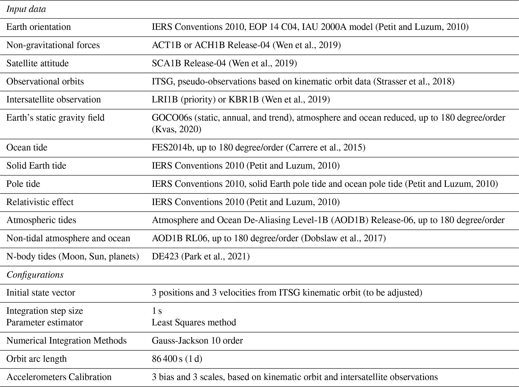
This section describes Step 1 as part of our LGD measurement processing shown in Fig. 1. This step aims to reduce the raw along-track observations (LRI1B and KBR1B) by removing most of the known gravitational and non-gravitational contributions unrelated to water mass changes. We make use of the open-source software Gravity and precisE ORBit determination system (GEORB; Papanikolaou, 2023) to integrate reference orbit, which is inferred by numerically integrating a series of gravitational potential models and non-gravitational measurements (see the details about input data in Table 1). The gravitational component includes the Earth's gravity, pole tide, solid Earth tide, and so on, all of which are provided by numerical models (e.g., Yuan, 2018). Here, we apply the Gravity Observation Combination of version 06s (i.e., GOCO06s; Kvas et al., 2021) gravity field model. The nonconservative forces, such as atmospheric drag and solar radiations, are derived from onboard accelerometer (ACT1B and ACH1B) and satellite attitude data (SCA1B) (Wen et al., 2019). A full compilation of the configuration for orbit integration is also provided in Table 1. In the orbit determination procedure, the arc length is set to one day and the a priori initial satellite state vector (position and velocity) is taken from the kinematic orbits provided by ITSG (Strasser et al., 2018). Six accelerometer calibration parameters (three biases and three scales) and initial state vector are adjusted by fitting the observational kinematic orbits and satellite-to-satellite tracking data (range-rate from KBR1B or LRI1B) simultaneously.

Figure 2 Analysis of range-rate and range-acceleration residuals on 18 July 2020. The top panel (a) shows KBR measurement residuals, and the bottom panel (b) shows LRI measurement residuals.

Table 1 Input data and configurations used for orbit integration in GEORB.

2.2 Generation of line-of-sight gravity difference

Based on the integrated reference orbit, we compute the intersatellite range-rate, defined as the projection of the relative velocity between the twin satellites onto the Line-Of-Sight (LOS) direction. By subtracting the modeled range-rate (derived from the reference orbit) from the measured range-rate (from KBR1B or LRI1B), we obtain the range-rate residuals. Taking the time derivative of these residuals yields the range-acceleration residuals. Figure 2 displays the time series of range-rate and range-acceleration residuals for an example day, 18 July 2020. It is evident that low-frequency components (e.g., their periodic patterns and amplitudes) of the range-rate residuals from both instruments (dark blue and red lines in Fig. 2) exhibit consistent patterns, indicating their comparable sensitivity at long-wavelength signals. In contrast, the range-acceleration residuals show clear discrepancies between the two sensors. The LRI range-acceleration residuals (light red line in Fig. 2b) demonstrate substantially lower noise than the KBR counterpart (light blue line in Fig. 2a) by virtue of smaller instrumental noise. The improved performance of the LRI indicates higher sensitivity to high-frequency residuals or short wavelength gravity changes.

When the twin satellites pass over regions with higher or lower than average surface mass distribution (i.e., the long-term mean), their gravitational accelerations are perturbed accordingly. The projection of intersatellite gravity difference onto the LOS direction is defined as LGD, i.e.,

$$\begin{array}{}\text{(1)}& \text{LGD}\left(t\right)=\left(\mathit{\delta }{\mathit{g}}_{\mathrm{1}}\right(t)-\mathit{\delta }{\mathit{g}}_{\mathrm{2}}(t\left)\right)\cdot {\mathit{e}}_{\mathrm{12}}\left(t\right),\end{array}$$

where δg₁(t) and δg₂(t) are the gravity vectors exerted by surface mass anomalies on the twin satellites at the given time t, and e₁₂(t) represents the LOS unit vector. Ghobadi-Far et al. (2018) have analyzed the spectra of LGD and range-acceleration residuals and reported high correlation and a constant admittance relationship between two time series at frequencies above 1 mHz. Thus, one can derive LGD from range-acceleration residuals using the following transformation:

$$\begin{array}{}\text{(2)}& \text{LGD}\left(t\right)={\mathrm{F}}^{-\mathrm{1}}\mathit{\left\{}Z\right(f)\cdot \mathrm{F}\mathit{\{}\mathit{\delta }\ddot{\mathit{\rho }}\left(t\right)\mathit{\left\}}\mathit{\right\}},\end{array}$$

where $\mathit{\delta }\ddot{\mathit{\rho }}\left(t\right)$ denotes the range-acceleration residuals as presented in Fig. 2, F and F⁻¹ represent the Fourier and inverse Fourier transforms, and Z(f) is the frequency-dependent transfer function defined as:

$$\begin{array}{}\text{(3)}& Z\left(f\right)=\mathrm{1.0}+{\mathrm{3.5}}^{-\mathrm{4}}{f}^{-\mathrm{1.04}},\end{array}$$

where f denotes the frequency variable. Finally, we obtain LGD variations with respect to the reference gravity model. Here, LGD is referenced only to the static component of GOCO06s so that the full time-varying gravity signal is preserved (see Sect. S1 in the Supplement for details). Note that the resulting LGD does not include signals below 1 mHz, since the spectral transformation is only performed at frequencies higher than 1 mHz. This treatment is necessary because the range-acceleration residuals contain contributions from both gravitational and centrifugal components. The transfer function accounts for the centrifugal acceleration term effectively only at the higher frequencies (>1 mHz, see Fig. 1 in Ghobadi-Far et al., 2018, for details).

2.3 L2- and climatology-based LGD

We also calculate two functional LGD time series, namely L2-based LGD and climatology-based LGD, which are synthetically computed using the L2 monthly mean gravity field solutions. The L2-based LGD synthetics serve two main purposes: (a) they enable comparison with the LGD measurements (KBR and LRI derived); and (b) they complement the LGD measurement time series by providing low-frequency gravity signals (<1 mHz) from the monthly mean LGD. The climatology-based LGD, in contrast, provides a reference baseline for identifying climatological “anomalies” in the LGD observations (hereafter, anomaly is defined as measurement minus climatological change). Based on the definition of LGD (Eq. 1), both functional LGDs can be derived from L2-based SH coefficients via spherical harmonic synthesis. For the detailed such procedure, readers can refer to Sect. 2.1 of Ghobadi-Far et al. (2018) and our open-source code (https://github.com/mTangcute/spherical-harmonic-synthesis, last access: 23 September 2025).

The L2 solutions are pre-processed to reflect accurate time-varying gravity signals. We first collect the SH data products with the maximum degree of 96 from the Center for Space Research (CSR) at the University of Texas at Austin (see details of these products in Sect. 6). Then, the degree-2 and degree-3 zonal coefficients are replaced with values derived from Satellite Laser Ranging (SLR) solutions (Loomis et al., 2020). To maintain consistency with the LGD measurements, the reference gravity field GOCO06s is removed from the L2 SH data products. These pre-processed SH coefficients are used to calculate the so-called L2-based LGD dataset. Note that in the synthesis procedure, only coefficients with degree less than and equal to 60 are included, which is equivalent to imposing a frequency cutoff of ∼10 mHz, corresponding to a 350 km spatial resolution. No further post-processing is required as the computation of LGD along the orbit at satellite altitude is an upward-continuation operation acting effectively as a smoothing filter often applied to L2 surface geopotential solutions.

The climatology-based LGD is computed from a set of climatological SH coefficients, which are derived from the pre-processed L2 SH time series. Specifically, L2 SH coefficient of each degree and order is fitted using the least squares with a model that includes a linear trend and a seasonal term (see Sect. S2 for details). Then, for a given date, the climatological SH coefficients are extracted from the fitted model across degree and order below 60, forming the input set for generating the climatology-based LGD. We use the SH solutions from 2003 to 2024 (a total of 22 years) to ensure a robust estimation of the climatological change in each of the coefficients (See also Sect. 3.2 of Tang et al., 2025b).

2.4 Spectral analysis in terms of LGD

As shown in Fig. 3, we analyze the amplitude spectral density (ASD) of LGD to evaluate signals and noises from the different ranging instruments. The sampling intervals are 5 s for KBR and 2 s for LRI, corresponding to Nyquist frequencies of 100 and 250 mHz, respectively. As such, the derived LGD signals span 1–100 mHz for KBR (blue curve) and 1–250 mHz for LRI (red curve). KBR-based LGD measurements are dominated by instrumental noise at frequencies above 10 mHz, manifesting as the increasing spectral density. In contrast, LRI retains its sensitivity to the signal at a broader frequency range up to ∼20 mHz, which is consistent with the LRI cutoff frequency reported by Peidou et al. (2022). As a result, in this study, we apply a 6th-order Butterworth bandpass filter to preserve signals up to 10 mHz for KBR and up to 20 mHz for LRI, as shown by the purple and yellow curves. Note that the gradual attenuation observed in the bandpass filtered KBR-LGD spectrum (purple curve) within the 10–20 mHz spectral band reflects the filter's roll-off characteristics rather than actual signals. Additionally, we present the ASD of L2-LGD, which shows a good agreement with both KBR-LGD and LRI-LGD within the 1–10 mHz spectral band and drops sharply beyond 10 mHz as L2 data have been truncated at degree 60. The KBR and LRI derived LGD datasets are available only from 1 mHz, and thus we augment these LGD measurements by adding the L2-LGD but only at the frequencies below 1 mHz. Therefore, the fully reconstructed LGD time series refer to monthly mean gravity at the frequency less than 1 mHz (approximately equivalent to SH degree lower than 6) and instantaneous gravity at frequency higher than 1 mHz (SH degrees higher than 6).

Figure 3 Amplitude spectral density of LGD time series on 18 July 2020. Blue and red curves represent LGD spectra derived from KBR and LRI observations, respectively. Green curve corresponds to LGD synthesized from L2 SH solutions. Purple and yellow curves show band-pass filtered LGD from KBR and LRI, with cutoff frequencies of 10 and 20 mHz, respectively. Vertical dashed lines indicate the 10 and 20 mHz thresholds used for filtering.

Above analyses support the possible strategies for processing LGD data across different frequency bands. As shown by the dashed arrows and lines in Fig. 1, band-pass filters should be applied to KBR-LGD and LRI-LGD to suppress instrument noise, while the low-frequency components (<1 mHz) from the L2-based LGD can be incorporated when a full-spectrum gravity change signal is sought after (see Sect. S3 for details of the frequency-domain processing and spectral combination).

3 Dataset description

3.1 Data structure and availability

As presented in Fig. 4a, the LGD dataset is divided into two subsets according to the different ranging instruments (KBR and LRI). Each subset is organized by date, spanning June 2018 to December 2024. Daily files (e.g., lgd20200718, Fig. 4b) provide instantaneous LGD measurements sampled along the GRACE-FO satellite trajectories. The data are stored in plain text, where each row represents an observation at 5 s intervals for KBR or 2 s intervals for LRI, and includes the following variables:

• Variable 1: observation time, expressed as GPS time in continuous seconds since 1 January 2000 11:59:47 UTC

• Variables 2–4: longitude, latitude, and altitude of the twin satellites' midpoint at that epoch

• Variable 5: LGD_full, representing the unfiltered, full-spectrum LGD value

• Variable 6: LGD_band, containing LGD signals retained after bandpass filtering (e.g., <10 mHz for KBR and <20 mHz for LRI; hereafter, KBR-based LGD_band and LRI-based LGD_band results are denoted as KBR-LGD and LRI-LGD, respectively)

• Variable 7: LGD_low, representing LGD signals below 1 mHz, which is extracted from L2-synthesized LGD

• Variable 8: LGD_L2, the synthetic LGD from L2 SH coefficients up to 60, limited to the frequency band below 10 mHz

• Variable 9: LGD_clm, LGD climatology, which is the synthetic LGD from the climatological estimates of the SH coefficients

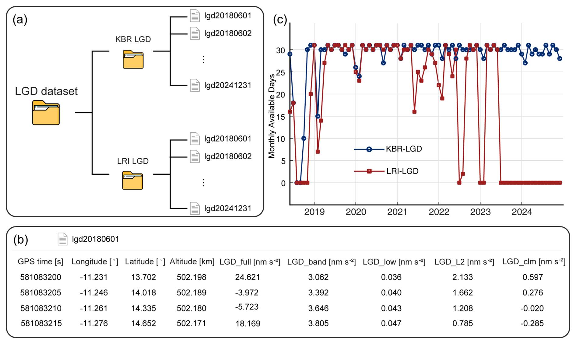
Figure 4 Structure and availability of the dataset. (a) Daily files are organized by date, each containing measured LGD and functional LGD sampled along GRACE-FO satellite orbits. (b) Example of file contents, including observation time, geodetic coordinates, and LGD products: LGD_full, LGD_band, LGD_low, LGD_L2, and LGD_clm (See the main text for each of these LGD dataset). Units of all LGD-related variables are nm s⁻². (c) Data availability from KBR and LRI instruments.

We count the number of available days month by month. As shown in Fig. 4c, the experimental LRI exhibits more frequent data gaps in comparison to KBR. Most missing days in both datasets are attributed to the unavailability of essential L1B data files, such as intersatellite ranging measurements or non-gravitational force observations. Another cause, to a much smaller extent, is the instability of reference orbit integration, which may arise from factors such as accelerometer parameter estimation and the quality of the observational orbits. For LRI system, moreover, the satellite attitude control adopted a wide deadband pointing mode after July 2023 (Landerer et al., 2020). This mode did not meet the precision requirements for scientific observation, resulting in a prolonged LRI outage.

3.2 Examples and interpretation of LGD data

We now present an example of LGD dataset along one selected track (highlighted in red in Fig. 5a) on 18 July 2020 to illustrate the components of our dataset in detail. Figure 5b shows different functional LGDs, while Fig. 5c displays LGD components encompassing different frequency bands. It is important to note that the magnitude of LGD variations is tied to how much the surface mass (or gravity) changes, but their signs are reversed, that is, a positive surface mass (or gravity) change features a negative LGD variation (see Fig. 1 in Tang et al., 2025). All these LGD results in Fig. 5 represent the gravity change with respect to the static component of GOCO06s.

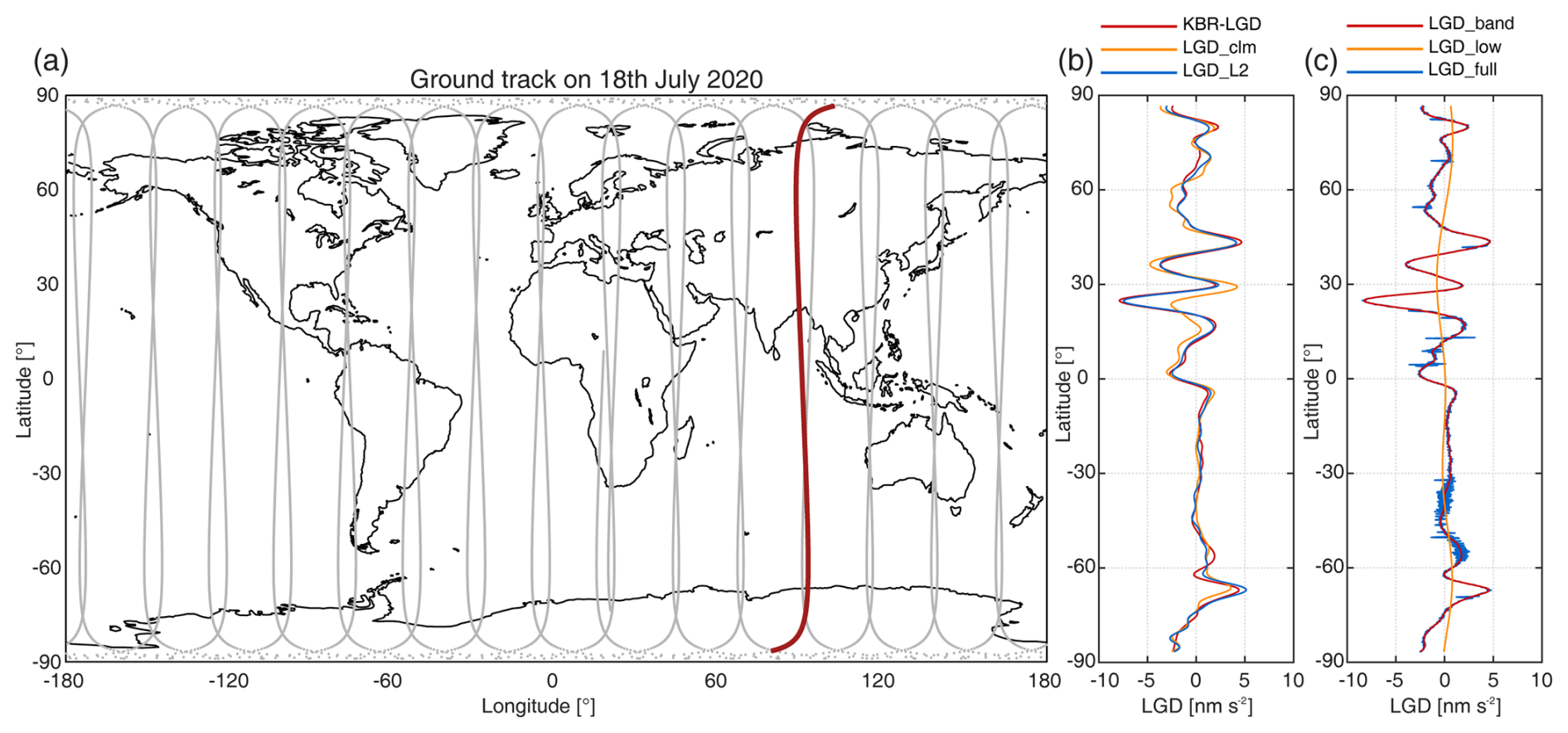
Figure 5 Examples of LGD data. (a) GRACE-FO ground tracks on 18 July 2020, with the red curve marking one ascending orbit selected for demonstration. Gray curves denote other satellite passes on the same day. (b) LGD values along the selected track in (a). The red, blue, and orange curves correspond to KBR-LGD, L2-based LGD, and climatology-based LGD, respectively (all from the KBR dataset). (c) LGD from the LRI dataset, with blue, red, and orange curves representing full-spectrum, band-pass filtered, and low-frequency components, respectively.

As shown by the along-track KBR-LGD (red curve) in Fig. 5b, the GRACE-FO spacecraft passed over several regions with significant hydrological mass changes, particularly near 25° N (LGD change of −8 nm s⁻²) and 70° S (LGD change of +5 nm s⁻²). The LGD synthesized from L2 SH coefficients (LGD_L2; blue curve) closely matches the KBR-LGD measurements. The difference arises because KBR-LGD reflects instantaneous along-track gravity changes, whereas LGD_L2 is synthesized from monthly averaged gravity fields. Consequently, LGD_L2 cannot resolve intra-month gravity variations that are preserved in the KBR-LGD measurements. For example, over East Antarctica (around 70° S in Fig. 5b), the discrepancy between LGD_L2 and KBR-LGD reaches about 0.5 nm s⁻², indicating that the monthly L2 solutions could overestimate the magnitude of short-term water mass changes.

In contrast, the climatological LGD (LGD_clm; orange curve shown in Fig. 5b) represents the LGD synthesized from the climatological fit of the L2 spherical harmonic solutions for July 2020. The gravity difference between the measured KBR-LGD and LGD_clm indicates the deviation from climatology, and thus referred to as the climatological anomaly (Thomas et al., 2014). Such anomalies are typically associated with hydrological extremes like floods or droughts. For example, the strong negative LGD observed near 25° N suggests an anomalous increase in water mass, which results from a wet extreme event (Han et al., 2021a).

Figure 5c presents LGD examples from the LRI dataset across different frequency bands. The full-spectrum LGD (blue curve) includes all spectra available in the measurement bandwidth (0–250 mHz), while the bandpass-filtered LGD (red curve) retains signals below 20 mHz. The difference between the two is associated with high-frequency components within the 20–250 mHz spectra. Spikes observed near the equator are likely due to non-gravitational accelerations associated with thrust firing events that were not removed from the onboard accelerometers processing (Wen et al., 2019). High-frequency oscillations between 30 and 60° S arise likely from LRI instrument noise or errors in the Atmosphere and Ocean De-aliasing (AOD) model (Shihora et al., 2022). The low-frequency components (<1 mHz; orange curve), computed from the L2 gravity solutions (i.e., not derived from L1B data), contain long-wavelength gravity signals (half-wavelengths of 3500 km or longer). Their variance is approximately 7 % of that of the bandpass-filtered LGD (i.e., yellow vs. red curves in Fig. 5c), indicating that the low-frequency component contributes only a small fraction of the overall LGD variability.

3.3 Global demonstration of LGD

We put all available LGD measurements throughout July 2020 together to generate a map of global water mass variations. The resulting KBR-LGD and LRI-LGD maps (Fig. 6a and b) are highly consistent, despite being band-pass filtered with different cutoff frequencies (10 mHz for KBR-LGD and 20 mHz for LRI-LGD). In principle, LRI-LGD features additional gravity signals over 10–20 mHz (Fig. S2), in our LGD data products. For example, Peidou et al. (2022) demonstrated that, in the 15.6–31.2 mHz waveband, LRI exhibits superior sensitivity to high-amplitude signals in regions such as Greenland and Antarctica.

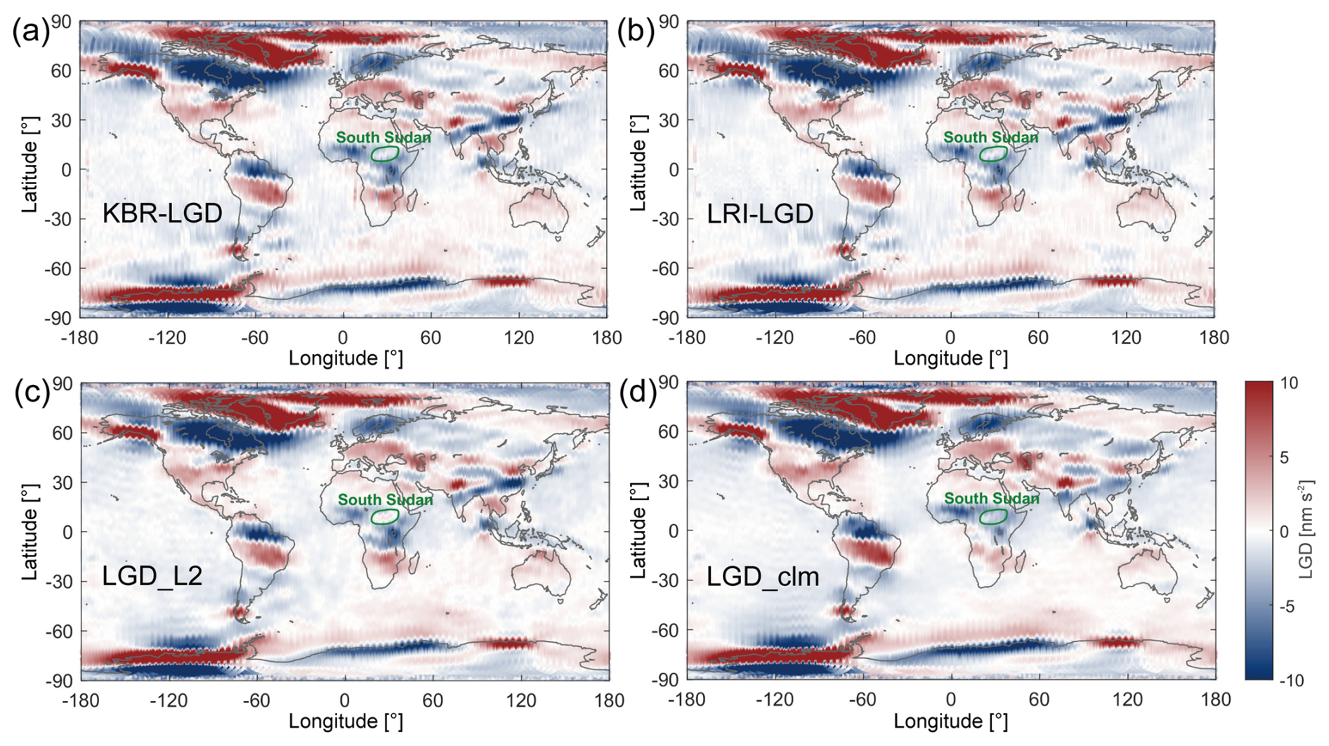
Figure 6 Global maps of LGD and water mass changes for July 2020. Panels (a)–(d) show LGD derived from KBR, LRI, L2 data, and climatology, respectively. Note that KBR-LGD, LRI-LGD, LGD_L2, and LGD_clm contain signals with frequencies below 20, 10, 10, and 10 mHz, respectively.

For comparison, the global map derived from LGD_L2 is presented in Fig. 6c. While the measured and L2-synthetic LGD fields agree well overall (Fig. 6), several discrepancies are evident. For example, one notable mismatch occurs over South Sudan (circled in green in Fig. 6). This suggests that South Sudan potentially experienced intra-month hydrological dynamics that cannot be resolved by monthly LGD_L2. Figure 6d shows the LGD_clm map for this month, which differs even more markedly from the other panels (Fig. 6a–c). Note that these differences reflect anomalous events (e.g., droughts and floods) rather than intra-month mass variations. The applications of the LGD-based climatology will be described in detail in Sect. 4.

We now demonstrate an example of sub-monthly gravity change observation from KBR and LRI derived LGD data in contrast to L2 synthetics. Figure 7 presents the LRI-LGD and LGD_L2 results for July 2020 with a 10 d interval. Several regions including South Sudan mentioned in Fig. 6 exhibit obvious intra-month changes (indicated by the purple rectangles in Fig. 7a–c). For instance, SouthEastern United States (SEUS, region #1) and the Amazon basin (region #2) display LGD increases (i.e., TWS decreases), whereas western Africa, South Sudan, Bangladesh, and the Yangtze River basin (regions #3, #4, #5, and #6) show the opposite trends. Notably, northern Russia (region #7) shows more dynamic patterns with LGD first decreasing and then increasing even within a month.

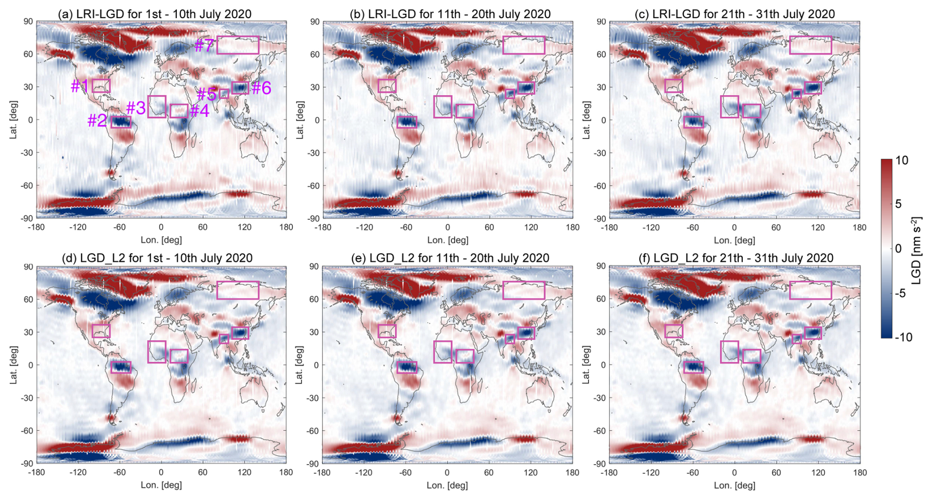
Figure 7 Global LGD maps at a 10 d interval during July 2020. The top row (panels a–c) shows LRI-LGD results, and the bottom row (panels d–f) shows LGD_L2 results. Each column corresponds to early, mid, and late July, respectively. In panel (a), purple rectangles mark regions with evident intra-month variations. Regions #1–#7 correspond the southeastern United States, Amazon basin, western Africa, South Sudan, Bangladesh, Yangtze River basin, and northern Russia.

In contrast, LGD_L2 results for early, mid, and late July remain constant (Fig. 7d–f), lacking these intra-month variations. Taking region #2 as an example, we calculate the average of all LGD observations within the rectangle. The LRI-LGD changes by 1.5 nm s⁻² from early July (−13 nm s⁻²) to mid-July (−11.5 nm s⁻²), but then increases by 3 nm s⁻² from mid to late July (−11.5 to −8.5 nm s⁻²). Such non-uniform intra-month changes even cannot be reproduced by any means of monthly solutions. The intra-month reversal behavior in region #7 is not observed by the monthly L2 gravity solutions. These examples provide preliminary evidence for key advantages of our LGD data products in resolving sub-monthly hydrological variabilities.

3.4 Capability of LGD measurements for tracking water mass changes at sub-monthly scales

We demonstrate the LGD measurements for tracking water mass changes at the sub-monthly scale from both long-term monitoring and short-term event perspectives. To evaluate long-term variability, global LGD maps with a 10 d interval as showed in Fig. 7 are used to calculate zonally averaged LGD time series across 45° S–45° N throughout 2020. The resulting LRI-LGD maps (Fig. 8a) show a continuous evolution of gravity change over time, with intra-month fluctuations (differences between early, mid, and late parts of each month) clearly visible across most latitudes. In contrast, the monthly LGD_L2 products feature discrete monthly-mean patterns (Fig. 8b). The significant seasonal variation occurs within ±20° of the equators, where both hemispheres display the pattern of water gains during local summer and losses during winter. Figure 8c illustrates LGD time series at 5° N, the equator, and 5° S, showing that our LGD data products capture more details of water mass changes than the monthly L2 data products.

Figure 8 Zonally averaged LGD time series across 45° S–45° N for 2020, derived from the global LGD maps at a 10 d interval shown in Fig. 7. Panels (a) and (b) present results from LRI-LGD and LGD_L2, respectively. Horizontal lines indicate the selected latitudes for which the LGD time series are presented in panel (c). In panel (c), dark lines represent LGD_L2 time series, and light lines represent LRI-LGD time series.

Building on these insights from the zonally averaged time series, we examine specific short-term events to evaluate the advantage of LGD measurements. We focus on the rapid hydrological dynamics occurring over the central Amazon basin and South Sudan during July–August 2020. A 4°×4° study area is first defined (gray boxes in Fig. 9a and d), and regional water mass changes are assessed using along-track LGD measurements crossing this region (colored lines in Fig. 9a and d). The corresponding LRI-LGD and LGD_L2 results along the orbital trajectory are displayed in Fig. 9b and e. To demonstrate a more intuitive temporal dynamic of hydrological variations, we apply a weighted averaging (Sect. S4) of the along-track LGD time series to derive the time-varying LGD over the target regions (Fig. 9c and f). The weights follow a Gaussian distribution as a function of the latitudinal distance between each observation point and the block center, with a standard deviation of 200 km.

Figure 9 Along-track LGD revealing hydrological changes in the Amazon and South Sudan during July–August 2020. Panels (a) and (d): geographic locations of the Amazon and South Sudan. Black lines show coastlines, gray boxes mark each study region, and colored lines denote GRACE-FO ground tracks passing through the regions. Panels (b) and (e): along-track LGD crossing the study areas on different dates. Colored curves represent LRI-LGD and black curves denote LGD_L2. Two horizontal dashed lines show the latitude bounds of each study region. For clarity, LGD curves in panels (b) and (e) are shifted by 10 and 5 nm s⁻², respectively. Gray arrows highlight discrepancies between LRI-LGD and LGD_L2. Panels (c) and (f): Time series comparisons of LRI-LGD (colored bars) and LGD_L2 (gray bars) for two study areas during July–August 2020. These time series are derived through weighted averaging (see text) LGD within the region.

In the Amazon basin (Fig. 9b and c), both LGD measurements and L2 synthetics reveal a substantial increase over July–August. The LRI-LGD shows continuous increase (i.e., water mass depletion) with the value increasing from −13.9 to +1.3 nm s⁻², whereas the LGD_L2 exhibits step-like month-to-month variations. For example, from 27 July to 1 August, the LRI-LGD increases moderately from −9.5 to −6.5 nm s⁻², while the L2-LGD jumps sharply from −12.0 to approximately −2.0 nm s⁻² due to its monthly resolution. This comparison highlights that LGD is an instantaneous measurement that can provide accurate information on the timing and magnitude of water mass changes. As indicated by the gray arrows in Fig. 9b, the monthly mean LGD_L2 underestimates water mass change in early August (1 and 7 August) and overestimates it in late August (23 and 29 August).

In South Sudan (Fig. 9e and f), LGD measurements show a transition from water losses (LGD>0) to water gains (LGD<0) between July and August, decreasing from +2.3 to −4.4 nm s⁻². Discrepancies between LRI-LGD and LGD_L2 are also evident here: LGD_L2 underestimates the water mass changes on 4 and 10 July, and 1 and 6 August (indicated as the right arrows in Fig. 9e) and overestimates them on 26 July and 28 August (indicated as the left arrows in Fig. 9e). We observe that the magnitudes of LGD_L2 varies throughout July (Fig. 9f), which is attributed to the changing orbit during each satellite overpass of the region (Fig. 9d). These critical intra-month variations are discerned in LGD measurements because each region is revisited multiple times per month, typically every 5–6 d in most low and mid latitude regions (depending on latitude). In both the Amazon and South Sudan, having 5–6 LGD observations per month provides detailed temporal dynamics that are lost when using monthly mean products.

4 Applications in terms of hydrological extreme characterization

The instantaneous and observational nature of the LGD enables precise estimation of water mass dynamics at a finer scale than a month. It is therefore a straightforward application of this new dataset to characterize sub-monthly hydrological extremes. In addition to releasing LGD measurements, we also provide a climatological gravity change model in the form of along-track LGD (i.e., LGD_clm), which allows identification of anomalies deviating from the climatological norm. We demonstrate how the LGD dataset, comprising both measurements and climatology, can be used for (1) near real-time monitoring of rapid hydrological extremes and for (2) evaluating long-term hydrological extremes in hotspot regions.

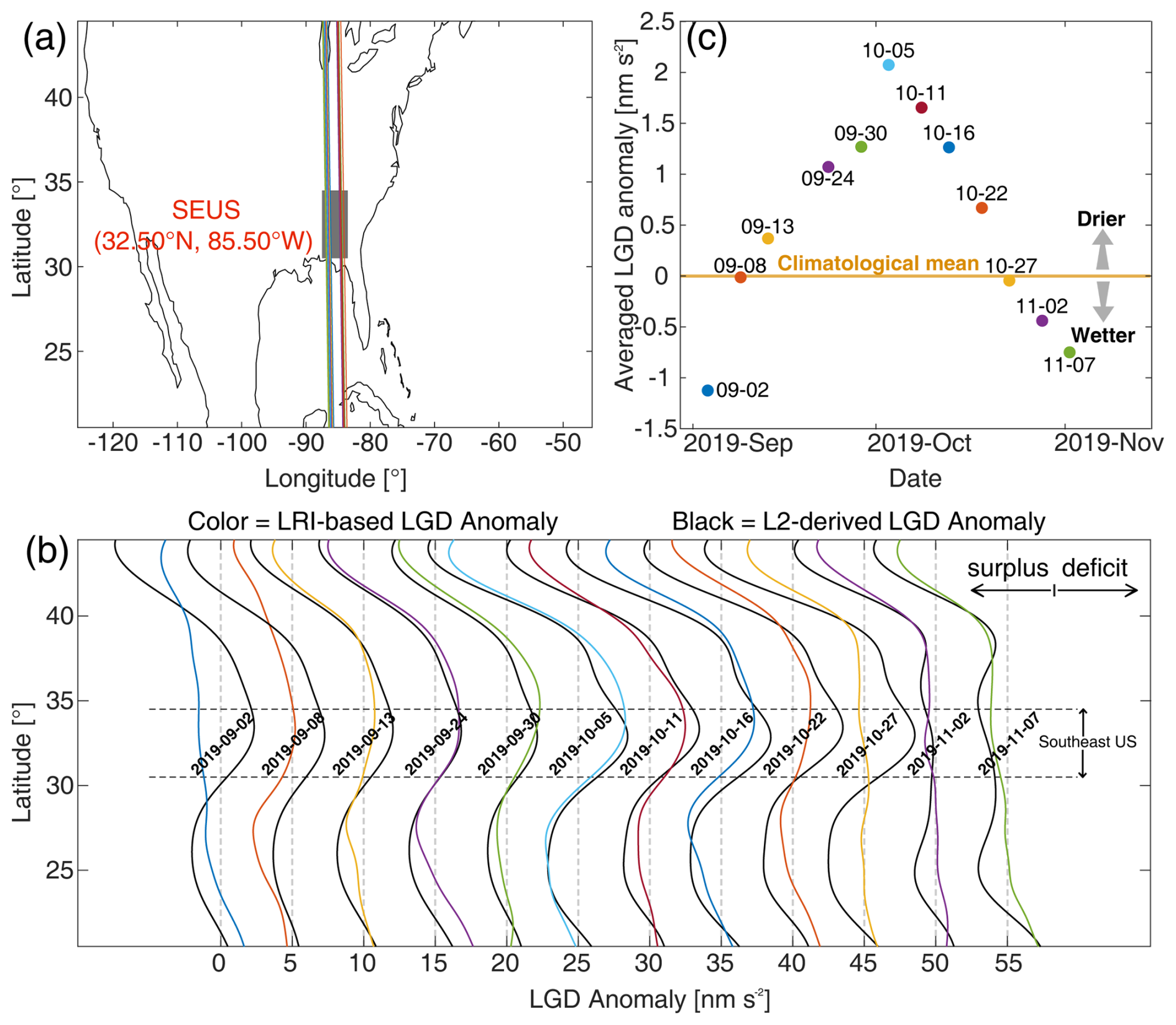
Figure 10 LGD analysis of the flash drought event in the SEUS from September to November 2019. (a) Study region (gray box) centered at 32.5° N, 85.5° W. Colored lines represent GRACE-FO ground tracks intersecting the region during September–early November. (b) Along-track LGD anomalies for each satellite pass, with colored lines denoting LRI-based anomalies (LRI-LGD minus climatological LGD) and black lines showing L2-derived anomalies (LGD_L2 minus climatological LGD) for comparison. Negative LGD anomalies indicate wetter-than-normal conditions, while positive anomalies indicate drier-than-normal conditions. (c) Averaged LGD anomalies over the SEUS through weighted averaging.

4.1 Monitoring of rapid hydrological extremes

Rapid hydrological extreme events may evolve at sub-monthly timescales. For instance, floods occur as dynamic phenomena over days to weeks (Najibi and Devineni, 2018), and flash droughts can intensify and recede within a few weeks (Otkin et al., 2018; Yuan et al., 2023). However, GRACE-FO L2 and L3 products are limited by their (a) monthly resolution and (b) latency of a few months, making them unsuitable for timely monitoring and early warning of such extremes (Landerer et al., 2020). The developed LGD dataset addresses the first limitation by resolving along-track information on instantaneous water mass changes. In addition, the latency issue can be alleviated by utilizing low-latency (1–3 d) Quick-look L1B data (Wen et al., 2019; Kvas, 2020). In our previous work, we have demonstrated that LGD based on Quick-look L1B data can track rapid flood events in eastern Australia and quantify the associated water mass increase in near real-time (Han et al., 2021b).

We now incorporate the along-track GRACE climatology to assess whether such water mass changes lead to abnormally wet or dry conditions. We showcase the SEUS (Fig. 10a) as an example to demonstrate monitoring of a flash drought. Likewise, only the along-track LGD measurements from satellite passes whose ground tracks intersect the study region are examined. By subtracting the climatological LGD from the LGD measurements, we derive the along-track LGD anomalies (i.e., deviation from typical hydrological conditions) over SEUS during September to early November 2019 (Fig. 10b). The LGD anomaly time series for the SEUS (Fig. 10c) is derived from along-track LGD anomalies using the same weighted averaging method as that applied in Fig. 9c and f.

The results show that, at the beginning of September, the LGD anomaly indicated wetter than normal conditions (−1.2 nm s⁻² on 2 September). By 8 September, conditions had dried to near normal before rapidly transitioning to water deficit. The drought intensified and peaked on 5 October, when the LGD anomaly reached +2.2 nm s⁻², and then gradually receded, recovering to normal conditions by 27 October. By early November, SEUS had returned to conditions as wet as early September. National Oceanic and Atmospheric Administration (NOAA) reported this flash drought event using US Drought Monitor (USDM) dataset, which is consistent with our results. They attributed it to the record-breaking heat and the absence of tropical rains across the broader region (NOAA, 2019). Compared to the L2-based LGD anomalies, the LRI- and KBR-based LGD anomalies provide obvious advantages in both diagnosing hydrological anomalies and resolving their temporal characteristics. Specifically, the L2-based LGD anomalies misidentify that SEUS was already dry in early September, while the LRI-LGD anomalies show it was still wetter than normal. Moreover, the L2 results consistently overestimate the severity of dryness throughout September and October. In contrast, the LGD dataset accurately detects the onset (8 September), peak (5 October), and termination (27 October) timings of this flash event, which cannot be resolved from monthly L2 products. Operationally, once GRACE-FO spacecraft overpass the study area and L1B data become available, LGD anomalies can be directly derived to capture flash extremes in near real-time and, importantly, to provide early warning based on the evolution of such events.

4.2 Standardisation of gravity anomalies

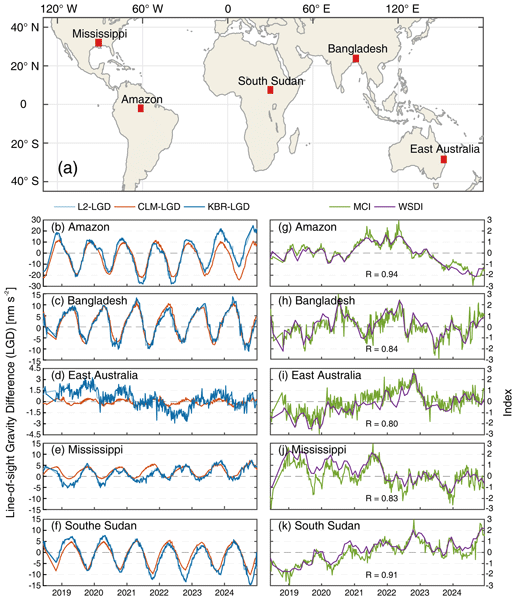
The LGD data products provided from this study can also be used to detect and quantify anomalous events. Tang et al. (2025) developed a method to standardize the LGD time series to obtain the hydrological index based on gravity anomaly (relative to the climatological mean field) and demonstrated dynamic hydrological extreme events along the Yangtze River. The standardization converts the gravity anomaly data to dimensionless indices, Mass Change Index (MCI), by introducing the statistical distribution functions. The methodology starts with dividing the study area into 4°×4° blocks (e.g., red boxes in Fig. 11a). For each block, we construct two time series: one from LGD measurements and the other from the LGD climatology (dark blue and orange lines in Fig. 11b–f). These regional time series are derived using the same method as the results shown in Fig. 10c. Taking their difference yields the LGD anomaly time series. Finally, these anomalies are standardized to produce the MCI (see the details in Tang et al., 2025).

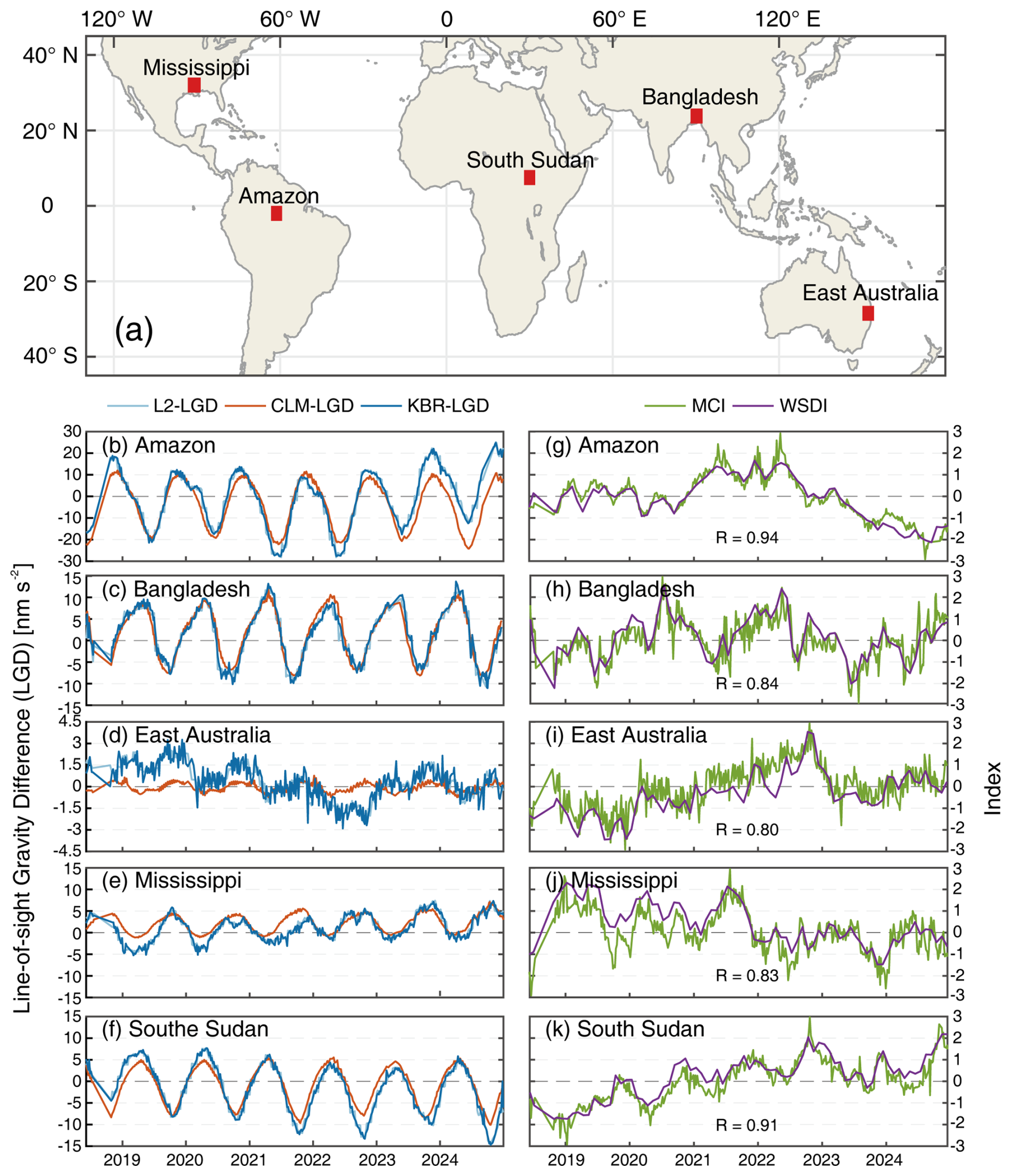
Figure 11 Identification and characterization of sub-monthly hydrological extremes in global hotspot regions during the GRACE-FO period using the Mass Change Index (MCI). (a) Locations of the five hotspot regions (red boxes): Mississippi, Amazon, South Sudan, Bangladesh, and eastern Australia. (b–f) Regional LGD time series, including measured LGD (dark blue lines), synthetic LGD_L2 (light blue lines), and climatology-based LGD (orange lines). Note that panels (b) and (d) use a different y axis scale. (g–k) Comparison of the MCI (green lines) with the Water Storage Deficit Index (WSDI; purple lines) derived from monthly L2-derived TWS. Correlation coefficients (R) between WSDI and MCI are given in each panel.

We present results for five hotspot regions (Amazon, Bangladesh, eastern Australia, Mississippi, and South Sudan; Fig. 11a) to demonstrate the use of LGD measurements to capture sub-monthly hydrological extremes worldwide. As shown in Fig. 11b–f, the behaviours of L2- and L1B-based LGD are consistent with the findings in Fig. 8c, where the LGD measurements capture intra-month variations that are otherwise not found from the monthly L2 products. Eastern Australia differs from the other four areas (Fig. 11d), with the LGD time series showing the strongest short-term fluctuations. These fluctuations, quantified as the Root Mean Square (RMS) of the difference between KBR-LGD and L2-based LGD relative to the RMS of the KBR-LGD signal, reach approximately 46 %, compared with 23 %, 14 %, 15 %, and 19 % for the Mississippi, Amazon, South Sudan, and Bangladesh, respectively. This is likely attributed to the relatively small magnitude (approximately ±3 nm s⁻²) of water mass changes in Eastern Australia makes the signal more susceptible to leakage from surrounding areas. Notably, similar wiggles appear in the LGD climatology time series because the same weighted averaging is applied. Thus, when computing LGD anomaly time series, these leakage and orbit-related artifacts are partially cancelled, resulting in more reliable anomaly signals.

Figure 11g–k present the MCI results derived from the standardized LGD anomalies. For comparison, we also derive water storage deficit index (WSDI) following the same methodology but with monthly L2-derived TWS estimates (see the methodology in Sun et al., 2018). MCI exhibits short-term variabilities likely originated from sub-monthly hydrological extremes and LGD or model errors, each of which needs to be validated. Our previous study (Tang et al., 2025) extensively validated and demonstrated that, in the Yangtze River basin, these short-term anomalies are indeed caused by hydrological extremes. It is important to note that L2-LGD is synthesized from monthly L2 gravity fields and therefore represents only the monthly mean state, rather than true sub-monthly variability. The MCI is a new type of hydrological index detecting and characterizing water storage anomalies at shorter time scales than traditional monthly index (e.g., WSDI), potentially offering substantial advantages to operational monitoring of sub-monthly hydrological extremes.

5 Uncertainty, usage, and recommendations

5.1 Uncertainty of the LGD measurements

We evaluate the uncertainty in LGD measurements from two primary sources: (1) instrument noise of the KBR and LRI ranging systems, and (2) errors in the background models propagated through reference orbit integration. Figure 12 shows the ASD of LGD time series derived from measurements, instrument noise, and background model errors. The nominal range noise of KBR is 1 $\mathrm{\mu }\mathrm{m}{\mathrm{Hz}}^{-\mathrm{1}/\mathrm{2}}$ (Kim, 2000), and when propagated into LGD, it appears as a noise spectrum that increases with frequency (green curve). The spectra of KBR-LGD measurements (blue curve) shows the actual KBR noise less than the nominal ranging noise roughly by a factor 2 at 20 mHz. On the contrary, the theoretical LRI noise spectrum (yellow curve) (Abich et al., 2019) is smaller than the actual LRI performance (red curve). The LRI sensitivity seems extended up to around 20 mHz from which the LRI noise becomes dominant. Given that the nominal noise models do not adequately reproduce the noise-dominated portions of the observed spectra, we additionally fit empirical power-law models to the high-frequency spectra. The fitted KBR-LGD and LRI-LGD noise models are: $\text{ASD}(f{)}_{\text{KBR-LGD}}^{\text{noise}}=\mathrm{3332}{f}^{\mathrm{1.5}}$ (f>10 mHz) and $\text{ASD}(f{)}_{\text{LRI-LGD}}^{\text{noise}}=\mathrm{1.2}{f}^{\mathrm{0.17}}$ (f>20 mHz), respectively. The low-frequency (i.e., <10 mHz for KBR and <20 mHz for LRI) sensor-noise model is not estimated because the low-frequency spectrum is not dominated by instrument noise alone, but primarily reflects geophysical signals, with background-model errors contributing to a lesser extent.

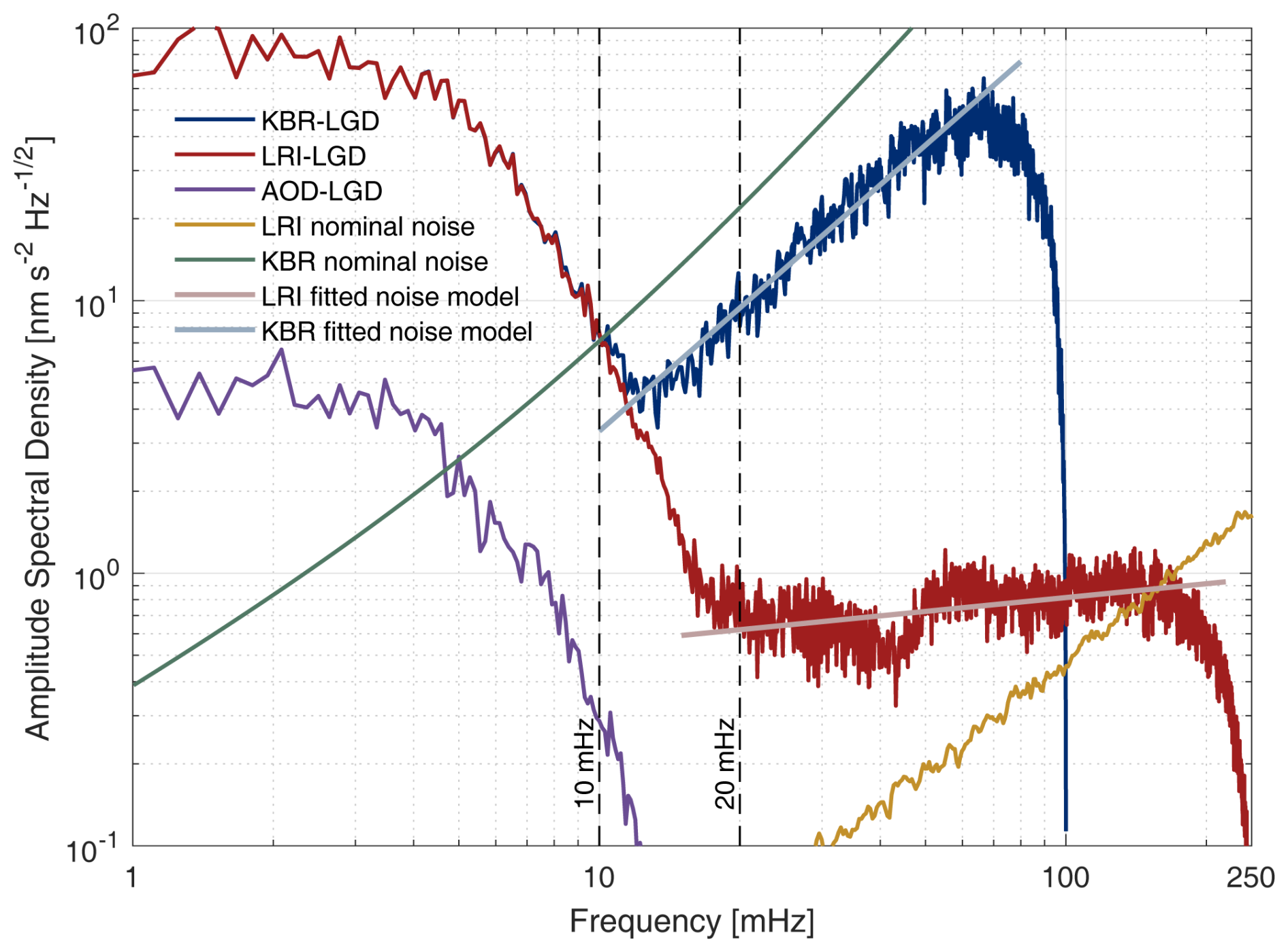
Figure 12 Amplitude spectral density of intersatellite ranging measurements, instrument noise, and background model errors, all expressed in terms of line-of-sight gravity differences. Green and yellow curves denote the nominal instrument noise from the KBR and LRI ranging systems, respectively. Blue and red curves show the spectra of KBR-LGD and LRI-LGD measurements. The purple curve represents errors associated with background model differences (AOD1B RL07 vs. RL06). The light blue and light red curves show the empirical power-law fits to the high-frequency (noise-dominated) portions of the KBR-LGD and LRI-LGD spectra, respectively. Vertical dashed lines at 10 and 20 mHz indicate the cutoff frequencies used for KBR-LGD and LRI-LGD filtering, respectively.

Taking the datasets on 18 July 2020 as an example, we compute band-limited RMS (i.e., $\sqrt{{\int }_{f_{\mathrm{1}}}^{f_{\mathrm{2}}}\text{ASD}(f{)}^{\mathrm{2}}\mathrm{d}f}$, where f₁ and f₂ define the lower and upper bounds of the measurement frequency band) to quantify signal and instrument noise level. For KBR-LGD, the RMS is ∼5.0 nm s⁻² within the 1–10 mHz band, while it reaches 9.5 nm s⁻² in the instrument noise-dominated 10–100 mHz band. In contrast, LRI-LGD shows improved performance: the RMS within the 1–20 mHz (signal) band is also ∼5.0 nm s⁻², while the RMS over (noise-dominated) 20–250 mHz is substantially reduced to 0.4 nm s⁻². Therefore, in our released dataset, we recommend using the band-pass filtered LGD (the sixth column, LGD_band, in each LGD file) for surface mass change applications.

Error in the background models (e.g., static gravity models, tidal models, and non-tidal atmosphere and ocean models) can propagate into LGD through reference dynamic orbits. These errors are generally larger than the instrument noises and may be at the same order of magnitude as the signals of interest. For example, Han et al. (2020) analyzed the impact of tidal model errors (FES2014b vs. GOT4.7) and found that M2 tide induced gravity disturbances can reach ∼1 nm s⁻² in some coastal areas (see Fig. 7 in Han et al., 2020, and Fig. S3). Ghobadi-Far et al. (2020b) demonstrated that adopting GOCO06s as the static gravity field yields smaller error with RMS<0.2 nm s⁻² in the 17–35 mHz frequency band, whereas the other model such as GGM05C produces RMS values as large as 5 nm s⁻² (see Fig. 4 in Ghobadi-Far et al., 2020b). In this study, we examine the impact of non-tidal model errors using two state-of-the-art AOD models: AOD1B RL07 (Shihora et al., 2022) and its RL06 (Dobslaw et al., 2017). The spectrum of LGD residuals between two AOD models (purple curve in Fig. 12) reveals significant error, particularly at frequencies <4 mHz, with ASD reaching 5 $\mathrm{nm}{\mathrm{s}}^{-\mathrm{2}}{\mathrm{Hz}}^{-\mathrm{1}/\mathrm{2}}$ that is higher than the expected KBR and LRI instrument noises. The band-limited RMS of their difference within 1–10 mHz frequency band is ∼0.3 nm s⁻², about an order of magnitude smaller than the signal RMS. However, this represents only a lower bound of the true uncertainty, since the two AOD models are not independent. Actual errors are likely larger, as demonstrated by the tidal model case (Han et al., 2020). In summary, the LGD error from the instrument noise is insignificant over the signal band width (1–20 mHz) but its magnitude exceeds that of the signals rapidly from 10–20 mHz. The mis-modelled systematic geophysical signals, such as unmodeled or mismodeled tides, are far more significant and may be as large as ∼1 nm s⁻².

5.2 Usage and recommendations

The demonstrations shown in this study highlight the value of the LGD dataset for monitoring short-term TWS variability as well as quantifying long-term hydrological anomalies at the sub-monthly scale. Beyond these applications, LGD have proven broader utility: earlier studies applied LGD to investigate ocean tides (Han et al., 2020), tsunamis (Ghobadi-Far et al., 2020a), and reservoir operations (Yi et al., 2025), while more recent work has shown that along-track LRI measurements are sensitive enough to detect atmospheric water mass variations (Kracheletz et al., 2025), which implies that LRI-LGD probably can also discern these changes. In addition, LGD provides valuable constraints for calibrating or validating hydrological and geophysical models. For example, the benefits of assimilating LGD instantaneous gravity change data into a land surface model have been demonstrated in comparison to assimilating monthly gravity data (Khaki et al., 2023). Han et al. (2021a) used LGD to constrain effective flood wave velocities along river channels and floodplains, and Ghobadi-Far et al. (2020b) employed LGD to demonstrate the superior performance of the GOCO06s static gravity model. All applications underscore the substantial potential of instantaneous LGD measurements for advancing Earth system science.

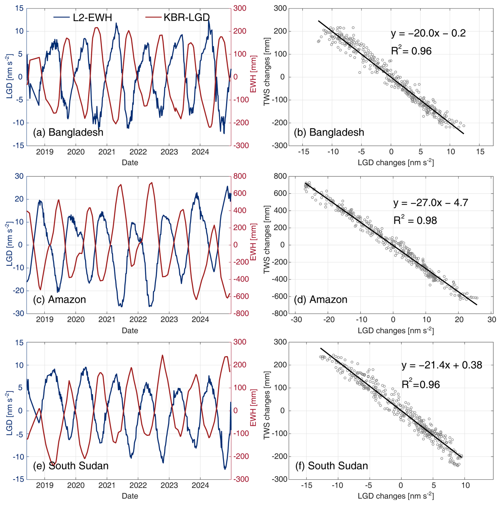
Figure 13 Comparisons between LGD variations and L2-based EWH time series in Bangladesh, Amazon, and South Sudan. The first column shows the time series of KBR-LGD (red lines) and L2-derived EWH (blue lines) from June 2018 to December 2024 in Bangladesh (a), Amazon (c), and South Sudan (e). The second column presents the linear regressions between LGD and EWH, where gray dots represent individual samples and black lines denote the fitted regression lines. Note that these scatter points are obtained by resampling the EWH time series to match the LGD sampling intervals. The fitted slopes indicate that a 1 nm s⁻² change in LGD corresponds to approximately −20.0, −27.0, and −21.4 mm of water storage change in Bangladesh, Amazon, and South Sudan, respectively. The coefficients of determination (R²) range from 0.96 to 0.98, demonstrating strong linear relationships. The corresponding root-mean-square errors (RMSEs) of the regression residuals are 24.4 mm for Bangladesh, 46.8 mm for the Amazon, and 26.1 mm for South Sudan.

The LGD itself delivers directly interpretable hydrological information but is not in the form of equivalent water height (EWH) as standard hydrological models represent, which may limit the intuitive understanding of how many millimeters of water have been lost or gained and hinder direct comparison between LGD and existing TWS data products. Three ways are recommended to address this issue. (a) Hydrological data can be forward modeled into LGD. For gridded surface mass change data, LGD value at specific satellite locations can be computed through the mass-geopotential function (see Sect. 2.2 in Ghobadi-Far et al., 2022, for details). (b) LGD can be inverted to infer EWH. Regional inversions based on LGD measurements have been explored in previous studies. For example, based on LGD measurements, Lee et al. (2025) resolved 5 d mass variations over the polar regions, and Li et al. (2025a, b) inferred daily water mass changes across eastern Australia and the southern United States coast using a spatiotemporally constrained inversion. (c) An attractive and straightforward way is to statistically convert LGD variations into EWH without performing inversion. As a demonstration, we derive regional, time-varying LRI-LGD and L2-based EWH (see Sect. S5 for calculation details) for Bangladesh, Amazon, and South Sudan (Fig. 13a, c, and e). A linear regression is used to estimate an EWH-to-LGD scale factor. As shown in Fig. 13b, d, and f, the scale factors for these regions are −20.0, −27.0, and −21.4 mm in EWH change per 1 nm s⁻² in LGD change, respectively. These factors vary spatially, likely due to differences in characteristic spatial scales of the EWH signals and, to a lesser extent, satellite altitude when passing over each region. Once this scale factor is pre-determined for each region, it can be used for future applications, such as near real-time quantification of EWH directly inferred from LGD data.

We recommend that users account for the unique along-track nature of LGD data, especially in long-term and regional analyses. LGD measurements provide regional information at specific times, for example, every 5–6 d in low-latitude regions (e.g., Fig. 9a and d), but the satellite ground tracks differ every pass. To assess the effects of orbital changes, we simulate a uniform 1 m water load disk on the Earth's surface (Fig. 14a and b) and evaluate its gravitational effect under different orbital positions. The maximum LGD response along varying satellite tracks is then recorded. Results show that LGD values increase nearly linearly with decreasing altitude (Fig. 14c) and vary strongly with track offset (Fig. 14d).

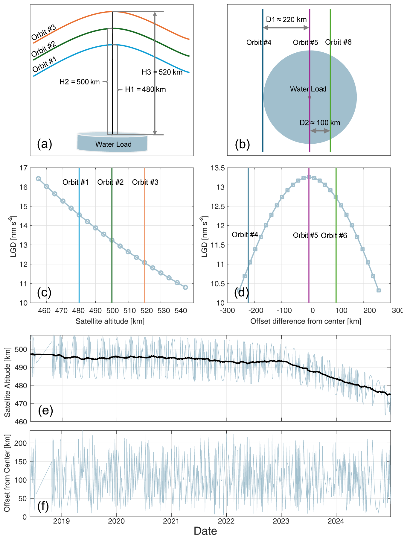
Figure 14 Influence of satellite altitude and track offset on LGD measurements. A uniform water load disk with a thickness of 1 m and a radius of 220 km (∼2° at the equator) is assumed on the Earth's surface (blue disk in panels a and b). Panels (a) and (c) illustrate the altitude effect: three satellite trajectories at 480, 500, and 520 km are simulated above the disk, and the resulting LGD responses show an almost linear increase in signal magnitude with decreasing altitude. Panels (b) and (d) highlight the offset effect: as satellite ground tracks shift laterally away from the disk center, the LGD response decreases, demonstrating strong sensitivity to cross-track displacement. Panels (e) and (f) show the actual GRACE-FO altitudes and ground-track offsets over a 4°×4° block centered on South Sudan during 2019–2024. The black line in panel (e) represents the fitted altitude change.

We further illustrate the real satellite altitude and track offset characteristics over South Sudan (Fig. 14e and f). Since 2022, satellite altitude has decreased significantly (black line in Fig. 14e), implying systematically larger LGD values expected from a given surface mass change. For short-term event detection, such altitude changes would be negligible. However, both altitude variations and track offsets should be addressed in long-term studies, since the orbital changes may bias the regional LGD time series. We therefore recommend that users implement correction strategies to mitigate altitude and offset effects when applying LGD for long-term analyses. Specifically, LGD measurements could be reduced to a common reference observation geometry before regional investigation. Several studies have also attempted to address this issue, for example, by assimilating LGD into hydrological models (Khaki et al., 2023) or by developing inversion approaches (Li et al., 2025a) that account for far-field loading sources (Li et al., 2024). Nevertheless, these should not be regarded as inherent limitations of the LGD dataset itself, but rather as considerations that emerge when LGD measurements are binned and averaged for regional and long-term analyses.

6 Code and data availability

The LGD dataset developed in this study is publicly available at https://doi.org/10.5281/zenodo.17766177 (Tang et al., 2025a). Currently, GRACE-FO LGD dataset is openly accessible, and those will be continuously updated. Results for the GRACE mission will be released in the near future.

The GRACE-FO L1B data used in this study are available at https://podaac.jpl.nasa.gov/GRACE (last access: 29 March 2025) (Wen et al., 2019). The L2 SH products used in this study are the CSR RL06 (GRACE; https://doi.org/10.5067/GRGSM-20C06; UTCSR, 2018) and CSR RL06.3 (GRACE-FO; https://doi.org/10.5067/GFL20-MC063; GRACE-FO, 2024) releases. The kinematic orbit solutions are provided by ITSG at https://ftp.tugraz.at/pub/ITSG/satelliteOrbitProducts/operational (last access: 10 April 2025) (Suesser-Rechberger et al., 2022). The AOD1B products are obtained at https://podaac.jpl.nasa.gov/dataset/grace_aod1b_grav_gfz_rl06 (last access: 10 April 2025) (Dobslaw et al., 2017).

The orbit determination software used in this study is openly available at https://github.com/Thomas-Loudis/georb (last access: 11 July 2025) (Papanikolaou, 2023). The scripts used for forward modeling of the functional LGD are available at https://github.com/mTangcute/spherical-harmonic-synthesis (last access: 31 August 2026; https://doi.org/10.5281/zenodo.21898480, Tang, 2026), and the MCI calculator is available at https://github.com/mTangcute/Mass-Change-Index (last access: 31 August 2026; https://doi.org/10.5281/zenodo.21898480, Tang, 2026).

7 Conclusion

We presented a new dataset of LGD, derived directly from GRACE-FO intersatellite ranging observations with the aid of reference dynamic orbits. The LGD represents the instantaneous gravity differences along the line-of-sight induced by mass variations beneath the satellites. We introduced the different cutoff frequencies for KBR-LGD (10 mHz) and LRI-LGD (20 mHz) used to suppress the instrument noises. In addition to the L1B-derived LGD, we synthesized two functional LGDs: (1) L2-LGD, computed from the L2 monthly mean gravity field solution, and (2) CLM-LGD, computed from a climatological gravity change model. The former highlights the short-term signals in the L1B LGD data in contrast to the monthly mean gravity. The latter enables the derivation of LGD “anomalies” from the climatological mean, that are used to detect and quantify hydrological extremes. The uncertainty analyses show that while instrument noise can be effectively suppressed by band-pass filtering, mismodeled or unmodeled background signals, particularly from AOD, static gravity field, and tidal models, remain the dominant source of error. Through a comparison between regional, time-varying LGD and EWH time series, we derived a scaling relationship indicating that each 1 nm s⁻² change in LGD corresponds to 20–30 mm of surface water storage variation with significant regional variations.

The LGD dataset holds great potential for near real-time monitoring of hydrological extremes when combined with Quick-look Level-1B data. It also can serve as datasets to validate and improve hydrological and geophysical models. The LGD dataset bridges along-track gravimetric observation and water science, making the measurements more accessible and interpretable for hydrologists and paving the way for operational use. This dataset is expected to strengthen on-going GRACE-based hydrological monitoring and expand applications across Earth system science.