CAMS-REG-UNC-v8.1: a detailed uncertainty product for the gridded CAMS-REG-v8.1 emission inventory

Independent verification of greenhouse gas emission reductions and trends in air pollution levels is receiving increasing attention. Atmospheric observations can provide such a constraint on emission estimates through inverse modelling, which requires a detailed quantification of uncertainties in prior emission inventories, observations and chemical transport models. This paper describes a detailed methodology to quantify uncertainties in a state-of-the-art European emission inventory: CAMS-REG. Uncertainties are estimated for all input data used to create the emission inventory and propagated to the final product. This results in separate uncertainty estimates for country-level emissions per sector and uncertainties in the spatial allocation of those emissions. Ideally, the gridded emission uncertainties should add up to the country-level emission uncertainties and for this purpose an optimization procedure was developed (only for countries with detailed emission reporting). This results in (scaled) gridded emission uncertainties and spatial error correlation lengths, which are included in the final dataset. The gridded uncertainty maps show large differences between pollutants and countries, representing the variability in input data and their reliability. CO₂ shows the smallest gridded (optimized) uncertainties, with a median relative standard deviation of 15 % (interquartile range: 9 %–25 %). The largest gridded (optimized) uncertainties are found for NMVOC: 45 % (38 %–58 %). This work follows up from previous efforts and details the first comprehensive emission uncertainty dataset for Europe. The data are available from Zenodo: https://doi.org/10.5281/zenodo.18400810 (Super et al., 2026).

1 Introduction

Effective climate change mitigation and reducing the negative health impacts of air pollution asks for continuous accounting of greenhouse gas and air pollutant emissions. In Europe, most countries report total emissions of both greenhouse gases and air pollutants annually (EMEP, 2023; UNFCCC, 2024). These emissions are based on statistical data of activity rates and estimated emission factors, a so-called “bottom-up” emission inventory. An emission inventory is an accounting system that details how much of a certain trace gas is being emitted to the atmosphere over a specific domain and time window. Emission inventories are widely used to support science and decision-making in the field of air pollution exposure and climate mitigation (e.g., Albarus et al., 2023; Scarpelli et al., 2024; Siouti et al., 2025; Tokaya et al., 2024).

The demand for independent verification of these emission inventories using atmospheric observations is increasing, e.g., in support of the Paris Agreement (European Commission, 2018), to improve national inventories, and to inform national reduction targets (German et al., 2021). Also in the field of air pollution, modelled atmospheric concentrations of air pollutants can be compared to observations for validation purposes and to inform scientists about the accuracy of the emission inventories and atmospheric transport models (e.g., Musollari et al., 2025; Tokaya et al., 2024; Van der A et al., 2024; Wang et al., 2024). When atmospheric observations are used to constrain the input emission data, we refer to this as inverse modelling.

Inverse modelling is a statistical method to optimize a system based on its uncertainties. In the current context, the system consists of input parameters to be optimized (prior emissions), chemical transport models, and atmospheric observations. Here, prior emissions are spatially explicit, which are available at global (Crippa et al., 2018; Doumbia et al., 2021; McDuffie et al., 2020) and regional scales (Gurney et al., 2020; Keita et al., 2021; Kuenen et al., 2022; Kurokawa and Ohara, 2020). In this remainder of this work, we reserve the term “emission inventory” for spatially resolved emission datasets.

The aim of inverse modelling is to find the optimal solution that minimizes the uncertainties at the lowest cost (i.e., the best match between observed and modelled trace gas concentrations). The larger the uncertainty in one of the components, the less information can be gained from it, and the larger the freedom to move away from its starting point. Therefore, a good quantification of uncertainties in each of these components is essential to get reliable output. However, uncertainty quantification in emission inventories is a difficult topic. Often, scientists rely on sensitivity analyses (Lorente et al., 2019), intercomparison studies (Gately and Hutyra, 2017; Hutchins et al., 2017; Oda et al., 2019; Pillai et al., 2016), or expert judgement (Lauvaux et al., 2016; Tenkanen et al., 2024) to estimate the prior emission uncertainty. Error correlations are often neglected, although sometimes a spatial error correlation length is estimated based on expert judgement. A more elaborate study was done by Hogue et al. (2016) for the US, considering multiple sources of uncertainty. However, as far as we are aware, no gridded emission uncertainty data products are currently available, except the work preceding this paper.

This paper describes the methodology developed to quantify uncertainties in the widely-used CAMS-REG European emission inventory. The CAMS-REG emission inventory (Kuenen et al., 2022) is developed by the same researchers that contributed to this paper, which allows us to estimate the uncertainty in each of the input parameters and propagate those uncertainties to the final product. The emission uncertainties are fully consistent for all air pollutants and greenhouse gases in the inventory. Here, we illustrate the full dataset (CAMS-REG-UNC), which builds on previous work (Super et al., 2020, 2024) and now covers uncertainty estimates for all species included in the inventory. A major improvement compared to previous publications is the development of an optimization procedure that ensures consistency between country-level, reported emission uncertainties and the gridded uncertainties through the use of a spatial error correlation length. This allows users to use the dataset at multiple scales and aggregation levels.

2 Methods

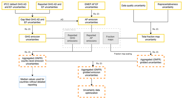
Estimating uncertainties in data products can be done in different ways. Here, we choose to define uncertainties at the most detailed level possible and propagate those uncertainties to the final product (Fig. 1). This work is done by the same group of researchers responsible for processing the emissions data, which allows us to take stock of the detailed knowledge of the input parameters and assumptions that are made during the preparation of the CAMS-REG inventory.

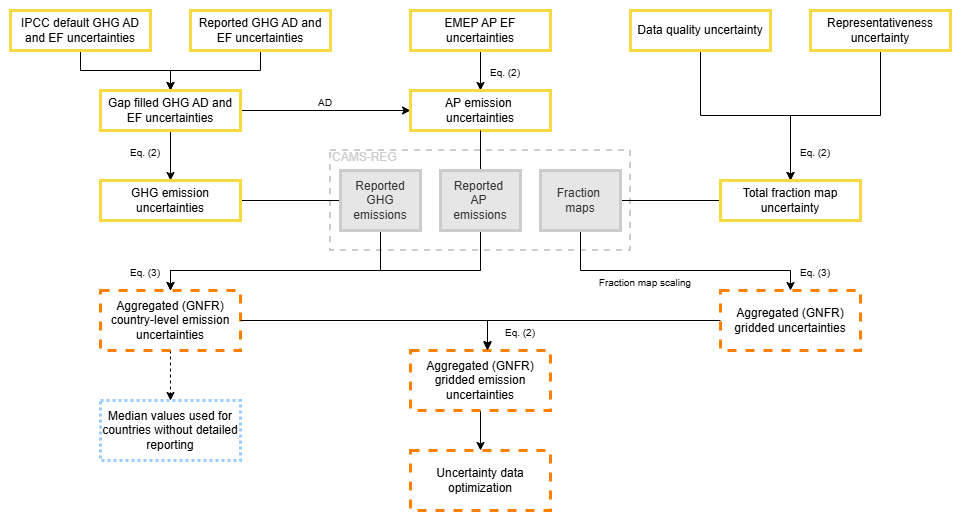
Figure 1 Flow diagram showing the error propagation process for countries with detailed emission reporting, including a reference to the equations used and explained in Sect. 2.3. Yellow, solid boxes are related to the uncertainty input and orange, dashed boxes to the aggregated (GNFR: Gridded Nomenclature For Reporting) uncertainty output. The blue dotted box indicates where the emission uncertainties for countries without detailed emission reporting come from. GHG and AP refer to greenhouse gases and air pollutants, respectively. AD and EF refer to activity data and emission factors, respectively.

In the following sub-sections, we describe the emission inventory, the sources of uncertainty, the data used to estimate those uncertainties, and the processing steps to get to the final product. The processing steps are different for countries with detailed emission reporting (Annex-I countries), other countries (mostly North Africa and Middle East), and sea regions (see Table A1 for a list of regions and to which category they belong). Note that some of these methods have been described previously (Super et al., 2024), but several changes and improvements have been made.

2.1 European emission inventory

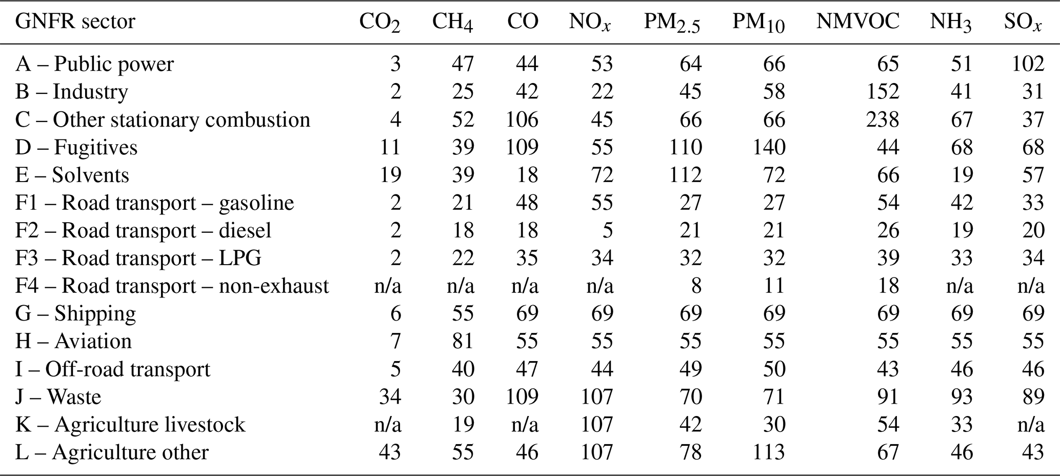
The emission inventory used as a basis for this work is the CAMS-REG v8.1 for 2022, described in detail by Kuenen et al. (2022). This emission dataset is the state-of-the-art gridded emission inventory for Europe with a spatial resolution of 0.1° by 0.05°. It contains emissions of greenhouse gases (CO₂, CH₄) and air pollutants (CO, NO_x, PM_2.5, PM₁₀, NMVOC, NH₃, SO_x) per GNFR (Gridded Nomenclature For Reporting) sector, with an additional split for road transport, as indicated in Table 1.

Table 1 Overview of GNFR sectors and the 95 % confidence interval (in %) of emissions for countries without detailed emission reporting. These intervals are based on the median GNFR-level uncertainties for countries with detailed emission reporting (see Sect. 2.2.1). n/a = not applicable.

The CAMS-REG emission inventory is based as much as possible on emission reports from individual countries. For greenhouse gases, Annex-I countries report their emissions on an annual basis to the UNFCCC (UNFCCC, 2024) and for air pollutants emission reports are delivered to the EMEP (European Monitoring and Evaluation Programme) Centre on Emission Inventories and Projections (EMEP, 2023). These reports contain country-level emissions for over 250 detailed sector/fuel combinations, which are spatially distributed using a wide range of fraction maps. Fraction maps describe the share of the country-level emissions occurring within each grid cell based on spatial proxy data (e.g., population density or land use), and therefore their sum is always one for a country. Finally, the gridded emissions are aggregated to the GNFR sectors.

Most shipping activities are of international nature, taking care of transport between countries, and are therefore not included in national total emissions. Some countries report (part of) the international shipping emissions, but these provide an incomplete picture of shipping emissions in Europe. Therefore, CAMS-REG uses the shipping emissions from the STEAM model (Jalkanen et al., 2012; Johansson et al., 2017), that provides gridded emissions on the CAMS-REG grid definition. The emissions are based on AIS (Automatic Identification System) data and vessel characteristics and cover all pollutants in the CAMS-REG dataset. Additionally, for countries without detailed emission reporting, where emission reporting is incomplete, or the quality of the reporting is poor, other datasets are used to estimate emissions per GNFR sector.

2.2 Emission uncertainty estimates

The main source of uncertainty in the emission inventory is related to the input data used for the CAMS-REG inventory (see also Fig. 1). The reported annual, country-level emissions have an uncertainty, which is determined largely by the applied methodology and the quality of the data used for those calculations. For example, countries can decide to use a default method or emission factor, or a country-specific approach. Generally, the first option results in a higher uncertainty. Additionally, we identify two sources of uncertainty in the spatial disaggregation. First, the quality of the proxy data itself is a source of uncertainty. For numerical data, the data quality indicates the accuracy of the values provided. For categorial variables, this often translates into a correct categorization of each grid cell, for example whether a grid cell identified as grassland is indeed grassland. Second, an important source of uncertainty is the representativeness of a proxy, i.e., how well does a proxy represent the actual location and magnitude of activities that cause emissions.

The data used to estimate these uncertainties are detailed in the next sub-section. Other sources of uncertainty are, for example, the discrete nature of the grid and possible double-counting or missing sources (systematic errors). We do not consider these sources of uncertainty in this study.

2.2.1 Country-level emission uncertainties

Most Annex-I countries that report their greenhouse gas emissions also include an uncertainty estimate, although this is not mandatory. This uncertainty estimate can be more or less detailed in terms of sector (dis)aggregation, but at least provides an uncertainty for activity data (AD) and emission factors (EF) separately and often differentiates between fuel types.

First, we collected the reported uncertainties from 29 countries for the reporting year 2020 (UNFCCC, 2024). Generally, the reported uncertainties vary little from one reporting year to the next, except for some typos or when the methodology for the emission calculations has changed. A few typos identified for Italy were corrected based on a discussion with the reporting agency. Although more typos may occur, we are unable to identify those without detailed knowledge of the methodologies applied by each country and a discussion with the reporting agencies, which would be impossible to achieve. Therefore, we assume the reported uncertainties to be valid for the year considered. Estonia provided multiple uncertainty estimates for several sectors, separating between different activities within a sector, and we made an assumption about the most dominant activity. This did not occur for other countries.

Second, gap filling is applied to cover all sector/fuel combinations and countries. If a country reports uncertainties at a more aggregated sector level, we assume this uncertainty to be representative for the more detailed sub-sectors, but only up to a certain level. For example, uncertainties for road transport can be used for all vehicle types, but a more aggregated uncertainty (e.g., for mobile sources as a whole) is assumed to be unreliable. Next, for each sector/fuel combination, we take the uncertainties from all countries that report an uncertainty, and calculate the median value. This median value is then applied to all countries without uncertainty information for that particular sector/fuel combination after applying the first gap filling step. In very few cases uncertainty information is lacking completely for a specific sector/fuel combination and IPCC default values are used (Eggleston et al., 2006).

Air pollutant emission uncertainties are generally not reported by the countries. However, in most cases, the AD is shared between the greenhouse gases and air pollutants and the reported greenhouse gas AD uncertainty is used consistently for all trace gases. The EMEP/EEA Guidebook provides a global Tier-1 uncertainty estimate for the air pollutant EFs (European Environment Agency, 2019), which is applied to all countries. Additionally, a generic uncertainty range is applied to sector/fuel combinations without an uncertainty estimate, as listed in Chapter 5 of the EMEP/EEA Guidebook. The range is chosen based on expert judgement of the quality of the EF estimate.

The greenhouse gas and air pollutant emission uncertainties are propagated to the GNFR level (explained in Sect. 2.3). The median GNFR-level emission uncertainties are applied to countries without detailed emission reports (Table 1, Fig. 1).

International shipping falls under the same GNFR category as inland shipping, but it is treated separately, as the emissions are not reported by countries. The AD uncertainty estimate for international shipping is based on a comparison of the STEAM model predictions with fuel reporting (Jukka-Pekka Jalkanen, personal communication, 25 August 2022). Emission factors uncertainties are estimated by Grigoriadis et al. (2021).

A table with country-level emission uncertainty ranges per sector/fuel combination is provided as Supplement.

2.2.2 Proxy data uncertainties

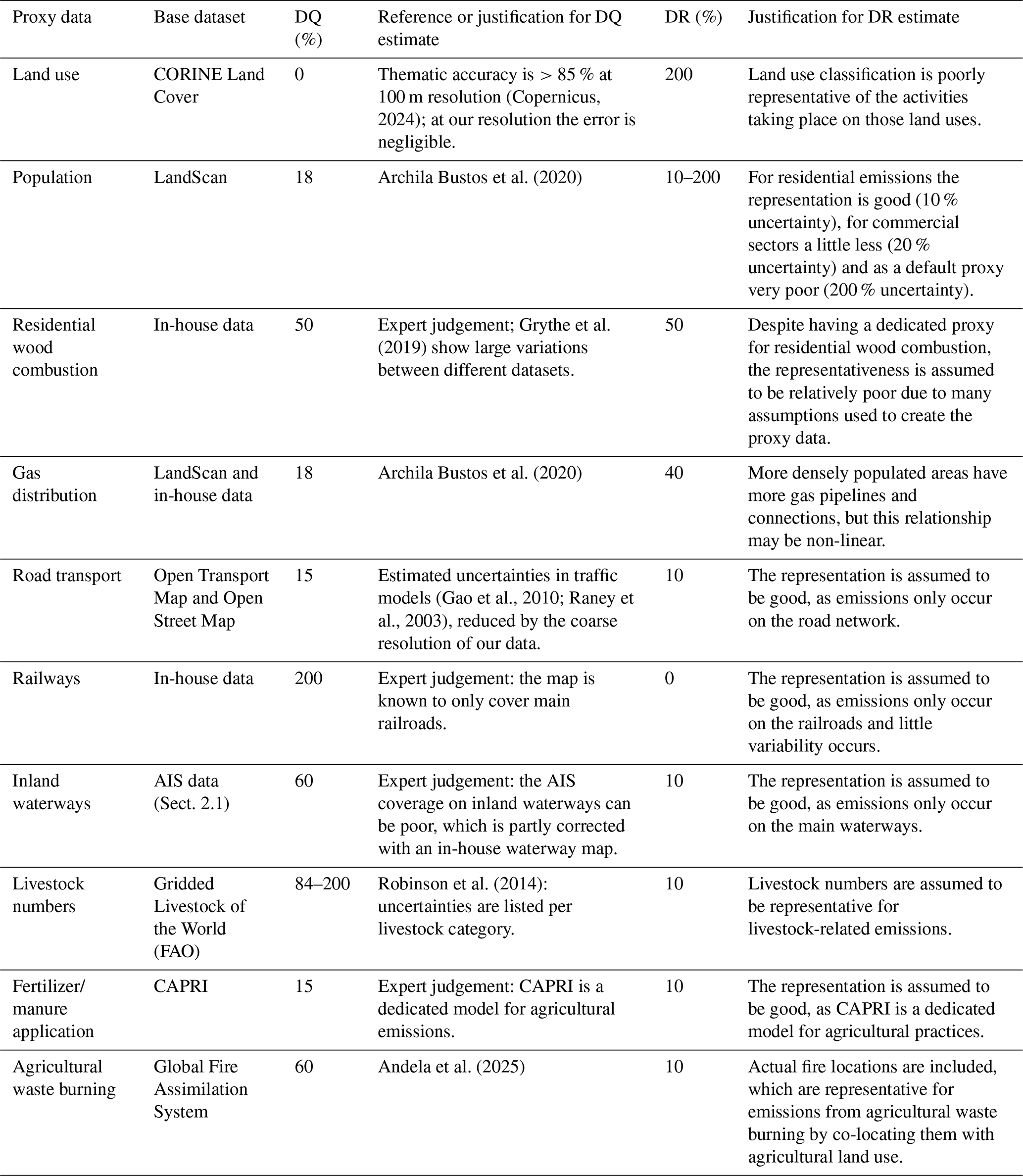
The proxies used for the spatial disaggregation of country-level emissions are mostly based on open-source datasets, sometimes processed to better represent the spatial patterns in emission activities. Therefore, the data quality uncertainty is taken from metadata or publications from the providers of those datasets, where possible. In some cases, the uncertainty estimates of other, similar datasets are used. Where such information is not available expert judgement was needed. The uncertainty values are summarized in Table 2, including the source of these estimates and the base datasets used to create the proxies. For more details about the spatial proxies we refer to Kuenen et al. (2022).

Table 2 Overview of proxy data (in general terms) and the uncertainties (95 % confidence interval) related to the quality of the data (DQ) and the data representativeness (DR). For the data quality, references to uncertainty estimates in the base dataset or similar datasets are listed where possible, and for the representativeness error a justification is provided.

It is important to note that if grid cells falsely contain no data (zero value or the wrong category) this cannot be solved in an inversion system by including an uncertainty estimate (scaling a value of zero remains zero). This also affects point source locations. We have seen examples where the coordinates of an industrial facility were actually pointing to the headquarters of the company, which could be at a completely different location than where the emitting activity takes place. Therefore, a lot of resources have been invested in placing large point sources at their correct location and we assume the spatial allocation of point sources has no uncertainty.

The locations of most sources are relatively well-known, but the actual activity rate at any given location may be more difficult to assess through spatial datasets. For example, the road network is well-known, but traffic intensity may vary strongly between road segments. Similarly, population may be a reasonable proxy for residential combustion emissions, but in more densely populated areas the fuel consumption per household is often lower than in rural areas. Therefore, we add a representativeness error for each proxy, which is based on expert judgement (see Table 2 for a justification). Whereas the data quality is always the same for a proxy, the representativeness error depends on the sector it is applied to. For example, population is sometimes used as a default proxy and in that case the error is larger than when it is used for residential combustion.

The representativeness error increases the uncertainty per grid cell, but it also causes errors to be spatially correlated between grid cells that are nearby and have similar characteristics. This is expressed through a spatial correlation length, which will be explained in more detail in Sect. 2.4.

For countries without emission reporting we take spatially explicit emissions directly from other datasets and the proxy maps are not applied. As we lack information on the reliability of the spatial patterns in those datasets, we set the spatial uncertainty to 200 % (95 % confidence interval) for all GNFR sectors. For international shipping we set the spatial uncertainty to 60 % (95 % confidence interval), based on the accuracy and coverage of the AIS data and additional uncertainties in the STEAM model.

2.3 Error propagation

In the previous sections we presented the uncertainty input. The next step is to combine the uncertainties at this high level of detail to more aggregated values that match the level of detail in the emission inventory. In other words:

1. We need to combine uncertainties in AD and EF per sector/fuel combination to get uncertainties in emissions, and aggregate this per GNFR sector and country.

2. We need to combine the data quality and representativeness error for each proxy to get uncertainties in the spatial allocation, and aggregate this per GNFR sector and grid cell.

3. We need to combine the uncertainties in country-level emissions and the spatial allocation from the first two steps to get total gridded emission uncertainties per GNFR sector.

These steps are also visualized in Fig. 1. For all steps, we apply a simple error propagation method assuming no error correlations exist. However, regular error propagation makes use of standard deviations, whereas the uncertainties presented here are provided as a normalized 95 % confidence interval. Moreover, error propagation assumes all error distributions are Gaussian, whereas many of our parameters have a lognormal error distribution. Therefore, we need to derive a Gaussian relative standard deviation from the confidence interval:

$$\begin{array}{}\text{(1)}& {\displaystyle \frac{{\mathit{\sigma }}_X}{X}}={\displaystyle \frac{(\ln \left({\lim }_{\mathrm{upper}}\right)-\ln \left({\lim }_{\mathrm{lower}}\right))}{\mathrm{4}}}.\end{array}$$

Here, lim_upper and lim_lower are the upper and lower limit of the 95 % confidence interval of variable X, respectively. Moreover, σ is the standard deviation of variable X and the standard deviation divided by the parameter value denotes a relative uncertainty.

For the first step, we combine the AD and EF uncertainties. For countries with detailed emission and uncertainty data, the emissions are a product of the AD and EF. Therefore, the relative standard deviations of AD (variable X) and EF (variable Y) can be used in Eq. (1) to estimate the relative uncertainties in emissions (variable Z):

$$\begin{array}{}\text{(2)}& {\displaystyle \frac{{\mathit{\sigma }}_Z}{Z}}=\sqrt{{\left({\displaystyle \frac{{\mathit{\sigma }}_X}{X}}\right)}^{\mathrm{2}}+{\left({\displaystyle \frac{{\mathit{\sigma }}_Y}{Y}}\right)}^{\mathrm{2}}}.\end{array}$$

The emission uncertainties per sector/fuel combination i are then aggregated to the GNFR sector (agg):

$$\begin{array}{}\text{(3)}& {\mathit{\sigma }}_{z,\mathrm{agg}}=\sqrt{\sum _i^n{{\mathit{\sigma }}_{z,i}}^{\mathrm{2}}}.\end{array}$$

In Eq. (3) we use absolute standard deviations, so we need to multiply the output from Eq. (2) with the emission values.

For the second step, the data quality (variable X) and representativeness (variable Y) errors are combined following Eqs. (1) and (2) to get the total relative uncertainty for a spatial proxy (variable Z). Next, these spatial uncertainties are aggregated to the GNFR sector following Eq. (3). However, we cannot directly use the gridded fractions as variable Z to calculate the absolute standard deviations, as the sum of all fractions per country and sector needs to be equal to one for an aggregated sector. Therefore, we scale each fraction map based on its relative contribution to the GNFR sector emissions per trace gas and country. These scaled fractions are then used as variable Z to calculate the absolute standard deviations used in Eq. (3). Note that, even though the uncertainty per proxy is the same all over the domain, the final gridded uncertainties per GNFR sector vary per grid cell due to the different contributions of each proxy in a grid cell.

For the final step, we add the uncertainties in country-level emissions from step 1 to the uncertainties in the grid cells belonging to that country from step 2 using Eq. (2) per GNFR sector and trace gas. With this, we cover uncertainties in the emissions and the spatial distribution.

For sea shipping, first Eq. (2) is applied to calculate the emission uncertainty per sea region, and then this value is combined with the spatial uncertainty. For countries without detailed emission reporting, only this final step is applied, as all input parameters are already specified at the GNFR emission level. In both cases, the gridded uncertainty shows no spatial variability.

2.4 Uncertainty data optimization

The previous steps provide gridded emission uncertainties based on uncertainties in the input data. The sum of all gridded emission uncertainties within one country should match the country-level uncertainty calculated in step 1 in the previous section. However, this is not the case, as the uncertainties in the proxies are independent from the country-level data. Therefore, we developed an optimization procedure, which matches the sum of the gridded uncertainties to the country-level uncertainties by introducing a spatial error correlation length. The reason for setting the country-level uncertainties as our benchmark is that these are well-documented and consistent across the domain.

We can think of the gridded emission uncertainties within a country as diagonal elements in a covariance matrix (σ(X_i)²), where X_i represents one element from n gridded uncertainties). The sum of all elements is the total country-level uncertainty, assuming no error correlations exist:

$$\begin{array}{}\text{(4)}& {\mathit{\sigma }}_{\mathrm{sum}}=\sqrt{\sum _i^n\mathit{\sigma }{\left(X_i\right)}^{\mathrm{2}}}.\end{array}$$

The sum of these elements (σ_sum) should be equal to the reported country-level uncertainties (σ_country). When this criterion is not met, we can introduce error correlations. Whereas uncorrelated errors tend to cancel each other out, positively correlated errors add up to larger total uncertainties. Therefore, we introduce a covariance in Eq. (4):

$$\begin{array}{}\text{(5)}& {\mathit{\sigma }}_{\mathrm{sum}}=\sqrt{\sum _i^n\mathit{\sigma }{\left(X_i\right)}^{\mathrm{2}}}+\sum _i\sum _{j\ne i}\mathrm{Cov}\left(X_i,X_j\right).\end{array}$$

Here, Cov(X_i,X_j) is the covariance between elements X_i and X_j from n gridded uncertainties, which is a function of the uncertainties in X_i and X_j and their error correlation.

Next, we need to quantify the error correlations. Gridded emissions errors are more likely to be correlated when they are spatially close together. Gridded emissions that are far apart are unlikely to exhibit the same errors. Therefore, we introduce a spatial error correlation length L, which is used to define the error between two grid cells, following an exponential decay with distance:

$$\begin{array}{}\text{(6)}& r_{i,j}=e^{-d_{i,j}/L}\mathrm{for}L\ge \mathrm{0}.\end{array}$$

Here, r is the (positive) correlation coefficient between location i and j, d is the distance between location i and j, and L is the spatial correlation length, following Kunik et al. (2019). The smaller the distance between two grid cells, the stronger the correlation in their emission errors. These error correlations are now used in Eq. (5). As mentioned before, it is fair to assume spatial error correlations exist related to the representativeness error in the fraction maps.

There are two options to solve Eq. (5). Option one is to choose a spatial error correlation length such that the sum of the variances and covariances equals the country-total uncertainty, but this can result in unrealistic values for the correlation length. Option two is to pick a reasonable correlation length and scale the gridded uncertainties. However, we wish to maintain the physical properties of the emission inventory, such that the uncertainties are physically meaningful as well. Therefore, we choose a flexible approach, as depicted in Fig. 2, which first tries to select an appropriate correlation length within certain bounds and, if this does not result in a good agreement, it scales the gridded uncertainties. Note that the optimization is done per country and we assume no error correlations exist between pollutants and sectors.

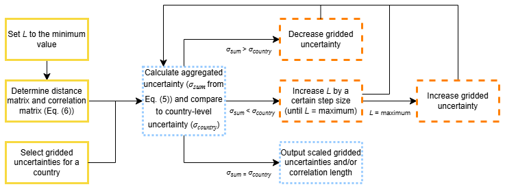
Figure 2 Flow diagram showing the optimization procedure for the gridded uncertainties. Yellow, solid boxes are related to the initialization and orange, dashed boxes to the optimization.

The first step in the process is to determine a distance matrix, which is done using the Spherical Law of Cosines (Kuipers, 1999; Van Brummelen, 2017). Based on this, we can formulate a correlation matrix, using Eq. (6). The minimum correlation length is set to 0 km and the maximum correlation length to half the maximum distance between two grid cells within the country. Next, we calculate the aggregated uncertainty (Eq. 5) for both the minimum (σ_sum,min) and maximum (σ_sum,max) correlation length and compare the results against the reported country-level uncertainty. If σ_sum,min exceeds σ_country the gridded uncertainties are scaled down and L remains zero. If σ_country exceeds σ_sum,max the correlation length is set to its maximum value and the gridded uncertainties are scaled up. In all other cases, Brent's method (Press et al., 1992) (using Python's Scipy package) is used to find the optimal correlation length and no scaling is applied to the gridded uncertainties. The output of the optimization is a scaling factor for the gridded uncertainties and a spatial error correlation length per country, sector and pollutant.

Countries without detailed emission reporting and sea regions have no reliable region-total uncertainty and therefore the optimization is not applied to those regions. Russia is also excluded from the optimization, as it only falls partially within our domain and therefore the sum of the gridded uncertainties do not necessarily have to match the country-level uncertainties. Moreover, point sources are excluded from the optimization. As we assume no spatial uncertainty for point sources, no spatial error correlation exists between them and their uncertainty consists only of the emission uncertainty. We subtract point source emissions and their uncertainty contribution from the country-total emissions and uncertainty before running the optimization. This means the spatial error correlation length should only be applied to the area sources.

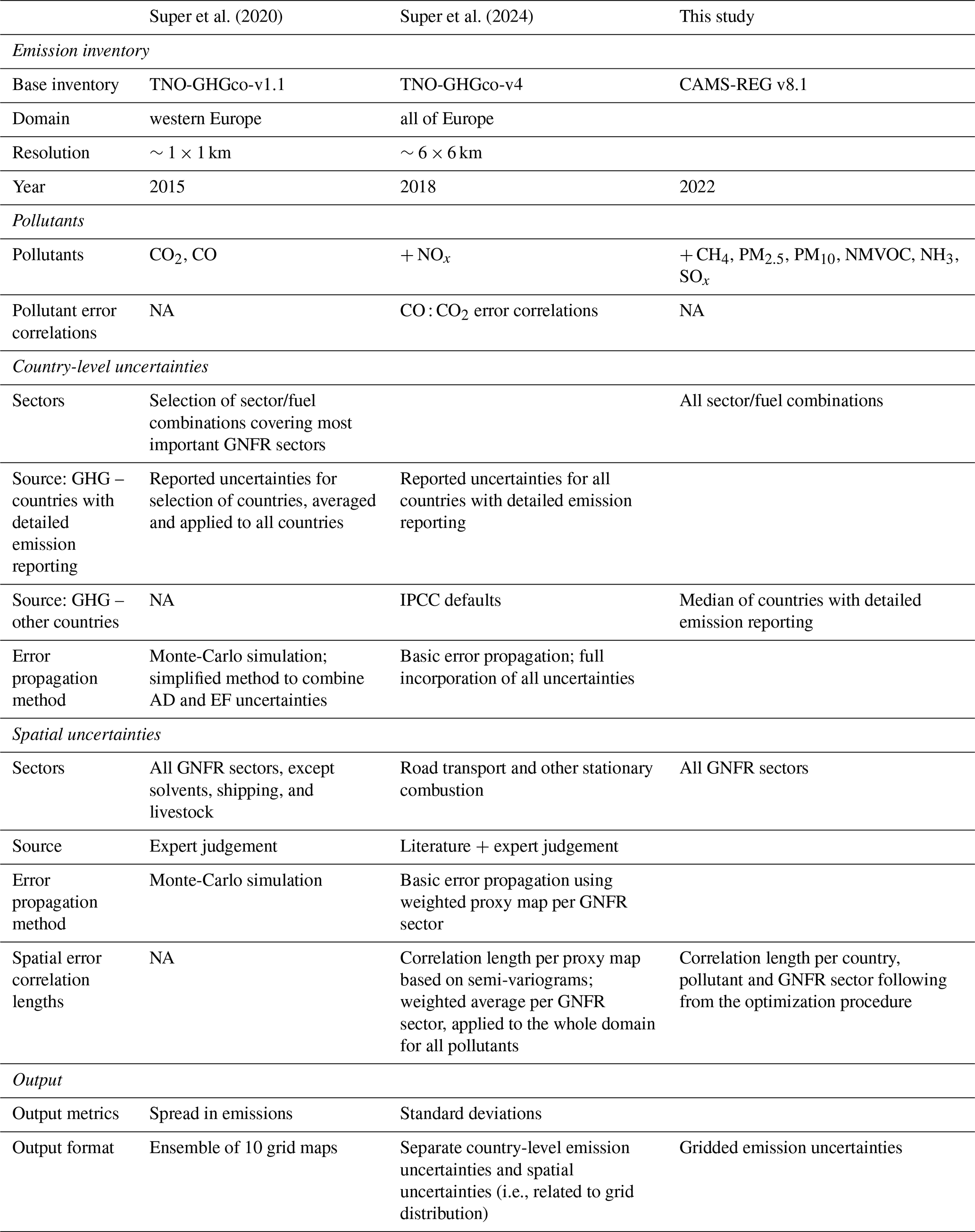
2.5 Differences with previous versions

The work described in this paper builds on previous studies on gridded emission uncertainties (Super et al., 2020, 2024). Each version has received updates based on new insights and improved prior knowledge. Moreover, over the years, more pollutants and sectors are included. Therefore, we expect new versions to outperform older versions, despite the large number of assumptions and high uncertainties in our input. Nevertheless, each version has its own valuable characteristics that could be useful for specific implementations.

To better understand the differences between these products we summarize the main characteristics in Table 3. The version described in Super et al. (2024) has had major updates in methodology compared to the first version. The error propagation method has been changed from a Monte-Carlo simulation to basic error propagation, which is much less expensive and still performs well enough (as illustrated in Super et al., 2024). Moreover, the domain was extended, country-specific emission uncertainties were included, and spatial error correlation lengths were introduced. The methodological updates in the work presented here are mostly limited to the optimization procedure. This gives us a different estimate of the spatial error correlation lengths, which are much larger than in the previous version to align the gridded and country-level emission uncertainties. Moreover, we have extended the dataset to cover all pollutants and sectors included in the emission inventory.

Table 3 Overview of emission uncertainty datasets preceding and including this study. Only changes compared to the previous version are included and a blank space means nothing has changed. If specific characteristics are not included in a particular dataset, while they were included in a previous version, we have put NA in the table.

3 Results

Most results are presented in violin plots. In these plots, the lower and upper horizontal lines represent the interquartile range (IQR; Q₁ to Q₃), and the middle line indicates the median (Q₂). The width of the blob represents the probability density of the data at each value. All uncertainties are presented as relative standard deviation (σ), unless explicitly mentioned otherwise.

3.1 Country-level emission uncertainties

The country-level emission uncertainties form the basis of the final product, as they serve as direct input to the error propagation process and as a constraint in the optimization. Therefore, they have a significant impact on the final uncertainties.

Figure 3 shows the spread in country-level emission uncertainties per pollutant, for which the sectoral uncertainties are aggregated per country. The CO₂ emission uncertainties are low – 0.01 (median) (0.01–0.02 (IQR)) –, because the emission factors are well-known and stable. Moreover, CO₂ emissions are predominantly from combustion activities, for which activity data are easier to estimate than, for example, fugitive emissions. Additionally, the range in country-level emission uncertainties for CO₂ is small, because the reported uncertainties are very similar across countries.

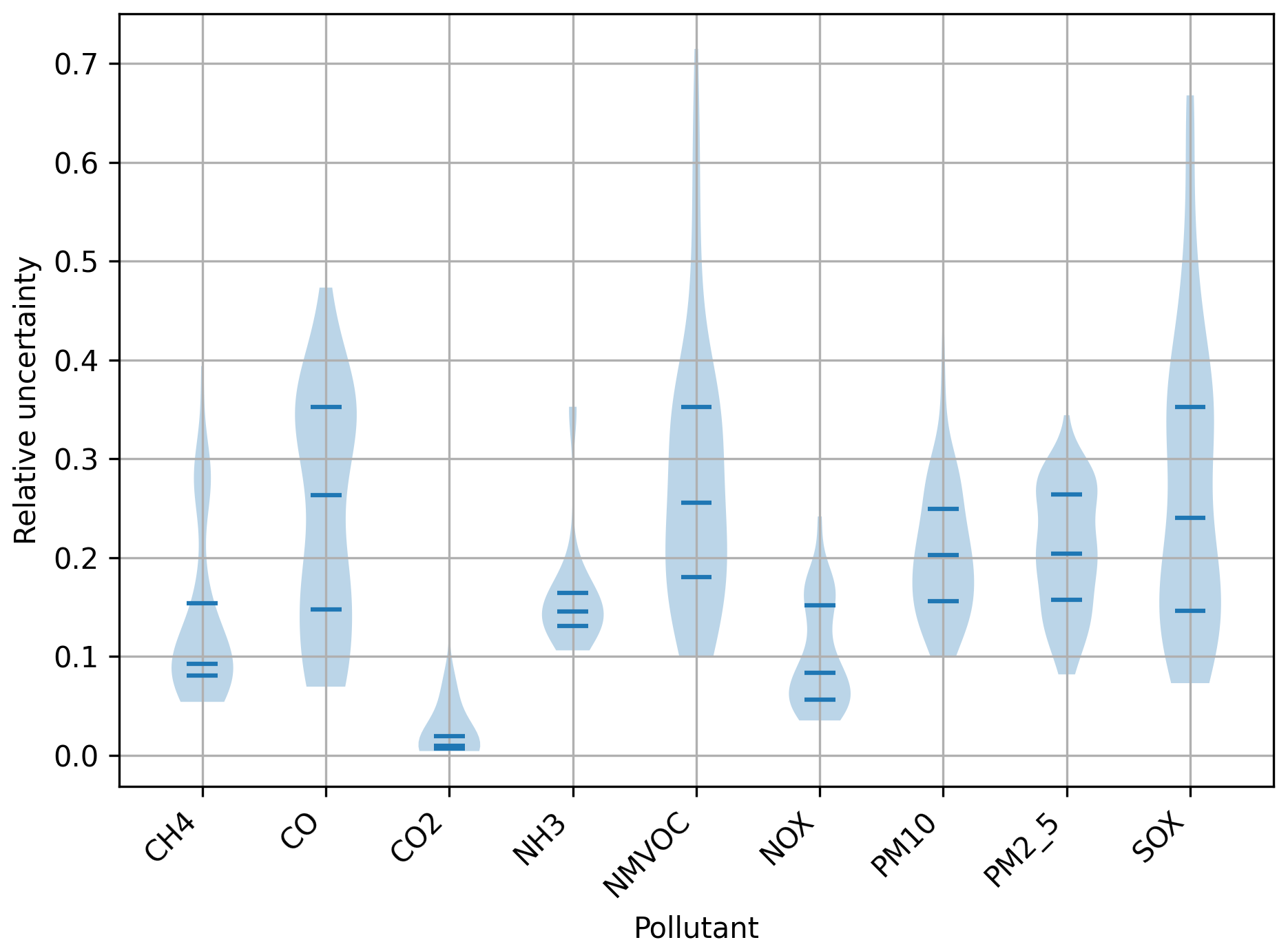
Figure 3 Violin plot of total country-level emission uncertainties (summed over all sectors) per pollutant.

Figure 4 Violin plot of country-level CO emission uncertainties per sector.

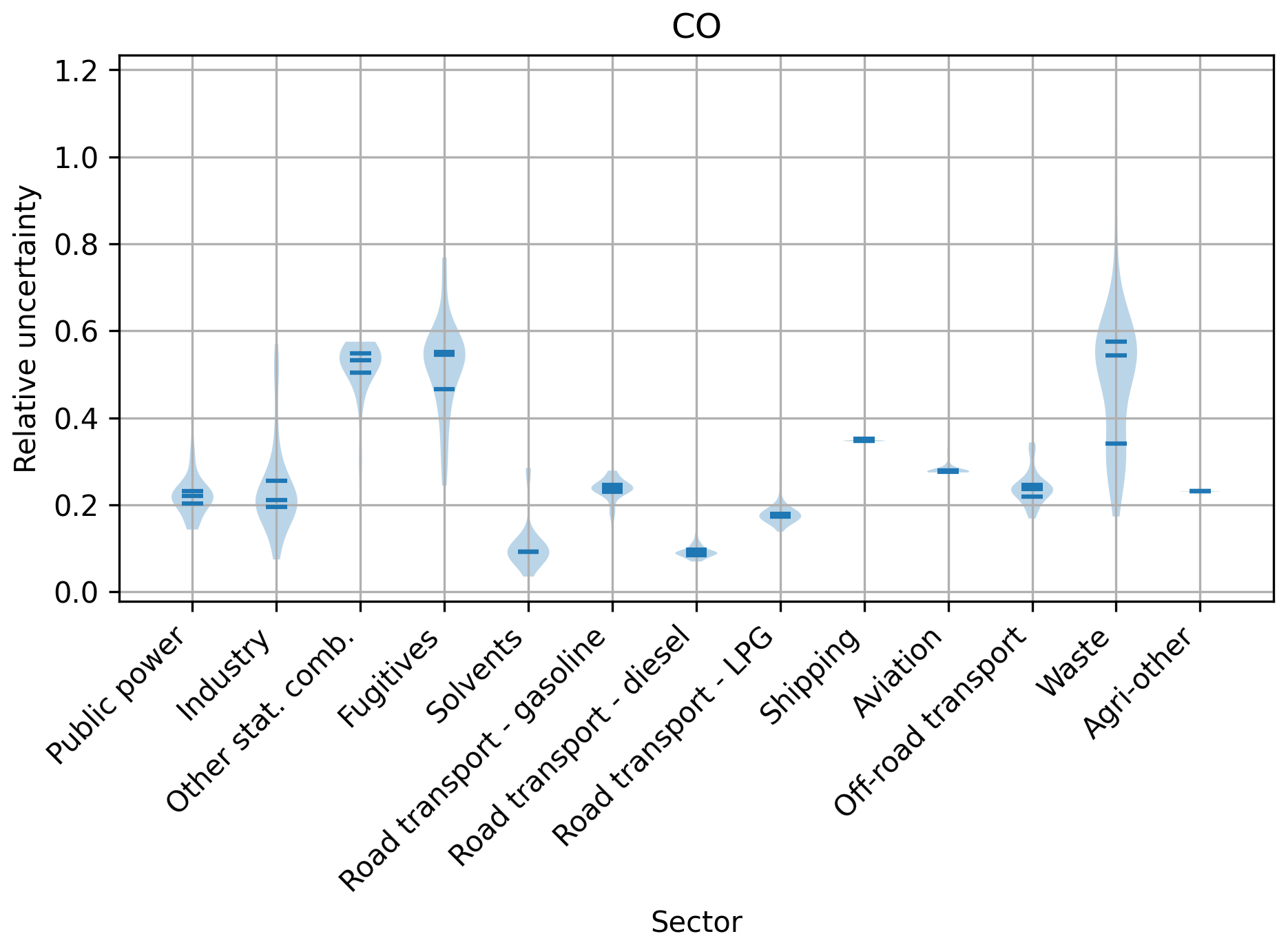
In contrast, the uncertainty ranges for SO_x (0.24 (0.15–0.35)), NMVOC (0.26 (0.18–0.35)) and CO (0.26 (0.15–0.35)) are large, which is related primarily to the significantly larger uncertainty in emission factors of the dominant emission sectors compared to CO₂. Figure 4 shows the spread in country-level CO emission uncertainties per sector. The other stationary combustion sector has a high emission uncertainty and can be a major source of CO emissions in a country. For example, in Estonia about 57 % of all CO emissions come from the other stationary combustion sector, which results in a country-total uncertainty of 39 %. In other countries, the contribution from this sector can be relatively small, for example, when the main fuel type is natural gas or limited heating is needed due to a warm climate. In Iraq, over 90 % of all CO emissions are attributed to road transport, which has a much lower uncertainty, and the country-total uncertainty adds up to 14 %. Hence, the country-level uncertainty depends on the sector contributions and the emission uncertainty associated with the dominant sectors.

The uncertainty ranges for CH₄, NH₃, NO_x, PM₁₀, and PM_2.5 are (0.09 (0.08–0.15)), (0.15 (0.13–0.16)), (0.08 (0.06–0.15)), (0.20 (0.16–0.25)), and (0.20 (0.16–0.26)), respectively.

3.2 Gridded emission uncertainties

The final product consists of gridded uncertainties, which have been optimized for countries with detailed emission reporting (Sect. 2.4). The uncertainties are presented as a relative standard deviation, and can be translated into absolute standard deviations using the gridded emission values. Both relative and absolute gridded emission uncertainties for selected pollutants are shown in Fig. 5 (area sources only).

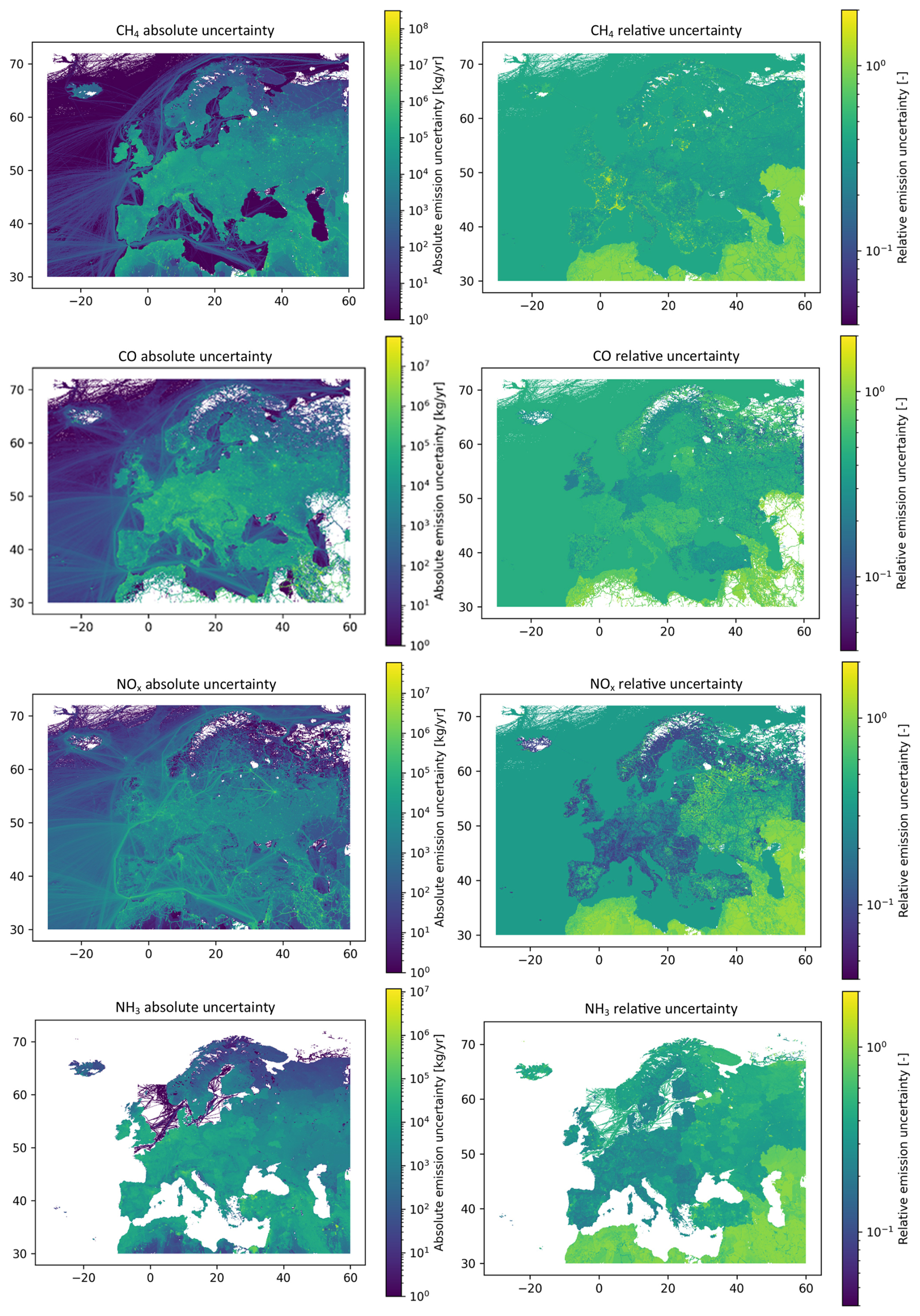
Figure 5 Maps of absolute and relative gridded emission uncertainties for selected pollutants. All colour scales are logarithmic, where the same scale is applied for the relative uncertainties.

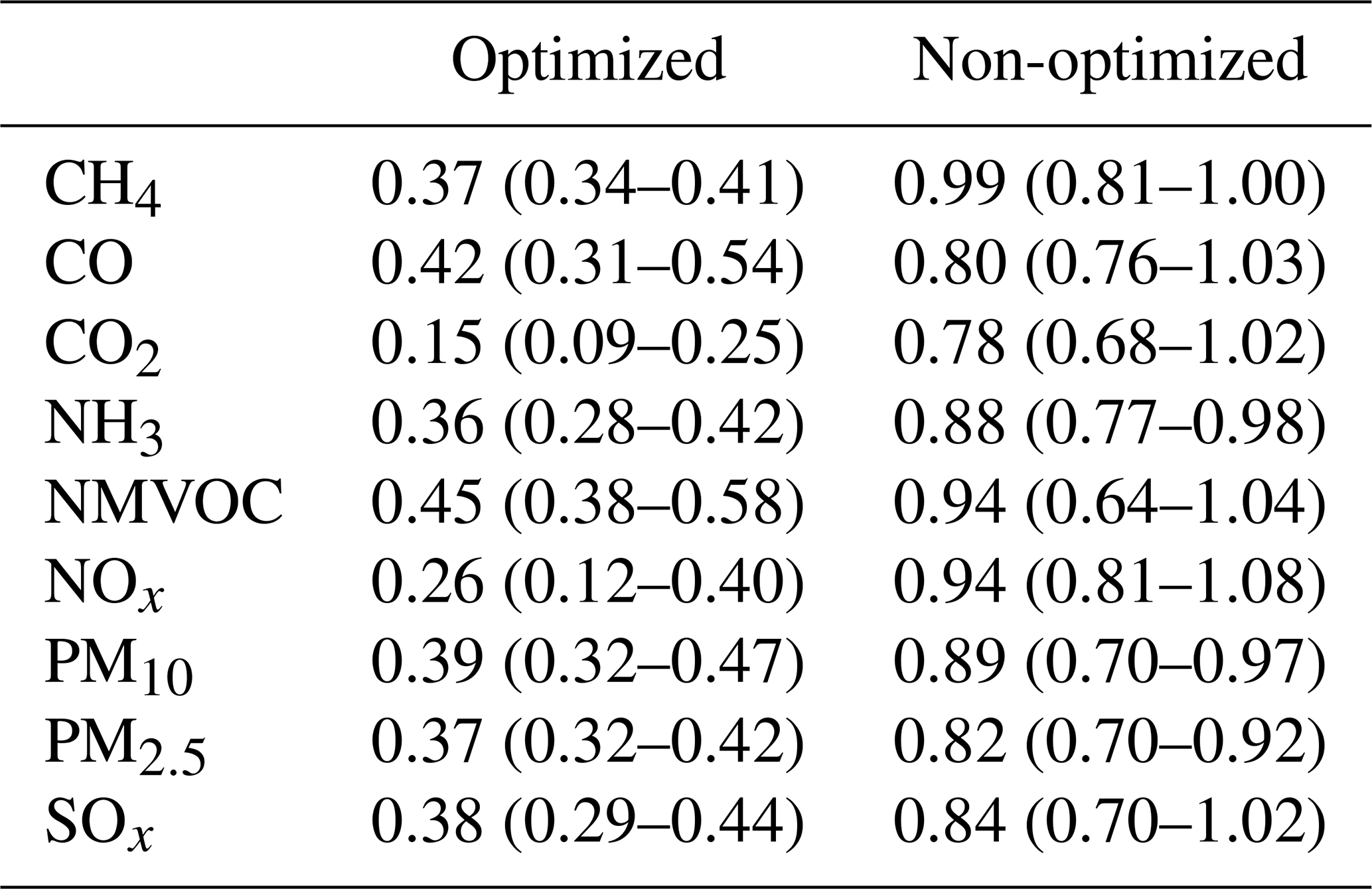
A summary of the gridded uncertainties is provided in Table 4. In this table, results are reported separately for countries with detailed emission reporting and optimization (column “Optimized”) and for countries without detailed emission reporting and optimization (column “Non-optimized”). The gridded uncertainties are higher for the non-optimized countries, because we assign a high uncertainty to the spatial distribution of emissions in those countries (Sect. 2.2.2).

Table 4 Summary of median (IQR) relative uncertainties for countries with detailed emissions reporting and optimization (Optimized) and for countries without detailed emissions reporting and optimization (Non-optimized).

The absolute uncertainties follow largely the spatial patterns in emissions, with high absolute uncertainties in those places where high emissions occur. The maps of relative uncertainties show large jumps between countries, which is due to differences in the total country-level emission uncertainties. A country with a high overall uncertainty will, in general, receive larger gridded uncertainties. However, these patterns differ per pollutant. While CH₄ shows a relatively smooth relative uncertainty over Europe, CO and NH₃ show particularly large differences between countries. The sector mix will have a large impact on these patterns, as discussed before.

3.3 Optimization parameters

The final product contains spatial error correlation lengths, following from the optimization procedure. These correlation lengths are defined for each specific country/sector/pollutant combination and should be applied to the area sources only (point sources have no correlation length). Note that correlation lengths are only available for countries for which the optimization procedure was performed (N=41).

Figure 6 shows the spread in country-specific correlation lengths and scaling factors per pollutant, averaged over all sectors. The average correlation lengths are often larger than zero. This means that spatial correlations play an important role in ensuring that the gridded uncertainties do not cancel each other out at the country-level. Generally, the larger the country, the larger the correlation length needed. The median scaling factors are generally slightly above one, meaning that with the maximum correlation length the country-total uncertainty is not sufficiently high and the gridded uncertainties are upscaled.

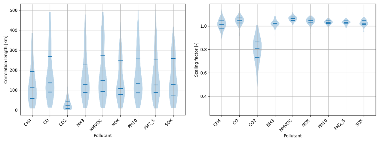
Figure 6 Violin plot of country-specific correlation lengths (left panel) and scaling factors (right panel) per pollutant, averaged for all sectors.

An exception is CO₂, which often shows scaling factors smaller than one. The reason is that the country-level uncertainties for CO₂ are small and summing up all gridded uncertainties leads to a larger combined uncertainty than what the countries report. Therefore, gridded uncertainties are downscaled and correlation lengths are often zero.

The largest correlation lengths appear for road transport, waste and other stationary combustion (Fig. 7). For these sectors, the sum of the gridded uncertainties is too small to end up with the country-level emission uncertainty. This also results in occasional upscaling of the gridded emission uncertainties. In contrast, gridded uncertainties from the public power and industry sectors are often downscaled and receive low correlation lengths.

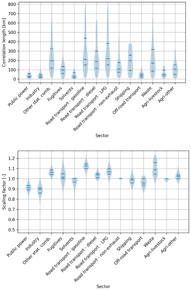
Figure 7 Violin plot of country-specific correlation lengths (top panel) and scaling factors (bottom panel) per sector, averaged for all pollutants.

These results illustrate the importance of the optimization procedure. Without this step, the gridded and country-level emission uncertainties would be inconsistent. The optimized data, in combination with the spatial error correlation lengths, allow users to work with the data at any spatial resolution.

4 Discussion

4.1 Comparison to other uncertainty estimates

The quantification of gridded emission uncertainties is a complex process and relies heavily on the inventory's source data and processing steps. We present an uncertainty estimate that propagates the uncertainties from the source data to the final product, following all the steps taken in the inventory preparation, ensuring consistency between the gridded emissions and their uncertainties. Previous efforts to estimate emission uncertainties have resulted in a wide range of uncertainty values. The number of studies looking quantitatively at gridded emission uncertainties is, however, limited. We discuss the most relevant scientific research below, starting with country-level/regional emission uncertainties, for which more studies are available. We list all uncertainties as relative standard deviation, unless indicated otherwise.

In this work, we use, where possible, reported country-level emission uncertainties at a detailed sector/fuel level. Most countries use a Monte Carlo simulation to calculate these uncertainties, and we consider them relatively reliable. Differences between countries occur mostly when the input data, such as the activity estimates, are more or less well-known. This is also expressed in the work by Choulga et al. (2021). They examined country-level CO₂ emission uncertainties on a global scale, where they separate between countries with a well-developed and a less well-developed statistical infrastructure. The first group, to which most of the countries in our domain belong, receives lower uncertainties. The average uncertainty for both groups is ∼3.5 %. Our estimate of 1 %–2 % is in line with this. Moreover, Oda et al. (2019) estimate an uncertainty of 2.2 % in the total Polish CO₂ emissions, while Gurney et al. (2020) estimate an 8 % uncertainty in the total CO₂ emissions of the US based on their Vulcan emission inventory. In contrast, Kurokawa and Ohara (2020) estimate emission uncertainties over Asia that are much higher than our estimates (e.g., up to 13 % for CO₂ and up to 68 % for CO), mainly because they assume high uncertainties in activity data, which are unrealistic for European countries.

Most estimates of gridded emission uncertainties rely on a comparison of multiple inventories. Although this gives a hint on what the uncertainties could be, a point-by-point comparison of two datasets tends to give more extreme ranges, especially when including coarse, large-scale inventories in the comparison. For example, Gurney et al. (2020) compared two gridded CO₂ inventories for the US, resulting in a mean absolute relative difference (MARD) of 104.3 % at 1×1 km² resolution. Statistically, the relative standard deviation should be larger than the MARD, which suggests our gridded uncertainties are much lower (Table 4). Our spatial resolution is also lower, which could partly compensate for the difference. Using a similar approach, Oda et al. (2019) found systematic differences between two CO₂ emission inventories over Poland, with one inventory showing underestimations in urban areas (10 %–30 % bias). Overall, the gridded emission uncertainties range from 10 % to 100 %, which is again higher than what we estimate. Finally, Andres et al. (2016) found an average gridded CO₂ emission uncertainty of 60 % globally, for an inventory at 1×1° resolution. This values falls between the uncertainty ranges for optimized and non-optimized countries and could therefore be fairly representative for the average of the whole domain.

Another way to validate the quality of the emission inventory is by comparing simulated atmospheric concentrations, using the emission inventory as model input, to observed concentrations. Since models and observations also induce uncertainties, we cannot fully attribute the differences to the emission inventory. Nevertheless, to provide an example, Oliveira et al. (2024) compared modelled and observed concentrations of different NMVOC compounds and found normalized mean biases of −24.6 % (toluene) to −71.2 % (xylene) in Spain. Our gridded NMVOC uncertainty range falls between those values.

As far as we are aware, the only study doing a detailed uncertainty analysis of gridded emission uncertainties is from Hogue et al. (2016), who end up with gridded uncertainties of around 160 % for CO₂ emissions over the US. This is much larger than what we calculated (Table 4), as the work of Hogue et al. (2016) is based on a gridded inventory using only population density for the spatial distribution of area source emissions, with introduces a large uncertainty.

Generally, we conclude that our gridded emission uncertainties are lower than what was found in previous studies. This is mainly due to the methodology applied in this work, which tends to dampen extreme values, unlike the point-by-point comparison of two datasets. Moreover, some of the previous studies have focused on emission inventories which are much less detailed than the CAMS-REG inventory, inherently causing uncertainties to be larger. Finally, we include a spatial error correlation length, which allows the gridded uncertainties to remain lower. We argue that the methodology applied in this work provides a more realistic estimate of the uncertainties in the emission inventory, considering all the input data and processing steps, making it a unique product. Also, note that previous studies have focused mostly on CO₂ and a quantitative evaluation of gridded air pollutant emission inventories is lacking all together. In this work, all pollutants are included in a consistent manner.

4.2 Study limitations and uncertainty in the uncertainties

The basis of our uncertainty propagation is formed by the reported, country-level emission uncertainties by Annex-I countries. Although the reported uncertainties are generally similar for all countries, we found some outliers for particular countries and sector/fuel combinations. Some of these were corrected after comparing them against other reporting years and checking with the reporting agencies, as these values turned out to be typos. However, this illustrates the need for manual checks, which will not necessarily capture all mistakes made in the reporting. This is one source of error we need to cope with, although the impact on the final product will be minor in most cases.

Moreover, the way we treat countries without detailed emission reporting leaves more room for errors. We apply median uncertainties based on the Annex-I countries, which are not representative for countries in Northern Africa or the Middle East in terms of emission landscape. Moreover, we do not consider the possibility that the non-Annex-I countries may have a weaker statistical infrastructure and therefore likely higher emission uncertainties, as suggested by Choulga et al. (2021). We partly compensate for this by adding a high grid-level uncertainty (100 % relative standard deviation), but the uncertainty on this estimate is large.

Also in other places we use expert judgement, for example, in estimating the uncertainty related to the representativeness of the proxy data. This introduces an additional uncertainty. When applying expert judgement the aim is to be conservative (i.e., on the high side), because the uncertainties need to be large enough to allow an inversion system enough degrees of freedom to get to the correct solution.

In this work, we ignore error correlations between sectors and pollutants, which occur due to shared input data. For example, a particular proxy may be used for the spatial distribution of emissions from multiple sectors, but it is also applied to all pollutants. Additionally, all pollutants share their activity data. The impact of shared activity data on the error correlation between CO and CO₂ emissions has been analysed in previous work (Super et al., 2024). Although these error correlations have proven useful in a multi-species inversion, we have so far been unable to incorporate these in the optimization procedure. Adding error correlations between sectors will likely increase the gridded uncertainties, but the exact impact cannot be quantified at this point.

Finally, the optimization tweaks the input data and may therefore obscure or compensate for errors in the prior gridded uncertainties. Although the optimization ensures statistical consistency between the country-level uncertainties and uncertainties in the spatial allocation, it is difficult to interpret the physical meaning of the output scaling factors. Nevertheless, we accept these small changes to the input given the uncertainties that exist in our prior data and to facilitate the use of our dataset.

4.3 Application in practice

The uncertainties product described in this paper is the result of several years of building up a process, step by step. Some intermediate results have been described in scientific papers (Super et al., 2020, 2024) and these results have been tested in multiple projects and by different users (e.g., Scarpelli et al., 2024). This resulted in useful feedback, that helped us improve and extend our process and final product. For example, the work presented by Super et al. (2024) had separate gridded uncertainties and country-level uncertainties, that had to be combined by the user. We improved the user friendliness by providing only gridded uncertainties, which already incorporate the country-level uncertainties. By adding the optimization step the different estimates are now fully consistent, adding to the usability of this product.

We make use of a particular CAMS-REG version, in this case CAMS-REG v8.1 for 2022, and the uncertainties are consistent with the emissions in this inventory. We expect the uncertainties to be applicable to other recent CAMS-REG versions as well, as the reported uncertainties and emissions do not change drastically from one year to the next, unless some major event occurs (e.g., the COVID pandemic). However, over several years, emission trends become significant and users should be more careful using uncertainty estimates for older years. Moreover, since the presented emission uncertainties are based on a specific emission inventory, it does not necessarily represent uncertainties in European-scale emission inventories in general. The application to other regional inventories is therefore not advised.

5 Data availability

Gridded emission uncertainties (relative standard deviations) and spatial error correlation lengths (in degrees and kilometres) are available for all pollutants and sectors included in the CAMS-REG v8.1 emission inventory. The data are provided as NetCDF (Network Common Data Format) files at a resolution of 0.05°×0.1° (latitude–longitude) for the European domain (30–72° N, 30° W–60° E): https://doi.org/10.5281/zenodo.18400810 (Super et al., 2026).

6 Conclusions and outlook

We present a detailed methodology to estimate uncertainties in the gridded CAMS-REG European emission inventory, starting from the most detailed input data and propagating all uncertainties to the final emission inventory. All pollutants are treated similarly, providing a consistent uncertainty estimate across all sector and pollutants.

We have previously illustrated the benefit of including error correlations between pollutants for multi-species inversions (Super et al., 2024). Although this is currently not included in the dataset, we will continue to work on this in the future. Similarly, temporal variations are not considered at this point, as they are not part of the CAMS-REG inventory. Nevertheless, the approach presented here could be applied to temporal profiles, adding an additional dimension. This requires a substantial effort, especially to estimate prior uncertainties and temporal error correlations.

Finally, the optimization procedure is currently done per country, which provides a spatial error correlation length per country, pollutant and sector. We are exploring options to combine the optimization parameters in a European map, making the uncertainties product more user-friendly.

Appendix A

Table A1 List of all regions included in the domain and the category they belong to. We separate between countries with detailed emission reporting, that are included in the optimization procedure (“Optimized”); countries without detailed emission reporting (“Non-optimized”); and sea regions.