SO_SLICE: a 19-year gridded sea level anomaly dataset for the open and ice-covered Southern Ocean (2003–2021)

Sea Level Anomalies (SLA) in the Southern Ocean remain poorly observed due to sea ice, which hampers conventional satellite altimetry. Recent advances in lead-based retracking techniques have enabled SLA estimates within ice-covered regions. However, existing datasets are temporally limited, with most available products covering periods shorter than 10 years. Here, we present SO_SLICE (Southern Ocean Sea Level in Ice Conditions Estimate), a 25 km × 25 km gridded SLA dataset spanning ice-free and ice-covered areas of the Southern Ocean from 2003 to 2021. It is available at https://doi.org/10.5281/zenodo.17467407 (Mosneron Dupin et al., 2025). This 19-year dataset provides the longest temporal SLA coverage currently available across the whole Southern Ocean. It is produced by processing along-track measurements from four satellite missions: Envisat, CryoSat-2, SARAL/AltiKa, and Sentinel-3A. It relies on retrieving observations from openings in the sea-ice cover. The product shows continuous transitions across the sea-ice edge, with a mean formal mapping error of 1.3 cm in the subpolar Southern Ocean. The gridded fields have an effective spatial resolution of 200 km south of 65° S, mainly constrained by the input correlation length scales. SO_SLICE captures variability at periods longer than 30 d. Comparison with independent in situ observations yields mean correlation coefficients of 0.58 with tide gauges and 0.66 with bottom pressure recorders. Overall, SO_SLICE fills a key observational gap and offers new opportunities to study trends and interannual variability in sea level and ocean circulation in the Southern Ocean, particularly during sea-ice coverage.

1 Introduction

The Southern Ocean plays a pivotal role in the climate system. It stores large amounts of anthropogenic heat and carbon (Frölicher et al., 2015; Meredith et al., 2019; Sallée, 2018; The SO-CHIC consortium et al., 2023), ventilates more than half of the global ocean volume (Millet et al., 2024), and enables interbasin exchanges. It has undergone important changes over the last decades. The Southern Ocean has been warming and freshening (Sallée, 2018; The SO-CHIC consortium et al., 2023). Westerly winds that force its circulation have intensified and shifted towards the poles (Thompson et al., 2011). Antarctic ice shelves are experiencing accelerated basal melting, increasing freshwater fluxes into the ocean and contributing to sea level rise (Holland et al., 2020; The IMBIE team, 2018). In 2016, sea-ice extent reversed its decades-long increasing trend, giving way to a rapid decline in its observed area coverage (Hobbs et al., 2024). This suggests that the entire Southern Ocean might be experiencing a regime shift (Abram et al., 2025; Silvano et al., 2025).

Despite these profound changes, interannual variability of ocean circulation remains largely uncharacterized in the ice-covered Southern Ocean, owing to observational challenges affecting both in situ and satellite measurements (Newman et al., 2019; Smith et al., 2019). A key variable for tracking these changes is the Sea Level Anomalies (SLA) field, which represents sea level variations relative to a reference surface. Through geostrophic balance, the SLA field enables computation of anomalies in large-scale ocean currents. It also captures the combined effects of density-driven and mass-driven contributions on sea level, making it an integrated measure of change in the ocean. For the past thirty years, radar altimetry has enabled SLA retrievals in the open ocean, revolutionizing the understanding of ocean dynamics and ocean state changes (Fu and Cazenave, 2001; Morrow and Le Traon, 2012). However, ocean altimetric processing degrades significantly in the presence of sea ice, which contaminates the measured signal. As a result, SLA retrievals in the subpolar Southern Ocean and the Arctic Ocean have historically been sparse and unreliable. Overcoming this limitation requires recovering ocean signal when the satellite overflies sea ice. In practice, this amounts to measuring SLA within the openings in the ice cover. Notable advances have progressively made this possible. Drinkwater (1991) demonstrated that radar returns from leads, i.e. fractures between the ice floes where the ocean is directly visible, are highly specular. This makes their signatures readily distinguishable within the sea-ice background. Laxon (1994) was the first to suggest using signal from leads. This idea was operationalized for oceanographic studies a decade later. Peacock and Laxon (2004) successfully measured SLA in leads and derived the first Mean Sea Surface (MSS) and a two-year record of SLA variability in the Arctic Ocean.

During the 2010s, most developments in polar ocean altimetry focused on the Arctic. Lead-based radar and laser altimetry was first used there in regional studies of sea level and circulation (Kwok and Morison, 2011; Giles et al., 2012; Bulczak et al., 2015), before basin-wide, publicly available Arctic sea level datasets were produced (Armitage et al., 2016; Rose et al., 2019; Doglioni et al., 2023). In contrast, efforts in the Southern Ocean have been more limited. Early studies focused on either the ice-covered season (e.g., Kwok and Morison, 2016) or the open-water season (e.g., Rye et al., 2014), and left the full seasonal cycle poorly characterized. A significant advance was made by Armitage et al. (2018), who extended their Arctic processing to the Southern Ocean. They produced the first maps of SSH covering both the ice-covered and ice-free Southern Ocean, from 2011 to 2016. Their dataset revealed coherent seasonal variability and highlighted the influence of wind on large-scale features such as the Antarctic Slope Current and the Weddell Gyre. Leveraging this product, Dotto et al. (2018) uncovered the seasonal cycle of the Ross gyre, while Naveira Garabato et al. (2019) linked circumpolar SSH variability to wind forcing modulated by sea-ice conditions. The most comprehensive SLA product to date was developed by Auger et al. (2022a), combining three altimetry missions: CryoSat-2, SARAL/AltiKa (referred to as SARAL in the rest of the article) and Sentinel-3A. It allows for an improved spatial resolution and spans from 2013 to 2019. This dataset enabled further investigation of seasonal variability in the subpolar Southern Ocean (Auger et al., 2022b) as well as mesoscale circulation features (Auger et al., 2023). It was recently extended to 2021 by Veillard et al. (2024). Dragomir (2024) further expanded the temporal baseline of Armitage et al. (2018) by incorporating Envisat data, producing an SLA record spanning 2003–2018.

While these studies have significantly advanced the understanding of the subpolar Southern Ocean, they often focused on limited spatial domains, either ice-free or ice-covered, or relied on short temporal records. Here, we present SO_SLICE (Southern Ocean Sea Level in Ice Conditions Estimate), a 19-year SLA dataset covering the period 2003–2021. SO_SLICE relies on the core principle of extracting SLA from radar returns in leads. It builds upon the products of Auger et al. (2022a) and Veillard et al. (2024), using similar mapping procedure and processing framework. As in Dragomir (2024), it incorporates Envisat data to extend the temporal baseline back to 2003. Overall, SO_SLICE integrates observations from four satellite missions: Envisat, CryoSat-2, SARAL and Sentinel-3A. It provides consistent, spatially continuous coverage of the Southern Ocean. Compared to earlier records, its main improvements are the length of the time series, which enables the study of interannual-to-decadal variability in the Southern Ocean, and the consistency of the multi-mission processing across two decades. In addition to describing SO_SLICE and its methods, this paper provides a characterization of its effective resolution and uncertainty. Existing altimetric SLA products in the Southern Ocean regions have generally been validated through limited in situ comparisons, and a systematic assessment of their resolved scales and error has been lacking. We address this gap using the spectral validation framework of Ballarotta et al. (2019). Section 2 describes the satellite and in situ data used in this study. Section 3 details the sea-ice altimetry processing used to construct the dataset. Results and validation are presented in Sect. 4, and our findings are summarized in Sect. 6.

2 Data

2.1 Satellite data

SO_SLICE is derived from four satellite missions: Envisat (2002–2012), CryoSat-2 (2011–2021), SARAL (2013–2021), and Sentinel-3A (2016–2021). The starting and ending dates of each mission integration are indicated in Fig. 1. Table 1 summarizes their key characteristics, including orbital parameters, radar frequency, and acquisition mode.

Figure 1 Satellite missions timeline, with the start and end dates of data merging into SO_SLICE indicated as colored text (dd/mm/yyyy).

Table 1 Satellite missions used in SO_SLICE and their characteristics.

Envisat was launched in March 2002. Its altimeter, RA-2, operates in Low Resolution Mode (LRM) at a nominal frequency of 13.575 GHz (Ku band). It has a pulse-limited footprint of 1.7 km diameter (Connor et al., 2009). Envisat data from the Fundamental Data Records for Altimetry project (European Space Agency, 2023) are used at the 18 Hz frequency (∼ 370 m along-track posting).

SARAL was launched in February 2013. Its altimeter, AltiKa, also operates in LRM but at a nominal frequency of 35.75 GHz (Ka band). This, coupled to a larger chirp bandwidth, yields a smaller pulse-limited footprint (1.4 km in diameter) than that of Envisat (Verron et al., 2021). The SARAL data come from the CNES PEACHI project (Valladeau et al., 2015), using the outputs at 40 Hz (∼ 175 m along-track posting).

CryoSat-2 was launched in April 2010. In contrast to Envisat and SARAL, it carries a SAR (Synthetic Aperture Radar) altimeter, SIRAL (Wingham et al., 2006). In SAR mode (SARM), along-track Doppler processing narrows the effective along-track footprint to approximately 300 m, reducing the measurement noise compared to conventional pulse-limited altimeters. SIRAL operates in LRM above the open ocean, SARM above the sea ice and Synthetic Aperture Interferometric Mode (SARInM) over the land ice, the ice-sheet margins and parts of the coastal Southern Ocean. The acquisition mask can be found in the CryoSat-2 product handbook (ESA, 2021). Only LRM and SARM data are used here. The SARM data come from ESA PDGS Ice Baseline E processor (ESA, 2021; Meloni et al., 2020), with measurements at 20 Hz (∼ 350 m along-track posting). They include zero padding and Hamming windowing which improve the SLA retrieval over specular surfaces such as leads (Quartly et al., 2019; Smith and Scharroo, 2015). Compared to the previous missions, CryoSat-2 has a longer repeat cycle of 369 d and a finer footprint, yielding denser spatial coverage at the expense of temporal regularity.

Sentinel-3A was launched in February 2016. Its altimeter SRAL operates in SAR mode over both sea-ice covered and open ocean (Donlon et al., 2012). Data come from the S3A Processing Prototype (S3PP) with measurements at 20 Hz (∼ 350 m along-track posting). S3PP is an experimental SAR processing chain produced by the Centre National d'Etudes Spatiales, the French space agency, building on the SAR processing developments for CryoSat-2 described in Boy et al. (2017). S3PP also applies zero-padding and Hamming windowing to the SAR waveforms. More recent L2 Sentinel-3A datasets exist, such as the ESA Land Sea Ice thematic product (LAN_SI; Aublanc et al., 2025), but the choice was made to use the L1 data from S3PP to apply the same classifier and retracking as CryoSat-2.

All four missions share the same fundamental measurement principle. The altimeters described above measure the range, i.e. the distance between the satellite antenna phase center and the surface. They do so by emitting short radar pulses towards the surface and recording the reflected echoes (Fig. 2a, top). These return signals, known as waveforms, represent the backscattered power as a function of time delay (Fig. 2a, bottom). The range is estimated from the waveform shape using dedicated algorithms called retrackers. Along-track SSHs are then derived from each mission following the standard altimetric Eq. (1):

$$\begin{array}{}\text{(1)}& \mathrm{SSH}=H-R-\sum H_{\mathrm{corr}}\end{array}$$

where H is the altitude of the satellite, R is the range estimated from the radar waveform, and H_corr accounts for geophysical corrections. For a comprehensive treatment of the altimetric measurement principle and correction models, the reader is referred to Fu and Cazenave (2001). SLA are then obtained by removing a Mean Sea Surface (MSS) from the SSH:

$$\begin{array}{}\text{(2)}& \mathrm{SLA}=\mathrm{SSH}-\mathrm{MSS}\end{array}$$

The applied corrections and MSS used are consistent across all missions and are listed in Table 2.

Table 2 Summary of geophysical corrections applied on altimeter measurements and used for SLA retrieval.

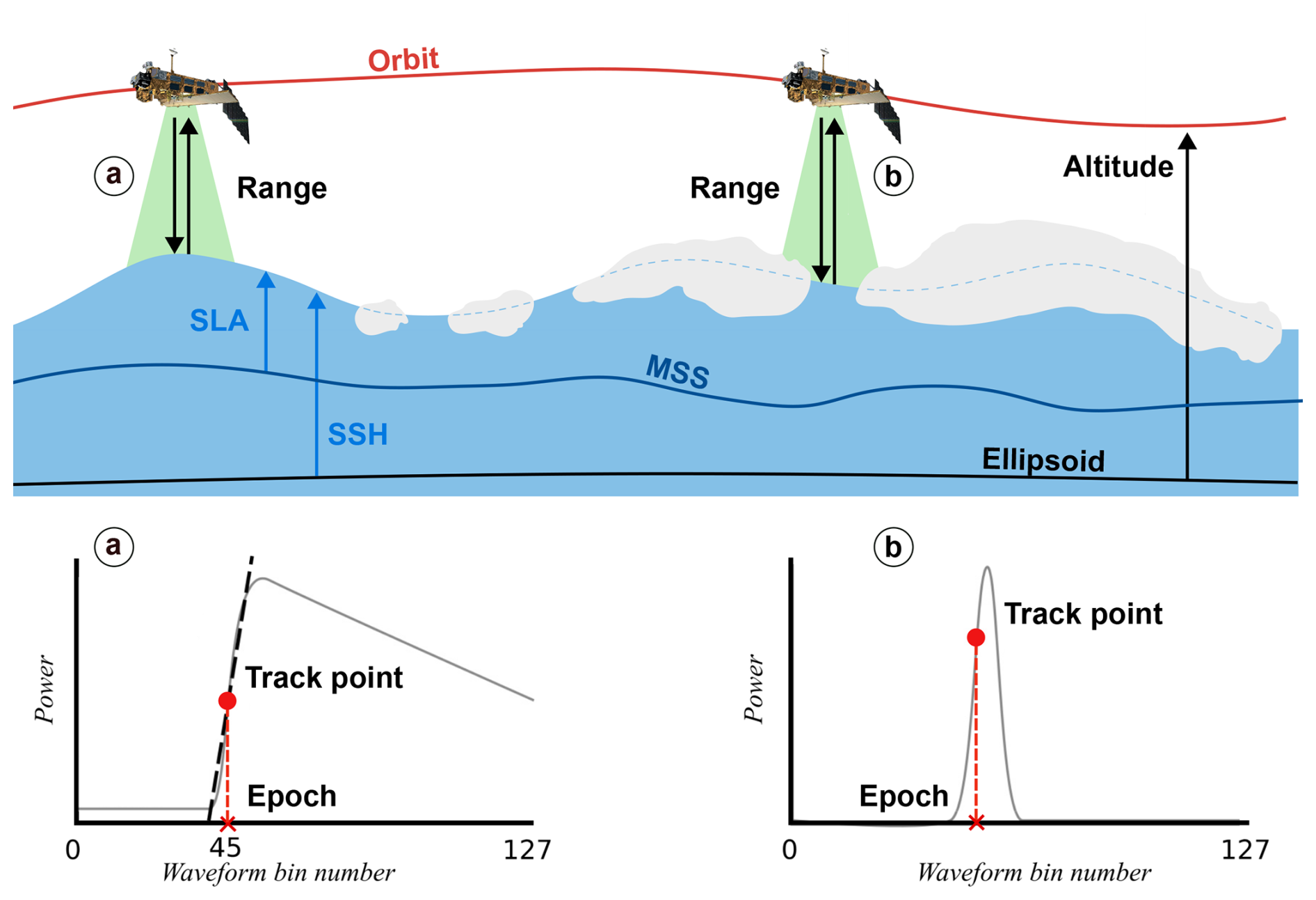
Figure 2 (a, top) Schematic of a satellite altimeter operating over the open ocean; (a, bottom) the corresponding radar echo (i.e. waveform) reflected by the open-ocean surface. (b, top) The same altimeter over sea ice, passing above a lead; (b, bottom) typical quasi-specular waveform reflected by a lead, with the epoch estimated by the retracking algorithm indicated by the red point.

2.2 Ancillary and validation data

Several independent datasets are used in this study for cross-calibration, validation, and comparison purposes.

2.2.1 C3S open ocean data

The Copernicus Climate Change Service (C3S) provides daily gridded SLA fields at 0.25° resolution, produced by integrating several missions with the DUACS processing system (Pujol et al., 2016; Taburet et al., 2019). Compared to SO_SLICE, it uses the same interpolation methodology but does not include observations within the sea-ice cover. As it is a reference in the community, it is used to validate the SO_SLICE processing pipeline in the open ocean and showcase its added value at high latitudes. The version used is the vDT2024 (Copernicus Climate Change Service, Climate Data Store, 2018).

2.2.2 Other altimetry datasets covering the ice-covered regions

Two other altimetric SLA products covering the ice-covered Southern Ocean are used for intercomparison. Dragomir (2024) is an SSH dataset spanning 2003–2018 that combines Envisat and CryoSat-2 data, though the record relies on a single mission for most of its duration (Envisat only before 2010, CryoSat-2 only after 2012). Auger et al. (2022a) produced a multi-mission product spanning 2013–2019 by combining CryoSat-2, SARAL, and Sentinel-3A. Comparing with both allows for the evaluation of SO_SLICE in ice-covered regions where C3S is not always available (Sect. 4.3.5).

2.2.3 In situ data

Two types of in situ observations are used for validation: tide gauges and bottom pressure recorders (BPRs). All platforms presented here were deployed in ocean regions with a seasonal or permanent sea-ice cover. Hourly tide gauge records from stations on the Antarctic coast are taken from the Gloss/Clivar dataset (IOC, 2012). They have been corrected for Dynamical Atmospheric Correction (Carrère and Lyard, 2003), ocean tide (Carrère et al., 2022) and glacial isostatic adjustment (Peltier, 2004). BPRs record pressure at the seafloor, providing a proxy for the variations of the ocean mass above the instrument. Six BPRs are used. Four are in the Drake Passage – referred to as Drake Passage South (DPS), Drake Passage South Deep (DPS Deep), Myrtle B and Myrtle C (PSMSL, 2024). The other two are ANT-17.1, deployed on the Greenwich meridian (Androsov et al., 2020), and the JARE BPR, deployed near Syowa station (Hayakawa et al., 2012). Deployment dates, geographic coordinates, and distance to coast are specified in Table S1 in the Supplement, and locations are shown in Fig. 10a.

3 Methods

To retrieve SLA, the standard altimetric processing described in Sect. 2.1 assumes the radar signal is reflected by the ocean surface, as in Fig. 2a configuration. This assumption breaks down in ice-covered regions. The altimeter footprint is predominantly occupied by sea ice. Measuring SLA in these conditions requires identifying locations where the ocean surface is directly visible, i.e. leads, and applying dedicated waveform retracking to estimate the associated range and SLA. This section describes the processing steps that allow SO_SLICE to integrate SLA measurements in ice-covered conditions. Figure 3 recapitulates the whole data pipeline.

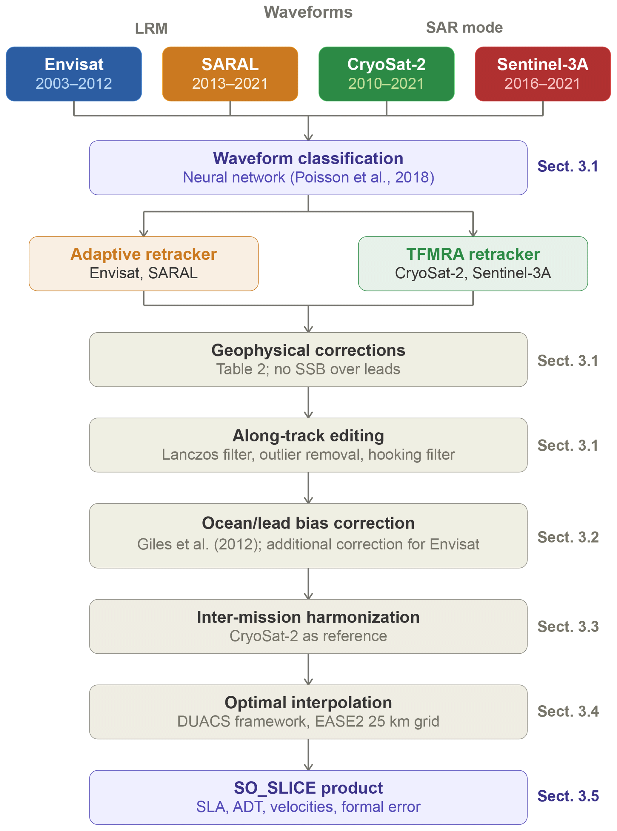
Figure 3 Data processing pipeline of SO_SLICE, from the input waveforms to the final gridded product. Each key step has its associated box and is discussed in the indicated subsection.

3.1 Lead detection, retracking and editing

The first step of the processing chain is to identify which measurements acquired within the ice-covered regions correspond to leads rather than ice. As the ocean within leads is sheltered from winds and waves, its surface is extremely smooth and acts as a quasi-specular reflector for the radar pulse. Thus, leads produce highly peaked returns associated with high backscattering coefficients. Lead signatures dominate the waveform, even if they cover a small fraction of the footprint (Drinkwater, 1991). This configuration is shown in Fig. 2b. Based on this property, a neural-network classifier (Longépé et al., 2019; Poisson et al., 2018) is used to automatically identify lead waveforms and discard sea-ice returns. The classifier categorizes each waveform into one of sixteen classes according to its shape. Lead echoes have their dedicated class. This neural-network classification is complemented by a multiple-criteria classification based on thresholds applied to waveform parameters, following Poisson et al. (2018).

Once a waveform is classified as a lead waveform, a retracking algorithm is applied to derive the range. For CryoSat-2 and Sentinel-3A, which operate in SAR mode above sea ice, the TFMRA empirical retracker is applied on lead waveforms (Helm et al., 2014). For their open ocean waveforms, a different retracker, MLE4 (Thibaut et al., 2010), is used. Sentinel-3A open ocean SAR waveforms are converted to pseudo LRM waveforms, to make the use of MLE4 possible. For the LRM missions, Envisat and SARAL, the Adaptive retracker (Poisson et al., 2018; Tourain et al., 2021) handles both open-ocean and lead waveforms within a single physical model. In all cases an offset between open-ocean and lead SLA remains: by construction for the SAR missions, which use two different retrackers, and as a residual for the Adaptive retracker, which reduces the offset by about 50 cm without eliminating it. This offset is corrected in Sect. 3.2.

The altimetric equation (1) is then applied to retrieve the SLA, with the same set of geophysical corrections and MSS as for the open ocean (Table 2). The only difference is that Sea State Bias (SSB) is not corrected for, under the assumption that wind and wave effects on the SSB are negligible in the ice-covered domain. This hypothesis should hold except in the marginal ice zone. Sea ice inhibits wave propagation coming from the open ocean (Squire, 2020), and protects surface water from wind generated ripples. While high frequency waves are efficiently dissipated by sea ice, low frequency waves can propagate within the sea-ice cover and may be a source of bias to our product. Unfortunately, no reliable SSB estimates currently exist for specular waveforms. SSB is empirically derived from significant wave height (SWH) and wind speed (Tran et al., 2010), but SWH is not reliably retrieved from specular lead waveforms (Poisson et al., 2018). Hence, all existing polar altimetric SLA products similarly neglect SSB in the ice-covered domain (e.g., Armitage et al., 2016; Auger et al., 2022a).

After classification and retracking, the along-track SLA records still contain outliers. A series of editing steps is used to remove them. This editing is consistent across all four missions and similar to the one applied in Auger et al. (2022a) and Veillard et al. (2024). An iterative editing is applied to the open ocean data only. Along-track SLA are filtered with a 124-point low-pass Lanczos filter, and outliers are determined as points such that $|\mathrm{SLA}-{\mathrm{SLA}}_{\mathrm{filtered}}|>\mathrm{2}\cdot \mathrm{SD}(\mathrm{SLA}-{\mathrm{SLA}}_{\mathrm{filtered}})$. This process is iterated until outliers represent less than 0.1 % of the measurement points. Then, a dedicated filter following Poisson et al. (2018) is applied to lead data to mitigate the off-nadir hooking (or snagging) effect. As leads are highly specular and associated with a high backscatter coefficient, their returns can dominate the waveform even when the lead is located off-nadir but within the beam-limited footprint. In such cases, the measured range is longer than the true nadir range, introducing a negative bias in the estimated SLA (Armitage and Davidson, 2014; Quartly et al., 2019). This correction is only applied to the LRM altimeters (mounted on Envisat and SARAL) as altimeters operating in SAR mode are much less affected by the hooking effect due to their smaller footprint.

Figure S3 in the Supplement shows the number of lead measurements per 100 km × 100 km × 1-month bin before and after editing. For Envisat, the median number of lead observations per bin decreases from approximately 300 to 35 after editing, with similar values for SARAL. The hooking filter accounts for the largest fraction of removed points, making the editing particularly conservative for the LRM altimeters. This filter is not applied to CryoSat-2 and Sentinel-3A, which consequently retain a higher fraction of lead measurements, at around 200 observations per bin after editing. Despite this substantial reduction for LRM missions, the remaining lead observation density is comparable to the open-ocean observation density or higher in the case of SAR altimeters. This is because the open-ocean along-track data are down-sampled from their native high-rate posting to 5 Hz (∼ 1.3 km along-track spacing) prior to interpolation. This down-sampling, applied after the editing described above, reduces the computational cost of the optimal interpolation while retaining scales well below the correlation length scales used in the mapping (Sect. 3.4). Lead observations are kept at their native posting to preserve the sampling density in the ice-covered domain.

3.2 Ocean/Leads bias correction

As described in Sect. 3.1, an offset between open-ocean and lead SLA remains for all four missions. To address this, we apply the ocean/lead (O/L) bias correction introduced by Giles et al. (2012). For each mission, SLA estimates from the two surface types are averaged into separate 75 km × 75 km × 10 d bins. The difference in SLA between the two types of surfaces is computed for each bin, then spatially averaged to obtain a monthly climatology of the O/L bias, which is interpolated to daily resolution and subtracted from the lead data. Applying the same correction to all four missions improves inter-mission consistency and leaves a white-noise-like bias (Fig. S1). For Envisat, however, a spatially heterogeneous bias remains, producing large negative anomalies at the ice edge. This residual bias varies linearly with waveform peakiness (the ratio of maximum to mean waveform power, a measure of specularity). We apply an additional correction equal to the peakiness times the slope of the regression between O/L bias and peakiness. This suppresses the negative anomalies and reduces the heterogeneous bias to a homogeneous one (Fig. S2).

3.3 Merging the missions

After correcting for the O/L bias of each individual mission, a cross-calibration is performed to account for inter-satellite offsets arising from differences in instruments, orbits and processing. CryoSat-2 is used as the reference mission as it overlaps with all three other missions. The strategy is analogous to the O/L bias correction. SLA estimates are aggregated in 75 km × 75 km × 10 d bins for each mission, and the mean offset relative to CryoSat-2 is computed over the overlapping time periods. These offsets are removed from each mission.

3.4 Optimal interpolation and gridding

After calibration, along-track data from all missions are combined into a daily gridded dataset using the DUACS mapping procedure (Taburet et al., 2019). It relies on an Optimal Interpolation algorithm (Bretherton et al., 1976; Ducet et al., 2000; Le Traon et al., 1998). SLA at each grid point is estimated as a weighted linear combination of nearby observations. The weights are determined by a space-time covariance function, which is controlled by three inputs: the spatial and temporal correlation scales, the expected signal variance, and the measurement noise. The correlation scales define the space-time radius within which the observations contribute to the grid point estimate. They thus control the smoothness of the output and the resolved scales. The signal variance sets the expected amplitude of SLA variability. The noise variance determines how much the optimal interpolation weights individual observations. In the absence of any nearby observations, the interpolation returns an SLA equal to 0 with an uncertainty equal to the full signal variance. SO_SLICE uses the inputs derived in Auger et al. (2022a), which are presented in Figs. S4 and S5. The spatial correlation scales range from 100 km in the ACC to 100–250 km in the subpolar Southern Ocean. The temporal correlation scales range from 30 d in the ACC to 10 d in the subpolar Southern Ocean. These parameters set a lower bound on the effective resolution of the gridded product. The effective spatial and temporal resolution of SO_SLICE are assessed in Sect. 4.3. The final output is distributed on an EASE2 polar stereographic grid (Brodzik et al., 2012), with uniform 25 km × 25 km spatial grid cells, centered on the South Pole. Monthly and daily files are available.

3.5 Available variables

In addition to the gridded SLA fields, several variables are derived and distributed alongside the product, for user convenience. They are listed in Table 3. First the Absolute Dynamic Topography (ADT) is provided, computed as:

$$\begin{array}{}\text{(3)}& \mathrm{ADT}=\mathrm{SLA}+\mathrm{MDT}\end{array}$$

The MDT used is from Jousset et al. (2026), derived from the CNES_CLS22 MSS (Schaeffer et al., 2023) and the GOCO06s (Kvas et al., 2021). As the MSS used for the MDT computation differs from the Hybrid MSS (Laloue et al., 2025) used for the SLA computation, a static residual between the two MSS products may be present in the ADT field. Thus, users must use this field with caution. Future versions of the product will use a consistent MSS for both the SLA and MDT computations. Surface geostrophic velocities are computed from the ADT field using:

$$\begin{array}{}\text{(4)}& {\mathit{u}}_g={\displaystyle \frac{g}{f}}\left(\widehat{k}\times {\mathrm{\nabla }}_{\mathrm{H}}\mathrm{ADT}\right)\end{array}$$

where g is gravity, f is the Coriolis parameter, $\widehat{k}$ is the unit vector normal to the geoid and ∇_H the horizontal gradient operator. These derived variables are provided for user convenience but are not analysed further in this study. The optimal interpolation also provides a formal mapping error at each grid point and time step, with the formula:

$$\begin{array}{}\text{(5)}& {\mathit{\sigma }}_{\mathrm{map}}^{\mathrm{2}}\left(x_{\mathrm{0}}\right)={\mathit{\sigma }}_{\mathrm{s}}^{\mathrm{2}}\left(x_{\mathrm{0}}\right)-c^{\mathrm{T}}{A}^{-\mathrm{1}}c\end{array}$$

where c is the vector of signal covariances between the target grid point x₀ and the surrounding observations, $A=C_s+R$ is the sum of the inter-observation signal covariance and the observational noise covariance, and ${\mathit{\sigma }}_{\mathrm{s}}^{\mathrm{2}}\left(x_{\mathrm{0}}\right)$ is the prior signal variance at x₀. Hence, it can be defined as the prior signal variance minus the variance reduction achieved by the observations (Bretherton et al., 1976). It reflects the residual signal variance left unexplained by the observations after optimal interpolation and is driven by the density and distribution of nearby observations. It does not account for systematic error sources such as residual biases or the omission of the SSB correction over leads. It should therefore be interpreted as a lower bound on the total uncertainty and is also distributed with the SLA field.

Table 3 Available datasets and associated fields.

4 Results

4.1 Along track SLA data

Figure 4 shows an example of along-track SLA measurements (Fig. 4a) used to produce SO_SLICE. They originate from an Envisat pass over the Weddell Sea (Fig. 4b) on 11 October 2003. The thin gray line shows the SLA estimates before editing, from both open-ocean and lead waveforms. After the processing pipeline, the retained measurements are shown in blue (open ocean) and red (leads). 85 % of the categorized open ocean waveforms are kept, and 10.5 % of the lead waveforms. The resulting 178 lead measurements provide SLA information in the ice-covered domain. The along-track profile illustrates the continuity between the two surface types: SLA evolves smoothly from the open ocean into the sea-ice sector, with no jump at the ice edge.

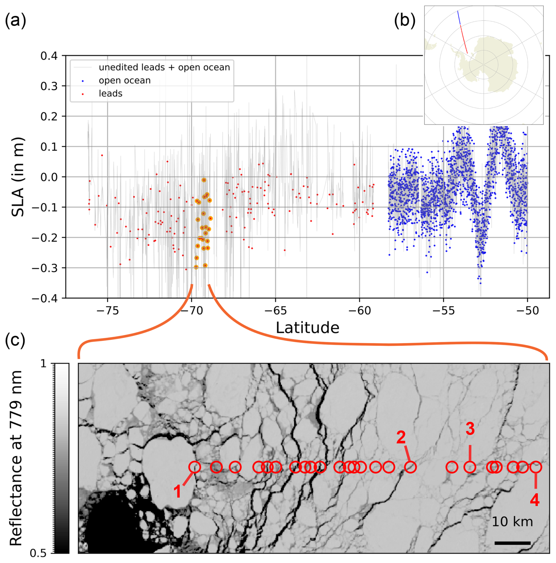
Figure 4 (a) SLA from one Envisat pass, on 11 October 2003. Blue points are edited SLA from open-ocean waveforms. Red points are edited SLA from lead waveforms. The gray line aggregates SLA estimates from open-ocean or lead waveforms, before the editing. (b) Trajectory of the along-track data shown in (a). (c) Surface reflectance at 779 nm along the trajectory, measured by MERIS. SLA estimates shown in orange in panel a are collocated on the MERIS swath. Points labelled 1 to 4 are discussed in the text.

To qualitatively illustrate that the retained lead points correspond to actual openings in the ice cover, we use the Medium Resolution Imaging Spectrometer (MERIS; Rast et al., 1999), also mounted on Envisat. MERIS measures the radiance at the top of the atmosphere at several wavelengths, with a spatial resolution of 300 m. During clear-sky periods, it distinguishes highly reflective surfaces (sea ice) from poorly reflective ones (open water). A subset of along-track lead points (highlighted in orange) is collocated on the MERIS swath (Fig. 4c). A small number of points illustrate residual limitations of the classification. Observation 3 is classified as a lead but overlies a surface with a reflectance intermediate between neighbouring leads and ice floes. It may be a lead not visible due to MERIS resolution, but could also correspond to newly formed sea ice whose flat and snow-free surface produces a quasi-specular echo similar to a lead (Drinkwater, 1991). Observation 4 is located above sea ice, with a lead visible slightly off-nadir in the cross-track direction. These cross-track contaminations are not systematically detected by the hooking filter introduced in Sect. 3.1. Such misclassifications are discussed in detail by Poisson et al. (2018). However, the majority of retained lead points, as illustrated by observations 1 and 2, coincide with low-reflectance surfaces at 779 nm corresponding to open water exposed in leads. These cases represent the bulk of the retained observations in this example. The gridded product validation presented in Sect. 4.3 provides an integrated assessment of the impact of residual classification errors on the final fields.

4.2 Final dataset

The along-track measurements from the four satellite missions are combined using the DUACS procedure described in Sect. 3.4. The resulting gridded SLA dataset, SO_SLICE, has a grid resolution of 25 km and covers the period 2003–2021.

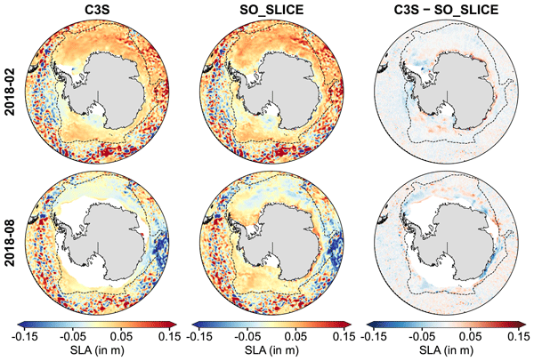
Figure 5 Monthly SLA fields relative to the 2003–2021 period from (a) C3S and (b) SO_SLICE, and (c) the difference between C3S and SO_SLICE. Each row corresponds to a specific month, from top to bottom: February 2008, August 2008, February 2018 and August 2018.

Figure 5 presents monthly SLA fields for February and August 2008 and 2018, from C3S (Fig. 5a) and SO_SLICE (Fig. 5b). Two regions are considered: the ACC region and the subpolar Southern Ocean, separated by the −1.05 m MDT contour from MDT_CNES/CLS22. In the ACC, the two products agree closely. Qualitatively, similar mesoscale patterns are visible in the monthly snapshots. Quantitatively, 95 % of grid points located in the ACC display a correlation greater than 0.80 between SO_SLICE and C3S. The residual differences of approximately 1 cm may reflect additional filtering applied to the open-ocean along-track data in C3S. In the subpolar region, the C3S SLA field is heavily smoothed and contains missing data under sea ice, whereas SO_SLICE provides SLA estimates year-round and across the entire region. It also resolves mesoscale features within ice-covered areas such as the Weddell Sea. The snapshots show no sharp frontier at the transition between open-ocean and sea-ice sectors, providing confidence in our processing and calibration. Where C3S does have data in the subpolar Southern Ocean, differences are larger than in the ACC. This arises from the climatological mean used to define the anomalies. For C3S, it is computed without wintertime observations in ice-covered regions, which biases the reference period. SO_SLICE, by contrast, includes observations from all seasons yielding a different and more representative climatology.

Figure 6 (a) Spatial PSD of SO_SLICE and C3S SLA fields in the ACC region and the subpolar Southern Ocean, as well as the ratio between SO_SLICE and C3S PSD. The linear fit between 250 and 70 km is plotted, and the associated slope is given in the legend. (b) Temporal PSD of SO_SLICE and C3S in the ACC and the subpolar Southern Ocean, with the PSD ratio for each region.

Figure 6a shows the spatial power spectral density (PSD) of SO_SLICE and C3S. To compute the spectra, the SLA field is divided into 1600 km × 1600 km patches. The isotropic PSD is computed in each patch, averaged over all directions and then averaged separately over patches of the ACC and of the subpolar Southern Ocean. In the ACC, both products agree closely at wavelengths longer than 150 km. The spectral slope close to k⁻⁵ is consistent with interior quasi-geostrophic dynamics expected in an eddy-rich region. At shorter wavelengths, SO_SLICE retains slightly more energy. This reflects the additional along-track filtering performed in C3S, which suppresses energy and noise at small scales. In the subpolar Southern Ocean, SO_SLICE contains substantially more energy at all wavelengths. The PSD ratio between the two products ranges from 5 at 1000 km to 17 at 50 km, illustrating the gain in resolved variability in ice-covered regions. This confirms that SO_SLICE and C3S resolve similar spatial scales in the ACC, and that SO_SLICE provides substantial added value in the subpolar Southern Ocean. Figure 6b shows the temporal PSD. In the ACC, both products are in close agreement at periods longer than 90 d, confirming the consistency of SO_SLICE with C3S for seasonal and interannual variability. At shorter periods (90–20 d), SO_SLICE retains slightly more energy, which we again attribute to differences in filtering. In the subpolar Southern Ocean, SO_SLICE spectrum closely matches its ACC counterpart, indicating that the datasets capture comparable levels of temporal variability in both regions.

4.3 Validation

The validation of SO_SLICE proceeds in five steps, progressing from the raw input data to the final gridded product. First, we assess the consistency of the along-track observations between missions before any interpolation is applied (Sect. 4.3.1). Second, we evaluate the quality of the interpolated maps by comparing maps in the ACC region and the subpolar Southern Ocean with independent satellite observations (Sect. 4.3.2). Third, we examine the formal error output by the optimal interpolation as a measure of internal uncertainty (Sect. 4.3.3). Fourth, we compare the product with independent in situ observations from tide gauges and bottom pressure recorders (Sect. 4.3.4). Finally, we assess the consistency of SO_SLICE with existing altimetric SLA products in the ice-covered Southern Ocean (Sect. 4.3.5).

4.3.1 Consistency between missions

As a first validation step, we compare the fully edited and calibrated outputs of each altimetry mission against one another. Each mission has different instrument characteristics, footprints and independent processing chains. A high level of agreement between them is therefore a strong indicator that the observed signal is geophysical rather than instrumental noise. For this comparison, SLA observations from each mission are averaged onto a 75 km EASE2 grid in 10 d bins, without optimal interpolation. Four sets of maps are obtained, one per mission. They are compared pairwise, using CryoSat-2 as the reference due to its temporal overlap with the three other satellites.

Figure 7 For each satellite mission, observations are binned onto the EASE2 75 km grid, with a 10 d time step. No optimal interpolation is used here. The resulting maps are compared between mission pairs. (a) Spatial spectral coherence for each pair of 75 km maps with a 10 d time step. (b, c, d) SLA spatially averaged over the subpolar Southern Ocean, compared between overlapping mission pairs (b: CryoSat-2 vs. Envisat, c: CryoSat-2 vs. SARAL, d: CryoSat-2 vs. Sentinel-3A). (e, f, g) Probability density of grid-point temporal correlations for each mission pair, on maps coarsened to 300 km per 300 km. The distribution is split between the ACC region and the subpolar Southern Ocean, as in Fig. 6. Median values are indicated by dashed lines. (h, i, j) Same as (e, f, g) but for the RMSD, in centimeters.

Figure 7a shows the spatial spectral coherence computed from these maps. As for the PSD analysis in Sect. 4.2, coherence is computed on 1600 km × 1600 km patches and averaged separately in the ACC and the subpolar Southern Ocean. The coherence γ²(k) measures the fraction of variance at each wavelength that is shared between two fields: γ²=1 indicates perfect agreement, while γ²<0.5 means that more than half the variance at that scale is independent between the two missions. For the two regions, all map pairs display coherence greater than 0.5 at wavelengths longer than 300 km, confirming that the satellites observe the same signal at these scales. This is corroborated by the time series of spatially averaged SLA in the subpolar Southern Ocean (Fig. 7b, c, d), which show strong mutual consistency at a 10 d time step. The Pearson correlation coefficient (r) and RMSD relative to CryoSat-2 are r=0.83 and RMSD = 1.18 cm for Envisat, r=0.93 and RMSD = 0.75 cm for SARAL, and r=0.87 and RMSD = 0.87 cm for Sentinel-3A.

At shorter wavelengths, the scale at which coherence drops below 0.5 depends on both region and instrument type. In the ACC, all pairs cross the 0.5 threshold at approximately 180 km, indicating that the maps agree down to similar scales in the open ocean. In the subpolar Southern Ocean, the coherence between CryoSat-2 and Envisat falls below 0.5 at 304 km, and between CryoSat-2 and SARAL at 247 km, indicating weaker agreement than in the ACC. Several factors contribute to this degradation. LRM altimeters have higher measurement noise than SAR instruments (Boy et al., 2017), which reduces the signal-to-noise ratio at short wavelengths. In addition, the sparser sampling density of the LRM missions increases the likelihood that they observe a given grid cell at different times than CryoSat-2 within a 10 d window. This introduces temporal representativeness errors that appear as decorrelation. By contrast, maps from CryoSat-2 and Sentinel-3A, the two SAR altimeters, maintain a similar coherence threshold in both regions. The higher sampling density of these missions produces more consistent measurements over leads, sustaining agreement to shorter wavelengths even under ice.

To complement the spectral analysis, the right-hand panels of Fig. 7 show grid-point RMSD and correlation distributions for each pair. These are computed on maps now coarsened to a 300 km grid, the scale above which all pairs show coherence greater than 0.5. For CryoSat-2 vs. Envisat, the RMSD and correlation distributions are similar in the ACC and the subpolar Southern Ocean, with median RMSD above 3 cm and median correlation of 0.64 in both regions. For the other two pairs (CryoSat-2 vs. SARAL, CryoSat-2 vs. Sentinel-3A), median RMSD values are lower (∼ 1.8–1.9 cm) and median correlations are higher (∼ 0.8 in the subpolar Southern Ocean, ∼ 0.9 in the ACC), consistent with the lower range noise of SAR (Boy et al., 2017) and Ka-band (Verron et al., 2021) altimeters. Together, these diagnostics confirm robust inter-mission agreement at scales larger than 300 km across the entire domain. At smaller scales, the disagreement is driven by instrumental noise and spatially heterogeneous sampling. These limitations reflect the properties of the raw binned maps (75 km grid, 10 d time step) before any interpolation is applied. Merging multiple missions through the optimal interpolation is expected to mitigate them by increasing the effective observation density with correlation length scales larger than 75 km.

4.3.2 Mapping in the ACC vs. the subpolar Southern Ocean

The previous section confirmed that the missions measure the same signal at scales larger than 180 to 300 km, validating the input data. We now evaluate the interpolated maps, the product delivered to users, with the aim of testing whether the mapping performs as well in the subpolar Southern Ocean as in the ACC. Since our open-ocean reconstruction closely matches the well-characterized C3S dataset (Sect. 4.2), the ACC serves as a benchmark against which the subpolar Southern Ocean can be evaluated. In practice, along-track SLA from a given altimetry mission are compared with interpolated SLA fields generated from the other missions, for the five available mission combinations. Along-track SLA observations are first smoothed with a 15 km running mean to reduce high frequency noise. The corresponding gridded SLA are interpolated onto the along-track positions and the pointwise differences (SLA_along-track−SLA_interpolated) are binned onto a 1° × 1° grid where RMSE values are computed. This RMSE is not a comprehensive uncertainty estimate, but it provides a practical measure of how well the maps reproduce the signal seen by an independent altimeter in each region.

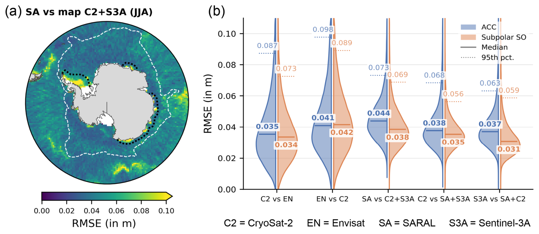
Figure 8 (a) Winter (June–July–August) RMSE map of SARAL along-track values compared to interpolated data from a CryoSat-2 + Sentinel-3A map, during the period 2016–2021. The white dotted line is the ACC/subpolar Southern Ocean MDT contour. The black dashed line is the 3 % contour of the climatological minimum of sea-ice concentration for 2016–2021. (b) Distribution of grid-cell RMSE for the five sets of along-track data/map comparison. ACC grid cells are in blue and subpolar Southern Ocean cells in orange. The median of the distribution is indicated by the thick full lines, with their associated values. The thin dotted lines are the 95 % percentile.

Figure 8 presents a winter (JJA) RMSE map from one leave-one-out comparison: SARAL along-track observations against CryoSat-2 + Sentinel-3A maps (Fig. 8a). The highest RMSE values, up to 10 cm, occur in the energetic regions of the ACC where intense mesoscale activity (Hughes and Ash, 2001) creates discrepancies between localized along-track observations and interpolated fields, especially when the mapped missions do not sample the region at the same time as the withheld altimeter. Elevated RMSE values are found in the permanently ice-covered regions (within the black dashed contour) such as in the Weddell Sea. This is due to higher retrieval uncertainties linked to artifacts in the MSS. Outside these regions, the RMSE is broadly consistent between the ACC and the subpolar Southern Ocean, as shown by the distributions in Fig. 8b. For SARAL vs. CryoSat-2 + Sentinel-3A, the median RMSE is 3.8 cm in the subpolar Southern Ocean and 4.4 cm in the ACC. The Envisat vs. CryoSat-2 comparison yields similar median values, but with a wider distribution (higher 95th percentiles and lower 5th percentiles in both regions). This reflects the role of multi-mission sampling. Maps constructed from two missions have denser spatial coverage, which on average reduces the discrepancy with the withheld altimeter. However, if only one of the two mapped missions samples a region at the same time as the reference, the interpolation blends synchronous and non-synchronous observations, introducing a representativeness error absent from single-mission maps. The net effect is a more compact RMSE distribution with a similar median. Similar RMSE values are obtained for the other mission combinations, with typical median RMSE values around 4 cm, and a slight tendency toward lower RMSE in the subpolar Southern Ocean (Fig. 8b). These leave-one-out values are upper bounds on the errors of the final product, which integrates all four missions rather than withholding one. Overall, the comparable RMSE values in the two regions indicate that the mapping of lead returns in the seasonally ice-covered subpolar Southern Ocean achieves a quality comparable to the open-ocean mapping in the ACC.

4.3.3 Formal error

The formal mapping error of the optimal interpolation (Sect. 3.5) is used here as a proxy for the local uncertainty of the reconstructed SLA field. Figure 9 presents daily maps of this formal error under different satellite observation scenarios. Figure 9a corresponds to a day in August 2008, during which only Envisat data are used. The average formal error at that time is 1.7 cm, with higher uncertainty concentrated within highly energetic regions of the ACC, the marginal ice zone, and certain coastal areas. Banded patterns stem from the uneven distribution of satellite tracks. Overall, uncertainty hotspots reflect the combined effects of lower observation density, stronger mesoscale activity, and signal aliasing due to the limitations of a single-mission dataset. Panel (b) of Fig. 9 illustrates the formal mapping error for a day in 2012 when only CryoSat-2 data are available. Despite the improved precision of its SAR mode over leads compared to Envisat (Sect. 2.1), having only CryoSat-2 SAR data has two intrinsic limitations for lead SLA mapping. Its SAR mode acquisition does not extend close to the coast in many regions, and its orbit results in daily maps with spatial gaps. These limitations manifest as increased domain averaged formal errors (south of 50° S), with pronounced striping artifacts and degraded confidence near the coast, visible both in the map (Fig. 9b) and the time series (Fig. 9e). Panel (c) of Fig. 9 illustrates the formal error on a representative day in August 2018 when the multi-mission dataset includes CryoSat-2, SARAL, and Sentinel-3A. The incorporation of multiple satellite tracks improves spatial sampling and cross-track resolution, leading to a reduction in the average formal error to 1.1 cm. Although the same dynamical regions (ACC, marginal ice zone, and coastal zones) remain areas of enhanced uncertainty, the magnitude of these errors is significantly lower. This highlights the main benefit of combining several missions. It reduces the uncertainty of SLA estimates, especially in higher uncertainty regions.

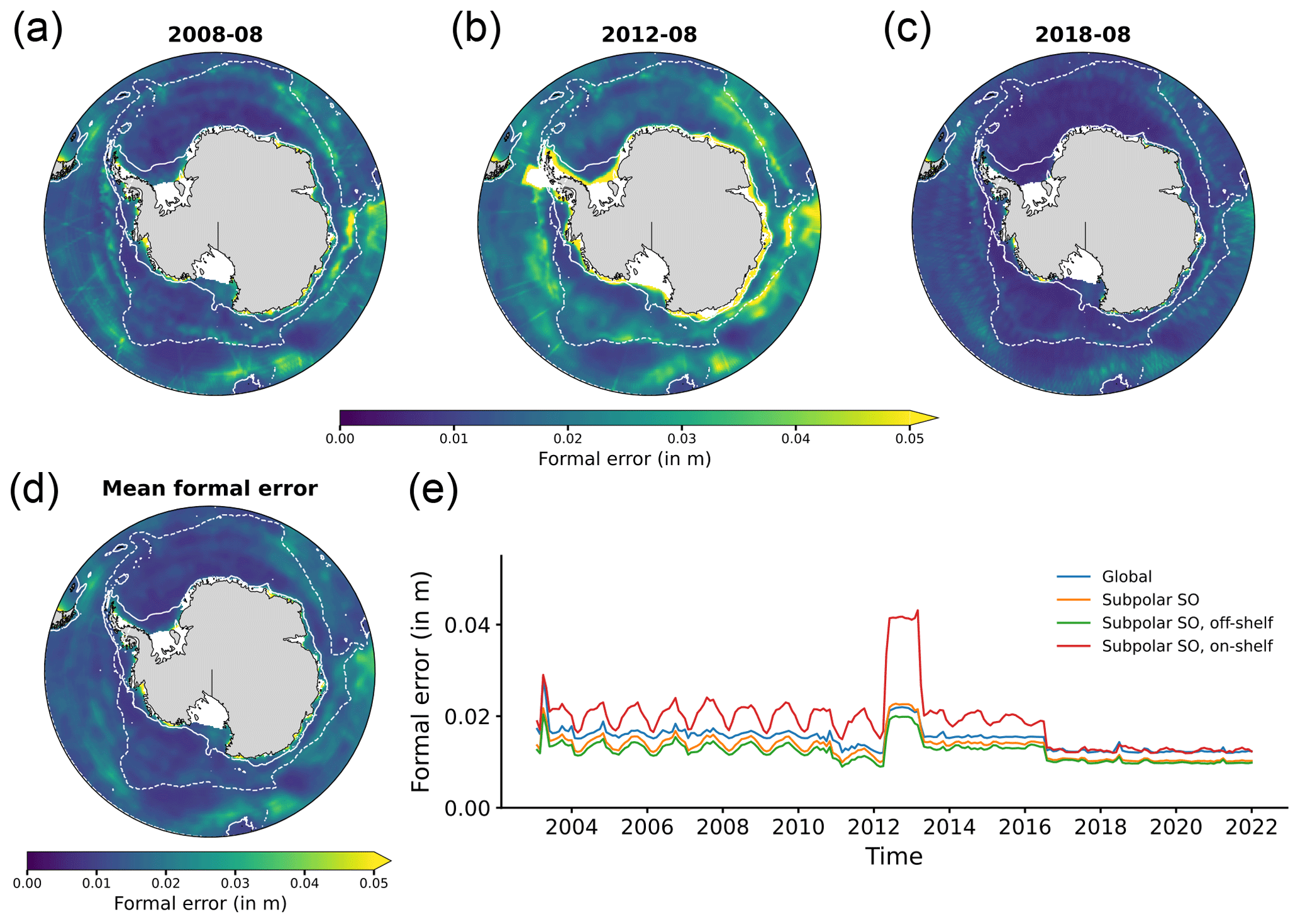
Figure 9 Daily formal error maps for one August day in (a) 2008 (Envisat only), (b) 2012 (CryoSat-2 only) and (c) 2018 (CryoSat-2, SARAL and Sentinel-3A). (d) Time-averaged daily formal error map over the full period. (e) Spatially averaged formal error time series, for several subdomains: south of 50° S in blue, subpolar Southern Ocean in orange, off-shelf subpolar Southern Ocean in green and on-shelf subpolar Southern Ocean in red. The subpolar Southern Ocean is south of the white dashed contour in the maps; the off-shelf/on-shelf separation is defined by the 1000 m bathymetric contour shown as a white full contour.

Overall, the formal error analysis gives a typical uncertainty of approximately 1.5 cm for SO_SLICE, in line with previous estimates by Armitage et al. (2016) or Giles et al. (2012). The subpolar Southern Ocean has an average uncertainty of 1.3 cm, with larger uncertainties on the continental shelf (average: 1.9 cm) than off the shelf (average: 1.2 cm). These are average numbers: the local uncertainty can be quite different as it is strongly affected by the density of observations, i.e. the number of satellites available and their orbit (Fig. 9e). The formal error time series also highlights the benefits of multi-mission merging. During the Envisat-only period (2003–2010), the subpolar formal error displays a seasonal cycle, peaking at 1.9 cm in winter when ice coverage is at its maximum and sampling density is at its lowest. From 2013 onward, the addition of SARAL and Sentinel-3A largely suppresses this seasonality and reduces the peak formal error to 1.1 cm in the subpolar Southern Ocean. We note that the formal error does not capture systematic errors, such as satellite-specific biases, retracking uncertainties, or residual geophysical corrections. As such, while the formal error maps are a valuable diagnostic, they must be interpreted as only one component of the total uncertainty.

4.3.4 Comparisons with in situ observations

SO_SLICE is compared with observations from in situ instruments. We use six tide gauges and six Bottom Pressure Recorders (BPRs) for this validation step (Fig. 10a). The majority of BPRs are located in the Atlantic sector of the subpolar Southern Ocean, while all tide gauges are deployed on the Antarctic coast, either in the Indian or Atlantic sector. There are several caveats to this comparison. First, the number of available instruments remains limited, reflecting the scarcity of sustained observational platforms in the Southern Ocean. Nevertheless, this study compiles the largest set of in situ records used for SLA validation in this region to date. Second, the spatial coverage is restricted to the Atlantic and Indian Ocean sectors, with no data available from the Pacific sector. Finally, the operational periods of the instruments primarily overlap with the first half of the altimetry record. It is the period with only Envisat, hence the one with the highest uncertainties (Fig. 9e).

Figure 10 (a) Locations of the in situ instruments (blue circles: tide gauges; red triangles: BPRs). (b) 15 d smoothed SLA time series from the Mawson tide gauge (blue) and the collocated SO_SLICE average within 150 km (orange); gray shading indicates sea-ice concentration > 10 % (EUMETSAT OSI SAF, 2017). (c) 2D histogram of SO_SLICE SLA vs. tide-gauge SLA for all data points with sea-ice concentration > 10 %, with the regression line (red) and the 1 : 1 line (dashed black). (d) Same as (b) for the Syowa tide gauge. (e) Same as (c) for the BPRs. (f) Same as (b) for the ANT-17.1 BPR, with an additional 60 d rolling average subtracted to isolate the 15–60 d variability band.

Despite these limitations, the comparison provides valuable insight into SO_SLICE performance. The observations are filtered to make a reliable comparison. For tide gauges, both the product and in situ time series are smoothed using a 15 d moving average. For BPRs, the 60 d rolling average is removed from the 15 d rolling average to isolate variability within the 15–60 d frequency band. Vinogradova et al. (2007) demonstrated with a modeling study that bottom pressure variations south of 60° S are significantly correlated to SLA on periods shorter than 60 d. In addition, SLA time series from the satellite-based dataset are spatially averaged within a 150 km radius of each in situ instrument. Correlations between the satellite-derived SLA and tide-gauge observations are all statistically significant (p≪0.05) with correlation coefficients ranging from 0.51 to 0.77 depending on the tide gauge (Table 4, Figs. S8–S13). Two examples of time series are shown in Fig. 10b, d to illustrate the good agreement including under sea-ice cover (gray shading on Fig. 10). We find correlation coefficients of 0.77 and 0.6 and RMSE values of 4.2 and 6.4 cm for the time series shown in panels (b) and (d), respectively. Seasonal cycles are well captured, although some discrepancies in amplitude are noted. Shorter-timescale variability (∼ 15 d) is also partially resolved by the product. A regression analysis aggregating all tide gauge data points during sea-ice conditions (> 10 % ice cover) yields a correlation of 0.58 and an RMSE of 4.8 cm (Fig. 10c). The regression deviates from the 1 : 1 line, with extreme SLA values being biased low in the satellite-derived product. The slope of the linear fit between the aggregated tide gauges and our altimeter product is 0.47. This may be attributed to several factors: the coastal proximity of tide gauges, where satellite altimetry performance is known to degrade; the temporal mismatch between satellite overpasses and short-lived coastal features; the smoothing and averaging applied to the product; and the uncertainty introduced by tidal aliasing and corrections in polar coastal regions. Similar to the comparison with the tide gauges, all correlations between satellite-based SLA and BPRs are statistically significant, with correlation coefficients ranging from 0.57 to 0.85 (Table 5; Figs. S14–S18). One example of time series shown in Fig. 10f demonstrates that SLA variability in the 15–60 d range is well captured, with a correlation of 0.52. A regression analysis combining all BPR data points yields a correlation of 0.66 and an RMSE of 1.1 cm for ice-covered periods (Fig. 10e). Similar to the tide gauge comparison, the regression slope deviates from the 1 : 1 line. SO_SLICE underestimates the largest local SLA values.

Table 4 Comparison metrics with tide gauges, computed with data points when sea-ice concentration is greater than 10 %. Effective temporal resolution as defined by Ballarotta et al. (2019).

Table 5 Comparison metrics with the full Bottom Pressure Recorders time series, computed with data points when sea-ice concentration is greater than 10 %. Effective temporal resolution as defined by Ballarotta et al. (2019).

Overall, this comparison between satellite-based SLA estimates and in situ observations confirms that the product reliably captures sub-seasonal SLA variability even in ice-affected regions, with an error of 1–5 cm and a tendency to underestimate SLA extremes. The largest errors (4–5 cm) come from the tide-gauge comparisons, which are all at coastal sites. Further away from the coast, error estimates computed from comparisons with BPRs drop to 1–2 cm.

4.3.5 Comparison with recent altimetry products

Figure 11a shows the spatial PSD of SO_SLICE compared to Dragomir (2024) and Auger et al. (2022a) over the ACC and subpolar Southern Ocean. Compared to Dragomir (2024), SO_SLICE contains more energy at all wavelengths except the very largest scales (> 1000 km), in both regions. It is consistent with the Dragomir product relying on a single mission for most of its record, which limits the observation density and thus the resolved variability. Its mapping procedure is a 1° × 1° spatial binning which acts as a low-pass filter and suppresses variability at a cutoff wavelength. SO_SLICE PSD agrees well with Auger et al. (2022a). In the ACC, Auger et al. displays slightly more energy at short wavelengths, possibly reflecting differences in along-track editing or noise levels. In the subpolar Southern Ocean, the two spectra are in close agreement across most scales. Gridded maps of pointwise RMSD and correlation between SO_SLICE and the two products are shown in Fig. 11b and c. The associated boxplots can be found in Fig. S7. Once again, the ACC is where the differences with Dragomir (weak correlation, large RMSD) are the most striking. In the subpolar Southern Ocean, the median RMSD is at 2 cm in both cases. The temporal correlation is 0.8 with Auger et al. (2022a) and 0.7 with Dragomir (2024). The higher correlation with Auger et al. is expected, as the two products share a similar processing methodology and common satellite missions over the 2013–2019 period. The main differences with Auger et al. (2022a) are concentrated on the continental shelf, particularly in the Weddell Sea. These are attributed to a change in MSS between the two products. The main differences with Dragomir are found near the coast and in the northernmost part of the subpolar Southern Ocean. The coastal discrepancies likely reflect the inclusion of CryoSat-2 SARIn data for Dragomir, while the northern boundary differences may arise from the different spatial extent and mission coverage of the two products. Overall, these comparisons confirm that SO_SLICE is consistent with existing independent products where they overlap, while offering extended temporal and spatial coverage.

Figure 11 (a) Spatial PSD of the SO_SLICE SLA field compared to the Dragomir (2024) and Auger et al. (2022a) datasets, computed separately in the ACC (left) and the subpolar Southern Ocean (centre). The right panel shows the ratio of the SO_SLICE PSD to each comparison product, for each region. (b) Grid-point correlation (left) and RMSD (right) maps between SO_SLICE and Dragomir (2024). (c) Same as (b) but between SO_SLICE and Auger et al. (2022a).

4.4 Effective resolution of SO_SLICE

After validating SO_SLICE, its effective spatial and temporal resolution is computed. The effective spatial resolution of a gridded altimetric product is the shortest wavelength at which the mapped fields faithfully represent the ocean signal. To estimate it, we follow the procedure of Ballarotta et al. (2019), who used the ratio of mapping-error spectrum to signal spectrum to characterize operational DUACS products. Independent along-track observations, i.e. measurements withheld from the interpolation (here one year of CryoSat-2 along-track data, see below), serve as ground truth. The mapping error is defined as the difference between these withheld measurements and the collocated gridded SO_SLICE values. The effective resolution is then the wavelength at which the noise-to-signal ratio (NSR), defined as the PSD of the mapping error divided by the PSD of the ground truth, crosses 0.5 when moving from large to small scale.

Figure 12 (a) SLA along one CryoSat-2 pass withheld from the optimal interpolation (black) and the collocated gridded SO_SLICE values (red); the orange and blue shadings indicate two 500 km segments used for the spectral analysis. (b) NSR spectra computed on the orange and blue segments of (a), and the mean NSR spectrum over all segments of this pass (black); the dashed line indicates the NSR = 0.5 threshold, and the resulting effective resolutions are given in the legend. (c) NSR spectra averaged over all segments within five latitude bands, and the associated effective resolutions. (d) Map of the effective spatial resolution, estimated from NSR spectra averaged within 10° × 10° bins.

The NSR is computed on 500 km segments extracted from one year of CryoSat-2 along-track data withheld from the mapping. Figure 12a shows an example along-track pass with two such segments. The orange segment lies mainly in the ACC, yielding an estimated effective resolution of 105 km. The blue segment is located in the subpolar Southern Ocean and consists of lead measurements. It yields an effective resolution of 184 km. As illustrated by this example, individual spectra are noisy. Obtaining robust estimates requires averaging over many segments to obtain stable NSR spectra. To do so and regionalize our metrics, each segment is referenced by its median latitude and spectra are averaged within latitude bands. Figure 12c shows the resulting NSR curves for several bands. From 50 to 65° S, the effective resolution lies between 124 and 138 km, consistent with both the input correlation scales prescribed in the interpolation (Sect. 3.4) and the values reported by Ballarotta et al. (2019) for the C3S product at comparable latitudes. South of 65° S, the effective resolution degrades to approximately 200 km, as observed for example in the Weddell Sea. This is consistent with the longer correlation scales prescribed in this region, and the sparser observation density that limits the amount of information the optimal interpolation can extract. Segments are also referenced by their longitude and binned in 10° × 10° boxes to produce the effective resolution map of Fig. 12d. Overall, the spatial pattern of effective resolution closely follows the input correlation length scales, with lower resolution found in the Weddell Sea and in the north of the Ross Sea, where the correlation scales are the highest. This points toward these parameters being the primary control on the resolved scales of the gridded product.

The effective temporal resolution is estimated using the same NSR framework. The in situ observations described in Sect. 4.3.4 serve as ground truth. The NSR is computed on 180 d segments between collocated SO_SLICE values and in situ records. Tables 4 and 5 summarize the temporal effective resolution estimated at each station, and the corresponding NSR spectra are provided in the Supplement. The estimated temporal resolution ranges from 23 to 48 d across stations, with a mean of 37 d. This is consistent with the temporal correlation scales prescribed in the Optimal Interpolation, which range from 20 to 30 d in the coastal subpolar Southern Ocean and the Drake Passage. It is also comparable to the average temporal resolution of 34 d estimated by Ballarotta et al. (2019) for the C3S product. In both studies, the temporal resolution estimate relies on comparison with in situ observations that are predominantly coastal. Altimetric performance is known to degrade near the coast due to land contamination of the radar footprint and less accurate geophysical corrections. The values reported here may therefore represent a conservative estimate of the temporal resolution in the offshore ocean, where these coastal effects are absent.

5 Data availability

The altimetry product discussed in this article is publicly available on Zenodo at: https://doi.org/10.5281/zenodo.17467407 (Mosneron Dupin et al., 2025).

6 Discussion

In this study, we presented SO_SLICE, a 19-year SLA dataset covering the open-ocean and ice-covered Southern Ocean over the period 2003–2021. It is the longest altimetric record currently available for the entire Southern Ocean. The approach relies on detecting radar echoes reflected from leads and extracting SLA measurements from them. Certain assumptions are required, most notably the omission of the SSB correction for sea-ice covered regions. They are known sources of residual bias. After editing, the density of valid observations in ice-covered regions is comparable to or greater than in the open ocean. Along-track data from four satellite altimetry missions are combined through optimal interpolation into gridded SLA fields on a 25 km EASE2 grid. The product provides spatially continuous coverage across the open-ocean and ice-covered domains, with smooth transitions at the ice edge, and its spectral content is consistent with the expected dynamical regimes in the ACC while revealing a substantial gain in resolved variability in the subpolar Southern Ocean compared to the C3S reference product.

The validation proceeds from the edited along-track data to the final gridded product. Cross-comparison of the binned, un-interpolated along-track data shows that all mission pairs observe the same geophysical signal at wavelengths longer than 300 km (Sect. 4.3.1). Leave-one-out comparisons yield median RMSE values of approximately 4 cm in both the ACC and the subpolar Southern Ocean, even during the Envisat-only period. This demonstrates that the lead-based retrievals constrain the interpolated fields in the ice-covered domain with an accuracy comparable to the open ocean (Sect. 4.3.2). The main benefit of merging several missions is a reduction of uncertainty, with the subpolar formal error decreasing from 1.9 cm (single mission) to 1.1 cm (multi-mission; Sect. 4.3.3). Comparison with fully independent in situ records (Sect. 4.3.4) yields statistically significant correlations, with mean coefficients of 0.58 for tide gauges and 0.66 for BPRs, confirming that the product captures sub-seasonal variability in ice-covered regions, including during the early, Envisat-only period. The main limitation is an underestimation of SLA extremes near the coast (regression slope of 0.47 against tide gauges), which we attribute to coastal processes unresolved by the product and to tidal-correction inaccuracies at these sites.

The effective spatial resolution of SO_SLICE is approximately 120 km between 50 and 65° S, similar to the C3S product at these latitudes (Ballarotta et al., 2019). It degrades to 200 km south of 65° S, with slightly coarser values obtained for the Envisat-only period (Fig. S19). The effective temporal resolution ranges from 23 to 48 d, with a mean of 37 d (Sect. 4.4). These values closely follow the correlation scales prescribed in the optimal interpolation, confirming that these parameters are the primary control on the resolved scales. The 25 km, daily gridded output may oversample the true information content of the product, and users should interpret the fields accordingly. In particular, Auger et al. (2023) identified mesoscale eddies under sea ice in a similar product; our analysis suggests that such features are only reliably resolved at wavelengths longer than approximately 200 km in the subpolar Southern Ocean, and smaller eddies should be interpreted with caution. SO_SLICE nevertheless resolves spatial and temporal scales that no other gridded altimetric product currently captures in the ice-covered Southern Ocean.

This dataset represents a significant step forward in observing sea level variability in the Southern Ocean, particularly in regions previously obscured by sea ice. With nearly two decades of consistent altimetry coverage across both open ocean and ice-covered areas, it offers new opportunities to investigate large-scale and mesoscale ocean dynamics, trend analysis, and interannual variability in sea level in the subpolar Southern Ocean. It can support studies of subpolar gyre variability (Dotto et al., 2018), Antarctic Bottom Water export, and ice-shelf–ocean interactions (Lauber et al., 2023), especially where other observing systems (in situ and other satellite observations) are limited. Further improvements are planned, such as the integration of additional satellite missions (Sentinel-3B, Sentinel-3C), and a tuning of the correlation scales to improve the final effective resolution. By extending the observational record and bridging the observational gap across the ice edge, SO_SLICE provides a valuable resource to better understand the physical processes at play in the Southern Ocean and how it has been changing over the past two decades.