Grounded icebergs around Antarctica: a high-resolution dataset derived from deep learning and Sentinel-1 synthetic aperture radar

Icebergs frequently run aground on shoals on the continental shelf around Antarctica. Once rendered immobile, they can anchor landfast sea ice (fast ice) and their supply of limiting trace nutrients contribute to driving coastal marine productivity. They are also associated with seabed scouring, with implications for benthic marine ecosystems. Despite their importance, there is currently a lack of accurate, continent-wide automated mapping of grounded iceberg distribution and size and as a consequence, no large-scale, complete map of grounded icebergs exists. To address these gaps, this study implements an automated grounded iceberg detection framework based on Sentinel-1 Synthetic Aperture Radar (SAR) imagery, integrating a proposed ResUNet deep-learning network with a multi-temporal identification algorithm, incorporating strict physical constraints derived from bathymetry and sea ice concentration to mitigate environmental false positives. The method demonstrates strong robustness against interference from complex coastal conditions, achieving a detection F1 score exceeding 0.91 and successfully reducing the minimum detectable iceberg size to 0.016 km². Since the presence of fast ice makes distinction between “truly grounded icebergs” and “those held motionless by fast ice”, we capitalise on the unprecedented low fast ice extent in early 2025 (late February to early April) to construct the first high-resolution, continent-wide dataset of grounded icebergs around Antarctica. A total of 39 619 stationary icebergs were identified on the Antarctic continental shelf. We partition these stationary targets into “high-confidence grounded icebergs” and fast ice-entrapped candidates. Analysis shows that 67.4 % of these targets are identified as high-confidence grounded. Across the entire dataset, tiny icebergs (<1 km²) dominate numerically, accounting for 92.6 % of the total. These high-density grounded iceberg clusters are primarily concentrated on shallow continental shelves and west of (i.e., downstream of) the actively disintegrating fronts of ice shelves, forming complex and discontinuous “grounded iceberg chains”. Our dataset reveals that these grounded icebergs cover a combined area of 13 430 km² and are widely distributed along 56.5 % of the Antarctic coastline, with just 14.2 % of the coastline containing 80 % of all grounded icebergs. Crucially, while typically overlooked, tiny icebergs (<1 km²) contribute 53.9 % of this total grounded area. These dense clusters imply a potential “picket fence effect”, acting as a series of physical anchors to stabilise fast ice. This provides a quantitative baseline for modelling fast ice stability, assessing nutrient fluxes, and mapping benthic habitats. The grounded iceberg dataset (Jiao et al., 2026) is available at https://doi.org/10.25959/54sx-pt47.

1 Introduction

Antarctic icebergs originate from the calving of ice shelves and tidewater glaciers, a fundamental process that regulates the mass balance of the Antarctic Ice Sheet (Rignot et al., 2013; Greene et al., 2022). The discharge of ice into the Southern Ocean is not merely a passive decay but a critical component of ice-sheet dynamics; recent assessments indicate that calving accounts for approximately half of the continent’s total mass loss, comparable to that of basal melting (Rignot et al., 2013; Greene et al., 2022). These calving events produce floating ice masses ranging from small fragments to massive tabular icebergs, which serve as proxies for ice-shelf break-up processes (Scambos et al., 2009). Importantly, these icebergs retain substantial subsurface drafts, typically spanning from tens of metres to depths exceeding 500 m (Dowdeswell and Bamber, 2007). It is this substantial keel depth that predisposes them to interact with the seafloor on shallow continental shelves, transforming them from drifting bodies into stationary grounded features.

Once detached from their parent ice shelves, icebergs drift across the Southern Ocean, driven by the complex interplay of wind stress, ocean currents, the Coriolis force, and sea ice dynamics (Gladstone et al., 2001; Bigg et al., 1997). More recent models also account for interactions between icebergs, sea ice, and wave radiation stress (e.g. Merino et al., 2016; Rackow et al., 2017), which are increasingly recognised as essential components in Earth System Models (Vancoppenolle et al., 2025). When these deep-draft icebergs drift across the Antarctic continental shelves, where water depths are often less than 500 m (Dorschel et al., 2022), their keels can contact the seabed (Dowdeswell and Bamber, 2007; Olivé Abelló et al., 2025). This interaction anchors drifting ice, establishing them as “grounded icebergs”, stationary features that can remain in place for periods ranging from days to several decades (Woodworth-Lynas et al., 1991; Leane and Maddison, 2018).

Grounded icebergs play a critical role in the Antarctic sea ice system, serving as key anchor points for Antarctic landfast sea ice (“fast ice”; Wright and Priestley, 1922), and together with fast and pack ice, ice shelves and coastline, they form a complex coastal ice–ocean interaction network (Porter-Smith et al., 2021; Fraser et al., 2023; Vancoppenolle et al., 2025). Grounded icebergs not only fix and stabilise fast ice, prolonging its residence and enhancing the continuity and spatial cohesion of coastal ice zones (Massom et al., 2001; Li et al., 2020; Fraser et al., 2023). Furthermore, they act as topographic barriers that impede the upstream advection of sea ice; by blocking external pack ice from entering, they allow offshore winds to clear the downstream (leeward) side of sea ice (e.g., see Fig. 11 in Fraser et al., 2023). This obstruction and alteration of ice distribution promotes polynya formation, the development of thick ice zones, and influence the intrusion of warm currents and ice shelf melting (Nakayama et al., 2014; Fraser et al., 2019; Bett et al., 2020; Olivé Abelló et al., 2025). Beyond these hydrodynamic effects, the deep keels of grounded icebergs physically scour the seafloor, creating extensive plough marks and resuspending sediments, which significantly reshapes local bathymetry and disturbs benthic environments (Woodworth-Lynas et al., 1991; Olivé Abelló et al., 2025; Kostov et al., 2026). Ecologically, grounded icebergs act as topographic barriers that impede sea ice drift, thereby facilitating the formation of latent heat polynyas (Ohshima et al., 2013), which are critical open-water areas that sustain high biological productivity, and they also serve as unique physical substrates for distinct microbial communities (Cefarelli et al., 2015; Bett et al., 2020). Their meltwater and nutrient release significantly enhance local productivity and alleviate nutrient limitations for phytoplankton (Duprat et al., 2016; Lucas et al., 2025; Olivé Abelló et al., 2025). In addition, icebergs are an important source of iron for polar oceans, and their heterogeneous release affects regional nutrient availability (Raiswell et al., 2008; Herraiz‐Borreguero et al., 2016; Hopwood et al., 2019). Therefore, monitoring the distribution and melting processes of grounded icebergs is crucial for understanding polar marine ecology and climate feedbacks.

Traditionally, iceberg monitoring has relied heavily on manual analysis of satellite imagery. Operational agencies like the U.S. National Ice Center track and name Antarctic icebergs with a major axis greater than 10 nautical miles (approximately 18.5 km), or recently, those with an area exceeding 20 square nautical miles (U.S. National Ice Center, 2024). This leaves a vast number of smaller icebergs unmonitored. One of the main tools for large-scale iceberg monitoring and observations at fine spatial resolution is spaceborne Synthetic Aperture Radar (SAR). Unlike optical remote sensing, SAR can penetrate clouds or fog and does not rely on solar illumination, thus enabling year-round all-weather observations that are largely unaffected by atmospheric conditions (Dierking, 2013; Lohse et al., 2020). By emitting microwave pulses and receiving the backscattered signals from the surface, SAR generates high-resolution imagery that captures the texture, roughness, and backscatter characteristics of sea ice and icebergs, thereby allowing discrimination between different ice types and open water (Willis et al., 1996; Dierking, 2013). In particular, the Sentinel-1 satellite constellation, launched by the European Space Agency, has provided continuous and systematic observations of polar environments since 2014, with unprecedented Antarctic coverage (Torres et al., 2012). Operating at C-band frequency with dual polarisation, its wide-swath acquisition modes achieve an effective balance between spatial resolution and coverage, making it a core data source for current Antarctic sea ice and iceberg studies (Dierking and Wesche, 2014).

To bridge the gap left by manual analysis and map the vast population of smaller icebergs, machine learning and deep learning technologies have been widely applied in iceberg detection tasks (Barbat et al., 2019; Braakmann-Folgmann et al., 2023; Chen et al., 2026). Owing to their efficient data processing capabilities and adaptive learning characteristics, these technologies have significantly enhanced the level of automation and detection accuracy. By fully utilising the high spatiotemporal resolution and polarimetric characteristics of Sentinel-1 SAR data, machine learning algorithms can effectively extract iceberg texture, shape, and backscatter features, thereby improving detection performance for small icebergs (<1 km²; Barbat et al., 2021; Koo et al., 2023; Chen et al., 2026). In particular, U-Net-based deep learning methods, through end-to-end feature extraction, substantially enhance the ability to capture iceberg texture, shape, and contextual information under complex backgrounds, showing greater robustness and detection accuracy (Ronneberger et al., 2015; He et al., 2016; Braakmann-Folgmann et al., 2023).

Despite these technological advances, automated iceberg detection using SAR faces inherent seasonal limitations. Surface meltwater during the summer months confounds the SAR backscatter signals, meaning most automated detection algorithms perform reliably only during winter or early spring (Wesche and Dierking, 2012; Braakmann-Folgmann et al., 2023). Furthermore, accurate identification of tiny icebergs (e.g., <0.4 km² or even <0.1 km²) remains difficult year-round, as they are often indistinguishable from speckle noise or complex multi-year ice textures in coastal zones (Barbat et al., 2021; Koo et al., 2023; Evans et al., 2023; Færch et al., 2023). Beyond general detection, a fundamental challenge in isolating specifically grounded icebergs is that stationarity in consecutive SAR images does not uniquely imply grounding. Floating icebergs are frequently immobilised by fast ice (Fraser et al., 2023), making them indistinguishable from genuinely grounded targets based on motion analysis alone. This ambiguity is most pronounced during winter and early spring when fast ice extent is at its peak. This creates a conflicting seasonal requirement, which highlights a critical limitation in current iceberg products. For instance, while Chen et al. (2026) recently produced a high-resolution circum-Antarctic dataset of small icebergs (>0.04 km²), their analysis was strictly limited to October of each year to ensure optimal general SAR detection performance. Given the extensive presence of fast ice during this season (Fraser et al., 2021), their snapshot contains multitudes of immobilised floating icebergs. Consequently, their dataset is unsuitable for capturing grounded iceberg dynamics and unable to reflect seasonal variations in their distribution.

Crucially, there is currently no dedicated automated product specifically for grounded icebergs. Although recent studies have mapped grounded icebergs to investigate their interaction with fast ice, these efforts largely rely on manual interpretation, which is labour-intensive and difficult to scale temporally (Li et al., 2020; Kostov et al., 2026). For example, Li et al. (2020) identified 24 specific zones containing groups of small grounded icebergs to demonstrate their significance in maintaining landfast ice. However, rather than extracting individual iceberg boundaries continent-wide, their approach was limited to demarcating broad regions and relying on detailed case studies for specific giant icebergs. Furthermore, such data record grounded icebergs merely as broad bounding zones or point locations, lacking essential geometric attributes such as precise shape and surface area, which are vital for quantifying their hydrodynamic drag and mechanical anchoring capacity within the fast ice matrix (Massom et al., 2001; Fraser et al., 2023).

To address the uncertainty between grounding and temporary entrapment by fast ice, this study deliberately restricts its temporal focus to the late summer and early autumn of 2025. While the Sentinel-1 catalogue provides a continuous data record spanning several years, applying automated detection across previous years, which consistently featured more extensive summer fast ice, would yield a dataset dominated by highly uncertain, fast-ice-induced stationary targets. The unprecedented, record low fast ice extent in early 2025 (Abram et al., 2025) – with less than 100 000 km² compared to the 2000–2018 baseline of ∼221 000 km² (Fraser et al., 2021) – offers a uniquely clear observational window to minimise “false positives” caused by fast ice immobilisation, and isolate truly grounded icebergs in open water. Furthermore, because macroscopic grounding patterns are predominantly dictated by relatively static physical constraints, such as regional bathymetry, ocean currents, and upstream calving sources (Massom et al., 2001; Tournadre et al., 2016; Kostov et al., 2026), the overall spatial distribution and density hotspots of grounded icebergs is not expected to change substantially from year to year (Fraser et al., 2012; Bett et al., 2020). Thus, although individual icebergs may remobilise, their aggregate spatial distribution likely remains stable. This makes the 2025 snapshot the most appropriate choice for a representative baseline for the Antarctic coastal system, intentionally prioritising data reliability over noisy multi-year temporal coverage.

Capitalising on these unique conditions, this study constructs the first circum-Antarctic grounded iceberg dataset to enable automated identification and temporal monitoring. Based on Sentinel-1 SAR imagery, a ResUNet deep learning framework was developed to achieve automatic detection and precise segmentation of icebergs around Antarctica, successfully identifying icebergs ranging down to 0.016 km² (corresponding to 10 pixels at 40 m pixel spacing) and extracting their area, position, and border. Multi-temporal image analysis combined with feature-based matching algorithms is then applied to identify grounded icebergs and monitor their temporal stability. The resulting dataset provides a robust foundation for understanding Antarctic coastal ice–ocean interactions and their impacts on polar climate and ecosystems, offering key data support for investigating the dynamic responses of grounded icebergs to fast ice stability, ice-shelf melting, and ecological processes.

2 Data

Analysis-ready Sentinel-1 SAR data were provided by Geoscience Australia under the Digital Earth Antarctica Program. 197 Sentinel-1 Ground Range Detected Medium Resolution (GRDM) scenes in the Extra Wide swath (EW) mode and 77 Single Look Complex (SLC) scenes in the Interferometric Wide swath (IW) mode were obtained from the Copernicus Data Space Ecosystem (CDSE) and processed to a normalised, radiometrically terrain-corrected (RTC) gamma-nought backscatter product. EW GRDM data was processed using the pyroSAR (Truckenbrodt et al., 2019) and GAMMA (, ) software packages. IW SLC data was processed using the Geoscience Australia sar-pipeline software that implements the NASA JPL RTC (OPERA Jet Propulsion Laboratory, 2026a) and ISCE3 (ISCE3 Development Team, 2026) software packages. Processing used the Copernicus 30 m Digital Elevation Model (DEM), with ellipsoidal heights applied for offshore data. The data were produced in decibel scaling at 40 m pixel spacing for EW data and 20 m pixel spacing for IW data, and reprojected to polar stereographic coordinates (EPSG:3031) for analysis. For EW data, thermal noise removal was applied and GRD border noise was removed from the input data using the pyroSAR method. The bicubic spline back-geocoding method was applied (Magnard et al., 2017). No additional multilooking was applied, maintaining the estimated number of looks (ENL) of the GRDM product of 10.7 (OPERA Project Team, 2024). For IW data, thermal noise removal, bistatic and static-tropospheric atmospheric delay corrections, radiometric terrain correction and geocoding was undertaken using the process described in the Product Specification Document for the OPERA Radiometric Terrain Corrected SAR Backscatter from Sentinel-1 (OPERA Jet Propulsion Laboratory, 2026b). To achieve the desired 20 m ground resolution, this workflow applies adaptive multi-looking. Unlike traditional fixed-window methods, this adaptive approach yields a spatially varying ENL across the scene based on local acquisition geometry and terrain (OPERA Project Team, 2024). Consequently, the scene-level ENL (approximately ∼16, estimated from resampling the nominal IW SLC $\sim \mathrm{2.3}\times \mathrm{14.1}$ m pixel spacing to 20×20 m) should be understood as an approximate value rather than a fixed property of the product (OPERA Jet Propulsion Laboratory, 2026b).

In summary, the final gamma-nought intensity images obtained after pre-processing exhibit comparable visual characteristics for both EW and IW acquisition modes. However, IW images feature half the pixel spacing and slightly higher ENL compared to EW images. These differences stem from the intrinsic properties of the respective acquisition modes, where EW prioritises broader spatial coverage at the expense of spatial and/or radiometric resolution.

As the main aim of this study is to construct a circum-Antarctic grounded iceberg dataset, complete data coverage of the Antarctic coast is required. Therefore, EW mode (swath width approx. 410 km) data were primarily used where available, with IW mode (swath width approx. 250 km) data used to fill gaps in the EW coverage. In addition, we found that in some SAR data, icebergs were more easily distinguished from sea ice in cross-polarisation (HV or VH) due to higher backscatter contrast, whereas in co-polarisation (HH) the backscatter from icebergs and sea ice can be similar, making it difficult for the model to differentiate them. Accordingly, this study primarily used cross-polarisation images for analysis where available. However, considering the limited spatial coverage of cross-polarisation data around Antarctica, co-polarisation images were used to fill the gaps in certain regions (Fig. 1). To rigorously distinguish truly grounded icebergs from those immobilised by the fast sea ice matrix, we additionally employed a high-resolution map of the circum-Antarctic fast ice extent for early-mid March 2025 (i.e., the time of the climatological fast ice minimum; Abram et al., 2025) as a temporally static spatial mask.

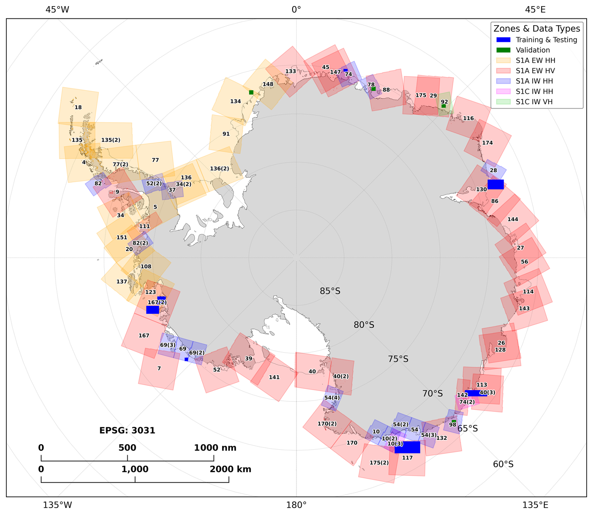
Figure 1 Spatial distribution and coverage of the Sentinel-1 SAR imagery dataset used in this study. The map illustrates the geographic footprints of individual SAR granules along the Antarctic coastline. Footprint colours distinguish between different sensor platforms, swath modes, and polarisations. The opaque rectangular regions define the spatial domains selected for the machine learning workflow, with blue areas representing the training and testing zones, and the green areas representing the independent validation zones. Numeric labels correspond to the ESA-defined relative orbits.

In addition to Sentinel-1 SAR data, this study incorporated multiple supplementary datasets to support iceberg detection and validation. Topographic information was derived from the International Bathymetric Chart of the Southern Ocean (IBCSO; Dorschel et al., 2022) Version 2. Daily sea ice concentration (SIC) data were obtained from the European Organisation for the Exploitation of Meteorological Satellites Ocean and Sea Ice Satellite Application Facility (OSI SAF) Global Sea Ice Concentration product (OSI-408-a), derived from the Advanced Microwave Scanning Radiometer 2 (AMSR2) with a grid resolution of 10 km (EUMETSAT Ocean and Sea Ice Satellite Application Facility (OSI SAF), 2025). Coastline boundaries were referenced from the high-resolution vector data of the Antarctic Digital Database (ADD, Version 7.11; Gerrish et al., 2025) maintained by the Scientific Committee on Antarctic Research (SCAR). Furthermore, optical imagery from the Sentinel-2 MultiSpectral Instrument (MSI; European Space Agency, 2015) was acquired to assist with manual annotation, ground-truth generation, and accuracy assessment. All supplementary datasets provided complete circum-Antarctic coverage, with the temporal window focused on late February to early April 2025, corresponding to the annual minimum of the Antarctic fast ice extent (Fraser et al., 2021), in the year of the lowest summertime fast ice extent on record (Abram et al., 2025).

3 Methods

This section outlines the novel approach for producing the grounded iceberg dataset, and is structured into five main sections: (3.1) data preparation, (3.2) iceberg detection, (3.3) grounded iceberg identification, (3.4) physical constraint filtering, and (3.5) performance validation. The workflow is illustrated in Fig. 2. Boxes I through IV constitute the core production pipeline, progressing from data input to the generation of the final grounded iceberg dataset, while Box V details the accuracy assessment conducted on an independent validation set.

Figure 2 Technical workflow of the grounded iceberg detection and identification system. The pipeline processes Sentinel-1 imagery through deep learning segmentation, individual identification, and physical constraint filtering to generate the final circum-Antarctic grounded iceberg dataset.

3.1 Data preparation and training dataset construction

3.1.1 Generation of training samples

For training U-Net-based models, iceberg regions were manually annotated to create the training dataset. The images were then divided into sub-images of approximately 250×250 pixels each. The exact tile dimensions were dynamically adjusted to ensure integer divisibility, thereby eliminating residual edge strips. Finally, sub-images were upsampled to 1536×1536 pixels using bilinear interpolation, as empirical tests indicated this resolution enhances boundary segmentation accuracy. From a total of 15 SAR images (yielding 4220 sub-images), 702 sub-images containing icebergs under various environmental conditions were manually selected. The iceberg regions were then manually annotated using the Python LabelMe library. The accuracy of the manually drawn masks has been reported to be within 2 %–4 % of the iceberg area (Braakmann-Folgmann et al., 2022), and were verified by at least one study co-author. We generated binary mask images of the same size as the original images from the annotation files, defining pixels within the annotated regions as iceberg and all other pixels as background, as shown in Fig. 3.

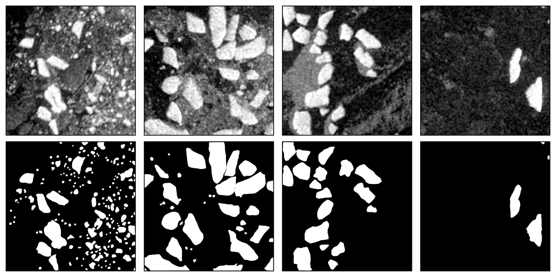
Figure 3 Cropped examples (10×10 km) from input SAR images acquired in Sentinel-1 EW mode with HV polarisation (top row) and corresponding binary masks generated from manual annotations (bottom row).

3.1.2 Model training dataset

For the model training dataset, nine coastal regions of Antarctica were selected to cover a diverse range of environmental conditions (Fig. 1). The data were processed using the method described in Sect. 3.1.1 to construct the training dataset for iceberg detection. This training dataset covers data from February to March in 2021, 2023, and 2025, comprising a diverse mix of imagery from IW and EW swath modes, and spanning both HV and HH polarisations. These specific years were selected to capture a broad range of inter-annual variability in sea ice conditions and iceberg concentrations over a five-year period, ensuring the model's robustness across different environmental regimes. In terms of target selection, the dataset primarily focuses on icebergs smaller than 100 km² (micro to medium-sized), maximising sensitivity for these challenging, under-represented targets. To enable robust generalisation across these differing signal characteristics, a single ResUNet model was trained on this diverse dataset. This strategy allows the network to learn feature representations applicable to both polarisations, thereby mitigating the detection challenges associated with the lower contrast between icebergs and sea ice inherent in HH data. The final dataset was manually divided into a training set for model learning (618 sub-images, 88 %) and a test set (84 sub-images, 12 %) for assessing training performance. This internal assessment is distinct from the final performance validation, which is conducted on an independent validation dataset.

3.1.3 SAR Imagery for grounded iceberg dataset

To construct the circum-Antarctic grounded iceberg dataset, we acquired Sentinel-1 SAR imagery of the entire Antarctic continental shelf coastal margin primarily from March 2025, with the temporal window extended to late February and early April to ensure complete spatial coverage (Fig. 1). This observation period was chosen to coincide with the timing of annual minimum of Antarctic fast ice extent (Fraser et al., 2021). Crucially, the record low fast ice extent observed in early 2025 minimises the risk of misidentifying temporarily immobilised floating icebergs as grounded (Abram et al., 2025). For each orbital track, repeat-pass images with temporal baselines of 12 d (or multiples due to data availability) were analysed. All Antarctic coastal regions included in the dataset are covered by at least two consecutive valid SAR acquisitions, ensuring that no regions were excluded from the stationarity evaluation due to a lack of repeat-pass data. Because our tracking framework analyses these repeat-pass images along the same track, the image pairs used for cross-temporal matching consist of the same acquisition mode and polarisation. Furthermore, continuous image sequences (n≥2) are routinely utilised to assess target stationarity. The dataset comprises a total of 274 Sentinel-1 SAR images, of which 197 were acquired in EW mode and 77 in IW mode. The total cumulative area of the acquired imagery is 9 983 860 km², corresponding to a unique footprint (union area) of 7 456 633 km² and an overlapping area of 2 527 226 km².

3.2 Iceberg detection

This study employs a modified U-Net model (Ronneberger et al., 2015), in which the encoder is replaced by a ResNet152 network (He et al., 2016), forming a ResUNet architecture (Diakogiannis et al., 2020) to enhance the extraction of iceberg features from SAR images. The model takes 1536×1536 single-channel backscatter sub-images as input (as described in Sect. 3.1.1 and shown in Fig. 3), with corresponding manually-annotated masks of the same size indicating iceberg regions and background for training.

3.2.1 Model architecture

To enhance the model's ability to extract features from complex Antarctic coastal environmental backgrounds, this study employs ResNet152 (He et al., 2016) as the encoder and incorporates the Convolutional Block Attention Module (CBAM; Woo et al., 2018) to strengthen attention in both the channel dimension (identifying which features are meaningful) and the spatial dimension (localising where target objects are). The model consists of an encoder, decoder, skip connections, and embedded CBAM (Fig. 4). The encoder uses an ImageNet-pretrained (Deng et al., 2009) ResNet152 to extract multi-scale iceberg features. To accommodate single-channel input, the first convolutional layer is modified to accept single-channel data, and the first four convolutional blocks (convolution, batch normalisation, Rectified Linear Unit (ReLU), and max pooling) are frozen to preserve low-level feature stability, thereby enhancing the model’s robustness in capturing iceberg edges and textures. CBAMs are placed at five levels within the encoder to filter the features. By enhancing the contrast between important targets and the environment, these modules help the model highlight icebergs while ignoring confusing background details like sea ice. The decoder progressively restores spatial resolution through upsampling (nearest-neighbour interpolation) and convolutional operations, fusing features with the corresponding encoder levels. Finally, a 1×1 convolution maps the multi-channel feature representations onto a single-channel probability map, representing the likelihood of each pixel belonging to either iceberg or background, and a probability threshold of 0.5 is applied to binarise the map and generate the iceberg mask.

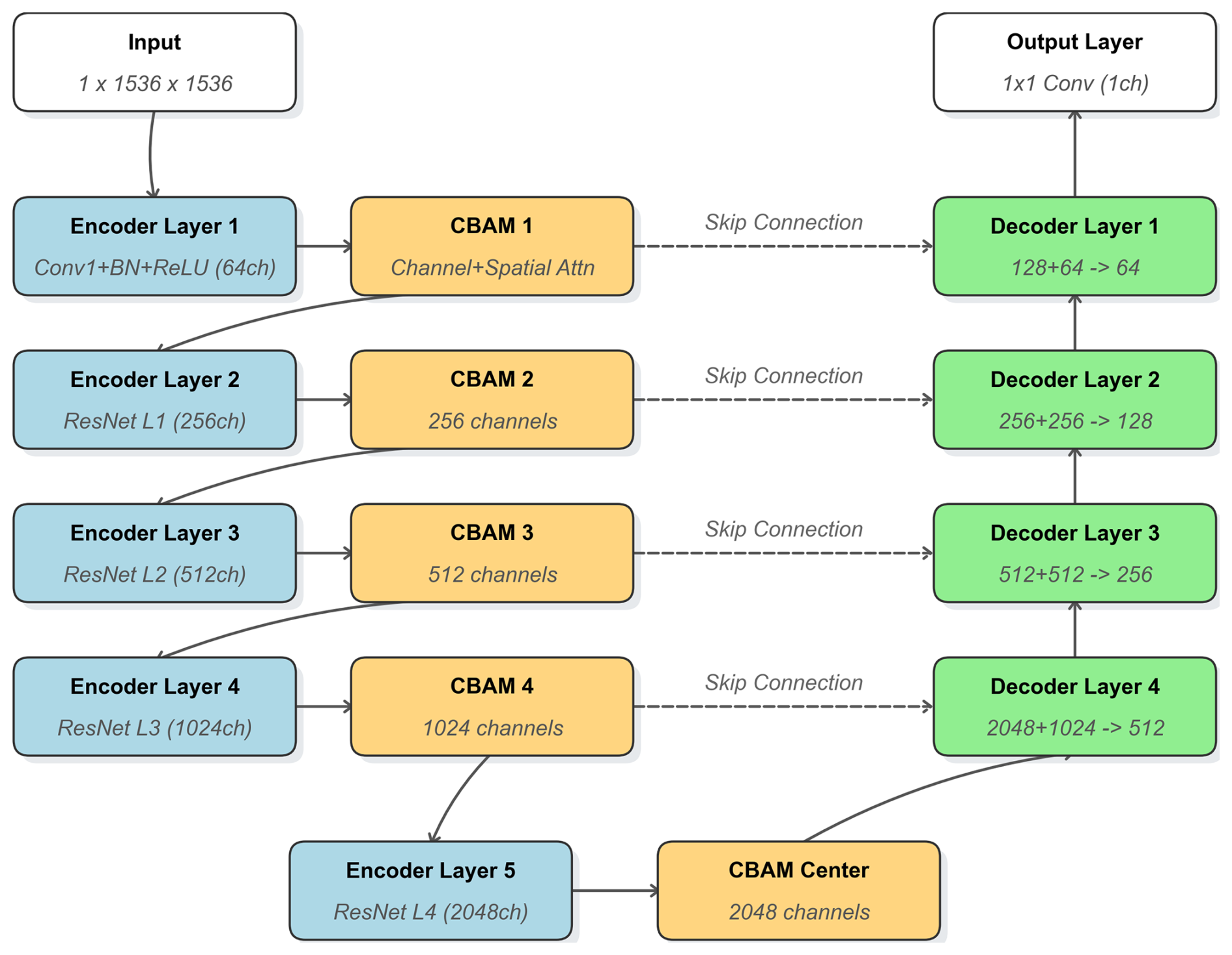
Figure 4 Schematic diagram of the proposed CBAM-ResUNet architecture.The network follows a standard encoder-decoder structure with a ResNet-152 backbone. The encoder path (left, blue nodes) extracts hierarchical features from the single-channel input. To enhance feature representation, Convolutional Block Attention Modules (CBAM, orange nodes) are integrated at the bottleneck and skip connections (dashed lines), applying both channel and spatial attention mechanisms to refine feature maps before fusion. The decoder path (right, green nodes) progressively recovers spatial resolution through upsampling and convolution operations to generate the final binary output mask. Acronyms: ResNet (Residual Neural Network); CBAM (Convolutional Block Attention Module); BN (Batch Normalization); ReLU (Rectified Linear Unit); Conv (Convolution); 1ch (1 Channel).

3.2.2 Model training and optimisation

To determine the optimal training parameters, Bayesian optimisation (Snoek et al., 2012) was employed to search hyperparameters, including learning rate, batch size, and weight decay. The selected training parameters were as follows: learning rate of $\mathrm{3}\times {\mathrm{10}}^{-\mathrm{4}}$, batch size of 4, and weight decay coefficient of $\mathrm{1}\times {\mathrm{10}}^{-\mathrm{4}}$, balancing model convergence speed and segmentation accuracy. In total, approximately 50 independent training runs were executed during the tuning phase and final training runs using the selected optimal configuration.

Iceberg pixels occupy only a small proportion of each image, and the distribution of positive and negative regions is highly imbalanced. To address this, the study employed a combined loss function (L_Total), which linearly integrates weighted Binary Cross-Entropy (L_BCE) and Tversky loss (L_Tversky) (Salehi et al., 2017). The weighted BCE loss is defined as:

$$\begin{array}{}\text{(1)}& L_{\text{BCE}}=-{\displaystyle \frac{\mathrm{1}}{N}}\sum _{i=\mathrm{1}}^N\left[w\cdot y_i\cdot \log \left(\mathit{\sigma }\left(x_i\right)\right)+\left(\mathrm{1}-y_i\right)\cdot \log \left(\mathrm{1}-\mathit{\sigma }\left(x_i\right)\right)\right],\end{array}$$

where N is the total number of pixels, y_i is the ground truth pixel value (0 for background, 1 for iceberg), σ(x_i) is the sigmoid activation of the model output logits x_i, and w represents the positive sample weight. To further mitigate the impact of class imbalance and reduce false negatives, the Tversky loss is calculated based on the Tversky Index:

$$\begin{array}{}\text{(2)}& {\displaystyle }\text{Tversky Index}={\displaystyle \frac{\text{TP}+\mathit{ϵ}}{\text{TP}+\mathit{\alpha }\cdot \text{FP}+\mathit{\beta }\cdot \text{FN}+\mathit{ϵ}}},\text{(3)}& {\displaystyle }{L}_{\text{Tversky}}=\mathrm{1}-\text{Tversky Index},\end{array}$$

where TP, FP, and FN represent pixel-level true positive, false positive, and false negative counts, respectively. The parameters α=0.6 and β=0.4 are set to impose a heavier penalty on false positives compared to false negatives, while ϵ is a small constant (set to $\mathrm{1}\times {\mathrm{10}}^{-\mathrm{6}}$) added to ensure numerical stability and avoid division by zero. The final combined loss function is expressed as:

$$\begin{array}{}\text{(4)}& L_{\text{Total}}=\mathrm{0.4}\cdot L_{\text{BCE}}+\mathrm{0.6}\cdot L_{\text{Tversky}},\end{array}$$

where the weights 0.4 and 0.6 balance the contributions of each loss component to maintain segmentation accuracy while effectively reducing target omission.

Model training was conducted in a multi-GPU parallel environment using the Distributed Data Parallel (DDP) framework to improve training efficiency, with a gradient accumulation step of 2 to achieve a larger effective batch size. The AdamW optimiser (Loshchilov and Hutter, 2017) was used in combination with a cosine annealing learning rate scheduler, completing a full cycle every 20 epochs, with a minimum learning rate of $\mathrm{1}\times {\mathrm{10}}^{-\mathrm{6}}$. To further stabilise training, automatic mixed precision (AMP; Micikevicius et al., 2017) and gradient scaling were applied to optimise computational efficiency. An early stopping mechanism was implemented, terminating training when the F1 score on the test set did not improve for 10 consecutive epochs, and the best-performing model was saved. In practice, each model typically required approximately 20–30 epochs to reach convergence.

In terms of computing resources, training was conducted on four NVIDIA Tesla V100 32GB GPUs within the Australian National Computational Infrastructure (NCI) Gadi supercomputer. Each training session took approximately half an hour.

3.3 Grounded iceberg identification

In this study, stationary icebergs are detected through a hierarchical filtering framework that integrates spatiotemporal identification with environmental constraints. We initially define a stationary iceberg candidate as a feature that persists at a fixed location for a minimum duration of 12 d. However, stationarity alone does not imply grounding, as icebergs may also be immobilised by fast ice. To operationalise this definition, we developed a multi-stage grounded iceberg identification pipeline, comprising three key phases: (1) individual iceberg extraction (Sect. 3.3.1), which isolates distinct iceberg entities from segmentation masks; (2) stationary target identification (Sect. 3.3.2), which establishes temporal continuity based on geometric similarity and motion constraints defined by a maximum centroid displacement of 10 pixels; and (3) quality control, which mitigates false positives using bathymetric, surrounding sea ice concentration criteria. Only candidates that survive this rigorous screening process are classified as stationary icebergs. We then use a March 2025 map of fast ice extent (Abram et al., 2025) to suggest which stationary icebergs are “high-confidence grounded” vs those possibly rendered stationary due to enclosure by fast ice.

3.3.1 Individual iceberg extraction

Since the binary masks predicted by the U-Net model provide only pixel-level classification without differentiating between individual iceberg instances, they cannot inherently distinguish individual icebergs. To address this, we implemented a block-based parallel processing method for connected component extraction. Given the wide coverage of SAR EW and IW modes and the density of small icebergs, masks are partitioned into multiple blocks to optimise processing. Each block undergoes independent connected component analysis using OpenCV (Bradski, 2000) to generate local labels and compute geometric properties (e.g., area, centroids, and bounding box), while regions smaller than 10 pixels are discarded as noise. Among these properties, the axis ratio is estimated through ellipse fitting to describe each iceberg's elongation:

$$\begin{array}{}\text{(5)}& \text{Axis Ratio}={\displaystyle \frac{a}{b}},\end{array}$$

where a and b are the lengths of the major and minor axes, respectively. To mitigate pixel-level quantisation errors and improve the reliability of subsequent shape-based matching, the extracted contours are smoothed using a moving average convolution:

$$\begin{array}{}\text{(6)}& p_i^{\prime }=\sum _{j=-k}^k{p}_{i+j}\cdot {\displaystyle \frac{\mathrm{1}}{\mathrm{2}k+\mathrm{1}}},\end{array}$$

where p_i is the original coordinate (x_i or y_i) of the i-th contour point, $p_i^{\prime }$ is the resulting smoothed coordinate, and k is half of the kernel size used for the smoothing convolution. Simultaneously, to eliminate false positives arising from glacier features, we incorporated the SCAR ADD high-resolution Antarctic coastline polygons (Gerrish et al., 2025); any candidate region overlapping with these land masks is automatically excluded.

To resolve the splitting of connected regions across block boundaries, a Union-Find algorithm (Galler and Fisher, 1964) is applied to merge boundary labels. Subsequently, each connected region is mapped to a global label with a unique identifier, ensuring consistent representation across blocks. Ultimately, the workflow generates single-channel label masks for each individual iceberg, accompanied by a detailed attribute dataset (including area, centroid, and ID), providing the necessary data foundation for grounded iceberg identification and analysis.

3.3.2 Grounded iceberg identification algorithm

In this study we develop an algorithm for identifying grounded icebergs in SAR imagery, aimed at monitoring grounded icebergs using the multi-temporal mask data and region information obtained in Sect. 3.3.1. The method integrates block-based processing, feature extraction, cost matrix optimisation, and trajectory management, making it suitable for large-scale analysis of grounded icebergs in SAR data. The algorithm is structured into three main components: (1) data input, (2) processing workflow, and (3) output results.

In the data input stage, the algorithm primarily takes iceberg region information files and the corresponding single-channel mask files as inputs. The process begins with region loading and tile-based partitioning. Imagery and geographic information data, including the coordinate reference system and affine transformation matrix, are read using the Rasterio Python library (Gillies, Sean and others, 2013), and the images are divided into tiles. Each region is then assigned to the corresponding tile based on its centroid location. The algorithm then extracts multiple features for each region, including the binary region and its properties from the mask (Sect. 3.3.1), contours and smoothed contours derived using OpenCV, and the major-to-minor axis ratio through ellipse fitting, providing a comprehensive description of each iceberg’s shape and characteristics.

The grounded iceberg spatiotemporal association component achieves trajectory continuation through cross-temporal region matching. The method employs the Hungarian algorithm (Kuhn, 1955) for cost matrix optimisation. The assignment problem is formulated to find the optimal matching that minimises the total cost:

$$\begin{array}{}\text{(7)}& min\sum _{i,j}{C}_{ij}\cdot x_{ij}\end{array}$$

subject to:

$$\begin{array}{}\text{(8)}& \sum _j{x}_{ij}=\mathrm{1},\sum _i{x}_{ij}=\mathrm{1},x_{ij}\in \mathit{\{}\mathrm{0},\mathrm{1}\mathit{\}},\end{array}$$

where C_ij is the element of the cost matrix representing the matching cost between region i and trajectory j, and x_ij is a binary variable indicating whether region i is assigned to trajectory j. For regions within the same tile across consecutive temporal phases, the cost matrix C_ij was constructed incorporating multiple metrics:

$$\begin{array}{}\text{(9)}& \begin{array}{rl}{C}_{ij}& =w_{\mathrm{1}}\cdot \text{norm\_dist}(c_i,c_j)\\ & +w_{\mathrm{2}}\cdot \text{norm\_area}(M_i,M_j)\\ & +w_{\mathrm{3}}\cdot \text{norm\_axis}(R_i,R_j,{\mathit{\theta }}_i,{\mathit{\theta }}_j)\\ & +w_{\mathrm{4}}\cdot \text{norm\_contour}(S_i,S_j),\end{array}\end{array}$$

where $w_{\mathrm{1}},w_{\mathrm{2}},w_{\mathrm{3}},w_{\mathrm{4}}$ are weights assigned to each metric ($w_{\mathrm{1}}=\mathrm{0.05},w_{\mathrm{2}}=\mathrm{0.30},w_{\mathrm{3}}=\mathrm{0.60},w_{\mathrm{4}}=\mathrm{0.05}$). The components include the normalised centroid Euclidean distance, region-overlap cost, axis ratio, and contour-shape similarity based on Hu invariant moments (Hu, 1962). The region-overlap cost is calculated using the Intersection over Union (IoU):

$$\begin{array}{}\text{(10)}& \text{IoU}(M_{\mathrm{1}},M_{\mathrm{2}})={\displaystyle \frac{|M_{\mathrm{1}}\cap M_{\mathrm{2}}|}{|M_{\mathrm{1}}\cup M_{\mathrm{2}}|}},\end{array}$$

where M₁ and M₂ are the binary mask regions at two consecutive timestamps, $|M_{\mathrm{1}}\cap M_{\mathrm{2}}|$ is the number of overlapping pixels, and $|M_{\mathrm{1}}\cup M_{\mathrm{2}}|$ is the number of pixels in the union. Hu moments, being invariant to translation, rotation, and scaling, enhance the robustness of the matching algorithm by quantifying shape similarity through the logarithmic differences of seven invariant moments.

To improve matching accuracy, the algorithm first excludes region pairs with excessive spatial separation using a centroid distance threshold (10 pixels), followed by filtering based on area difference (threshold 0.5) and IoU threshold (0.99, i.e., IoU <0.01) to eliminate anomalous matches. If the total cost is below the threshold of 10⁶ and represented the optimal solution within the matchable range, the regions are deemed to correspond to the same iceberg across different times, and the trajectory information is updated; if no match is found, a new trajectory is initiated. If a grounded iceberg is missed in a single timestamp due to detection errors or merging with nearby icebergs but reappears in subsequent frames, the algorithm automatically reconnects its trajectory.

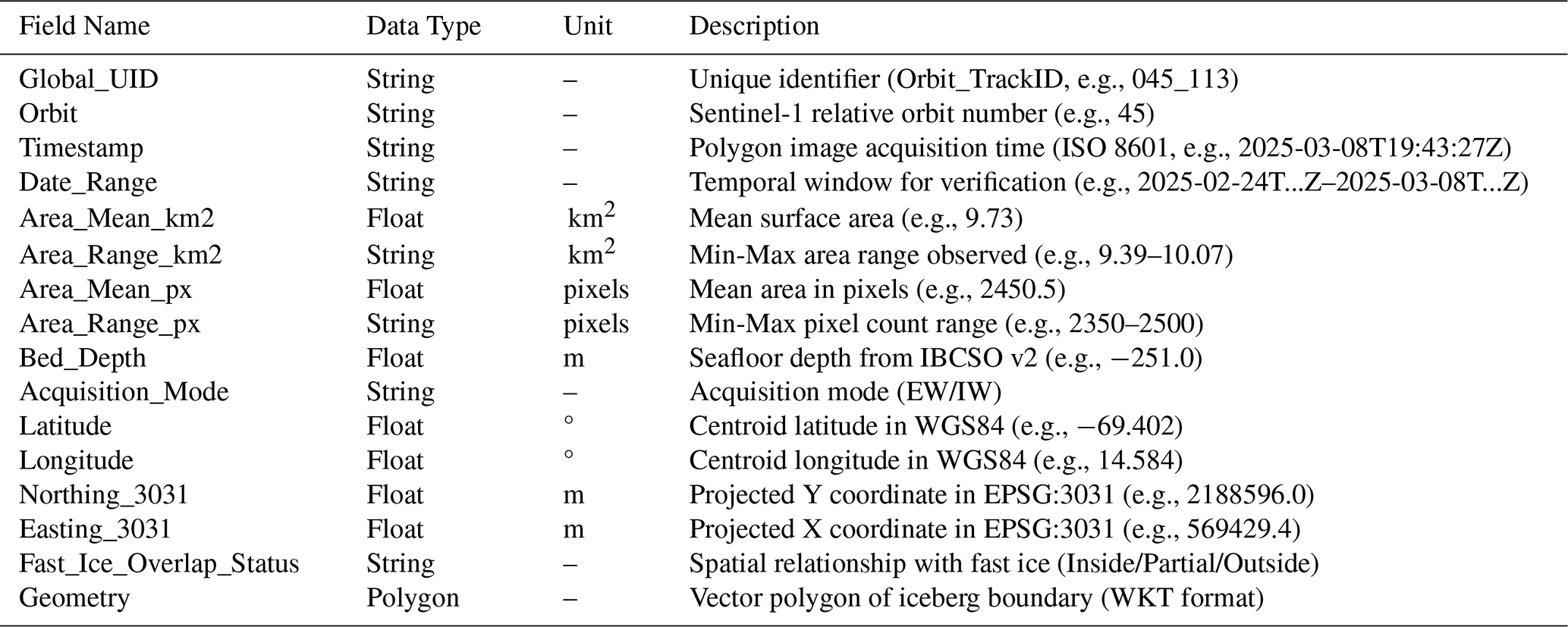
The identification results are exported as a tabular data file, with each trajectory record containing information such as timestamp, centroid, area, unique identifier, and matching cost. This data file, combined with multi-temporal mask data, forms the grounded iceberg dataset, the structure of which is detailed in Table 1.

Table 1 Structure and description of the circum-Antarctic grounded iceberg dataset attributes. UID stands for Unique ID, EW stands for Extra Wide swath mode, IW stands for Interferometric Wide swath mode, and WKT stands for Well-Known Text.

3.4 Physical constraint filtering

Although the stationarity-based identification algorithm (Sect. 3.3.2) effectively distinguishes stationary from drifting targets, two main types of false positives can still occur in regions of high ice concentration or deep water: (1) floating icebergs temporarily immobilised by surrounding sea ice (especially fast ice, which can arrest iceberg advection; e.g., as shown in Fig. 6 of Fraser et al., 2010), and (2) strong backscatter signals from dense sea ice rubble or ice deformation. To ensure the physical plausibility of the grounded iceberg dataset, we applied post-processing filters incorporating bathymetry and SIC data.

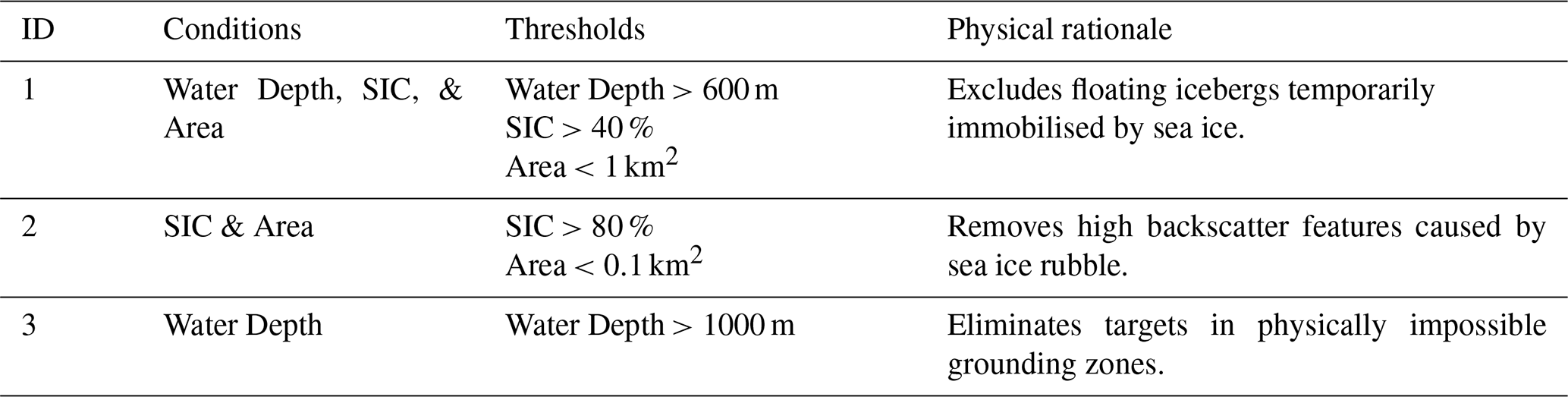
Identified iceberg trajectories were spatially matched with IBCSO bathymetry (Dorschel et al., 2022) and spatiotemporally aligned with daily AMSR2 SIC data (EUMETSAT Ocean and Sea Ice Satellite Application Facility (OSI SAF), 2025). Based on Antarctic grounded iceberg characteristics (Massom et al., 2001; Dowdeswell and Bamber, 2007, as noted in Sect. 1), three hierarchical filtering criteria were defined (Table 2). Trajectories meeting any exclusion criterion at any time step were flagged as invalid and removed from the final dataset. This procedure markedly reduced false positives under complex sea ice conditions, ensuring high geographical and physical confidence in the resulting dataset. The quantitative impact of each filtering stage on the final grounded iceberg dataset is detailed in Sect. 4.2.1.

Table 2 Parameters for post-processing quality control filters. SIC: Sea Ice Concentration.

Preliminary visual inspection indicated that the dataset from orbit 54 (∼146° E) exhibited anomalous textural characteristics, likely attributable to complex sea ice conditions. The presence of heavily deformed sea ice and surface roughness resulted in high backscatter signals that resembled the signature of icebergs. This environmental complexity led to widespread false positives, manifesting as small, fragmented artefacts. Furthermore, this region was not used in training the deep learning model. To mitigate this spatial heterogeneity, we implemented an ad-hoc quality control filtering strategy, applying a more stringent area threshold exclusively to this orbit: all tracked icebergs containing any individual observation smaller than 200 pixels (approximately 0.08 km²) were discarded. This targeted intervention effectively suppressed persistent noise artefacts in this orbit, and ensured that the reliability of the extracted trajectories in this region was consistent with that of the remainder of the global dataset.

To distinguish between truly grounded icebergs and floating icebergs immobilised by landfast sea ice, we performed a spatial overlay analysis using a high-resolution fast ice mask digitised from the same time period as the SAR data used in this study (Abram et al., 2025). Fast ice digitisation was manually achieved using a high-resolution cloud-free visible image composite, as described by Fraser et al. (2009). Each stationary iceberg candidate was then classified based on its spatial relationship with this mask:

1. Inside: The stationary iceberg geometry is completely contained within the fast ice boundary, indicating that it may not be grounded.

2. Partial: The stationary iceberg geometry intersects the fast ice boundary but is not fully contained. This often occurs on the “downstream” side (typically to the west) of persistent fast ice features, and often indicates genuinely grounded icebergs which support fast ice growth and stability on the “upstream” side (typically to the east) (Fraser et al., 2012).

3. Outside: The stationary iceberg has no spatial overlap with the fast ice mask. Targets classified as “Outside” are identified as high-confidence grounded icebergs, as no fast ice is present to inhibit their motion.

3.5 Validation

3.5.1 Iceberg detection model performance

To evaluate the performance of the iceberg detection model, we conducted an independent validation of the ResUNet model using a 50×50 km region in Adélie Land (∼136° E) as the validation dataset. We manually interpreted and annotated 12 images, acquired in EW swath mode with cross-polarisation (HV) at monthly intervals from January 2021 to December 2021, thereby establishing the ground-truth dataset for the icebergs. We chose to perform a year-round validation, even though the training dataset is only selected from the months of February and March. This allows us to assess the generalisation of our proposed method across different seasons and possible limitations caused by surface melt during the summer. The validation set underwent no data augmentation and was not used during model training, ensuring that the evaluation objectively reflects the model's performance and generalisation ability. To ensure the reliability of these manual annotations, Sentinel-2 MSI optical imagery was utilised as an auxiliary reference for visual verification (e.g., to allow manual separation of small icebergs from similarly-shaped small sea ice floes).

To ensure the model's robustness and representativeness at the circum-Antarctic scale, we constructed an extended validation dataset comprising three additional independent observational scenes acquired between late February and mid-April 2025. These scenes were purposefully selected to cover all combinations of Sentinel-1 acquisition modes (EW and IW) and available polarisations (HH and VH) used in this study, enabling an assessment of how differing radar configurations affect single-frame detection performance.

During validation, we computed standard pixel-wise performance metrics, including producer’s accuracy (recall), user’s accuracy (precision), and F1 score (the harmonic mean of precision and recall). Based on the comparison between the predicted and ground-truth masks, true positives (TP), true negatives (TN), false positives (FP), and false negatives (FN) were recorded. These confusion categories are defined as follows: TP represents pixels correctly predicted as iceberg; TN represents pixels correctly predicted as background; FP represents pixels incorrectly predicted as iceberg; and FN represents pixels incorrectly predicted as background. These counts were then used to calculate the core performance metrics:

$$\begin{array}{}\text{(11)}& {\displaystyle }\text{Precision}={\displaystyle \frac{\text{TP}}{\text{TP}+\text{FP}+\mathit{ϵ}}},\text{(12)}& {\displaystyle }\text{Recall}={\displaystyle \frac{\text{TP}}{\text{TP}+\text{FN}+\mathit{ϵ}}},\text{(13)}& {\displaystyle }\text{F1}={\displaystyle \frac{\mathrm{2}\cdot \text{Precision}\cdot \text{Recall}}{\text{Precision}+\text{Recall}+\mathit{ϵ}}},\text{and}\text{(14)}& {\displaystyle }\text{FAR}={\displaystyle \frac{\text{FP}}{\text{FP}+\text{TN}+\mathit{ϵ}}},\end{array}$$

where ϵ is a small constant (set to $\mathrm{1}\times {\mathrm{10}}^{-\mathrm{6}}$) added to ensure numerical stability and avoid division by zero. Precision measures the proportion of predicted “iceberg pixels’” that are truly icebergs, reflecting the reliability of the model’s predictions; recall measures the proportion of all actual iceberg pixels that are successfully detected by the model, indicating its tendency to miss targets; and False Alarm Rate (FAR) measures the proportion of background pixels incorrectly classified as iceberg pixels, reflecting the model’s false detection rate.

3.5.2 Grounded iceberg identification

We also used the same 50×50 km area in Adélie Land, as described in Sect. 3.5.1, as the validation scene for the grounded iceberg identification algorithm. The evaluation employed a frame-based statistical approach, in which the identification results were manually classified. The specific evaluation metrics are defined as follows:

1. TP: the number of frames in which the algorithm successfully identified the grounded iceberg. That is, at a given time, the algorithm assigns the iceberg to the correct trajectory.

2. FN: the number of frames in which a grounded iceberg is actually present but the algorithm fails to generate a valid tracking result, also referred to as `missing frames’. This reflects instances where the algorithm loses the target in the time series.

3. FP: the number of frames in which the algorithm incorrectly generates a tracking result. This includes cases where background elements (such as sea ice or waves) are misidentified as grounded icebergs, or incorrectly classifies icebergs from different times as belonging to the same grounded iceberg.

Based on the above statistics, we selected Precision, Recall and F1 Score as the core evaluation metrics.

4 Results

Following the classification scheme of Wesche and Dierking (2015), the detected icebergs were divided into six categories based on their area: micro icebergs (A0, <0.1 km²), tiny icebergs (A1, 0.1–1 km²), small icebergs (A2, 1–10 km²), medium icebergs (A3, 10–100 km²), large icebergs (A4, 100–1000 km²), and giant icebergs (A5, ≥1000 km²). This classification enables effective differentiation of spatial distribution patterns across icebergs of varying sizes. However, it is important to note that no grounded icebergs belonging to the large (A4) or giant (A5) categories were identified in this dataset. This aligns with our research focus on resolving the “missing” population of smaller icebergs (<100 km²), complementing the comprehensive records of large targets maintained by operational agencies (e.g., U.S. National Ice Center; U.S. National Ice Center, 2024). Consequently, our training strategy prioritised micro to medium icebergs (A0–A3) to ensure maximum sensitivity for these challenging, under-represented targets.

4.1 System performance evaluation

Using the independent validation set from Adélie Land described in Sect. 3.5, we conducted a systematic evaluation of the ResUNet model and the iceberg identification algorithm. The complex environmental characteristics of this region, which present substantial background clutter and variability, provide a suitable setting for assessing the robustness of the model in pixel-level detection and temporal tracking.

4.1.1 Iceberg detection performance

In terms of iceberg detection, the ResUNet model demonstrated strong and reliable performance on both the validation and test datasets. The model stopped training on the manually-partitioned test set with an F1 score of 0.8926, a precision of 0.8963, a recall of 0.9002, and a FAR of 0.0058. Its performance on the 50×50 km validation region in Adélie Land was similarly strong, achieving an average precision of 0.9145, a recall of 0.9131, an F1 score of 0.9121, and a false alarm rate of 0.0056 across twelve months. Table 3 presents the model’s performance metrics across selected images from different months.

Table 3 Monthly test metrics for the iceberg detection model. FPR: false positive rate.

These metrics indicate that the model is capable of accurately and consistently detecting iceberg pixels, while maintaining a low rate of background pixels erroneously classified as icebergs. The statistical results presented in Table 3 further confirm the model’s cross-seasonal generalisation. With the exception of December the model maintained a high level of detection stability throughout most of the year. The reduced model performance in December is likely caused by changes in backscatter resulting from surface melt and moisture in the snow cover, which is confirmed by visual inspection of example images from multiple regions. However, recall that December is not used for the generation of the final grounded iceberg dataset presented here. Except for these seasonal effects, the model handles changes in sea ice coverage and complex sea states effectively, demonstrating strong robustness in Antarctica’s dynamic coastal environment. Figure 5 illustrates representative test samples, including the raw SAR imagery, Sentinel-2 optical imagery, manually annotated ground truth, and the model’s predicted masks. Visual inspection shows a high degree of agreement between the predicted iceberg boundaries and the ground truth. Notably, for icebergs with irregular edge morphology, the model produces smooth and well-fitted contours, demonstrating its effectiveness in preserving geometric detail.

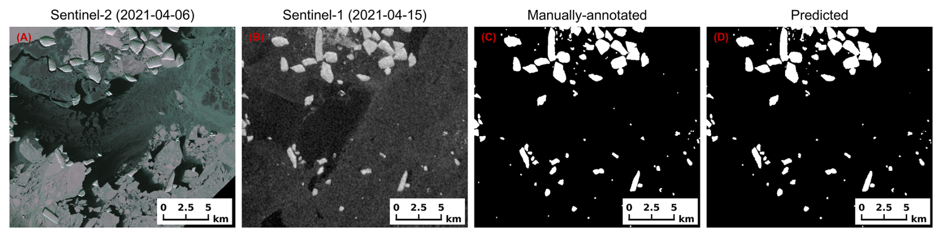
Figure 5 Visual comparison of the iceberg ground truth mask and the predicted mask on SAR imagery (∼136° E). (A) Sentinel-2 optical image acquired on 6 April 2021, shown as a false-colour composite using bands B08 (near-infrared), B04 (red), and B03 (green); (B) Sentinel-1 HV intensity image acquired on 15 April 2021; (C) iceberg ground truth mask obtained through manual annotation based on panel (B); (D) predicted mask generated by the deep learning model from the same Sentinel-1 image. In mask images (C) and (D), white regions represent the identified iceberg bodies, and black regions represent the background ocean or sea ice. Panels (B), (C), and (D) have exactly the same acquisition time (15 April 2021) and geographical extent, while panel (A) serves as a contemporaneous visible reference for validation.

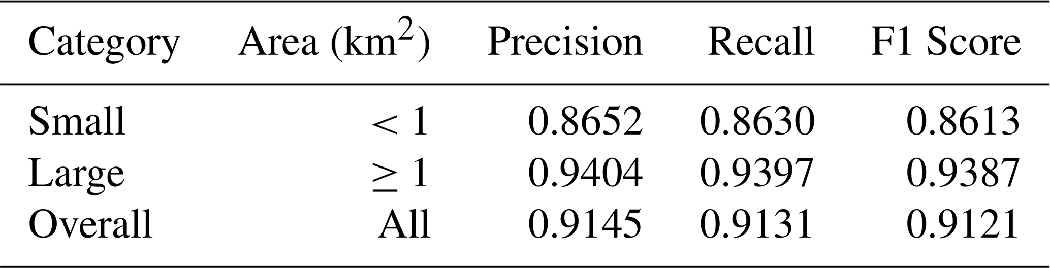
Given the numerical dominance of tiny icebergs(<1 km²) in the Antarctic coastal system, we further conducted a size-stratified performance evaluation. Using a threshold of 1 km², we classified the ground truth targets into “small” (<1 km²) and “large” (≥1 km²) categories. As detailed in Table 4, the model exhibits robust detection capabilities across both size classes. For large icebergs, the model achieved a high Recall of 0.9397, demonstrating its effectiveness in capturing the main bodies of extensive ice shelves and tabular icebergs. Crucially, for the challenging small iceberg category, which is often prone to sea clutter interference, the model maintained a Precision of 0.8652 and an F1 score of 0.8613. These results indicate that the model's high overall performance is not solely driven by large objects but reflects a genuine capability to distinguish sub-kilometer icebergs from complex backgrounds.

Table 4 Size-stratified detection performance (small (<1 km²) vs. large (≥1 km²) icebergs).

The extended validation across different combinations of acquisition modes and polarisations (Table 5) further elucidates the model's sensitivity to radar mode and polarisation. While the model exhibits consistently high performance in cross-polarised imagery (e.g., F1 scores of 0.880 and 0.891 for IW mode, VH polarisation), its single-frame pixel-level accuracy fluctuates in co-polarised (HH) imagery. Specifically, the scenes acquired on 2 March 2025 using EW mode with HH polarisation and on 11 March 2025 using IW mode with HH polarisation show substantial drops in Precision (0.4908 and 0.4528, respectively) and overall F1 scores (∼0.61).

Table 5 Extended pixel-level detection performance across different acquisition modes and polarisations.

Confusion matrix analysis reveals that this performance drop stems not from missed targets, as Recall remains robust (e.g., 0.9378 for the 2025-03-11 scene), but from a marked spike in false positive. This is because HH polarisation often yields similar backscatter signatures for icebergs, deformed sea ice, and wind-driven clutter, making single-frame differentiation inherently difficult. Crucially, these single-frame errors do not detract from the final dataset. Most False Positives in HH-polarised images represent transient features, such as drifting floes or transient surface roughness. Being highly mobile, they fail the strict temporal continuity constraints of our tracking algorithm (Sect. 3.3.2). Therefore, while varying polarisations cause unavoidable single-frame segmentation fluctuations, rigorous multi-temporal tracking acts as a robust spatiotemporal filter, neutralising transient noise to ensure a high-confidence final product.

4.1.2 Grounded iceberg identification verification

Building on the validated single-frame iceberg detection performance, we further evaluated the grounded iceberg identification algorithm using the temporal SAR imagery of the Adélie Land validation set. The evaluation employed frame-based statistical metrics, with a focus on the algorithm’s ability to maintain target identity consistency across the temporal sequence.

Quantitative results indicate that the algorithm exhibits high stability over multiple consecutive frames. Frame-level evaluation metrics show a precision of 0.9590, a recall of 0.8660, and an F1 score of 0.9102. The high precision demonstrates that the algorithm effectively avoids misclassifying background noise, such as transient disturbances from drifting sea ice, as new iceberg trajectories. Moreover, few erroneous matches occur within the generated trajectories. The relatively lower recall is primarily attributed to object merging in densely-populated regions. Although the algorithm is generally able to maintain stable tracking, in areas of high iceberg density, adjacent icebergs are prone to being misidentified as a single connected component. Such segmentation errors hinder the generation and maintenance of independent trajectories for individual icebergs, leading to intermittent tracking interruptions or failures.

The robustness of the algorithm is largely attributed to its multi-feature matching strategy based on the Hungarian algorithm. In terms of shape invariance, although icebergs may undergo pixel-level morphological variations due to changes in imaging angle or minor tilting at different observation times, the incorporation of Hu invariant moments (Hu, 1962) plays a critical role. These moments consist of seven statistical descriptors derived from central moments that characterise the global shape distribution and remain theoretically constant under translation, scaling, and rotation. Regarding trajectory continuity, the results presented in Fig. 6 confirm the robustness of the matching algorithm. By jointly utilising mask contours and centroid features, the algorithm achieves reliable object association over the temporal sequence, producing clear and continuous iceberg trajectories and validating the reliability of the matching results. Furthermore, the thresholding mechanism based on IoU and centroid distance effectively removes aberrant drift trajectories of non-grounded icebergs, ensuring that the final grounded iceberg dataset attains a high level of confidence.

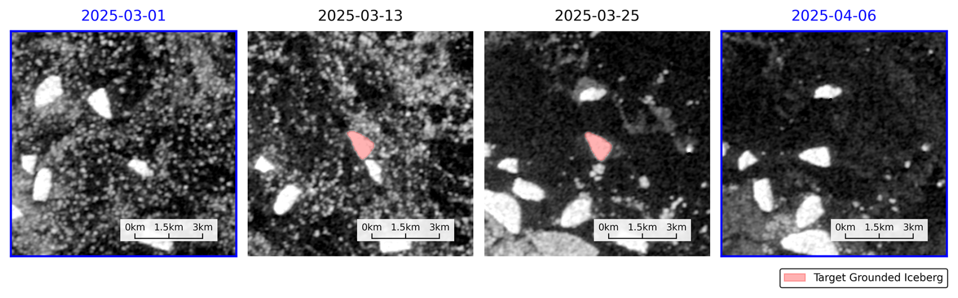
Figure 6 Multi-temporal evolution of an iceberg grounding-ungrounding event. The gallery displays a sequence of Sentinel-1 SAR imagery patches showing the tracked iceberg throughout its grounding event (first two frames), its period of being grounded (middle two frames), and ungrounding (final two frames). The target iceberg is delineated by a red mask during its grounded phase. Images with blue titles indicate reference timestamps confirming that the iceberg was grounded only for the two middle frames.

To quantify the temporal uncertainty of grounded iceberg identification, we evaluated start and end dates of period where the algorithm identified each iceberg as stationary against manual expert assessments for 241 distinct algorithm-derived stationary trajectories (comprising 1452 individual polygons) within the Adélie Land validation set (Table 6). As observed in visual assessments, high-density packing frequently causes adjacent icebergs to be segmented as a single merged polygon, while summer surface meltwater can lead to target fragmentation. Consequently, a single physical iceberg may be represented by multiple trajectories segments, or multiple icebergs by a single trajectory (Fig. S4 in the Supplement).

Table 6 Correct versus incorrect grounded iceberg identification metrics. In this evaluation, temporal sequences of n images are analysed. The terms “Start” and “End” refer to the specific image frame number within the sequence at which an iceberg was first and last identified as stationary by the algorithm. For a detailed explanation of the evaluation methodology, refer to Sect. 4.1.2.

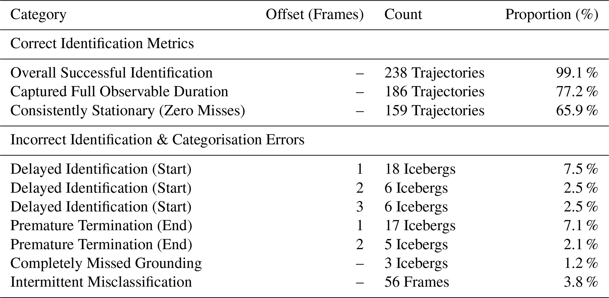
Overall, the algorithm successfully captured the full observable duration of stationarity for the vast majority of these identified trajectories (77.2 %). When evaluating the physical targets corresponding to these trajectories, delayed identification (i.e., cases where the iceberg was assessed manually as stationary prior to the algorithm) occurred in 30 icebergs (12.4 %), lagging by between 1 and 3 frames primarily due to sea-ice clutter obscuring initial target boundaries. Premature terminations (i.e., cases where the manually assigned period of stationarity extended longer than the algorithm's assessment) affected 22 icebergs (9.1 %), ending 1 to 2 frames early as summer surface meltwater degraded radar contrast. Complete identification failures were exceptionally rare, occurring in only 3 instances (1.2 %). While intermittent mid-trajectory misses were recorded (56 frame instances), our multi-temporal matching effectively bridged these gaps to maintain overall state continuity.

In summary, the validation results from Adélie Land demonstrate that the identification algorithm can maintain continuous identification and identity consistency of iceberg targets in complex environments, providing a reliable technical foundation for constructing a high-precision, circum-Antarctic grounded iceberg dataset.

4.2 Circum-Antarctic grounded iceberg dataset

Based on the previously validated detection and tracking framework, we applied our method to Sentinel-1 SAR imagery acquired from late February to early April 2025 around the Antarctic coastline (Fig. 1), thereby constructing the first high-resolution circum-Antarctic grounded iceberg dataset. This dataset records the geographic locations, morphological contours, and geometric attributes of each grounded iceberg, revealing the macroscopic distribution patterns of grounded icebergs along the Antarctic coastline.

4.2.1 General Statistics

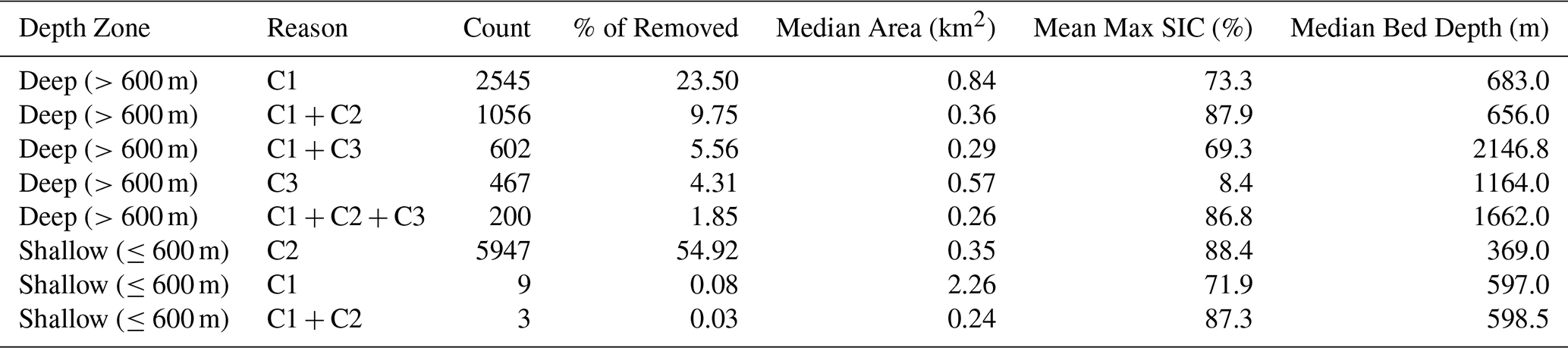
To quantify the effectiveness of the physical constraint filtering (described in Sect. 3.4), we tracked the number of stationary iceberg candidates removed at each stage. From the initial pool of 50 448 tracked stationary targets, 10 829 candidates were eliminated (Table 7).

Table 7 Detailed statistics of iceberg candidates removed by the physical constraint filters. Depth zones are divided into deep (>600 m) and shallow (≤600 m) waters. The “Reason” corresponds to the filter IDs defined in Table 2 (C1: Depth >600 m & SIC >40 % & Area <1 km²; C2: SIC >80 % & Area <0.1 km²; C3: Depth >1000 m). SIC: Sea Ice Concentration.

After filtering, the final dataset consisted of 39 619 stationary targets along the Antarctic continental shelf, with a combined area of 13 430 km². As shown in Fig. 7, the frequency distribution of grounded iceberg areas is strongly skewed towards smaller sizes, with a mean area of 0.34 km² and a median area of 0.13 km². Notably, icebergs with an area of less than 1 km² dominate numerically, accounting for as much as 92.6 % of the total number. By area, tiny icebergs (A0 and A1) also account for 53.90 %. It is important to note that this proportion is likely inflated, as the model's limitation in fully segmenting large and giant icebergs leads to an underestimation of their total area.

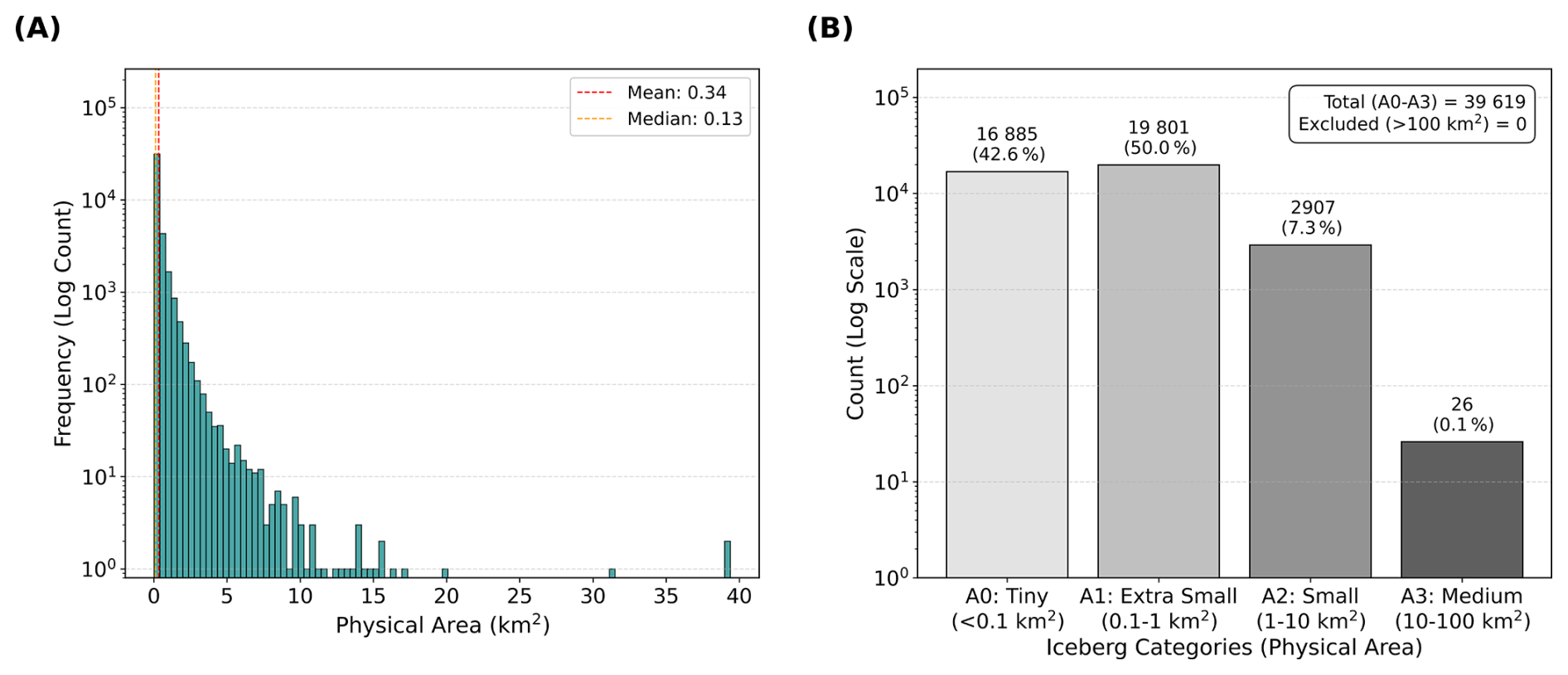
Figure 7 Size distribution analysis of unique grounded icebergs. (A) Frequency distribution of the physical area (km²) for all identified icebergs. The y-axis is presented on a logarithmic scale to account for the high frequency of smaller icebergs. Red and orange dashed lines indicate the mean and median physical areas, respectively. (B) Categorical distribution of icebergs across classes. Labels above the bars indicate the total count and the relative percentage of the total population for each category.

Of the 39 619 stationary targets identified, spatial analysis reveals that 27 634 (67.4 %) are not located within or adjacent to fast ice (i.e., classified as “Outside”), confirming their status as high-confidence grounded. Meanwhile, 11 436 targets are situated completely within fast ice, and 626 exhibit partial overlap. While these “Inside” and “Partial” targets remain stationary, their grounding status is subject to higher uncertainty due to potential fastening by the surrounding fast ice.

4.2.2 Spatial Distribution

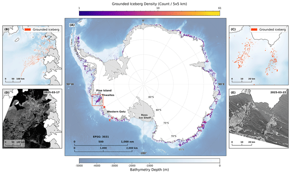
The spatial density of grounded icebergs around Antarctica exhibits heterogeneity. As shown in Fig. 8, nearly all high-density hotspots are concentrated in shallow coastal regions. In these areas, shallow bathymetric features, such as continental banks and ridges, provide favourable anchoring points for iceberg grounding, especially downstream of regions where active ice-shelf calving supplies a plentiful source of icebergs. For example, in regions such as Thwaites Glacier (∼106.75° W) and Fram Bank (∼69.5° E), the maximum density reaches 41 icebergs per 25 km², forming complex coastal “grounded iceberg chains”. In contrast, grounded icebergs are sparsely distributed in deep-water regions, such as Pine Island Trough (∼101° W), where excessive water depths prevent long-term grounding. Similarly, low densities are observed in areas lacking productive upstream sources; notably, while massive ice shelves such as the Ross Ice Shelf (∼180°) produce giant tabular icebergs, they calve infrequently, resulting in fewer individual grounding events compared to smaller, frequently-calving ice shelves.

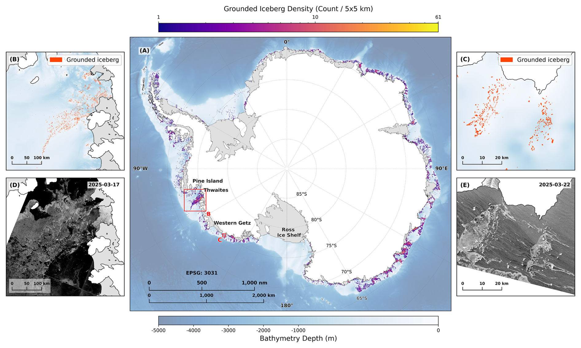
Figure 8 Spatial distribution of grounded icebergs. (A) Circum-Antarctic density heatmap (counts per 5×5 km grid) overlaid on International Bathymetric Chart of the Southern Ocean (IBCSO) bathymetry version 2 (Dorschel et al., 2022). Red boxes indicate the locations of the detail panels. (B, C) Close-up views of Thwaites Glacier and Western Getz Ice Shelf, respectively, displaying individual grounded iceberg polygons (orange) to illustrate their alignment along shallow continental banks. (D, E) Corresponding Sentinel-1 SAR imagery for the regions shown in (B) and (C). Panel (D) shows the Thwaites region (EW mode, HV polarisation) acquired on 17 March 2025, and Panel (E) shows the Western Getz region (IW mode, HH polarisation) acquired on 22 March 2025.

Despite regional heterogeneity, grounded icebergs remain a widely-encountered feature of the Antarctic margin. By projecting iceberg locations onto the main continental coastline and dividing the coast into 100 km intervals, we found that grounded icebergs are present along 56.52 % of the entire coastline, further confirming their role as a widespread boundary condition for the coastal cryosphere. However, their spatial density is highly uneven. Cumulative distribution analysis based on 100 km coastal segments demonstrates extreme spatial clustering in both count and physical area. Specifically, 50 % of the grounded icebergs (by number) are concentrated within only 4.9 % of the coastline, closely mirrored by the distribution of total grounded area (50 % within 3.8 %). Extending to the bulk of the population, 14.2 % of the coastline contains 80 % of the total count, while 80 % of the total grounded area is confined to an even narrower 11.5 % extent (Fig. 9). This indicates that although these “micro-anchors” are widely distributed, their influence is particularly pronounced in specific high-density hotspots. In these regions, the dense clustering creates a “picket fence effect”, acting as a series of physical anchors to stabilise fast ice and restrict its drift.

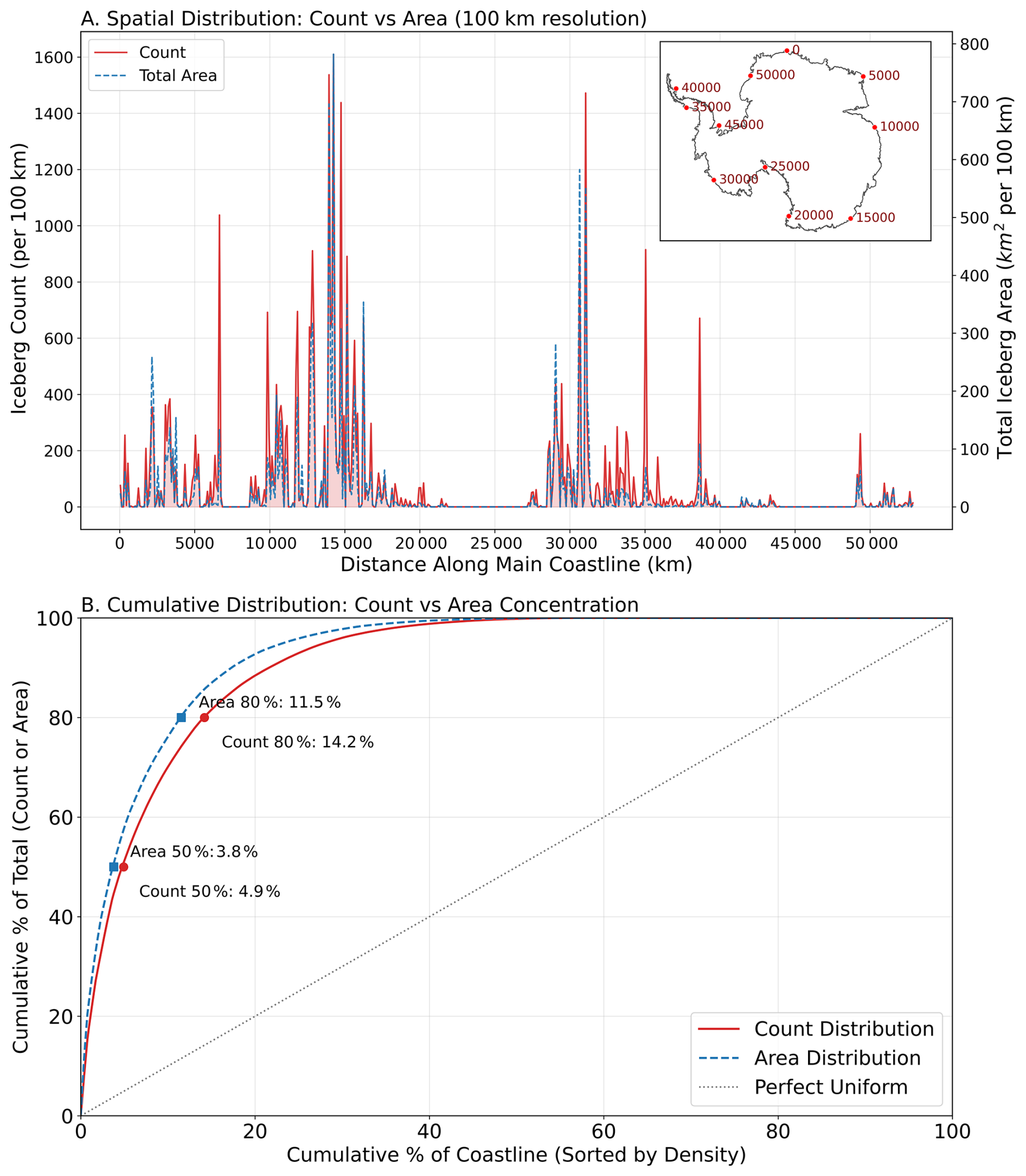
Figure 9 Statistical distribution and spatial concentration of grounded icebergs along the Antarctic coastline. (A) Spatial distribution frequency. The histogram shows the number of grounded icebergs aggregated within 100 km segments along the primary Antarctic coastline. The inset map illustrates the reference coastline, with red markers indicating the cumulative distance (km) measured from 0° longitude, providing geographic context for the x-axis. (B) Cumulative distribution (Lorenz-style curve). The curve quantifies the degree of spatial clustering by plotting the cumulative percentage of grounded icebergs against the cumulative percentage of coastline segments, ordered by iceberg density. The dashed grey line represents a perfectly uniform distribution, for reference.

5 Discussion

5.1 Scientific Significance and Implications

The primary contribution of this study is the establishment of the first high-resolution, circum-Antarctic dataset of grounded icebergs around Antarctica, based on Sentinel-1 SAR imagery. By integrating deep learning-based detection with a multi-temporal identification algorithm, we successfully mapped the distribution of 39 619 stationary icebergs across the entire continental shelf. Crucially, we integrated high-resolution fast ice maps to partition these targets into high-confidence grounded icebergs (located in open water) and fast ice entrapped candidates. This novel classification partially resolves the ambiguity between grounding and fast ice immobilisation, revealing macroscopic distribution patterns previously obscured due to observational limitations. This achievement directly addresses a critical gap in current research on the Antarctic coastal cryosphere: the lack of automated methods for identifying grounded icebergs. Previous studies have largely relied on manual interpretation, which is restricted to specific regions or time periods and is unable to capture dynamic features at the circum-Antarctic scale (e.g., Li et al., 2020; Kostov et al., 2026).

Due to challenging background conditions caused by heterogeneous sea ice and textural similarities, icebergs smaller than 0.1 km² are easily missed by conventional SAR thresholding methods or earlier machine learning models (e.g., Wesche and Dierking, 2015; Barbat et al., 2021; Evans et al., 2023). For instance, while the unsupervised clustering approach by Evans et al. (2023) achieved automated detection, it faced challenges with sub-kilometre icebergs (Class A1, <1 km²), reporting a mean Precision of 0.619 and an F1 score of 0.678 due to high false positive rates in complex environments. In contrast, our deep learning framework demonstrates superior feature extraction capabilities for these small targets, achieving a Precision of 0.8652 and an F1 score of 0.8613. Furthermore, our approach surpasses the detection limit of previous studies (<0.04 km², e.g., Chen et al., 2026), reducing the minimum detectable iceberg size to 0.016 km². This improvement effectively mitigates interference from seasonal sea ice cover variations and complex sea conditions, maintaining high detection stability across most of the year and under a wide range of environmental conditions.

The dataset generated in this study provides a high-precision spatial foundation for analysing the interactions between grounded icebergs, fast ice, and ocean dynamics (Massom et al., 2001; Porter-Smith et al., 2021; Fraser et al., 2023). The spatial distribution confirms that high-density clusters of grounded icebergs are predominantly constrained by shallow bathymetry, typically accumulating on continental banks downstream of ice shelf calving fronts. From an ecological perspective, these dense iceberg clusters are not merely physical barriers but also hotspots of biogeochemical cycling (Duprat et al., 2016; Lucas et al., 2025) and freshwater input (Olivé Abelló et al., 2025). Grounded icebergs stabilise the surrounding sea ice (Fraser et al., 2023), which serves as an important habitats for plankton, sea ice algae, and benthic organisms (Arrigo, 2016; Meiners et al., 2018; Bett et al., 2020). At the same time, the release of iron from iceberg meltwater constitutes a key limiting factor for primary productivity along the Antarctic coast (Herraiz‐Borreguero et al., 2016). In contrast to individual large icebergs, the numerous tiny icebergs identified in this study collectively contribute a larger total surface area (53.90 % of the overall area) and exhibit higher perimeter-to-area ratios. These characteristics indicate that they may play a greater role than previously recognised in nutrient release and in enhancing local stratification (Duprat et al., 2016; Lucas et al., 2025).

Our study reveals the predominance of “tiny icebergs” (<1 km²) within the grounded iceberg population, accounting for 92.6 % of the total. Grounded icebergs are considered key anchoring points for Antarctic fast ice (Massom et al., 2001; Fraser et al., 2023). Previous studies have largely focused on the blocking effects of small to medium icebergs on fast ice (e.g. Li et al., 2020), but the high-density clusters of tiny icebergs revealed in this study suggest that such a “granular” distribution may create a more refined and stable “picket fence effect”. This indicates that, although individual small grounded icebergs cover only a limited area, their large numbers and widespread presence in shallow waters allow them to play a notable anchoring role in the maintenance of fast ice.

Recent dynamical modelling supports the physical viability of these smaller anchors; Kostov et al. (2026) demonstrate that sediment resistance acts as the primary decelerator against atmospheric drag. This resistive force enables even smaller grounded features to withstand strong wind forcing and maintain their position for extended periods, thereby underpinning the stability of this micro-scale “picket fence”. Collectively, these high-density clusters may effectively increase friction along the coastal boundary, restricting the drift and export of sea ice, while physically dissipating the kinetic energy of offshore floes and swell (Massom et al., 2001; Bett et al., 2020).

However, this stabilising mechanism is geographically highly heterogeneous. The finding that 50 % of grounded icebergs are concentrated along only 4.9 % of the coastline, while 80 % occupy just 14.2 %, implies that the Antarctic “picket fence” functions less like a continuous wall and more like a series of discrete, high-intensity structural nodes. This extreme spatial inequality suggests that the stability of circum-Antarctic fast ice may disproportionately depend on these specific “hotspot” regions.

This stability mechanism, which relies on both the numerical dominance of tiny icebergs and their high local concentration, may indicate a unique sensitivity of the Antarctic coastal system to climate change. While their keel depths can be substantial due to potential overturning, tiny icebergs possess considerably lower total mass and thermal inertia compared to large tabular icebergs. Consequently, they are more susceptible to rapid volume loss, disintegration, and subsequent “ungrounding” in response to ocean warming. This implies that even subtle perturbations in environmental conditions within these limited critical zones could lead to the rapid disintegration of this “micro-scale picket fence”, potentially triggering abrupt changes in the stability of fast ice through non-linear processes. In the context of the recent sharp decline in Antarctic fast ice extent (Fraser et al., 2023; Abram et al., 2025; Doddridge et al., 2025), understanding this mechanism is particularly important. Our data suggest that subtle changes in the distribution of grounded icebergs may, through this non-linear collective effect, directly modulate the stability of fast ice and the formation potential of polynyas (Nakayama et al., 2014; Olivé Abelló et al., 2025).

5.2 Limitations

Although this study successfully constructed a circum-Antarctic grounded-iceberg dataset, several limitations remain in relation to data annotation, algorithmic adaptability, and environmental interference, all of which should be taken into account in subsequent applications and analyses.

The construction of a pan-Antarctic mosaic necessitates the integration of heterogeneous SAR data, introducing spatial and radiometric inconsistencies. To achieve complete coastal coverage, this study combines IW and EW modes. While this strategy maximises spatial coverage, the integration of different modes leads to spatially variable detection sensitivities. In our study, the EW mode demonstrated stronger detection capabilities compared to the IW mode, resulting in non-uniform performance baselines across different continental sectors. However, we note that this discrepancy is primarily driven by data availability and model training biases rather than the inherent physics of the SAR modes. Our deep learning model was trained on a dataset primarily composed of EW imagery. Furthermore, due to data availability, the mosaic utilises varying polarisation channels, primarily co-polarisation and cross-polarisation. Iceberg–ocean contrast differs between polarisations, and cross-polarisation typically provides superior contrast over co-polarisation. Consequently, the model’s segmentation sensitivity fluctuates across different orbital swaths, potentially introducing bias in regional iceberg density estimates.

In terms of data annotation and the detection of very small targets (<25 pixels), both manual mask labelling and automated model prediction face substantial challenges. Extremely small icebergs (<25 pixels) are often embedded within complex sea ice-dominated backgrounds, leading to ambiguous boundary definition. For targets smaller than 10 pixels in particular, local high backscatter caused by strong winds or wave breaking (sea clutter) is almost indistinguishable from real icebergs in terms of brightness (Marino et al., 2016). The close similarity in backscatter intensity introduces uncertainty into manual interpretation, which inevitably injects label noise into the training dataset. It also reduces the model’s discriminative power during inference, making it difficult to eliminate false positives under complex sea conditions. In addition, in extremely dense iceberg regions, the model occasionally merges closely adjacent icebergs into a single entity, potentially resulting in slight underestimation of the local iceberg count.

A further limitation of the spatiotemporal identification algorithm emerges in regions characterised by an extreme density of small, highly mobile icebergs, such as the Bellingshausen Sea. In these highly congested areas, coincidental spatial overlap introduces an unavoidable source of false positives. Even when the independent single-frame detection and multi-temporal tracking algorithms are functioning nominally, in some cases these may have been misidentified as grounded when different small drifting bergs sequentially occupied overlapping positions between the 12 d SAR passes. Because these transient targets coincidentally satisfy the geometric and spatial proximity thresholds required for trajectory continuation, the algorithm inherently interprets them as a single stationary entity.

A specific uncertainty arises from the reliance on bathymetric constraints for false positive removal. While the application of a 1000 m depth threshold effectively eliminates spurious detections in deep open-ocean regions because grounding is physically impossible, it implies that similar detection artifacts likely persist in the shallower continental shelf regions. False positives caused by complex sea ice background texture, stationary fast ice ridges, or immobilised floating icebergs share identical radiometric characteristics in both deep and shallow waters. However, our filtering framework actively mitigates these across both regimes, with deep and shallow waters accounting for approximately 46 % and 54 % of the eliminated targets, respectively (Table 7). In the potential grounding zone (<600 m), where depth criteria alone are insufficient, we utilise a combined area and SIC strategy to manage complex sea ice backgrounds. This approach is physically justified: in shallow waters, icebergs immobilised by sea ice are highly likely to be genuinely grounded if they are sufficiently large. Our area thresholds inherently retain these larger icebergs, which possess deeper keels capable of interacting with the seabed, while effectively filtering out smaller sea ice artifacts. Although a minor proportion of unquantifiable false positives persists, particularly in areas with strong backscatter associated with large-scale deformed fast ice (especially multi-year fast ice), this dual approach improves the robustness of final dataset. However, we also acknowledge that inaccuracies or coarse spatial resolutions in these underlying auxiliary datasets (such as IBCSO bathymetry or AMSR2 SIC) could theoretically lead to the erroneous exclusion of truly grounded icebergs, thereby producing false negatives.

Regarding the distinction between grounding and entrapment (i.e., immobilisation by the fast ice itself), reliance on auxiliary datasets introduces specific uncertainties. In previous methodologies, distinguishing grounded icebergs from floating ones immobilised by landfast sea ice was a primary challenge, as both share identical radiometric characteristics. To address this, we integrated high-resolution fast ice maps to partition targets into three categories (Sect. 3.4), thereby effectively isolating high-confidence grounded icebergs in open water. However, this classification strategy implies that the reliability of the grounding status for “Inside” and “Partial” targets is inherently dependent on the accuracy and temporal synchronisation of the input fast ice mask. Any potential errors in the fast ice boundary definition could lead to misclassification of the grounding status for these specific candidates. Consequently, while the “Outside” category represents a robust baseline of truly grounded targets, “the Inside” and “Partial” categories should be interpreted with consideration of the surrounding fast ice context.

Regarding the identification algorithm, although Hu invariant moments (Hu, 1962) are generally robust for shape-based matching, their stability decreases when applied to tiny icebergs (<25 pixels). Owing to the limits of spatial resolution, shape descriptors for such small objects are easily affected by pixel-level quantisation errors, reducing the reliability of trajectory association. Similarly, in densely packed iceberg clusters, the frequent merging and separation of neighbouring icebergs can cause unstable variations in the segmentation results. These fluctuations can lead to abrupt changes in key object features (such as area and centroid), thereby disrupting the continuity of feature-based trajectory matching.

The temporal inconsistency of the data acquisition introduces environmental variability. As the dataset is a composite of acquisitions spanning late summer to early autumn, specifically February to April, environmental conditions are not uniform. Acquisitions from February may still be influenced by residual surface melt and wet snow. These conditions reduce the radar contrast between icebergs and the background, thereby lowering detection scores, as evidenced by the drop in F1 score for December to 0.8472 compared to the annual average of 0.9121 (Table 3). Conversely, images acquired in the colder transition period (March and April) may contain patches of residual high-backscatter multi-year fast ice. These features can be misclassified as icebergs due to their similar texture. Although we primarily targeted the March transition period to mitigate these extremes, this temporal spread implies that the background noise varies geographically across the dataset. Consequently, precision in specific regions may fluctuate, as indicated by the March precision of 0.8526 shown in Table 2.

Finally, due to the tile-processing strategy and the limited spatial context captured by the model, the ResUNet architecture still faces challenges when handling large and giant icebergs. Although it outperforms previous methods for detecting small to medium-sized icebergs, icebergs larger than the field of view of a single sub-image are difficult to segment completely. The lack of global contextual information prevents the model from perceiving the continuous geometry of an object that spans multiple tiles, which may lead to fragmented segmentation or missing boundaries in large-scale contours.

5.3 Future work

Future research will aim to fully exploit the scientific value of this dataset while addressing the limitations identified in the present study. First, multi-source remote sensing data fusion can be further advanced by integrating altimetry datasets (such as the Ice, Cloud, and land Elevation Satellite-2 – ICESat-2), extending the current two-dimensional monitoring to three-dimensional volume estimation, and facilitating draft estimation (Markus et al., 2017). While fully reconstructing the 3D surface morphology of individual icebergs is challenging given the sparse nature of altimetry profiles, fusing these draft estimations with 2D SAR boundaries remains highly valuable for statistical volume approximations. This approach facilitates quantifying freshwater flux from melting, thereby improving understanding of its impacts on local salinity, ocean circulation, and polar coastal ecosystems (Olivé Abelló et al., 2025). Looking ahead, next-generation swath-mapping missions like the Earth Dynamics Geodetic Explorer (EDGE) promise to overcome these profiling limitations, providing contiguous coverage that will enable true 3D morphological reconstructions (Garvin et al., 2026). In addition, multi-source data fusion may enhance monitoring across iceberg scales, from tiny to giant, providing a reliable basis for long-term dynamic databases and predicting climate-driven responses.

Second, a long-term dynamic monitoring system can be established using historical SAR archive data to reconstruct a decadal record of grounded icebergs across Antarctica, thereby revealing their long-term spatiotemporal evolution under a warming climate (Fraser et al., 2023; Doddridge et al., 2025). Building on this, process-based studies of the iceberg–sea ice–ocean system can be conducted by integrating high spatiotemporal resolution sea ice drift and ocean forcing data, quantifying the thermodynamic control of grounded iceberg distributions on fast ice stability (Massom et al., 2001; Fraser et al., 2023) and polynya formation (Nakayama et al., 2014), and exploring their potential cascading effects on polar coastal ecosystems (Arrigo, 2016; Meiners et al., 2018). However, accurate discrimination between stationary and truly grounded icebergs becomes more difficult prior to 2021, when summertime fast ice extent was far higher than in recent years (Abram et al., 2025).

Finally, to further improve model performance under complex conditions, future work could incorporate global contextual information (referring to the broader spatial context beyond the current 250×250 pixel sub-image input in this study) into the modelling framework. This wider view serves two critical purposes. It allows the model to perceive the continuous geometry of larger icebergs that span across multiple tiles, thereby preventing fragmented segmentation. In addition, integrating a wider spatial context provides richer environmental constraints, helping the model to recognise large-scale background interference (such as extensive patches of severe sea clutter or heavily deformed fast ice), allowing it to better distinguish true targets from false signals (including those indistinguishable by bathymetry) in cases where tiny icebergs are highly similar to background interference, such as sea clutter or residual fast ice.

6 Code availability

The code and datasets supporting this study are available on GitHub at https://github.com/kj0703/Antarctic-Grounded-Iceberg-Detection (last access: 20 August 2026) and are permanently archived on Zenodo at https://doi.org/10.5281/zenodo.19228332 (Jiao and Lohse, 2026).

7 Data availability

The grounded iceberg dataset is publicly available at https://doi.org/10.25959/54sx-pt47 (Jiao et al., 2026). Detailed field descriptions are provided in Table 1.

8 Conclusions

In response to the current lack of automated monitoring of grounded icebergs across Antarctica, this study introduces an automated detection framework that integrates a proposed ResUNet deep-learning network with a multi-temporal identification algorithm. The method demonstrates strong robustness against signal interference in complex coastal environments, achieves stable detection performance (F1 >0.91), and successfully reduces the minimum detectable iceberg size to 0.016 km². Using Sentinel-1 SAR imagery, we construct the first high-resolution, continent-wide dataset of grounded icebergs in Antarctica.

Statistical analysis shows that almost 40 000 stationary icebergs were identified along the Antarctic coastline in March 2025 (67.4 % of which were classified as high-confidence grounded icebergs), with tiny icebergs (<1 km²) dominating numerically and accounting for 92.6 % of all grounded icebergs. Spatial patterns further reveal that these high-density iceberg clusters are concentrated mainly on shallow continental shelves and along the actively disintegrating fronts of ice shelves, forming complex and discontinuous “grounded iceberg chains”. Overall, these features are distributed along 56.52 % of the continental coastline, with 80 % concentrated within just 14.2 % of the coastline. This finding builds on earlier studies that predominantly examined medium and large icebergs, providing further evidence that aggregations of tiny icebergs may play a more important role than previously recognised in maintaining fast ice and regulating biogeochemical processes through a “picket fence effect”.

The dataset provides a new high-precision benchmark for quantifying the Antarctic ice–ocean interaction network, and it establishes a robust technical foundation for reconstructing long-term iceberg dynamics from historical imagery and projecting their responses to climate change.