POPE: an annual global half degree emission inventory for PFAS 1950–2020

This study presents a global multi compartment Persistent Organic Pollutant Emissions model and inventory: POPE. The model computes temporally and spatially resolved model ready emissions for 23 Per- and Polyfluoroalkyl Substances (PFAS). It focuses on some of the most widely used substances and distinguishes between emissions to air and emissions to water. POPE covers the time span from the first industrial scale production in 1950 up until 2020 on an annual basis on a grid with 0.5° resolution.

The POPE model distributes estimated total PFAS emissions in space and time based on several data sets such as the E-PRTR, NACE and US-EPA FRS in combination with socio-economic data as population and GDP complemented by estimates for individual point sources, such as industrial sites and airports, whereby the source activity is dependent on regional changes in production volumes, usage quotas, and recapturing efficiency over time. It includes emissions by industrial production, diffuse emissions through usage and disposal of consumer products, secondary emissions from the reaction of precursors, and emissions by firefighting exercises on airports using Aqueous Film Forming Foams (AFFF).

It is demonstrated that the POPE emission inventory is compatible with current global emission estimates, and temporal and spatial variability of the emissions is explored. A comparison of independent measurements with modelled river concentrations based on the POPE emission inventory is provided.

The POPE emission inventory is meant to be used as input for atmospheric and marine chemistry transport models, eventually allowing to assess the environmental fate of PFAS. POPE can be used to create hypothetical future emission scenarios, enabling model based predictions which can inform policy decisions. This is important given that even with a theoretical global fade-out of PFAS production, significant legacy pollution is still to be expected.

The POPE emission inventory for PFAS is publicly available in GEIA's (Global Emission InitiAtive) ECCAD data portal: (https://permalink.aeris-data.fr/POPE, last access: 3 June 2025) or including the source code at zenodo (https://doi.org/10.5281/zenodo.12783504, Simon, 2024).

1 Introduction

Per- and polyfluoroalkyl substances (PFAS) constitute a group of substances known for their high persistence (Guelfo et al., 2021; Cousins et al., 2020), toxicity (Post et al., 2012; Vierke et al., 2012), and bioaccumulative nature within the food chain (Conder et al., 2008; Martin et al., 2003). This characteristic leads to long-term exposure of human populations, raising significant concerns for both human health and the environment (Buck et al., 2011). Despite their known adverse effects, PFAS are widely used due to their stability and their water-, oil-, and dirt-repelling properties, finding applications in water and dirt repellent coatings, food-packaging, outdoor apparel, furniture, firefighting foams, aerosol propellants, and heat transfer fluids. (Glüge et al., 2020; OECD, 2004) However, this very stability contributes to their high risk for humans and the environment (Kirk et al., 2018). National and international effort has been made to regulate PFAS (Brennan et al., 2021b; UNEP, 2020; EC, 2022) but is constrained by competing interests and limited understanding. Therefore, understanding the behavior, fate, and effects of PFAS in the environment is crucial for mitigating their potential harm to human health and the ecosystem.

In addition to environmental measurements (Kannan et al., 2002; Mclachlan et al., 2007; Cousins et al., 2011; De Silva et al., 2021), numerous numerical transport modeling studies of PFAS have been conducted to investigate and comprehend the fate of PFAS. These studies encompass global analyses, such as those conducted by Stemmler and Lammel (2010), Armitage et al. (2006), and Thackray and Selin (2017). Some studies focus on specific regions like Yarwood et al. (2007) or water bodies like the Danube, as demonstrated by Lindim et al. (2015b), while others concentrate on specific PFAS emitters, as exemplified by Shin et al. (2011).

A critical initial step in any transport modeling study is a temporally and spatially resolved emission inventory. However, for many PFAS, such data is either unavailable or lacks adequate attribution, resolution or spatiotemporal coverage. Several widely used estimates of global emissions for groups of PFAS, such as perfluoroalkyl carboxylic acids (PFCAs), have been proposed by Wang et al. (2014a), Prevedouros et al. (2006), and Armitage et al. (2009). Nevertheless, these global estimates are not spatially resolved. To tackle this problem, numerical modeling studies distribute PFAS emissions based on various spatial proxies, such as NO_x emission maps (Thackray and Selin, 2017). However, many of these modeling attempts do not allow for differentiation between emission sources, precursor reactions, or emissions to different environmental compartments. This differentiation, especially between emissions to the atmosphere and surface waters, is crucial for global long-range transport and multi-compartment modelling (Bieser and Ramacher, 2021; Holland et al., 2020).

Motivated by this gap in current research, the present study introduces the Persistent Organic Pollutant Emission model (POPE) and its associated emission inventory. POPE aims to refine existing inventories to provide a global, consistent, scenario-capable (Matthias et al., 2018) emission model for PFAS emissions. The POPE model distinguishes between emissions released to water and emissions released to air, using a half-degree resolution grid and a temporal resolution of one year, spanning the years 1950 until 2020.

Building upon the extensive research conducted on widely used PFAS, such as Perfluorooctanoic Acid (PFOA) and Perfluorooctanesulfonic Acid (PFOS), POPE extends the knowledge and methods used to distribute these compounds in space and time to other PFAS for which data is more limited. This includes other PFAS from the groups of PFCAs and perfluorosulfonic acids (PFSAs), as well as precursors that react under environmental conditions to form PFAS. Additionally, emerging compounds, such as HFPO-DA and ADONA, used as replacement for phased-out legacy compounds, are considered. POPE distributes known global inventories using proxies and socioeconomic data supported by field measurements, while also incorporating point sources such as airports and industrial sites.

The employed methodology begins with a discussion of global total emissions based on available data. This is followed by a description of the spatial disaggregation and temporal inter- and extrapolation applied in the POPE model. Each section is further divided based on emission sectors. Looking at the resulting POPE emission inventory, the consistency of POPE's global total PFAS emissions with other works is assessed. The subsequent chapter presents the spatial distribution of the POPE emission inventory and its global trends. Afterwards, the POPE emission inventory is evaluated using the Hydrological Discharge (HD) model (Hagemann et al., 2020) and several studies on PFAS river concentrations. Finally, the resulting POPE emission inventory is discussed with regard to its performance and data gaps.

2 POPE Inventory Construction

2.1 Modeled PFAS species

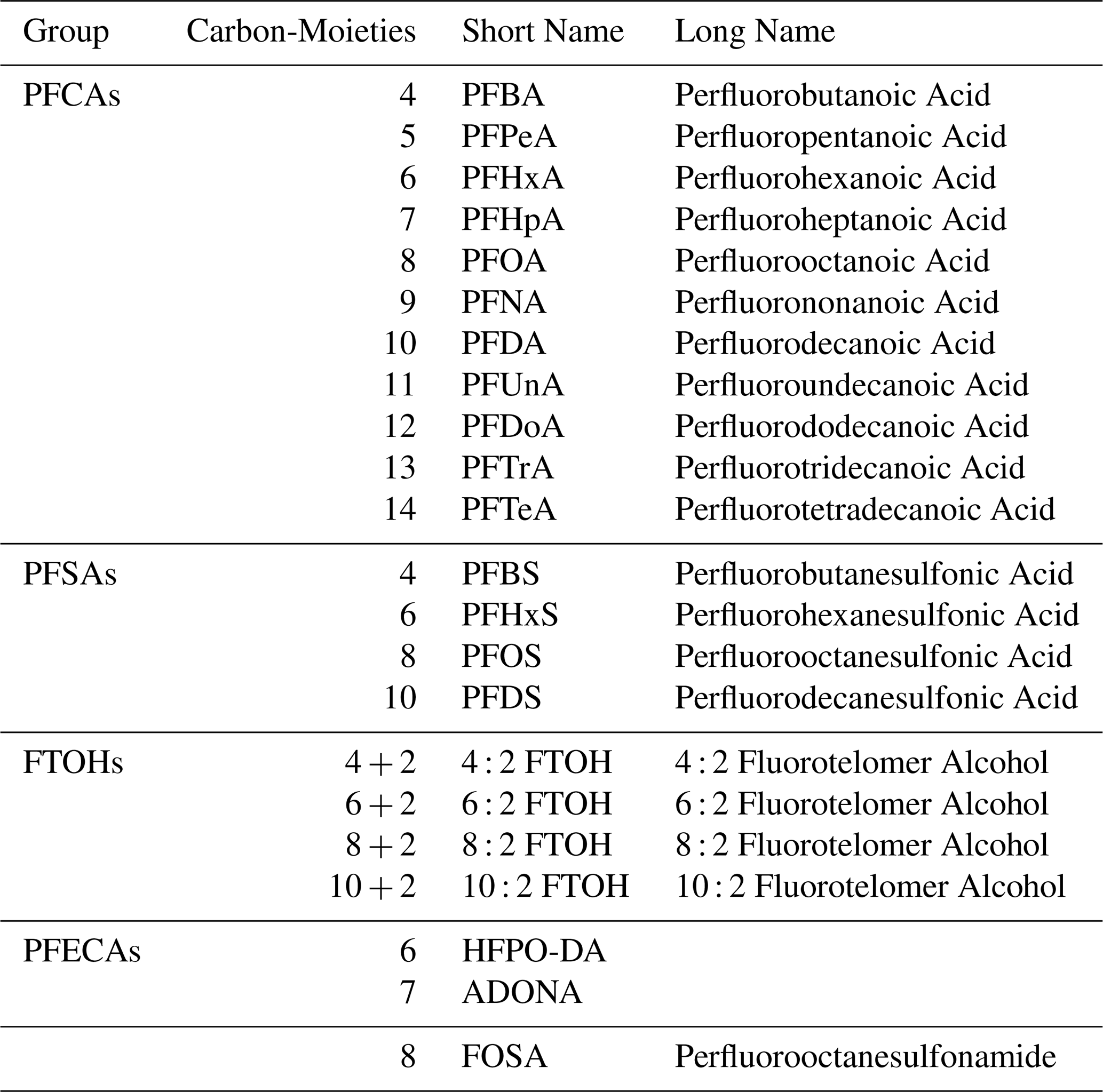
The POPE (Persistent Organic Pollutant Emission) inventory provides global gridded emissions for 23 individual per- and Polyfluoroalkyl Substances (PFAS). POPE covers emissions to air and water for the time span 1950–2020. The 23 PFAS (Table 1) considered in POPE are:

• 11 Perfluoroalkyl carboxylic acids (PFCAs)

• 4 Perfluorosulfonic acids (PFSAs)

• 5 Fluorotelomer alcohols (FTOHs)

• Perfluorooctanesulfonamide (FOSA)

• 2 replacement compounds (HFPO-DA and ADONA)

The chosen species are those currently regulated under Annex A and B of the Stockholm Convention (UNEP, 2020) and those about to be regulated by the European Commission (EC, 2022) excluding the replacement compound “C6O4” due to the limit of available data. Additionally, emerging replacement compounds hexafluoropropylene oxide dimer acid (HFPO-DA, in its ammonium salt form also known under the brand name Gen-X) and 4,8-dioxa-3H-perfluorononanoic acid (in its ammonium salt form known under the brand name ADONA) were included due to their anticipated future importance (Joerss, 2020; Munoz et al., 2019). A detailed list of all included compounds is given in Table 1

Table 1 PFAS included in the POPE emission inventory.

2.2 Emission and proxy datasets used by POPE

POPE uses several available datasets for direct and indirect emission estimation. These include aggregated emission estimates based on the total global emission inventories of Wang et al. (2014a), Prevedouros et al. (2006), and Armitage et al. (2009). Additionally several data sets of known point sources or regional datasets as well as aggregated emissions for regional compartments are included.

POPE temporally and spatially downscales the aggregated PFAS emissions into a global 0.5 × 0.5° gridded annual emission dataset suitable for chemistry transport models (CTMs). The downscaling is based on publicly available socioeconomic data sets. Besides this, time series of environmental observations of PFAS are used to estimate levels and trends in source activity.

POPE makes use of:

•  

  Global emission datasets

  • Global emission inventory for PFCAs 1951–2004 by Prevedouros et al. (2006)

  • Extension of the emission inventory by Prevedouros et al. with estimations considering distribution across large spatial scales and environmental compartments by Armitage et al. (2009)

  • Global emission inventory for PFCAs (C4–C14) 1951–2030 partly building on Wang et al. (2014b), partly building on Prevedouros et al. (2006)

•  

  Point source emission registers

  • European pollutant release and transfer register (E-PRTR) containing locations of relevant industries in Europe, 2007–2020 (EC, 2023)

  • Nomenclature statistique des activités économiques (NACE) Rev. 2 providing sub-national data on number of sites and of employees for relevant industries in Europe, 2008 (Eurostat, 2025)

  • Facility Registry Service (FRS) of the United States Environmental Protection Agency providing relevant locations in the United States, 2020 (U.S. EPA, 2023)

•  

  Individual emission data for large point sources

  • Purchasing records, production volumes and estimated losses for the Dupont Plant Parkersburg West Virginia by Paustenbach et al. (2007a)

  • Multiple fluoropolymer production sites globally (Will et al., 2005; Wang et al., 2014a; Prevedouros et al., 2006)

  • Production volumes and used PFAS for several plants in Europe (Dalmijn et al., 2023)

  • Swedish airports (Ahrens, 2009; Filipovic et al., 2013b)

•  

  Local emission data

  • Large Emitters in Sweden (OECD Environment Directorate, 2018)

  • Emitters in the Danube watershed (ICPDR, 2003)

  • Emission load in a boreal watershed (Filipovic et al., 2015)

  • Emissions in European rivers in 2008 (Loos et al., 2009)

  • Emissions to the Baltic Sea (Filipovic et al., 2013)

  • Emissions caused by US WWTPS (Hamid and Li, 2016)

Furthermore POPE uses multiple datasets for the distribution and transport of known emissions, These are:

•  

  Socio-economic datasets

  • Population density data 1950–2020 (Chambers, 2020)

  • Georeferenced GDP data 1990–2015 (Kummu et al., 2018)

  • Global dataset of airport designations 2020 (ICAO, 2014)

  • US WWTP runoff 1930–2000 (Hale et al., 2015)

•  

  Environmental datasets

  • Global Soil Wetness Project Phase 3 forcing data, 1950–1978 (Dirmeyer et al., 2006)

  • WATCH Forcing Data based on ERA5 re-analysis 1979–2020 (Cucchi et al., 2020)

2.3 Speciation

The relevant data sets for each used substance vary, based on the relevant emission sectors and the availability of specific data and its associated uncertainty. We differentiate 4 general approaches:

• Legacy compounds (PFOA and PFOS)

• PFCAs and PFSAs

• FTOHs

• Replacement compounds (Gen-X, ADONA and FOSA)

The only common data sources impacting all substances are population and GDP data. The relative contribution to emissions varies from substance to substance relating to their specific fraction of industrial vs consumer emissions. As the relative uncertainty in population and GDP data is small compared to other relevant data it does not feed into upper and lower bound scenarios.

PFOA and PFOS share a specific role of being the most researched in their respective groups (Wang et al., 2017b). Therefore there are direct estimates of sector specific emissions available, allowing a bottom up approach. This allows them to be independent of calculated totals in other works, making a comparison possible. All given data sets are used depending on the region and emission sector, explained in detail in the next sections. The given bounds in these datasets feed directly into the lower and upper bounds of POPE. Where emissions are calculated by a combination of multiple data sources, given uncertainties are combined by a Gaussian propagation of uncertainty.

PFCAs and PFSAs are built on total emissions estimates distributed based on datasets and patterns of PFOA and PFOS, respectively. They inherit assumed group-specific properties, such as loss fractions and usage rates, as well as the temporal characteristics. The uncertainties in PFOA and PFOS calculations also feed in the bounds of their groups, multiplied by the range of possible totals.

FTOHs, on the other hand, have no datasets with individual point sources available and are therefore distributed as a per-group approach. 8 : 2-FTOH is exemplary for the group, where the emissions of all other FTOHs are scaled according to their relative production volumes. As FTOHs can function as precursors to PFCAs, they are not dependent on PFCA emissions to avoid circular dependencies. The upper and lower bounds are made up of the uncertainty of the totals, coupled with the calculated distributional error by the industrial approach of Sect. 2.5.1.

The replacement compounds Gen-X, ADONA and FOSA follow a substitutional approach, assuming continued production of related products with a range of replacement factors given in Sect. 2.4.2. The replacement factor of the latter two is based on the associated industrial process, while FOSA is associated to PFOS concentrations by environmental measurements. The associated uncertainty is obtained by Gaussian error propagation based on the range of replacement factors and the calculated error already present in the substituted substance.

2.4 Emission Sectors

The produced emission dataset distinguishes emissions for each PFAS or precursor species (Table 1) for each of the 6 source sectors (Table 2). The industrial manufacturing sector dominates the total emissions for many PFAS. The single largest emitter of PFAS is fluoropolymer production which is estimated to account for over 70 % of the total global PFCA emissions from 1951 to 2004 (Prevedouros et al., 2006). It is assumed to be the largest contributor to the global inventory of PFCAs and PFSAs (Cousins et al., 2011; Lim et al., 2011) pre 2001 and might be the largest source for their replacements like PFECAs and FOSA in the future (Wang et al., 2013; Scheringer et al., 2014). Apart from fluropolymer production, other industries like textile manufacturing, coating of surfaces or electronics are important industrial emission sources. As a smaller but locally very significant source, Aqueous Film Forming Foams (AFFF) used for airport firefighting and firefighting excercises is also taken into account.

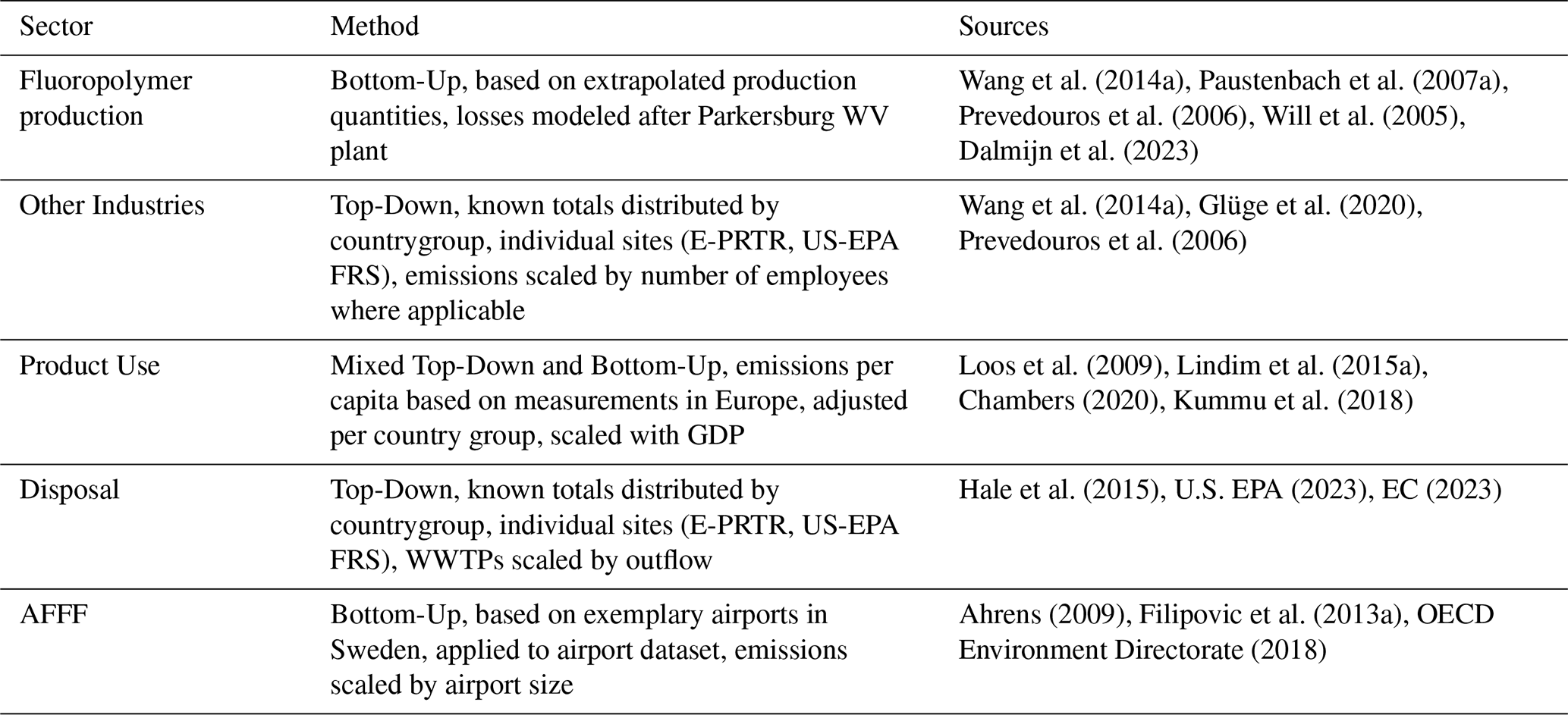
POPE employs different methods for the emission estimation of each individual sector. Table 2 gives an overview of the used methods and the data sources for each sector.

Wang et al. (2014a)Paustenbach et al. (2007a)Prevedouros et al. (2006)Will et al. (2005)Dalmijn et al. (2023)Wang et al. (2014a)Glüge et al. (2020)Prevedouros et al. (2006)Loos et al. (2009)Lindim et al. (2015a)Chambers (2020)Kummu et al. (2018)Hale et al. (2015)U.S. EPA (2023)EC (2023)Ahrens (2009)Filipovic et al. (2013a)OECD Environment Directorate (2018)

Table 2 Overview of the sectors in POPE with the employed methods and data sources to obtain the respective emission estimations.

In the following sections, we will describe the individual sectors in detail and explain how annual total emissions were estimated for each of them.

As a general approach POPE estimates annual total emissions of a compound for a given single industrial point-source or region. Production emissions are estimated based on production volumes, which are modulated by changing activity rates, loss fractions, and compartmental coefficients where applicable as discussed in Sect. 2.4.1. Where the data for this bottom-up approach is not sufficient, available regional emission estimates are distributed. For the US and Europe that is mostly based on known registered sites with respect to their number of employees, if available, as shown in Sect. 2.4.2. For most other countries diffuse emissions are distributed by population and GDP as a proxy illustrated in Sect. 2.4.3. The same applies for product use and dispoal unless data on Waste-Water-Treatment-Plants (WWTPs) or landfills are available. AFFF emissions are estimated by airport size and designation shown in detail in Sect. 2.4.4.

2.4.1 Fluropolymer production

Fluoropolymer production is the most important source for many PFAS and thus receives special attention in POPE. The process is based on the most extensively researched fluropolymer production plant of the company Dupont in Parkersburg, West Virginia and the extensive data published by Paustenbach et al. (2007a).

This data helps to relate available fluoropolymer production volume V found for different plants in economic datasets to actual emissions of PFAS. This is done with two additional factors: a usage rate and a loss fraction. The usage rates c describes how much of the corresponding PFAS is needed per ton of produced Fluoropolymer V. The loss fraction f describes how much of the used PFAS is expected to be lost in the process and to which environmental compartment (air or water) it is emitted.

Building on this, the expected PFAS emission E [kg] is calculated depending on the medium as

$$\begin{array}{}\text{(1)}& E_{\mathrm{medium}}=V\cdot c\cdot f_{\mathrm{medium}},\end{array}$$

with the production volume V [kg], loss-fraction f [–] to the corresponding compartment and the usage rate c [–]. With respect to fluoropolymer production, the individual production volumes of sites are based on multiple sources. Several approximated production volumes for different years are taken from Wang et al. (2014a), Paustenbach et al. (2007a), Will et al. (2005), and Dalmijn et al. (2023). This allows POPE to consider the production of Polytetrafluoroethylene (PTFE), fluorinated ethylene propylene (FEP), Polyvinylidene fluoride (PVDF), and perfluoroalkoxy alkane (PFA) as point sources. PFAS are typically not used as monomers itself but rather polymerization aids. The loss fraction and usage rate are specific to the PFAS used in the production process and the produced fluropolymer. Ususally both are not fixed and depend on the process used, which is not necessarily publicly known for each plant. Wang et al. (2014a), Paustenbach et al. (2007b), and Prevedouros et al. (2006) provide ranges for the usage rate which POPE takes into account for the upper and lower bound emission scenarios.

For the loss fractions different measurements are available (Wang et al., 2014a), with the most extensive study published by Paustenbach et al. (2007a) based on purchasing records. Differences in estimated loss fractions are again used to define higher and lower bound estimates.

2.4.2 Other Industries

Smaller fluoropolymer production plants and other industries are also considered in POPE. Unlike the bigger plants, these are disaggregated via a top down approach. Based on production and emission estimates, PFAS emissions are disaggregated for the following industrial sectors:

• Apparel manufacturing

• Aerospace product and parts manufacturing

• Manufacturing of chemicals and chemical products

• Manufacturing of computer, electronic and optical products

• Semiconductor and other electronic component manufacturing

• Treatment of fibres or textiles

• Manufacturing of furniture

• Motor vehicle and parts manufacturing

• Paint, coating, and adhesive manufacturing

• Manufacturing of paper and paper products

• Resin, synthetic rubber, and artificial and synthetic fibers and filaments Manufacturing

• Manufacturing of rubber and plastic products

• Surface treatment of metals and plastics

• Manufacturing of textiles

Each sector is of varying importance, specific for each compound. The individual estimated contributions with their upper and lower bounds are found in the are found in the uploaded data (https://doi.org/10.5281/zenodo.12783504, Simon, 2024).

The contribution of each sector to the total emissions is based on the estimations by Wang et al. (2014a) and Prevedouros et al. (2006).

As HFPO-DA and ADONA are mainly used as direct replacements (Joerss, 2020; Munoz et al., 2019), their totals are related to the substituted volume of processing aid.

This is done by using fixed replacement factors based on Dalmijn et al. (2023), Gebbink and van Leeuwen (2020), Brandsma et al. (2019), and Zarȩbska et al. (2024) feeding into the upper and lower bound estimates with the arithmetic mean used as the best guess estimate.

It is assumed that the production of related facilities carries on with identical growth factors and loss fractions and with complete substitution with the appropriate replacement. This corresponds to multiplication of the emissions by the replacement factors. The appropriate replacement is chosen based on the associated company. GenX is produced by Chemours (formerly DuPont), whereas ADONA is a 3M/Dyneon product. They can be used as a replacement for PFOA in PTFE production or PFNA in PVDF production.

FOSA is handled differently to all other compounds as no global totals and no production data is available. The total emission is approximated by using measured concentrations and their relation to PFOS as a proxy. This is due to FOSA being a precoursor to PFOS and their uses being very closely related (Pickard et al., 2022). For this purpose water samples and samples in biota are available (Soerensen and Faxneld, 2023; Pickard et al., 2022). The ratios in biota are corrected by dividing them by the bioaccumulation factors calculated by Soerensen and Faxneld (Soerensen and Faxneld, 2023). All measurements are averaged over the respective regions. This gives estimated total FOSA emissions of 2.5 % and 1.1 % of PFOS emissions in Europe and the United States respectively. This would result for example in emissions of 575 kg in Europe or 473 kg in the United States in the best case scenario in 2010.

2.4.3 Product Use and Disposal

The second largest contributor to total emissions of PFAS is the release by PFAS containing products during their life cycle (Pistocchi and Loos, 2009; Glüge et al., 2020). The range of such products, from outdoor jackets and furniture to floor wax and dental floss, is very broad and there is only limited data available on the total usage of these products, their PFAS content, and the associated PFAS loss over time.

The total emissions during lifetime of PFAS containig products in a given area is related to the population of that area (top-down), which in turn gives an estimate of the emissions by product use of one individual. This is eventually used for the local emissions of other areas (bottom-up). Assuming sufficient locality and only slow changes over time, this can be achieved with the total emission load of rivers and the population in their watershed. Similar approaches have been used before, for example by Lindim et al. (2015a). The relation of the river emission load to a corresponding atmospheric load has to be assessed in a second step afterwards.

The total load of a river is calculated by the river runoff and a reliable PFAS concentration measurement at the estuary. This has for example been done for PFOA and PFOS by Pistocchi and Loos (2009) as well as Mclachlan et al. (2007) for major European rivers. Rivers with known major contributors such as PTFE production sites are ruled out, so that the emissions from these are not taken into account twice. Performing a linear and a log-linear regression between population in the watershed and annual PFOA load leads to a PFOA Emission E [µg d⁻¹], depending on the population p according to

$$\begin{array}{}\text{(2)}& E=\mathrm{19.2}{\displaystyle \frac{\mathrm{\mu }\mathrm{g}}{\text{person}\cdot \text{d}}}\cdot p\end{array}$$

for a linear regression and

$$\begin{array}{}\text{(3)}& E=\mathrm{5.1}{\displaystyle \frac{\mathrm{\mu }\mathrm{g}}{\text{person}\cdot \text{d}}}\times {\mathrm{10}}^{-\mathrm{4}}\cdot p^{\mathrm{1.2841}}\end{array}$$

for a log-linear regression. Performing the same for PFOS Emissions E [µg d⁻¹] yields

$$\begin{array}{}\text{(4)}& E=\mathrm{6.4}{\displaystyle \frac{\mathrm{\mu }\mathrm{g}}{\text{person}\cdot \text{d}}}\cdot p\end{array}$$

for a linear regression and

$$\begin{array}{}\text{(5)}& E=\mathrm{3.5}{\displaystyle \frac{\mathrm{\mu }\mathrm{g}}{\text{person}\cdot \text{d}}}\times {\mathrm{10}}^{-\mathrm{4}}\cdot p^{\mathrm{1.0115}}\end{array}$$

The linear regression suggests lower emission values than the exponential regression, therefore POPE uses the linear regression for the lower bound, whereas the log-linear regression is used for the upper bound. As this data is not available for other compounds than PFOA and PFOS, it is assumed that the product use of PFCAs and their replacements scale similarily with poulation as PFOA, whereas PFSAs and their replacement follow the trend of PFOS. In both cases the prescribed total is conserved.

2.4.4 Aqueous Film Forming Foams

Aqueous Film Forming Foams are relevant for firefighting training and operational use on airports. As airport emissions play a minor role in the total inventory, they are typically considered for global emissions but not spatially resolved. On a regional/local scale on the other hand, airport firefighting emissions might still dominate PFAS emissions (Ahrens et al., 2015). This is mainly due to the fact, that especially in remote regions and low population density areas air transportation of passengers and goods becomes relatively more important, as it is for example the case in Sweden (Hansson et al., 2016).

The POPE model focuses on bottom-up emission estimations of individual airports. The 60 biggest airports worldwide are handled individually while all other relevant airports are categorized in 5 categories where each category gets assigned a single emission load.

Available Data regarding the PFAS emissions of airports includes measurements at Arlanda Airport, Stockholm, Sweden by Ahrens et al. (2015), measurements near a military airport near Stockholm by Filipovic et al. (2015), and the estimated total PFOA emission of airports in Sweden, based on the PFAS-content and their total use of PFAS-based firefighting foam (Hansson et al., 2016).

The regulations of the International Civil Aviation Organization (ICAO) requires the number of fire-departments, firefighting trucks or firefighters to scale among other factors with the number of flights an airport receives (ICAO, 2014). Therefore the amount of firefighting foam used, and with that, the volume of PFAS emitted, is assumed to scale with the number of firefighters employed using AFFF for their regular exercises. Thus, the PFAS emission of the 60 biggest airports worldwide is scaled in relation to the number of flights per year, relative to Arlanda Airport.

Data on the yearly number of flights is not available for every airport worldwide. For the estimation of emissions of smaller airports, this work makes use of the locations of airports according to the IATA and ICAO Databases (ICAO, 2014) and the report by the Nordic Council of Ministers (Goldenman et al., 2019). The ICAO dataset categorizes airports in 3 different size classes. Airports are differentiated as of primarily civilian or primarily military use by designation, since military airports are shown to reach nearly 3 times the emissions of civilian airports of a similar size (Linderoth et al., 2016). All small civilian airports are dropped due to their insignificance. As large civilian and military airports are handled individually, this leaves estimates for medium civilian, small military and medium military airports to be considered. Out of circa 60 000 airports, heliports and landing fields in the data set circa 6500 are included.

Following Ahrens et al. (2015) the medium civilian airport emissions are obtained by subtracting the emissions of Arlanda Airport from the total PFAS emissions attributed to civilian airports in Sweden as estimated by Hansson et al. (2016) and dividing the remainder by the number of medium airports. The same approach is taken for the military airports based on Filipovic et al. (2015), where three size classes add an additional degree of freedom. It is assumed, that the fraction of emissions between medium and small military airports is the same as between medium and large military airports. This leads to the approximated emission factors per airport shown in Table 3.

Table 3 Emission factors per airport relative to Stockholm Arlanda Airport based on Ahrens et al. (2015) and Filipovic et al. (2015).

This allows each individual airport to be assigned an emission based on its size and usage.

2.5 Spatial Disaggregation

POPE accounts for emissions as point sources where an approximation of the emitted volume of PFAS at a specific location is available. Point sources include the major fluoropolymer production facilities, major other industrial sources, AFFF emissions from airports, and major waste disposal sites.

The remaining emissions are then spatially disaggregated as area sources with a half-degree grid resolution, whereby the disaggregation method depends on source sector and region. Following Wang et al. (2014a), countries are divided into three groups. Depending on the group different methods and spatial proxies for area emission disaggregation are applied.

• Group I: Early adopters of PFAS related industries – Western Europe, North America and Japan

• Group II: Current focus of PFAS related industries – China, India and Russia

• Group III: Non-Producing Consumers of PFAS products – Rest of the world, including the complete southern hemisphere.

2.5.1 Fluropolymerproduction and other industries

The majority of industrial sources in Country Group I such as the historically very important sites in Europe, Japan and the United States are implemented as point sources. Moreover, the most important fluoropolymer production sites in country Group II, primarily located in China, can be modelled as individual point sources. All other industrial emissions are distributed as area sources based on socio-economic data which will be discussed in Sect. 2.5.3.

The locations of industries and manufacturing sites in POPE are a collection of several data sets of individual sources as shown in Sect. 2.4.1. Because of their importance POPE considers 26 fluoropolymer production sites individually. Depending on the time frame, these correspond to up to 90 % of the total fluoropolymer production (Wang et al., 2014a). These production sites are situated in Europe, the USA, and Japan with newer ones found in east Asia, mainly China.

The emissions of all other industries are spatially distributed top-down based on their relative importance. For this, several datasets are available. In Europe POPE makes use of the European Pollutant Release and Transfer Register (E-PRTR) (EC, 2023) and the statistique des activités économiques dans la Communauté européenne (NACE) Rev. 2 (Eurostat, 2025). For the United States POPE includes the Facility Registry Service (FRS) by the United States Environmental Protection Agency (U.S. EPA, 2023).

The E-PRTR contains 60 000 sites from 65 economic activities. Based on the usage of PFAS as reported by Wang et al. (2014b), Prevedouros et al. (2006), Brennan et al. (2021a), and the corresponding OECD Report (OECD, 2004, 2006, 2011; OECD Environment Directorate, 2018).

24 of them where deemed relevant for PFAS emissions.The E-PRTR sites are listed with precise coordinates but include no consistent data regarding their emissions or production volume.

The Nace Rev. 2 dataset (Eurostat, 2025) complements this, as it provides sector specific industry data based on the Nomenclature des unités territoriales statistiques (NUTS) levels. This data relates to wider regions rather than individual points but includes not only the number of relevant sites, but also size related data such as economic activity and number of employees.

POPE uses a two tracked approach incorporating the E-PRTR and NACE distributing half of the relevant emission fraction based on individual locations an the other half by the total number of employees, assuming a homogeneous distribution inside the corresponding NUTS region.

The FRS covers 95 individual sites in the United States categorised by sector, similar to the E-PRTR. Out of the 95 sectors, 15 were deemed relevant to the emission of the included PFAS based on the known usage of PFAS (Glüge et al., 2020). Building on the per country estimates by Wang et al. (2014b) and Prevedouros et al. (2006), emissions are again distributed top-down equally between sites, based on the individual contribution of a given sector.

2.5.2 Product disposal

The spatial distribution of emissions by product disposal in country group I is handled similar to the industrial manufacturing as distribution on a per site basis. In country groups II and III the spatial distribution of disposal emissions is identical to the product use emissions.

Data on disposal sites is available for Europe via the E-PRTR (EC, 2023) and Nace Rev. 2 (Eurostat, 2025) and for the United States via a dataset by Hale et al. (2015) and the FRS (U.S. EPA, 2023). POPE distinguishes between waste water treatment plants, which emit exclusively to the water, waste incineration sites, which emit to the atmosphere, and landfills, where both compartments are important for transport (Hepburn et al., 2019; Lang et al., 2017).

The Nace Rev. 2 and E-PRTR datasets contain individual categories for landfillls and waste water treatment plants and the emissions are distributed accordingly. Nace is again operating on a coarser spatial scale while providing the more extensive dataset, in contrast to the E-PRTR, which contains less sites but with the exact geographical location. Both are weighted equally for the emission distribution.

For the United States POPE includes the corresponding categories in the US EPA FRS as well as an extensive dataset on waste water treatment plants by Hale et al. (2015). While the FRS only considers geographic locations, which are therefore treated identically, the dataset by Hale et al. (2015) contains outflows for each waste water treatment plant allowing to scale the emissions by the amount of processed waste water. Again, both datasets are weighted equally for emission distribution.

2.5.3 Fluoropolymer production and other industries

Area sources are used for the emission distribution for industrial sources for countries in Country Group I which are not yet taken into account, as well as smaller sites in Country Group II. Without further information on the distribution over the corresponding sites, emissions are distributed by population and GDP as a proxy for industrialisation (Bieser et al., 2011; Matthias et al., 2018; Kuenen et al., 2022).

The population data set is published by Chambers (2020) and is available at half degree resolution providing yearly numbers. It combines datasets from ISIMIP Histsoc from 1950 to 1999 and the GPWv4 dataset from 2000 to 2020. The GDP data set of Kummu et al. (2018) is available for 1990 to 2015 at a resolution of 5 arcmin, but effectively accounts for annual GDP per capita on a state by state level. The GDP is adjusted for inflation and aggregated to the resolution of the population dataset.

The approximated total emissions of the sector E_tot are distributed over all corresponding grid cells according to their GDP (GDP_i,j) as a fraction of the total accumulated GDP ($\sum {\mathrm{GDP}}_{i,j}$):

$$\begin{array}{}\text{(6)}& {\displaystyle }{E}_{i,j}=E_{\text{tot}}\cdot {\mathrm{GDP}}_{i,j}\cdot (\sum {\mathrm{GDP}}_{i,j}{)}^{-\mathrm{1}}.\end{array}$$

This process excludes the territory of the United states and the European Union as these are already taken into account as well as all countries assigned to Country Group III, due to their minimal PFAS production capacities.

2.5.4 Product use

The emissions caused by product use are diffuse sources, which are calculated on a per grid cell basis. The grid resolution of 0.5 × 0.5° is based on the input data sets.

To spatially represent the product use related emissions, the datasets for the population and GDP are utilised, again. As the used river concentration data by Pistocchi and Loos (2009) only considers European rivers, it is expected, that applying this data globally overestimates the product related emissions. Therefore, it is assumed that the use of PFAS-related products scales with GDP per capita. The mean GDP of the European Union for the year 2008, when the data of Pistocchi and Loos (2009) applies, is used as a baseline. This leads to an emission of PFAS per person and US Dollar economic performance.

Taking the introduced datasets and assumptions into account, the product related emissions of a grid cell E_i,j are computed as

$$\begin{array}{}\text{(7)}& E_{i,j}=P_{i,j}\cdot {\displaystyle \frac{{\mathrm{GDP}}_{i,j}}{{\stackrel{\mathrm{‾}}{\mathrm{GDP}}}_{\mathrm{Europe}}}}\cdot f,\end{array}$$

with the corresponding grid cell population P_i,j [inhabitants], the grid cells Gross-Domestic-Product GDP_i,j [USD], the average Gross-Domestic-Product of the European Union ${\stackrel{\mathrm{‾}}{\mathrm{GDP}}}_{\mathrm{Europe}}$ [USD] and the calculated per person emissions f [µg inhabitant⁻¹ d⁻¹].

2.6 Temporal Development

One of the main goals of this emission model is to cover the whole time span since the first industrial scale production of PFAS until the present day, i.e. from 1950 to 2020 with a temporal resolution of one year. This chapter illustrates the variation of industrial emissions over time.

2.6.1 Fluoropolymer Production

As the main sources are industrial sites, there is no expected seasonality in the grand total of emissions. The minimal seasonality of small emission contributors, for example the use and disposal of outdoor clothing, is assumed to be much smaller than industrial trends or seasonal variation due to environmental conditions.

Temporal changes in PFAS emissions from industrial production are primarily influenced by three factors. Firstly, the global increase in PFAS production volume, secondly, the impact of changes to capture and reprocessing technology on the loss fraction; and finally, changes in factory operations including, but not limited to, the impact of national and international regulations. In addition to the overall total, there are discernible regional variations that may align with or oppose the global pattern, thereby resulting in a spatial redistribution.

The main reason for temporal variability in the emission of a single site is changing production volume. Modeling the changes in production volume is challenging, as most companies do not publish exact site specific production volumes.

Contrary to that, Paustenbach et al. (2007a) published the total amount of used APFO for PTFE production in the Dupont industrial site in Parkersburg West Virginia from 1951 to 2003 based on purchasing records. This is shown in Fig. 1. This dataset will be used as a basis for the model.

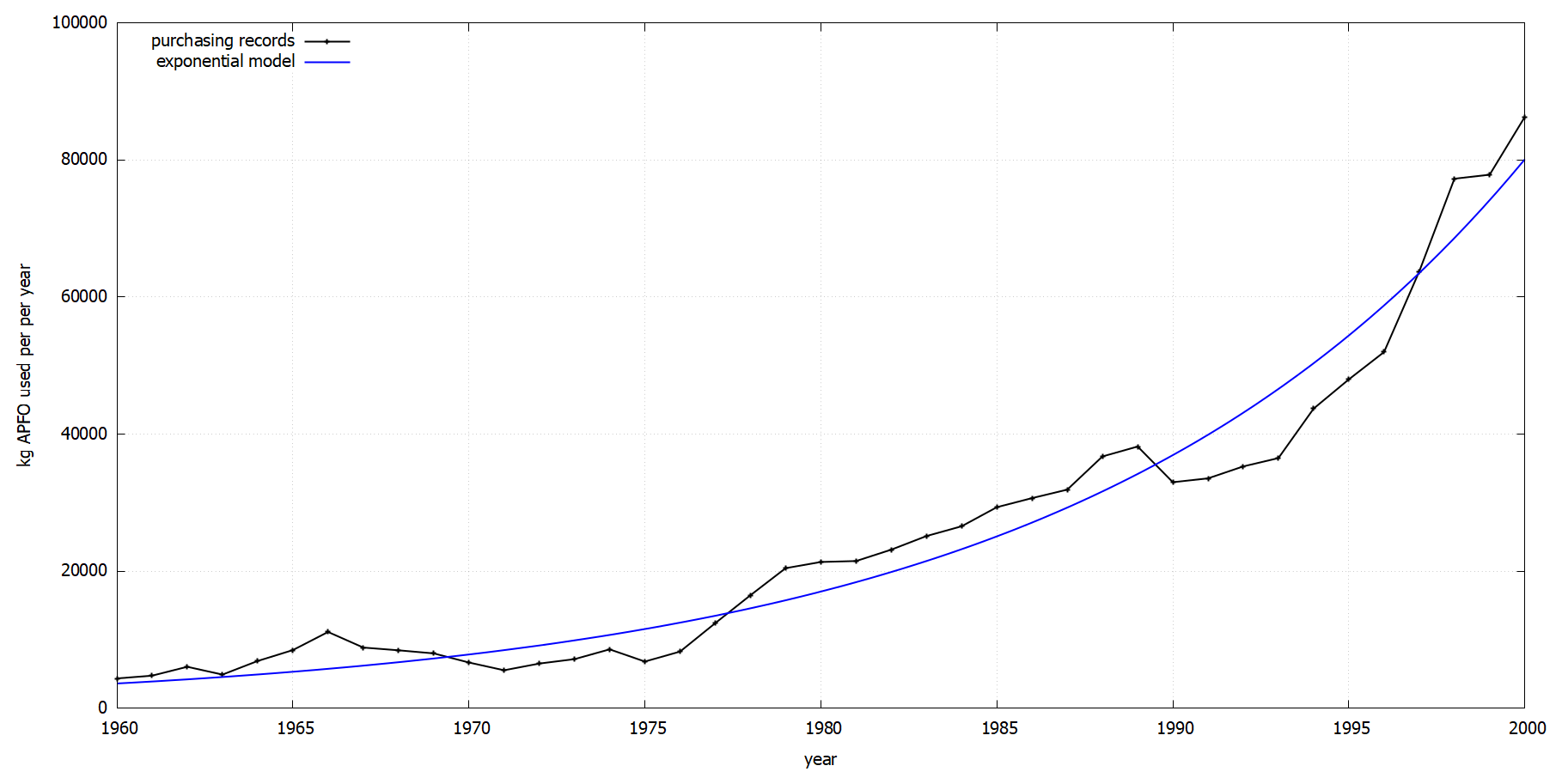
Figure 1 Total amount of APFO used in fluoropolymer production at the Dupont Parkersburg plant from 1951 to 2001 based on purchasing records. Adapted from Paustenbach et al. (2007a). The blue curve represents the exponential approximation used by POPE for fluoropolymer production plants in country group I.

Observable in the timeseries of used APFO in Parkersburg is the exponential increase up to the year 2000. As there is no known change in APFO usage rates this increase is attributed fully to an increase in production volume. An exponential fit to this part of the curve yields a yearly growth factor of 0.074 with R²=0.96.

Based on this example it can be assumed that without regulation or fade out an exponential increase in fluoropolymer production volume is reasonable.

Consequently, an exponential fit of the yearly fluoropolymer production volume is used for the remaining 25 production sites. For 11 of these, several years with approximated production volumes were available so that individual growth factors could be calculated. For the remaining 14 production sites only the production volume of one year is known. In these cases the average growth factor of plants where more data is available within the region was averaged and applied. These growth factors can be found in Table 4. The corresponding fits are available in the uploaded data (https://doi.org/10.5281/zenodo.12783504, Simon, 2024).

Table 4 Fluoropolymer production growth factors obtained through exponential regression for known production quantities in each country applied over the complete timespan.

For all fluoropolymer production sites, the opening and closing of factories is considered, specifically closings due to country specific regulations and bans. The production volume before the opening of a factory and after closure is set to zero accordingly. This is a simplification as after closure of a production site significant residual emission is expected, but already accounted for beforehand. Depending on the used transport model and circumstances, a retardation of emissions may be needed.

This allows to obtain an approximate production volume V for all included sites over the covered timespan to calculate the emissions according to Eq. (8).

As a second source of temporal change, the loss fraction according to Eq. (1) is included. The changes in loss fraction were subject of the study of Wang et al. (2014a). The authors differentiated between five periods with estimated loss fractions to water and air. Since the main concerns for these shifts were of economical nature, as for the early shifts the worrying effects on the environment were not yet known, it was assumed that country specific regulations played a minor role. Therefore no country specific scaling was performed here. The loss fractions were smoothed out over 10 years each to represent the expected gradual transition due to the adaptation of new technology. The temporal development of the loss fraction is depicted in Fig. 2

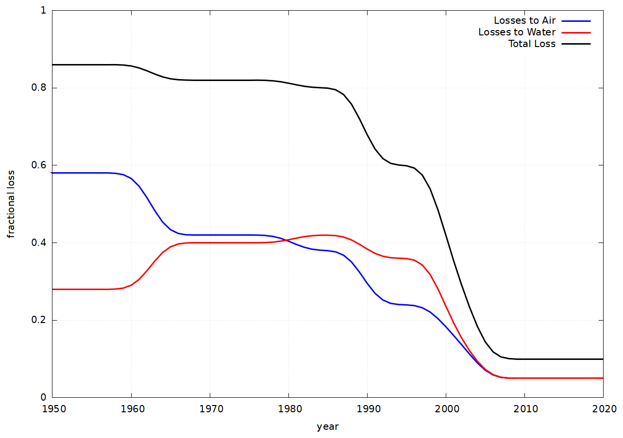
Figure 2 Loss fractions taken from Wang et al. (2014a) smoothed out over a 10 year period.

The emissions in a specific scenario s into medium m at time t $E_{s,m,t}$ are therefore approximated by

$$\begin{array}{}\text{(8)}& E_{s,m,t}=V_{\text{ref}}\cdot e^{k_s\cdot (t-t_{\text{ref}})}\cdot c_s\cdot f_{m,t},\end{array}$$

with the growth factor k depending on the scenario s, the reference production V_ref in the reference year t_ref the usage rate c_s, depending on the scenario and the loss fraction f_m,t at time t to the corresponding medium m.

2.6.2 Other Industries

Ohter industries than fluoropolymer production are handled methodically different in POPE. In this case loss fraction and usage rates are not applicable as neither the produced product quantities, nor the used PFAS mass per product volume are known. The temporal dynamics of emissions is therefore solely determined by the total estimated production volume of a site, assessed according to Sect. 2.4.2. The lower bound scenario assumes only linear growth forward in time from the corresponding reference period, as well as exponential growth backwards in time. The upper bound assumes exponential growth forward in time as well as linear growth backwards in time. The prescribed sector total is conserved in both cases.

Note that regarding the location of industrial sites no temporal change has been applied. The corresponding datasets (US EPA FRS, E-PRTR, and Nace Rev.2) are only available for recent years. It is therefore assumed that outside of fluoropolymer production no spatial shift of emissions over time apart from varying production growth rates and different regulatory impact takes place.

2.6.3 Product Use and Disposal

POPE assesses the temporal change in emissions due to product use and product disposal together. It is assumed that the emissions of waste water treatment plants and disposal sites follow the temporal trends of the related product emissions. This implies an included implicit time-lag. As disposed products are expected to slowly leach PFAS, depending on the product and environmental condition, the actual time-lag may be much larger than modeled by POPE. As this is hard to accurately assess, due to the limited data and wide range of products, POPE factors this time-lag into the upper and lower bounds.

The emissions of PFAS related products are changing over time via two different factors. On the one hand shift occurs implicitly with changes of population and GDP via their respective datasets. On the other hand, explicit scaling over time has to be applied to represent the growth in use of PFAS related products. Both factors will be explained subsequently.

As shown in the dataset by Chambers (2020) the population mostly follows exponential growth, although the growth factors are varying and are generally lower in country group I, and higher in country group II and III. Although the World's population approximately tripled from 1950 to 2020, the population in country group I grew on average about 50 %. Regarding the GDP, Kummu et al. (2018) provided data from 1990 to 2015. The GDP before and after this time period is extrapolated assuming exponential growth, using the average annual growth over the provided period as annual growth factor. This results in a global real GDP growth which is approximately five fold, with the same distributional trends as the population. The PFAS emissions grow implicitly with population and GDP.

With technological advancement, PFAS containing products grow more prevalent as a share of all consumer expenses. As an approximation, it is assumed that the use of these products grows proportionally with the industrial production volumes. Even though not all industrial production is exclusively for the consumer market, this is a proxy for the prevalence of PFAS containing products and forces zero product related emissions, before their first production.

The estimated production volume of PFOA and PFOS in the year 2009, when the study by Pistocchi and Loos (2009) was performed, serves as a benchmark production for these compounds. The product use and disposal emissions of a year are scaled by the fraction that the corresponding year's production volume represents of the benchmark production volume. This also implicitly accounts for a part of the emission time lag. This scaling is performed crosswise for the higher and lower bounds of the production volume and the emission per person, respectively.

One additional influence that POPE considers is the conflation of both factors, as for example production increases because there is more economic power demanding PFAS containing products.

This conflation is considered for the upper and lower bounds. Since the majority of the data set is extrapolated into the past, the conflation leads to an underestimation of the total global emissions. Therefore, two different approaches have to be taken for the upper and lower bounds, differing for extrapolation forward in time or backwards in time. Backwards in time the lower bound estimate assumes minimal overlap and neglects this effect, while the higher bound estimate eliminates the scaling with GDP and population by normalizing with the global population and GDP of the current year. This means, that the total emissions grow parallel to the corresponding industrial production volume. Changes in GDP and Population on the other hand redistribute the total emissions, depending if the region underperforms or overperforms compared to the global average growth of population and GDP. As the growth with total production volume far outpaces population and GDP growth, this rarely leads to a decline in local product related emissions over time, but the effect still has to be noted. While extrapolating forwards in time these different approaches for lower bound and higher bound estimate invert, now ignoring the overlap in the higher bound estimate and overcompensating by scaling with the global real GDP and population in the lower bound.

2.6.4 Aqueous Film Forming Foams

POPE considers two factors for the temporal development of AFFF emissions: increasing prevalence of PFAS as well as supra-national regulations and fadeouts. The latter are handled by country group and comprise regional total bans. The effects of upper limits for PFAS content of firefighting foams and changes in frequency of mandatory firefighting exercises are neglected.

To capture the gradual implementation, increased air travel volumes, as well as the increasing air travel security standards developing over the years, a linear approximation is used from the start date to the previously approximated yearly emission values for the corresponding year. Further than that, there was not sufficient data available to substantiate a modelled decline or increase in use or PFAS-content of firefighting foams and both were therefore set constant. Note that also no opening or closing of airports is implemented, as the expected influence is expected to be minor, especially since even closed airports may still act as significant pollution sources (Linderoth et al., 2016).

3 POPE Emission Inventory

The result of the introduced assumptions and methods applied in the POPE emission model is the POPE emission inventory (available for download at https:// permalink.aeris-data.fr/POPE), which contains global PFAS emission information for 5 different sectors, on a 0.5° equirectangular global grid, with a temporal resolution of one year, covering the years 1950 to 2020. Besides emissions into the atmosphere, the POPE emission inventory also contains emissions to rivers and the ocean by river-run off estimates.

The following sections explore the POPE emission inventory in detail. The results start with a general evaluation of the quality of POPE by comparing modelled river emissions with independent river measurements. This is followed by a comparison of global totals with the emission inventories by Prevedouros et al. (2006) and Wang et al. (2014a). Finally, the spatial distribution is examined in further detail by showing the aggregated land emissions and the direct emissions to oceans, before the temporal development of the global and regional totals are shown.

3.1 Global Totals

As POPE combines the emission inventories by Prevedouros et al. (2006) and Wang et al. (2014a) with other sources and socio-economic data, POPE is compared to these inventories to check its consistency with the original data. Figure 3 depicts this comparison for PFOA.

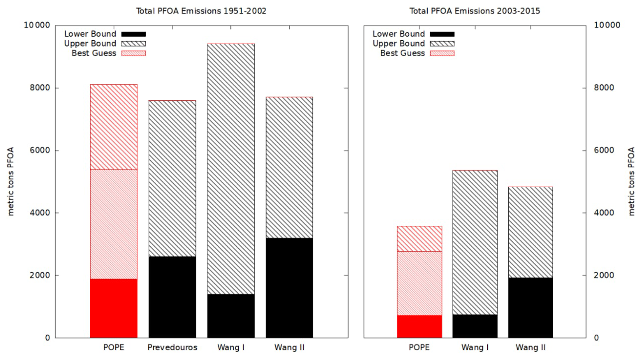
Figure 3 Comparison of total PFOA emissions for the upper bound, lower bound, and best guess of POPE for the time frames 1951–2002 and 2003–2015 to the emission estimnates provided in Prevedouros et al. (2006) and Wang et al. (2014a). The red bar indicates the model.

Figure 3 shows that between 1951 and 2002 the deviation of PFOA emissions in POPE relative to the other inventories is similar to the deviation of the chosen inventories relative to each other. The best guess scenario is compatible to all other estimates. This also holds true for the time period between 2003 and 2015. The upper limit of POPE is significantly lower than both upper limits of Wang et al. (2014b). This may be attributed to the partial exclusion of secondary emissions by precursors and other indirect sources (Wang et al., 2014b) to reintroduce them with a different methodology, which produces lower estimates. With the fade-out of PFOA and the simultaneous switch to other PFAS, precursors gain in significance in recent years (Wang et al., 2017a).

A similar picture is seen when comparing all PFCAs against the inventory of Wang et al. (2014a) as in Fig. 4.

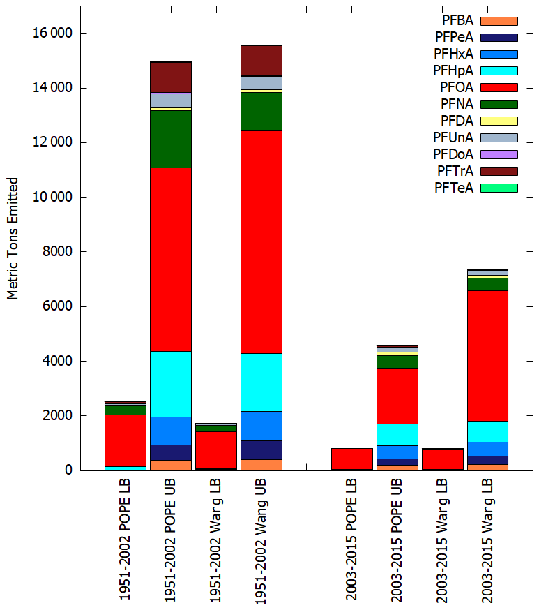
Figure 4 Comparison of the sum of all emissions of POPE for all PFCAs for the time frames 1951–2002 and 2003–2015 (Wang et al., 2014a).

POPE relies for the biggest emission sector: fluoropolymer production, on the inventory (Wang et al., 2014a). Therefore both are expected to yield similar results. Differences concern mostly the emissions in product use and disposal, airport firefighting and precursors. Even with these different approaches and the inclusion of additional data and redistribution in space and time POPE is in general agreement with Wang et al. Essentially, also the relative contribution of each individual PFCA is very similar. Biggest outliers are an underestimation of PFOA as stated before, as well as a slight overestimation of PFNA. One explanation for the overestimation of PFNA is the inverse effect observable for PFOA in recent years, as PFNA is generally more prevalent in Europe and the United States compared to Asia (Langenbach et al., 2021). As the bias in the emission estimates for country group I is positive, while it is negative for the country group II this distribution leads to an overestimation in total. As POPE does not take into account more emission sources per se and uses identical numbers for fluoropolymer production this is mainly related to the estimates regarding the emissions during product use and disposal, which Wang et al. (2014a) accounts for differently.

3.2 Spatial Distribution

This section presents the global gridded PFAS emissions over land as well as the expected river loads of PFOA to the global oceans.

Figure 5 depicts the aggregated total emissions in the best guess scenario for the time-period 1950–2020 for each grid cell for PFOA, PFOS, 8 : 2-FTOH and HFPO-DA representative of PFCAs, PFSAs, FTOHs and substitutions respectively.

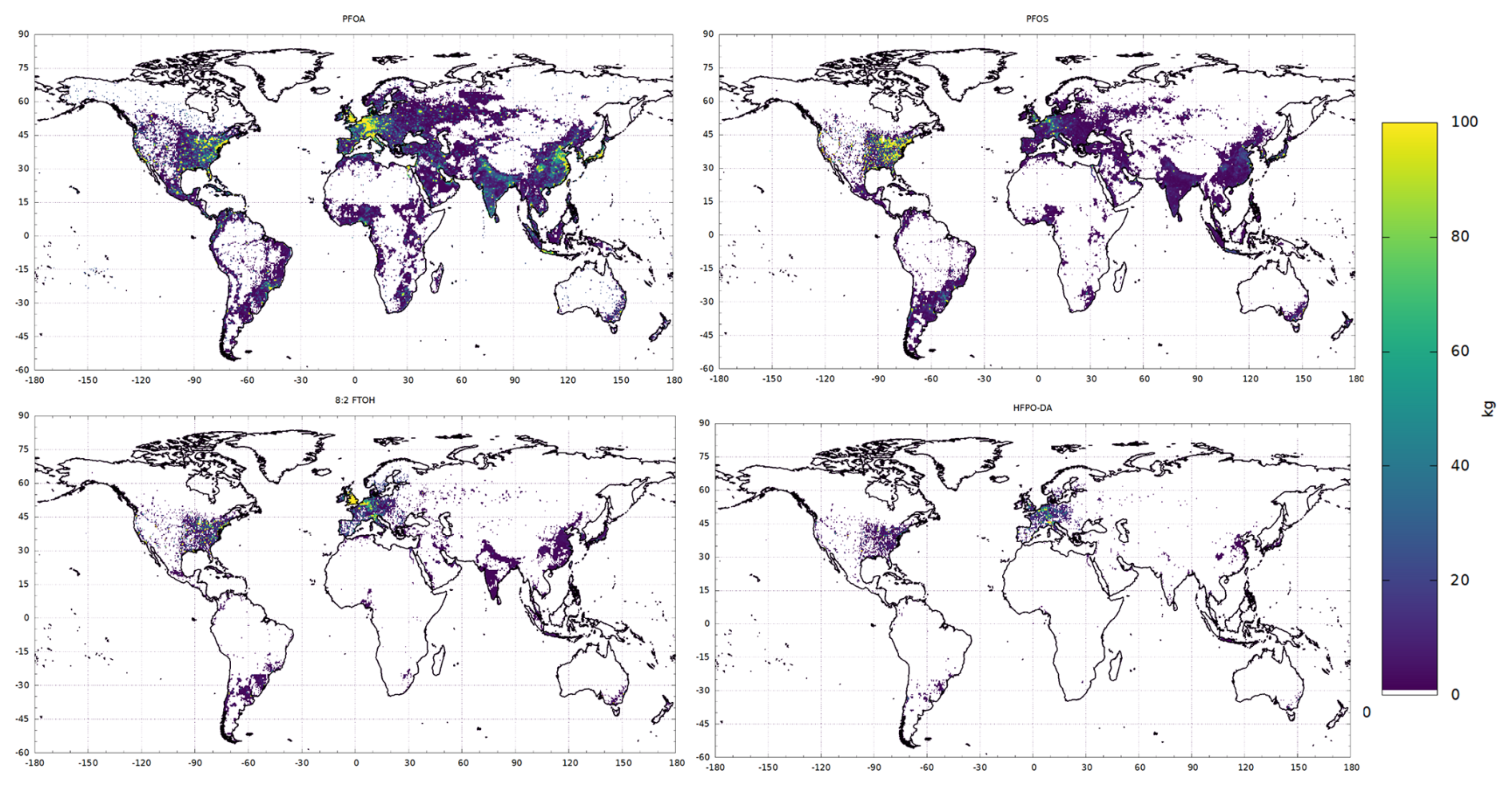
Figure 5 Global distribution of time-aggregated PFOA, PFOS, 8 : 2-FTOH and HFPO-DA emissions per grid cell during 1950–2020. The grid resolution is 0.5° × 0.5°. The upper cut-off value is 100 kg, the lower cut off value is 1 kg.

Figure 5 reveals the direct influence of population density on PFOA and points out the main regions producing and using PFOA. These are central Europe, the east coast of the USA, Japan and the east coast of China. South and Central America, Africa and Oceania play a negligible role for the total emissions of PFOA. This map reflects the general expected distribution by GDP and population, whereas fluoropolymer production sites with significantly higher total aggregated emissions are in this case close to population centers. The importance of certain regions in relation to others changed over time, which will be discussed in Sect. 3.3.

The emissions of PFOS are typically associated stronger with diffuse sources such as airport firefighting (Glüge et al., 2020). This is visible in Fig. 5 on a global scale, occuring widely with less hotspots. Also shown is the disparity of usage between the United States and other regions of the world. Within the US, again the east coast shows much higher emissions than the west coast.

As a replacement compound the total HFPO-DA emissions are in absolute numbers lower than legacy compounds up to now. It is mainly used in regions where PFOA has been phased out such as Europe, Japan, and the United States. This is reflected in the total aggregated emissions. Although the limited data suggest an incomplete picture, HFPO-DA emissions are more regionally contained than other PFAS. The production emissions dominate over the emissions over product lifecycles due to its novelty. The high availability for transport based on its physico-chemical properties may still lead to high concentrations distant to source regions.

8 : 2 FTOH is the most prevalent precoursor for PFOA. The distribution of the total aggregated emissions shown in Fig. 5 show the prevalent usage in Europe with comparatively high emission loads the United Kingdom. These are mainly related to the usage of 8 : 2-FTOH in advanced apparel manufacturing and treatment of surfaces. This emission distribution suggests that significant PFOA emissions can still be expected by precoursers alone.despite the upcoming total fade-out in the European Union.

3.3 Temporal Development

As PFAS were only produced in modern times and do not occur naturally, any emission inventory covering the industrial scale production in the years from 1950 onwards are, for the most part, temporally complete. Emissions before the industrial scale production are assumed to fall below the model uncertainty. Over the majority of this time span the dynamic is characterized by an increase in emissions.

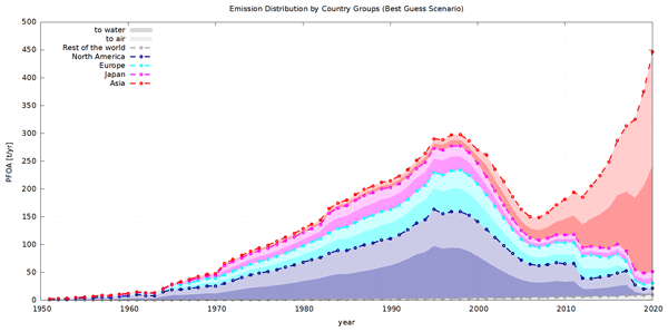
But the relative importance of the individual regions was not the same over time. Important for the emission dynamics of legacy PFAS is the spatial shift of production from country group I to country group II after the year 2000. To illustrate how this dynamic is represented in POPE, Fig. 6 shows the yearly emission of the best guess scenario for 5 geographical regions.

Figure 6 Total PFOA emissions by country group in the best guess scenario.

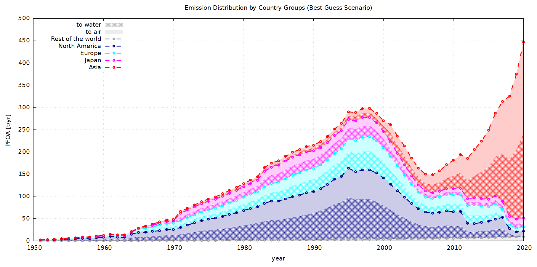
The major reduction of PFAS emissions in the United States and worldwide after 2000 is associated with multiple studies regarding the health risks of PFOA. These concerned the Dupont plant in Parkersburg, West Virginia, which up to this point was the largest emitter of PFAS in North America. The region with the second largest emission of PFAS during this time was Europe, however, the production and usage of products containing PFAS started significantly later. Japan behaved differently than the rest of Asia, as it largely followed the trends of the United States and Europe, also showing a slow fade-out after 2000. During this time it is clearly visible that the global production of fluoropolymers shifted mainly to China. Additionally, the general increase of living standards in Asia reflected also in increased use and disposal of PFAS-related products.

4 Evaluation of the Emissions to Water

An advantage of the POPE emission inventory is the capability to model the release of PFAS into rivers and oceans consistently with the emissions to air. These riverine emissions were used to evaluate the POPE emission inventory. To calculate the PFAS river runoff into the oceans, the hydrological discharge (HD) model of Hagemann et al. (2020) was used and compared to available concentration measurements in rivers.

4.1 Riverine Transport Model

The HD model calculates the lateral transport of water over the land surface to simulate discharge into the oceans. After its initial development (Hagemann and Dümenil, 1998), it has been validated and applied in many studies (Hagemann and Dümenil Gates, 2001; Hagemann et al., 2020; Hagemann and Stacke, 2022). The HD model requires gridded fields of surface and subsurface runoff as input with a temporal resolution of one day or higher. Similar to the experimental setup described in Hagemann and Stacke (2022), these were generated by the HydroPy global hydrology model. As meteorological forcing, Global Soil Wetness Project Phase 3 forcing data (Dirmeyer et al., 2006) were used from 1950–1978 and the WATCH Forcing Data based on ERA5 re-analysis (Cucchi et al., 2020) from 1979–2019. The HD model incorporates a framework for the transport of substances at the speed of the river flow. The calculated riverine emissions included in the POPE emission inventory were used as a direct input into the river, following the upper, lower and best guess estimates respectively. The emission volume was assumed to be constant over the year and homogeneous over any given gridcell. No chemical or physical transformation within the river is conducted as it is expected to play a minor role for river concentrations (Xu et al., 2021).

4.2 River Concentrations

The calculated concentrations according to the POPE emission inventory and HD model are compared to several concentration measurements regarding the bias, trend along the river and to what extend the estimated bounds act as such. To quantify the relationship between the concentration measurement and the calculated bound according to POPE, the modified Root Mean Squared Normalized Error (RMSNE) is calculated for each study and each river individually according to

$$\begin{array}{}\text{(9)}& \text{RMSNE}=\sqrt{{\displaystyle \frac{\mathrm{1}}{n}}\sum _i({\displaystyle \frac{c_{\mathrm{l},i}+\frac{\mathrm{1}}{\mathrm{2}}{\mathrm{\Delta }}_i-c_{m,i}}{\frac{\mathrm{1}}{\mathrm{2}}{\mathrm{\Delta }}_i}}{)}^{\mathrm{2}}}.\end{array}$$

Here, c_m,i is the concentration of the ith measurement, c_l,i the simulated concentration in the lower bound scenario at the position of the ith measurement, n the number of measurements taken for that river in the corresponding study, and Δ_i the difference between the upper and lower bound scenario at the position of the ith measurement. According to this metric, values below 1 indicate that all observed values fall in between the model bounds, while a value of RMSNE = k signifies that the average difference between bound and measurement is $\frac{k^{\mathrm{2}}-\mathrm{1}}{\mathrm{2}}$ times as large as the difference between upper and lower bound.

4.2.1 Trends along Rivers

Figure 7 shows PFOA concentrations in a selection of rivers including rivers close to former and current fluropolymer-production sites, to capture trends along part of the river's length. Pictured are six rivers, with two of them in the United States, Europe and China, respectively. These are the Rhine (Heydebreck et al., 2015) in the year 2013, the Elbe (Heydebreck et al., 2015) in the year 2014, the Cape Fear River (Sun et al., 2016) in 2013, the Ohio River (Galloway et al., 2020) in the year 2016, the Yangtze (Jin et al., 2009) in 2003 and the Xiaoquing in 2014 (Heydebreck et al., 2015). The rightmost values of each individual river are closest to the sea. Note, that the distance between two measurements may be less than the resolution of the emission-model and therefore, for both the same upper and lower bound may apply. Also note, that the measurements by Sun et al. (2016) were mostly under the quantification limit, whereas the measurements of the Xiaoqing by Heydebreck et al. (2015) yielded much higher concentrations than the calibration range, leading to potentially higher uncertainty.

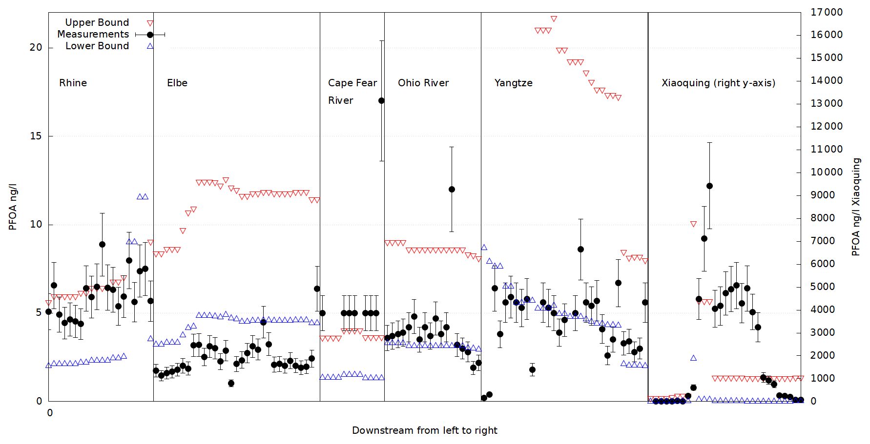
Figure 7 Overview of several river concentration measurements by Sun et al. (2016), Pétré et al. (2022), Heydebreck et al. (2015) and Jin et al. (2009) in comparison with the upper and lower bound estimation by POPE. The rightmost values are closest to the sea.

POPE and the measurements show similar trends over the considered length of the rivers. Deviations seem to be mostly in form of a consistent bias over the whole river length for all rivers. The expected changes due to an increase in emission load relative to the total watermass follow the expectation. This is very much visible for the Rhine, Elbe, Ohio River and Yangtze. Individual extreme values as for example directly at the plant in the Ohio River, or specific high points at the Elbe or Cape-Fear River are smoothed out due to the nature of the model. Differences in the trend seem comparatively lower to the overall bias. This may suggests large scale distributional errors, affecting the attribution of emissions to whole regions or sectors rather than large local fluctuations due to inaccurately placed point sources or wrong attribution of production volume.

Large relative and the largest absolute deviation for the Xiaoquing River suggest that the modelled emissions in its watershed are underestimated in the POPE emission inventory. In the regions of highest concentration near the plant, the upper bound falls short by an order of magnitude. Downstream the concentration in the model falls to a much lower level than the measurements suggest. One possible explanation may be the influence of atmospheric deposition of emissions to air, which increase the river concentration as a whole and may exend the influence of the production plant downstream. Other explanations may be due to the small length of the river, production variation influencing the single measurement day, or an underestimation of the total emissions in Asia or country group II respectively. Relative overestimation as with the Yangtze river on the other hand suggest again rather distributional errors. Based on the distribution method in China this may hint to the fact, that the relative impact of population as emittent, combined with population and GDP as a proxy underestimates the impact of few high emission point sources. Furthermore, this can be impacted by the assumption that the use of recovery methods during the production process is on the same level as reported for e.g. the United States. This assumption was made due to a supposed strong economic motivation in reusing processing aids. Assuming loss fractions as reported for the United States in the 1950s and 1960s as in Fig. 2 could increase PTFE-production emissions by a factor of about 10 and therefore explain part of the missing emissions and deviation from observations.

4.2.2 Average Error and Bias

Shown in Table 5 are the RMSNE and the mean difference between measured concentration and the modelled concentration for the best guess estimate. Additionally shown are the Pearson correlation coefficients r to assess how well the model captures the trend along the river, for all rivers where multiple measuring points are available.

Sun et al. (2016)Pétré et al. (2022)Pétré et al. (2022)Pétré et al. (2022)Mclachlan et al. (2007)Liška et al. (2015)Mclachlan et al. (2007)Mclachlan et al. (2007)Heydebreck et al. (2015)Mclachlan et al. (2007)Heydebreck et al. (2015)Pétré et al. (2022)Pétré et al. (2022)Mclachlan et al. (2007)Mclachlan et al. (2007)Mclachlan et al. (2007)Galloway et al. (2020)Mclachlan et al. (2007)Mclachlan et al. (2007)Michigan Department of Environmental Quality Water Resources Division (2019)Heydebreck et al. (2015)Mclachlan et al. (2007)Mclachlan et al. (2007)Mclachlan et al. (2007)Mclachlan et al. (2007)Mclachlan et al. (2007)Heydebreck et al. (2015)Heydebreck et al. (2015)Jin et al. (2009)

Table 5 The modified Root Mean Squared Normalized Error (RMSNE), correlation coefficient r and the bias between measurements and simulated values in comparison to several studies.

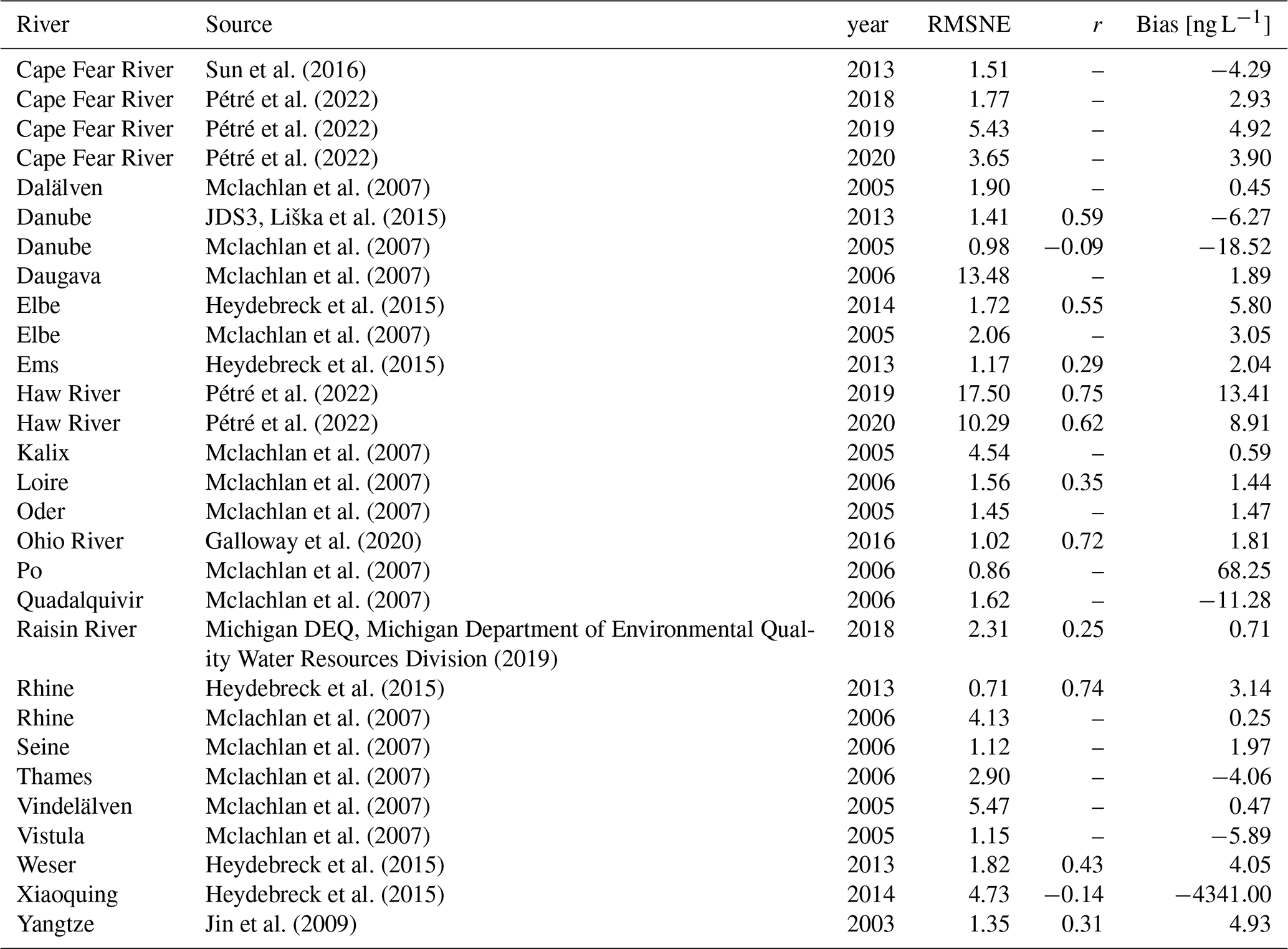
The results show varied picture. This is attributed to a multitude of factors, which may be related to the emission inventory but also due to the comparison of a snapshot in time that the river measurements provide to averaged model results, or processes in the river not accounted for, intra-annual variations in production emissions as well as a general environmental retardation. This also becomes visible in the general better agreement for larger rivers for which the relative influence of these variations is smaller. Additionally, there is a better agreement for rivers which are well researched as the Rhine and the Ohio River.

The model tends to overestimate emissions to rivers without major production sites, with positive biases and RMNSEs significantly larger than one, as for example at the Haw River or Daugava. There, the emissions are mostly impacted by the smaller manufacturing industry point sources for which size data is not avaialable but may hint at smaller production volumes and emissions.

On the other hand, PFAS concentrations in rivers which are situated near industries which are not included in the model may deviate significantly. This is for example visible for the Danube, similar to the results of Lindim et al. (2015a). This is exacerbated by the broad approach of industry sectors where corresponding sectors with high average PFAS emissions like apparel manufacturing may in reality be dominated by a few sites with relevant production of e.g. outdoor apparel, while most sites emit little to no PFAS at all (Glüge et al., 2020).

The correlation coefficients r of the measured concentrations to the POPE best guess emission estimates measures the agreement in dilution and emission input for both. These are mostly positive in the range of r=0.25 to 0.75. Most of the correlation coefficients show, that the general trend of increasing concentration with increasing emission sources and decreasing concentration with increasing runoff is captured. The lowest value of −0.14 is for the Xiaoquing River. Here not only the absolute value is not captured, but also the trend reverts. This may suggest differing positions of the actual emission input and the modelled input.

The calculated biases are mostly in the order of magnitude of the observed concentrations. They hint at a distribution problem with an underestimation of Chinese single point sources and an overestimation of European and North-American emissions. As POPE is neglecting emission sources, as for example several possible precursors, and showed lower estimates for diffuse emissions than previous emission estimations a negative bias would have been expected. This may mean, that other factors such as loss fractions or the used average emission per person are too high. A fraction of the emissions may also be wrongly distributed, for example from country group II to country group I, which is mainly based on population and GDP Asia might be wrongly attributed to Europe and the USA. Factors like a bias in certain input data, as for example the per person emission, might also cause this trend.

4.2.3 Total loads

For most environmental concerns the sum of PFAS is the relevant quantity. Figure 8 shows how the sum of PFAS in POPE, transported with the HD Modell, relates to the measured sum of PFAS in the studies from Table 5.

The shown ranges are spatio-temporal ranges covering all measurements over the whole river length. All model data relates to the best guess scenario and the range over all corresponding gridcells with the median indicated by the black bar.

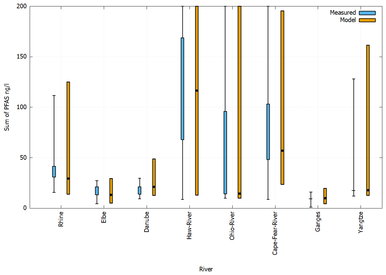
Figure 8 Comparison of the range of the sum of all measured PFAS in selected rivers with the best guess estimate of POPE. The whisker-bars indicate the measured quartiles, where available. The upper quartile of the Haw-Ohio and Cape-Fear-River reach 256, 231 and 204 ng L⁻¹ respectively. The black line in the modelled results indicates the median concentration of all corresponding gridcells.

There is high overlap between the measured ranges and the ranges based on the POPE emission inventory. As the correlation factors indicate measured and calculated values do not always agree in space and time. The high temporal variation of the river loads is not well represented in the model. The shown bias is not identical for all rivers. Concentrations in heavily industrialised river basins are underestimated while concentrations in basins with less industry are overestimated. The general concentration range is captured adequately, although the coarse resolution of POPE tends to smooth local high emissions. At the same time the used gridcell mask is in total bigger than the corresponding rivers leading to the inclusion of a wider range of values. Adding all substances improves the agreement suggesting non-systematic errors canceling each other out. which is why the relative contribution of individual PFAS will be assessed later.

4.2.4 Relative Contributions to the Total

Apart from the total concentration in any given river it is of interest to compare the relative PFAS fractions of the POPE emission inventory with concentrations measurements in rivers. Figure 9 shows this fraction of the total PFAS load averaged over all measurements, or the corresponding gridcells respectively. These fractions consider only substances found in both POPE and the study at hand meaning the shown substances do not necessarily represent the most important contributors to the total PFAS load in each river.

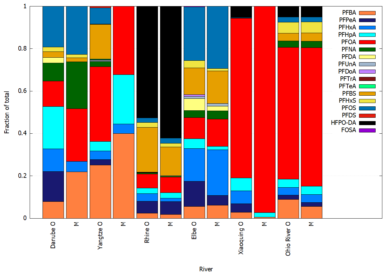
Figure 9 Relative fraction of all PFAS considered by POPE and the respective studies for a selection of rivers in the sections with measurements available. O indicates an observation, M designates the corresponding modeled result. The order of substances in the legends corresponds to the inverse vertical order of fractions.

The best agreement is again found for the most extensively studied rivers, the Ohio River and the Rhine and the most extensively studied PFAS of PFOA and PFOS. The Rhine is especially of interest as it is influenced heavily by the replacement of PFOA by HFPO-DA. Even though the absolute PFAS concentrations in the Rhine tend to exceed the upper bound the fraction of HFPO-DA and therefore the replacement factor used in POPE is compatible with the measurements. The relative fraction of PFBA on the other hand may hint at a distribution error between countries. The Danube and Yangtze show large differences especially for PFBA and PFNA. The latter was already observable in the totals and is most likely associated with an inaccurate split between the two associated Fluoropolymers PTFE and PVDF. Similar distributional deviations as for PFBA can also be observed for PFHpA which is assumed to be dominantly used in Asia while measurements show an unknown source near the Danube. The two chinese Rivers Yangtze and Xiaoquing suffer again from the insufficient data on used PFAS mainly due to the simplification that country group II uses mostly legacy PFAS while the measurements show that the usage is broader than anticipated. Additionally, some unknown industries not associated with PFSA usage in POPE seem to have a big influence on the Yangtze basin, which is not considered in POPE.

These gaps pose opportunities for improvement of POPE with more accurate industrial data in country group II.

4.3 Ocean Emissions

Many relevant PFAS are acids or alcohols, some with very low acid dissociation constants (Buck et al., 2011) like PFOA, they are expected to remain dissolved, once they were in contact with water masses, cloud droplets or water soluble aerosol particles.

Therefore the global oceans are highly relevant for the long term fate of PFAS. Table 6 lists the total calculated PFAS load by rivers over the time-period 1951 to 2020 to the Arctic Ocean (AO), North Atlantic (NA), South Atlantic (SA), North Pacific (NP), South Pacific (SP), Indian Ocean (IO), Mediterranean Sea (MS), North- and Baltic Sea (NBS) in the upper bound scenario, as simulated by the HD model based on POPE emissions. Figure 10 depicts the river discharges of PFOA into the Arctic Ocean, the North Atlantic Ocean, the South Atlantic Ocean, the North Pacific Ocean, the South Pacific Ocean, the Indian Ocean, the Mediterranean Sea and the North- and Baltic Sea over time for the upper bound scenario. Note that this only contains riverine emissions without any atmospheric transport and without exchange between oceans. This means, for example high levels of PFAS in the North Atlantic are expected to cause a high PFAS burden on the south Pacific and the Arctic ocean, due to interoceanic exchange. This reemphasizes the need for transport modelling to assess the long term fate of PFAS in the oceans and atmosphere.

Table 6 Total PFAS river load [t] for the time period 1950–2020 and relative fractions [%] released to the Arctic Ocean (AO), North Atlantic (NA), South Atlantic (SA), North Pacific (NP), South Pacific (SP), Indian Ocean (IO), Mediterranean Sea (MS), North- and Baltic Sea (NBS) in the upper bound scenario.

Figure 10 Total PFOA emissions to oceans in the upper bound scenario.

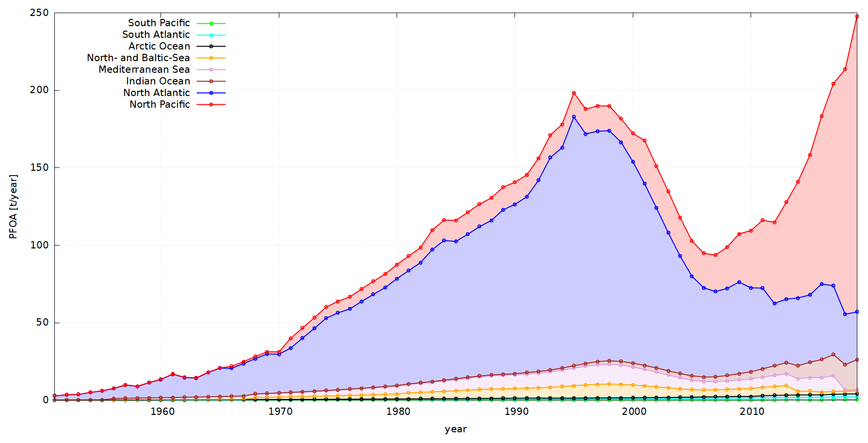
As shown in Table 6 again the northern hemisphere is far more affected by PFAS pollution than the southern hemisphere. The North Atlantic and North Pacific received the majority of PFAS loads. Based on Fig. 6 large east-west concentration gradients are expected in both seas. Even small marginal seas, like the Mediterranean Sea, are subject to significant pollution.

The pictured PFAS fluxes into the oceans in Fig. 10 mirror the general trend of the regions. However a significant flux of PFOA to the North Atlantic mainly by precursors and emitted through PFOA containing products persists. It becomes apparent, that the majority of the emissions from North America enter the North Atlantic rather than the North Pacific, while the distinction between the Mediterranean and the North- and Baltic Sea shows, that the significantly smaller contribution of Europe splits roughly equally between these two. The contributions of Europe to the North Atlantic PFOA concentrations via the direct river runoff is minor and comes only into play in exchange with the north sea. Over the whole time period, the Arctic Ocean and the southern Oceans are only slightly affected by direct river discharges. The concentration levels found for example by Joerss (2020) or Boitsov et al. (2024) may therefore be closer related to atmospheric transport and the exchange with neighboring oceans.

5 Code and data availability

The code and data of the POPE Emission model is available at Zenodo (https://doi.org/10.5281/zenodo.12783504, Simon, 2024) distributed under Creative Commons 4.0 Attribution. Alternatively the POPE emission inventory is also publicly available in GEIA's (Global Emission InitiAtive) ECCAD data portal: (https://permalink.aeris-data.fr/POPE, last access: 3 June 2025).

6 Discussion and Outlook

The PFAS emission model and inventory POPE builds on existing global inventories by disaggregating decadal total emission loads with socioeconimc proxies and industrial data. POPE collects several local and regional emission estimations to build one consistent scenario capable dataset, distinguishing between 5 different sectors and two compartments in a 0.5° resolution gridded model ready format. Upper and lower bounds as well as a best guess estimate are provided. POPE extra- and interpolates existing production volumes and couples use and disposal emissions to these production estimates to obtain an annual complete inventory from 1950 to 2020. POPE extends methods used for emission estimations of legacy PFAS to precursors and novel PFAS to get one step closer to a complete picture of PFAS emission. The consistent method is easily expandable to cover more PFAS as soon as the necessary data is available.

The POPE emission inventory is compatible with emission inventories it builds upon but expects mostly slightly lower emissions based on its different approach to use and disposal of PFAS products. As depicted in in Fig. 6 and Table 6 (Sect. 3.3) POPE is able to capture the main dynamics concerning the spatial and temporal trends in PFAS emissions:

• North America and to a lesser extent Europe and Japan dominate the PFAS emissions in the twentieth century.

• A temporal shift of emissions from Europe and North America to Asia starts after the year 2000.

• Significant emissions remains even after the total or partial fade-out of legacy PFAS such as PFOA and PFOS.

Different application profiles as well as national differences in the prevalence of different PFAS are captured by the POPE emission inventory.

Legacy PFAS can be exemplary to estimate emissions for precursors and novel compounds PFAS.

POPE has been evaluated with independent data based on PFAS concentrations in major rivers (Sect. 4). Although the emissions to water paint an incomplete picture and the comparison of averaged model results with concentration measurements has limited informative value, these results hint towards the possible usefulness of the POPE emission inventory. As expected, the best agreement regarding concentration measurements was found for Europe and the United States, as the model relies heavily on data from these regions (See Table 5 and Fig. 7). Found biases are inconsistent showing no trend of an total over- or underestimations. The trend along rivers indicates a successful source apportionment. Long time series in European rivers could help to evaluate the temporal quality of the emission inventory. In Asia, PFAS emissions seem to be generally underestimated, while some species found in rivers cannot be attributed to a source at all. The POPE model as a whole could be improved by more data on the location, production volume and expected loss fractions of fluoropolymer production sites in Asia, as well as better profiles which PFAS are in use and in which industries. For the southern hemisphere, there is no independent data for evaluation available.

Deviations in the evaluation could most of the time be attributed to a too homogeneous distribution, limited either by the model resolution or the necessary reliance on proxies. A two tracked approach as taken for non fluoropolymer industries in Europe with locations and employee numbers is leads to a promising emission estimation. Bottom-up estimated emissions exhibit better agreement of measured concentration and modelled concentration as shown in Fig. 9.

For all purposes, the inclusion of more individual industrial sites with associated production volumes and loss fractions is needed. Studies similar to the ones already performed for PFOA and PFOS on major industrial sites and airports for emerging PFAS such as GenX and ADONA could help to represent their emissions more accurately. More consistent reporting of production volumes and in cases of shifts between compounds replacement factors are needed to obtain useful emission values for GenX and ADONA. FOSA also shows significant knowledge gaps regarding emissions considering its relative importance for the formation of PFOS.

The spatial and temporal trends exhibited in the POPE emission inventory reemphasize the relevance of numerical multi compartment transport modelling. With the growing importance of product related emissions and precursors it is clear that even with strict PFAS regulations in place, significant emissions will still occur over extended time periods. The expected concentration gradient between regions poses the question of the importance of long range atmospheric and marine transport to remote locations like the Arctic. The geographical shift in industrial production leads to competing influences of legacy emissions and imported emissions from other countries.

POPE can support advancing multi-compartment transport modeling with consistent global emission data for PFAS, distinguishing between emissions to rivers/oceans and emissions to the atmosphere. This enables models to identify source-receptor relationships for PFAS pollution and to simulate different scenarios to predict its transport and concentration in multiple compartments. As the POPE emission inventory begins with the first industrial scale production of PFAS in 1950 chemistry transport models can be run independently of initial conditions. Furthermore, it is possible to perform simulations in non-equilibrium states, capturing the dynamics of increasing production, followed by a local fade-out and spatial shift of global PFAS emissions. The POPE framework is applicable to other PFAS not yet considered and will be extended as data becomes available.