Long-term solar-induced fluorescence data record from GOME-2A and GOME-2B (2007–2023) using the SIFTER v3 algorithm

Design differences in sensors and retrieval algorithms complicate the harmonisation of space-based solar-induced fluorescence (SIF) observations. The GOME-2 series, with its identical sensor design, offers potential for constructing a long-term coherent record. However, instrumental artefacts, such as degradation, affect the sensors differently and diverge the intersensor SIF observations. Achieving internal consistency within each record is therefore a critical first step in harmonisation. We present a combined GOME-2 SIF dataset for 2007–2023 that consists of GOME-2A (January 2007–December 2017) and GOME-2B SIF (July 2013–December 2023) data. Both individual records are retrieved using the previously developed SIFTER v3 algorithm, which applies time-, wavelength-, and scan-angle-dependent degradation corrections. Spatial agreement between GOME-2A and GOME-2B SIF during the overlapping period was strong (r≥ 0.96), although viewing geometry differences caused substantial systematic biases, specifically over high activity regions; these were reduced to within 2 % by constraining to common viewing zenith angle ranges. In terms of temporal alignment, most analysed regions showed no significant step change at the July 2013 sensor transition, from full-swath GOME-2A to GOME-2B SIF. Small offsets in Eastern China and the Amazon were corrected for using a simple additive correction, which improved the coherence and agreement with independent GPP estimations from FluxSat. Finally, the GOME-2 records align closely with FluxSat GPP and TROPOMI SIF across various biomes, and support monitoring of vegetation activity over 17 years. Our work presents a framework for detecting and, when necessary, correcting intersensor offset biases, enabling the use of GOME-2A and GOME-2B SIF as a single record. Moreover, it offers guidance for harmonising multi-sensor datasets and for other causes of potential structural breaks in long-term observation records. The GOME-2A and GOME-2B SIF (obtained in this study) datasets are available at https://doi.org/10.21944/gome2a-sifter-v3-solar-induced-fluorescence (Anema et al., 2025a) and https://doi.org/10.21944/gome2b-sifter-v3-solar-induced-fluorescence (Anema et al., 2025b), respectively.

1 Introduction

Terrestrial vegetation plays a crucial role in the carbon cycle, yet it also represents one of the largest uncertainties in future climate scenarios. Understanding changes in vegetation dynamics is essential for quantifying global carbon fluxes and sustaining food production. This highlights the need for long-term, global-scale vegetation monitoring. Satellite-based retrievals of solar-induced fluorescence (SIF) constitute a powerful tool to track vegetation dynamics at local to global scales. SIF observations are directly related to photosynthetic activity and, thus, carbon uptake (Mohammed et al., 2019). Previous studies have shown SIF to be sensitive to disturbances such as droughts, wildfire impact, and land-use change and to outperform traditional greenness indices like NDVI (e.g. Chen et al., 2021; Magney et al., 2019; Anema et al., 2024; Zhang et al., 2023; Gerlein-Safdi et al., 2020).

In recent years, advancements in SIF retrieval from spectrometer instruments have facilitated the growing number of SIF datasets obtained from various satellite missions, such as GOME, SCIAMACHY (Khosravi et al., 2015; Köhler et al., 2015), GOSAT, the GOME-2 series (Joiner et al., 2013; van Schaik et al., 2020; Anema et al., 2025a), TROPOMI (Köhler et al., 2018; Guanter et al., 2021), OCO-2 (Sun et al., 2018), OCO-3 (Doughty et al., 2022), and upcoming missions like FLEX (Vicent et al., 2016) and the CO2M series (Noël et al., 2024). These datasets have proven to be highly valuable for monitoring vegetation phenology and ecosystem productivity across various spatial and temporal scales (e.g., Turner et al., 2021; Wang et al., 2019; Zhang et al., 2022; Liu et al., 2021). However, the harmonisation of these datasets is challenging as merging is complicated by discrepancies in satellite characteristics and retrieval settings, such as local overpass time, observation geometry, spectral, spatial and temporal sampling, and the retrieval window spectral range (Parazoo et al., 2019; Sun et al., 2018).

Retrieving SIF from the GOME-2 instruments offers a unique opportunity to circumvent many of the intersensor discrepancies that limit harmonisation. Three instruments, launched in sequence as part of the Metop series, GOME-2A in 2006, GOME-2B in 2012, and GOME-2C in 2019, follow the same design and have consistent equatorial overpass times, all crossing at 09:30 a.m. The instrumental similarities minimise biases between sensors, offering potential to obtain a consistent long-term SIF record. Currently, GOME-2A provides the longest individual SIF record with continuous global coverage to date and has been widely used to investigate vegetation dynamics (Gerlein-Safdi et al., 2020; Chen et al., 2021; Fancourt et al., 2022). A robust merged GOME-2 record enhances our ability to study long-term vegetation dynamics, but would also serve as a valuable benchmark for harmonising SIF datasets, owing to its long duration and limited intersensor biases.

To our knowledge, no study has combined GOME-2 SIF into a long-term SIF record and assessed its coherence. A major challenge in obtaining a robust GOME-2 SIF record is its sensitivity to instrumental artefacts, particularly reflectance degradation, which can lead to false temporal trends in SIF (van Schaik et al., 2020; Zhang et al., 2018; Koren et al., 2018). If not adequately corrected for, these trends make the data unsuitable for long-term vegetation analysis (Parazoo et al., 2019), and hinder harmonisation across sensors (Wen et al., 2020; Wang et al., 2022). Our SIFTER v3 retrieval algorithm addresses this issue with an advanced degradation correction that is time, wavelength, and scan-angle dependent, following the reflectance degradation characteristics closely (Anema et al., 2025a). Other GOME-2 SIF products, such as TCSIF and LT_SIFc^* (Wang et al., 2022; Zou et al., 2024), also apply time-dependent corrections, but ignore wavelength and scan-angle dependencies of degradation. Notably, the scan-angle dependency was found to be of similar magnitude to the temporal component, making its omission a substantial source of bias (Anema et al., 2025a). Anema et al. (2025a) demonstrated the algorithm's effectiveness by obtaining a 2007–2017 GOME-2A SIF record with temporal stability, internal consistency, and strong correlation with independent data. Building on this work, we apply the same approach to retrieve GOME-2B SIF over mid-2013 to 2023 and evaluate its potential to use both datasets as a single coherent combined SIF record spanning from 2007 to 2023.

Our objectives are threefold. First, we retrieve GOME-2B SIF using the SIFTER v3 algorithm and level-1b Release-3 (R3) data to ensure consistency with the existing GOME-2A SIF record by Anema et al. (2025a). The degradation correction parameters are tailored to the specific reflectance degradation characteristics of GOME-2B. Second, we assess the spatial intersensor consistency during their overlapping tandem phase (from July 2013), using co-sampling methods to isolate sensor-specific biases. Third, we evaluate temporal coherence and demonstrate a framework to identify and, where necessary, correct intersensor offsets, enabling a coherent long-term combined GOME-2 SIF record. Six representative vegetated regions across diverse biomes are used as case studies to examine the intersensor agreement and GOME-2 SIF performance in capturing vegetation dynamics accurately. We present the GOME-2B SIF dataset, with measurement uncertainties, which can be combined with our previous GOME-2A SIF dataset into one GOME-2 SIF data record spanning from 2007 to 2023.

2 GOME-2 instruments

The GOME-2 instruments are part of the payload on the Metop satellite series, which consists of three identical satellites, Metop-A, Metop-B, and Metop-C, launched sequentially to enable long-term consistent monitoring of meteorology and air quality (Klaes et al., 2007; Munro et al., 2016). The GOME-2 instruments follow an identical design, and in the following, we refer to this design as “the GOME-2 instrument”. In this study, we focus on observations from the first two launched instruments: GOME-2A and GOME-2B.

GOME-2 is an optical spectrometer instrument that measures the radiance and solar irradiance from four main spectral channels, providing continuous spectral coverage between 240 and 790 nm. The instrument builds on the heritage of the Global Ozone Monitoring Experiment (GOME) instrument, continuing the monitoring of ozone and other trace gases, including NO₂, BrO, OCIO, HCHO, SO₂, and H₂O. Additionally, the covering of the near-infrared (NIR, channel 4) enables the retrieval of SIF from GOME-2 (e.g. Joiner et al., 2013; Köhler et al., 2015; van Schaik et al., 2020). Channel 4 has a spectral resolution and spectral sampling of ∼ 0.5 and ∼0.2 nm, respectively.

The GOME-2 instrument uses a scan mirror scheme that enables across-track scanning of the nominal swath with a default width of 1920 km. There are 24 forward pixels (80 × 40 km² resolution in default swath) and eight backward scan pixels. For the SIF retrieval, only the forward scan pixels are used. For each GOME-2 ground pixel, the effective cloud fraction is retrieved using the Fast Retrieval Scheme for Clouds from the Oxygen A band (FRESCO+) (Wang and Stammes, 2008).

Following the launch of Metop-B in 2012, the GOME-2A and GOME-2B instruments operated in tandem. After its commissioning phase, Metop-B became the prime operational satellite from 16 July 2013, onwards. At that point, the swath of GOME-2A was reduced to 960 km, increasing its spatial resolution to 40 × 40 km², while the swath of GOME-2B operated under the nominal swath of 1920 km. The satellites are 174° out of phase within the same orbital plane, leading to a local time difference of 48.9 min between two overlapping observations (Munro et al., 2016; Grossi et al., 2015).

Table 1 summarises the key instrumental properties of both instruments, distinguishing the periods of GOME-2A under nominal and reduced swath configuration. The resulting coverage and overlap of both sensors are illustrated in Fig. 1. The tandem operation ended in 2021, when Metop-A was de-orbited. However, in this study, we limit our analysis of GOME-2A to the 2007–2017 period to avoid possible effects of the orbital drift, which began in early 2018. Similarly, we restrict the analysis of GOME-2B until the end of 2023, as orbital drift started thereafter.

Table 1 Summary of instrumental properties of the GOME-2A and GOME-2B sensors.

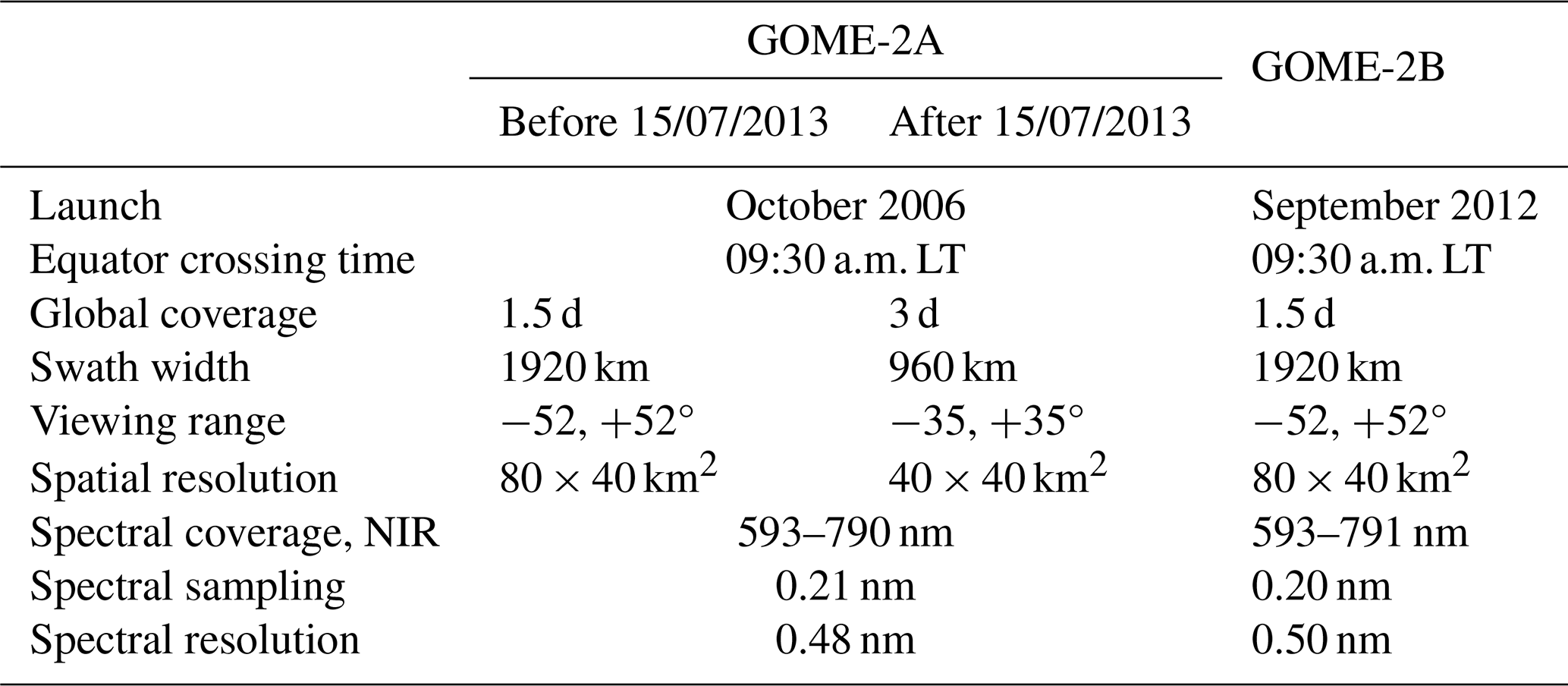
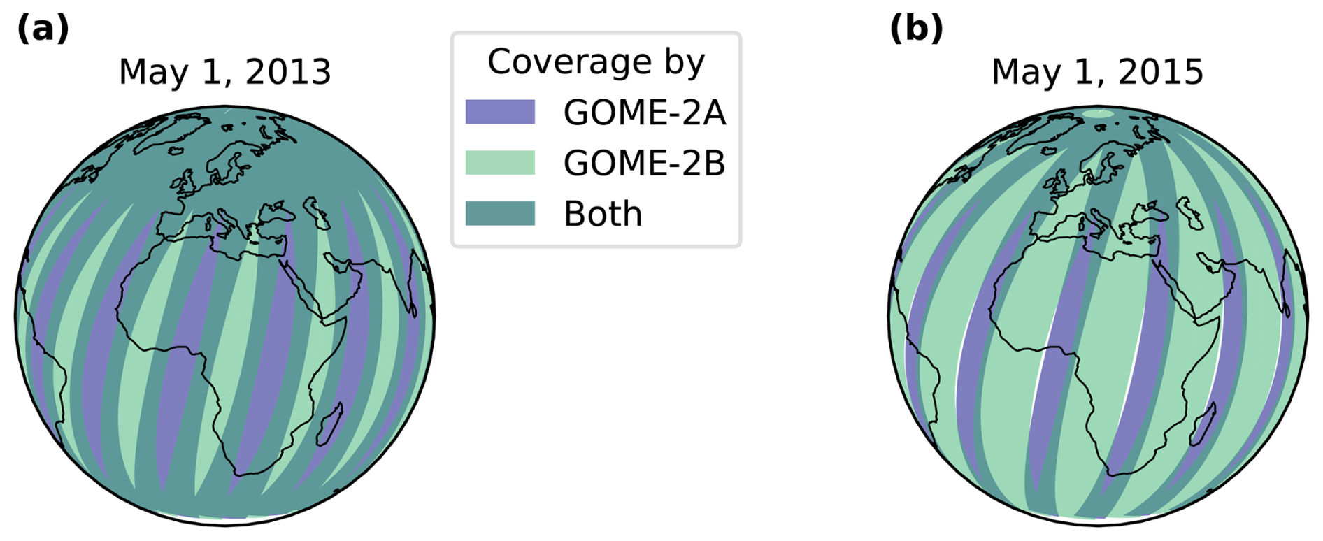
Figure 1 Coverage and overlap of GOME-2A (in blue) and GOME-2B (in green) when both are (a) in nominal swath mode and (b) in tandem mode with GOME-2A in reduced swath mode. The tandem operation started from 15 July 2013 when GOME-2B was fully operational (after the commissioning phase), and lasted until the de-orbiting of GOME-2A in 2021.

While orbital drift constrains the time window of reliable data analysis, instrumental artefacts impacted the GOME-2 observations more persistently. Specifically, the effects of instrument degradation on the observed reflectance represent a significant challenge for all three instruments. These effects exhibit varying patterns over time, occur early in operational life, and have sensor-specific characteristics (EUMETSAT, 2022). This degradation is thought to arise from build-up contamination on the scan mirror and is shown to be wavelength and scan-angle-dependent (Tilstra et al., 2012; EUMETSAT, 2022; Anema et al., 2025a). Although the shorter wavelengths are more heavily affected, the effects in the NIR can't be neglected and are known to impact the temporal consistency of SIF retrievals (Zhang et al., 2018; Gerlein-Safdi et al., 2020; Wang et al., 2022; Anema et al., 2025a).

The consistency and comparability of the individual instruments' observations are also affected by their thermal stability. Temperature variations of the optical bench along the orbit lead to changes in the spectral alignment, with noted seasonal and long-term effects (Munro et al., 2016). Additionally, these temperature variations also affect the slit function width. This variation in slit function width is believed to influence retrieved SIF values, potentially causing underestimation (false negatives) or overestimation of their magnitude (Köhler et al., 2015; Khosravi et al., 2015; van Schaik et al., 2020).

3 Application of SIFTER v3 to GOME-2B

In this study, we retrieve SIF from the GOME-2B sensor using the SIFTER v3 retrieval algorithm. The retrieval methodology and its underlying principles are kept identical to those applied to GOME-2A (Anema et al., 2025a) to secure consistency between the two datasets. For clarity, we briefly summarise the methodology before outlining the algorithm's parameter settings tailored to GOME-2B. The SIFTER v3 retrieval consists of three main steps: degradation correction of the reflectance, the SIF retrieval, and post-hoc correction for latitude bias effects. Details about the applied corrections and their impact on the alignment of GOME-2A and GOME-2B observations are provided in Sect. S1 in the Supplement.

3.1 Reflectance correction

The time, wavelength, and scan-angle dependent degradation correction is derived from analysing daily global reflectance trends over time. First, GOME-2B reflectance data for the spectral range of 712–785 nm are collected between 60° S and 60° N, and with solar zenith angles below 85°. Scenes are not filtered on cloud conditions or sun glint, but data corresponding to static or narrow swath observations are excluded. Daily averages are then obtained for scan-index s (n=24) and detector pixel at wavelength λ.

As an illustration, Fig. 2 shows the daily global reflectances at λ= 747.2 nm and s=1 and s=24 in green. Different long-term temporal reflectance patterns are observed over the easternmost (s=1) and westernmost (s=24) pixel. The reflectance over the easternmost pixel shows a clear decreasing pattern over time, whereas it remains more stable over the westernmost pixel. The stronger eastward degradation is consistent with patterns observed in GOME-2A and predecessors GOME and SCIAMACHY (Anema et al., 2025a; EUMETSAT, 2022). The degree of degradation, or signal attenuation, depends on the properties of the contamination layer that develops on the scan mirrors over time and its interaction with polarised light (EUMETSAT, 2022). Eastward light is likely more affected due to the higher degree of polarisation.

Next, we model the temporal variation in global mean reflectance ($R_{\mathit{\lambda },s}^{*}$(t)). Global mean reflectances are expected to vary seasonally due to changing geometry and scene observation. Although no major long-term trends are expected, substantial long-term trends are noted (Fig. 2). Therefore, $R_{\mathit{\lambda },s}^{*}$(t) is represented by a combination of a polynomial $P_{\mathit{\lambda },s}^p$(t) and a finite Fourier series $F_{\mathit{\lambda },s}^q$(t):

$$\begin{array}{}\text{(1)}& R_{\mathit{\lambda },s}^{*}\left(t\right)=P_{\mathit{\lambda },s}^p\left(t\right)[\mathrm{1}+F_{\mathit{\lambda },s}^q(t\left)\right]\end{array}$$

$F_{\mathit{\lambda },s}^q\left(t\right)$ and $P_{\mathit{\lambda },s}^p$(t) capture the seasonal variation and long-term trends, respectively. For GOME-2B, the Fourier order q is set to 6, and the polynomial degree p to 5. A high polynomial degree was necessary for the fit of GOME-2B reflectances to accurately capture the abrupt drop in signal from around 2020, particularly on the eastern side, as visible in Fig. 2. While geophysical changes, such as variations in cloud fraction, aerosols, and global greening, can affect long-term trends in global mean reflectance, their impact is expected to be minor compared to the observed trends and attributed impact of throughput loss following instrument degradation (Li et al., 2018; EUMETSAT, 2022). Moreover, the pronounced scan-angle dependence strongly indicates an instrumental origin.

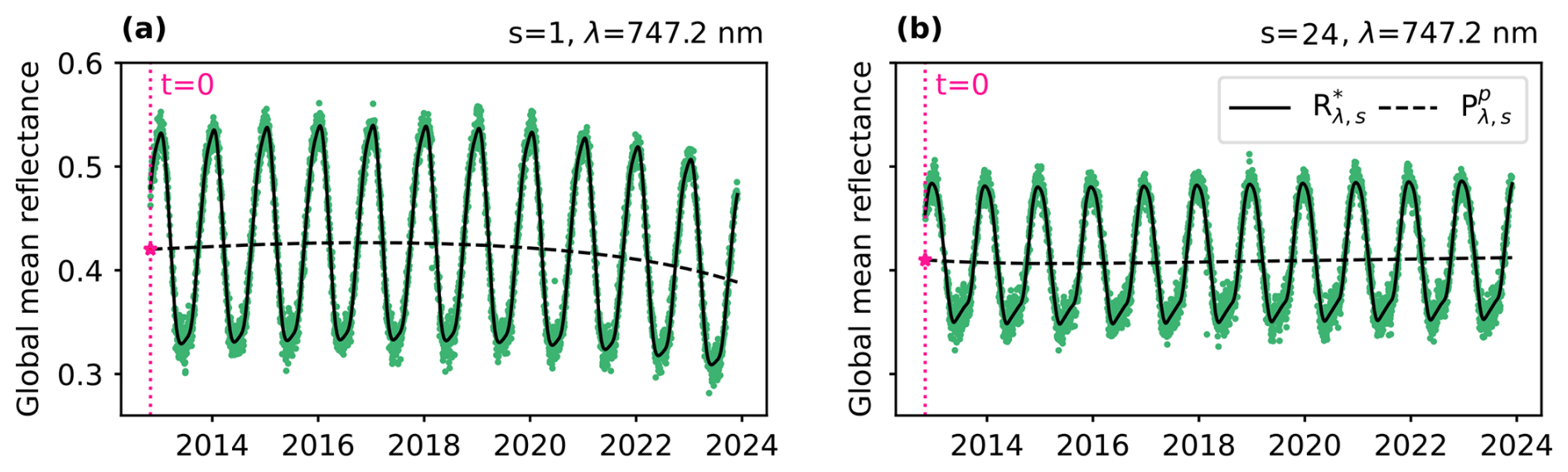
Figure 2 The observed (green dots) and fitted (solid black) global mean reflectance from GOME-2B at λ= 747.2 nm and scan-index (a) s= 1 (easternmost) and (b) s= 24 (westernmost). The dashed line shows the fitted polynomial, which captures the long-term change in the reflectance over time that is thought to be caused by the impact of instrument degradation. The reference day t₀, set at 1 November 2012, is indicated by the pink star.

To obtain the correction factors (c_λ,s(t)), Eq. (1) is fitted to the observed reflectances using least-squares regression. The obtained coefficients of the polynomial $P_{\mathit{\lambda },s}^p$ are then used to correct the long-term trends. We scale the reflectance value at day t to the value at a reference day t₀, as

$$\begin{array}{}\text{(2)}& c_{\mathit{\lambda },s}\left(t\right)=P_{\mathit{\lambda },s}^p\left(t_{\mathrm{0}}\right)/P_{\mathit{\lambda },s}^p\left(t\right)\end{array}$$

With c_λ,s(t) as correction factor at day t, wavelength λ and scan-index s. The reference day t₀ represents a day early on in the mission, assuming no spectral degradation at that time. For GOME-2B, t₀ is selected as 1 November 2012. The resulting correction factors are applied to each observed reflectance value before the SIF retrieval to counteract the identified degradation patterns.

Figure 3 shows the relative change in reflectance at ∼ 740.1 nm across the swath for multiple years, for both GOME-2A and GOME-2B. The reflectance degradation pattern represents an inconsistency in the relative loss of throughput between the observed radiance and solar irradiance. As reflectance is defined as the ratio of radiance to solar irradiance signal, a decrease in reflectance, for instance, indicates a stronger degradation of the radiance signal. In both sensors, reflectance degradation is more pronounced on the eastern side of the swath, and an increasing East-West bias develops over time. For GOME-2A, reflectances at all scanning positions increase over the first six years, then decline and eventually drop below the reference value. For GOME-2B, an overall decreasing trend in reflectances is noted.

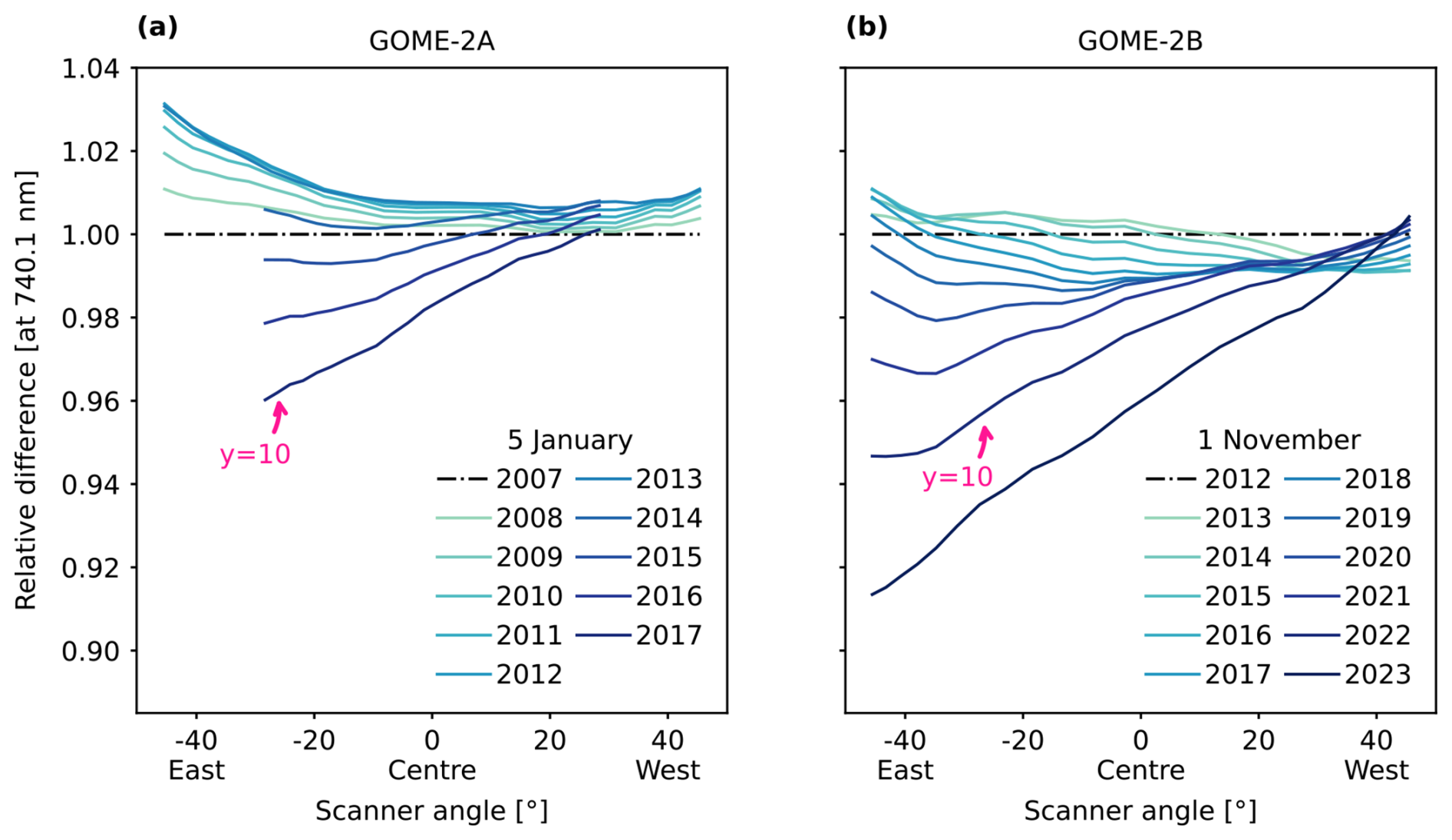
Figure 3 Reflectance degradation of (a) GOME-2A and (b) GOME-2B as a function of scanner angle for different moments and at λ= 740.1 nm. The dashed line indicates the selected reference day for each instrument, where it is expected that there is no impact of reflectance degradation (yet). The pink arrows indicate the 10th years past the reference day.

These results confirm that the reflectance degradation of GOME-2B, similar to GOME-2A (Anema et al., 2025a), is strongly scan-angle dependent and of the same order of magnitude as the temporal dependency. Importantly, the degradation trends substantially differ between sensors. Furthermore, when GOME-2B launched in 2013, GOME-2A had already drifted significantly from its original reflectance values, amplifying intersensor divergence.

3.2 SIF retrieval

The SIFTER retrieval algorithm obtains far-red SIF by making use of the relative infilling by fluorescence of solar Fraunhofer absorption lines near the 740 nm peak. A narrow retrieval window of 734 to 758 nm is used. This window represents the trade-off of minimising interference from water vapour and O₂ absorption features, while still capturing sufficient Fraunhofer lines and spectral points to ensure reliable SIF retrieval (van Schaik et al., 2020; Parazoo et al., 2019). However, some residual sensitivity due to inclusion of water vapour absorption features may remain under humid conditions. In this work, this sensitivity is reduced by using the SIFTER v3 algorithm, which includes an improved representation of atmospheric variability in the principal component construction (Anema et al., 2025c). We use the latest reprocessed level-1b dataset, Release-3 (R3), as input. The R3 dataset ensures consistent processing and auxiliary data for GOME-2A and GOME-2B up to July 2020 (EUMETSAT, 2022). From July 2020 onwards, a different processor version is used, but this is not expected to introduce significant inconsistencies in the level-1b data.

The retrieval isolates the additional vegetation fluorescence signal from atmospheric features by matching a modeled reflectance spectrum to the observed spectrum. We model the reflectance (R) using a Lambertian surface reflectance model, as described by:

$$\begin{array}{}\text{(3)}& \begin{array}{rl}R(\mathit{\lambda },\mathit{\mu },{\mathit{\mu }}_{\mathrm{0}})& \approx a_s\left(\mathit{\lambda }\right)T^{\downarrow }(\mathit{\lambda },{\mathit{\mu }}_{\mathrm{0}})T^{\uparrow }(\mathit{\lambda },\mathit{\mu })\\ & +{\displaystyle \frac{\mathit{\pi }{I}_{\mathrm{SIF}}\left(\mathit{\lambda }\right)}{E_{\mathrm{0}}\left(\mathit{\lambda }\right){\mathit{\mu }}_{\mathrm{0}}}}{T}^{\uparrow }(\mathit{\lambda },\mathit{\mu })\end{array}\end{array}$$

where μ and μ₀ are the cosines of the viewing and solar zenith angles, respectively. The surface albedo is denoted by a_s(λ), the SIF emissions from the vegetated surface by I_SIF, and the atmospheric transmission –both downwards and upwards – by T^↓ and T^↑. The modeled reflectance contains 16 unknowns, one of which is the SIF signal to be extracted. These unknowns are solved by minimising the difference between the modeled and observed R using a Levenberg-Marquardt least-squares regression (van Schaik et al., 2020; Anema et al., 2025a). Among the other 15 unknowns, five coefficients come from the surface albedo, which is estimated using a fourth-order polynomial, and ten are related to the atmospheric transmittance, which is characterised by 10 principal component (PC) functions.

The atmospheric transmittance varies with each scene and atmospheric conditions. To capture its variability, we apply principal component analysis (PCA) to a large selection of spectra across the Sahara region (16–30° N, 8° W–29° E). These observations are filtered for barren areas using land classification data to ensure the absence of vegetation and, therefore, SIF emission. We select GOME-2B spectra from five complete years (2013–2018), matching the period length used for the PC calculations of GOME-2A (2007–2012). Note that degradation corrected spectra are used (Sect. 3.1) to avoid biases. Furthermore, as introduced in SIFTER v3 (Anema et al., 2025a), the spectra are mean-centered and scaled by standard deviation before the PCA.

Figure 4 presents the first principal component (PC) for both GOME-2A and GOME-2B, and the cumulative explained variance for each PC (10 in total) for both datasets. For both sensors, PC #1 shows a similar overall structure, but the GOME-2A pattern is more sharply defined, with more pronounced features, such as deeper troughs and higher peaks. The less defined pattern in GOME-2B may reflect its generally higher reflectance uncertainty in the NIR and/or its slightly courser spectral resolution (0.5 nm vs 0.48 nm, Table 1) compared to GOME-2A. Nevertheless, the PCs capture 99.95 % of the total variance, indicating that the main spectral structures are consistently represented in both sensors.

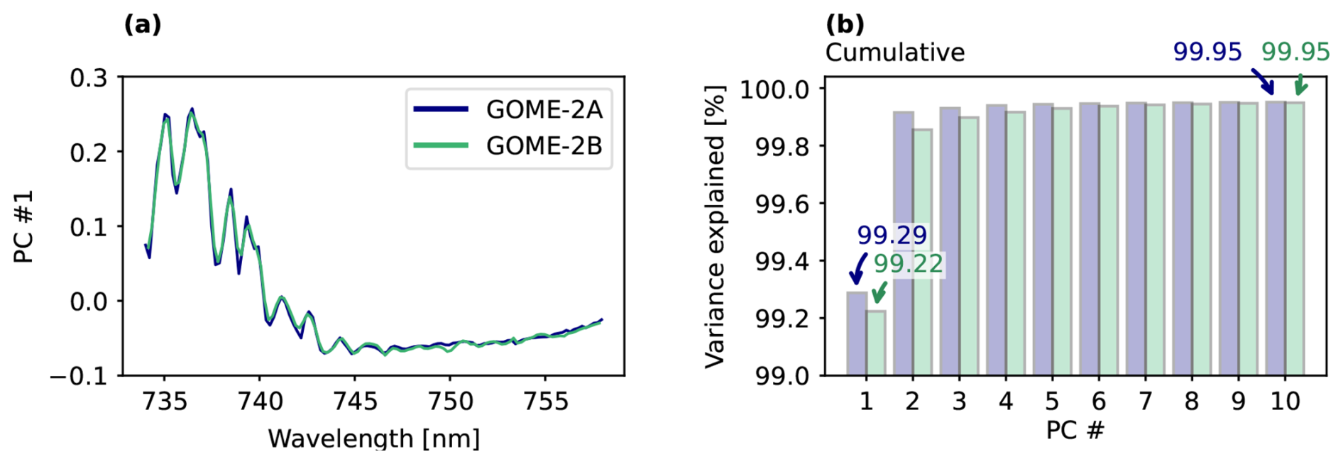
Figure 4 Panel (a) shows the leading principal component, PC #1, obtained for GOME-2A under nominal swath and GOME-2B. Panel (b) shows the cumulative explained variance of PCs 1 to 10 for both instruments. In both panels GOME-2A is shown in blue and GOME-2B is shown in green.

3.3 Latitude bias correction

The SIFTER retrieval algorithm detects the SIF signal as variations in the relative depth of Fraunhofer lines; however, instrumental artifacts can also cause false “in-filling” or “deepening” of these lines and can therefore mimic fluorescence signals (e.g. Khosravi et al., 2015; Joiner et al., 2012; van Schaik et al., 2020). These biases are latitude-dependent and may stem from temperature-driven changes in slit function width throughout the orbit, affecting the observed depth of Fraunhofer lines. Moreover, recent work by Sanghavi et al. (2025) demonstrated that rotational Raman scattering can induce seemingly large SIF values. Such effects are particularly evident over oceans and deserts, where fluorescence should be near zero, as a zero-level offset.

Figure 5 shows the zero-level offset observed in GOME-2A and GOME-2B SIF over the Pacific Ocean (130–150° W), plotted by latitude. In GOME-2A SIF, a clear annual pattern of negative SIF values is noticeable, which shifts from north to south across latitudes. Additionally, the negative offsets intensify over time, with larger negative values observed in the later years. In GOME-2B, a different pattern is noticeable with strong positive offsets appearing early in the years ranging between 20° N–20° S. Additionally, GOME-2B shows strong variation between positive and negative offsets across latitude. Due to the differing patterns observed in both instruments, SIF values from GOME-2A and GOME-2B are not directly comparable. Consequently, it is necessary to apply a correction to account for these discrepancies, reduce intersensor biases, and ensure spatial consistency within and across the datasets.

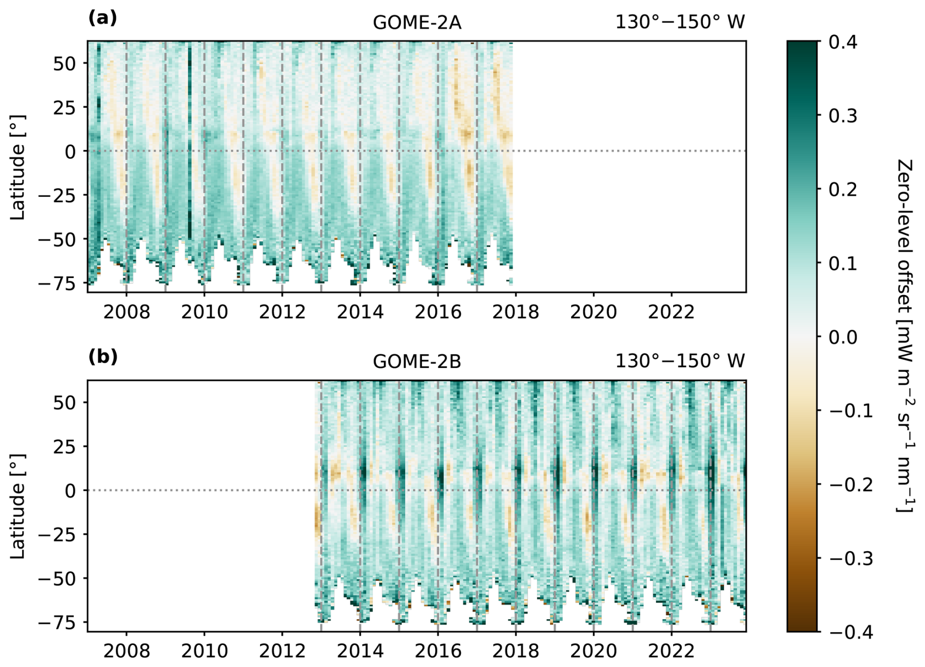
Figure 5 Observed zero-level offset of SIF retrieved from (a) GOME-2A and (b) GOME-2B across the Pacific ocean – where SIF is expected to be 0 – per latitude and over time. The SIF values shown are not adjusted for the latitude bias. The shown data are monthly averaged, gridded at 0.5° × 0.5° resolution, and subsequently averaged over 130–150° W.

To address the latitude bias effects and create higher consistency between GOME-2A and GOME-2B, we apply the post-hoc correction method from SIFTER v3 (Anema et al., 2025a). This additive correction adjusts the retrieved SIF retrieval based on daily- and latitude-specific biases observed across reference areas over the Pacific and Atlantic Ocean. The correction is characterised as a function of reflectance (at 744 nm) per latitude band and on a daily basis, thereby accounting for brightness-dependent effects. The latitude bias correction brings SIF values over the Pacific Ocean region, within the expected near-zero range for both GOME-2A and GOME-2B (shown in Fig. S3). This confirms that latitude-dependent offsets were effectively corrected for, reducing the correlated intersensor divergence.

4 Comparison of GOME-2A and GOME-2B SIF

4.1 Spatial consistency

Here, we compare the spatial distribution of SIF as retrieved from GOME-2A and GOME-2B over the period when both sensors operated in tandem. For both datasets, valid SIF data were selected and seasonally averaged over the 2013–2017 period at a 0.5° × 0.5° spatial resolution. To avoid potential biases, we excluded the GOME-2B commissioning phase and only used complete seasons.

Figure 6 shows the mean SIF retrieved from GOME-2A and GOME-2B for the December–February (DJF) and June–August (JJA) seasons. Both datasets exhibit similar spatial distributions in SIF and align strongly with each other. However, slight differences are noted. GOME-2B SIF tends to be more negative over barren areas, such as Western China. Moreover, on average, GOME-2B SIF values exceed those of GOME-2A SIF by approximately 5 %–6 %. This positive bias appears to be most pronounced in regions with high vegetation activity, such as the Corn Belt region in JJA and the Amazon in DJF.

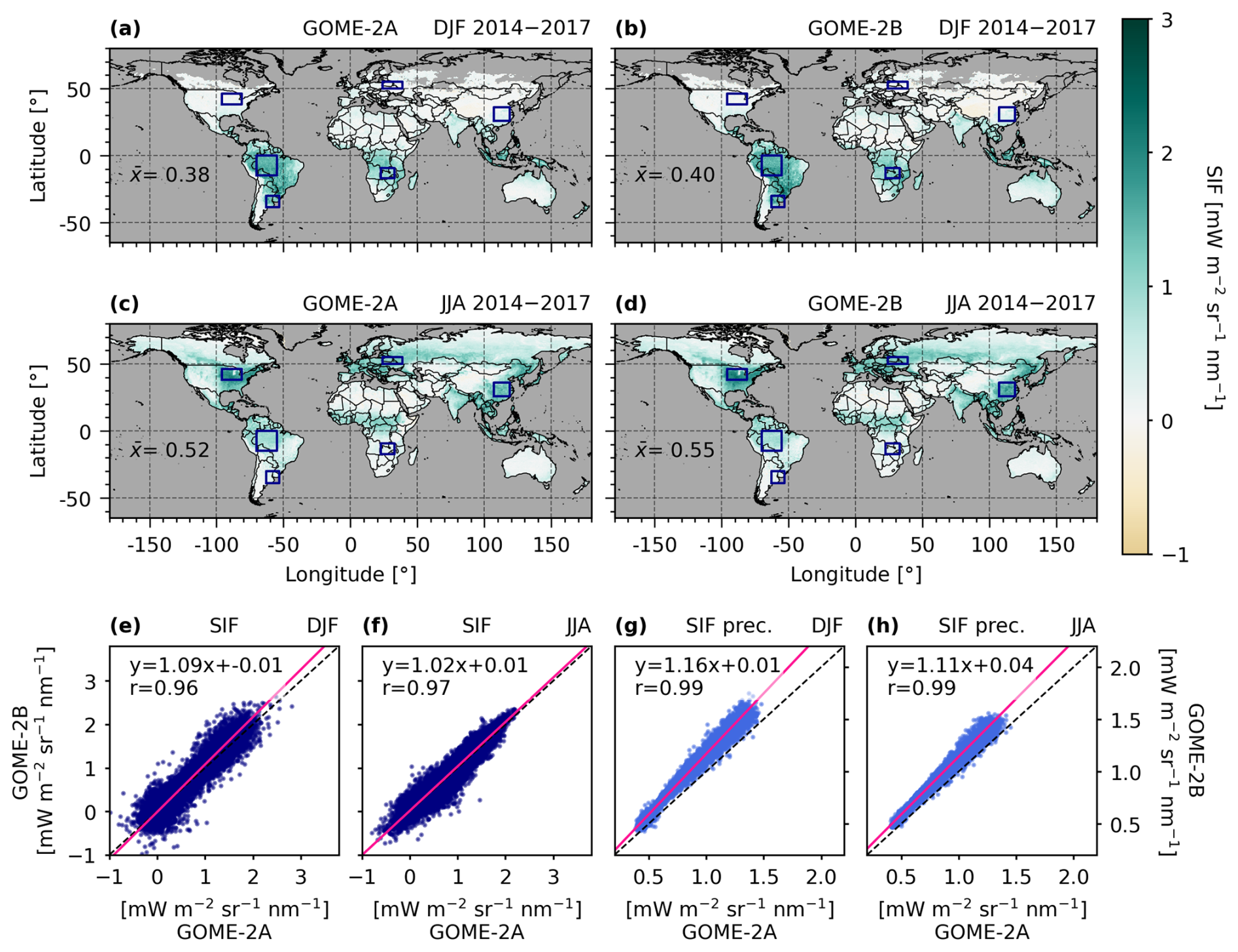
Figure 6 Seasonal averaged GOME-2A and GOME-2B SIF over December–February (DJF), and June–August (JJA) 2014–2017. DJF includes December of the preceding year, e.g., DJF 2014 includes December 2013. Panels (e) and (f) show the correlation between GOME-2A and GOME-2B SIF for these periods; panels (g) and (h) show the correlation between their respective uncertainty. Major axis regressions are used for the correlations (pink line). Only land pixels are shown and presented to focus on biosphere-relevant differences. SIF values are filtered for cloud fractions < 0.3 (FRESCO+ v2) and gridded at 0.5° × 0.5°. The blue rectangles mark selected study regions.

Aside from the differences in SIF values, GOME-2B also shows consistently higher uncertainty in SIF than GOME-2A, on the order of 17 %–18 %. This likely reflects a combination of larger uncertainties in the input reflectance, lower spectral resolution (Table 1), and the less sharply defined principal components (Fig. 4), all of which can propagate through the retrieval and increase the final uncertainty.

Overall, GOME-2A and GOME-2B SIF values agree well with consistent spatial patterns and strong correlations (r=0.96 for JJA, and r=0.97 for DJF). These results indicate coherence between both datasets. Nonetheless, GOME-2B SIF values are slightly but systematically biased against GOME-2A SIF values. In the following subsections, we examine to what extent this divergence reflects true biases or results from sampling differences.

4.2 Impact of viewing geometry differences

During the operational tandem phase, GOME-2A and GOME-2B operated under different swath configurations. The swath reduction of GOME-2A limited the viewing zenith angle (VZA) range of the observations from ∈ [−52, +52°] to [−35, +35°] (Table 1). As a result, the GOME-2B SIF averages shown in Fig. 6 include observations made under larger VZA angles (|VZA| > 35°) than GOME-2A. To understand how these discrepancies in viewing geometry might induce biases between GOME-2A and GOME-2B SIF, we first discuss the principle behind the angular dependence of SIF observations.

The SIF signal detected by the satellite sensor reflects the fraction of total emitted chlorophyll fluorescence that escaped the canopy and reached the sensor. This fraction depends on the photon scattering, leaf properties, and canopy architecture, influencing the propagation of SIF photons through the canopy (e.g., van Wittenberghe et al., 2015; Peltoniemi et al., 2005; Joiner et al., 2020; Sun et al., 2023). As a result, the SIF signal is anisotropic and therefore depends on the viewing geometry between the Sun, vegetation, and the satellite sensor (e.g. Yang and van der Tol, 2018; van Wittenberghe et al., 2015; Dechant et al., 2020).

Figure 7 illustrates the scan and illumination dependencies of the observed SIF by GOME-2. In the following, we describe each individual mechanism contributing to these dependencies on SIF. The relative importance of these mechanisms depend on the conditions, such as canopy structure and illumination geometry. At nadir, the sensor mainly detects photons emitted from the top of the canopy. Toward the swath edges, at larger viewing zenith angles (VZA), the sensor observes the canopy from a slanted angle, thereby enhancing the probability of detecting photons originating deeper within the canopy. Moreover, the viewing perspective determines whether the sunlit or shaded side of the canopy is viewed, leading to higher or lower observed values, respectively. For GOME-2A observations, the western ground pixels are typically sunlit, whereas eastern ground pixels tend to be shaded.

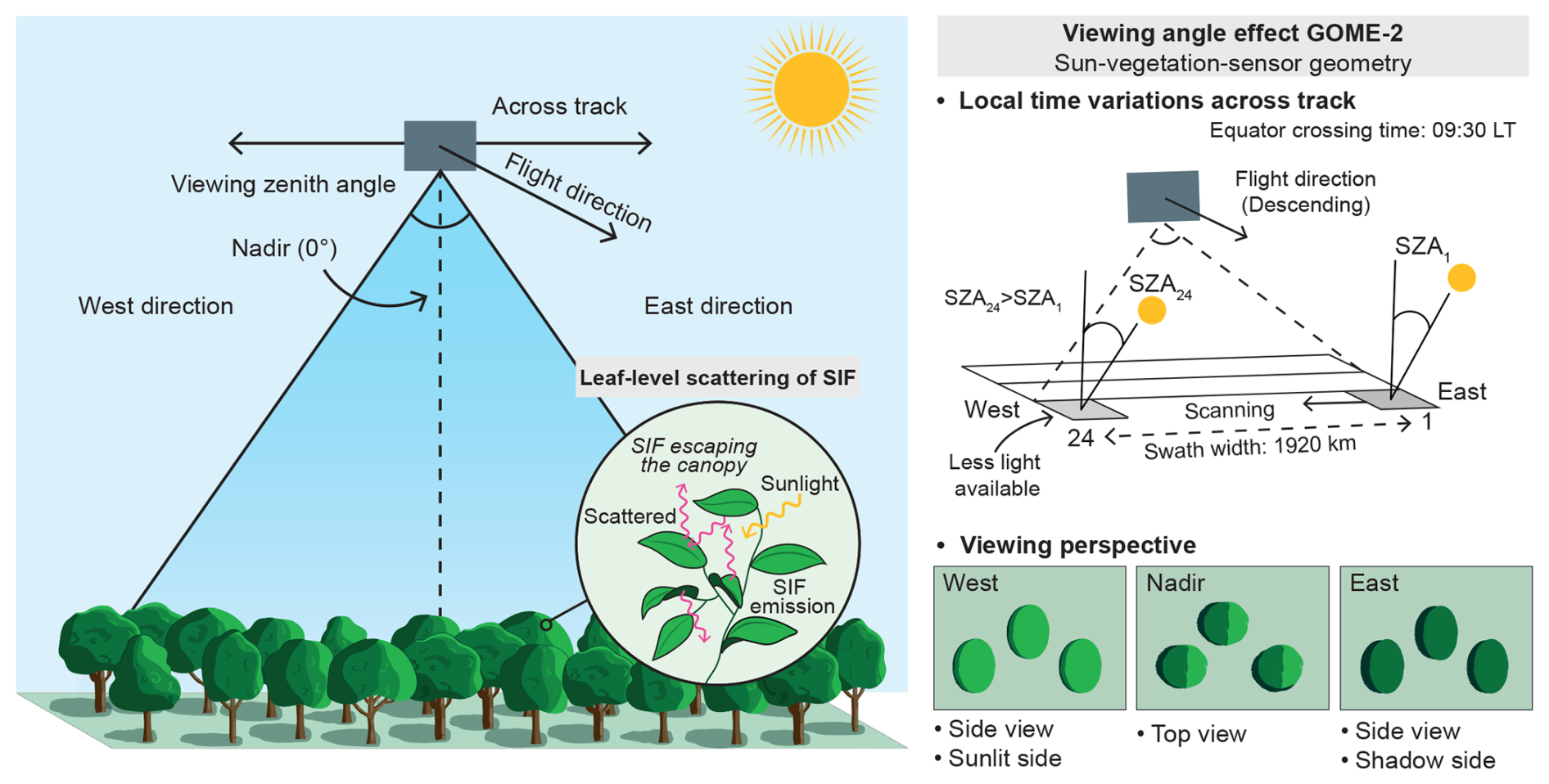
Figure 7 Schematic of the scan-angle dependencies of GOME-2 SIF observations. The instrument scans from east (pixel 1) to west (pixel 24), with a total scanning time of around 50 min.

Wide-swath instruments, such as GOME-2 and TROPOMI, also introduce across-track variations in incoming solar irradiance (Joiner et al., 2020). The wide swaths cover an extensive longitudinal range that spans different local solar times and thus solar zenith angles (SZA). As a result, GOME-2 observes eastern pixels later in the morning when solar illumination is typically higher (lower SZA), leading to potentially higher SIF values. Together, these viewing geometry factors can lead to systematic asymmetry in the observed SIF values across-track (Joiner et al., 2020). The geometry effects on observed SIF are well known, and SIF is generally averaged over a sufficient number of observations to mitigate these effects (e.g. Turner et al., 2021).

To assess the effect of discrepancy in viewing geometry between GOME-2A and GOME-2B, we average both datasets across scan positions. Figure 8 shows seasonal SIF as a function of VZA for both sensors across various geographical regions. A consistent across-track asymmetry is observed in all regions during the peak seasons, specifically JJA in the Northern Hemisphere and DJF in the Southern Hemisphere. During these high activity seasons, large SIF values near the eastern and, more prominently, the western edges of GOME-2B's 1920 km swath contribute to a higher overall average (${\stackrel{\mathrm{‾}}{x}}_{\mathrm{B}}$), compared to GOME-2A SIF (${\stackrel{\mathrm{‾}}{x}}_{\mathrm{A}}$). For instance, GOME-2B SIF has a bias of 13.9 % compared to GOME-2A SIF over Zambia. SIF values from both sensors align well when restricted to the shared VZA range of [−35, +35°]. The largest divergence across-track emerges when the |VZA| exceeds ∼ 30°. Within GOME-2B's wide swath, westward pixels can exhibit up to 35 % higher SIF values than eastward pixels during peak seasons (see Sect. S2.2 for more detail).

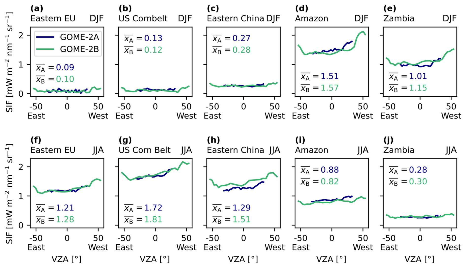
Figure 8 Seasonally averaged SIF from GOME-2A (blue) and GOME-2B (green) across the viewing zenith angle (in °). Showing seasonal SIF for June–August (JJA) 2014–2017 (top plots) and December–February (DJF) 2014–2017 (bottom plots), over Eastern Europe, the United States Corn Belt, Eastern China, the Amazon, and Zambia.

Figure 9 shows zonal averages of SIF from GOME-2A (in solid blue), GOME-2B using observations from the full VZA range (in solid green), and VZA ranges matched with GOME-2A (in dashed green). Overall, GOME-2A and GOME-2B SIF values converge when their VZA ranges match. For instance, the difference in DJF SIF between GOME-2A and GOME-2B over 0 to 40° S decreased from 13.8 % to 4.9 %. These results indicate that a significant portion of the inter-sensor differences in SIF can be attributed to variations in VZA sampling. Nonetheless, some divergence between GOME-2A and GOME-2B SIF remains. The remaining biases may result from differences in spatial and temporal sampling, as well as from differences in sensor and orbit characteristics.

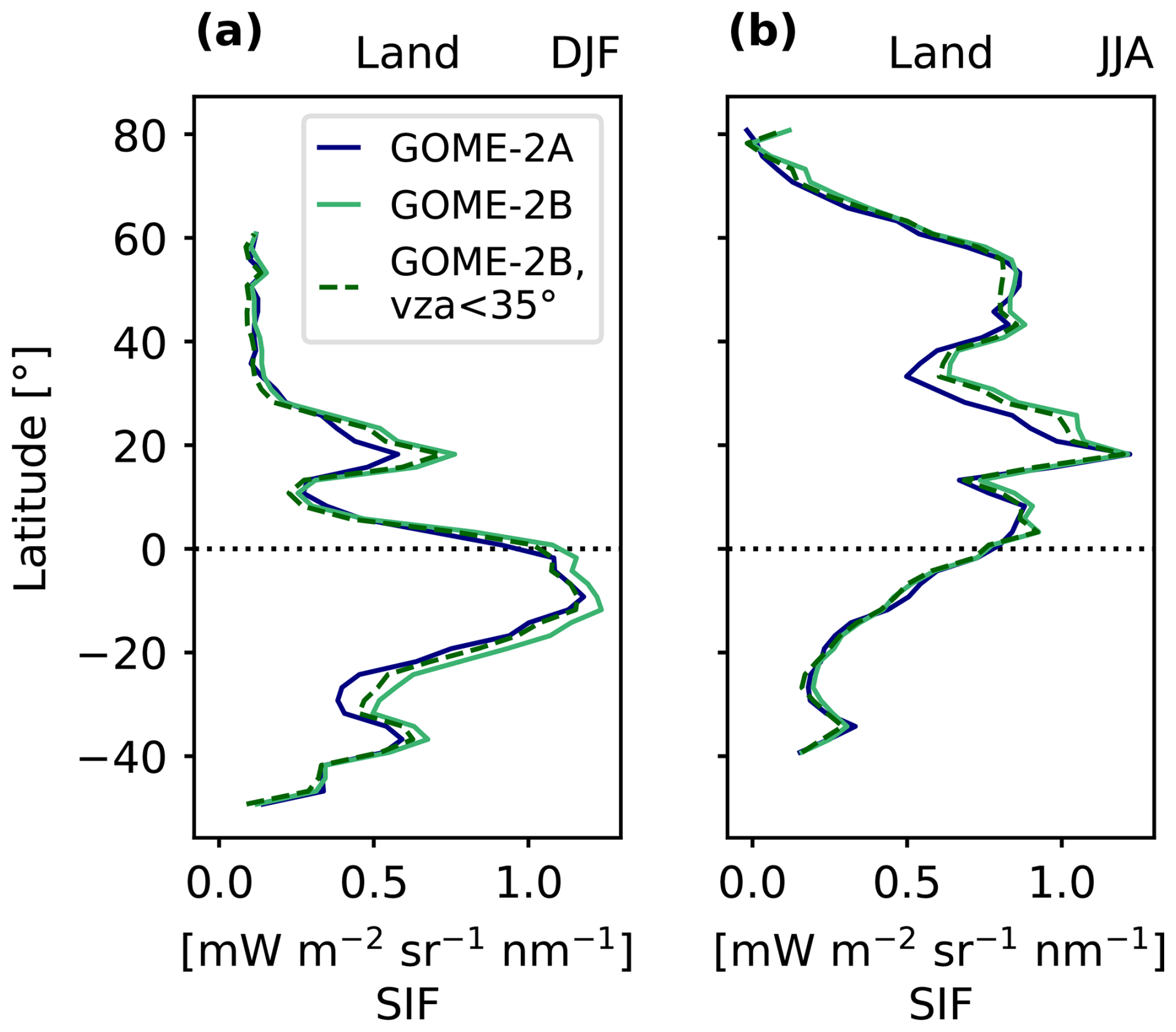
Figure 9 Zonal averaged SIF from GOME-2A (solid blue line), GOME-2B considering all observations (solid green line), and only those with |VZA| < 35 ° (dashed green line), for (a) DJF 2016 and (b) JJA 2016. Zonal averages reflect all land pixels. Pixels over the Sahara region (15–32° N, 16° W–52° E) were filtered to limit distortion of observations over desert areas and focus primarily on vegetated regions. The SIF values are plotted by latitude at 2° resolution.

4.3 Isolating sensor-specific differences

To further evaluate the divergence between GOME-2A and GOME-2B SIF, we perform two co-sampling experiments (see Sect. S2.3). In Experiment 1, GOME-2A and GOME-2B pixels are spatially and temporally collocated. Matching pixel pairs had a maximum 50 km distance between their centers, at least 60 % spatial overlap of the smaller GOME-2A pixel with the GOME-2B pixel, and observation times less than 50 min apart. Experiment 2 applies the same constraints, with an additional requirement that both observations are within the same viewing geometry range of [−35, +35°]. These constraints help to isolate instrument-specific biases from those arising from sampling mismatches. Due to the limited spatial overlap of GOME-2A and GOME-2B ground pixels, sampling in Experiment 2 is practically limited to the Northern latitudes.

Figure 10 shows GOME-2A and GOME-2B SIF data, sampled to both experiments accordingly, and averaged over JJA 2014–2017. GOME-2A and GOME-2B SIF are better aligned for Experiment 2 (1.9 % bias) than for Experiment 1 (5.6 % bias) – as expected. This is confirmed by the empirical cumulative distribution functions (ECDFs) (bottom plots in Fig. 10). ECDFs visualise the cumulative distribution of each dataset, enabling clear detection of systematic shifts between datasets. When only spatially and temporally co-sampled, Exp. 1, GOME-2B SIF values at the 90th percentile are 7.1 % higher than the corresponding GOME-2A value. Including co-sampling of viewing angles, Exp. 2, reduces the bias of GOME-2B SIF to GOME-2A SIF to 2.1 %.

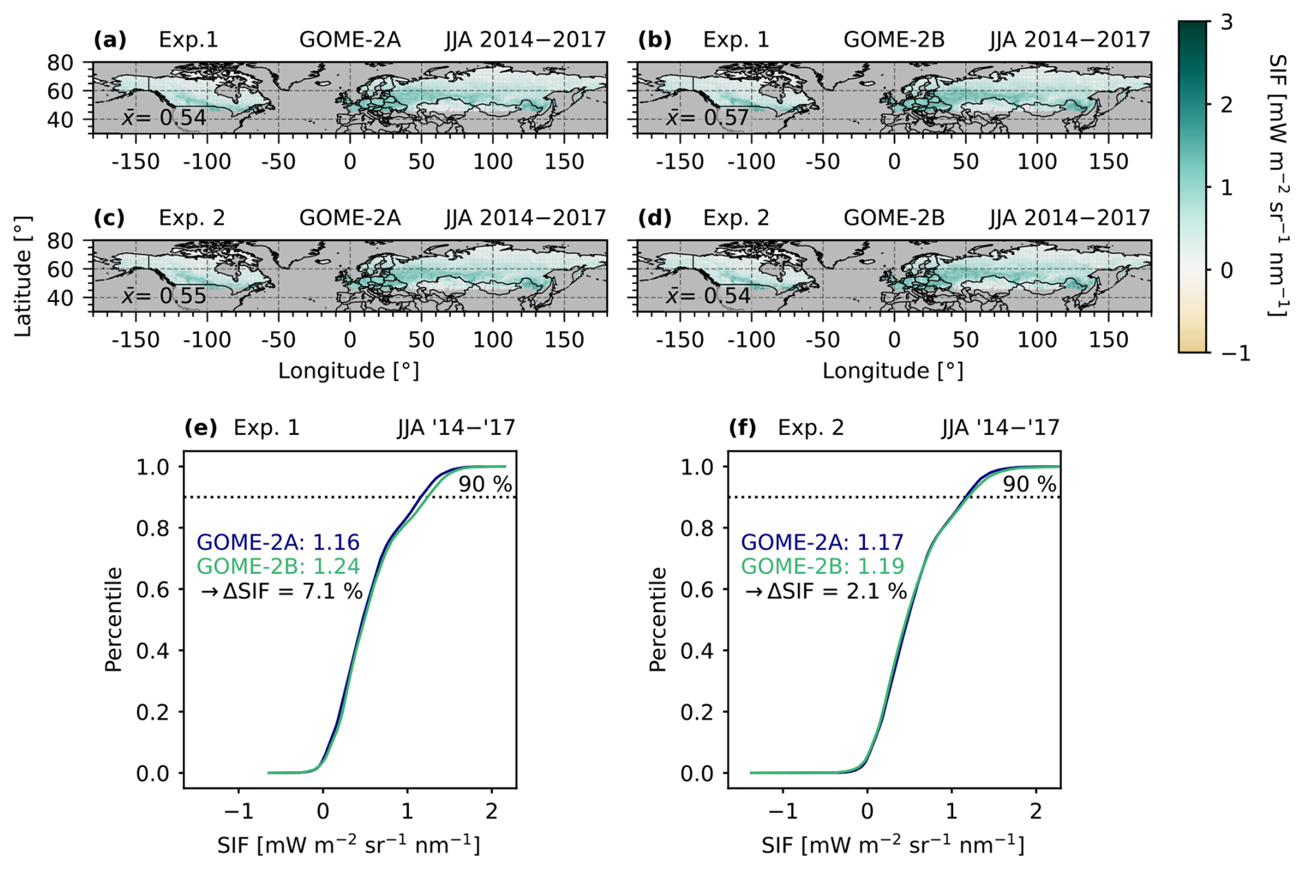
Figure 10 (a, c) GOME-2A and (b, d) GOME-2B sampled according to Experiments 1 and 2, averaged over June–August (JJA) from 2014 to 2017 on a 0.5° × 0.5° grid. SIF values are shown for grid cells with valid and sufficient observations (exceeding the 10th percentile of data counts) in both datasets and experiments. The mean SIF is shown as $\stackrel{\mathrm{‾}}{x}$. The two bottom panels show the ECDF plots of GOME-2A and GOME-2B SIF according to (e) Experiment 1 and (f) Experiment 2. The dotted line indicates the 90th percentile, with the text indicating the corresponding SIF values.

Despite the reduced structural bias in Experiment 2, the correlation between GOME-2A and GOME-2B SIF is lower (r=0.92) than in Experiment 1 (r=0.97) (shown in Fig. S13). However, the SIF averages corresponding to Experiment 1 are based on nearly three times as many observations per grid cell as those in Experiment 2. This discrepancy in data density between the two experiments might reduce the comparability of their results. To enable a more balanced comparison, we constructed a reduced version of Experiment 1. The additional test involved averaging Experiment 1 data over a randomly selected subset of days from the JJA 2014–2017 period to match the data density of Experiment 2 better. The comparison between this reduced Experiment 1 and Experiment 2 was performed using only grid cells with valid and sufficient observations in both experiments. The divergence between GOME-2A and GOME-2B SIF remained similar to that of Fig. 10, but the correlation between GOME-2A and GOME-2B SIF for Experiment 2 (r=0.96) now exceeds that of Experiment 1 (r=0.95) (shown in Fig. S16). These results confirm that the co-sampling requirements as set in Experiment 2 result in the best agreement among GOME-2A and GOME-2B SIF. The details on this additional test are in Sect. S2.3.1.

GOME-2A and GOME-2B SIF show strong coherence in terms of spatial distribution. However, our results indicate the importance of similar sampling to reduce systematic biases between the two datasets. Particularly, discrepancies in viewing geometry sampling have been shown to distort the coherence between inter-sensor SIF datasets. When both datasets are sampled similarly, GOME-2A and GOME-2B SIF agree to within 2 %. A slight discrepancy is expected, as they are separate sensors with minor differences in instrumental characteristics (Table 1). These results provide confidence in the consistency of GOME-2A SIF (pre-July 2013) and GOME-2B SIF (from July 2013 onwards), when both sensors operated with the same 1920 km swath and viewing zenith angle ranges (VZA ∈ [−52, +52°]).

5 Long-term time series analysis

This section evaluates the combined 2007–2023 GOME-2 SIF record over time. It uses GOME-2A data from January 2007 to June 2013 and GOME-2B data from July 2013 onwards. We focus on SIF observations from the GOME-2A instrument under its nominal swath configuration to ensure similar viewing angle ranges within both datasets, limiting the bias between GOME-2A and GOME-2B SIF and advancing their connection (as found in Sect. 4.3). The record's performance is evaluated in two ways. First, the coherence between GOME-2A and GOME-2B SIF is assessed in Sect. 5.1 using statistical tests and analysis. In Sect. 5.2, the temporal consistency of the record is evaluated using independent datasets. Both analyses use monthly-averaged SIF across six vegetative regions. The monthly and spatial averaging mitigate the effects of variation in geometry on SIF.

5.1 Temporal coherence of GOME-2A and GOME-2B SIF

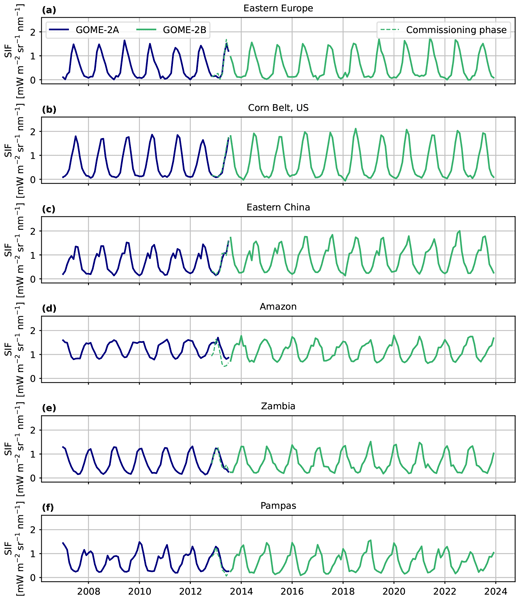
Figure 11 shows the monthly regional averages of SIF from January 2007 to December 2023. For most regions, the transition from GOME-2A SIF (in blue) to GOME-2B SIF (in green) appears seamless. However, in the Amazon, a slight downward shift in GOME-2B SIF, relative to GOME-2A SIF, is noted. To test whether this shift is related to the instrument transition, we proceed with statistical and analytical tests.

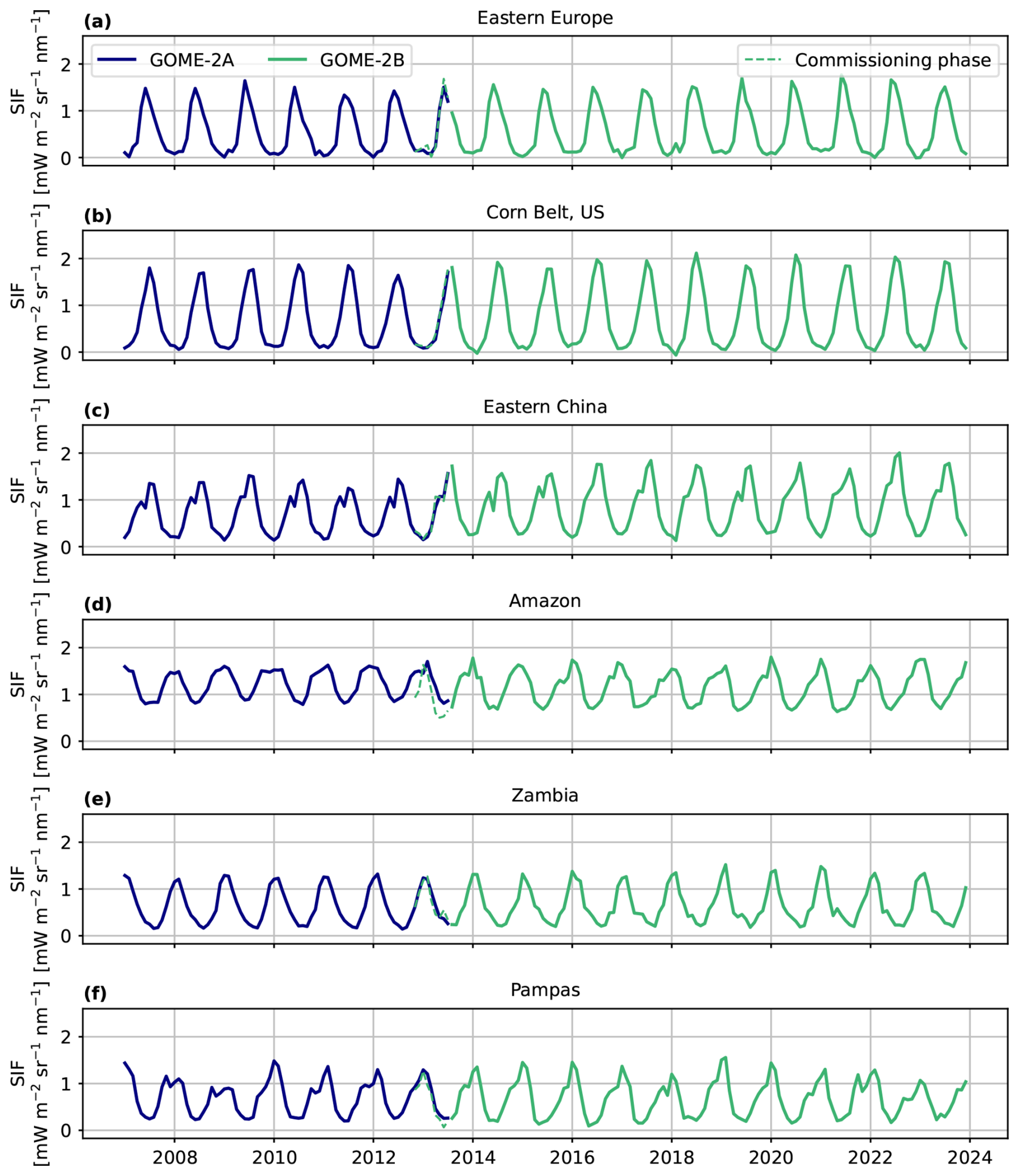
Figure 11 Time series of monthly averaged Level-2 SIF values retrieved from GOME-2A (in blue) and GOME-2B (in green) over (a) Eastern Europe, (b) the United States Cornbelt, (c) Eastern China, (d) the Amazon, (e) the Congo Basin, and (f) the Pampas region. GOME-2B SIF observations during the instrument's commissioning phase are indicated by the dashed green line.

To statistically investigate whether a structural break occurs at the transition month T₀, July 2013, from GOME-2A to GOME-2B SIF data, we fit a simple model to the monthly SIF time series, which includes a linear trend (αt), seasonal component (S_t), and a mean level shift term (δU_t):

$$\begin{array}{}\text{(4)}& y_t=\mathit{\mu }+\mathit{\alpha }t+S_t+\mathit{\delta }{U}_t+{\mathit{\epsilon }}_t\end{array}$$

where y_t represents the regional SIF value at month t, μ the monthly mean and ε_t the residual of the observed and fitted SIF. This equation is adapted from Weatherhead et al. (1998) and commonly used to model trends in environmental variables that include a sudden level shift (e.g. van der A et al., 2006). The seasonal component S_t represents the annual cycle of SIF as a first-order harmonic:

$$\begin{array}{}\text{(5)}& S_t={\mathit{\beta }}_{\mathrm{1}}\sin \left({\displaystyle \frac{\mathrm{2}\mathit{\pi }(t-\mathit{\varphi })}{\mathrm{12}}}\right)+{\mathit{\beta }}_{\mathrm{2}}\cos \left({\displaystyle \frac{\mathrm{2}\mathit{\pi }(t-\mathit{\varphi })}{\mathrm{12}}}\right)\end{array}$$

where β₁ and β₂ control the amplitude, ϕ is the phase shift, and the angular frequency corresponds to annual periodicity.

Before fitting the full model, the phase shift ϕ is fixed through a pre-optimalisation step. We estimated its value by evaluating the model with 100 evenly spaced values of ϕ, ranging from 0 to 1, and selecting the value under which the model performs best. This ensures good alignment of the modelled SIF with the real seasonal timing and avoids non-linearity in the model.

The possible offset in GOME-2 SIF related to the moment when the time series shifts from GOME-2A to GOME-2B data in July 2013, or T₀, is accounted for by the step-change indicator U_t as:

$$\begin{array}{}\text{(6)}& U_t=\left\{\begin{array}{ll}\mathrm{0},& \text{if }t<T_{\mathrm{0}}\\ \mathrm{1},& \text{if }t\ge T_{\mathrm{0}}\end{array}\right.\end{array}$$

In this equation, U_t is set to 0 during the GOME-2A period (January 2007–June 2013) and switches to 1 from July 2013 onwards during the GOME-2B period. Finally, Ordinary Least Squares (OLS) regression is used to fit the five remaining unknowns: μ, α, β₁, β₂, and δ.

We use the fitted coefficient δ and its p-value to evaluate the existence and magnitude of any step change at transition T₀. Additionally, we apply both the Chow and the Likelihood Ratio (LR) test to evaluate the statistical significance of the potential break. The Chow test evaluates whether regression parameters differ before and after the breakpoint. It tests if the data structure is best described with one or two regressions by fitting the same model to (i) the full GOME-2 dataset, (ii) the data before T₀ (GOME-2A), and (iii) the data after T₀ (GOME-2B). The LR test complements this by comparing the regression results from the full model (including the δU_t term) with a reduced model that excludes the step-change term. A significant p-value from the LR test indicates that including the step-change term significantly improved the fit.

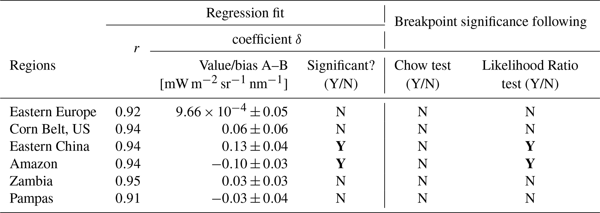
Table 2 shows the fit and statistical test results for all cases. The modelled and observed SIF are strongly correlated (r≥ 0.91), implying that the model in Eq. (4) effectively captures the seasonal patterns and long-term trends necessary to detect structural breaks. In most regions, the step change coefficient δ is insignificant, indicating no jump in SIF from T₀. However, significant step changes (p<0.05) are detected within the records across Eastern China and the Amazon. This bias is 0.13 ± 0.04 mW m⁻² sr⁻¹ nm⁻¹ over Eastern China and −0.10 ± 0.03 mW m⁻² sr⁻¹ nm⁻¹ over the Amazon region, respectively reflecting 16.6 % and 8.9 % of monthly averaged SIF over 2007–2023.

Table 2 Results of the regression fit, Chow test, and Likelihood Ratio (LR) test. The given uncertainty in δ represents one standard deviation of the estimated coefficient. The column r provides the Pearson correlation between the model fit and the monthly SIF time series. Significance is indicated by “Y” (yes) when the coefficient or test is statistically significant at the 95 % confidence level with p<0.05. If the p value exceeds 0.05, “N” (no) is indicated. For clarity, “Y” is shown in bold. More detailed results of the regression fit is shown in Table S5, and the results of the Chow and LR test are summarised in Table S6.

To interpret the detected offset bias δ, we evaluate its magnitude against the underlying uncertainty in SIF. Uncertainty in SIF retrieval can be distinguished into random errors and systematic errors. The first vary stochastically, arise from, for example, fit residual noise or sampling divergence, and decrease through averaging. Due to the spatial and temporal averaging applied here, random errors are small relative to the detected offsets. Systematic errors originate from algorithmic settings and persist despite averaging (Jacob et al., 2016). To obtain a first-order estimate of these systematic errors, independently of regional offsets, we performed sensitivity tests over the Congo Basin, a region previously used as a sensitivity testbed by Anema et al. (2025a). We perturbed the settings of four distinct retrieval steps: (i) the degradation correction, (ii) the PC's, (iii) the interpolation across the slit function (discussed in more detail in Anema et al. (2025a)), and (iv) the latitude bias correction to assess their sensitivity. The largest sensitivity arises from the PCs used within the fitting model, particularly the number of PCs chosen to represent the atmospheric transmission. Varying the number of PC's from 10 to 6 led to a divergence of 0.47 mW m⁻² sr⁻¹ nm⁻¹ for GOME-2B SIF at 14 January 2017 over the Congo Basin. Combining the uncertainties from the four perturbed retrieval settings gives an illustrative value of 0.55 mW m⁻² sr⁻¹ nm⁻¹. Retrieval sensitivities of comparable order are expected in other regions, including Eastern China and the Amazon. Details on these tests are provided in Sect. S5.

The offsets δ detected in Eastern China (+0.13) and the Amazon (−0.10) are smaller than the estimated systematic error of 0.55 mW m⁻² sr⁻¹ nm⁻¹. This indicates that the offsets lie within the range of retrieval sensitivities, but they nevertheless represent a persistent inter-sensor difference. Additionally, the LR test confirms that the addition of an offset term enhances the model fit for these two regions (Table 2). On the other hand, the Chow test results suggest the regression parameters remain consistent over the full GOME-2 record. These results imply that, while there is confidence in a mean-level bias at T₀, the seasonal pattern and structure did not differ significantly before and after July 2013. Therefore, we add the found δ magnitudes as a correction term to the monthly regional SIF values during the GOME-2B period (from July 2013 onward) to align the records of GOME-2A and GOME-2B and support the use of both records as one consistent record. The corrected time series for Eastern China and the Amazon are shown and evaluated in Sect. 5.2. Both regions are characterised by higher atmospheric humidity. The enhanced retrieval sensitivity under such conditions may contribute to the observed intersensor difference. A full attribution of these remaining differences, however, is beyond the scope of this study and requires further investigation.

Finally, we verify the impact of the correction on the record's coherence by using an independent dataset as a reference. Specifically, we use FluxSat GPP data, which overlaps with the analysed period from January 2007 to December 2020 (Joiner et al., 2018). FluxSat GPP is a satellite-derived global product that uses geometry-adjusted, daily-scaled MODIS MCD43D reflectance data and a machine learning approach to upscale eddy-covariance flux measurements from FLUXNET 2015. Assuming that FluxSat GPP correlates with SIF similarly across both sensors, it serves as a common reference to reveal intersensor biases. Each dataset – GOME-2 SIF with/without intersensor offset correction, and FluxSat GPP – is standardised over January 2007–December 2020 to enable cross-evaluation of their temporal variability. The standardisation relates the temporal variability to the data's standard deviation. We then compare the average difference between GOME-2 SIF and FluxSat GPP before and from T₀ (July 2013), using both uncorrected and GOME-2 SIF corrected for the detected intersensor offset. The period before T₀ covers January 2007 to June 2013, and the period from T₀ covers July 2013 to December 2020.

Figure 12 shows the improvement in temporal consistency between GOME-2 SIF and FluxSat GPP over Eastern China and the Amazon after applying the intersensor offset correction. Before the correction, or the alignment of GOME-2A and GOME-2B SIF, the mean difference in SIF and GPP shifts substantially around T₀. Since the datasets are standardised, this shift in SIF−GPP directly reflects the divergence between GOME-2A (<T₀, January 2007–June 2013) and GOME-2B SIF (≥T₀, July 2013–December 2020) as a fraction of the total variability over time. For example, the alignment of SIF from both sensors reduced their divergence from 27.7 % to 4.6 % of the total variability over the Amazon region – a reduction of 23.1 %. This confirms that the application of the intersensor offset correction enhanced the temporal consistency within the combined GOME-2 record. Note that remaining differences around T₀ (July 2013) may also reflect changes in the SIF–GPP relationships due to changed environmental conditions over time.

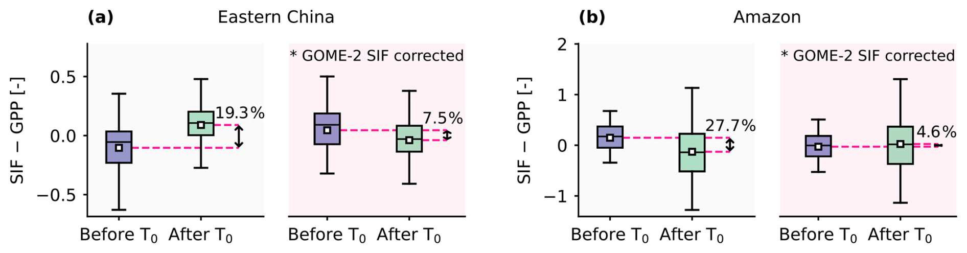
Figure 12 Differences in standardised FluxSat GPP and standardised GOME-2 SIF over the period before T₀ (January 2007 to June 2013) and after T₀ (July 2013 to December 2020). Each monthly averaged dataset is standardised by subtracting its mean value (μ) from each value (x₀) and dividing it by its standard deviation (σ); then $x=(x_{\mathrm{0}}-\mathit{\mu })/\mathit{\sigma }$. T₀ represents the transition of GOME-2A to GOME-2B SIF in July 2013. The box plots on the right, plotted against a pink background, show the difference between the intersensor offset corrected GOME-2 SIF and FluxSat GPP. The black arrows indicate the difference between averaged SIF−GPP before and after T₀, with the numbers indicating this difference as a percentage of total variability over the 2007–2020 period. The SIF−GPP differences are shown over (a) Eastern China and (b) the Amazon.

Overall, the presented approach to detect and correct for intersensor biases seems effective in enhancing the record's coherence. The methodology shown in this section can be used as a framework to detect, assess, and correct for potential biases between GOME-2A and GOME-2B SIF time series.

5.2 Evaluation of GOME-2 SIF against independent datasets

To evaluate whether the combined GOME-2 SIF records consistently track vegetation activity, we compared them to independent satellite-based proxies for photosynthesis: FluxSat GPP (Joiner et al., 2018) and TROPOMI SIF data obtained by Köhler et al. (2018). Since TROPOMI SIF data is available from early 2018, it is explicitly used for cross-evaluation against the GOME-2B SIF period. Both datasets are widely used to track inter-annual vegetation dynamics. True validation of SIF observation is restricted due to the lack of ground truth. Direct in situ validation is limited due to the mismatch in spatial resolution and the dependence of SIF values on observation time, viewing geometry, and the instrument's spectral characteristics (Mohammed et al., 2019). Therefore, cross-comparison with established independent datasets provides the common practice (e.g., Joiner et al., 2016; Köhler et al., 2018, 2015; Anema et al., 2025a). The correlations between GOME-2 SIF and independent data are shown in Sect. S4.

Figure 13 shows the regional monthly time series of GOME-2 SIF, TROPOMI SIF, and FluxSat GPP, with GOME-2 SIF corrected for intersensor offsets in Eastern China and the Amazon (Sect. 5.1). All datasets were standardised to enable comparison. Across all regions, GOME-2 SIF consistently follows the seasonal cycle of FluxSat GPP with high correlations of r≥ 0.98 outside the Amazon and r=0.92 over the Amazon. The application of the intersensor offset correction showed a positive impact on these correlations with an increase from r= 0.97 to r=0.98 over Eastern China and from r= 0.91 to r= 0.92 over the Amazon (shown in Fig. S20). Although these improvements are modest, they nonetheless suggest that applying the bias correction enhances the temporal consistency.

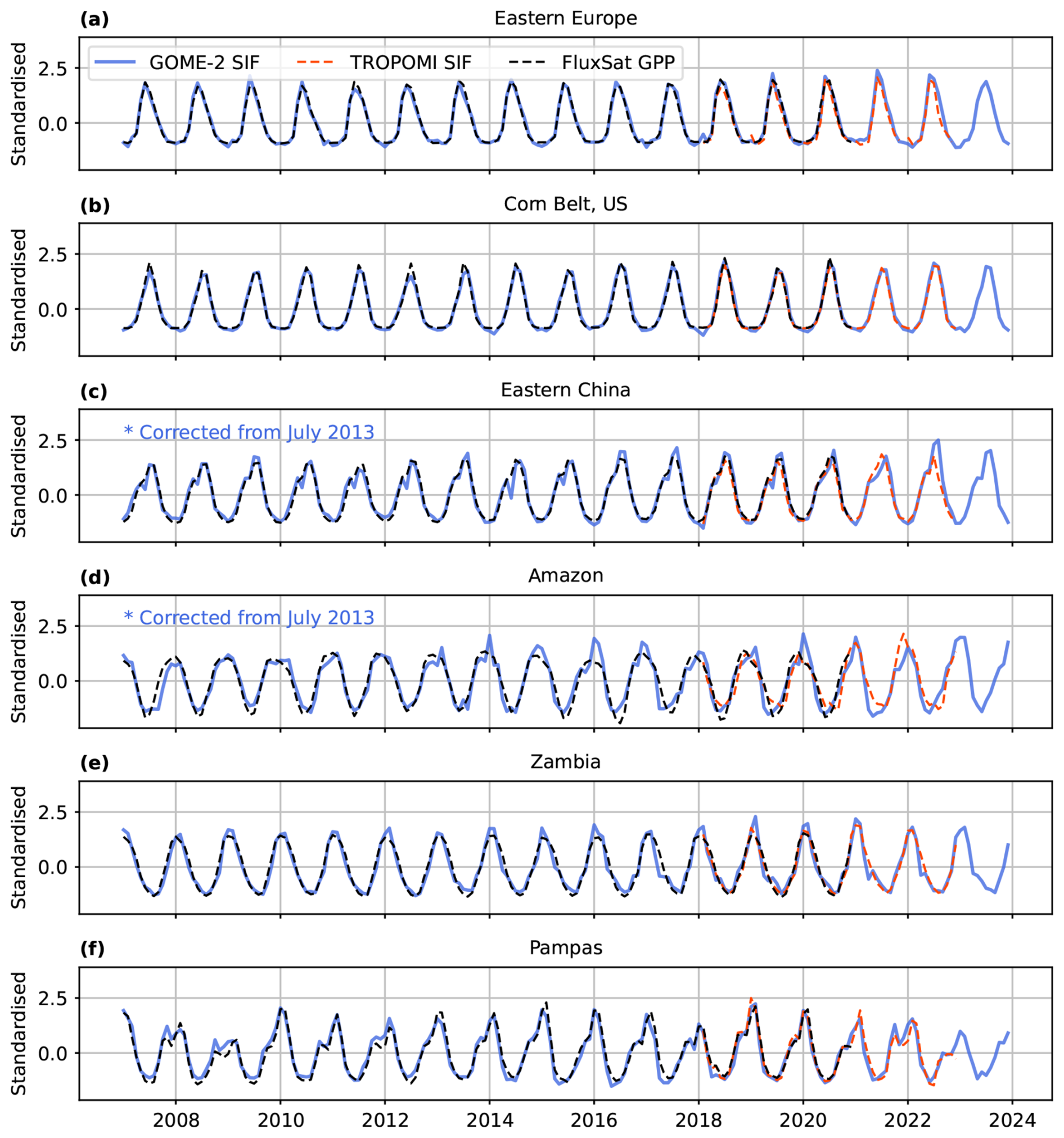
Figure 13 Time series of standardized SIF retrieved from GOME-2 (solid blue), FluxSat GPP (dashed black) and TROPOMI SIF (dashed orange). Since the GOME-2 dataset covers the entire FluxSat GPP period, it is standardised based on the same timespan (January 2007–December 2020). This enhances the alignment of GOME-2 SIF and FluxSat GPP. The used FluxSat data reflects daily averaged GPP.

GOME-2 SIF also agreed strongly with TROPOMI SIF (January 2018 to December 2022), with r=0.86 over the Amazon and r≥ 0.95 elsewhere. In Eastern China, GOME-2 SIF often reveals an early-season peak, which FluxSat GPP does not capture. This feature is also present in TROPOMI SIF (e.g., in 2022), suggesting that SIF is sensitive to subtle phenological features not reflected in reflectance-based GPP.

When evaluated separately, e.g. in Zambia, GOME-2A SIF generally demonstrates slightly higher correlations with FluxSat GPP (r=0.98) than GOME-2B SIF (r=0.94), resulting in an overall lower correlation for the combined record (r=0.96). While these analyses are based on different periods and should therefore be interpreted with caution, they suggest enhanced robustness within the GOME-2A SIF record. This is consistent with larger uncertainty within GOME-2B SIF as compared to GOME-2A SIF (Fig. 6). Nevertheless, GOME-2B SIF maintains strong correlations with both FluxSat GPP and TROPOMI SIF, indicating that the underlying signals remain sufficiently robust.

Overall, these results indicate that the combined GOME-2 SIF record does not exhibit temporal biases or inconsistencies, including false trends induced by instrumental artifacts. Together with the findings by Anema et al. (2025a), this confirms the effectiveness of the advanced degradation correction applied by SIFTER v3 to enable robust and temporally consistent SIF records from both GOME-2A and GOME-2B SIF. When small intersensor offsets are present, our framework in Sect. 5.1 has proven effective in resolving these biases and enabling GOME-2A and GOME-2B to be treated as one long-term dataset for monitoring vegetation activity.

6 Code and data availability

The GOME-2A SIF data used in this work are publicly available under data doi https://doi.org/10.21944/gome2a-sifter-v3-solar-induced-fluorescence (Anema et al., 2025a). The GOME-2B SIF data obtained and used in this work can be accessed at https://doi.org/10.21944/gome2b-sifter-v3-solar-induced-fluorescence (Anema et al., 2025b). The GOME-2 SIF data are provided by KNMI within the framework of the EUMETSAT Satellite Application Facility on Atmospheric Composition Monitoring (AC SAF). The code to detect and correct for intersensor offset biases within GOME-2 timeseries is available on request.

7 Conclusions and outlook

We presented a combined GOME-2 SIF dataset spanning from 2007 to 2023, which combines SIF observations retrieved from both GOME-2A and GOME-2B. The GOME-2A SIF record (2007–2017) was previously retrieved using the SIFTER v3 retrieval algorithm (Anema et al., 2025a). Here, we extended this dataset by applying the same algorithm to GOME-2B data from 2013 to 2023. SIFTER v3 incorporates an advanced correction that addresses time, wavelength, and scan-angle dependencies of reflectance degradation – resolving temporal inconsistency issues.

Although GOME-2A and GOME-2B are identical in sensor design, they are affected differently by instrumental artefacts. We showed that, if not properly corrected for, these differences can induce intersensor biases. During the overlapping tandem phase, seasonally averaged SIF values from both sensors agreed within 2.1 % when co-sampled across time, space, as well as viewing geometry. In contrast, failing to address differences in viewing zenith angle (VZA) sampling can introduce biases in GOME-2B SIF of up to 15 % over high SIF regions. This discrepancy mainly arises from intersensor differences in captured VZA ranges, due to the reduced swath mode of GOME-2A.

Statistical analysis revealed no significant step change at the transition from GOME-2A to GOME-2B in mid-2013 for most case studies; however, it detected small offsets in Eastern China and the Amazon. Applying an additive intersensor offset correction in these regions enhanced the temporal coherence of the GOME-2 record and increased its correlation with independent FluxSat GPP. In the Amazon, the correction reduced the absolute SIF − GPP difference across the sensor transition by more than 20 %. Finally, we demonstrated strong coherence between the GOME-2 SIF record and FluxSat GPP (r≥ 0.92), as well as between GOME-2 SIF and TROPOMI SIF (r≥ 0.87) across regions with different biomes – supporting its use for long-term monitoring of vegetation activity. Our methodology provides a framework to detect and, when necessary, correct for intersensor-related offsets, enabling the use of GOME-2A and GOME-2B SIF as a one coherent record.

Beyond the use of GOME-2 SIF for long-term monitoring, this study offers practical guidance for harmonising multi-sensor datasets. First, achieving internal consistency within each record is essential before merging. Second, differences in viewing geometry sampling can substantially bias intersensor observations and should be addressed, particularly for wide-swath instruments. Finally, the presented framework could be applied to identify and correct for structural breaks in other multi-sensor records. These insights will be valuable for extending the GOME-2 record with GOME-2C observations and for preparing to combine future SIF observations from Sentinel-5 aboard the upcoming Metop Second Generation A series (Metop-SG-A) satellites, for which SIF retrievals are expected to be technically feasible.