Regional Oceanographic Database (BaRDO) for the Argentine Continental Shelf

The Regional Oceanographic Data Base (BaRDO) contains 25 845 quality-controlled oceanographic stations acquired by INIDEP research vessels in the Southwest Atlantic. This paper describes the operability of the data management system, the characteristics and accuracy of the dataset, the quality-control procedures, and the main errors detected and corrected during the flagging process. In addition, we present information on the geographical and temporal distribution of the data, the evolution of the dataset in response to technological advances, and recommendations for its use.

BaRDO contains two main data types: quasi-continuous CTD profiles (conductivity, temperature, and depth) and discrete, low-resolution OSD (Ocean Station Data) profiles. The majority of observations comprise temperature and salinity, while fluorometry, oxygen, and turbidity are also available when measured. Cruise listings and data access covering the period up to 2012 are provided at https://catalogo.inidep.edu.ar/geonetwork/ (last access: 13 July 2026; https://doi.org/10.47193/bottle.temp-sal.1969-2012.v1, Baldoni, 2026a; https://doi.org/10.47193/ctd.inidep.1984-2012.v1, Baldoni, 2026b).

1 Introduction

In the Southwest Atlantic, the total extension of the Argentine Continental Margin – comprising the continental shelf, slope, and rise, as well as the Malvinas Plateau and the Scotia Arc – covers an area of around 2×10⁶ km² (Violante et al., 2014). This extent was significantly increased after the 2017 recognition of the outer limits of the Argentine continental shelf, which added approximately 1.7×10⁶ km² beyond 200 nautical miles (COPLA, 2017).

The Argentine Continental Shelf (ACS) is one of the world's largest, spanning about 9.6×10⁵ km². It extends north–south for about 2400 km, from the Río de la Plata (35°30^′ S) to Cape Horn (57° S), with an average width of 400 km.

The area is a highly productive marine ecosystem (Acha et al., 2004, 2018; Lutz et al., 2010; Diaz et al., 2018; Gil et al., 2019; Cepeda et al., 2024) and plays an important role in the regional heat and global carbon cycle (Bianchi et al., 2005, 2009; Kahl et al., 2017). A variety of fishery resources of economic significance (Villasante et al., 2015; Marrari et al., 2013; Alemany et al., 2009, 2021; Bogazzi et al., 2005) are primarily located along the coastal sector of the ACS, from the mouth of the Rio de La Plata (34° S) to the southern tip of South America (55° S), including the Argentine–Uruguayan Common Fishing Zone (ZCP, between 34–39°30^′ S).

Oceanographic surveys in the Southwest Atlantic began in the early 20th century with the German Antarctic expedition aboard R/V Deutschland (1911–1912), which operated in the Brazil–Malvinas Confluence región (around 38° S off the continental shelf, Schmid and Garzoli, 2009). Subsequent missions by R/V Meteor expedition (1925–1927), R/V W. Scoresby (1927–1932), and R/V Discovery I and II (1931–1936) made significant contributions to the oceanographic understanding of the ACS.

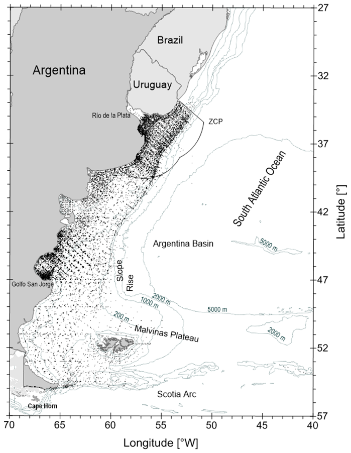
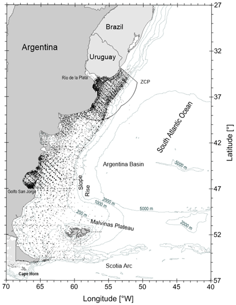
Figure 1 Geographical distribution of BaRDO stations carried out by INIDEP (ZCP: Argentine–Uruguayan Common Fishing Zone).

In the 1960s, the Argentine government, in cooperation with the United Nations Development Programme (UNDP) and the Food and Agriculture Organization (FAO), launched the Fishery Development Project. This initiative included eleven cruises under the Pesquerías program (1966–1969) (PDP, 1971). The research developed as part of this project provided relevant data that contributed to a better understanding of the Argentine Sea's fishery resources, including their spatiotemporal distribution, bioproductive capacity, and economic potential.

In 1977, the routine evaluations of fishery resources in the ACS were initiated, following the establishment of the National Institute for Fisheries Research and Development (INIDEP) and the signing of international cooperation agreements with Japan (Japan Marine Fishery Resource Research Center – JAMARC) and Germany (Federal Research Center for Fisheries – BFAFi). The first cruises under this collaboration were carried out in 1978 aboard the R/V Walter Herwig (Germany) (Ciechomski et al., 1979) and R/V ShinkaiMaru (Japan) (Cousseau et al., 1979).

With the acquisition of its own research vessels – R/V Dr. Eduardo Holmberg (Japan, 1980), R/V Cap. Oca Balda (Germany, 1983), and the adaptation of a coastal fishing vessel later renamed R/V Capitán Cánepa (1979) – INIDEP began regular sampling of oceanographic variables, primarily associated with fisheries research. More recently, INIDEP acquired two modern fisheries and oceanographic vessels: R/V Víctor Angelescu in 2017 and R/V Mar Argentino in 2020, both designed and built to comply with rigorous technical standards.

Over the past 47 years, continuous operations of INIDEP research vessels have constituted the primary source of physical oceanographic data for the region. The spatial distribution of the stations (Fig. 1) illustrates the scope of this effort and the extensive coverage achieved across the Argentine Continental Shelf (ACS).

In 2005, the INIDEP Physical Oceanography group, with support from the Global Environment Facility (GEF) Patagonia Program, began developing an oceanographic database to provide a complete quality-controlled physical dataset of the Southwest Atlantic with special focus on the ACS region. The creation of the Base Regional de Datos Oceanográficos (BaRDO – Regional Oceanographic DataBase) enabled the development of improved temperature and salinity climatologies (Baldoni et al., 2015) and provide a baseline information for oceanographic and ecosystem studies (Simionato et al., 2010; Delgado et al., 2014; Lomovasky et al., 2011; Kahl et al., 2017; Palma et al., 2020; Pisoni et al., 2020; Risoli et al., 2020; Temperoni et al., 2020; Temperoni et al., 2021;).

Even though BaRDO incorporates external data from public databases and individual researchers, this work specifically describes the data structure and management system of the oceanographic stations exclusively collected by INIDEP between 1981 and 2024.

2 Data origin

At the time of submitting this paper, BaRDO holds and manages 25 845 quality-controlled oceanographic stations from 872 research cruises. Most (93 %) of the stations were carried out onboard INIDEP R/Vs, while the rest were developed on small ships or fishing vessels, and a small proportion (less than 2 %) were measured from the coast. The database comprises two distinct types of data: 93 % of the stations were collected using quasi-continuous CTD profilers, the remaining 7 % comes from discrete water sample observations (OSD), primarily acquired before 1993. The annual distribution of oceanographic stations, by type of instrument – OSD, CTD – is shown in Fig. 2. Data collected before 1999 were incorporated into the World Ocean Database (WOD-accession numbers 0089784, 0020559, 0115150, and 0143331) (Mishonov et al., 2024).

Figure 2 Number of yearly stations stored in BaRDO.

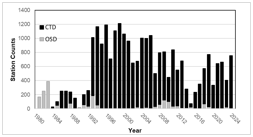
During the first few years, all measurements correspond to OSD profiles; the first CTD was acquired in 1984, and with the incorporation of new equipment from 1993 onwards, the average number of stations per year increased from 193–981 until 2006. Since 2007, the average number of stations per year has been around 540, with a period of low activity between 2014 and 2017, during which the annual average dropped to 237 stations.

Approximately 80 % of the stations were conducted in shallow waters (<200 m depth), with temperature and salinity measurements available in 98.5 % and 97.4 % of cases, respectively. Additional parameters such as fluorometry (32 %), oxygen (2.4 %), and turbidity (6 %) were recorded at a smaller subset of stations.

2.1 OSD

The first measurements of physical variables were carried out in 1981 using Knudsen inversion bottles and initially constituted the only source of temperature and salinity data for fisheries studies. Temperature was measured with reversing thermometers, and salinity was determined using laboratory salinometers. However, there is a lack of information on the specific salinometers used and on the algorithms and standards used for salinity determination.

In 1984, with the deployment of the first CTD, bottle sampling became an alternative used only when the CTD was unavailable; consequently, the annual percentage of OSD profiles decreased significantly (Fig. 2) with a maximum of 187 stations in 1993. From 1984 onward, sampling was conducted using Niskin-type bottles, and salinity determinations were performed in the laboratory using Beckman and Tsurumi-Seiki salinometers between 1987 and 1994, applying different salinity algorithms and non-systematic use of seawater standards. Since then, a Guildline Autosal 8400B salinometer (accuracy ±0.003 PSU; precision 0.0003 PSU), calibrated with IAPSO Standard Seawater (Ocean Scientific International OSIL, P106 to P167), has been used.

2.2 CTD

Until 1993, the only CTD available was the ME Meerestechnik Elektronik instrument. This CTD remained operational until 2010, and the stations sampled with it represent 13 % of the total dataset. Furthermore, between 1993 and 1997, the CTD NBIII-III/V, although not part of INIDEP's equipment, was used in several cruises on loan from the SHN (National Hydrographic Service).

The ME CTD system was gradually phased out as Sea-Bird Electronics (SBE) profilers became the operational standard. INIDEP progressively acquired different CTD models from this manufacturer: SBE 19 in 1993 (SN1268), 1995 (SN1683), 1996 (SN1806), and 2001(SN3030); SBE 911plus (SN09P8073-0359) in 1994 and later in 2017 (SN09P63966-1045); SBE 25 (SN2542135-0412) in 2007; and finally, SBE 25plus (SN1219) in 2021.

Until 2017, water samples for CTD in situ calibration were collected using a Niskin bottle attached to an oceanographic cable and closed by a messenger. Since then, sampling with a rosette system (General Oceanic GO1015; SBE32; SBE55) has been used to improve the collection of water samples at defined depths.

Table 1 Technical characteristics of CTD models.

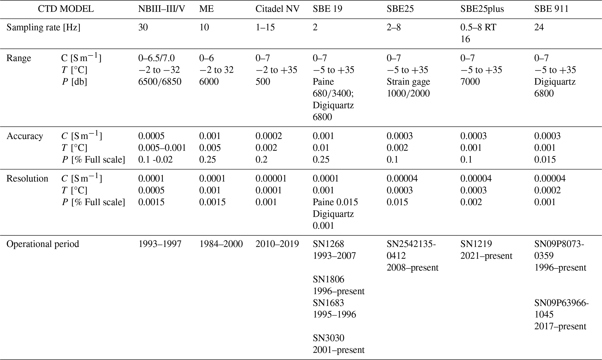
The characteristics of each CTD model used and their operating periods are summarized in Table 1. Figure 3 shows the percentage of oceanographic stations carried out by each CTD model, along with the corresponding proportion of OSD profiles.

Figure 3 Oceanographic data distribution by instrument type and model.

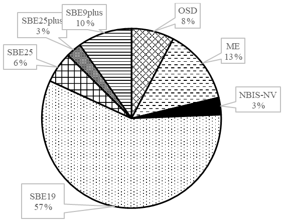
The largest share (57 %) corresponds to the SBE19 model, followed by the ME (13 %), which remained in use until 2000. The data were collected in real-time using a conducting oceanographic cable, except for 20 % of the stations collected with SBE19 profilers and for all measurements from the Citadel NV, which were operated in internal recording mode.

To illustrate differences in the performance of CTD models, Fig. 4 illustrates temperature and salinity profiles recorded by different SBE CTD models under two typical vertical stratification conditions over the ACS during the warm season.

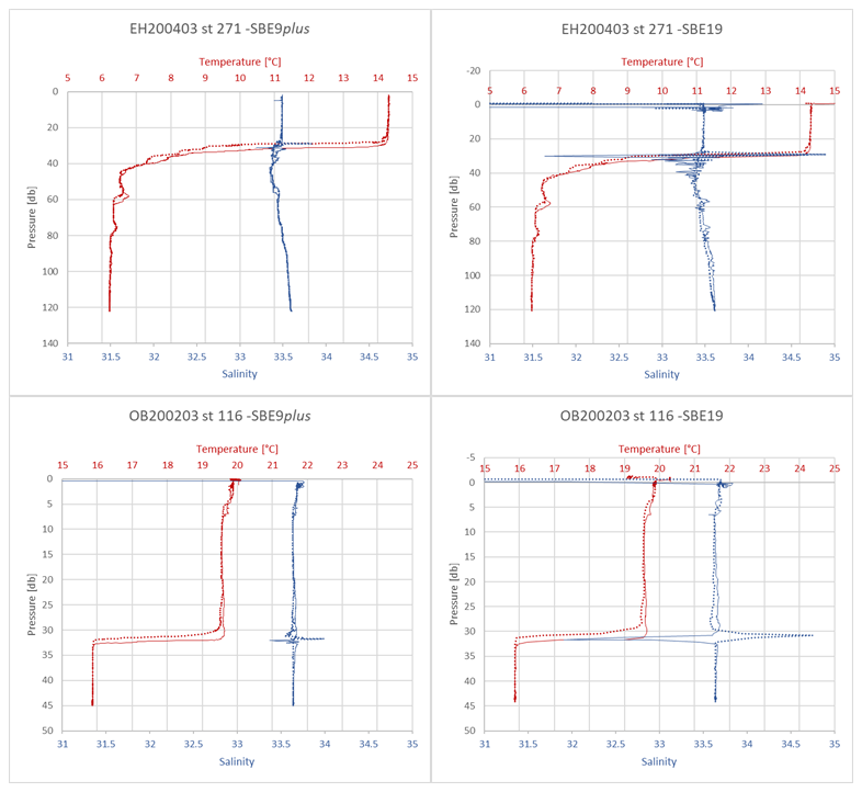
Figure 4 Temperature and salinity profiles versus pressure from different CTD models: SBE19 (left) vs. SBE9plus (right). Solid lines indicate the downcast and dashed lines indicate the upcast.

For SBE19 data, although a pump is employed to minimize sensor response lag, residual mismatches may result in spurious salinity and density signals at the zone of thermal gradient. In contrast, the SBE9 model – with higher sample rates, faster-response sensors, and a Temperature–Conductivity (TC) duct assembly (Seabird Application Note 38) – produces less noisy salinity and density measurements. Some of these differences between CTD models can be resolved through appropriate signal processing; however, a significant number of flagged salinity data points should be expected at the thermocline level under stratification conditions, depending on the instrument used.

Figure 5 Data management system flow diagram.

3 Data management system

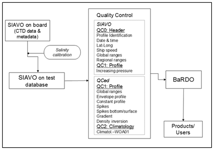
Figure 5 illustrates the flow diagram developed to manage physical data measured onboard INIDEP research vessels, including their acquisition, storage, and availability for user access. The system was developed considering the specific working conditions onboard and its evolution over time. Since 1993, the significant increase in the number of oceanographic stations – associated with the incorporation of new CTDs – has led to a high demand for onboard technical personnel. Initially, this requirement was met by INIDEP-trained staff, although turnover rates were high. At that time, despite the availability of working protocols, the lack of automated storage systems for key variables, including position, bottom depth, and meteorological parameters on INIDEP vessels, together with the participation of many different operators, considerably increased the likelihood of human error. To address this issue, it became necessary to design an automated data acquisition process that incorporated navigation data and provided an organized structure to minimize data entry errors. The objective was to ensure accurate recording and transfer of information, and to enable the application of quality-control procedures for error identification and correction. With this aim, the SIAVO system (Sistema Integral de Almacenamiento de Variables Oceanográficas – Integral System for the Storage of Oceanographic Variables) was developed. SIAVO manages onboard data acquisition, processing, and storage of oceanographic data in an MS Access database. After each cruise, SIAVO exports the onboard database to a staging database for verification and basic quality control of the raw data. Once salinity correction (Sect. 3.2) and station profile quality control procedures (Sect. 3.3) have been completed, the final dataset is stored in BaRDO (Microsoft SQL Server) for further use and distribution to end users.

3.1 Database design and principles

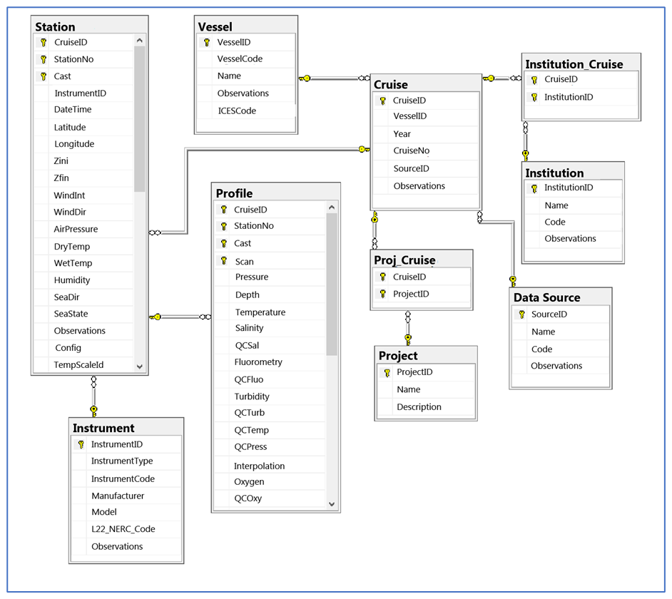
Both SIAVO and BaRDO databases share a similar logical structure, organized around three main tables:

• Cruise: stores general information about each survey (vessel, year, cruise number).

• Station: compiles station-specific information (station number, cast, starting position and UTC date/time, time zone, bottom depth, temperature scale, instrument, and meteorological variables).

• Profile: contains the vertical distribution of the observed variables: temperature, salinity, oxygen, etc. Derived variables (e.g., potential temperature, density, buoyancy, sound velocity) can be computed dynamically by built-in functions based on EOS-80 algorithms (UNESCO, 1981a, b; Fofonoff and Millard, 1983; Millero et al., 1981) integrated into the database for this purpose.

The structure of the database tables enables easy expansion to include new vessels, sampling instruments, and parameters, and facilitates data search with diverse criteria (spatial area, time, ship, project, instrument, etc.).

The general entity-relationship model of BaRDO is shown in Fig. 6. Some of the tables included are: Vessel, Cruise, Instrument, Data Source, Institutions, Project, Station, and Profile. The identification key for each oceanographic station results from the unique field combination of CruiseID + Station number + Cast number; relationships between the cruise, station, and profile tables are one-to-many. Each record in the Cruise table is related by the primary key CruiseID to several records in Station table, which equals to the number of casts in the cruise. Similarly, in the Station table, the composite primary key (CruiseID + Station number + Cast number), becomes a foreign key in the Profile table, where measurement levels for each cast are stored.

Figure 6 Regional Oceanographic Data Base (BaRDO) entity relation model.

3.2 Data processing and calibration

Data acquisition was performed using calibration coefficients from the manufacturer's certificates (static calibration). For fluorescence measurements, a blank reading is taken before each oceanographic cruise, and an offset correction is applied to the data. This section describes the temperature monitoring and the corrections applied to salinity data. Oxygen and turbidity data are reported exclusively using the manufacturer's coefficients.

CTD data were processed using Sea-Bird Data Processing software, available for free at https://seabird.com (last access: 13 July 2026). In the case of non SBE instruments, the data were previously converted to an ASCII format and then incorporated into the standard Sea-Bird Data Processing software steps.

Obtaining accurate salinity estimates from CTD measurements requires extensive processing and multiple corrections to account for sensor response characteristics (McTaggart et al., 2010). The routines and parameters depend on the CTD model, with their final selection determined by factors such as water column stratification, lowering speed, sea state, and the time allowed for surface stabilization. However, in highly stratified waters and depending on the CTD model used, it is not possible to eliminate spikes in the profile, even after adjusting the parameter values in each routine.

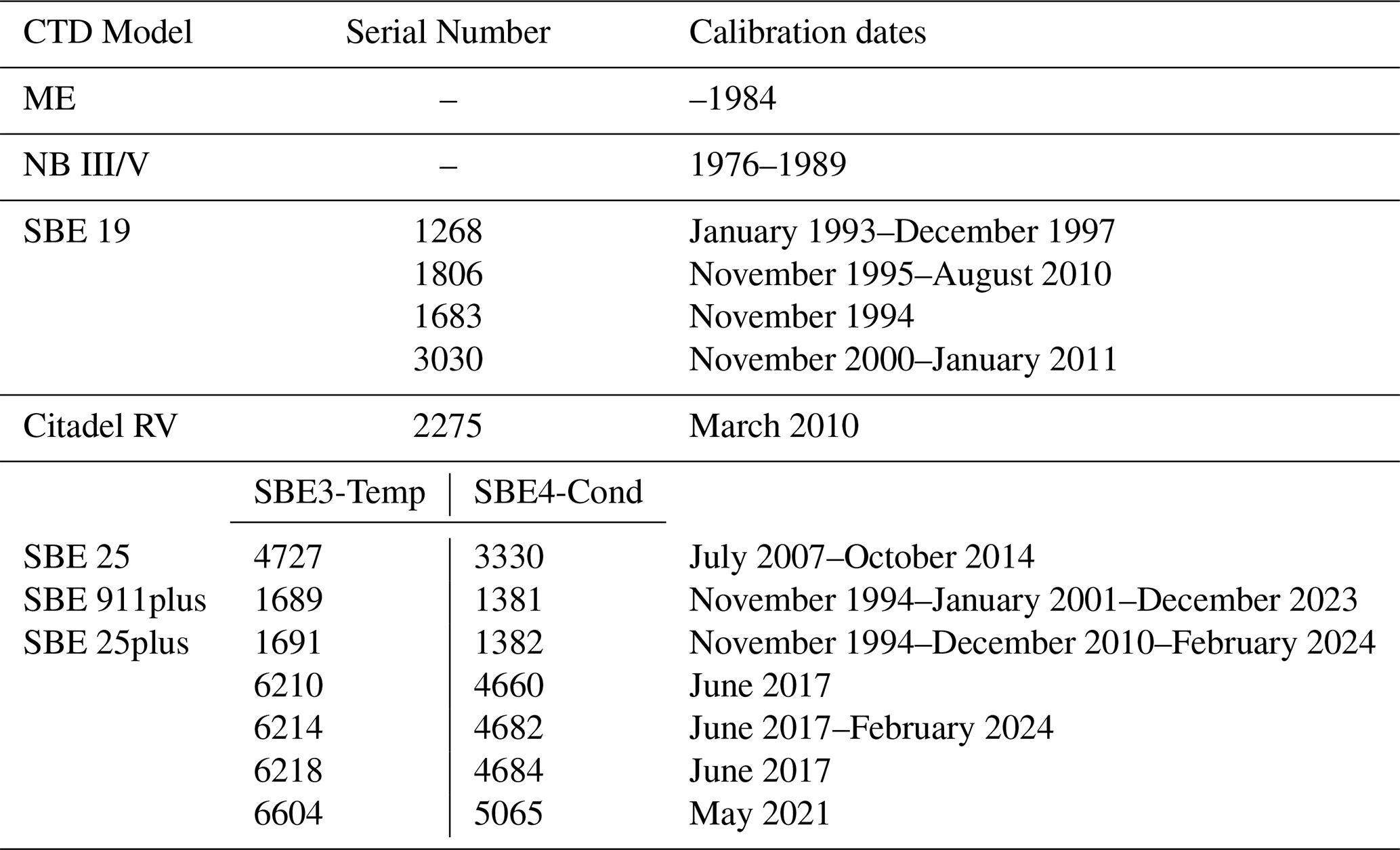
For calibration purposes, it is important to note that manufacturer-provided CTD calibrations were limited, as shown in Table 2, largely due to the cost and bureaucratic challenges associated with temporary exports. Consequently, sensor stability between calibrations has been monitored over time by comparing paired instruments/sensors, paying particular attention to temperature sensors, since no in situ calibrations were applied during processing.

Table 2 Manufacturer calibration dates by instrument.

3.2.1 Temperature

Monitoring of temperature sensors between manufacturer calibrations is shown in box plots of temperature differences in Fig. 7. The boxes represent the interquartile range (Q1–Q3), the solid lines indicate the median, the crosses denote the mean, and the whiskers extend to the minimum and maximum values, excluding outliers.

Until 2017, sampling was carried out using CTDs with a single pair of sensors; therefore, temperature sensor monitoring was only performed when paired instruments were available. These comparisons were made between: ME vs SBE 19 (SN: 1268 and 1806); different SBE 19 s (SN: 1268, 1806, 3030); SBE 911plus (SN: 1689, 1691, 6214) vs. SBE 19 (SN:1268, 1806, 3030) and SBE 25 (SN4727) vs. SBE 19 s (SN: 1806 and 3030) (Fig. 7a). From then on, it was possible to optimize the control for modular sensors mounted as primary and secondary sensors on the same SBE 911plus CTD (SN: 4727, 1689, 1691, 6210, 6214, 6218, and 2230) (Fig. 7b).

It's important to note that, when working in shallow waters (mostly<200 m), even within homogeneous layers, the accuracy of estimated differences is inherently limited due to their high natural variability. In addition, when sensors are mounted on different CTD fish, their relative position on the carousel may introduce further uncertainty. Even taking these factors into account, the maximum temperature differences calculated between distinct instruments remain below ±0.02 °C, whereas comparisons between sensors mounted on the same fish show differences of less than ±0.005 °C.

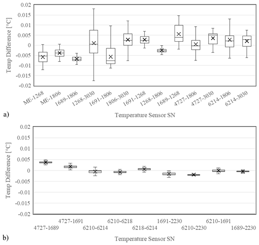
Figure 7 Temperature differences comparisons between different paired CTD models (a) and different sensors mounted in the same SBE 911plus fish (b).

3.2.2 Salinity

In the case of conductivity sensors, instrumental drift represents a more significant problem when CTDs are not regularly calibrated by the manufacturer to ensure stability and accuracy. To mitigate this, strict protocols are followed to keep the conductivity cells clean and uncontaminated, and a systematic salinity sampling program is implemented for subsequent adjustments. Comparisons between bottle-sample salinities and CTD-derived measurements enable the detection and correction of errors due to sensor drift or calibration offsets. Salinity samples for in situ calibration have been collected since 1987, and the methods and instruments used to measure them have evolved (see Sect. 2.1).

These water samples for salinity correction are collected in the most stable part of the water column; however, this condition is not met at all stations. Additionally, given that most measurements are conducted in waters shallower than 200 m, salinity samples are often collected at a single pressure level. Consequently, only a limited number of salinity samples are available per cruise for calibration purposes, and in most cases, a temporal analysis by instrument is performed.

Salinity corrections are based on a linear adjustment using the least squares method. The fitting equation and its basic statistics – correlation coefficient, standard error of the regression, and number of observations- are stored in BaRDO (not shown), along with the type of analysis performed -by cruise or by instrument over a defined period.

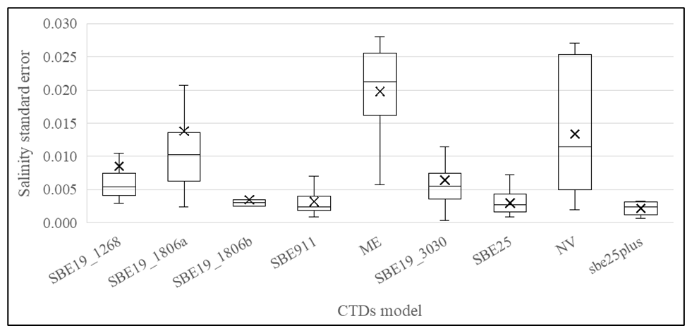
Figure 8 follows the same box-plot format as Fig. 7 and shows regression standard errors by instrument, to assess the accuracy of different CTDs' salinity correction models and inform users about the precision of the reported salinity values.

The lowest regression standard errors are observed for the SBE 911 and SBE 25 CTD models (<0.005). The highest errors are found for the ME CTD, reflecting the limited availability of bottle data for corrections, the use of different salinometers, and the scarcity of calibration standards. For the NV instrument records, the greater dispersion is mainly associated with its use in shallow, low-salinity coastal waters (≈70 % at depths of less than 25 m). Within the SBE19 group, error magnitudes vary among individual instruments. Unit SN1806 exhibits the highest mean error (∼0.01) and the largest standard deviation during the period before 2010 (SBE19_1806a in Fig. 8), whereas after that date (SBE19_1806b in Fig. 8) the values fall below 0.005. This behavior may be explained by the original configuration of this CTD, which included a pack of six batteries and an associated pump that, during some cruises, was replaced by a higher-power pump. This change likely affected pump performance, causing it to operate more slowly or intermittently and thereby degrading data quality. Although it is not possible to determine the exact period during which the instrument operated with the high-consumption pump, since 2010, the CTD has been modified to include a pack of nine batteries, allowing the use of both pump models.

Figure 8 Standard error from salinity regression analysis by instrument.

3.3 Quality-control

Quality-control (QC) procedures described here have been developed in accordance with the IOC (International Oceanographic Commission) recommendations (CEC, 1993; UNESCO-IOC, 2010). QC routines are run on individual stations and cruise groups. The controls are classified as: station data (QC0), profile data (QC1) and climatological comparisons (QC2). The quality-control codes assigned are listed in Table 3.

Table 3 Data quality codes.

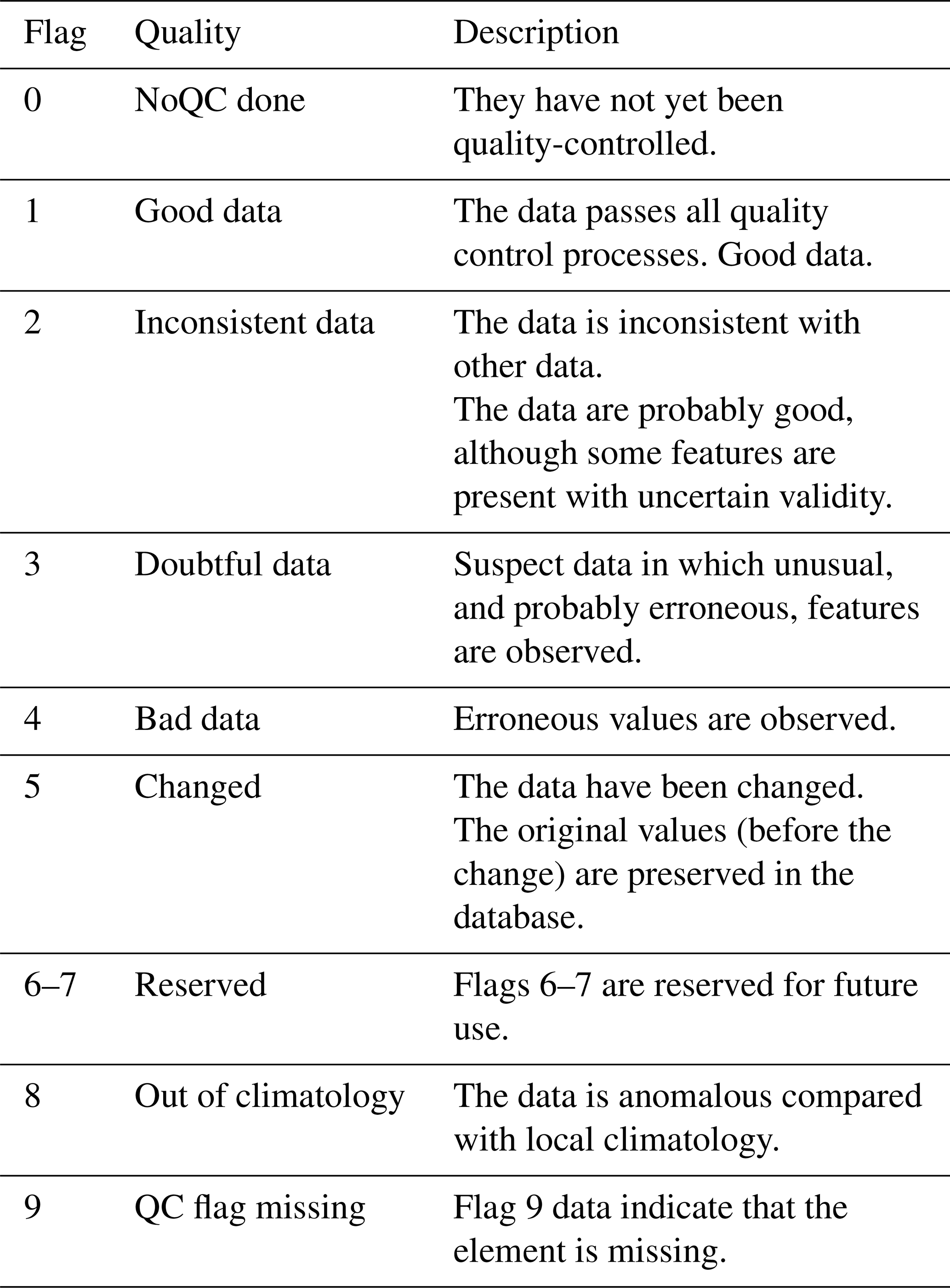
QC0 is performed within the SIAVO environment on station data, verifying both the identification fields (vessel name, cruise number, station number, position, and date/time) and the associated meteorological information. The operator may accept or modify the assigned quality-control flag and correct the data as needed. When a variable is modified, the original value is saved, and the field is marked as “changed” (QC=5), and all quality-control checks associated with the changed field are rerun using the new value. This QC0 level includes routines to check data format, date/time, sequential station numbers, ship' s speed between stations, global and regional ranges (cruise, station, cast number, latitude/longitude, depth, and meteorological data), and the consistency between the bottom depth and the maximum depth of the measurement.

The QC1 and QC2 level control groups are associated with profile observations in each oceanographic station. This task is performed using the Data Quality Cruise Editor (QCEd) software (original version 1.5 – https://www.nodc.noaa.gov/gtspp/software/qced/index.html, last access: 13 July 2026) provided by the Global Temperature-Salinity Profile Program (GTSPP/NODC/NOA).

The program performs a suite of automated data quality tests to detect constant profiles, spikes, gradients, and density inversions when both temperature and salinity are available, or temperature inversions when only temperature is present. It displays “trouble lights” to alert the operator to questionable data. At this stage, only QC flags can be edited; observed temperature or salinity values cannot be modified. Thresholds implemented by QCEd V1.5 are summarized in Table 4, with gradient thresholds expressed in units per dbar.

Table 4 Thresholds of QC routines.

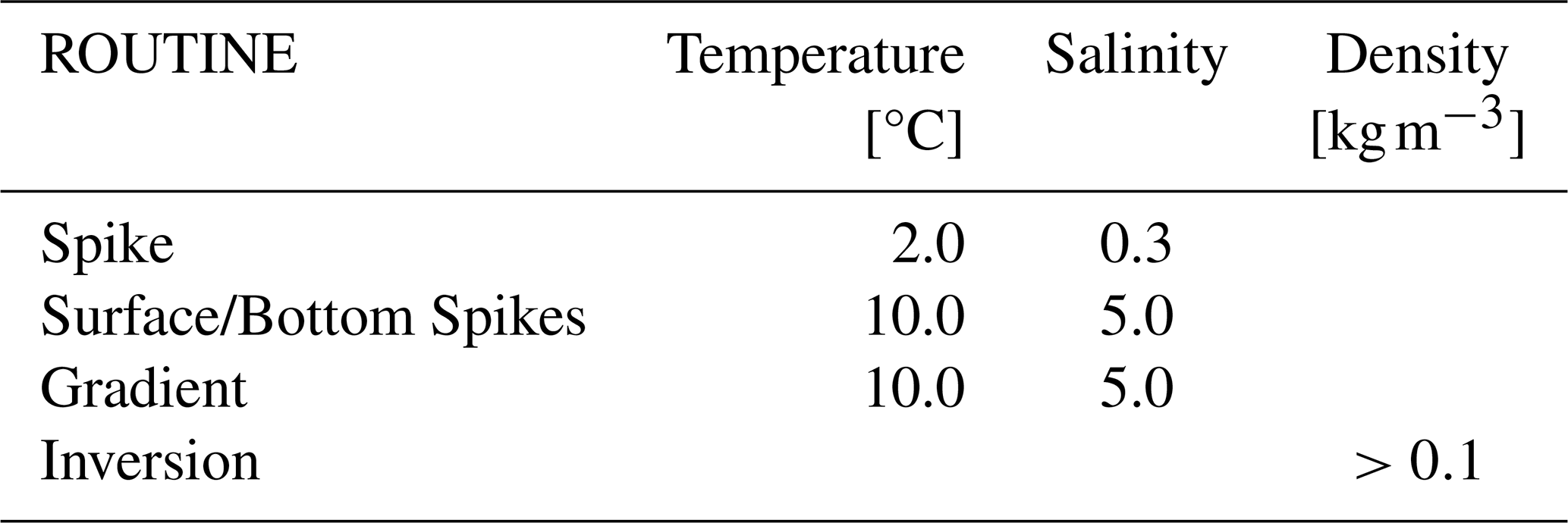
First, automatic quality controls are executed. Then, an analyst conducts a visual examination to validate or manually adjust the flags based on overall data consistency. Regarding modifications to automatic flagging, it is important to note that if data pass the thresholds set by automatic control, no changes are made. The original flag is retained even when analysts may consider the data suspicious. When in doubt, analysts adopt this conservative approach to avoid incorrectly flagging good data as suspicious. This protocol minimizes subjective flagging, ensuring uniform criteria consistent with the current thresholds across the entire dataset.

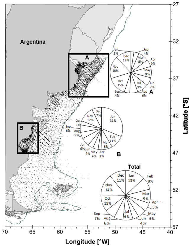
Figure 9 Geographical and monthly distribution of BaRDO stations.

4 Results

4.1 Spatial and temporal coverage of the database

In Fig. 9, the geographical coverage of INIDEP oceanographic stations displays a sampling strategy directly linked to the evaluation of specific fishery resources. The observational effort is focused on the continental shelf, within the 200 m isobath. Most stations are located in the Argentine–Uruguayan Common Fishing Zone (box A) and the San Jorge Gulf (box B), which together account for 64 % of the stations in the database. Data from latitudes south of 47° S were especially sparse. Temporal coverage of data – inside graphs – was also uneven, as sampling was related to the months of stock evaluation mainly for red shrimp (Pleoticusmuelleri) and Argentine hake (Merluccius hubbsi). Both species are monitored in box B in January, while from October–December, the hake hubbsi biomass is estimated in box A. Overall, the temporal distribution of total dataset across the ACS (Fig. 9, bottom right-hand corner) is relatively homogeneous, with higher coverage percentages in November and January, while June and April are somewhat less well sampled.

4.2 Results of the quality control

Stations flagged as inconsistent, doubtful, or poor-quality represent less than 6 % of the total. This condition is primarily influenced by the instrument type, time of year, sampling region (stratified or non-stratified profiles), and water-column depth.

The flagged levels represent only 0.07 % of the total number of temperature observations and 0.31 % of salinity observations.

Figure 10 shows, for each month, the percentage of total sampled levels relative to the complete dataset (black dots), together with the percentage of flagged temperature and salinity levels relative to the total number of observations in that month. The highest proportion of flagged levels relative to the total number of observations occurs in February and November, mainly in temperature in November and in salinity in February. On the other hand, during the cold months (June–October), when vertical stratification substantially decreases, the percentage of flagged levels relative to the total number of observations is considerably lower than during the warm months.

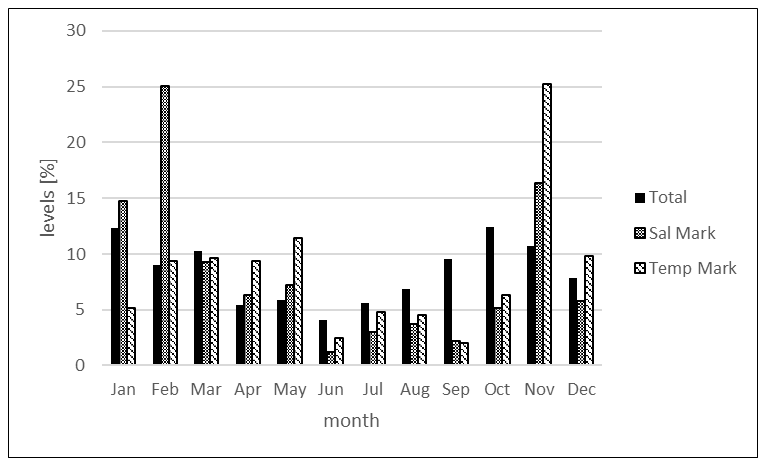
Figure 10 Monthly percentage of sampled data and proportion of flagged ones within each month.

Figure 11 Quality control flags in a stratified profile.

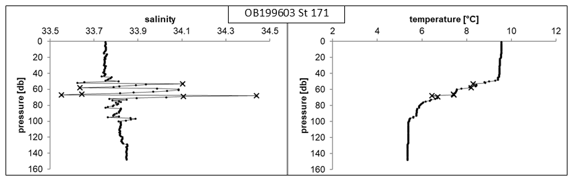
Considering the different instruments, the highest proportion of flagged levels is associated with the SBE 19, which accounts for 57 % of the stations (Fig. 3) and 75.1 % of all flagged levels. In contrast, the SBE 9plus, which represents 10 % of the stations (Fig. 3), accounts for only 6.6 % of the flagged levels. To illustrate the types of flags present in the dataset, Fig. 11 shows typical stratified profiles over the continental shelf, with flagged points (crosses) identified during the quality-control. The spiky salinity is to be expected across these intense thermoclines, and it will be considered that not all the suspicious data has been marked with the established thresholds. In the case of climatological tests (QC2 level), comparison with global climatology (Locarnini et al., 2006; Antonov et al., 2006) does not yield reliable results for the region due to the limited number of observations used in its development. Therefore, based on knowledge of the local distribution of properties, most automatic “inconsistent” flags were discarded.

5 Data availability

The dataset covering the period up to 2012 is published through the institutional GeoNetwork catalogue maintained by the Instituto Nacional de Investigación y Desarrollo Pesquero (INIDEP). The CTD dataset is openly accessible at https://doi.org/10.47193/ctd.inidep.1984-2012.v1 (Baldoni, 2026b), and the discrete water sample observations are available at https://doi.org/10.47193/bottle.temp-sal.1969-2012.v1 (Baldoni, 2026a). The DOIs resolve to the exact versions of the datasets used in this publication. Both datasets are provided in CSV format under the Creative Commons Attribution 4.0 International (CC BY 4.0) license.

Work is currently ongoing to publish the extended dataset covering the period up to 2020. Data from the most recent five years are currently subject to restricted access.

6 Summary and perspectives

This paper introduces the physical oceanographic dataset collected by INIDEP over the past 47 years. The organization of these data within BaRDO, an updated database, has improved accessibility and facilitated the use of ACS data, a region of high environmental, biogeochemical, and economic significance. This resource has already supported numerous scientific studies and is expected to advance understanding of the physical and biogeochemical variability of this marine environment. All data records include an associated quality flag. It should be noted that, in the thermocline, some salinity spikes and density inversions may remain unflagged due to the thresholds applied. To identify all potentially doubtful values, a new dataset version could be generated using more stringent thresholds (e.g., density $\text{inversions}<-\mathrm{0.01}\mathrm{kg}{\mathrm{m}}^{-\mathrm{3}}$ and salinity spikes of 0.03). The development of a new regional climatology incorporating the present dataset would improve future quality-control procedures by providing more reliable reference fields for assessing temporal and spatial consistency at annual, seasonal, and monthly scales.

It should also be noted that the lack of regular CTD calibration under controlled conditions may affect overall data accuracy, particularly given the challenges of conducting field calibration in shallow, highly variable waters. This limitation is partially mitigated by careful cleaning and maintenance of the instruments, complemented by rigorous adjustment using water samples. Following delayed-mode corrections and checks, the accuracy of salinity is estimated at approximately 0.03, while temperature measurements, based on paired instruments, achieve accuracies better than 0.01–0.005 °C depending on the CTD model.