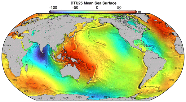
The DTU25 mean sea surface: from and for SWOT

We introduce a new Mean Sea Surface model (MSS) that incorporates the wide-swath altimetry obtained from the Surface Water and Ocean Topography (SWOT) satellite, along with long timeseries of conventional altimetry. The DTU25MSS constrains long wavelengths (>20 km) from a suite of conventional altimeters while utilizing almost 2 years of SWOT observations to reduce the short wavelength noise and incorporate previously unmapped geodetic features into the MSS. Parametric long wavelength corrections of the SWOT data in order to compensate for the short time-scale is presented, and the resulting MSS model is compared with contemporary MSS models as well as data from the SWOT Cal/Val orbit. The MSS is available on https://doi.org/10.11583/DTU.29412275 (Andersen and Nilsson, 2025), and includes an experimental MSS which has the reference period moved to 2023 as opposed to 2003, to compensate for sea level rise. To extend the MSS into the coastal zone, the high-resolution 250 m SWOT data is used close to the coast (<40 km), and resolves complex features previously not included. Using an updated MSS with better resolved short wavelength signals is seen to be a large benefit for interpreting the detailed SWOT observations with reduced leakage of geodetic features into the oceanographic signals, as well as  30 % increase in spatial resolution. Due to incorporating complex novel features in the coastal zone that have been resolved by SWOT the full effect on other more coarse observations is a potential for further studies. The SWOT data and utilization of it is only expected to be improved with time and further development of methods for utilizing this new dataset will move it closer to its full potentials.

1 Introduction

Satellite altimetry has been used to obtain accurate observations of the ocean topography for more than 30 years (Fu and Cazenave, 2001; Rodriguez et al., 2017; Abdalla et al., 2021), where instantaneous ocean topography is time dependent and lies close to the static Mean Sea Surface (MSS). The studies of ocean dynamics therefore primarily utilizes the Sea Level Anomaly (SLA), where the MSS has been removed from the altimetry observations (Stammer and Cazenave, 2018). However, in case of unresolved signal in the MSS, these will still be present in the SLA as noise. Even with 30 years of altimetry available to continuously improve the MSS (Yuan et al., 2023; Schaeffer et al., 2023; Andersen et al., 2023; Laloue et al., 2025). The MSS is still one of the larger sources of error currently in satellite altimetry (Pujol et al., 2018; Dibarboure and Pujol, 2021).

Wide-swath altimetry by the Surface Water and Ocean Topography (SWOT) satellite, launched in 2022, can resolve submesoscale features (Fu et al., 2024; Archer et al., 2025). Many of these short wavelength features show the incredible resolution of SWOT, such as swells (Ardhuin et al., 2024), internal waves (Qiu et al., 2024), directional wave heights (Bohe et al., 2025), eddies (Zhang et al., 2025), ocean vorticity (Carli et al., 2024), ocean tides (Hart-Davis et al., 2024; Monahan et al., 2025; Arildsen et al., 2025) and marine gravity fields (Chen et al., 2025; Tu et al., 2025; Zhu et al., 2025; Yu et al., 2024a). With the oceanographic community focusing increasingly on small scale features, the importance of the MSS reference surface has only increased (Dibarboure and Pujol, 2021).

Incorporating these high resolution observations from SWOT to improve the MSS reference is expected to improve both (a) the quality and interpretability of SWOT data itself and (b) the quality of the 30 year altimetry record, by removing unresolved features. The current state-of-the-art MSS is the 2023 Hybrid MSS, created in preparation for the SWOT mission by combining the latest models CNES_CLS22MSS (here CLS22MSS), SIO22MSS, and DTU21MSS (Laloue et al., 2025). However, this solution still relies on the conventional nadir satellite altimeters, limited by the spatial resolution of these. Initial studies of the SWOT data have shown that the static ocean surface is mapped to a higher precision (Yu et al., 2024b; Nilsson et al., 2025) after only a year of observations, compared with 30 years of nadir altimetry, illustrating the opportunity of utilizing SWOT for MSS mapping.

We present our best effort of utilizing two years of SWOT wide-swath altimetry to construct a global MSS reference field, at $\mathrm{1}/\mathrm{100}$° spacing (∼1.1 km at the equator) in both longitude λ and latitude ϕ, benefiting the intermediate and short wavelengths (<50 km) of the MSS. Section 2 gives an overview of the creation of the model, with a special focus on the processing done in order to utilize the high-resolution data from SWOT. Section 3 presents the model, especially new features discernible in the short wavelengths, with validation and current limitations presented in Sects. 4 and 5.

2 Three stage model creation

The goal of MSS modeling is to obtain the most accurate separation of the mean and time-varying field, given the limitations of the observations and the limited spatial and temporal resolution of each dataset. The model is built up in a remove-restore fashion, where we utilize the observations from the different satellite altimeters optimally (illustrated in Fig. 1). In order to optimally use the high resolution but short temporal scale of SWOT, we build an interim DTU25_LMMSS model based on nadir altimetry, to get as good an averaging over 20 years as possible. The three stages are defined as below, where the wavelengths are indications of the resolution for the nadir altimetry, SWOT as well as the distance from the coast where we utilize SWOT.

• Long Wavelengths: The first stage is to derive the DTU25_LMMSS model using almost all nadir altimetry available during a 20 year timespan. Exact repeat missions (ERM) are used to determine the longest wavelengths, and geodetic missions (GM) are used to resolve wavelengths between 20–200 km. DTU25_LMMSS differs from its predecessor DTU21MSS in accounting for slope correction from conventional altimetry.

• Short Wavelengths: The second stage uses the DTU25_LMMSS model in a remove-restore fashion to resolve shorter wavelengths using the SWOT ocean product (2 km grid spacing). Although SWOT has unprecedented spatial resolution, the short time scale can cause mesoscale features to be captured and transferred to an MSS. We therefore fix all wavelengths of SWOT longer than 50 km to be matching those of DTU25_LMMSS whereby we fix the reference time-period to that of DTU25_LMMSS and also removing most of the mesoscale oceanographic features that are not averaged out from the SWOT observations. This creates the DTU25_2 kmMSS model.

• Coastal Zone: The third and last stage benefits the coastal part in the MSS. The DTU25_2 kmMSS is now used in remove-restore to introduce the SWOT 250 m data in the coastal zones (<40 km from coasts). This enables us to go from 𝒪(5 km) distance from the coast to 𝒪(500 m). The 250 m data are more noisy than the 2 km data, and we therefore aim to use this only in the regime where it will benefit the MSS resolution. When completed in the coastal zone, we add back the longer wavelength features, to get the DTU25MSS.

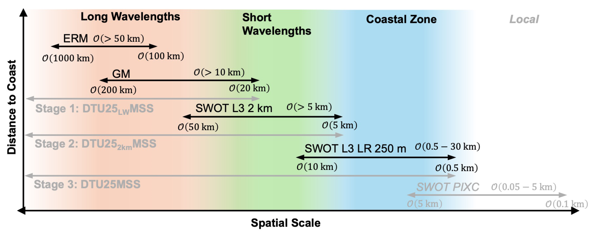
Figure 1 Diagram illustrating the different wavelength regimes refereed in the paper, with the used data for each regime. The three stages are shown with each interim Mean Sea Surface (MSS) model indicated. The last local step is not performed in this paper, but illustrates the possibility for future inclusion of the pixel-cloud data product.

The potential for even smaller scale could be achievable with the pixel cloud data available from SWOT. This would expand the MSS into smaller fjords, complex river outlets and obtain better estimates in the regions with ice cover but would require substantially increased computational resources. This is currently not incorporated into the DTU25MSS.

2.1 Stage 1: long wavelength

2.1.1 The DTU25_LWMSS

The long wavelength part of the MSS is derived along the highly accurate nearly uninterrupted mean profiles of the Exact Repeat Missions (ERM) derived using TOPEX/Jason-1/Jason-2 observations (T/P reference). This reference mission is indicated in Table 1, along with the rest of the satellites and orbital configurations included in the MSS. This is done in a similar fashion as the DTU21MSS (Andersen et al., 2023). where ERM (other than the T/P orbit) and GM missions have been fitted to the 20 year T/P reference period by using the T/P reference as the constraint. This is similar to other MSS methods, utilizing a reference orbit and then fitting other ERM and GM missions to fill the gaps (Andersen and Knudsen, 2009; Schaeffer et al., 2023) At each ground track location we determine a 4 parameter solution to account for the mean and largest time-variable signals using the following equation:

$$\begin{array}{}\text{(1)}& {\displaystyle }\mathrm{\text{SSH}}=\text{MSS}+a(t-t_{\mathrm{0}})+b\cos {\mathit{\omega }}_a(t-t_{\mathrm{0}})+c\sin {\mathit{\omega }}_a(t-t_{\mathrm{0}}),\end{array}$$

where a is the sea level trend and b and c are the coefficients of the in-phase and in-quadrature of the annual signal. In order to ensure that the MSS is determined wrt. to certain mean period the t₀ is fixed to 1 January 2003, the center of the T/P reference orbit (Andersen and Knudsen, 2009; Andersen et al., 2023). To ensure later stages benefits most from the novel SWOT data at short wavelengths, a low-pass gaussian filter with 0.5-gain at 10 km full wavelength has been applied to low and mid latitudes (<70°).

Table 1 Overview of the satellites or orbits used for creation of either the long wavelength MSS or with SWOT. The satellites on the same row are in the same orbit. The TOPEX/Poseidon+Jason-1+Jason-2 orbit (bold) is used as the reference orbit, with a center in 1 January 2003.

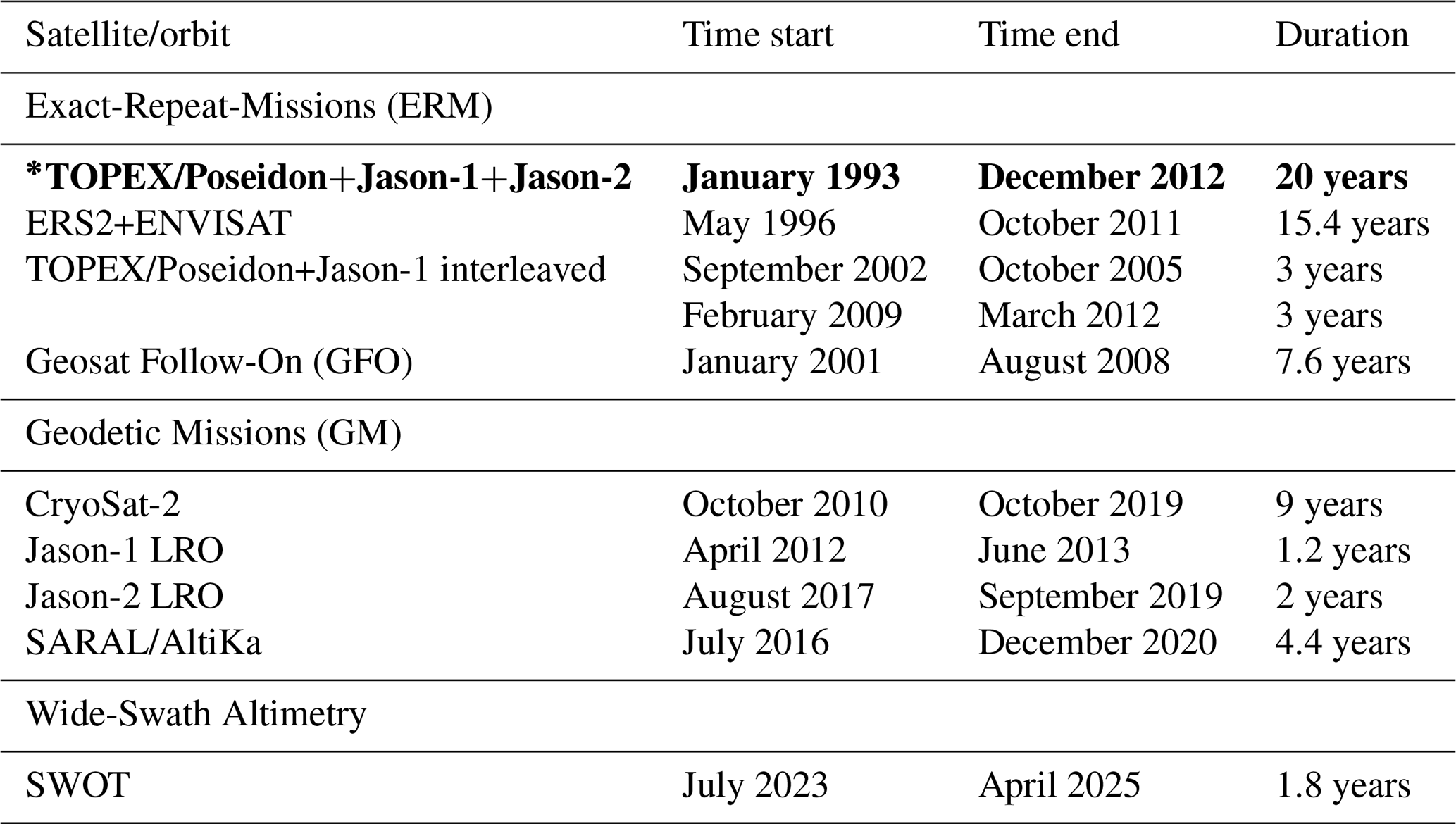
^* Reference mission for MSS.

Over steep geoid gradients it is important to account for the fact that the point of closest approach affecting the sea level observations are not at nadir but up to a few km off-nadir. The corrections was developed by Sandwell and Smith (2014) and ranges up to nearly 40 mm across the Aleutian trench in the northern Pacific Ocean. The correction is dependent on the altitude of the satellite and and is applied to the LRM satellite data as suggested in Sandwell and Smith (2014).

2.2 Stage 2: short wavelength

2.2.1 SWOT altimetry

The SWOT satellite is a wide-swath altimeter mission, launched December 2022 into a 1-d repeat Calibration/Validation (Cal/Val) orbit (Fu et al., 2024). After three months of observations in the Cal/Val orbit, SWOT switched to the science orbit with a 21-d repeat and almost global coverage. With an inclination of 77.6° the northernmost Arctic Ocean is not yet covered.

SWOT carries the KaRIn altimeter, observing the Sea Surface Height (SSH) in two 50 km swaths on each side of nadir, with a 20 km nadir gap. To get the high range precision needed, corrections for the long-wavelength roll error is needed (Rodriguez et al., 2017). This is done at crossover-locations and interpolated in between (Stiles and Dubois, 2023). In the science orbit, the distance between the crossover locations are much shorter than those in the Cal/Val orbits, and the quality of the operational SSH observations are therefore expected to be of a higher quality (Nilsson et al., 2025).

For the DTU25MSS model we use the SWOT Level 3 ocean data product, that is produced by AVISO/DUACS (2025b) and is based on the Level 2 ocean data products. Specifically we use the L3 Expert (2 km) version 2.0.1 (AVISO/DUACS, 2025a) and L3 Unsmoothed (250 m) version 1.0.2 (AVISO/DUACS, 2025c). The 2 km data used covers the period from the 26 July 2023 to 22 April 2025, a period of 1.75 years (cycle 1–31). The 250 m data has the same start date (from cycle 1) but at the moment of writing only the first 16 cycles was processed to L3, stretching to the 17 June 2024, thereby covering 0.9 years. We use the Level 3 data products to utilize the state of the art Level 2 corrections as well as further editing that has been used in the process of creating the L3 product. This is important, as the MSS is a global product and a robust global framework provides a more stable environment for the development of a global model. Importantly, another factor is the implementation of additional altimeters in the cross-track roll correction for SWOT. The implementation of independent Sentinel-6MF observations further improves the roll-correction and improves the subsequent observations (AVISO/DUACS, 2025b; Nilsson et al., 2025).

2.2.2 Fixing SWOT to the reference period

The preprocessing of the SWOT data mainly revolves around the long-wavelength correction, and the stacking of the data is performed to reduce the influence of temporal signals. For each cycle and pass, SWOT measures the full SSH, and is corrected for all geophysical and atmospheric effects (AVISO/DUACS, 2025b), see Fig. 2a1. Subtracting a given MSS model yields the sea level anomaly (Fig. 2a2).

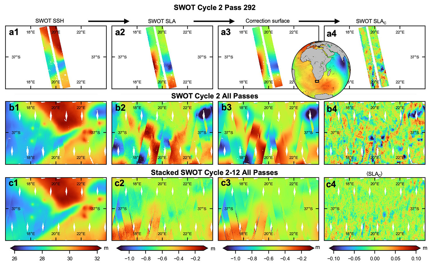
Figure 2 Long-wavelength correction of SWOT passes to fix the observations to the reference period. In figure (a) a single pass is shown, with the SWOT observations in (a1), the sea level anomaly (SLA) using DTU25_LWMSS in (a2), the long-wavelength parametric surface in (a3) and the corrected SLA in (a4) showing small scale features. In (b) all passes for cycle 2 is shown, showing the large oceanographic variability. In (c) 10 cycles are stacked (7 months of data), showing residual mesoscale features remaining if no correction is made. The resulting corrected 〈SLA_c〉 in (c4) using all cycles is what is used for the DTU25_2 kmMSS.

In order to fix the SWOT observations to the same reference period as the DTU25_LWMSS, as well as removing long-wavelength mesoscale oceanographic features, each cycle and pass is corrected. An example of the correction surface is seen in Fig. 2a3. The parameters β that is estimated is a bias and tilt in along-track and cross-track directions. This will also take into account any residual roll errors that might still be present in the data. This acts as a high-pass filter, removing the long wavelengths corresponding to the order of the fitted plane, and the short wavelength features emerges (Fig. 2a4).

In Fig. 2b1–b4 the same steps have been done for all passes for SWOT cycle 2 to illustrate the large variability of the SLA in the region off South Africa, and the subsequent small scale details revealed when fixing the long wavelengths to the reference surface. In Fig. 2c1–c4 a stack of 10 cycles is shown to illustrate the consequences of stacking along with this correction. In Fig. 2c2 mesoscale features are visible as this is a mean of approximately 7 months of data, and will have covered a specific oceanographic seasonality. By applying the correction to the data, the mesoscale features are removed and we are left with the short wavelengths (Fig. 2c4) which is gridded and used to construct the updated DTU25_2 kmMSS.

The correction surface is determined one for each swath in 50 km×50 km tiles, where the estimation matrix A is created

$$\begin{array}{}\text{(2)}& {\displaystyle }{\displaystyle }\mathbf{A}=\left[\begin{array}{cccccc}\mathrm{1}& c_{\mathrm{0}}& a_{\mathrm{0}}& c_{\mathrm{0}}^{\mathrm{2}}& \mathrm{\dots }& a_{\mathrm{0}}^o\\ \mathrm{⋮}& \mathrm{⋮}& \mathrm{⋮}& \mathrm{⋮}& \mathrm{⋮}& \mathrm{⋮}\\ \mathrm{1}& c_N& a_N& c_N^{\mathrm{2}}& \mathrm{\dots }& a_N^o\end{array}\right]\in {\mathbb{R}}^{\left(N_c{N}_a\right)\times (\mathrm{1}+o)},\end{array}$$

and where c_(⋅) and a_(⋅) corresponds to the cross-track and along-track distances respectively, o determines the order of the plane used for the correction and N_c and N_a is the number of points in the cross-track and along-track direction. An order o=0 or o=1 is used depending on the oceanographic variability of the region (more details in later section). For the given area we then remove the rows from the matrix that contains either invalid points sorted out from the outlier sorting or points not wanted for the correction, such as being too close to the coast. The parameter is then determined from least-squares fitting on the SLA

$$\begin{array}{}\text{(3)}& {\displaystyle }{\displaystyle }\text{SLA}=\text{SSH}-{\text{DTU25}}_{\text{LW}}\text{MSS},\end{array}$$

as seen in Fig. 2a2. The correction surface is then determined from

$$\begin{array}{}\text{(4)}& {\displaystyle }{\displaystyle }\mathit{\beta }=({\mathbf{A}}^{\top }\mathbf{A}{)}^{-\mathrm{1}}{\mathbf{A}}^{\top }\text{SLA}\end{array}$$

where the along-track overlap of 80 % with a Hann window in order to ensure a smooth solution. The subsequent corrected SLA is determined from:

$$\begin{array}{}\text{(5)}& {\displaystyle }{\displaystyle }{\text{SLA}}_c=\text{SLA}-\mathbf{A}\mathit{\beta }.\end{array}$$

These corrected SLA_c observations are then used in the further processing of SWOT. To further reduce the temporal signal and reduce the noise we take the temporal average for each observation-location over all cycles available (N);

$$\begin{array}{}\text{(6)}& {\displaystyle }{\displaystyle }\langle {\text{SLA}}_c\rangle ={\displaystyle \frac{\mathrm{1}}{N}}\sum _n^N{\text{SLA}}_c\left(n\right).\end{array}$$

The 〈SLA_c〉 is used in the further gridding and subsequent update of the reference MSS. The influence of the parametric correction was largest in the beginning of the SWOT science orbit, where a low number of cycles was available (<10 cycles). However, with the large number of cycles available at the time of writing (31 cycles) the importance of the correction has decreased significantly compared to at the beginning of the SWOT mission.

2.2.3 The DTU25_2 kmMSS

We use the L3 Expert (2 km) data product in the open ocean (>5 km from the coast), as the upwards continuation of the gravity signals will result in signals at shorter wavelengths to be too attenuated to be captured. The data is provided on a fixed grid at 2 km spacing and therefore is a significantly reduced dataset as well as computationally easy to compute the temporal average. This reduces the time and memory complexity of computing the MSS solution in the open ocean.

The gridding of the observations is done by least-squares collocation, similar to the construction of the older DTU models (Andersen et al., 2023). Essentially the updated MSS is constructed by determining the data covariance C₀ and defining the covariance function C(s). The covariance function used is

$$\begin{array}{}\text{(7)}& {\displaystyle }& {\displaystyle }{C}_r\left(s\right)=\left(\mathrm{1}+{\displaystyle \frac{s}{r}}\right)\exp \left(-{\displaystyle \frac{s}{r}}\right)\text{(8)}& {\displaystyle }& {\displaystyle }C\left(s\right)=C_{\mathrm{0}}\left[\mathit{\alpha }{C}_{r_{\mathrm{1}}}\left(s\right)+(\mathrm{1}-\mathit{\alpha })C_{r_{\mathrm{2}}}\left(s\right)\right]\end{array}$$

which consists of two second-order Gauss–Markov covariance functions C_|r(s) with their corresponding correlation lengths r₁ and r₂, each part weighted by the factor α, and the distance s is determined by the geodetic distance between points (ϕ₁,λ₁) and (ϕ₂,λ₂), and the correlation lengths is defined as $C\left(r\right)=\frac{\mathrm{1}}{\mathrm{2}}{C}_{\mathrm{0}}$. The two-part covariance function was determined by inspection of empirical covariances from SWOT 〈SLA_c〉, which on average matched two length scales λ₁=2.5 km and λ₂=10 km, resembling the SWOT data sampling spacing and the scale of the residual MSS submesoscale features. The weighing is determined as α=0.75. Additionally, an associated observation uncertainty ${\mathit{\sigma }}_{\mathit{ϵ}}^{\mathrm{2}}$ is determined and used to provide higher importance to observations with low noise. Uncertainty estimation of the SWOT data is further explored in Sect. 2.4.

The prediction grid $\widehat{\text{SLA}}$ is then determined from the 〈SLA_c〉 at locations $\mathit{x}=(\mathit{\varphi },\mathit{\lambda })$ at each gridpoint $\mathit{p}=({\mathit{\varphi }}_p,{\mathit{\lambda }}_p)$

$$\begin{array}{}\text{(9)}& {\displaystyle }{\displaystyle }\widehat{\text{SLA}}\left(\mathit{p}\right)=C(\mathit{x},\mathit{p}{)}^{\top }(C(\mathit{x},{\mathit{x}}^{\prime })+{\mathit{\sigma }}_{\mathit{ϵ}}^{\mathrm{2}}\mathbf{I}{)}^{-\mathrm{1}}\langle {\text{SLA}}_c\rangle ,\end{array}$$

where I is the identity matrix and the input to the covariance function is the pointwise geodetic distances $C(\cdot ,\cdot )=C\left(d_{\text{geo}}\right(\cdot ,\cdot \left)\right)$. To get the full model, we add back the long wavelength signals that were previously removed:

$$\begin{array}{}\text{(10)}& {\displaystyle }{\displaystyle }{\text{DTU25}}_{\text{2\hspace{0.17em}km}}\text{MSS}=\widehat{\text{SLA}}+{\text{DTU25}}_{\text{LW}}\text{MSS}.\end{array}$$

Additionally, the associated grid uncertainty ${\mathit{\sigma }}_{\widehat{\text{SLA}}}$ can be determined from

$$\begin{array}{}\text{(11)}& {\displaystyle }{\mathit{\sigma }}_{\widehat{\text{SLA}}}\left(\mathit{p}\right)=\text{diag}\left(C\right(\mathit{p},{\mathit{p}}^{\prime })-(C(\mathit{x},{\mathit{x}}^{\prime })+{\mathit{\sigma }}_{\mathit{ϵ}}^{\mathrm{2}}\mathbf{I}{)}^{-\mathrm{1}}C(\mathit{x},{\mathit{x}}^{\prime })).\end{array}$$

This framework involves repeated inversion of large matrices. However the mathematical equivalence to Gaussian Process Regression enables usage of software frameworks, such as GPyTorch which is utilized in this project to handle large datasets (Rasmussen and Williams, 2006; Gardner et al., 2021), necessary for utilizing SWOT data for global grids.

This is computed globally in tiles of 6° N×10° E size at 0.01° resolution (∼1.1 km at the equator), with a 50 % overlap between tiles. The overlapping tiles are then combined with a cosine weighting function to ensure no edge effects. Tiles with either no SWOT data (the entire tile is above/below ±77.6° N) or completely over land, we return the DTU25_LWMSS solution, but without the lowpass filter normally applied on the reference field.

In order to handle the increased amount of data when inverting the matrix in collocation, the gridding process is based on an iterative nearest-neighbor scheme. In each tile 10×10 grid points are selected, and a common nearest-neighbor search in the SWOT datapoints is done, starting with the 100 nearest points. A check is done to determine if at least 5 % of the points are further away than 50 km, to ensure no clipping of the covariance function. If not, we increase with 50 points and check again iteratively. The nearest neighbor search is done with the FAISS library, which significantly increases the lookup speed (Douze et al., 2024). A common number of points is the nearest 300 points.

The effect of the correction for MSS determination is shown in Fig. 3. This is the same area as in Fig. 2. The rows (a-d) show the MSS (determined from $\widehat{\text{SLA}}+{\text{DTU25}}_{\text{LW}}\text{MSS}$), associated uncertainty ${\mathit{\sigma }}_{\widehat{\text{SLA}}}^{\mathrm{2}}$, the $\widehat{\text{SLA}}$ and highpass filtered MSS at 20 km wavelength. The columns 1–4 are the different correction levels, with the first column only removing one overall bias from the SWOT data, and the next three columns using correction order o=0 to o=2. The region just off South Africa has high oceanographic variability, resulting in a high need for correction. Quiet regions show almost no need for correction. However, we see that a simple bias results in mesoscale signal still present in the data (resembling that of Fig. 2) as well as edge effects due to small differences in height in the different passes.

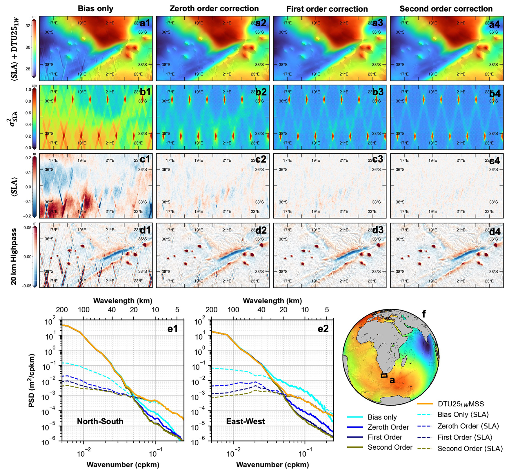
Figure 3 Effect on the MSS with varying levels of corrections on the SWOT data. Row (a) shows the MSS height, (b) shows the gridding uncertainty, (c) the gridded mean SLA and (d) the highpass filtered MSS. The four columns 1–4 are four levels of correction. Panels (e) show the associated power spectra density (PSD) plots of the MSS in the north-south and east-west direction as well as of the mean SLA.

The effect of higher order correction reduces uncertainty due to more oceanographic variability being removed, the mean SLA becomes smaller and the edge effect decreases. The effect on the spectral properties of the MSS is seen in Fig. 3e1 and e2, where the north-south and east-west direction power spectral density is computed. It can be seen that higher order corrections have smaller differences at long wavelengths. The effect at short wavelength is most pronounced in the east-west direction, due to the uncorrected edge effects being primarily in the east-west direction, and aliased to higher wavelengths in the north-south.

While higher order correction might seem better, higher orders correction might remove too much of the signal from SWOT. Comparing the area with Sentinel-3A&B data in Fig. 3, the second order correction showed a worse correspondence, compared to the first order. Globally in quiet regions, the first order was worse compared to the zeroth order, indicating too much of the signal was removed. In each tile when computing the DTU25_2 kmMSS, the initial correction is the zeroth order, but if the 90th-percentile of absolute SLA exceeds 10 cm, a first order correction is used instead.

Inspecting the power spectra in Fig. 3e1 and e2, the main difference between the reference surface and the corrected MSS is the lower power level at short wavelengths, cased by the lower noise in the SWOT data. The effect is predominantly located at wavelengths shorter than 𝒪(20 km). This corresponds to the band in which SWOT has shown to have excellent performance, and from where we can utilize the observations best (Nencioli et al., 2025). At the shortest wavelengths (𝒪(2 km), outside of scope of figure) there is a small increase in power due to small uncorrected height differences between gridded swaths at wavelengths matching the correlation length. This could be compensated by increasing the correlation length, however this will degrade the quality of the SWOT data for each swath. Due to the very small wavelength, this effect is ultimately removed when interpolating the MSS onto observations in practical use, and has thus not been corrected in this version, however will be a subject for further versions.

2.3 Stage 3: coastal zone

For the last stage we use the Unsmoothed 250 m SWOT data in the coastal zone (closer than 40 km from the coast). This is primarily due to the ability to map complex coastlines (Hart-Davis et al., 2024), with high spatial resolution. Due to the large datasize as well as inherent higher noise level due to the lower level of smoothing, several steps are taken to integrate this data with the previously created DTU25_2 kmMSS. As in stage 2, we now use the DTU25_2 kmMSS in a remove-restore fashion to produce the DTU25_250 mMSS.

Due to the 250 m data not being provided on a fixed geographical grid, stacking the data is not straight forward, as with the 2 km data. An additional step before gridding with collocation is performed. The tile size is smaller, in order to compensate for the larger file sizes, at 2° N×4° E, and the data is then binned with a 500 m bin size after outlier filtering and the mean and standard deviation in each bin is computed. Considering the correlation lenghts of 2.5 and 10 km, the initial coarse binning of the data initially will be compensated for.

As the 2 km SWOT data is less noisy in the open ocean than the 250 m data, due to spatial averaging, we want to rely on this data far away from the coast. This is done by an exponential distance weighting function of the form

$$\begin{array}{}\text{(12)}& {\displaystyle }{\displaystyle }{w}_{\text{L3a}}\left(d\right)={\displaystyle \frac{\mathrm{1}}{a}}{\mathrm{e}}^{-db},\end{array}$$

where a and b are determined such that we get a weighing of 1 at 10 km distance from the coast, and a weighing of 0.5 at 15 km distance from the coast (see Fig. 4c). The weighing for 2 km data is then determined as $w_{\text{2\hspace{0.17em}km}}\left(d\right)=\mathrm{1}-w_{\text{250\hspace{0.17em}m}}\left(d\right)$, and w_250 m(d) is truncated at 40 km distance, in order to reduce processing time, with the final DTU25MSS combined as:

$$\begin{array}{ll}{\displaystyle }& {\displaystyle }\text{DTU25MSS}=\\ \text{(13)}& {\displaystyle }& {\displaystyle \frac{w_{\text{2\hspace{0.17em}km}}{\text{DTU25}}_{\text{2\hspace{0.17em}km}}\text{MSS}+w_{\text{250\hspace{0.17em}m}}{\text{DTU25}}_{\text{250\hspace{0.17em}m}}\text{MSS}}{w_{\text{2\hspace{0.17em}km}}+w_{\text{250\hspace{0.17em}m}}}}.\end{array}$$

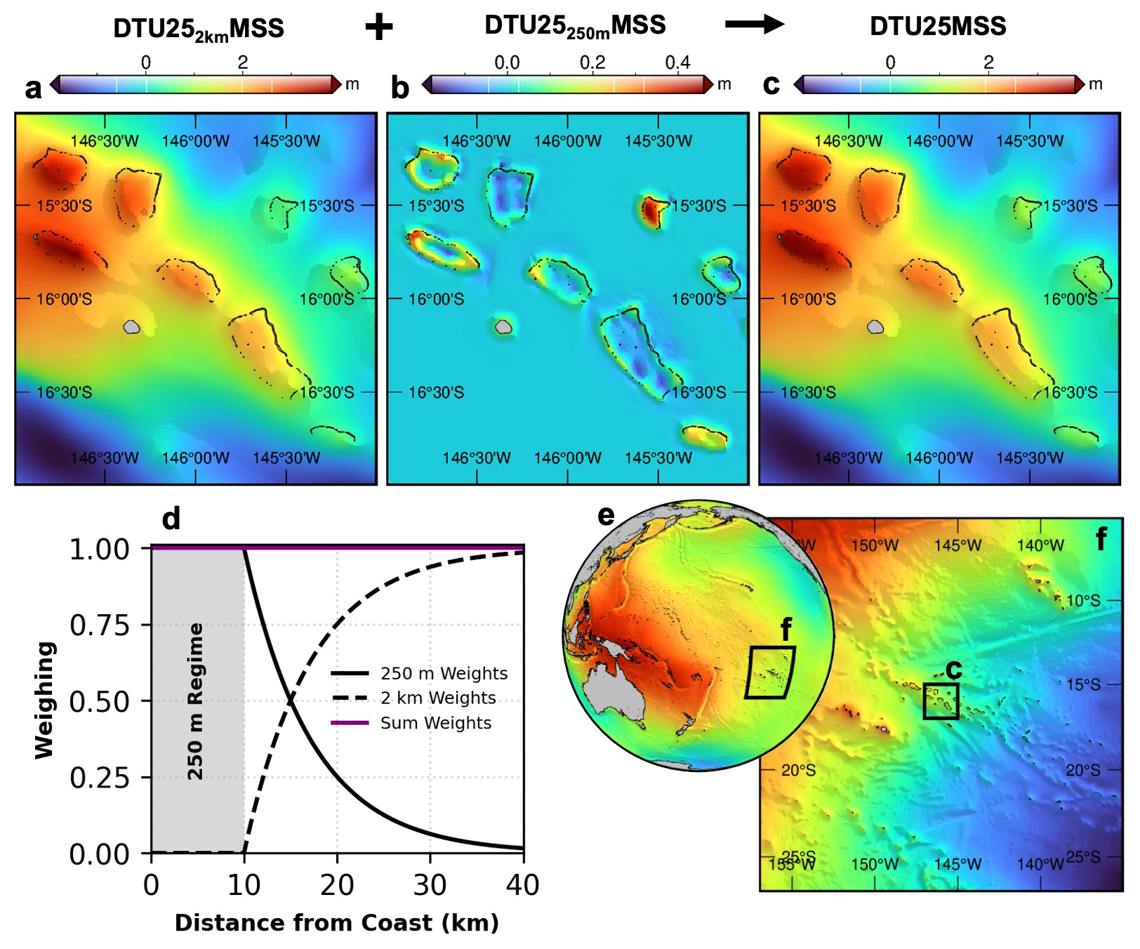
Figure 4 Example of the combination of the DTU25_2 kmMSS (a) and the new part in DTU25_250 mMSS (b) MSS models to create the DTU25MSS (c). Figure (d) shows the associated distance weighting for the 2 km and 250 m data products from SWOT. Figure (e) and (f) show the area depicted in this example.

This ensures we only fully rely on the 250 m data closer than 10 km from the coast. The combination of the DTU25_2 kmMSS and DTU25_250 mMSS to produce the DTU25MSS is seen in Fig. 4. A map showing globally where we use the 250 m data is seen in the Appendix as Fig. A1.

2.4 Uncertainty estimation of SWOT data

To provide an uncertainty measure for each observation, the individual uncertainty depends on a number of features such as the number of cycles in the stack, the local ocean variability and the location in the SWOT swath. These effects need to be combined to provide a point-source uncertainty to construct the covariance matrix and properly weight each observation when constructing the MSS grid.

The main causes of uncertainty were considered by empirical modeling in order to construct a globally consistent uncertainty model. The effects that are considered are as follows

• Oceanographic variability: When computing the temporal mean, we compute the stack uncertainty from the same data. This is defined as σ_n. By computing the temporal standard deviation, we can make sure we have high confidence in quiet oceanographic regions, while making sure we handle energetic regions reliably. Additionally, this is the standard deviation after performing the long-wavelength correction to the data, thereby resembling the variability left in the data.

• Cross-track swath uncertainty: As the uncertainty is a function of the cross-track location in the SWOT swath (Yu et al., 2024b; Peral et al., 2024), this is included as a function

  $$\begin{array}{}\text{(14)}& {\displaystyle }{\displaystyle }{\mathit{\sigma }}_c\left(c\right)={\mathrm{10}}^{-\mathrm{6}}\cdot \left(\right|c|-\mathrm{32}\mathrm{km}{)}^{\mathrm{4}},\end{array}$$

  where c is the cross-track distance from nadir in km. Here σ_c punishes points close to the edge of the swath, while being zero at the center of each swath. This is important in the case of overlapping swaths, as we have in each crossover point. In that case we will weight the observations in the center of one of the swaths, as opposed to the edge of the other. This also allows for a smooth fadeout in each of the data gaps between swaths, were we have to interpolate into the reference surface, due to having no new data.

• Distance to coast: Even though we can get close to the coast with swath altimetry, this is still a challenging region, due to coastal dynamics or poorly resolved land masks. Consequently for intermediate wavelengths, the data immediate next to the coast is weighted down by a inverse distance relation ${\mathit{\sigma }}_d\left(d\right)=d^{-\mathrm{1}}$. Here d is the distance to the coast in km.

• Inverse distance to coast: For the 250 m data, the goal is to utilize the high resolution close to the coast, but not degrade the high quality of the open ocean data. A second distance to coast feature is therefore introduced, increasing the uncertainty as a function of the distance to the coast ${\mathit{\sigma }}_{d\mathrm{2}}\left(d\right)={\mathrm{20}}^{-\mathrm{2}}{d}^{\mathrm{2}}$. As the gridding tends to zero in high uncertainty, this makes sure we rely more on the reference surface far from the coast.

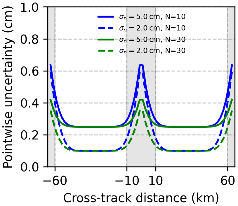
These features are determined for each SWOT observation, after the observations are stacked, with N observations in each stack. Due to the shifting orbit and the fixed geographical grid, the edges of the swath does not always contain observations, so N is not the same for the entire swath. This is considered when combining the observations to get the point-wise uncertainty

$$\begin{array}{}\text{(15)}& {\displaystyle }{\displaystyle }{\mathit{\sigma }}_{\mathit{ϵ}|d,c}^{\mathrm{2}}=\sqrt{({\mathit{\theta }}_{\mathrm{1}}{\mathit{\sigma }}_n{)}^{\mathrm{2}}+{\left({\mathit{\theta }}_{\mathrm{2}}{\displaystyle \frac{{\mathit{\sigma }}_c}{\sqrt{N}}}\right)}^{\mathrm{2}}+({\mathit{\theta }}_{\mathrm{3}}{\mathit{\sigma }}_d{)}^{\mathrm{2}}+({\mathit{\theta }}_{\mathrm{4}}{\mathit{\sigma }}_{d\mathrm{2}}{)}^{\mathrm{2}}},\end{array}$$

where θ_⋅ are parameters to determine the individual weight of the uncertainty parameters. This is to account for the fact that it is an empirically determined noise function, and the parameters are chosen such that the noise is as low as possible, while still providing a feasible solution (values: $\mathit{\theta }=[\mathrm{5},\mathrm{2},\mathrm{3},\mathrm{7.5}]$). An example with differing situations is seen in Fig. 5. In the case of the Unsmoothed 250 m SWOT data, the noise level is increased by a factor of 4 due to the smoothing factor of

$$\begin{array}{}\text{(16)}& {\displaystyle }{\displaystyle }{\mathit{\sigma }}_{\text{2\hspace{0.17em}km}}={\displaystyle \frac{{\mathit{\sigma }}_{\text{250\hspace{0.17em}m}}}{\sqrt{\frac{\mathrm{2}\mathrm{km}}{\mathrm{0.5}\mathrm{km}}\cdot \frac{\mathrm{2}\mathrm{km}}{\mathrm{0.5}\mathrm{km}}}}}={\displaystyle \frac{{\mathit{\sigma }}_{\text{250\hspace{0.17em}m}}}{\mathrm{4}}}.\end{array}$$

The uncertainty factor is due to the oversampling factor of 2 in the 250 m data, yielding an effective sampling resolution of 500 m (JPL, 2023). As the length scale is the same for both 250 m data and the 2 km data, the smoothing of SWOT is independent of datatype, however each 250 m data point gets less weight.

Figure 5 Combined uncertainty model for the SWOT swath with different examples of states.

We do not consider the temporal correlation, but this could be studied for future solutions. The mesoscale has the longest temporal correlation, but we correct the data in this regime, while the submesoscale is assumed to be decorrelated. This might not hold at high latitudes, due to the short temporal overlap between SWOT swaths. Further studies into uncertainty budgets and further validation of SWOT data will help improve the uncertainty models and enable better fitting to the data.

2.5 The gridded $\widehat{\text{SLA}}$ field

The $\widehat{\text{SLA}}$ field shows that the improvement from including SWOT is not globally or spatially homogeneous. Figure 6 illustrates that the majority of the differences are below 1 cm, with the major changes in the oceanographic meandering regions (such as the Gulf Stream and Kuroshio Current) as well as high latitude ice-covered regions.

In the histogram of the differences in Fig. 6c, the differences in the Pacific has smaller tails and more contained within 1 cm as compared with the region in the Gulf Stream. A large part has a difference of zero, due to SWOT being constrained to $\mathrm{77.6}\mathrm{°}\mathrm{N}/\mathrm{S}$ and therefore providing no additional information.

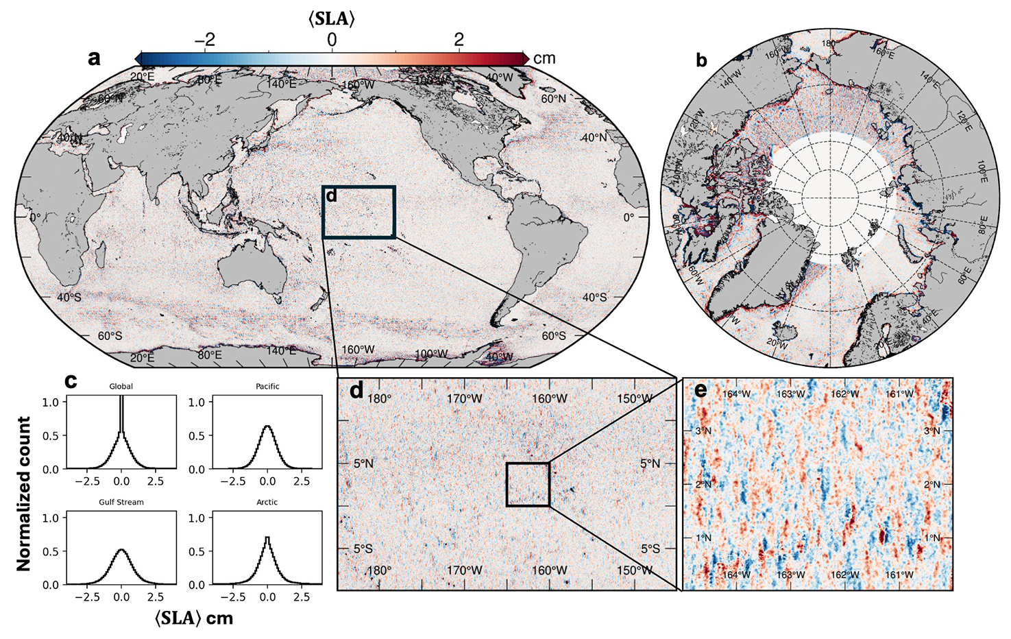
Figure 6 Differences between the DTU25MSS and the long-wavelength DTU25_LWMSS, showing the effect of including SWOT. In (a) a global map of the differences show that the majority of the differences are small (<1 cm), with the largest being in the areas with high ocean variability. In (b) the arctic region we see that we have no difference above 77.6° N, due to having no SWOT data. In (c) we show the distribution of the differences in different basins. In (d) and (e) a smaller area in the pacific shows the pattern of differences, a larger effect in the east-west direction compared with the north-south.

The differences in the open ocean (see Fig. 6d) looks more like noise, with some geodetic features apparent. However, the main cause would be due to noise contained in the DTU25_LWMSS that relies on nadir altimetry, that is reduced in DTU25MSS. Looking closer in Fig. 6e, the differences seem to have a latitudinal pattern. This is due to the reference field being constructed by nadir altimetry, which primarily samples north-south at the equator, while SWOT is capable of mapping the full field in one pass. The improvement to the MSS is therefore not isotropic, as the improvement is greater in the east-west direction than in the north-south, at the Equator.

3 DTU25 mean sea surface model

The global solution for the mean sea surface model is seen in Fig. 7. The DTU25MSS is a global model, and includes the polar regions outside 78° N and S, as these are carried over from the DTU21MSS model (Andersen et al., 2023).

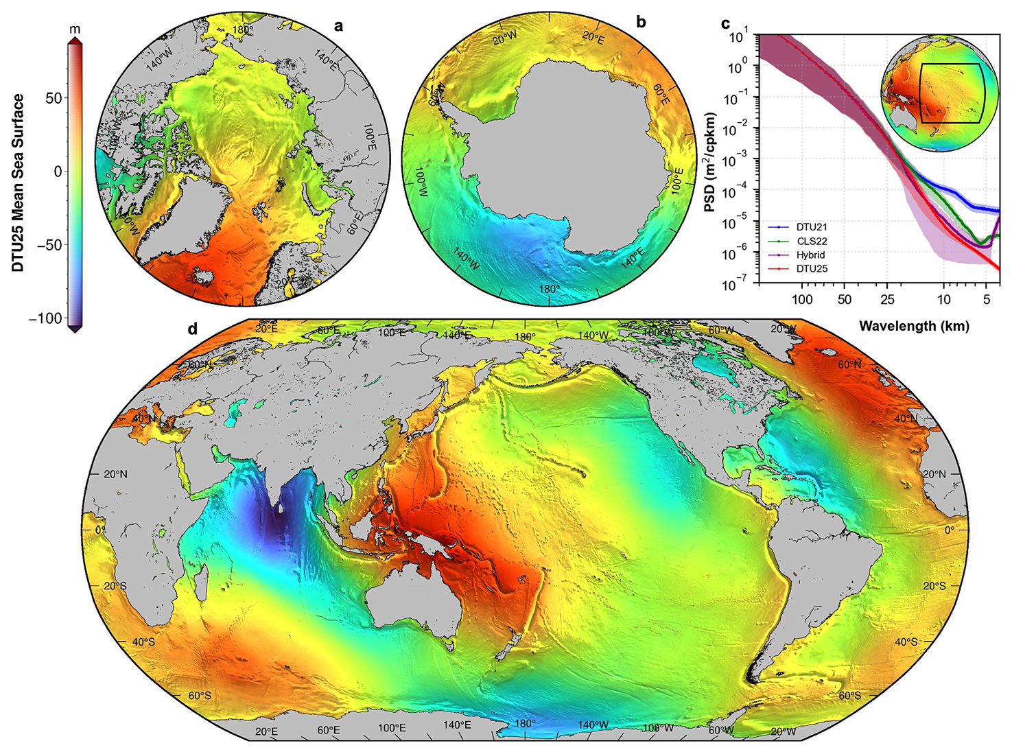
Figure 7 Global DTU25 Mean Sea Surface (a, b, and d). In (c) the PSD of DTU25MSS and the current state-of-the-art MSS models in the Pacific Ocean (black square) are shown. The PSD is calculated in 6°×6° tiles with Welch method. The shaded area shows the 1-σ difference between the tiles.

The PSD in Fig. 7 shows that the main changes from older models is in the wavelengths shorter than 20 km. The PSD is calculated using a modified Welch's method (Welch, 1967). The area indicated in Fig. 7c is divided into 6°×6° tiles, with a 50 % overlap in each direction, where the PSD is calculated in north-south direction in each tile with a Hann window matching the 6° size (with number of datapoints being: $\mathrm{6}\mathit{°}/\mathrm{0.01}\mathit{°}=\mathrm{600}$). This is zero-padded to 1024 to allow efficient computation. Any segments with a part that is closer than 5 km to the coast is discarded, as inland-areas are handled differently in each MSS model and would not be comparable.

After all tiles are computed, the mean PSD is computed, which is seen in Fig. 7c. The shaded region is the 1-σ of the PSD, illustrating the different power characteristics of the field at different locations, and therefore not necessarily the uncertainty. The most important differences are seen in the band from 10 to 20 km wavelength. This is the lower limit of what conventional altimetry (LRM and SAR mode) has been able to convincingly contribute to the models. The small wavelengths below 10 km primarily resembles the gridding or smoothing strategies utilized by the different methodologies. We see how DTU21MSS (blue) resembles the spectrum of nadir altimetry, where CLS22MSS is more smooth in this band. The Hybrid model, in the open ocean consisting mainly of the SIO MSS (Laloue et al., 2025), uses a spline-in-tension approach to grid the data, which could resemble the lower power level in this band (Sandwell, 2022), which quite closely matches that of the DTU25MSS. The increase in power at the shortest wavelengths could be a result of the stitching of different MSS in the HybridMSS, however this has not been further studied (Laloue et al., 2025). The low power level for the DTU25MSS at these short wavelengths are a result of the covariance function used for the gridding, making a smooth grid at wavelengths 10–5 km. We will later see (Sect. 4.2) that identical power spectra might not yield actual signal.

3.1 Model uncertainty

Along with the predicted field shown in the previous section, the associated uncertainty grid is provided and shown in Fig. 8. This resembles the results presented in Archer et al. (2025), and illustrates the submesoscale variability caused by internal waves and ocean currents along other effects. The submesoscale variability is still visible, as we have removed, or at least constrained, mesoscale activity by restricting long-wavelength signals from SWOT.

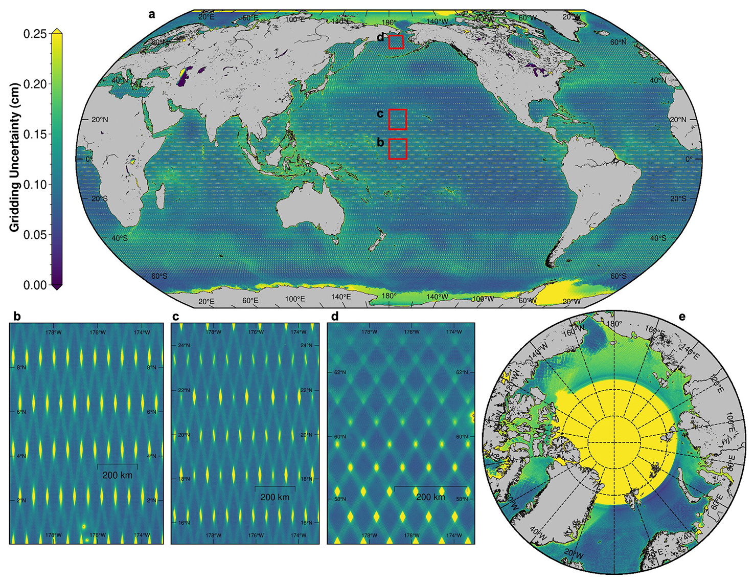
Figure 8 Gridding uncertainty (${\mathit{\sigma }}_{\widehat{\text{SLA}}}^{\mathrm{2}}$) for DTU25_2 kmMSS. The focus on areas (b–d) shows the diamond shaped data-gaps left due to the coverage of the SWOT mission, as well as the closing of the gaps at specific latitudes. The arctic is shown in (e), with the ice coverage clearly seen due to lower number of SWOT cycles available for the MSS determination. Uncertainty above 78° N is set to zero.

What is discernible in the model uncertainty estimate is the diamond shaped data gaps. This is most pronounced at the Equator (see Fig. 8b) where both the lack of overlap of SWOT as well as the overlapping nadir gaps cause two different coverage gaps or diamonds. One of them closes fairly quickly at 20° N (Fig. 8c), but they are still present up till around 60° N, at reduced size, whereas there is a full coverage at high latitudes. In areas with no SWOT data, such as these gaps, the MSS converges to the reference MSS, which in this case is the DTU25_LWMSS.

In the Arctic Ocean there is a larger area with a higher uncertainty than in the global oceans, which resembles the ice coverage in the region. This stems from the ice cover in winter, reducing the number of cycles that could be used to map this area thereby only relying on summer data (essentially reducing the number of cycles by half). A small area between 20–40° W is completely unmapped, likely due to multi-year ice coverage, just as in the Weddell sea.

3.2 Moving the reference to 2023

Global sea level rise has resulted in a global mean sea level difference of 𝒪(5.8 cm) since 2003, consistently moving current sea level observations away from the agreed mean level (Nerem et al., 2018; Veng and Andersen, 2021). Additionally, sea level rise and sea level acceleration varies globally, resulting in a MSS reference that degrades over time. DTU25MSS has been derived using a consistent estimation of the mean, linear sea level change and the annual signal (see Eq. 1). We used the estimated sea level change to move the reference forward from 2003 to 2023 creating an experimental MSS which is tailored to the SWOT period and which matches current sea level more closely. Outside the 66 parallels we used the timeseries from ERS2, ENVISAT and Cryosat-2 from the Radar Altimetry Database archive (RADS) (Scharroo et al., 2012), to estimate linear sea level in a similar way to what was done along the reference groundtracks (fitting the t₀ to 2003). This way we were able to shift the reference period globally with the various datasets. The resulting MSS is called DTU25MSS_2023X and the difference with DTU25MSS is illustrated in Fig. 9. The shift of the reference has a mean of 5.6 cm with a maximum of 20 cm north of Alaska in the Beaufort Gyre and a minimum in the Southern Pacific Ocean of −4 cm.

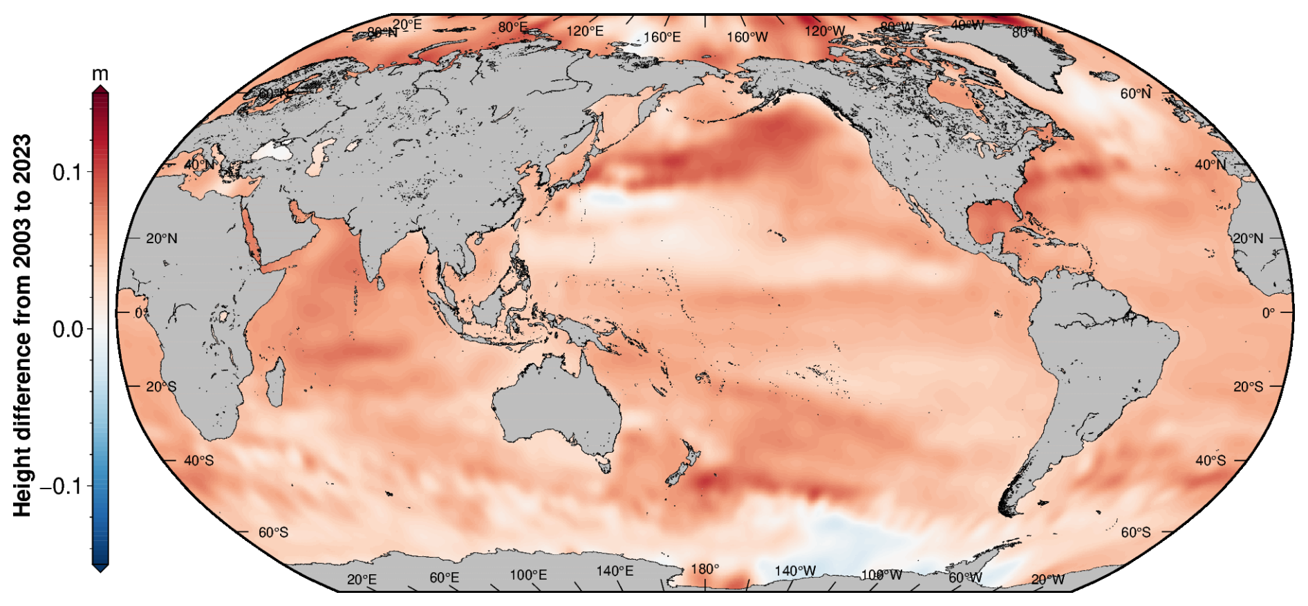
Figure 9 The difference between the experimental DTU25MSS_2023X and DTU25MSS. DTU25MSS_2023X has the “center period” brought forward to 2023 using linear sea level change. Hence the difference illustrates linear sea level change between 2003–2023.

3.3 Small scale coastal zone MSS

The benefits of utilizing the high resolution data from SWOT are not necessarily discernible from the full heights. In order to visually inspect the difference of introducing SWOT to the short-wavelength signal, we instead high-pass filter the MSS. We use a gaussian filter with a Full Width at Half Maximum of 20 km, which corresponds to a $\mathit{\sigma }\approx \mathrm{20}\mathrm{km}/\mathrm{2.36}=\mathrm{8.47}\mathrm{km}$, to isolate the regime where the difference from SWOT is most noticeable.

3.3.1 Atolls

Atolls are ring-shaped island that encircle a central lagoon of open water and is a good way to visually demonstrate the benefit of SWOT for small scale signals. French Polynesia is located in the Pacific Ocean and should be well resolved by nadir altimetry as well as by the new 2 km SWOT ocean data. This is true, up to a certain extent, as the enclosed waters of the atolls are either poorly resolved or not captured at all with the coarse resolution used in the open ocean.

In Fig. 10 we see the MSS variation for the island chains in French Polynesia with either DTU21MSS (a) or DTU25MSS (b), highpass filtered to showcase the spectral band where we gain new information from SWOT. In the open ocean we generally see a lower noise level in DTU25MSS compared to DTU21MSS, and some small scale seamounts are discernible. However looking specifically at the atolls, we see how the 250 m data enables us to obtain a much sharper delineation between open ocean and the lagoons (Fig. 10a1, b1, and d), matching the enclosed areas as observed with Sentinel-2 (Fig. 10c).

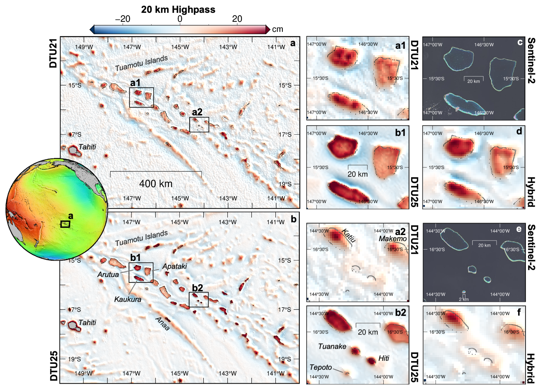
Figure 10 Comparison of DTU21MSS (a), HybridMSS and DTU25MSS (b) in French Polynesia. Zoom in shows small scale details captured by SWOT not previously possible by nadir altimetry, with optical images from Sentinel-2 showing the central lagoons of the Atolls.

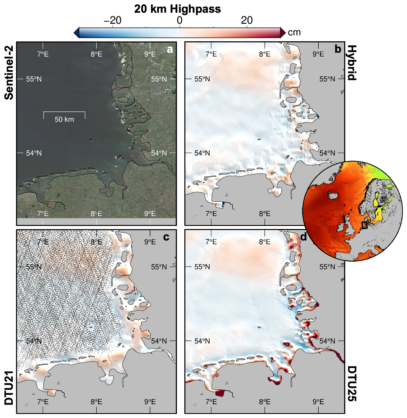
Figure 11 The Wadden Sea seen from Sentinel-2 (a) and highpass filtered at 20 km with the HybridMSS (b), DTU21MSS (c), and DTU25MSS (d). Black points in (c) shows where nadir altimetry observations are located that is used in the creation of the DTU21MSS.

While the atolls in region a1/b1 was captured by nadir altimetry due to their size (wider than 20 km), in region a2/b2 we see small scale atolls that were not captured at all in the older MSS. With the 250 m data, we capture the circular shape of the small atolls, down to the small Tepoto atoll with a lagoon width at 1 km. The higher mean water level compared with the open ocean in the surrounding area is in line with the known behavior of atolls (Callaghan et al., 2006), and the introduction of the smaller scale atolls should improve the MSS reference for regional studies in the global oceans.

3.3.2 Tidal flats

Tidal flats are complex coastal features that are both small scale and dynamic in time. They encompass river outlets as well as non-permanent islands, and have been challenging to map from satellite altimetry. With swath altimetry from SWOT, it has been show that it's possible to map the tidal flats, as well as constructing an elevation model from the data (Salameh et al., 2024; Shi et al., 2025).

Looking at the Wadden Sea, a coastal region in the Netherlands, Germany and Denmark as observed from Sentinel-2 in Fig. 11a, the complex coastal structure is seen. Shown in Fig. 11c, is DTU21MSS with black dots illustrating all available altimetry data used to construct the model. What is clear is the absence of valid data in the coastal zone, which constrains older models in their validity in this region. With SWOT we are able to observe all the way to the coasts which encompasses several smaller islands and peninsulas.

However these features are dynamic in time, at different timescales. While they might be physical present during the sampling time of SWOT, this might not be valid during the entire 30 years where satellite altimetry has been available. This might lead to a problematic reference surface, however as we saw before the conventional altimetry already exhibits problems in this area. Further discussion and studies into incorporating new complex features into a reference surface would be needed, as well as their impact on the resulting observations, depending on the use of the product. We have elected to keep it as a real physical signal in the product, to use as a reference for the SWOT mission.

3.3.3 Fjords and archipelago's

Another challenging region which historically has caused problems are fjords, due to their long and shallow reaches (Tomić and Andersen, 2023), as well as archipelagos as the many small islands causing contamination in the return waveforms in the conventional altimetry (Tomić et al., 2024).

Encompassing both, the west coast of Norway has a lot of islands as well as very shallow and long fjords. This has caused earlier MSS solutions to rely on either extrapolation or data filling from alternative data sources, due to having no reliable satellite altimetry data in the coastal region, as seen in Fig. 12b, with the point illustrating all available altimetry used for DTU21MSS between 59.7–62.3° N for reference.

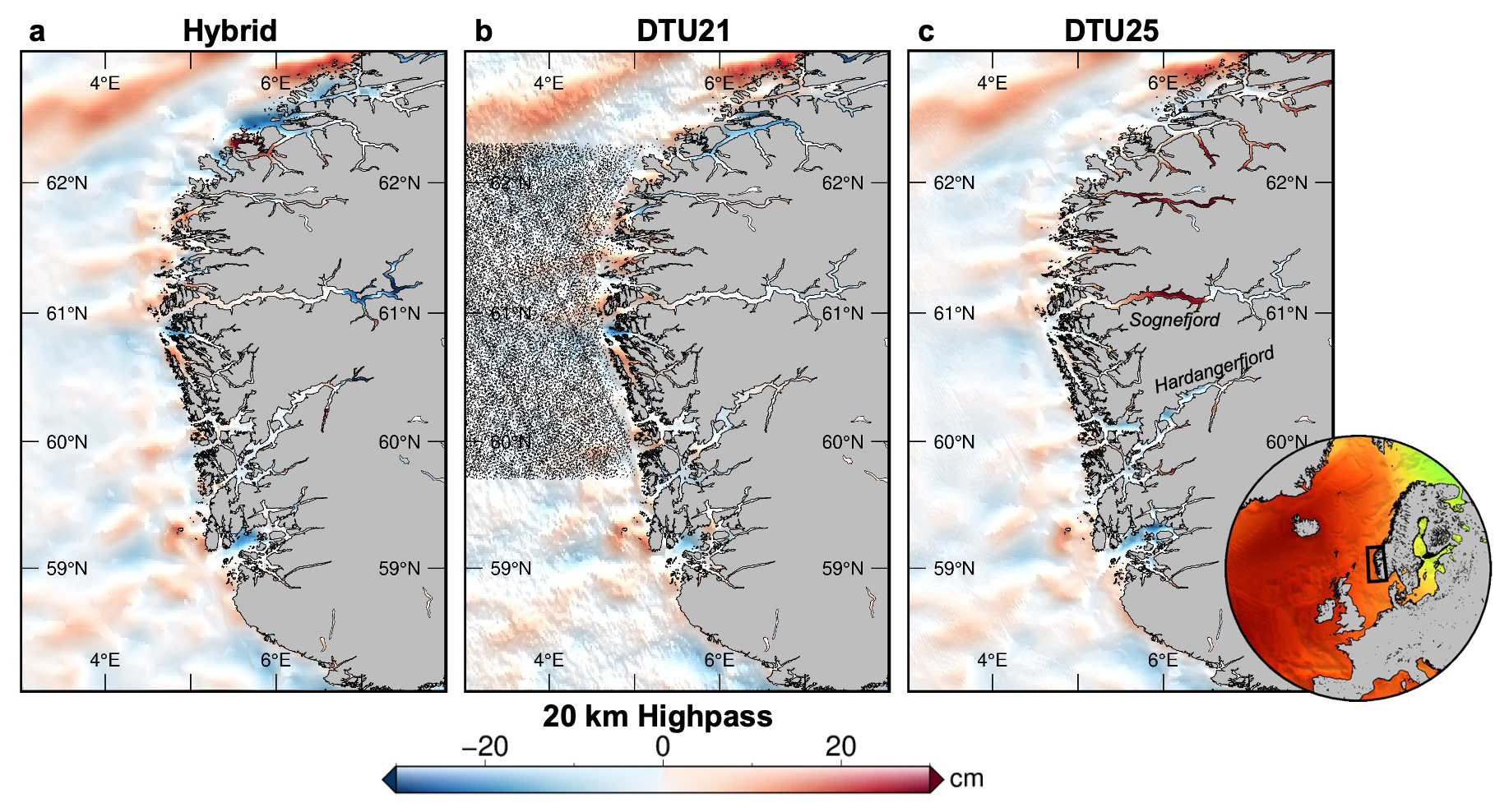
Figure 12 The western coast of Norway highpass filtered at 20 km with the HybridMSS, DTU21MSS and DTU25MSS in (a), (b), and (c) respectively. Black points in (b) indicate where nadir altimetry observations are located (between 59.7–62.3° N) in the creation of the DTU21MSS.

We see that the MSS has been updated in the fjords, with Hardangerfjord becoming lower and Sognefjord increasing in height, indicating new height data in these fjords. Validation of these regions is challenging, as no other radar altimeter can get reliable data in the shallow fjords, however future studies of the ability of SWOT to map the fjords might be possible with the small footprint of ICESat-2 (Tomić and Andersen, 2023).

What we see at Sognefjord is a sudden stop in the update, which is caused by the lack of new data east from here, most likely caused by the distinction between open-ocean and inland-water classification. As new versions of the SWOT data processing is released, improving its quality, future versions of the MSS would be improved in turn.

4 Validation

While the sections before primarily was a qualitative inspection of the new MSS, in order to determine the quantitative difference between the models, we compare with external observations. These include conventional nadir altimeters that have not been included in the reference MSS (Sentinel-3A&B), as well as the Cal/Val orbit of SWOT, which includes three months of daily repeat orbits in 28 tracks globally. Utilizing this, we have very high precision observations from which we can determine statics of the global MSS solution.

4.1 Comparison with Sentinel-3A&B

The improvement of the MSS will benefit the high resolution observations made by SWOT, but will in turn also improve reprocessed data on other altimeter platforms as well. Signals falsely attributed to oceanographic features or noise, might be resolved in the new MSS and will decrease the signal power of the observations.

In order to determine the effect of this, we compare with stacks of Sentinel-3A&B data. We use the full stack to reduce the altimetric noise and dynamic oceanographic features as much as possible, to determine the amount of agreement between the observations of the static signal in Sentinel-3A&B and the different MSS models. The Sentinel-3A&B data utilizes the full corrections from the Radar Altimeter Database System (RADS), but referenced against the ellipsoid in order to use our different MSS models for testing (Scharroo et al., 2012).

As the MSS model is defined in a certain reference period that might not be matching that of either Sentinel-3A or 3B, we expect to see a bias corresponding to sea level rise, as well as a long-wavelength signal that corresponds to the shift of the large scale oceanographic features.

To see the effect of utilizing SWOT, which is generally smaller than the difference in mesoscale contents in Sentinel-3A&B and the MSS models (See Fig. 13a), we also high-pass filter the Sentinel-3A&B passes before computing the statistics. The high-pass filter used is a Savitzky–Golay filter, which is a moving window polynomial fit, which better preserves amplitudes of the signal (Savitzky and Golay, 1964). We use a second order filter with a window length of 50 km to better match the spatial scale where we have utilized SWOT data (see Fig. 3). This is computed globally along with the uncorrected heights for each individual pass and the statistics are seen in Table 2. An example of the effect of this correction on a single pass is seen in Fig. 13b.

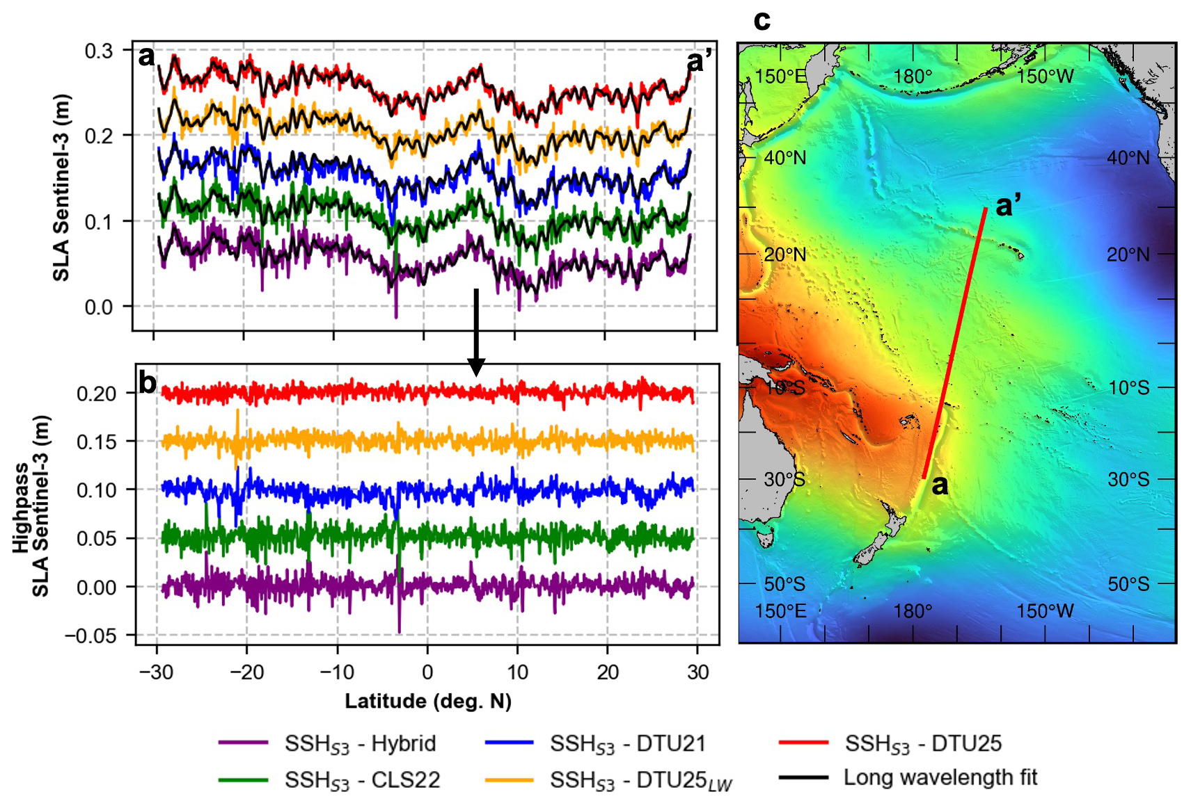
Figure 13 Sentinel-3A&B SLA example profiles computed with different MSS references, each profile offset with 0.05 m to help visual inspection. Black line indicates the long-wavelength fit subtracted from the SLA to compute (b), the short-wavelength difference. Example profile locations shown in (c).

Table 2 Standard deviations computed from the mean Sentinel-3A&B profiles subtracted with different MSS reference models. Bold indicates best performing in each column.

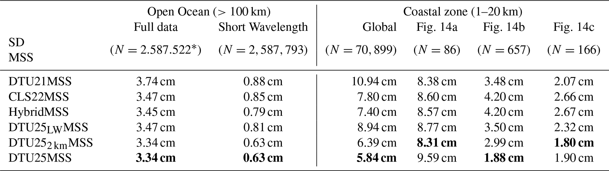
^* 1202 outliers removed from all where mean absolute difference was larger than 1 m.

4.1.1 Coastal zone

In order to determine the effect of using SWOT in the coastal zone, we subdivide the Sentinel-3A&B observations mentioned before, to encompass the area around the coastal zone (1–20 km). Here only the full heights are used, as it is not possible to high-pass filter such short profiles. The resulting comparison globally as well as in the three cases shown in Sect. 3.3 are seen in Table 2. Here both the DTU25_2 kmMSS and the DTU25MSS are used, in order to see the effect of including the coastal features with the 250 m data. In Table 2 the HybridMSS and CLS22MSS are almost identical, due to the HybridMSS primarily consisting of the CLS22MSS in the coastal zone (Laloue et al., 2025).

As Sentinel-3A&B operates in SAR mode, the footprint along the track is only 𝒪(300 m), but the footprint size in the along-track direction is 𝒪(7 km). By including features of size 𝒪(2.5 km) in the MSS, even though the feature might be physical, it might not necessarily reflect the observation as seen from Sentinel-3A&B.

In order to see the effect of this, the standard deviation (SD) of the Sentinel-3A&B observations with reference to the MSS models, as a function of distance to the coast, is seen in Fig. 14. This is three very different areas, and we see the benefit as well as the problems in some of the cases.

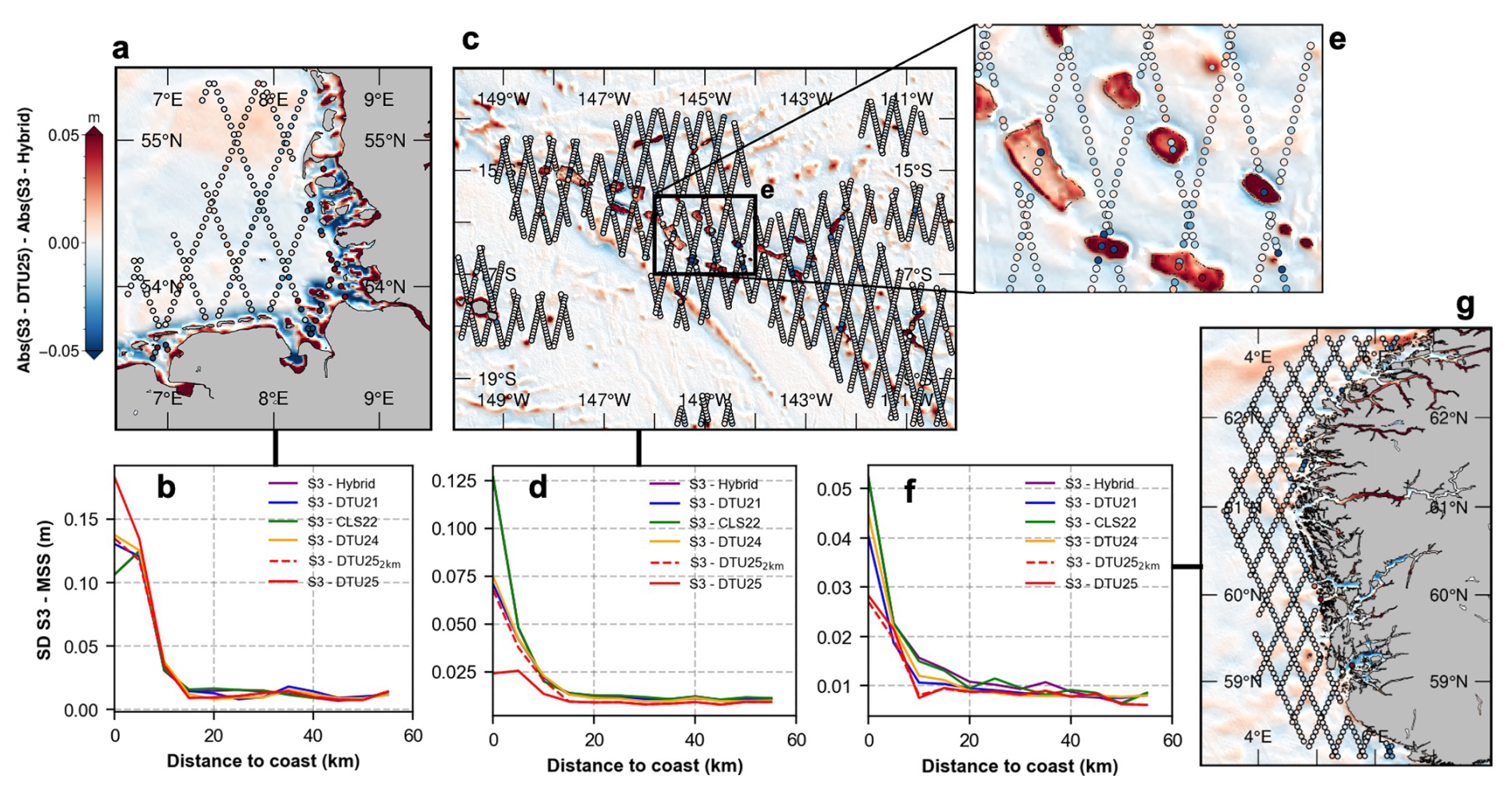
Figure 14 Standard deviation of the Sentinel-3A&B mean profiles subtracted from different MSS models, as a function of distance to the coast. Map (a) corresponds to the plot in (b) where the points are the bias-corrected absolute difference of Sentinel-3A&B and DTU25MSS subtracted from the bias-corrected absolute difference of Sentinel-3A&B and HybridMSS. Where blue indicates a better fit for DTU25MSS and red indicates a worse fit. This is equivalent for (c–e) and (f–g). Matching maps and plots are indicated by the connecting line.

In Fig. 14a the Weddel sea from Fig. 11 is seen, with overlay of Sentinel-3A&B measurement locations. The color of each locations is the difference between the agreement between Sentinel-3A&B mean profiles and the MSS models DTU25MSS and HybridMSS, determined as

$$\begin{array}{}\text{(17)}& {\displaystyle }{\displaystyle }\text{diff}=|{\text{SSH}}_{S\mathrm{3}}-\text{DTU25}{|}_{\mathit{\mu }=\mathrm{0}}-|{\text{SSH}}_{S\mathrm{3}}-\text{Hybrid}{|}_{\mathit{\mu }=\mathrm{0}},\end{array}$$

where SSH_S3 is the mean profile of Sentinel-3A&B and μ=0 means we subtract the mean before computing the absolute differences. This results in white being equal agreement between Sentinel-3A&B and the MSS models, red is worse agreement for DTU25MSS compared with the HybridMSS, and blue is better agreement for DTU25MSS. This is computed for Fig. 14b and c as well.

In Fig. 14 there are corresponding plots showing the standard deviation of the areas a-c, as a function of distance to the coast. We see how all models generally have the same uncertainty far from the coast, as we also saw in Table 2 that the overall difference between the models are small. However close to the coast (<10 km) the differences increase, which also matches where we start seeing colors in the points on the map.

For the Weddel Sea in Fig. 14a, almost all models have the same performance, except the DTU25MSS which includes the 250 m data which we saw became much more complex in the tidal flats. Inspecting the location of the differences we see that some locations have a much better agreement while some are much worse, which is underlined if we computed the median absolute error instead of the standard deviation. However the cause of this could be due to the time-varying aspect of tidal flats or the large and anisotropic footprint and reflection of Sentinel-3A&B. Further studies into incorporating these complex regions into MSS reference surfaces might provide better agreement with nadir altimeters.

For atolls in the open ocean, the case is the opposite, with a large increase for the current models close to the coast, and a very small standard deviation when including the 250 m data. Looking closer to some examples in Fig. 14b1, the few points that lie in the central lagoons seem to have benefited overall quite well from the increased height.

4.2 Comparison with independent SWOT data

We withheld the fast sampled Cal/Val orbit from the global solution in order to get a better understanding of the performance increase obtained from including SWOT in the MSS solution. As there has never been a satellite altimeter with a higher resolution than SWOT this would be a good opportunity. Additionally, even though the MSS would be locally improved along the 28 tracks from the Cal/Val orbit and some of the data gaps would be filled, we turned to a more temporally and spatially consistent model globally, by utilizing only the science orbits.

As the Cal/Val orbit has the same inclination as the Science Orbit (at 77.6°) but with a small shift of the ascending node, we are able to get similar but not identical observations compared to the Science Orbit. Using this we can compare the spectral components and compute the cross-power spectra to determine the spatial resolution to which the DTU25MSS agrees with the Cal/Val orbit, without relying on any one single track from the science orbit.

In Fig. 15, two parallel passes, one in the Cal/Val (green) and one in the Science orbit (yellow) are shown. While the pass from the Science orbit is included in the creation of the DTU25MSS, the Cal/Val orbit is not. For both the included and independent data we see the PSD of the stacked SWOT SSH (S_SWOT) and the MSS sampled in the SWOT grid (S_MSS) in Fig. 15c and e, as well as the Coherence (d and f), determined from the PSD and cross-PSD

$$\begin{array}{}\text{(18)}& {\displaystyle }{\displaystyle }{C}_{\text{SWOT,MSS}}\left(k\right)={\displaystyle \frac{\left|S_{\text{SWOT,MSS}}\right(k){|}^{\mathrm{2}}}{S_{\text{SWOT}}\left(k\right)S_{\text{MSS}}\left(k\right)}}.\end{array}$$

For the PSD one can visually see how the spectra of the different MSS models compare with the power level of the SWOT stacks. The plot here resembles the one from Fig. 7c where we saw that it is not possible to distinguish between appropriate filtering and thereby matching the power level of SWOT, or actually containing signal within this power signal.

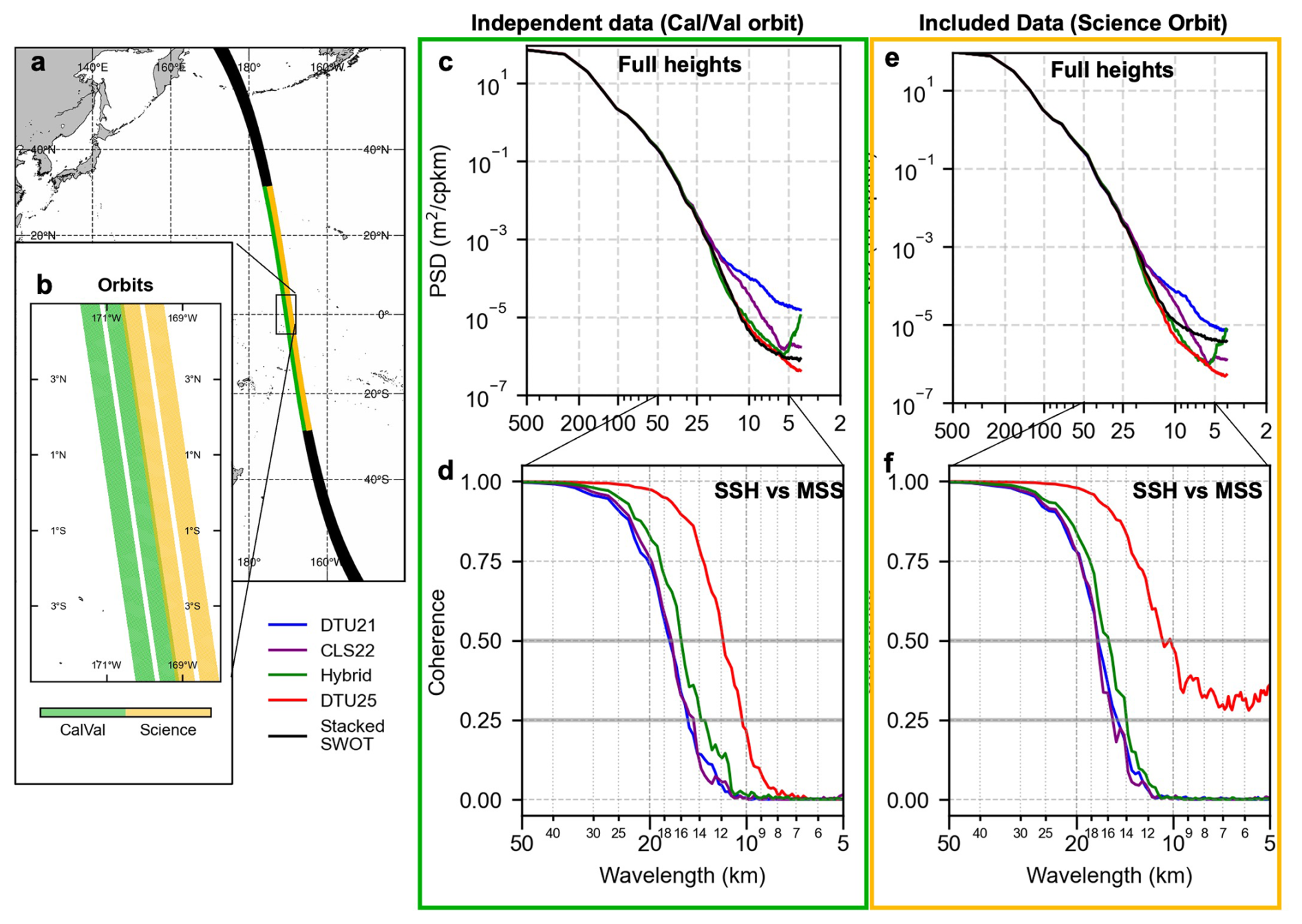
Figure 15 Power spectra and coherence determined from independent SWOT data (green) and included SWOT data (orange), with parallel groundtracks almost identical location (a, b). Plot (c) shows the power spectra of four MSS models interpolated onto the SWOT fixed geographical grid, along with the power spectra of the stacked (90 cycles) SSH observations from SWOT (black) in the Cal/Val orbit, not included in the MSS models. Plot (d) shows the corresponding coherence of the interpolated MSS models with SWOT. For (e) and (f) the same as before, but with the included SWOT data from the Science Orbit. Decoherence thresholds of 0.5 and 0.25 are marked in bold grey.

By inspecting the coherence we can determine the wavelength $\mathit{\lambda }=k^{-\mathrm{1}}$ of decoherence, here defined as 0.5. It can be seen that the MSS models relying on purely nadir altimetry, while exhibiting different power spectra, show almost the same spatial resolution when compared with SWOT. Here SWOT indicates an approximate 30 % improvement of spatial resolution for DTU25MSS, compared with all older MSS models (from 18 to 12 km).

For the SWOT data from the science orbit, we see that we cross the 0.5 coherence, indicating that we not purely rely on this pass. But also use data from the crossing passes. But we never reach 0 coherence, thereby still containing some of the data present in the SWOT data, even at short wavelengths.

This same methodology can be applied globally, as we have 28 independent Cal/Val orbits. This same spatial resolution is computed in 6° intervals along-track, with 50 % overlap, and can be seen in Fig. 16. We can then see that the spatial resolution obtained from this method is very geographically dependent, as we obtain a worse resolution in regions with high oceanographic variability, such as the Kuroshio Current in the Pacific Ocean, resembling the earlier assessment based on the same methodology (Nilsson et al., 2025). But in Fig. 16 we can see a clear relationship between the obtained spatial resolution and mean ocean depth at the sample location, showing that we are not necessarily determining the resolution of SWOT but the spatial size of the features in the MSS, which are smoothed due to upwards continuation from the ocean floor. However, looking at the points marked with a black border, we see the matching pairs and we see a consistent better spatial resolution for DTU25MSS compared with the current state-of-the-art Hybrid MSS.

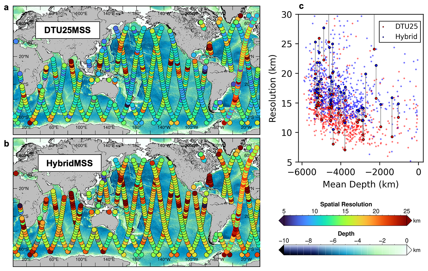
Figure 16 Spatial resolution determined as the wavelength at 0.5 coherence between SWOT Cal/Val orbit and the DTU25MSS or the HybridMSS in 6° latitude bands, with 50 % overlap. In (c) all resolutions for both MSS is shown as a function of mean ocean depth in the latitude band. Points with black border (in c) is points associated with the indicated track in (a) and (b) with red borders, and the connected vertical line indicates that the points are at the same location.

4.2.1 Effect on SWOT observations

To determine to effect of switching to a new MSS reference when using SWOT, we compare oceanographic features-of-interest based on different reference surfaces, including the experimental reference frame at the 2023 epoch. The three features are the zeroth, first and second order derivatives of the sea surface, reflected as the SLA, sea surface currents (SSC) and the relative vorticity (ξ). These are determined in two cases; (a) for a single pass thereby reflecting the effect on an instantaneous observation, and (b) for the full stack of observations. The stacking of SWOT data resembles an MSS which, compared with the MSS reference models, gives an indication of the residual effect of unmodeled geodetic features leaking into the ocean features as observed from SWOT.

Firstly for the single pass, the SLA is determined as

$$\begin{array}{}\text{(19)}& {\displaystyle }{\displaystyle }\text{SLA}=\text{SSH}-{\text{MSS}}_{(\cdot )},\end{array}$$

with the different MSS models as reference. The SSC are then determined from the derivative of the Absolute Dynamic Topograhy (ADT) in x- and y-directions to use the geostrophic equations:

$$\begin{array}{}\text{(20)}& {\displaystyle }{\displaystyle }u=-{\displaystyle \frac{g}{f}}{\displaystyle \frac{\partial \text{ADT}}{\partial y}},v={\displaystyle \frac{g}{f}}{\displaystyle \frac{\partial \text{ADT}}{\partial x}},\text{SSC}=\sqrt{u^{\mathrm{2}}+v^{\mathrm{2}}}\end{array}$$

where f=2Ωsin ϕ, g is the gravitational acceleration, x and y resembles the two axis of the SWOT sampling grid, and

$$\begin{array}{}\text{(21)}& {\displaystyle }{\displaystyle }\text{ADT}=\text{SSH}-\mathrm{N}=\text{SSH}-({\text{MSS}}_{(\cdot )}-\text{MDT}),\end{array}$$

where N is the geoid and MDT is the Mean Dynamic Topography (Mulet et al., 2021). The derivative is computed in the SWOT native grid of 2 km×2 km, however to reduce the smallest scale effects the SLA (before computing the derivative) is smoothed with a 6 km×6 km lowpass boxcar filter. Computing the derivative minimizes the effect of the long wavelength MDT, and the same MDT is used for all situations, but is still included in order to reflect the numeric value of the features. The assumptions needed for geostrophic balance does not hold at these scales, however this can be used as a proxy to determine the energy level of submesoscale features or resulting omitted geodetic signals present in the data, and how they would show up as sea surface currents when using the geostrophic equations at this scale.

Lastly the vorticity is determined as

$$\begin{array}{}\text{(22)}& {\displaystyle }{\displaystyle }\mathit{\xi }={\displaystyle \frac{\partial v}{\partial x}}-{\displaystyle \frac{\partial u}{\partial y}}.\end{array}$$

This is again determined from the native 2 km grid of SWOT, with the 6 km×6 km lowpass boxcar filter applied on the SLA. The derivative has been applied a second time, which results in a smaller overall swath. The small spatial scale of the derivative results in noisy estimates of the vorticity, but can be used to evaluate the relative difference between the MSS fields at these small scales.

The same is computed for the stack, however in the equations shown before the SSH is replaced by $\frac{\mathrm{1}}{N}{\sum }_i^N{\text{SSH}}_i$ for N passes in the stack. As this is the definition of the MSS (when N→∞), this indicates the effect of unmodeled geodetic features leaking into the oceanographic variables.

In Fig. 17a and d we see the effect of changing the MSS on SWOT data for a single pass (left) and for the full stack (right). On the left we see that there is not a large difference between the different MSS models, indicating that the signal observed by a SWOT pass is dominant, compared to the MSS errors. On the right the difference with DTU25MSS is much smoother, compared with the other reference surfaces. As we only updated the MSS with the short wavelengths, a long-wavelength mean signal is expected to be present in the data, which is what we see. This is clear when using the DTU25MSS_2023X, as the main difference between SWOT and the current MSS models is the larger scale changes, some of which can be attributed to sea level rise. In the following derivatives it can be seen how the DTU25MSS_2023X is only different from the DTU25MSS at long wavelengths.

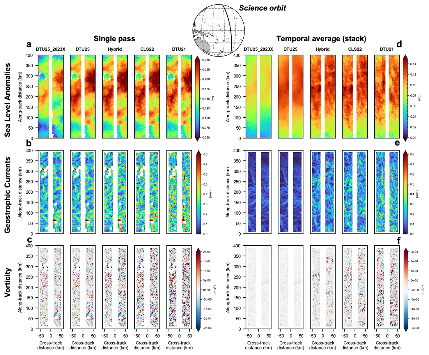
Figure 17 Three oceanographic variables (sea level anomaly a, d, geostrophic currents b, e and vorticity c, f) computed for a single SWOT pass from the science orbit (left, cycle 2 pass 28) and from the temporal average of 31 cycles (right) with different MSS models as reference.

For the SSC in Fig. 17b we see a slight decrease in the noise but the majority of the signal is still left in the data, however for the stack in figure Fig. 17e the strength of the residual signal is significantly decreased. This is even more discernible with the vorticity, as the signal for a single pass looks almost identical with only a small decrease, however there is a clear effect for the full stack.

As the majority of the improvement is at very short wavelengths by SWOT, and the derivative acts as a high-pass filter, it is expected that the improvement will become more clear at higher derivatives. The second order derivative resembles the process with which gravity is determined from sea surface observations, which illustrates why SWOT has been able to capture marine gravity at an unprecedented level (Yu et al., 2024a).

Repeating the same analysis, this is done for the independent SWOT data from the Cal/Val orbit in Fig. 18. We see the same as in Fig. 17, indicating this effect is not only caused by including the same SWOT data into the reference. However we also see the effect of hybridization of the HybridMSS, which causes small scale effects at certain locations (Laloue et al., 2025), primarily noticeable when stacking the highly accurate SWOT data.

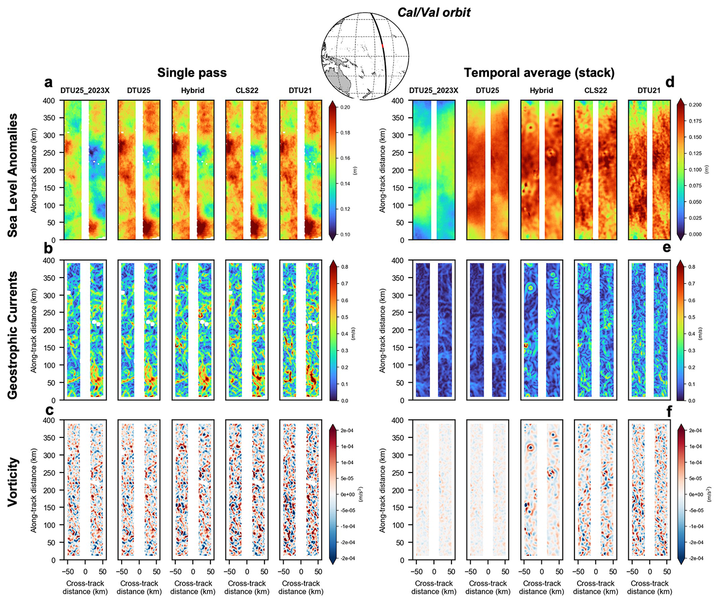
Figure 18 Three oceanographic variables (sea level anomaly a, d, geostrophic currents b, e, and vorticity c, f) computed for a single SWOT pass from the Cal/Val orbit (left, cycle 475 pass 2) and from the temporal average of 90 cycles (right) with different MSS models as reference.

5 Current limitations and future outlook

While the SWOT mission provides groundbreaking new data, this in turn means data processing techniques might not fully encapsulate the newly resolved spectral regimes or current methodologies might not utilize this data to its optimal capability, as opposed to the “mature” nadir satellite altimetry (Abdalla et al., 2021). This paper is our best efforts to utilize the data from SWOT to improve the MSS for SWOT as well as for other users. However as the scientific community gets more familiar with the data, improvements and following revisions are expected. Some of the known deficiencies or expected improvements are described here.

The SWOT data product used to produce the MSS is the v2.0.1 for the 2 km product, and the v1.0.2 for the 250 m product (AVISO/DUACS, 2025a, c). New versions with updated processing and higher data quality is produced periodically, and will in turn improve the quality of the derived MSS. Some known challenges include constrained correction models used to process the SWOT data, such as landmasks, tide models or open ocean/sea ice classification. These lead to either conservative data quality estimates, resulting in potential good data not being included in MSS estimates. Or erroneous corrections applied to the data without quality flagging, which will be included in the MSS and degrade the product.

Due to the scientific community continuously improving either the SWOT data or the corrections used to produce them, reprocessing of the DTU25MSS could be necessary in order to improve the quality of the product. These would appear in the data repository at (Andersen and Nilsson, 2025), with version control and change logs in order to move at the same pace as the scientific community and provide the most up-to-date reference field.

Further studies on the effect on other data sources of including small scale features, such as tidal flats in the MSS, will need to be carried out, to determine the best case for constructing a MSS. While other studies have created time-varying elevation models (Shi et al., 2025), for the DTU25MSS we constrain these effects to the mean of the time period for which we have data available for SWOT. Other areas would be areas with sea ice coverage, as these areas are highly dynamic, and current utilization of SWOT might not reflect the long time average from the full time period.

Future iterations of the MSS would benefit from more regional dependence on the data processing as the regional variation in data processing for the current iteration is kept at a minimum. This was done in order to provide a global good product, but could lead to overconfidence on noisy data in challenging regions or under confidence on good data. Further studies into the regional temporal correlation, short wavelength features, and the correlation features used to grid data is expected to produce an improved product, and utilize the SWOT mission to the full potential.

6 Data availability

The DTU25MSS along with the experimental DTU25MSS_2023X is available at https://doi.org/10.11583/DTU.29412275 (Andersen and Nilsson, 2025) in several data formats and with different reference ellipsoids. Change log is available on the same site.

7 Conclusions

A new global Mean Sea Surface (MSS) is introduced, where we for the first time incorporate wide-swath altimetry from SWOT in order to improve the short wavelengths. The model, DTU25MSS, compensates for the short timescale of SWOT and benefits from the long timescales and large suite of nadir altimeters by building a long wavelength MSS model called the DTU25_LWMSS, to which we constrain all long-wavelengths from SWOT. We then only utilize the short wavelength features from SWOT, and combine these two models to construct the overall MSS model.

Initial inspection and evaluation of the new MSS is carried out, with improvements in the wavelengths below 20 km apparently visible, compared with current state of the art MSS models. Further improvement is seen by incorporating high spatial resolution SWOT data from the 250 m data product in the coastal zone (<40 km from the coast), in order to map complex coastal regions. This is seen to resolve short wavelength features, such as internal lagoons in Atolls or tidal flats. However these small scale features might not correspond to the observations obtained from platforms with large footprints and would need further studies in order to determine the effects of incorporating these into a MSS.

Evaluation with withhold SWOT data from the 3 month Cal/Val orbit is performed, which show improved spatial resolution reaching the limit of upwards continuation (∼30 % improvement) as well as reduction in leakage of omitted geodetic features or noise into oceanographic features from the MSS. However improvement is not global, with data gaps at low and mid latitudes and at high latitudes above the coverage of SWOT (>78°) we keep the DTU21MSS model based on nadir altimetry.

Future iterations of the MSS will benefit from improved SWOT processing, and the improvement of auxiliary corrections SWOT relies on, which in turn will be improved from the utilization of SWOT data. From the results presented here we see a great benefit from utilizing SWOT in improving the marine reference surfaces which will improve the data obtained from SWOT. But the new regime observed from SWOT requires further studies and cross-disciplinary collaboration in the scientific community in order to fully utilize the data and understand the newly resolved features.

Appendix A: Coastal zone mask

A global land mask is available in Fig. A1, to visualize the areas where we use the 250 m SWOT data (green), whereas the majority of the areas we use the 2 km SWOT data or the reference surface, depending on the location (white). The full area shown as green is not based on the 250 m data, but the region wherein the distance from coast data weighting is used (see Fig. 4d), and which is truncated at 40 km distance.

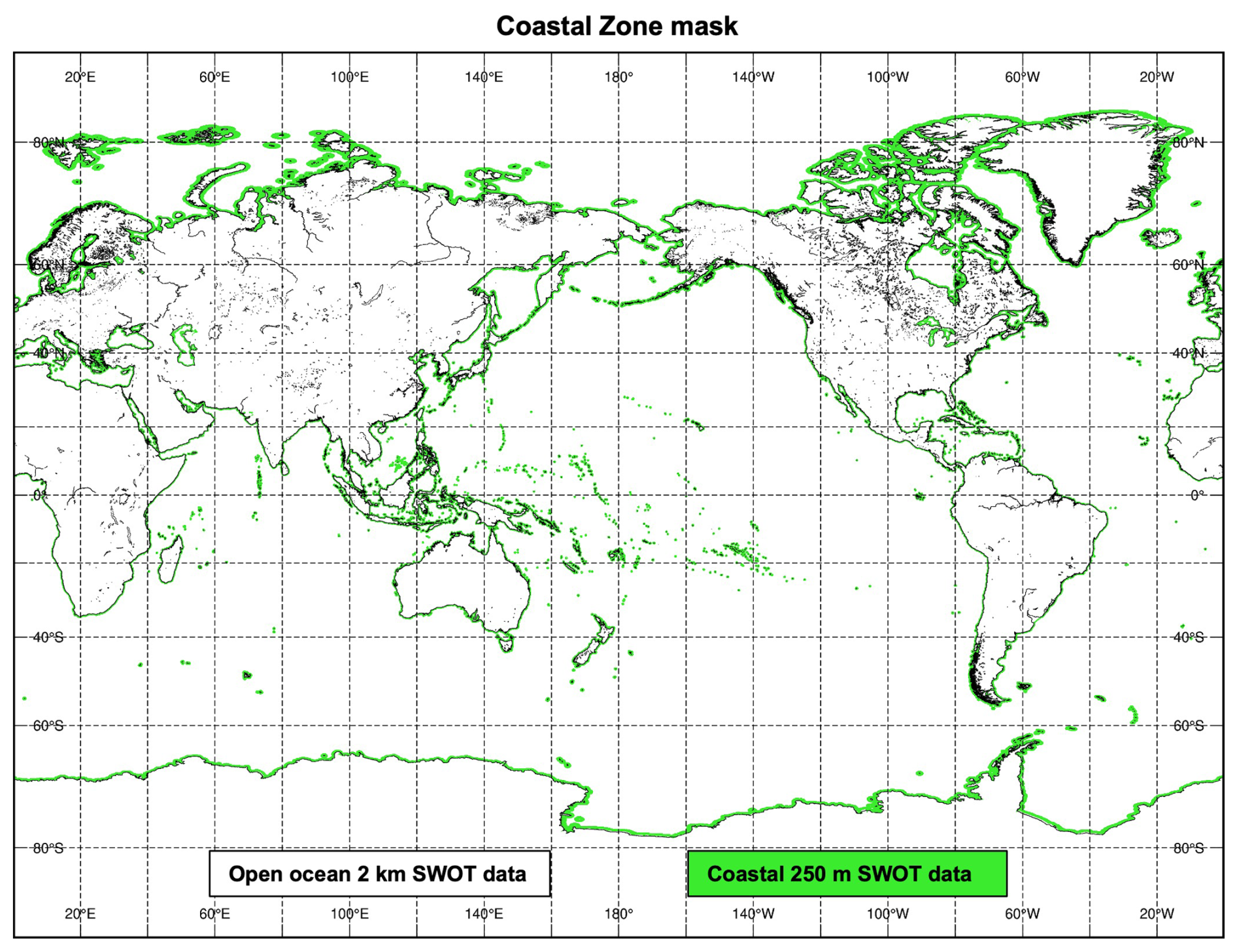
Figure A1 Global map of the 40 km distance from the coast zone where we process the 250 m SWOT data.