Attention enhanced 3D-U-Net+ +  ocean temperature and salinity reconstruction in the northwestern Pacific based on transfer learning

Real-time and accurate three-dimensional ocean temperature–salinity (T–S) field are of great significance for a deeper understanding of ocean dynamics and prediction skill improvement of numerical models. However, current ocean observations, especially those below the sea surface, still suffer from significant limitations in temporal and spatial resolution. Several neural network methods using multi-source satellite data for underwater temperature and salinity reconstruction have been proposed, achieving real-time temperature and salinity reconstruction, but their biases relative to in-situ observations are still significant. This study focuses on the northwestern Pacific region (0–40° N, 120–160° E) and proposes an attention-enhanced three dimensional U-Net$++$ model, which reconstructs daily T–S fields (26 layers, $\mathrm{1}/\mathrm{4}$° resolution, 5–2000 m depth) using real-time available sea surface temperature (SST) and sea surface height (SSH) data. The model introduces cross-scale feature aggregation and selective information gating, allowing it to emphasize temporally coherent surface features most relevant to subsurface variability, while suppressing noise propagation and over-smoothing. By integrating 26 consecutive days of SST and SSH as inputs, the model effectively alleviates the underdetermined problem of mapping limited surface observations to full-depth structures. In addition, a two-stage transfer learning strategy is employed: the model is first pretrained using monthly SST/SSH data and the gridded Argo data to learn observation-dominated low-frequency spatiotemporal patterns, and then fine-tuned using daily SST/SSH data and the high-resolution reanalysis to capture the meso-scale dynamic processes. Evaluation results show that the reconstructed T–S fields agree better with in-situ T–S profiles from World Ocean Database than previous studies, both during the validation period and in long-term statistical analyses, suggesting that the proposed approach is reliable and accurate for subsurface ocean field reconstruction. The reconstructed T–S field is available at https://doi.org/10.57760/sciencedb.31950 (Wang et al., 2025).

1 Introduction

The three-dimensional (3D) temperature and salinity (T–S) fields of the ocean are the most fundamental parameters characterizing the marine environment. Investigations of the three-dimensional T–S fields have provided crucial insights into oceanic dynamical processes, climate variability, and the evolution of marine ecosystems (Curry et al., 2003; Gill, 2016). However, the available in-situ observational data remain extremely sparse in both spatial coverage and temporal resolution (Stewart, 2008), rendering them insufficient for resolving the fine-scale structures and evolution of meso-scale phenomena (Pauthenet et al., 2022). Consequently, the hydrological gridded data reconstructed from these observations also exhibit limited temporal and spatial resolution.

Satellite remote sensing provides global observations of ocean surface parameters (Klemas and Yan, 2014), including sea surface height (SSH), sea surface temperature (SST), and sea surface salinity (SSS), with the advantages of high temporal and spatial resolution. However, these measurements are restricted to the ocean surface and cannot directly capture the subsurface density structure (Talley et al., 2011; Klemas and Yan, 2014). Fortunately, a strong physical coupling exists between the surface and subsurface layers of the ocean. The temperature, salinity, and current structures beneath the surface are closely linked to surface conditions through the exchange of heat and momentum within the seawater (Munk, 1950; Huang, 2010). This intrinsic coupling makes it feasible to reconstruct subsurface T–S fields from surface observations (Fu and Davidson, 1996; Ali et al., 2004; Wu et al., 2012).

Early studies on T–S reconstruction primarily relied on statistical regression (Guinehut et al., 2012), interpolation, or physics-based models (Gilson et al., 1998; Willis et al., 2003). These methods have enabled the estimation of the ocean's vertical structure to some extent. However, the applicability and accuracy are constrained by the discrepancy between the linear assumptions and the inherently nonlinear nature of the real ocean. For instance, reconstruction approaches based on the Surface Quasi-Geostrophic (SQG) approximation assume that surface density variations are entirely governed by temperature (Isern-Fontanet et al., 2006; LaCasce and Mahadevan, 2006), neglecting the influence of salinity and other nonlinear factors. As a result, such methods struggle to accurately represent the complex vertical structures observed in the actual ocean. In recent years, obtaining subsurface temperature and salinity fields through data assimilation has become another important approach (Chen et al., 2025; Martin et al., 2025). On one hand, satellites can provide large-scale and high-frequency sea surface information, and assimilating these observations helps improve the simulation of subsurface temperature and salinity structures (Fu, 2016). On the other hand, existing temperature and salinity observation profiles can be directly used in data assimilation models to further refine the simulated subsurface structures (Bellucci et al., 2007). Although satellite data assimilation has become a major means of obtaining subsurface temperature and salinity fields and has shown good performance in surface and near-surface layers, there remain significant challenges in accurately reproducing the vertical structures of mesoscale eddies (Pilo et al., 2018; Gwyther et al., 2023).

With the rapid development of deep learning, neural networks have demonstrated great potential in the reconstruction of oceanic temperature and salinity fields due to their powerful nonlinear fitting capabilities (Wu et al., 2012; Xie et al., 2025). In recent years, various neural network–based temperature and salinity reconstruction methods have emerged, which can be broadly categorized into four types: point-to-point, surface-to-point, surface-to-surface, and surface-to-volume approaches. Point-to-point methods use sea surface data together with geographical coordinates (latitude and longitude) as network inputs to estimate subsurface temperature and salinity at corresponding locations (Chen et al., 2022). These methods typically adopt architectures such as Long Short-Term Memory (LSTM) or Back Propagation (BP) neural networks (Su et al., 2021; Su et al., 2022; Smith et al., 2023). The surface-to-point approach uses surface data from a small surrounding region to reconstruct the subsurface temperature and salinity at the central point of that region, typically using convolutional neural networks (CNNs) (Zhao et al., 2025). For example, Meng et al. (2021) developed a 2D-CNN and reconstructed subsurface temperature and salinity anomalies (STA, SSA) at the regional center using 20° × 20° patches of Sea level anomaly, sea surface temperature anomaly, sea surface salinity anomaly and wind stress anomaly (SLA, SSTA, SSSA, and WSA). The surface-to-surface approach reconstructs subsurface temperature and salinity fields layer by layer with surface data in a given region (Su et al., 2019), and usually adopts a U-Net architecture (Song et al., 2024; Zhang et al., 2024). The surface-to-volume approach reconstructs three-dimensional subsurface fields (i.e., full-depth temperature and salinity) for a region directly from surface data, typically using neural networks with 3D encoder–decoder architectures (Mao et al., 2023). Notably, this approach involves a mapping from limited input information (surface data) to a much larger output space (multi-depth fields), a process analogous to super-resolution tasks, which remains a considerable challenge.

At present, data-driven neural network reconstruction methods are evolving toward multi-source data fusion. Early studies primarily relied on SST and SSH, whereas later research incorporated additional inputs such as sea surface wind (SSW) and SSS. More recently, studies have even included surface wind stress curl derived from surface wind fields. The inclusion of multiple data sources provides more effective input features, thereby improving reconstruction accuracy (Wu et al., 2012; Cheng et al., 2021; Wang et al., 2021; Yu et al., 2025; Zhao et al., 2025).

However, among current satellite datasets, only SST and SSH are available in real-time, whereas SSW and SSS data exhibit latencies of approximately 1–3 and 3–7 d, respectively. Consequently, to realize real-time reconstruction of subsurface temperature and salinity using neural networks, the input variables are restricted to the real-time accessible SST and SSH. To achieve real-time large-depth reconstruction of subsurface temperature and salinity, this study proposes a method that relies solely on real-time available SST and SSH data. The method is based on an attention-enhanced 3D U-Net$++$ architecture, which effectively captures multi-scale spatial features and deep coupling relationships. A transfer learning strategy introduced by Pan and Yang (2010) is also employed: the network is first pre-trained using monthly SST, SSH, and Argo gridded T–S products to learn real observational information and large-scale temporal patterns; then, it is fine-tuned using daily SST, SSH, and a well-recognized Global Ocean Reanalyses and Simulations Stream 2 version 4 data (GLORYS2V4) to capture daily dynamic processes and characteristics. To address the challenge of reconstructing full-depth fields from limited input data, a long time-series input strategy is introduced, where a sequence of past surface observations is used as input. Results show that this strategy could significantly improve the accuracy of full-depth T–S reconstruction. The study area, spanning 0–40° N and 120–160° E, is a dynamically active region of global significance, strongly influenced by major circulation systems such as the Kuroshio and North Equatorial Current. The model successfully reconstructs temperature and salinity from 5 to 2000 m. Results demonstrate that the model achieves higher reconstruction accuracy than several widely used datasets across both validation and long-term sequences, and shows closer agreement with World Ocean Database (WOD) in-situ T–S profiles. It indicates that the proposed neural network is capable of generating subsurface fields that are consistent with reanalysis data and show superior alignment with observational profiles under surface constraints. Thereby it provides a feasible and efficient framework for the real-time 3D reconstruction of ocean temperature and salinity fields.

The remainder of this paper is organized as follows: Sect. 2 presents the data and methods used in this study. The data section introduces the neural network training data employed in this work and the comparative data used for quality analysis. The methods section provides a detailed description of the attention-enhanced 3D U-Net$++$ model, the transfer learning training strategy, and the approach of using long-term time series of sea surface data as network inputs. Section 3 presents the results and analysis, including comparative analyses of different transfer learning training strategies, the impact of using long-term time series of sea surface data as network inputs on reconstruction results, and the reliability analysis of the model-reconstructed temperature and salinity data. Section 4 concludes the paper.

2 Data and Methods

2.1 Data

2.1.1 Training Data

The SST data used in this study were obtained from the Optimum Interpolation Sea Surface Temperature (OISST) dataset provided by the National Oceanic and Atmospheric Administration (NOAA) (Huang et al., 2021). This dataset has a global spatial resolution of 0.25° × 0.25° and a daily temporal resolution. It integrates satellite observations from multiple platforms with various in situ measurements. The dataset is publicly available at: https://www.ncei.noaa.gov/data/sea-surface-temperature-optimum-interpolation/v2.1/access/avhrr/ (last access: 29 June 2026).

The SSH data were provided by the Archiving, Validation, and Interpretation of Satellite Oceanographic Data (AVISO) program. This dataset is derived from the integration of multiple satellite altimeter missions, which have undergone rigorous calibration, validation, and data assimilation processes. It provides a spatial resolution of $\mathrm{1}/\mathrm{8}$° and a daily temporal resolution. The dataset can be accessed at: https://doi.org/10.48670/moi-00148 (AVISO+, 2026).

During the pretraining stage of the neural network, the gridded Argo product developed by the International Pacific Research Center (IPRC) was used as the target data. This dataset was generated through a variational interpolation algorithm applied to Argo float observations, with a spatial resolution of 1° × 1° and a monthly temporal resolution. It is available at: https://apdrc.soest.hawaii.edu/projects/Argo/data/gridded/On_standard_levels/index-1.html (last access: 29 June 2026).

For the fine-tuning stage, daily temperature and salinity fields from the GLORYS2V4 reanalysis dataset were employed as the ground truth. The GLORYS2V4 dataset provides global ocean reanalysis fields on a 0.25° grid by assimilating observational data into an ocean circulation model. It enables comprehensive analysis of ocean dynamics and contributes to improved weather and climate predictions. The dataset is available at: https://doi.org/10.48670/moi-00024 (GLORYS2V4, 2026).

2.1.2 Validation data

To objectively assess the reliability of the reconstructed products, this study employed quality-controlled T–S profiles from the WOD for error analysis (Mishonov et al., 2024). The profiles provided by the XBT have been used after correction (Cheng et al., 2014). The WOD dataset is publicly available at: https://www.ncei.noaa.gov/products/world-ocean-database (last access: 29 June 2026).

The High-Resolution Northwest Pacific Temperature Salinity Current Dataset was also utilized. This dataset integrates historical hydrographic observations from CTD and Argo floats with recent satellite altimeter data. It is derived using the Height Geostrophic Empirical Mode (HGEM) method (Zhang and Sun, 2012), which reconstructs three-dimensional ocean temperature, salinity, and velocity fields based on large-scale continuous satellite altimetry observations. The dataset has a spatial resolution of 0.25° × 0.25° and a temporal resolution of one week. It is available at: https://msdc.qdio.ac.cn/data/metadata-special-detail?id=1456480706929647617&otherId=1456480709660139521 (last access: 29 June 2026).

The China Global Ocean Fusion Dataset 1.0 (CGOF1.0) was also adopted for comparative analysis. This dataset extensively integrates more than 40 publicly available global ocean environmental datasets together with China's officially released ocean data. It employs a data–physics hybrid intelligent big data methodology and a sparse observation data migration and reconstruction technique. The dataset has a spatial resolution of $\mathrm{1}/\mathrm{12}$° and a temporal resolution of one month. It can be accessed at https://www.cmoc-china.cn/pages/CGOF.html (last access: 29 June 2026).

The global reanalysis product from the Hybrid Coordinate Ocean Model (HYCOM) was also utilized in this study. This system employs the Navy Coupled Ocean Data Assimilation (NCODA) scheme to assimilate available satellite altimeter observations, sea surface temperature, and in-situ vertical temperature and salinity profiles. HYCOM utilizes a unique hybrid coordinate system that transitions between isopycnal coordinates in the open ocean, z-level coordinates in the mixed layer, and sigma coordinates in shallow coastal regions. The dataset typically features a spatial resolution of $\mathrm{1}/\mathrm{12}$° and a temporal resolution of one day. It is accessible at: https://www.hycom.org/dataserver (last access: 29 June 2026).

The Ocean Reanalysis System 5 (ORAS5) produced by the European Centre for Medium-Range Weather Forecasts (ECMWF) was introduced for comparative analysis. Based on the NEMO ocean model coupled with the LIM2 sea-ice model, it utilizes the NEMOVAR variational data assimilation methodology to integrate extensive in-situ and satellite observations. ORAS5 provides a consistent historical reconstruction of the ocean state with a spatial resolution of 0.25° and a temporal resolution of one day. The dataset can be accessed at: https://www.ecmwf.int/en/forecasts/dataset/ocean-reanalysis-system-5 (last access: 29 June 2026).

2.2 Methods

2.2.1 3D-UNet$++$

The U-Net$++$ architecture used in this study is a deep learning network originally designed for image segmentation tasks. It was proposed as an enhanced version of U-Net (Zhou et al., 2018). Its structure is illustrated in Fig. 1. U-Net$++$ employs an encoder–decoder architecture with deep supervision and a series of dense skip connections between the encoder and decoder. Convolutional layers are introduced along the skip pathways to reduce the semantic gap between feature maps of the encoder and decoder. The dense skip connections play a pivotal role in bridging the semantic gap between the encoder and decoder feature maps. Unlike the simple long skip connections in the standard U-Net, these nested, dense pathways pass feature maps through a series of convolutional blocks before fusing them with the decoder. This process gradually aggregates features at varying semantic levels, ensuring that the decoder receives more semantically rich and consistent information. Consequently, this mechanism allows the network to capture complex multi-scale features more effectively – acting essentially as an ensemble of U-Nets – which significantly improves gradient flow during training and enhances segmentation accuracy for objects of diverse sizes.

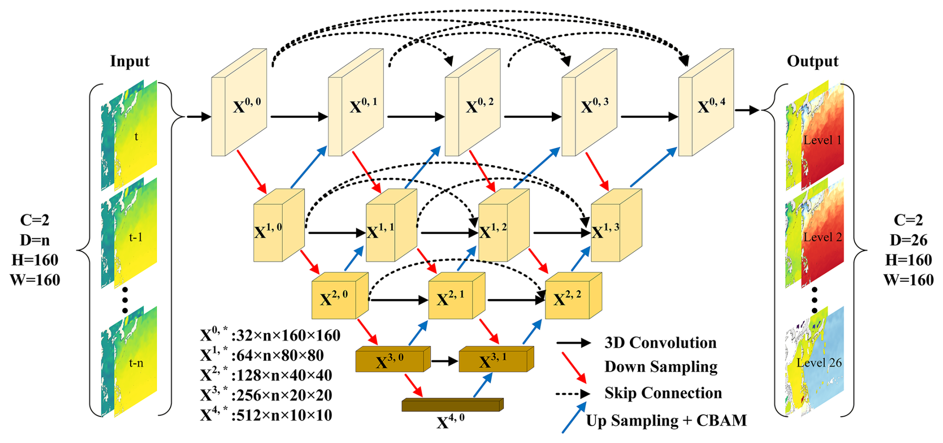
Figure 1 Schematic diagram of the 3D-U-Net$++$ neural network structure, where X^i,j represents the feature map at level i and stage j.

The deep supervision mechanism in U-Net$++$ can operate in two modes: precise and fast. In the precise mode, outputs from all sub-branches are averaged to generate the final segmentation map, while in the fast mode, only one segmentation branch is used, which also allows for model pruning. By performing multi-level feature fusion, U-Net$++$ effectively utilizes hierarchical feature information, transmitting low-level details to high-level semantic representations, thereby improving both the accuracy and boundary sharpness of the reconstruction results.

The 3D-U-Net$++$ network employed in this study is derived from the conventional U-Net$++$ architecture by replacing all 2D operations – such as convolution, pooling, and up-sampling – with their 3D counterparts. Notably, 3D convolution is capable of simultaneously processing data across four dimensions: depth, channel, height, and width (Tran et al., 2015). This capability renders the network highly suitable for physical oceanographic datasets, which typically encompass spatial extent, depth, and temporal information.

Building on this foundation, to further enhance the model's capability in handling the complex task of temperature–salinity reconstruction and to improve its ability to capture the importance of different local and channel-wise features, a Convolutional Block Attention Module (CBAM) was integrated into the network. The architecture of CBAM is shown in Fig. 2a. CBAM aims to strengthen the representational power of convolutional neural networks by focusing on the most relevant features across both spatial and channel dimensions (Woo et al., 2018). By combining channel attention and spatial attention, CBAM provides a more comprehensive and effective feature extraction mechanism, thereby improving the representational capability of the 3D U-Net$++$. CBAM consists of two main components: the Channel Attention Module (CAM) and the Spatial Attention Module (SAM), whose structures are illustrated in Fig. 2b and c, respectively.

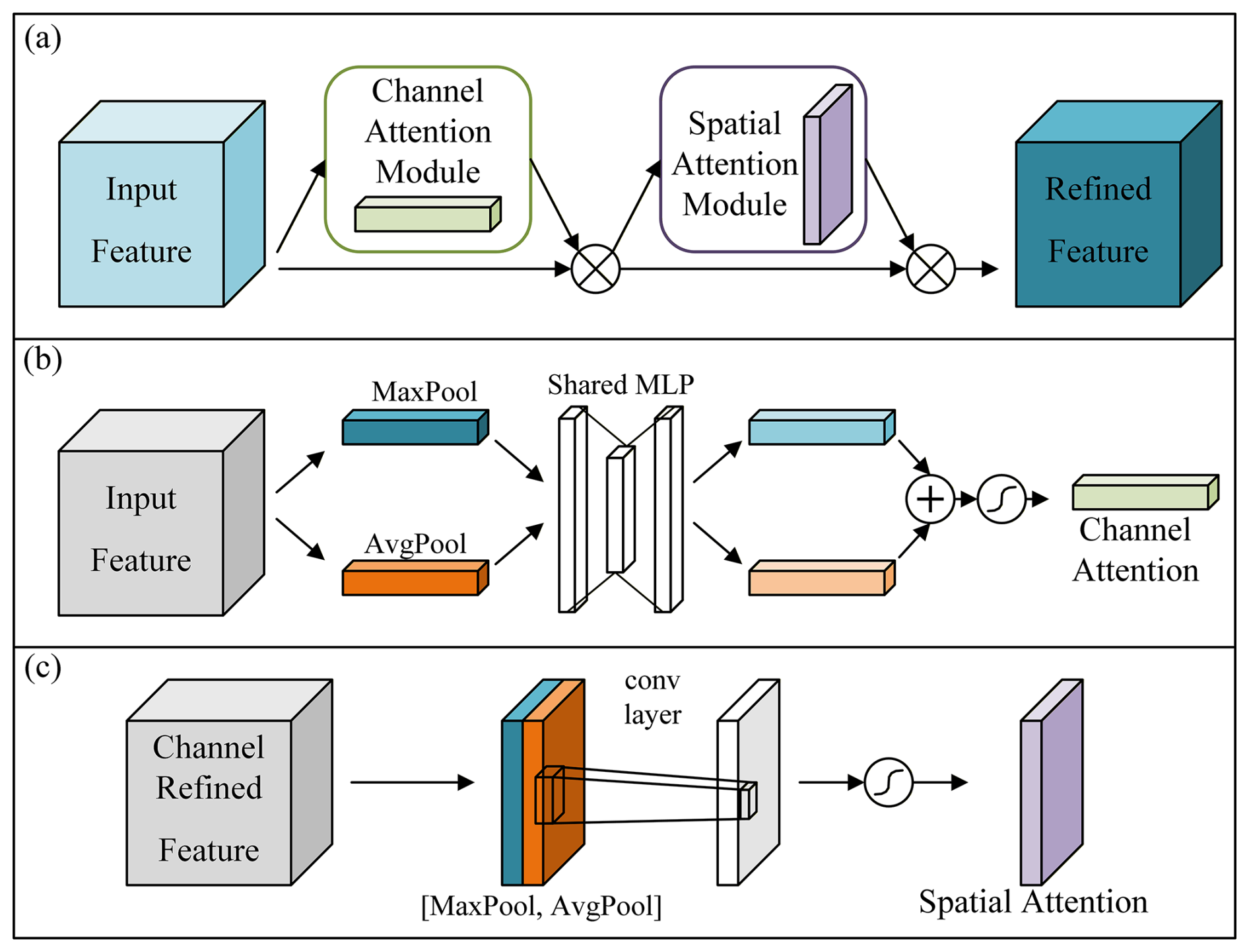
Figure 2 (a) Network structure diagram of CBAM. (b) CAM branch in CBAM. (c) SAM branch in CBAM.

As illustrated in Fig. 1, the neural network is designed to directly accept a 4D tensor with a shape of (C × D × H × W) as input. In this study, C is set to 2, representing the two input channels: SSH and SST. D is set to 26, denoting the continuous time series of sea surface data from the past 26 d (details regarding D are provided in Sect. 2.2.3). H and W are both set to 160, corresponding to the spatial dimensions of the study area. The output dimensions of the network are (2, 26, 160, 160). Specifically, the first dimension 2 represents the two target variables: seawater temperature and salinity; 26 corresponds to 26 depth levels spanning from 0 to 2000 m; and 160 represents the spatial dimensions of the study area. Within the network architecture, down-sampling is performed using 3D max pooling, while up-sampling is achieved via 3D transposed convolution.

The CAM operates by learning which channels in the feature maps are more important, thereby enhancing the most informative channels while suppressing irrelevant ones. Specifically, the module first aggregates spatial information via global average and max pooling. It then applies a shared multi-layer perceptron (MLP) to generate channel-wise attention. The computational process of this module can be expressed as follows:

$$\begin{array}{}\text{(1)}& M_{\mathrm{c}}\left(F\right)=\mathit{\sigma }\left(\mathrm{MLP}\left(\mathrm{AvgPool}\left(F\right)\right)+\mathrm{MLP}\left(\mathrm{MaxPool}\left(F\right)\right)\right)\end{array}$$

where M_c(F) is output of the CAM, σ() represents the sigmoid activation function, MLP() represents the multilayer perceptron, AvgPool() and MaxPool() represent mean pooling and max pooling, respectively. F is the input feature.

The SAM focuses on the spatial locations of features, learning where the most important regions lie within the spatial domain. It first applies global average pooling and max pooling along the channel dimension, concatenates the resulting feature maps, and then performs a convolution operation to generate a spatial attention map that highlights key spatial areas. The computational process of SAM can be expressed as follows:

$$\begin{array}{}\text{(2)}& M_{\mathrm{s}}\left(F\right)=\mathit{\sigma }\left(f^{\mathrm{7}\times \mathrm{7}}\right(\left[\mathrm{AvgPool}\right(F);\mathrm{MaxPool}(F\left)\right]\left)\right)\end{array}$$

where M_s(F) is output of the CAM, σ() represents the sigmoid activation function, $f^{\mathrm{7}\times \mathrm{7}\times \mathrm{7}}\left(\right)$ denotes a 3D convolution operation with a kernel size of 7 × 7 × 7, AvgPool() and MaxPool() represent 3D mean pooling and 3D max pooling, respectively. F is the input feature.

Together, CAM and SAM enable the CBAM to selectively emphasize informative features, reduce irrelevant information, and enhance the discriminative capability of the model. Consequently, CBAM improves model performance across various tasks such as classification, detection, and segmentation.

2.2.2 Transfer Learning

To enhance the generalization capability of the model and enable it to extract features across different data modalities, thereby learning the common characteristics shared by observational and reanalysis datasets, this study employed a transfer learning strategy during neural network training.

Transfer learning is a paradigm in machine learning whose fundamental concept is to transfer knowledge acquired from one task (the source domain) to improve learning performance on another related task (the target domain) (Pan and Yang, 2010). The transfer learning framework adopted in this study is illustrated in Fig. 3.

Figure 3 Overview of Transfer Learning Strategies.

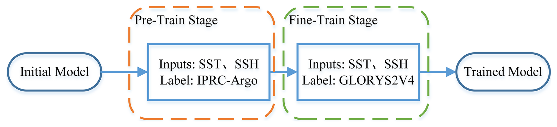
In this study, model training was conducted in two distinct stages. During the pretraining stage, monthly mean SST and SSH fields were used as input data, while the IPRC-Argo gridded temperature and salinity products served as the target labels. In the retraining (fine-tuning) stage, daily SST and SSH data were used as inputs, and the GLORYS reanalysis dataset was adopted as the target.

It is worth noting that due to differences in the temporal and spatial resolutions of the label data used in the two stages of transfer learning, the datasets were unified for this study. The specific data processing methods are detailed in Table 1.

Table 1 Data processing and normalization methods.

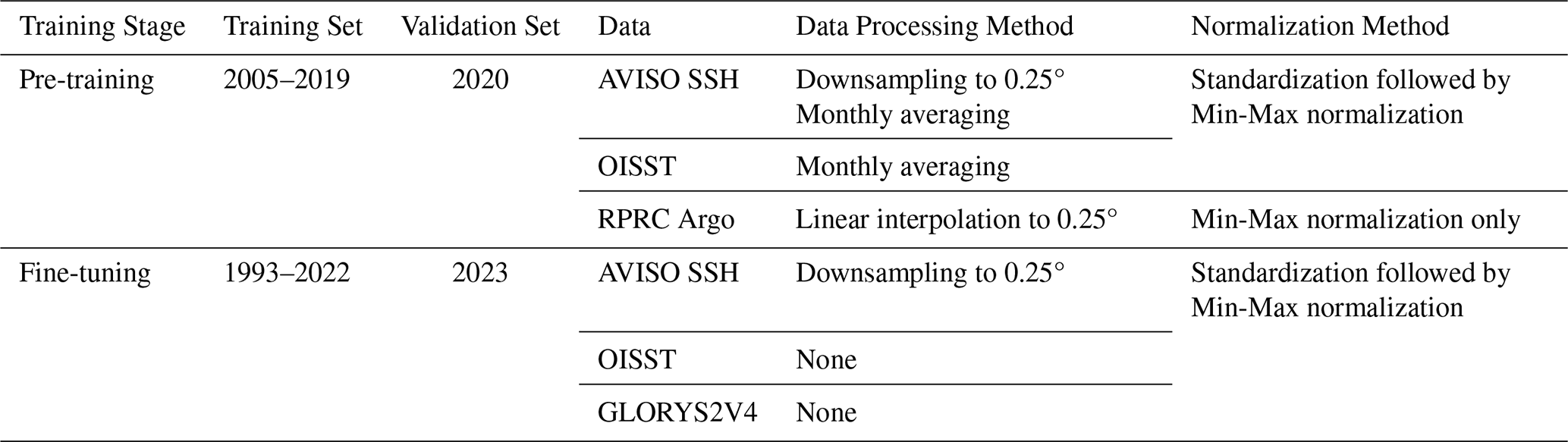
In the pre-training phase, the input data were averaged monthly to match the temporal resolution of the IPRC Argo temperature and salinity data. Additionally, to be consistent with the OISST data and match the output dimensions of the neural network, both the $\mathrm{1}/\mathrm{8}$° resolution AVISO SSH data and the IPRC Argo data were linearly interpolated to 0.25°. In the fine-tuning phase, since both the training data and label data are daily records, no temporal averaging was performed; however, the $\mathrm{1}/\mathrm{8}$° AVISO SSH data were down-sampled to 0.25°.

Furthermore, the data normalization strategies differed between the two stages. As the pre-training data predominantly contain monthly signals, the label data were simply normalized to the range of [0, 1]. In contrast, for the fine-tuning phase – where the objective was for the network to learn smaller time-scale signals (i.e., abrupt changes) based on the pre-trained model – the label data were first standardized using the mean and standard deviation, and then normalized to [0, 1]. To ensure consistency, the input data for both stages were processed using the same two-step approach: standardization followed by [0, 1] normalization.

During the pre-training stage, the network learns the real observations contained in the IPRC Argo data, the large-scale statistical relationships between monthly SST/SSH and three-dimensional T–S fields, as well as the oceanic background state, seasonal variability, vertical structure, and low-frequency spatial correlations. This provides a more physically meaningful initialization of the neural network weights. During the fine-tuning stage, the network inherits the weights learned after pre-training. Building on this foundation, continued training with daily-resolution data enables the network to focus more specifically on capturing and reconstructing transient mesoscale dynamical processes from daily data, thereby improving its ability to fit small-scale signals and enhancing training convergence efficiency.

2.2.3 Long-Term Sea Surface Time-Series as Input for Model Training

This study aims to achieve high-accuracy reconstruction of subsurface temperature and salinity across 26 depth layers (5–2000 m) using a neural network. The input data include SST and SSH, while the outputs are multi-level subsurface temperature and salinity profiles.

The main challenge of this task lies in the fact that traditional methods typically rely only on single-time (t) sea surface observations to infer the corresponding three-dimensional temperature–salinity structures, as shown in Fig. 4a. Because the input feature dimension is relatively low while the output space is high-dimensional, the model must recover complex vertical structures from limited surface information. This imposes strict demands on the network's ability to capture and generalize spatial–temporal relationships. In essence, this problem is analogous to super-resolution reconstruction, characterized by information insufficiency and non-uniqueness.

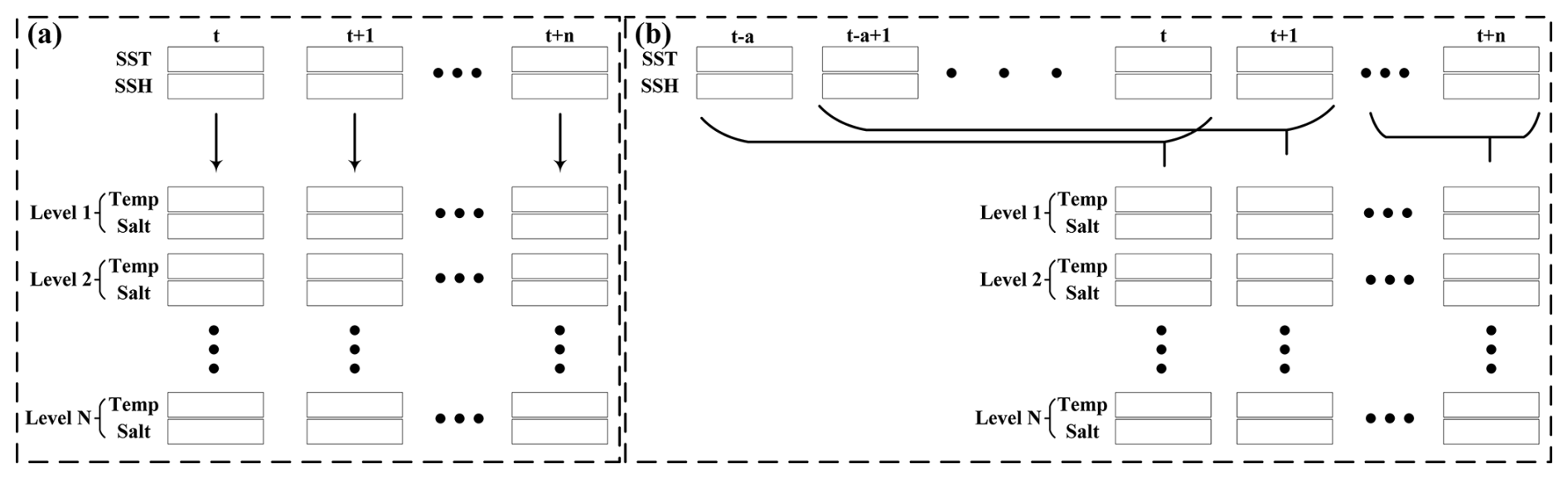
Figure 4 Two different data input approaches. (a) Temperature and salinity reconstruction using single-day sea surface data, where n denotes the total time length and t represents the time step. (b) Temperature and salinity reconstruction using consecutive multi-day sea surface data, where n denotes the total time length, t represents the time step and a represents the time window length.

To address this limitation, we introduce an improved strategy that incorporates temporal sequence information. Specifically, the network input is extended from a single-time snapshot to a continuous days sequence of surface observations, spanning from t−a to t, as show in Fig. 4b. This design leverages the temporal evolution of oceanic processes, enabling the network to learn the dynamic relationships governing subsurface thermal and haline structures.

3 Result

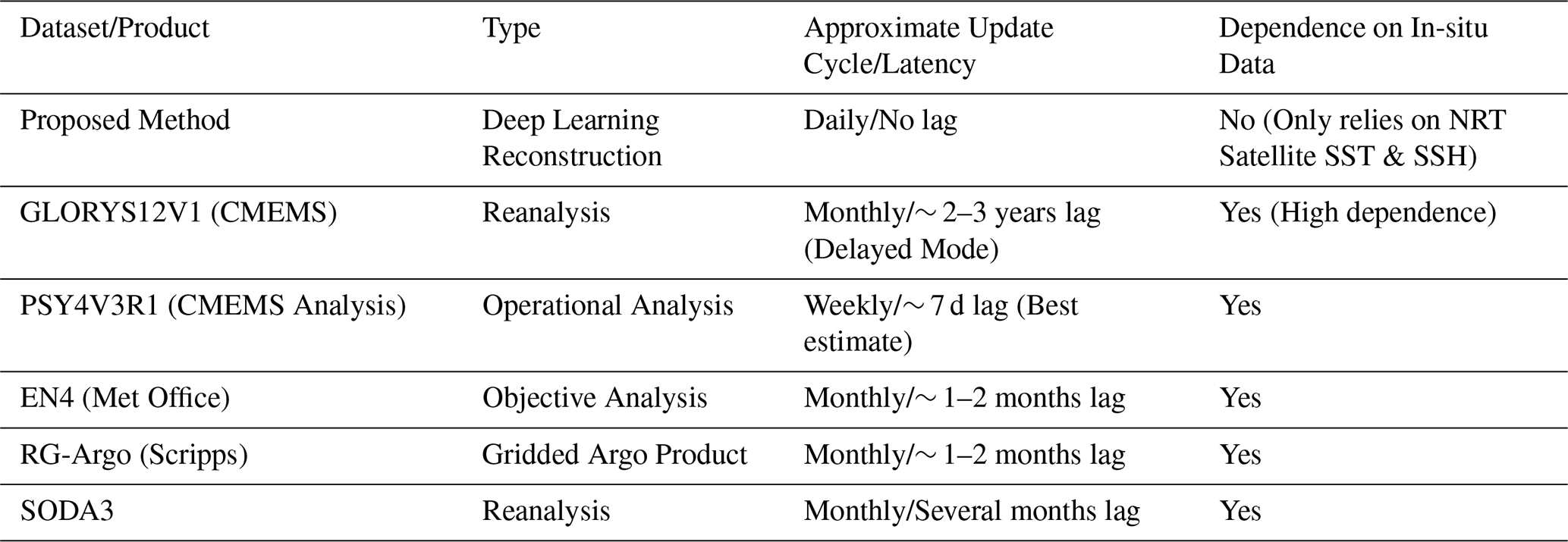
Model training and inference were conducted on a supercomputing cluster equipped with an Intel^® Xeon^® Gold 5218R CPU and an NVIDIA A100-PCIE-40GB GPU. The average inference time required to generate daily 3D T–S fields for the entire region is approximately 5 s. In contrast to traditional reanalysis products (e.g., GLORYS and EN4) which typically suffer from latencies ranging from weeks to months due to the assimilation of sparse in-situ data (see Table 2), our method relies exclusively on real-time satellite observations, enabling real-time reconstruction using data from the current day.

Table 2 Comparison of update cycles and approximate time lag (latency) between the proposed method and mainstream products.

3.1 Transfer Learning

To identify the optimal transfer learning approach, multiple transfer learning strategies were tested by conducting comparative experiments in this study. These included freezing only the encoder, freezing only the decoder, and freezing network weights at different percentage positions from the input to the output layers. In the comparative experiments, inputs spanning multiple months and multiple days were employed for the pre-training and fine-tuning stages, respectively. The pre-training phase utilizes data from the preceding a consecutive months, whereas the fine-tuning phase employs data from the preceding a consecutive days (refer to Sect. 3.2 for the specific value of a). In this experiment, the value of a is set identically in both the pre-training and fine-tuning stages. Although the temporal resolutions of the data used in the two stages differ, the network does not contain any explicit temporal memory structure. Instead, it processes only time-ordered stacked inputs, with the core objective of learning the variation patterns within the stacked sequence rather than fixed monthly or daily labels. The 3D U-Net$++$ and attention modules are mainly responsible for extracting features from the stacked data, and thus their spatial feature extraction capability can be reused across different time scales, while fine-tuning is required to adapt to changes in frequency. Although the two stages share the same input variables, they differ in temporal sampling frequency and target information content. The pretraining stage emphasizes low-frequency, observationally constrained background structures, whereas the fine-tuning stage captures higher-frequency variability and reanalysis-consistent dynamics. Therefore, the transfer primarily concerns the reuse of spatially meaningful feature representations and physically plausible parameter initialization, while temporal scale-specific adaptation is performed during global fine-tuning.

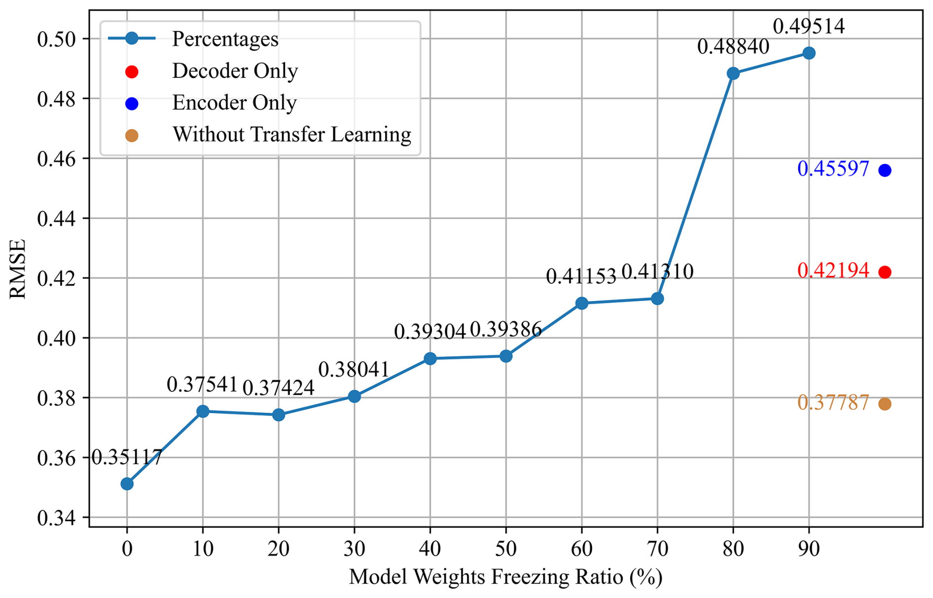
Figure 5 Average RMSE between model outputs and WOD T–S profiles data during 2023 under different transfer learning strategies.

As illustrated in Fig. 5, the comparative results indicate that the reconstruction performance of the neural network varies across different transfer learning strategies. When the model was trained solely on the GLORYS2V4 reanalysis data without transfer learning, the baseline RMSE was 0.3779, which is comparable to the RMSE between the 2023 GLORYS T–S data and the WOD T–S profiles (see Sect. 3.3.2). This suggests that, when trained only on GLORYS2V4 data, the network can achieve an overall accuracy close to that of GLORYS itself within the evaluated observations.

When transfer learning was applied by freezing the encoder, the RMSE increased to 0.4560, whereas freezing the decoder produced a lower RMSE of 0.4219. Further analysis of gradually freezing network layers from the input to the output revealed a non-monotonic pattern. The lowest RMSE of 0.3512 was obtained when no layers were frozen, suggesting that full adaptability during fine-tuning is beneficial for this task. When 10 %–30 % of the network was frozen, the model achieved relatively good performance, with RMSE values close to the baseline. However, when more than half of the network parameters were frozen, the RMSE increased markedly.

These results suggest that global fine-tuning, rather than partial freezing, is the most suitable transfer learning strategy under the present data conditions. Given the differences in temporal scale, label characteristics, and information density between the pre-training and fine-tuning stages, freezing part of the parameters may limit the model's ability to adapt to the higher-frequency daily-scale features. Therefore, full fine-tuning appears to be more effective than partial freezing. This does not necessarily imply that transfer learning directly provides reusable high-level features; rather, it suggests that transfer learning mainly offers a physically constrained parameter initialization that facilitates subsequent adaptation. From an oceanographic perspective, the transfer process can be interpreted as a background-to-perturbation learning paradigm. During pre-training with monthly, coarse-resolution IPRC Argo data, the network learns large-scale climatological background information, including basic stratification, seasonal cycles, and global vertical covariance structures. This initialization places the model in a physically plausible region of the high-dimensional optimization landscape. During fine-tuning with daily, high-resolution GLORYS data, global fine-tuning allows the network to focus on capturing higher-frequency synoptic-scale variability, such as mesoscale eddies and fronts perturbing the pre-established background state.

In summary, because the network is fine-tuned on GLORYS2V4 data, the discrepancy between the reconstructed fields and the WOD observational profiles can be expected to approach, but not necessarily equal, the discrepancy between the GLORYS2V4 labels and the WOD profiles. Initializing the network with the IPRC Argo dataset helps the model retain physically meaningful information while establishing a monthly-scale representation of the ocean background. Building on this foundation, the fine-tuning stage enables the network to learn the dynamic mapping relationships and shorter-time-scale signals present in the GLORYS2V4 data. Validation against WOD profile data indicates that this transfer learning strategy preserves consistency with GLORYS2V4 while also improving agreement with the available WOD observations within the evaluated depths and regions.

In this study, we therefore adopted a transfer learning strategy without weight freezing, in which the model was pre-trained on IPRC Argo data and then fine-tuned on GLORYS2V4 data.

3.2 Input Time Series Data

To determine an appropriate input sequence length for the network, an ablation study was conducted. Considering computational cost, input time series lengths of 1, 4, 8, 10, 20, 26, 30, and 40 d were evaluated. The experimental results are shown in Fig. 6 and suggest a negative relationship between input sequence length and reconstruction error. As the time step increases from 1 to 20 d, the RMSE for both variables decreases noticeably – Temperature RMSE decreases from 0.63563 to 0.61222 °C, and Salinity RMSE decreases from 0.09874 to 0.09475 PSU. This suggests that incorporating historical surface data may help reduce the ambiguity associated with the super-resolution task. In addition, continuous sea surface time series may provide useful physical constraints for reconstructing underwater 3D T–S fields, which may improve reconstruction accuracy within the evaluated setting.

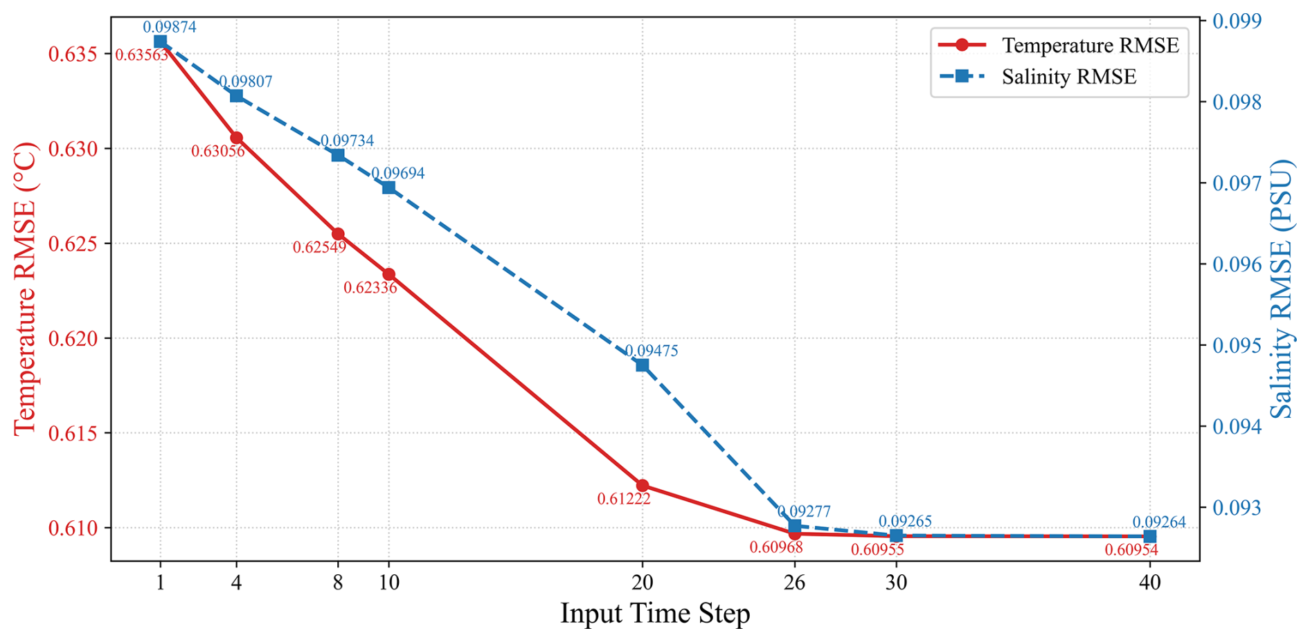
Figure 6 RMSE between the reconstructed data and WOD profiles under different input time series lengths in 2023.

Notably, the performance gain begins to saturate beyond an input length of 26 d. Between time steps 30 and 40, the RMSE curves for both temperature and salinity plateau (stabilizing around 0.6095 °C and 0.0926 PSU, respectively). To balance computational cost and accuracy, the time series length of the input data was set to 26 in this study.

3.3 Model Performance

3.3.1 Comparison of the Model Reconstructions with GLORYS2V4

Figures 7 and 8 respectively present the vertical profiles of RMSE and correlation coefficients for temperature and salinity, with curves for different months illustrating seasonal variations and vertical characteristics.

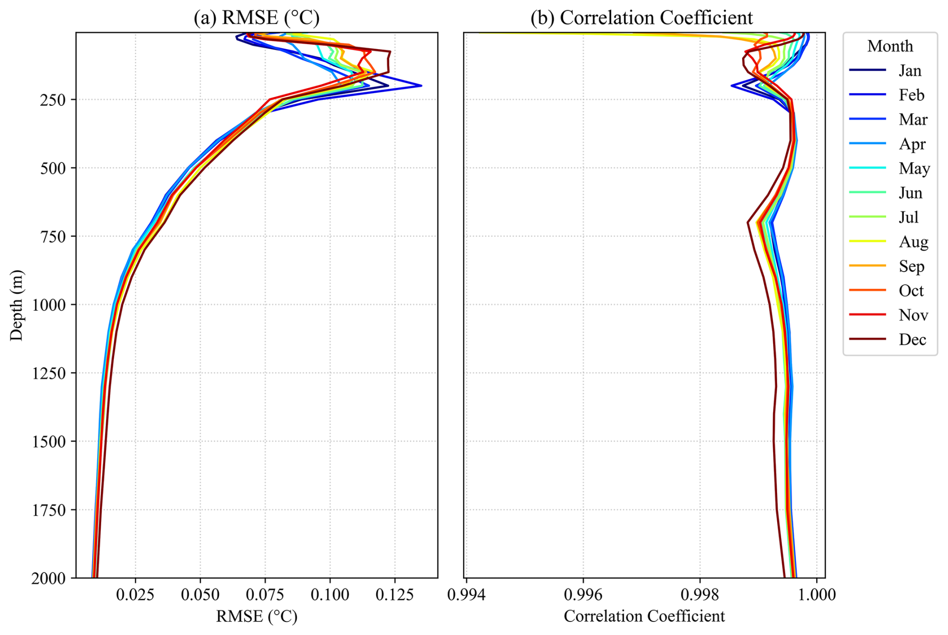
Figure 7 (a) RMSE and (b) correlation coefficient between the model-reconstructed temperature fields and the GLORYS2V4 temperature data in 2023.

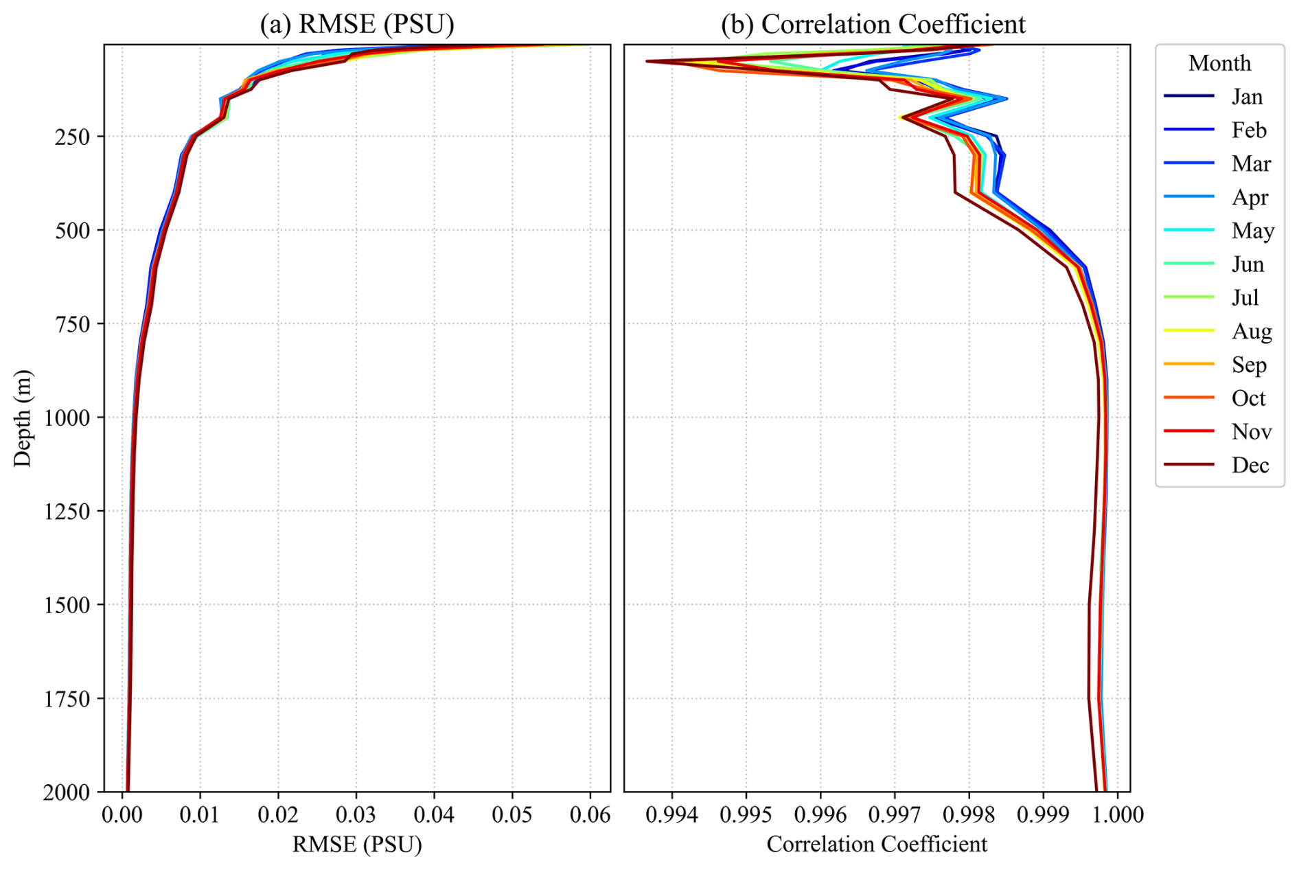
Figure 8 (a) RMSE and (b) correlation coefficient between the model-reconstructed salinity fields and the GLORYS2V4 salinity data in 2023.

From the RMSE distribution of temperature reconstruction (Fig. 7a), the overall RMSE ranges between 0.025 and 0.125 °C. Above 250 m, the temperature RMSE increases with depth, while below 250 m it gradually decreases and becomes relatively low at depths greater than 1000 m, where it remains around 0.015 °C. This pattern suggests that the neural network can capture the relatively stable structure of deep-sea temperatures, although some deviations remain in the subsurface layers influenced by atmospheric forcing and mixed-layer dynamics. The correlation coefficients (Fig. 7b) remain above 0.99 across all depths, indicating strong consistency and suggesting that the model preserves the linear response relationship of temperature variations reasonably well.

The reconstructed salinity RMSE (Fig. 8a) generally decreases with depth, with surface RMSE values ranging from 0.02 to 0.06 PSU. In deeper layers (> 1000 m), the RMSE decreases markedly and approaches 0 PSU, suggesting that the model reproduces the salinity structure in deep ocean regions with good agreement. The overall correlation coefficients remain above 0.99 (Fig. 8b), with slight fluctuations in the upper layers but limited variation among months, which suggests that the model captures the spatiotemporal distribution patterns of salinity reasonably well.

As shown in Figs. 9 and 10, the reconstructed temperature and salinity fields exhibit spatial patterns that are highly similar to those of the GLORYS2V4 data, reproducing the latitudinal gradients and large-scale thermohaline structures reasonably well. The error maps suggest that the discrepancies are generally limited and fairly uniform across the study region, with no obvious areas of concentrated error and near-zero differences in most regions. At greater depths, such as 800 and 1000 m, the errors decrease further and no clear systematic bias is observed, suggesting improved stability and reliability of the model in deep-ocean environments.

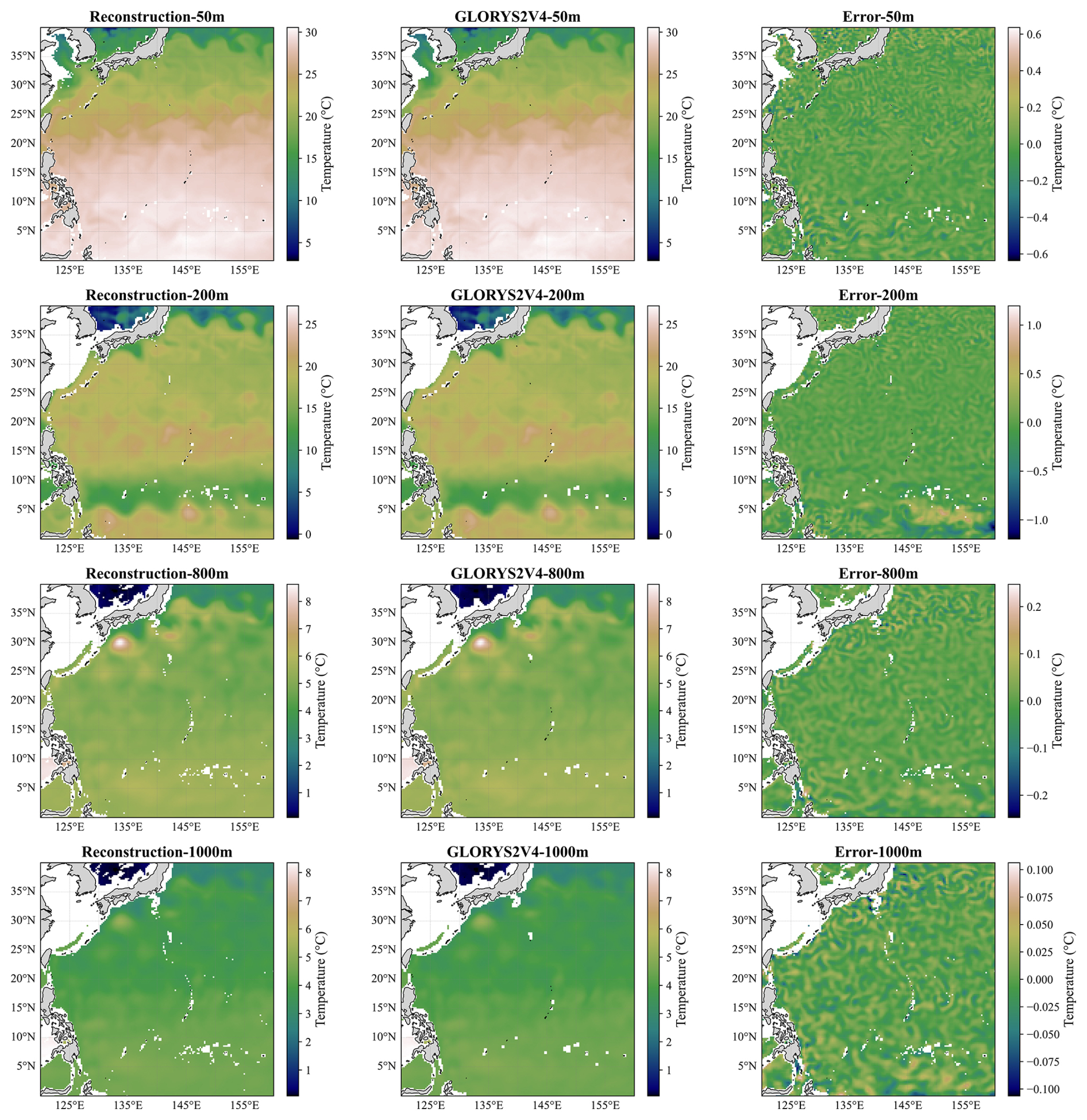
Figure 9 Reconstructed temperature (left) and GLORYS2V4 temperature (middle) and their differences (right) at depths of 50, 200, 800, and 1000 m on 1 January 2023.

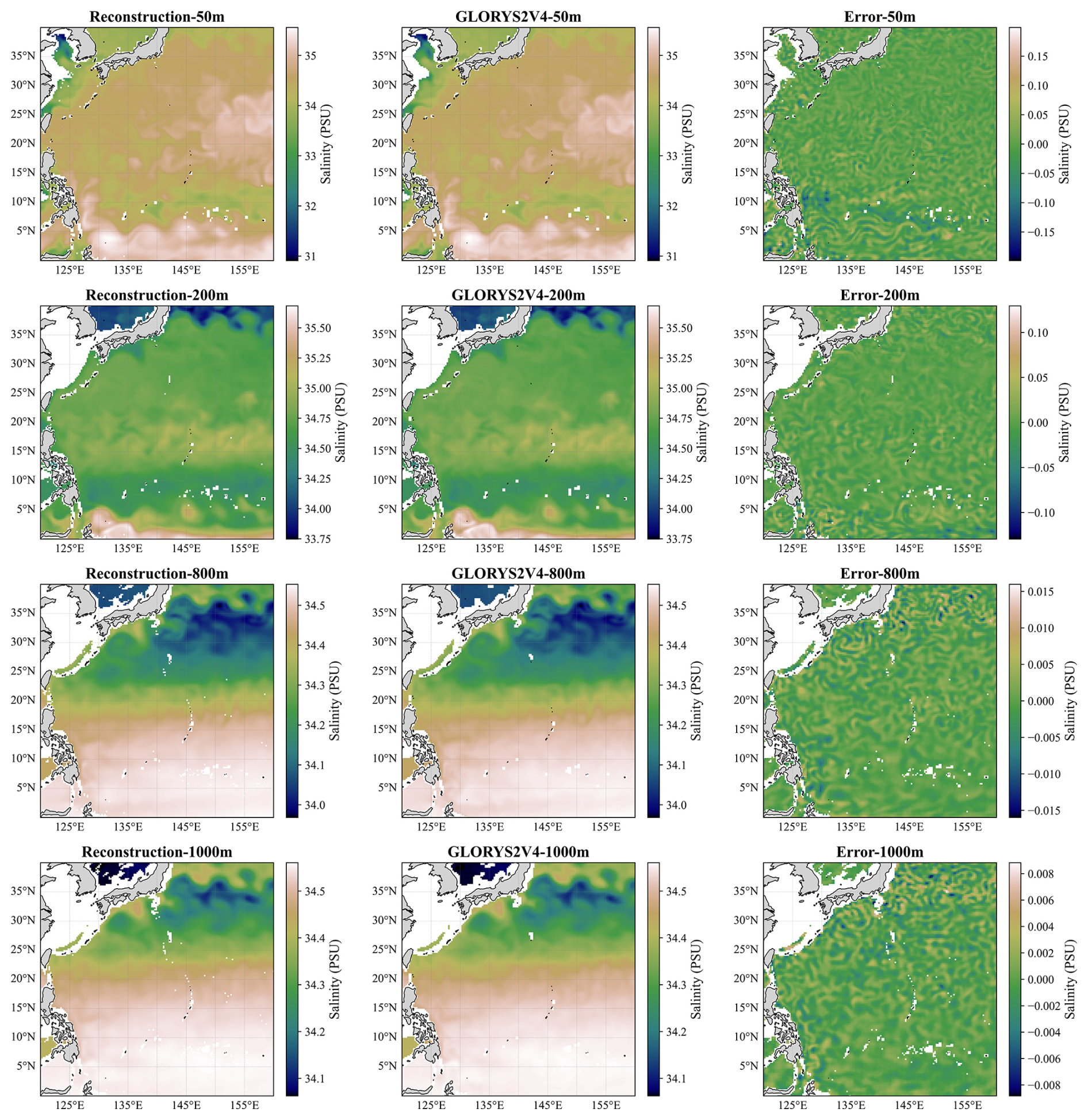
Figure 10 Reconstructed salinity (left) and GLORYS2V4 salinity (middle) and their differences (right) at depths of 50, 200, 800, and 1000 m on 1 January 2023.

Figure 11 shows the spatial distribution of RMSE at different depths throughout the validation period. At depths of 50 and 200 m, the RMSE of the validation set is mainly concentrated in the North Equatorial Countercurrent (NECC) region. In contrast, at 800 and 1000 m, the RMSE is concentrated primarily in the Kuroshio Extension region. Overall, however, the RMSE at all four depth levels remains within a relatively low range across the study area.

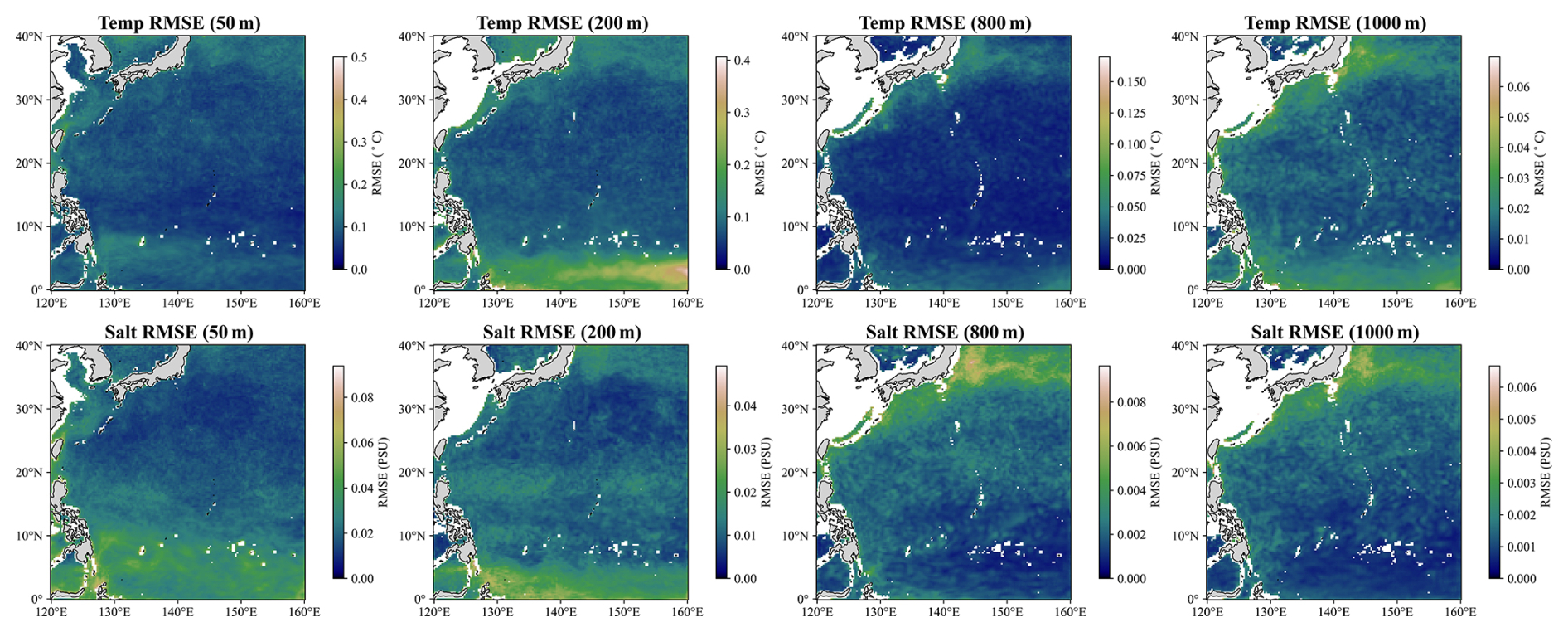
Figure 11 Spatial distribution of the RMSE between the reconstructed data and the GLORYS2V4 data at depths of 50, 200, 800, and 1000 m in 2023.

These results suggest that the proposed neural network can infer subsurface thermal structures from surface observational data alone to a considerable extent. The relatively high spatial consistency and low reconstruction errors across all depths indicate good generalization performance. The stronger performance in the intermediate and deep layers further suggests that the model is able to capture relatively stable, large-scale oceanic states.

3.3.2 Comparison of the Model Reconstructions with WOD T–S Profiles

To objectively evaluate the reliability of the reconstructed products, WOD T–S profiles data were introduced for error analysis. After quality control, a total of 7833 T–S profiles were selected within the study region for the year 2023, as shown in Fig. 12a.

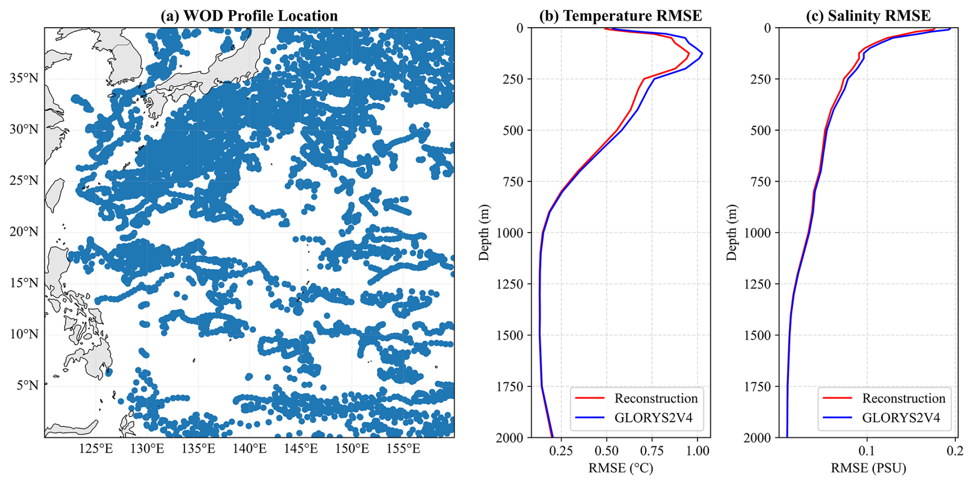
Figure 12 (a) Spatial distribution of WOD observational profiles in 2023; (b) variation of temperature RMSE with depth between the reconstructed temperature data and the WOD temperature profiles; (c) variation of salinity RMSE with depth between the reconstructed salinity data and the WOD salinity profiles.

At the geographical coordinates corresponding to each T–S profile, reconstructed temperature and salinity data as well as GLORYS2V4 temperature and salinity data were extracted to compute the RMSE. The vertical RMSE distributions between the WOD T–S profiles and the reconstructed and GLORYS2V4 T–S data are shown in Fig. 12b–c.

In 2023, the T–S profile distribution within the study region was relatively uniform (Fig. 12a). Overall, the reconstructed and GLORYS2V4 T–S data show similar vertical RMSE distributions (Fig. 12b and c). For temperature, both datasets show higher RMSE values in the subsurface layers (Fig. 12b), while for salinity, the RMSE values decrease gradually with depth (Fig. 12c). The reconstructed T–S data generally outperform GLORYS across all depths. The mean RMSE of the reconstructed temperature over the full depth range is 0.4907 °C, lower than that of GLORYS (0.5241 °C). Similarly, the mean RMSE of the reconstructed salinity (0.0699 PSU) is slightly lower than that of GLORYS (0.0747 PSU). Overall, the reconstructed T–S fields agree more closely with the in situ observations, suggesting improved reconstruction fidelity.

The spatial distribution of RMSE between the reconstructed data and the WOD profiles is shown in Fig. 13. In both datasets, larger errors are found along the western boundary currents and near-coastal regions, while smaller errors appear in the interior of the basin (Fig. 13a–b and d–e). The difference maps indicate that the reconstructed temperature and salinity, especially temperature, generally perform better across the study region (Fig. 13c and f). Overall, the reconstructed T–S fields are more consistent with the WOD T–S profiles, indicating improved agreement with observations.

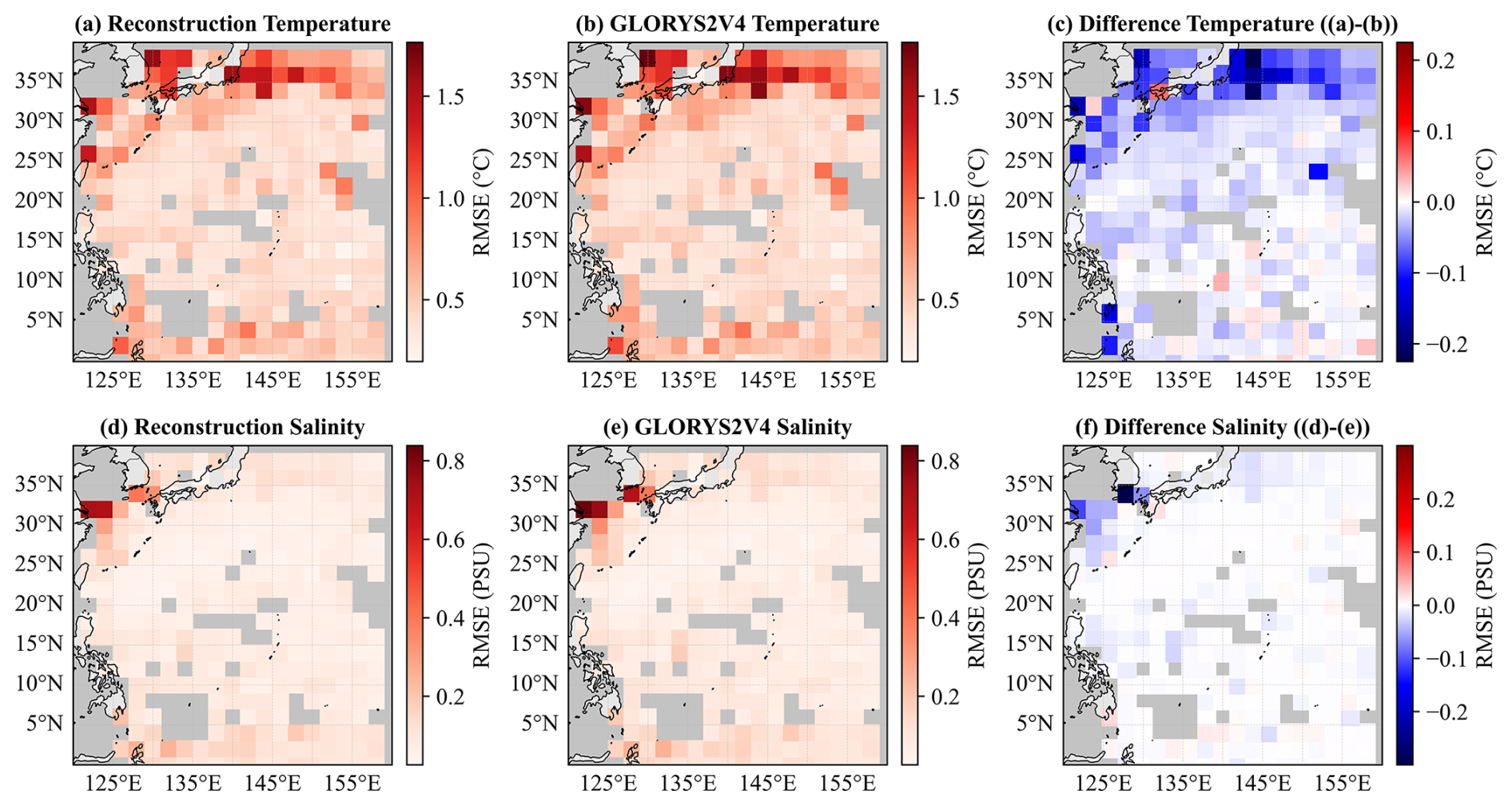
Figure 13 RMSE between reconstruction and WOD profiles (left), RMSE between GLORYS2V4 and WOD profiles (middle), and their difference (right). The first row shows the results for temperature data, and the second row shows the results for salinity data.

Since the 3D-U-Net$++$ model learns the mapping from surface variables (SST, SSH) to subsurface layers based on the statistical relationships embedded in GLORYS2V4, the reconstructed outputs inevitably inherit some characteristics of this reanalysis product. However, this does not necessarily mean that the model merely reproduces the reanalysis climatology. As shown in Figs. 12 and 13, the high consistency between the reconstruction and the independent WOD profiles suggests that the model generalizes the learned relationships to actual oceanic conditions rather than simply overfitting to the reanalysis statistics. This indicates that the method reconstructs independent oceanic variability driven by surface inputs while using the reanalysis data to constrain the vertical thermohaline structure. Therefore, the reconstructed product may be interpreted as combining real-time satellite-observed surface variability with the vertical structure learned from GLORYS2V4.

3.4 Long-term Statistical Analysis

To further verify the robustness and reliability of the proposed reconstruction method in generating T–S data, a long-term statistical analysis of the reconstructed results was conducted. Specifically, after the neural network training was completed, SST and SSH data from 1993 to 2023 were used as inputs to reconstruct the corresponding T–S fields for the same period. The reconstructed results were then compared with all available WOD T–S profile observations from 1993 to 2023 to perform an error analysis. For the long-term comparison, six reference datasets – GLORYS2V4, HYCOM, ORAS5, HGEM, IPRC Argo, and CGOF – were employed.

During the period from 1993 to 2023, a total of 353 154 WOD T–S profiles were collected within the study region. For clarity of presentation, the RMSE values calculated from these samples were averaged on a monthly basis. The RMSE results for temperature and salinity are presented in Figs. 14 and 15, respectively. Since the valid time span of the IPRC Argo dataset is 2005–2020, the results were divided into three distinct periods to better demonstrate the effectiveness of the transfer learning strategy: 1993–2004 (Figs. 14a and 15a), 2005–2019 (Figs. 14b and 15b), and 2020–2023 (Figs. 14c and 15c). The variation of RMSE with depth was also calculated based on the WOD samples, and the results are shown in Fig. 15.

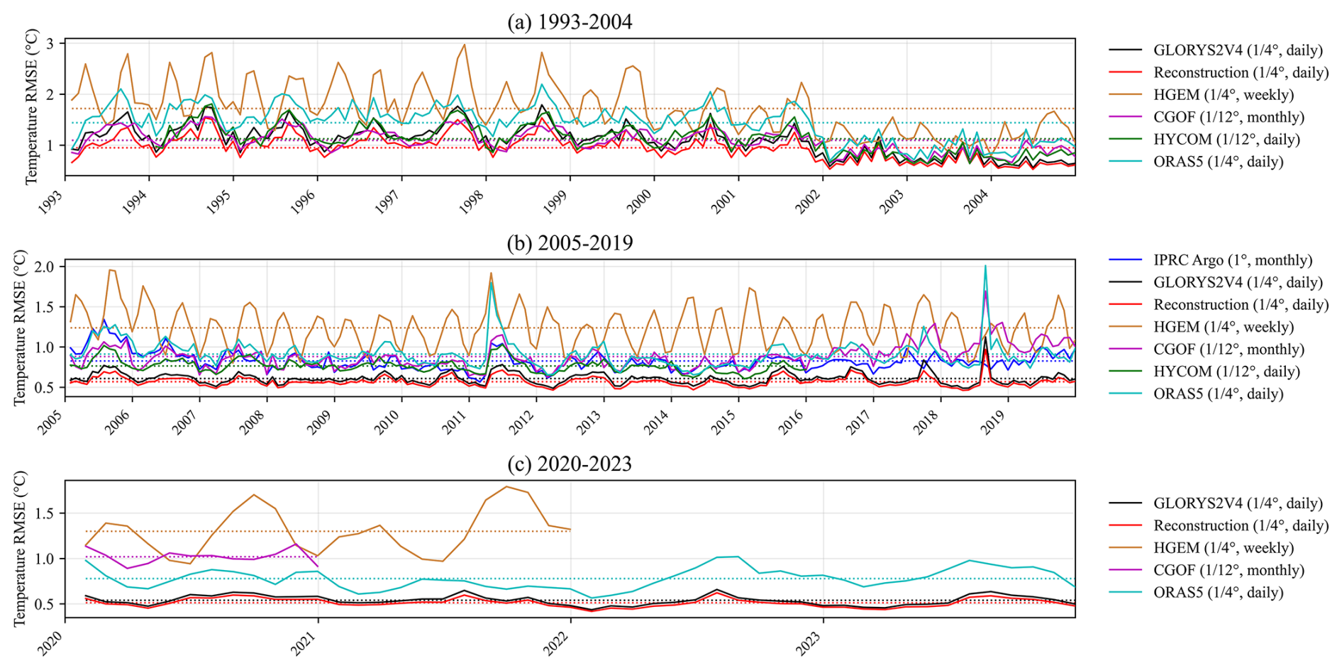
Figure 14 Monthly time series of RMSE of various temperature datasets compared with WOD temperature profiles in the upper 2000 m: (a) 1993–2004, (b) 2005–2019, and (c) 2020–2023.

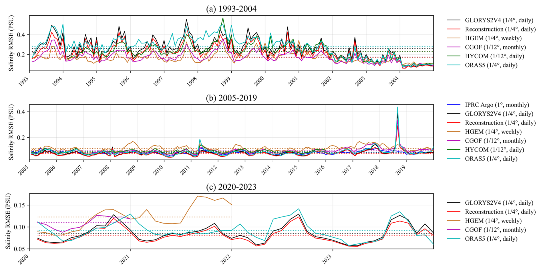
Figure 15 Monthly time series of RMSE of various salinity datasets compared with WOD temperature profiles in the upper 2000 m: (a) 1993–2004, (b) 2005–2019, and (c) 2020–2023.

As shown in Fig. 14, throughout the entire study period (1993–2023), the reconstructed temperature field remains generally consistent with GLORYS2V4. Compared with the other reference datasets, the reconstructed temperature results are closer to the WOD observed temperature profiles (average RMSE: 0.677267 °C), suggesting higher accuracy and reliability.

Regarding salinity RMSE, during 1993–2004, HGEM shows the smallest errors (0.1681 PSU) among the compared datasets (Fig. 15a); however, in the subsequent periods, the reconstructed salinity data align more closely with the WOD salinity profiles, indicating better stability and adaptability of the proposed method for salinity reconstruction. Over the full period (1993–2023), the reconstructed salinity shows the closest agreement with the WOD observed salinity, with an RMSE of 0.1282 PSU.

The RMSE values of all datasets are relatively high during 1993–2004. This is mainly because the number of WOD T–S profiles during this period was limited, and most observations were concentrated along the Japanese coast. This region lies within the highly dynamic Kuroshio Current zone, where the vertical thermohaline structure exhibits strong cross-front differences and prominent mesoscale to submesoscale variability, leading to larger assimilation errors between model outputs and observations.

Notably, in the proposed transfer learning strategy, the pretraining data were derived from the 2005–2019 IPRC Argo T–S dataset. Nevertheless, the reconstruction results show greater reliability than GLORYS2V4 over the full 1993–2023 period. This suggests that the model is not strictly limited by the temporal range of the training data and has good generalization capability.

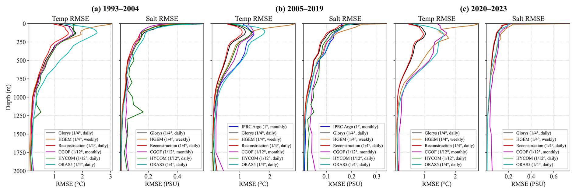
Figure 16 RMSE profiles of different temperature and salinity datasets compared with WOD T–S profiles during (a) 1993–2004, (b) 2005–2019, and (c) 2020–2023.

The variation of RMSE with depth shown in Fig. 16 indicates that, throughout the evaluation period, the reconstructed temperature consistently exhibits the lowest RMSE at all depth levels compared with the other temperature datasets. For salinity, during 1993–2004, the CGOF salinity data show a slight advantage at depths shallower than 130 m; however, below 130 m, the reconstructed salinity data remain more consistent with the WOD salinity profiles (Fig. 16a). During 2005–2019, the IPRC Argo salinity dataset achieves the lowest RMSE near the surface (50 m), while at all other depths, the reconstructed salinity data match the in situ observations more closely (Fig. 16b). Overall, the reconstructed T–S fields exhibit good reliability and stability across all depth layers, further supporting the robustness and accuracy of the proposed reconstruction approach.

To more intuitively illustrate the relationships between various T–S datasets and the WOD T–S profiles, four representative depths (50, 200, 800, and 1000 m) were selected. At each depth, density scatter plots were drawn for the reconstructed T–S data, as well as for the GLORYS2V4, HGEM, IPRC Argo, and CGOF datasets, in comparison with the WOD in situ observations. The density scatter plots of temperature and salinity data are shown in Figs. 17 and 18, respectively.

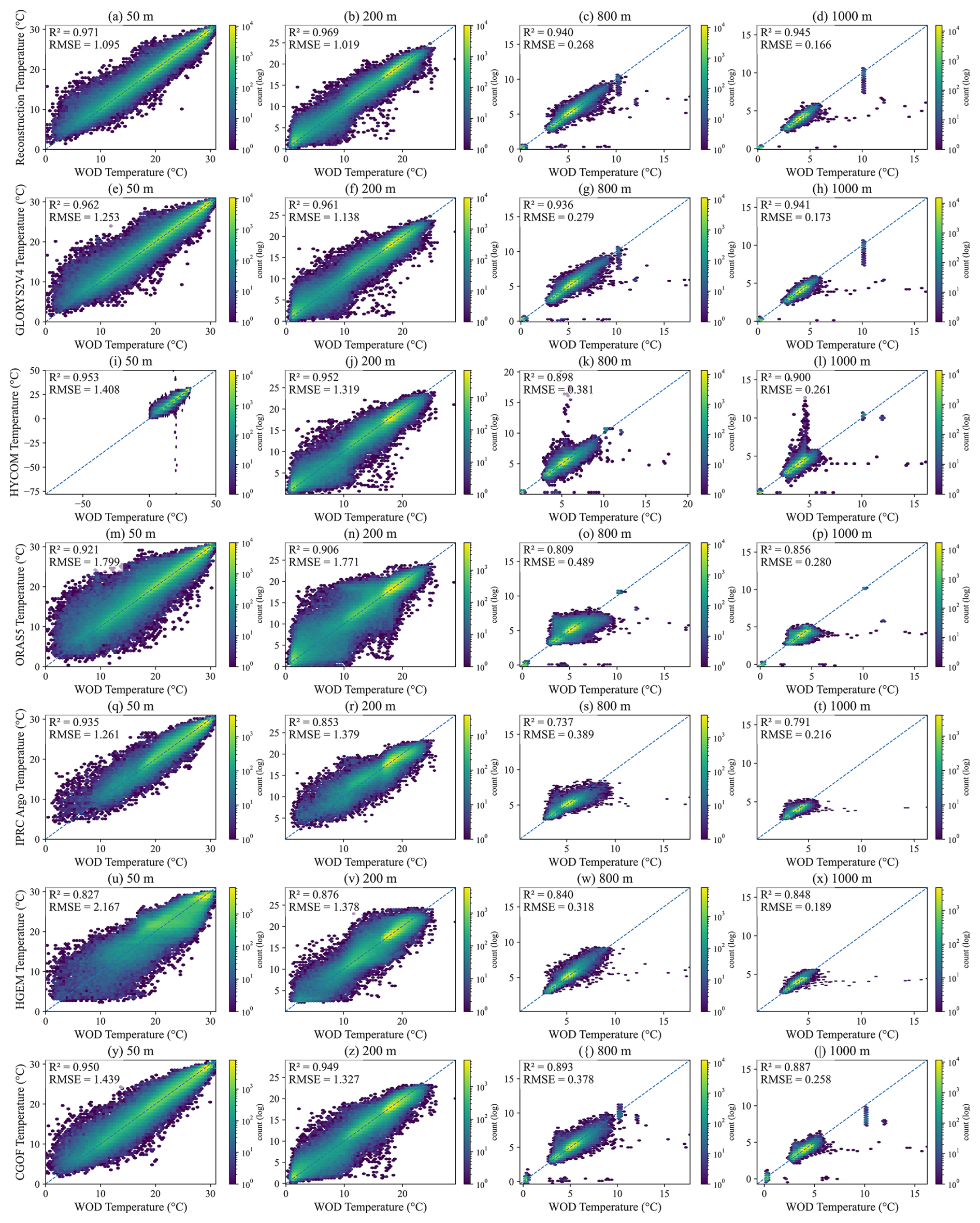
Figure 17 Density scatter plots between different temperature datasets and WOD observed temperature profiles at four representative depths (50, 200, 800, and 1000 m) over the period of 1993–2023.

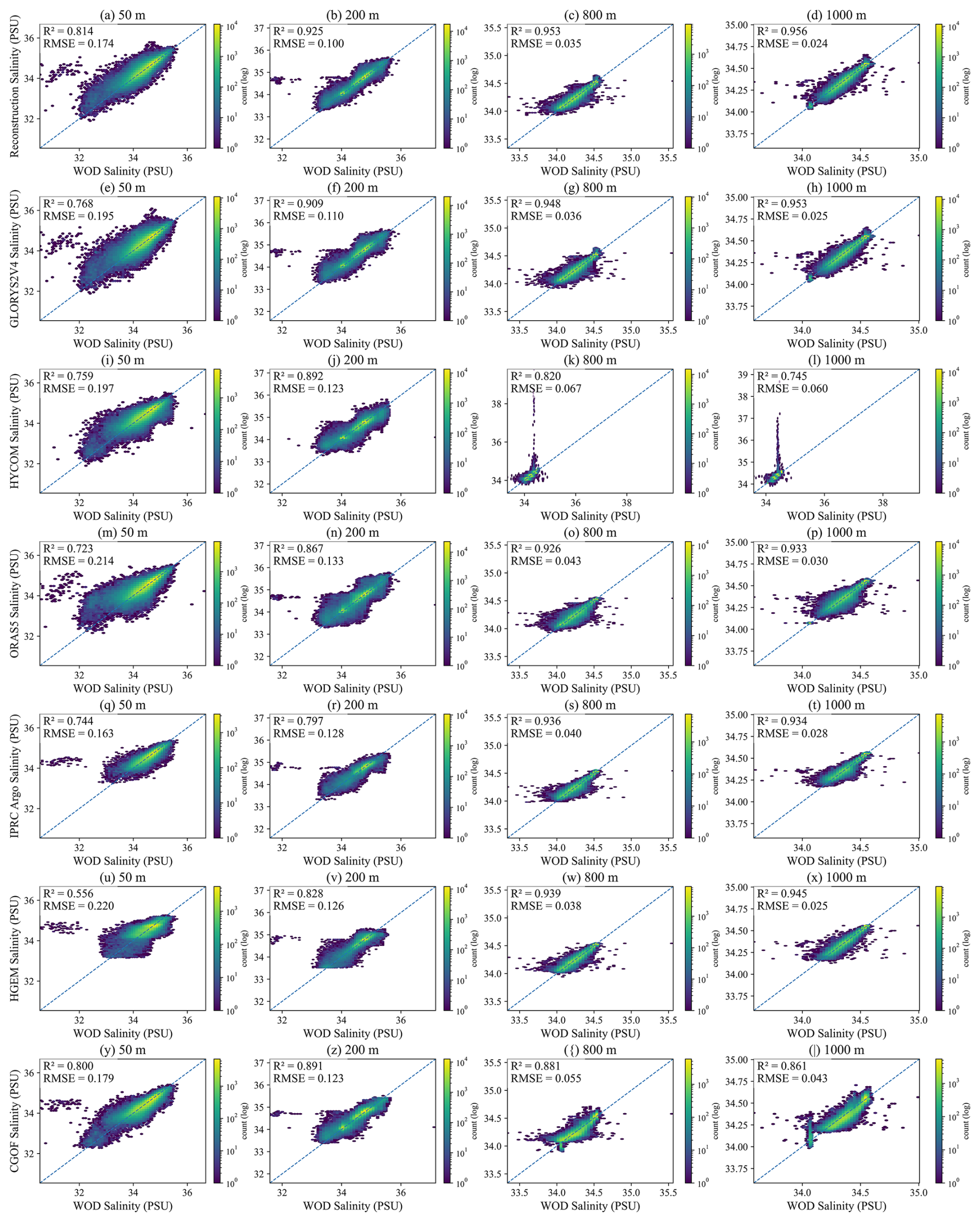
Figure 18 Density scatter plots between different salinity datasets and WOD observed salinity profiles at four representative depths (50, 200, 800, and 1000 m) over the period of 1993–2023.

From Figs. 17 and 18, the correlation and bias characteristics between each dataset and the WOD in situ observations at different depths can be clearly seen. The reconstructed results proposed in this study show the highest consistency and the most compact distributions at all four representative depths. The scatter clouds are densely concentrated along the 1:1 diagonal line, with distinct density peaks and narrow bias distributions, indicating that the model can reproduce the large-scale oceanic thermohaline structure reasonably well.

At the surface layer (50 m), all datasets show a certain degree of dispersion, influenced by air–sea exchanges and seasonal mixing. However, the reconstructed results show the smallest dispersion range, with little apparent systematic overestimation or underestimation. In contrast, GLORYS2V4 and CGOF exhibit slight offsets in regions of high temperature and salinity, reflecting weaker performance in strongly variable areas. At 200 m depth, the relationship between the reconstructed results and the WOD observations becomes more linear, suggesting that the model captures the thermohaline gradient structure near the upper boundary of the thermocline reasonably well. The HGEM and Argo products show slightly more scattered distributions at this depth, indicating moderate biases in reproducing the upper-to-mid-layer thermohaline structure. In the intermediate and deep layers (800 and 1000 m), the reconstructed results maintain good agreement with the observations, with highly concentrated scatter and very low RMSE values. This suggests that the model performs well not only at the surface but also in reconstructing deep thermohaline structures. In comparison, GLORYS2V4 and CGOF exhibit slightly broader scatter distributions and a tendency toward underestimation, while HGEM shows increased dispersion, reflecting weaker deep-layer constraints.

Overall, the density scatter distributions for both temperature and salinity indicate that the reconstructed data achieve the highest correlation and lowest errors relative to the WOD observations, suggesting consistent performance across the evaluated depth range. These results support the high accuracy and robustness of the proposed reconstruction method under multi-scale and multi-depth conditions. Furthermore, they indicate that the developed neural network effectively integrates multi-source information during the long-term reconstruction process, capturing rapid upper-ocean variability while also improving the reconstruction of deep-layer equilibrium structures, thereby providing a solid foundation for high-quality three-dimensional thermohaline reanalysis.

4 Data availability

The data used in this study are available for consultation as described in Sect. 2.1. The T–S data reconstructed using the method proposed in this study are freely accessible at https://doi.org/10.57760/sciencedb.31950 (Wang et al., 2025).

5 Discussion and Conclusion

To achieve real-time and accurate reconstruction of daily three-dimensional T–S fields ($\mathrm{1}/\mathrm{4}$°, 26 layers, 5–2000 m) in the northwestern Pacific (0–40° N, 120–160° E), this study proposes an attention-enhanced 3D U-Net$++$ reconstruction framework that relies solely on real-time available SST and SSH data. The attention enhanced 3D U-Net$++$ architecture provides a mechanism for cross-scale feature aggregation and selective information gating through deep skip connections. The attention gates highlight temporal surface features that are more strongly correlated with the target depth layers along the multi-resolution pathways, thereby mitigating noise propagation and over-smoothing. Combined with the 3D encoder–decoder structure, this design enhances the preservation of vertical gradients and frontal structures in the reconstructed fields. The network takes 26 consecutive days of SST and SSH as input, which effectively alleviates the intrinsic challenge of mapping from limited surface inputs to full-depth outputs. A single-time surface-to-volume mapping is inherently underdetermined, resembling a super-resolution problem. By incorporating inter-day evolution, the model can extract implicit constraints associated with subseasonal variability, circulation, and mixing processes from the temporal continuity of surface signals, thereby reducing non-uniqueness and improving the discriminability of vertical structures. In addition, a transfer learning strategy is employed. The model is first pretrained using monthly SST/SSH and IPRC-Argo datasets to learn observation-dominated low-frequency spatiotemporal signals and stable structures. It is then retrained using daily SST/SSH and GLORYS2V4 data to capture the dynamic processes and assimilation mechanisms embedded in the reanalysis fields.

Analysis results demonstrate that, both on the validation set and in long-term statistical evaluations, the reconstructed T–S fields are more consistent with in situ observation profiles, verifying the reliability and accuracy of the proposed method for subsurface ocean data inversion. Despite the promising results, several limitations and uncertainties must be acknowledged. First, the reconstructed fields are inevitably influenced by the GLORYS2V4 reanalysis used as the fine-tuning target. As a result, the final outputs inherit part of the statistical and dynamical structure embedded in this reanalysis product, together with its associated uncertainties. Second, the validation data from WOD are unevenly distributed in space and time, which means that the reported validation statistics mainly reflect the model performance in regions and periods with available in situ profiles. Finally, the uncertainty of the reconstructed fields is likely to vary with depth and region.

The data obtained in this study provide crucial support for revealing mesoscale ocean dynamic processes. Furthermore, they lay a solid foundation for quantitatively estimating key elements, including ocean mass transport, heat, and salinity fluxes. In the future, these data will be valuable for advancing the study of mesoscale ocean dynamics. They also show great potential for improving ocean model simulations and enhancing climate prediction accuracy.