Reconstructing two-decade daily high-resolution seamless global land XCO₂ records using a hybrid Transformer–BiLSTM model

Accurate and temporally continuous global observations of atmospheric carbon dioxide (XCO₂) are essential for climate monitoring and emission assessment. However, satellite-based XCO₂ observations are often spatially incomplete and temporally discontinuous, while existing products typically suffer from coarse spatial resolution, hindering the detection of fine-scale emission changes. Here, we developed a novel spatiotemporal Transformer–BiLSTM deep-learning network that combines the Transformer's ability to model long-range spatial dependencies through self-attention mechanisms with the BiLSTM's ability to capture temporal dynamics. The network assimilates multisource data from satellite observations, meteorological reanalysis, and precursor gases to reconstruct a global, daily, and seamless XCO₂ dataset over land at 0.1° spatial resolution from 2003 to 2022. Independent validation of the data-fused XCO₂ product against Total Carbon Column Observing Network (TCCON) measurements shows excellent agreement, with an R² of 0.99, an RMSE of 1.10 ppm, and a mean bias of 0.01 ppm. After bias correction, cross-satellite consistency is further enhanced, achieving a sample-based CV-R² of 0.99 and an RMSE of 0.36 ppm. The dataset provides accurate daily XCO₂ estimates over global land surfaces, enabling investigations of spatial heterogeneity and regional-to-local XCO₂ enhancement patterns linked to anthropogenic emissions and biomass-burning events. The record reveals a persistent global increase in atmospheric XCO₂ over the past two decades, with a mean growth rate of 2.24 ppm yr⁻¹ (p<0.001). It reliably resolves global XCO₂ variability across a wide range of temporal scales, from day-to-day fluctuations to long-term trends. It consistently captures large-scale climate-driven signals, such as ENSO-related interannual variability, and short-lived XCO₂ enhancements associated with major wildfire events, demonstrating its capability to represent both persistent and episodic emission signals. This high-resolution, daily global XCO₂ (GlobalHighXCO₂) product provides a valuable resource for carbon-cycle research, atmospheric model evaluation, and emission monitoring, and is publicly available at https://doi.org/10.5281/zenodo.18220962 (Qu and Wei, 2026).

1 Introduction

Carbon dioxide (CO₂) is a principal greenhouse gas that plays a significant role in driving global climate change (Romanov, 2017). Driven by anthropogenic activities and extreme wildfires, the global mean atmospheric CO₂ concentration reached 419.31±0.15 ppm (parts per million) in 2023, approximately 50 % higher than preindustrial levels, making it a major contributor to ongoing climate change (Friedlingstein et al., 2023). In response to rising CO₂ levels, the international community adopted the Paris Agreement in 2015, aiming to limit global warming to well below 2 °C compared to preindustrial levels. Owing to its long atmospheric lifetime, CO₂ accumulates and exerts sustained radiative forcing, resulting in long-term climate impacts (Lee et al., 2023; Kemp et al., 2022). Accurate long-term monitoring of atmospheric CO₂ is therefore essential for advancing understanding of the global carbon cycle, verifying national emission-reduction commitments, and informing effective climate-mitigation policies.

Atmospheric column-averaged dry-air mole fractions of CO₂ (XCO₂) are commonly quantified using ground-based networks and satellite remote sensing (Petzold et al., 2015; Huang et al., 2024a). Ground-based networks, such as the Total Carbon Column Observing Network (TCCON), provide accurate and stable point-based measurements; however, their sparse spatial distribution limits their ability to support refined assessments of the global carbon budget and regional carbon fluxes (Li et al., 2024a). Satellite remote sensing offers a complementary approach by providing broad spatial coverage for regional and global-scale XCO₂ monitoring, but it generally has a lower temporal sampling frequency (Buchwitz et al., 2015). Since the early 2000s, a series of satellite missions has progressively advanced XCO₂ observations in accuracy, spatial resolution, and temporal coverage. The SCanning Imaging Absorption spectroMeter for Atmospheric CHartographY (SCIAMACHY) aboard the Environmental Satellite (Envisat), launched in 2002, was the first satellite instrument to provide global XCO₂ observations until 2012 (Bovensmann et al., 1999). Subsequently, a new generation of spaceborne sensors, including Japan's Greenhouse Gas Observing Satellite (GOSAT) (Kuze et al., 2009; Butz et al., 2011) NASA's Orbiting Carbon Observatory-2/3 (OCO-2/3) (Crisp et al., 2017), and China's TanSat (Yang et al., 2018), have substantially advanced top-down constraints on carbon sources and sinks. These satellite data have become indispensable for understanding large-scale carbon cycle processes. Despite major advances in satellite XCO₂ observations, existing products remain limited by cloud and aerosol contamination, surface effects, and orbital sampling constraints (He et al., 2022). These gaps severely restrict the accurate analysis of seasonal and interannual changes in regional carbon fluxes and impede the detection of carbon-cycle anomalies associated with extreme climate events (Ma et al., 2021; Li et al., 2022).

To address spatial gaps in satellite XCO₂ observations, researchers have explored a range of data fusion and reconstruction methods. Early studies primarily relied on geospatial interpolation techniques, such as kriging and its spatiotemporal extensions (Hammerling et al., 2012; He et al., 2020; Wang et al., 2025; Chen et al., 2024). While effective in data-rich regions, these methods often assume stationary spatial correlations, leading to large uncertainties in sparsely observed areas. Global reanalysis products, including CAMS and CarbonTracker, provide spatially complete fields but typically have coarse spatial resolution, limiting their ability to resolve regional emission sources (Hua et al., 2024). Traditional machine-learning (ML) models, such as Random Forest and XGBoost, have been widely adopted for XCO₂ reconstruction due to their strong nonlinear fitting capabilities (Ma et al., 2021; Zhang et al., 2023; Liang et al., 2023). However, these approaches generally treat reconstruction as a point-wise regression problem, neglecting the intrinsic spatiotemporal autocorrelation and physical coherence of atmospheric fields, which often results in spatially and temporally discontinuous outputs (Siabi et al., 2019; He et al., 2023b). Although some recent studies have attempted to incorporate spatiotemporal information (Wang et al., 2020; Liu et al., 2024), their ability to capture long-range temporal dependencies and cross-regional teleconnections remains limited (He et al., 2023a). The rapid development of deep learning (DL) has created new opportunities for reconstructing atmospheric data, overcoming the limitations of conventional linear models (Wei et al., 2024). Spatiotemporally aware DL architectures, particularly those integrating convolutional neural networks (CNNs) with recurrent neural networks such as long short-term memory (LSTM), have demonstrated strong capabilities in capturing fine-scale spatial patterns and temporal dependencies (He et al., 2024; Zhang and Liu, 2023; Wu et al., 2024). Recent studies have leveraged these models to fuse multisource satellite data (Huang et al., 2024a), incorporate temporal sequence features for daily XCO₂ estimation (Tian et al., 2024), and generate high-resolution regional products using deep autoencoders (Antezana Lopez et al., 2025; Li et al., 2025; Wang, 2026).

Despite these methodological advances, generating a truly seamless global daily XCO₂ dataset remains challenging. Harmonizing long-term records from multiple satellite missions, including SCIAMACHY, GOSAT, and OCO-2, introduces inter-sensor inconsistencies due to differences in instrument design and retrieval algorithms (Li et al., 2022; Chen et al., 2024). Although TCCON observations have been used for post hoc harmonization in some studies (Li et al., 2024b), bias correction is not yet fully integrated into the reconstruction framework. Moreover, existing global products often face a trade-off between spatial resolution and temporal frequency, providing either coarse daily fields or high-resolution monthly averages, thereby limiting their ability to capture short-term variability associated with extreme events such as wildfires (Liu et al., 2022; Rodrigues et al., 2025) and climate anomalies during El Niño episodes (Chatterjee et al., 2017; Betts et al., 2016). Consequently, a unified methodology that simultaneously addresses inter-satellite biases and captures long-range spatiotemporal dependencies at the global daily scale remains lacking.

To address these limitations, we develop a hybrid spatiotemporal deep-learning framework based on a Transformer–BiLSTM architecture for global daily XCO₂ reconstruction. Through jointly learning temporal evolution and spatial coherence from multisource satellite observations, reanalysis data, and auxiliary predictors, the proposed approach effectively captures complex spatiotemporal variability in atmospheric XCO₂ fields. Leveraging this framework, we generate a seamless global daily XCO₂ dataset over land at 0.1° resolution spanning 2003–2022. A TCCON-based bias-correction strategy is incorporated to harmonize multiple satellite mission records and ensure long-term temporal consistency. In addition, explainable artificial intelligence techniques are employed to enhance model interpretability and quantify the relative contributions of key drivers of XCO₂ variability. Together, these advances provide a consistent long-term XCO₂ product suitable for carbon-cycle analysis, emission monitoring, and climate-related applications.

2 Materials and methods

2.1 Multisource data

2.1.1 Satellite, reanalysis, and ground-based XCO₂ data

Satellite-based XCO₂ retrievals from SCIAMACHY, GOSAT, and OCO-2 were used as the primary observational constraints in this study. SCIAMACHY, onboard Envisat and operating from 2002 to 2012, provided global XCO₂ observations at a resolution of 30×60 km² approximately every 30 d, retrieved using the Bremen Optimal Estimation DOAS (BESD) algorithm (Bovensmann et al., 1999; Buchwitz et al., 2005; Reuter et al., 2011). GOSAT, launched in 2009, provides near-global coverage at 10.5 km spatial resolution every 3 d through its Fourier Transform Spectrometer. OCO-2, operating since 2014, provides XCO₂ measurements at 1.29×2.25 km² resolution every ∼16 d using three grating spectrometers (Crisp, 2015). Here, we used the SCIAMACHY BESD products from 2003 to 2009, GOSAT Level 2 XCO₂ Version 9r products from 2010 to 2014, and OCO-2 Level 2 XCO₂ Lite Version 11r product from 2015 to 2022. All retrievals underwent standard quality control, and only high-quality observations were retained. In addition, the Copernicus Atmosphere Monitoring Service (CAMS) provides a global atmospheric composition reanalysis, offering continuous greenhouse gas fields from 2003 to the present at 0.75°×0.75° horizontal resolution and a 3 h temporal resolution (Agustí-Panareda et al., 2023). CAMS provides spatially complete and consistent estimates of large-scale XCO₂ patterns and was also employed in this study.

Ground-based observations were obtained from the TCCON, which provides high-precision XCO₂ measurements with an average uncertainty of approximately 0.2 %. The network offers sub-daily temporal sampling, typically including multiple observations per clear-sky day, and serves as a standard reference for the validation of satellite XCO₂ retrievals (Wunch et al., 2017). We used all available 31 stations in the GGG2020 release, distributed across global land areas (Fig. 1), serving as the reference for assessing reconstruction performance and guiding bias correction. To independently evaluate the bias-corrected daily XCO₂ dataset, we used surface flask measurements from the Observations Package (ObsPack) dataset, including 41 land-based sites (Fig. 1). Only stations with a quality inspection flag of 1 or 2 were retained to ensure consistency with the World Meteorological Organization X2019 calibration scale.

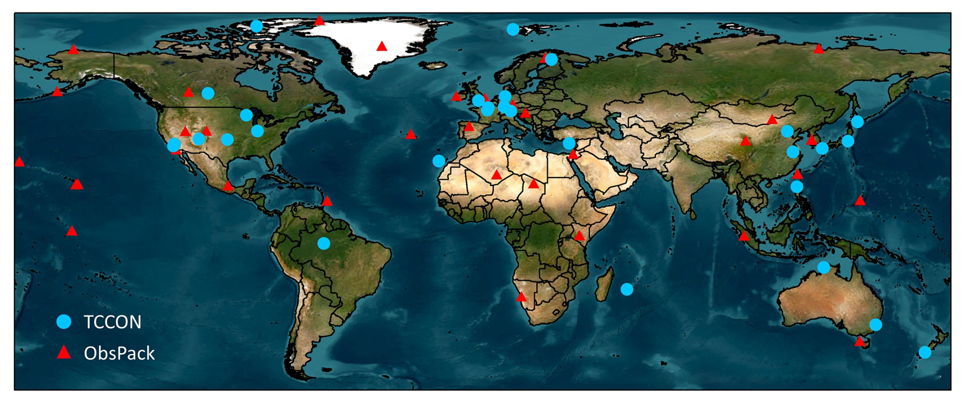
Figure 1 Geographic locations of TCCON (Total Carbon Column Observing Network; blue dots) and ObsPack (Observations Package; red triangles) observation stations.

2.1.2 Meteorological and auxiliary variables

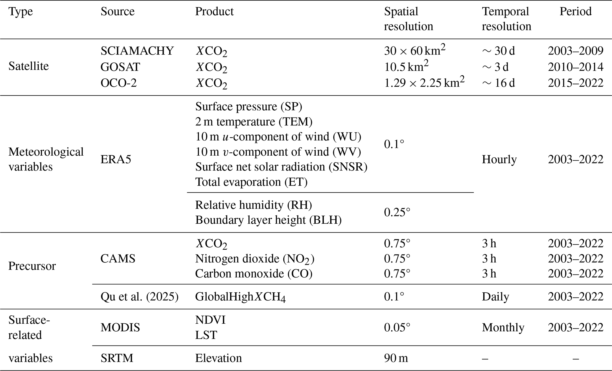
Meteorological variables relevant to atmospheric CO₂ variability were obtained from the ERA5-Land hourly reanalysis at a spatial resolution of 0.1°×0.1°, including surface pressure (SP), 2 m air temperature (TEM), surface net solar radiation (SNSR), total evaporation (ET), and 10 m u- and v-components of wind (WU and WV). Boundary layer height (BLH) and relative humidity (RH) were obtained from the ERA5 reanalysis at 0.25°×0.25° resolution. To capture short-lived atmospheric precursors associated with anthropogenic and biomass-burning emissions, we included daily nitrogen dioxide (NO₂) and carbon monoxide (CO) total columns from the CAMS analysis, as well as column-averaged methane (XCH₄) derived from our previous study (Qu et al., 2025), which were used as proxies for fossil-fuel combustion and fire-related emissions (Reuter et al., 2019). Land-surface conditions were characterized using MODIS products, including monthly normalized difference vegetation index (NDVI) and land surface temperature (LST), which are closely related to terrestrial carbon uptake and surface–atmosphere carbon exchange (Huang et al., 2015; Li et al., 2025). Topographic effects were represented using the Shuttle Radar Topography Mission (SRTM) digital elevation model (DEM) at 90 m resolution. Table 1 provides an overview of all data sources used in this study.

Table 1 Summary of the datasets used for XCO₂ reconstruction in this study.

2.2 Model development and construction

2.2.1 Transformer–BiLSTM framework

In this study, we proposed a hybrid spatiotemporal Transformer–BiLSTM deep-learning framework to capture both spatial and temporal dependencies. The input predictors are first processed by a Transformer encoder (Vaswani et al., 2017), which models long-range spatial dependencies at regional and global scales through multi-head self-attention and position-wise feed-forward layers, without relying on local receptive fields. Each location's feature vector is projected into query (Q), key (K), and value (V) vectors, and the resulting attention scores quantify the influence of all other locations on that location. The multi-head attention mechanism integrates complementary spatial relationships across multiple feature subspaces, enabling the model to explicitly capture planetary-scale influences, such as atmospheric teleconnections and large-scale weather systems, on regional XCO₂ concentrations.

The spatially encoded features generated by the Transformer are subsequently passed to a Bidirectional Long Short-Term Memory (BiLSTM) network, which learns forward and backward temporal dependencies by integrating both past and future information (Zhang et al., 2020). This sequence-to-sequence formulation effectively captures temporal variability arising from diurnal cycles, synoptic weather variations, and seasonal biospheric processes affecting XCO₂ concentrations, thereby generating comprehensive spatiotemporal feature representations for each grid cell.

The resulting spatiotemporal features are finally passed through a multilayer perceptron (MLP) block, followed by a fully connected linear layer that projects the fused features to scalar daily XCO₂ estimates for each grid cell. To effectively capture the complex spatiotemporal dynamics of atmospheric XCO₂, we designed a weighted spatiotemporal loss function that accounts for intrinsic temporal continuity and spatial correlation, in contrast to the standard mean squared error (MSE) loss function:

$$\begin{array}{}\text{(1)}& \begin{array}{rl}{L}_{X{\mathrm{CO}}_{\mathrm{2}}}& ={\displaystyle \frac{\mathrm{1}}{N}}\sum _{i=\mathrm{1}}^N{\left(y_i-{\widehat{y}}_i\right)}^{\mathrm{2}}+{\mathit{\chi }}_{\mathrm{1}}{\displaystyle \frac{\mathrm{1}}{N-\mathrm{1}}}\sum _{i=\mathrm{2}}^N{\left(\mathrm{\Delta }{y}_i-\mathrm{\Delta }{\widehat{y}}_i\right)}^{\mathrm{2}}\\ & +{\mathit{\chi }}_{\mathrm{2}}{L}_{\mathrm{spatial}}\end{array}\end{array}$$

where y_i and ${\widehat{y}}_i$ denote the observed and predicted XCO₂ values for the ith sample, respectively, and Δy_i and $\mathrm{\Delta }{\widehat{y}}_i$ represent the corresponding temporal differences between consecutive time steps. The first term enforces point-wise reconstruction accuracy, the second term promotes temporal consistency, and L_spatial introduces a Laplacian-based spatial smoothness constraint to preserve coherence among neighboring 0.1° grid cells. The hyperparameters χ₁=0.5 and χ₂=0.01, which regulate the temporal and spatial regularization terms, respectively, were determined via a grid search.

During model construction, the dataset was randomly partitioned into training, validation, and testing sets at a ratio of $\mathrm{8}:\mathrm{1}:\mathrm{1}$. The temporal encoder was implemented as a single-layer bidirectional LSTM (BiLSTM) with 64 hidden units per direction, yielding a 128-dimensional output feature. A dropout rate of 0.5 was applied to mitigate overfitting. The Transformer module comprised 4 encoder layers, each with 64-dimensional hidden layers and 4 attention heads, with ReLU activation functions applied between layers to enhance learning and facilitate sparse feature extraction. The Transformer–BiLSTM model was trained with the Adam optimizer, an initial learning rate of 0.001, and a batch size of 256. To optimize convergence, a learning-rate scheduler reduced the learning rate by a factor of 0.1 every 10 epochs if the validation loss did not improve. Training continued for up to 200 epochs, with early stopping applied if the validation loss failed to decrease for 15 consecutive epochs (Yeom et al., 2021).

2.2.2 Two-phase reconstruction workflow

To address the spatial discontinuity of raw satellite observations and the limited coverage of TCCON ground-based stations, we designed a sequential two-phase “fusion-then-correction” reconstruction workflow that decouples spatial pattern learning from magnitude calibration (Fig. 2).

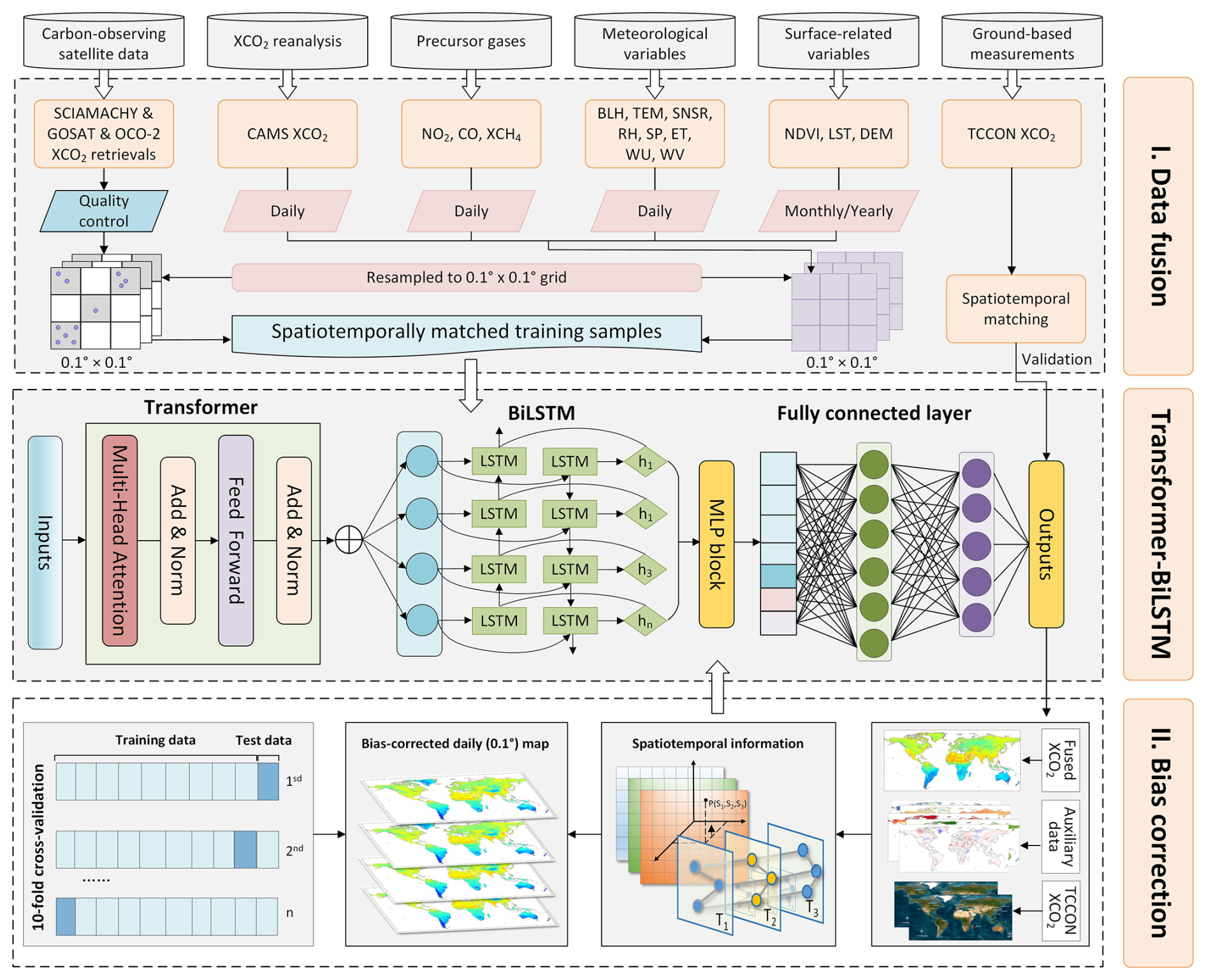
Figure 2 Workflow for generating a global, daily, seamless XCO₂ dataset at a spatial resolution of 0.1°×0.1° using the developed Transformer–BiLSTM framework.

Phase 1: data fusion

The objective of this stage is to reconstruct a spatially continuous global XCO₂ field from sparse and discontinuous satellite observations. The Transformer–BiLSTM model uses XCO₂ retrievals from SCIAMACHY, GOSAT, and OCO-2 as training targets and integrates multisource predictors, including atmospheric variables (XCH₄ from our previous study, Qu et al., 2025, as well as CAMS XCO₂, NO₂, and CO columns), ERA5 meteorology variables (BLH, TEM, SNSR, RH, SP, ET, WU, and WV), and land-surface variables (NDVI, LST, and DEM). In addition, spatiotemporal encoding vectors are incorporated to characterize geographic and temporal dependencies. Specifically, spatial coordinates are represented using three Euclidean spherical functions (P_S = S1, S2, S3), while temporal information is encoded using three helix-shaped trigonometric functions (P_T = T1, T2, T3), enabling the model to capture spatial heterogeneity and temporal variability (Wei et al., 2023; Qu et al., 2025). The output of this stage is a preliminary global XCO₂ dataset at 0.1°×0.1° spatial resolution, providing a seamless and spatially continuous field for the subsequent bias-correction stage.

$$\begin{array}{}\text{(2)}& \begin{array}{rl}X{{\mathrm{CO}}_{\mathrm{2}}}^{\mathrm{Satellites}}\sim & f_{\mathrm{Transformer}\text{-}\mathrm{BiLSTM}}\left(X{{\mathrm{CO}}_{\mathrm{2}}}^{\mathrm{CAMS}},\right.\\ & {{\mathrm{NO}}_{\mathrm{2}}}^{\mathrm{CAMS}},{\mathrm{CO}}^{\mathrm{CAMS}},X{\mathrm{CH}}_{\mathrm{4}},\\ & \left.\mathrm{Meteo},\mathrm{NDVI},\mathrm{LST},\mathrm{DEM},P_{\mathrm{S}},P_{\mathrm{T}}\right)\end{array}\end{array}$$

Phase 2: bias correction

Satellite XCO₂ retrievals often exhibit systematic biases arising from differences in sensor characteristics, retrieval algorithms, and temporal sampling. In this phase, the fused XCO₂ field from Phase 1 ($X{{\mathrm{CO}}_{\mathrm{2}}}^{\mathrm{Fusion}}$) is further calibrated through a bias-correction procedure using ground-based TCCON measurements as reference observations. The Transformer–BiLSTM model ingests the fused XCO₂ product together with the same auxiliary predictors used in the fusion stage, including atmospheric composition variables, meteorological variables, land-surface characteristics, and spatiotemporal encoding vectors. By learning the complex nonlinear relationships between satellite-dependent biases and environmental conditions, the model effectively reduces systematic errors while maintaining robust global generalization capability. The final output is a bias-corrected, seamless daily global XCO₂ dataset at 0.1°×0.1° spatial resolution with improved consistency across all satellite platforms:

$$\begin{array}{}\text{(3)}& \begin{array}{rl}X{{\mathrm{CO}}_{\mathrm{2}}}^{\mathrm{TCCON}}\sim & f_{\mathrm{Transformer}\text{-}\mathrm{BiLSTM}}\left(X{{\mathrm{CO}}_{\mathrm{2}}}^{\mathrm{Fusion}},\right.\\ & {{\mathrm{NO}}_{\mathrm{2}}}^{\mathrm{CAMS}},{\mathrm{CO}}^{\mathrm{CAMS}},X{\mathrm{CH}}_{\mathrm{4}},\\ & \left.\mathrm{Meteo},\mathrm{NDVI},\mathrm{LST},\mathrm{DEM},P_{\mathrm{S}},P_{\mathrm{T}}\right).\end{array}\end{array}$$

2.2.3 Innovations of the framework

The key innovation of our study lies in the synergistic integration of Transformer and BiLSTM modules to jointly model long-range spatial dependencies and temporal continuity. Specifically, the Transformer encoder utilizes self-attention mechanisms to capture non-local spatial relationships and global contextual information, which are critical for representing large-scale atmospheric transport and spatially heterogeneous carbon dynamics. In contrast, the BiLSTM module focuses on bidirectional temporal evolution, enabling the model to better characterize daily continuity, temporal autocorrelation, and persistent XCO₂ variability. Compared with conventional BiLSTM-attention frameworks (Wang et al., 2025), which mainly enhance sequential learning using local attention operations, our Transformer–BiLSTM architecture provides a substantially larger receptive field and stronger capability for jointly learning global spatiotemporal dependencies. In addition, we further introduce a weighted spatiotemporal loss function that jointly constrains reconstruction accuracy, temporal smoothness, and spatial coherence, thereby improving the temporal consistency and physical continuity of reconstructed daily XCO₂ fields. This differs from previous studies that mainly optimize point-wise reconstruction errors using standard loss functions such as MSE.

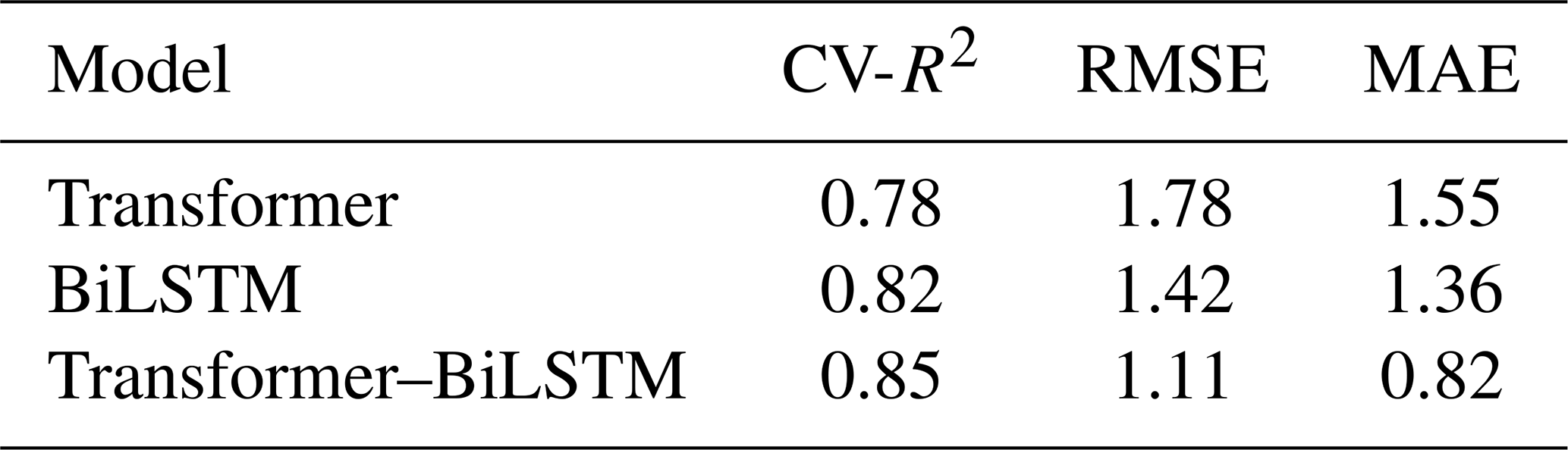
We further conducted an architecture-level ablation analysis comparing three backbone variants: BiLSTM, Transformer, and Transformer–BiLSTM (Table 2). The hybrid Transformer–BiLSTM model achieved the best overall performance, demonstrating the advantage of jointly modeling long-range spatial dependencies and temporal continuity.

Table 2 Ablation analysis of different backbone models for XCO₂ reconstruction.

Another important difference is that our framework is specifically designed for long-term multi-mission reconstruction. We propose a “data fusion + bias correction” workflow with explicit TCCON-guided bias correction to harmonize systematic discrepancies among SCIAMACHY, GOSAT, and OCO-2. Unlike previous studies that mainly focus on single-mission reconstruction performance, our framework explicitly addresses cross-mission inconsistencies and minimizes artificial temporal discontinuities caused by sensor replacement and orbital differences. Therefore, while previous studies have explored BiLSTM or attention-based approaches (Wang et al., 2025), the novelty of our study lies in the development of a Transformer–BiLSTM framework specifically designed for long-term, multi-mission daily XCO₂ reconstruction with improved temporal continuity and cross-mission consistency.

2.3 Validation method

The data-fused XCO₂ estimates were independently evaluated against TCCON XCO₂ measurements. For both the data-fused and bias-corrected XCO₂ products, a multi-strategy ten-fold cross-validation (10-CV) framework was applied using satellite and TCCON observations. Specifically, the sample-based CV randomly withheld 10 % of the daily grid-level samples to assess overall performance and internal consistency. The temporal-based CV withheld continuous blocks of daily data to evaluate the model's temporal generalization during periods without ground-based measurements. The spatial-based CV withheld spatially contiguous clusters of grid cells (1°×1°) to assess the model's capability to generalize to regions lacking ground-based observations.

3 Results and discussion

3.1 Model performance

3.1.1 Validation of data-fused XCO₂ estimates

We first evaluated the Transformer–BiLSTM model in the data-fusion phase using three 10-fold cross-validation approaches, comparing daily XCO₂ estimates with satellite retrievals from SCIAMACHY, GOSAT, and OCO-2 (Fig. 3). Sample-based CV shows that our model accurately reconstructs daily XCO₂ concentrations across different satellite missions, as evidenced by increasing cross-validation R² (CV-R²) values from 0.91 (SCIAMACHY) to 0.96 (GOSAT) and 0.98 (OCO-2), and decreasing RMSE (MAE) values from 1.39 (1.03) to 0.82 (0.58) and 0.76 (0.53) ppm, reflecting improvements associated with higher observation density and retrieval quality in later missions. Temporal-based CV further demonstrates stable predictive performance under interannual extrapolation, with CV-R² rising from 0.72 (SCIAMACHY) to 0.88 (GOSAT) and 0.93 (OCO-2), and RMSE (MAE) decreasing from 2.47 (1.43) to 1.45 (1.09) and 1.42 (1.05) ppm, indicating robust generalization across years and satellite transitions. Spatial-based CV confirms strong spatial predictive ability in under-monitored regions, with CV-R² increasing from 0.86 (SCIAMACHY) to 0.89 (GOSAT) and 0.96 (OCO-2), accompanied by corresponding reductions in RMSE (MAE) from 1.71 (1.28) to 1.30 (0.98) and 1.10 (0.79) ppm.

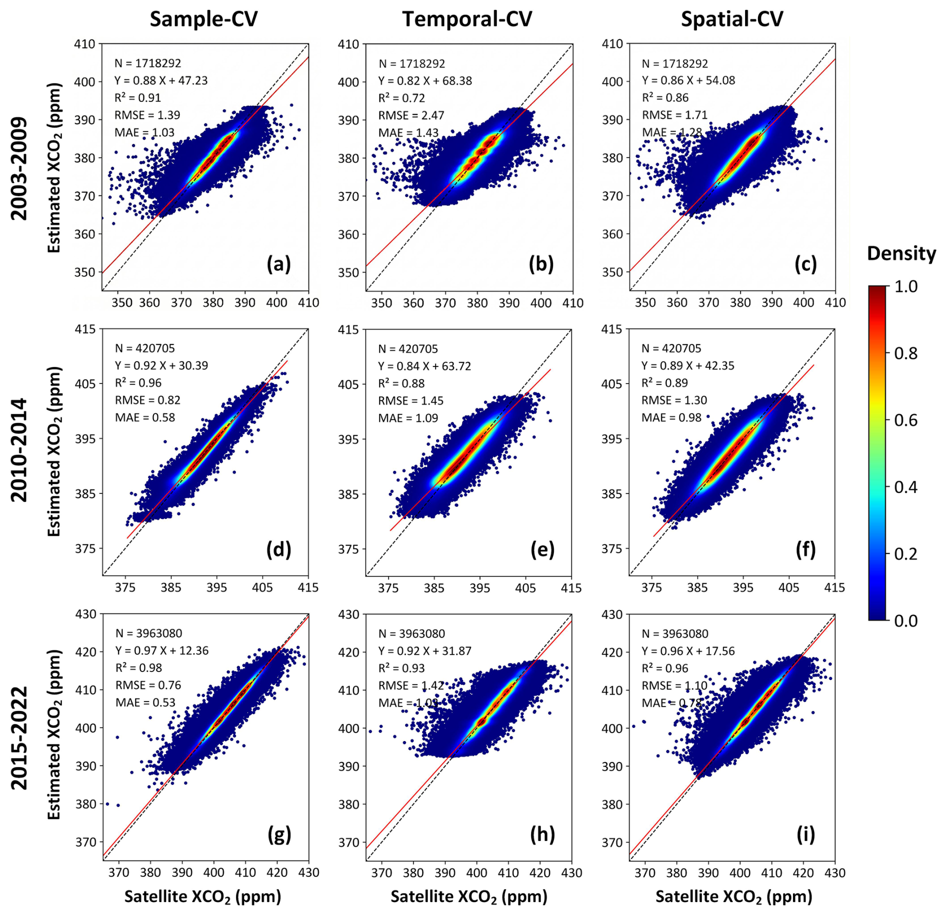
Figure 3 Density scatterplots of sample-based (a, d, g), temporal-based (b, e, h), and spatial-based (c, f, i) ten-fold cross-validation (10-CV) results for daily XCO₂ estimates during 2003–2009 (SCIAMACHY, a–c), 2010–2014 (GOSAT, d–f), and 2015–2022 (OCO-2, g–i). Black dashed lines represent the 1:1 relationship, and red solid lines indicate linear regression fits.

Furthermore, we independently evaluated our data-fused XCO₂ estimates against TCCON ground-based measurements and compared their performance with satellite retrievals and the CAMS reanalysis. Satellite XCO₂ observations show strong agreement with TCCON, yielding an R² of 0.96, an RMSE of 1.67 ppm, and a mean bias of 0.13 ppm (Fig. 4a). CAMS reanalysis exhibits a comparable correlation (R²=0.97) but larger errors and a more pronounced systematic bias (RMSE = 1.74 ppm, mean bias = 0.38 ppm; Fig. 4b). In contrast, our data-fused XCO₂ product achieves the best agreement with TCCON, with an R² of 0.99, an RMSE of 1.10 ppm, an MAE of 0.82 ppm, and a near-zero mean bias of 0.01 ppm (Fig. 4c), demonstrating that the fusion framework substantially improves consistency with ground-based observations.

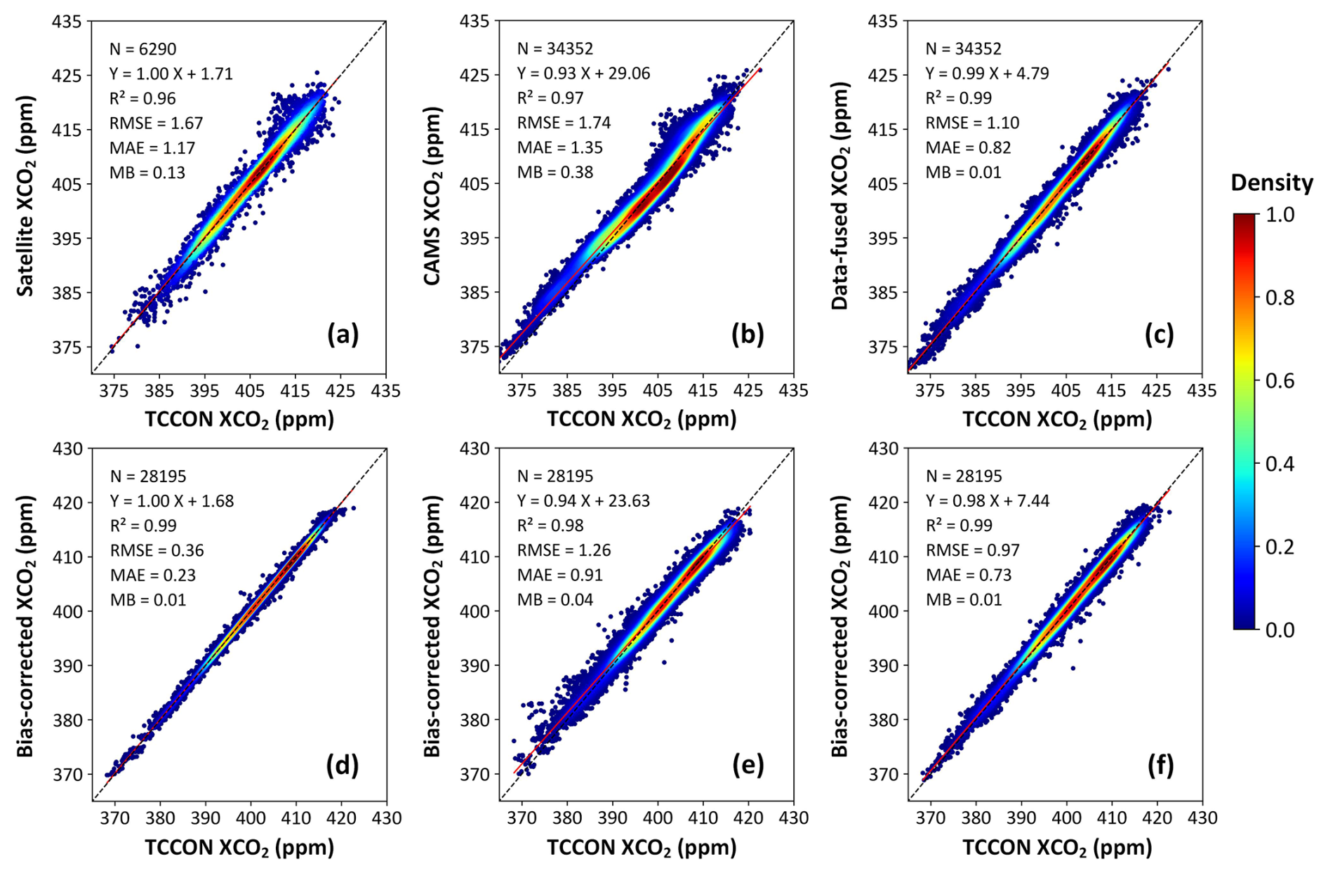
Figure 4 Density scatterplots comparing daily XCO₂ concentrations from (a) satellite retrievals, (b) CAMS reanalysis, and (c) our data-fusion approach against TCCON ground-based measurements, as well as ten-fold cross-validation (10-CV) results for our bias-corrected daily XCO₂ concentrations using (d) sample-based, (e) temporal-based, and (f) spatial-based CV strategies. Black dashed lines represent the 1:1 relationship, and red solid lines indicate linear regression fits.

3.1.2 Validation of bias-corrected XCO₂ estimates

The bias-corrected XCO₂ estimates achieve excellent agreement with TCCON observations (R²=0.99, RMSE = 0.36 ppm, MAE = 0.23 ppm) and a near-zero mean bias of 0.01 ppm, indicating that systematic biases in the data-fused product are effectively removed (Fig. 4d). Temporal-based CV further demonstrates stable predictive performance under interannual extrapolation: when continuous years are withheld from training, the bias-corrected XCO₂ achieves a CV-R² of 0.98, with an RMSE of 1.26 ppm, an MAE of 0.91 ppm, and a mean bias of 0.04 ppm (Fig. 4e), confirming stable temporal generalization across different years. Spatial-based CV confirms strong spatial transferability, with a CV-R² of 0.99, an RMSE of 0.97 ppm, an MAE of 0.73 ppm, and a mean bias of 0.01 ppm (Fig. 4f), demonstrating reliable performance when extrapolating to under-monitored regions.

Beyond overall statistical accuracy, temporal seamlessness is critical when merging multi-decadal satellite records, particularly across mission transitions where systematic retrieval offsets can introduce artificial discontinuities. To evaluate the temporal stability of the reconstructed dataset across major satellite mission transitions (∼2010 and ∼2015), we conducted targeted diagnostics at long-term TCCON sites, including Garmisch (Europe) and Park Falls (North America) (Fig. 5). Daily XCO₂ time series spanning the SCIAMACHY–GOSAT and GOSAT–OCO-2 transitions reveal clear differences between the initial data-fused product and the bias-corrected reconstruction. At both sites, the uncorrected fused XCO₂ occasionally exhibits small but discernible step changes or systematic offsets coincident with mission transitions, indicating residual inter-mission inconsistencies. In contrast, the bias-corrected XCO₂ time series remains temporally smooth and continuous across the transition periods, with no apparent artificial discontinuities. Moreover, the corrected series closely follows TCCON observations in both seasonal phase and amplitude, preserving natural temporal variability while effectively eliminating sensor-induced biases. Together, these results highlight the robustness of the bias-correction strategy in ensuring the temporal seamlessness of the multi-decadal XCO₂ record.

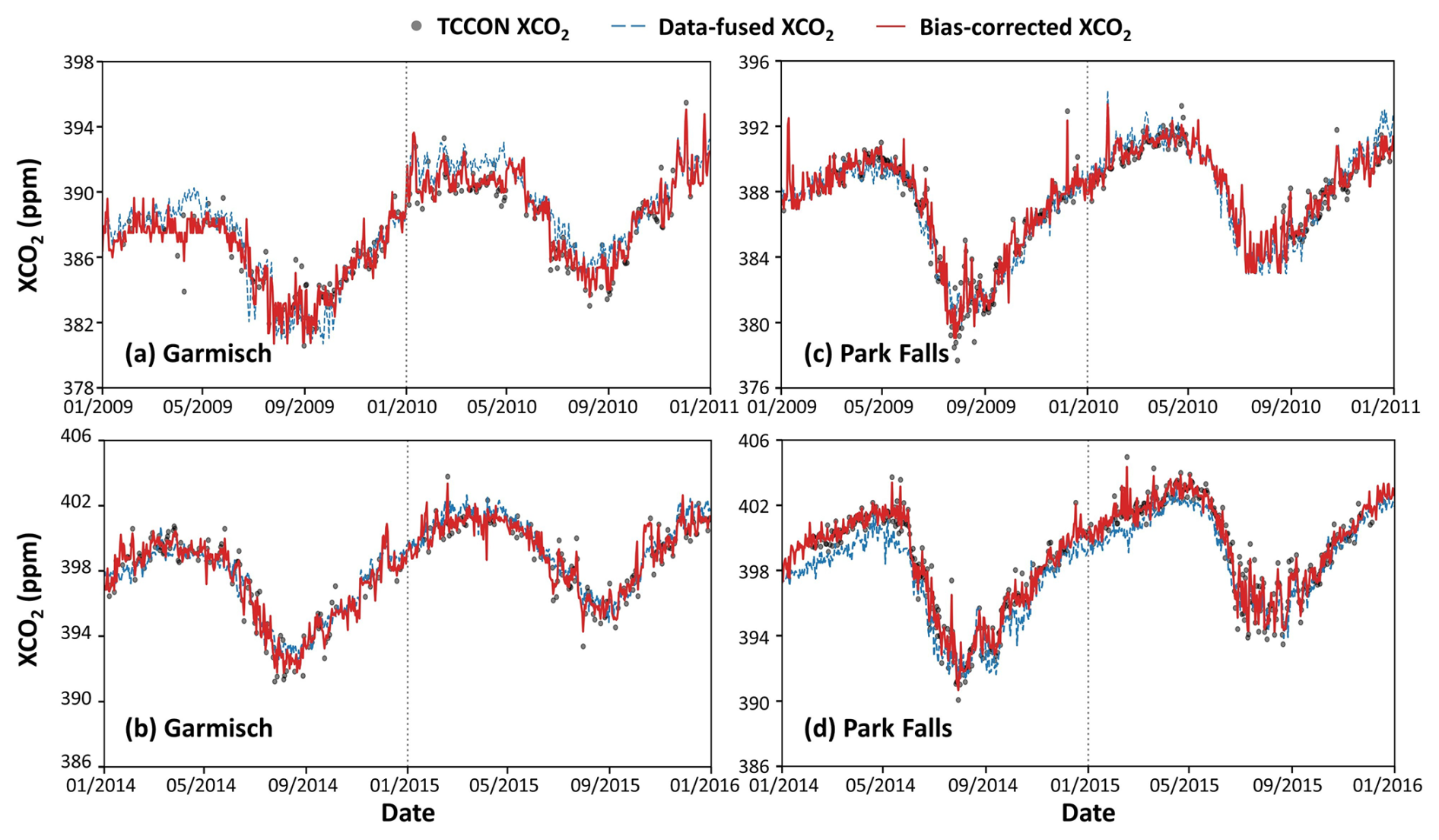
Figure 5 Time series of TCCON (grey dots), data-fused (blue dashed lines), and bias-corrected (red solid lines) XCO₂ concentrations at (a, b) Garmisch (Europe) and (c, d) Park Falls (North America) across major satellite mission transitions: (a, c) SCIAMACHY–GOSAT (2009–2010) and (b, d) GOSAT–OCO-2 (2014–2016). The vertical dotted lines indicate the approximate timing of satellite mission transitions.

3.1.3 Independent validation against ObsPack observations

To further evaluate the generalization ability of the bias-corrected daily XCO₂ dataset, we conducted an independent validation against surface flask measurements at 41 ObsPack stations from 2003 to 2022 (Fig. 6). The bias-corrected XCO₂ exhibits strong consistency with ObsPack observations, yielding a global mean R² of 0.86. More than 90 % of the stations show high R² values exceeding 0.6, and over half (54 %) exceed 0.9, indicating robust performance across diverse geographic and climatic conditions. The low R² at the AZR station is mainly due to the limited number of matched observations and the relatively small temporal variability at this site, which can lead to unstable correlation statistics. Importantly, the RMSE and bias at this station remain relatively small, suggesting that the low R² does not indicate a systematic deficiency in the reconstructed dataset. Spatially, most stations (58 %) show RMSE values ranging from 3 to 6 ppm, with larger values observed at stations in North America, Europe, and East Asia, where complex terrain and strong anthropogenic emissions dominate. Nonetheless, the estimated bias and MAE are generally low, with more than 73 % and 80 % of the stations having bias values within ±3 ppm and MAE values below 5.0 ppm, respectively.

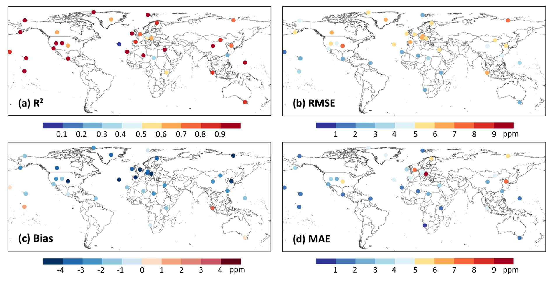
Figure 6 Global validation of our bias-corrected daily XCO₂ dataset against ObsPack surface flask observations during 2003–2022.

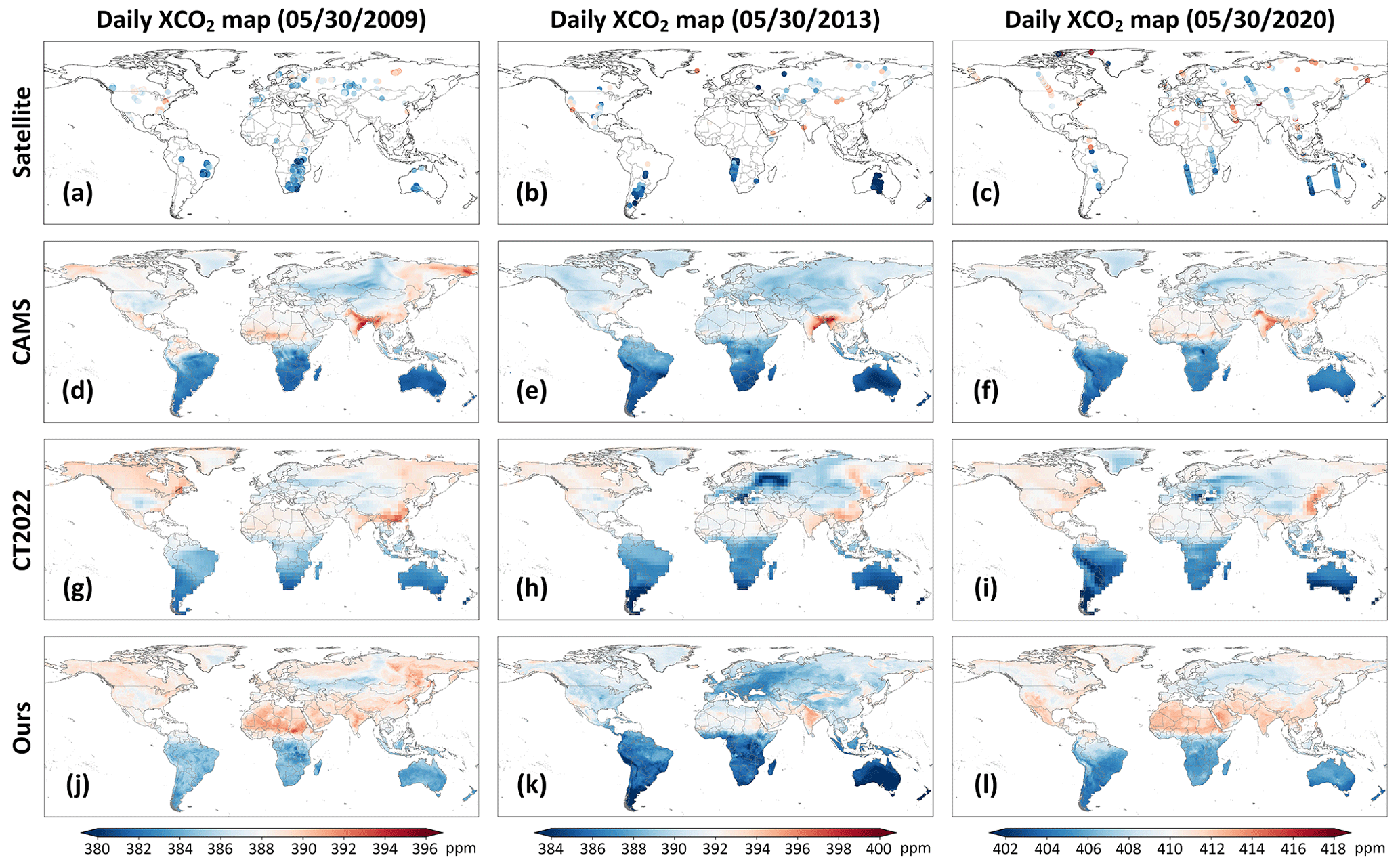
Figure 7 Spatial distributions of global daily XCO₂ concentrations on 30 May 2009, 2013, and 2020 from (a–c) SCIAMACHY, GOSAT, and OCO-2 retrievals, (d–f) CAMS reanalysis, (g–i) CarbonTracker (CT2022), and (j–l) our reconstructed XCO₂ product.

3.2 Spatiotemporal variations of global atmospheric XCO₂

3.2.1 Global daily seamless XCO₂ maps

We compare global daily XCO₂ data derived from different products for three representative dates: 30 May 2009, 2013, and 2020, where the coarser-resolution products are plotted at their native resolutions for qualitative comparison (Fig. 7). Satellite retrievals provide physically realistic XCO₂ signals but suffer from sparse and discontinuous spatial coverage due to orbital limitations and cloud contamination. CAMS (0.75°×0.75°) offers spatially complete fields but tends to weaken local spatial gradients, attenuating enhancements over major emission regions and underestimating background values in the Southern Hemisphere. CarbonTracker 2022 (CT2022, 3°×2°) is a widely used global CO₂ flux inversion system developed by NOAA to quantify atmospheric CO₂ sources and sinks using transport modeling (Jacobson et al., 2023). It captures large-scale interhemispheric gradients but exhibits regional inconsistencies, including exaggerated concentrations in parts of the Northern Hemisphere mid-latitudes and muted contrasts in tropical source regions. In contrast, our XCO₂ product achieves seamless global coverage while preserving fine-scale spatial heterogeneity and maintaining close consistency with satellite retrievals where available. Representative regional comparisons (highlighted by red circles) further illustrate these differences. In 2009, CT2022 overestimated XCO₂ concentrations over the eastern United States, while CAMS underestimated regional XCO₂ enhancements; our estimates closely matched satellite observations. In 2013, both CAMS and CT2022 underestimated XCO₂ concentrations over northern China and southern Mongolia, whereas our product accurately captured the observed spatial patterns. In 2020, both CAMS and CT2022 underestimated XCO₂ concentrations over the Middle East, whereas our reconstruction captured the enhanced concentrations, in agreement with satellite observations. These examples demonstrate that our data provide a balanced and physically consistent representation of daily global XCO₂, avoiding CAMS over-smoothing and the regional biases evident in CT2022.

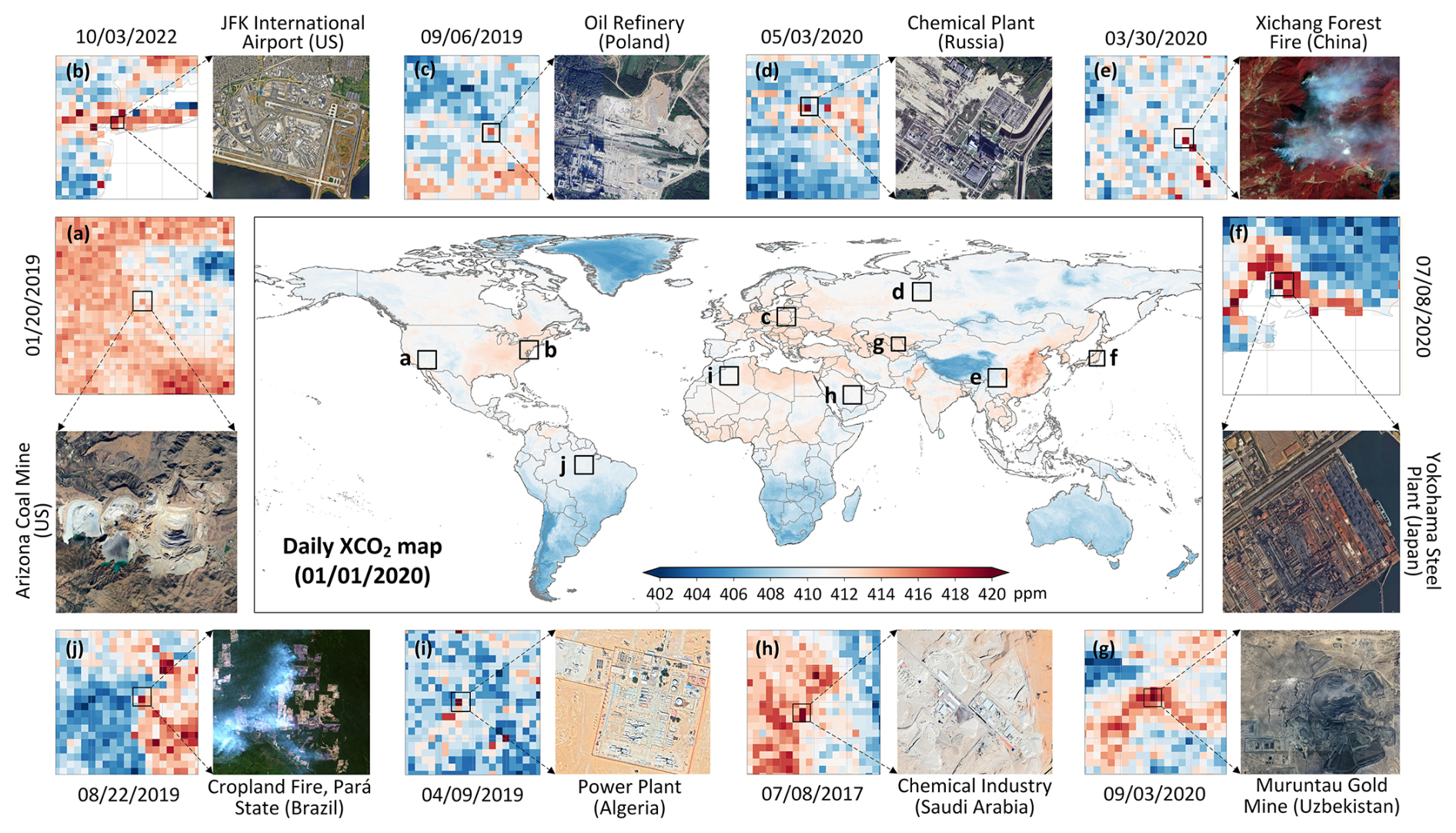
Figure 8 Characterization of localized XCO₂ enhancement identified signals from the reconstructed global daily seamless dataset across (a–j) 10 regions of interest on different days. The central map shows the global distribution of XCO₂ on 1 January 2020.

3.2.2 Characterization of localized XCO₂ enhancement signals

Daily XCO₂ observations provide a distinct advantage for revealing localized and transient regions with elevated XCO₂ concentrations that are often obscured in temporally averaged products (Fig. 8). Pronounced XCO₂ enhancements are observed over regions with strong anthropogenic influence, including major industrial and energy-related areas such as steel production (the Yokohama Steel Plant in Japan), coal mining (the Arizona Coal Mine in the US), power generation (a power plant in Algeria), and chemical processing (a chemical plant in Russia). Elevated XCO₂ concentrations are also observed over industrial clusters in East Asia, Central Asia (the Muruntau Gold Mine in Uzbekistan), Europe (an oil refinery in Poland), North America, and the Middle East (the chemical industry in Saudi Arabia). These patterns are consistent with localized regions of relatively high XCO₂ concentrations associated with fossil-fuel combustion and extraction-related activities. In addition to stationary sources, localized enhancements are also evident near major transport hubs, such as John F. Kennedy International Airport in the US. Beyond anthropogenic sources, the daily XCO₂ dataset also captures episodic enhancement events associated with natural processes, such as forest fires (the Xichang Forest Fire in China) and large-scale agricultural burning (cropland fires in Pará State, Brazil), which can generate short-lived yet spatially coherent XCO₂ anomalies at daily timescales. These examples suggest that the reconstructed daily XCO₂ product can identify typical regions with elevated XCO₂ concentrations associated with both anthropogenic and natural processes, resolve their spatial footprints, and support the monitoring of regional XCO₂ variability at the global scale. Nevertheless, these selected examples are intended to illustrate localized elevated XCO₂ signals rather than strict point-source detections; however, some isolated high-value pixels may partly reflect retrieval uncertainty or noise, especially in regions with limited observations.

3.2.3 Impacts of biomass burning and ENSO on XCO₂ growth

Elevated fire-related CO₂ emissions and corresponding short-term XCO₂ anomalies are clearly captured in our reconstructed dataset during extreme wildfire events. Over southeastern Australia (Fig. 9a), pronounced XCO₂ enhancements are observed from 27 December 2019, to 8 January 2020, coinciding with the peak of the 2019–2020 Australian bushfires. The daily XCO₂ time series exhibits a distinct local maximum on 5 January 2020 (average = 411.35±0.56 ppm), superimposed on a gradually increasing background trend, with spatial distributions revealing significantly elevated concentrations over fire-affected regions. A similar short-term response is detected over Xichang City in southwestern China during the March–April 2020 wildfire episode (Fig. 9b), lasting for over two weeks, from 24 March to 8 April 2020, with elevated daily XCO₂ concentrations. A clear local peak of 410.56±0.53 ppm is observed on 30 March, coinciding with the reported Xichang forest fire outbreak, followed by a gradual decline after 5 April. These event-scale XCO₂ anomalies, resolved at daily resolution, demonstrate the dataset's ability to capture rapid, short-lived carbon emissions and their impact on regional atmospheric XCO₂ variability.

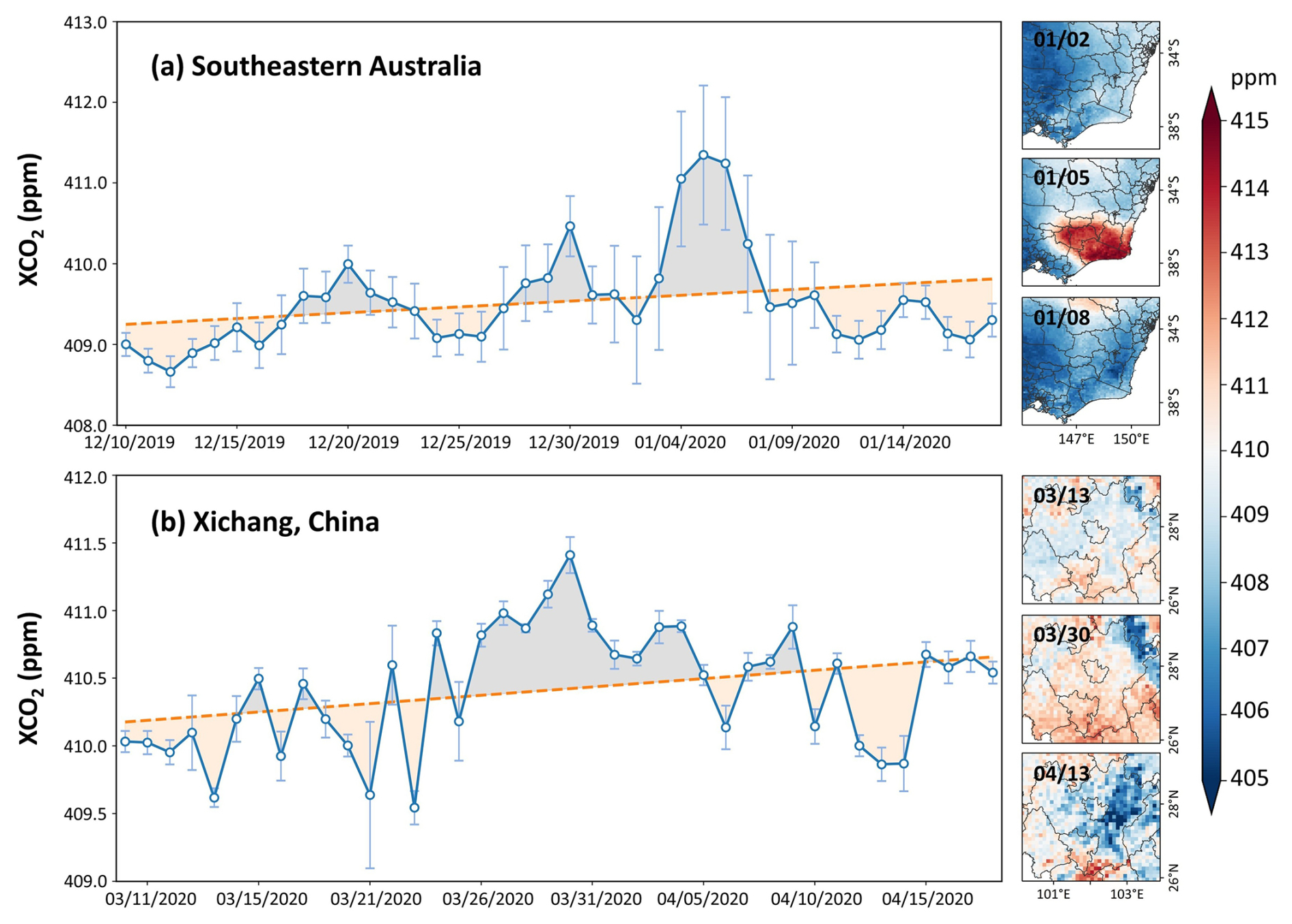
Figure 9 Time series and spatial distributions of daily XCO₂ concentrations associated with extreme wildfire events in (a) southeastern Australia during December 2019–January 2020 and (b) Xichang, China, during March–April 2020.

Figure 10 shows that XCO₂ growth rates from our reconstructed dataset consistently respond to ENSO phases, as evidenced by a strong correlation with the multivariate ENSO index (MEI; R=0.55, p<0.01) (Wolter and Timlin, 2011), which explains ∼30 % of the observed interannual variability (Kim et al., 2016; Chatterjee et al., 2017). ENSO-driven anomalies in temperature and precipitation strongly regulate terrestrial carbon uptake and fire activity (da Costa et al., 2024). During El Niño conditions, warmer, drier climates suppress ecosystem CO₂ uptake and enhance biomass burning, leading to elevated atmospheric growth rates (Betts et al., 2016; Guan et al., 2023; Ak-Bhd, 2021). This effect was most evident during the extreme 2015–2016 El Niño, which coincided with the highest recorded global XCO₂ growth rate of 3.11 ppm yr⁻¹ (p<0.001) (Liu et al., 2024). In contrast, La Niña phases are typically associated with cooler and wetter conditions that strengthen terrestrial carbon sinks and reduce atmospheric CO₂ growth rates, as observed in 2011–2012 and 2022 (Wang et al., 2014; Chatterjee et al., 2017). Regionally, ENSO sensitivity is highest in the tropics, where MEI explains ∼45 % of the interannual variability, highlighting the vulnerability of tropical forests to climate-induced stress and fire-related carbon losses (Brando et al., 2019; Liu et al., 2022). The Northern Extratropics show moderate sensitivity (∼37 %), while the Southern Extratropics are less affected (∼27 %), reflecting hemispheric differences in land–atmosphere coupling and fire regimes.

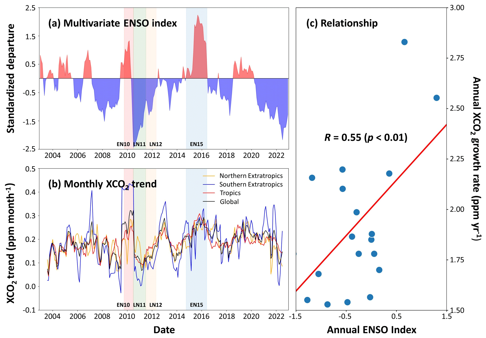
Figure 10 Time series of the monthly (a) multivariate ENSO index and (b) detrended XCO₂ growth rates over major regions, including the Northern Extratropics (30–90° N), Southern Extratropics (90–30° S), Tropics (30° S–30° N), and the globe. (c) Scatter plots of annual XCO₂ growth rates versus the annual ENSO index. The 2011 La Niña event (LN11) is shaded in dark green. The preceding 2010 El Niño event (EN10) and subsequent weak 2012 La Niña event (LN12) are shaded in lighter red and green colors, respectively. The 2015 El Niño event (EN15) is shaded in dark blue.

3.2.4 Annual maps and long-term trends in global XCO₂

Figure 11 shows the annual mean global XCO₂ from 2003 to 2022 over land, revealing a pronounced and sustained increase over the past two decades. During the early period (2003–2005), global XCO₂ levels were relatively low, with most regions characterized by concentrations below ∼380 ppm. From 2006 to 2010, XCO₂ increased steadily across all continents, while spatial contrasts remained relatively modest. After approximately 2010, the spatial patterns intensified markedly. From 2011 to 2015, high-XCO₂ regions expanded and strengthened, and from 2016 onward, the global increase accelerates further, with XCO₂ exceeding ∼410 ppm over large portions of the Northern Hemisphere by 2018–2019 (Buchwitz et al., 2018; Lee et al., 2025). By 2022, nearly all continental regions displayed XCO₂ values above 415 ppm, with the highest concentrations concentrated over major industrialized and densely populated regions in the Northern Hemisphere. Overall, the global mean XCO₂ increased monotonically from 374.54 ppm in 2003 to 416.36 ppm in 2022, corresponding to approximately an 11 % increase over the past 20 years. This substantial growth highlights the rapid accumulation of atmospheric CO₂ and the growing influence of anthropogenic emissions on the global carbon cycle.

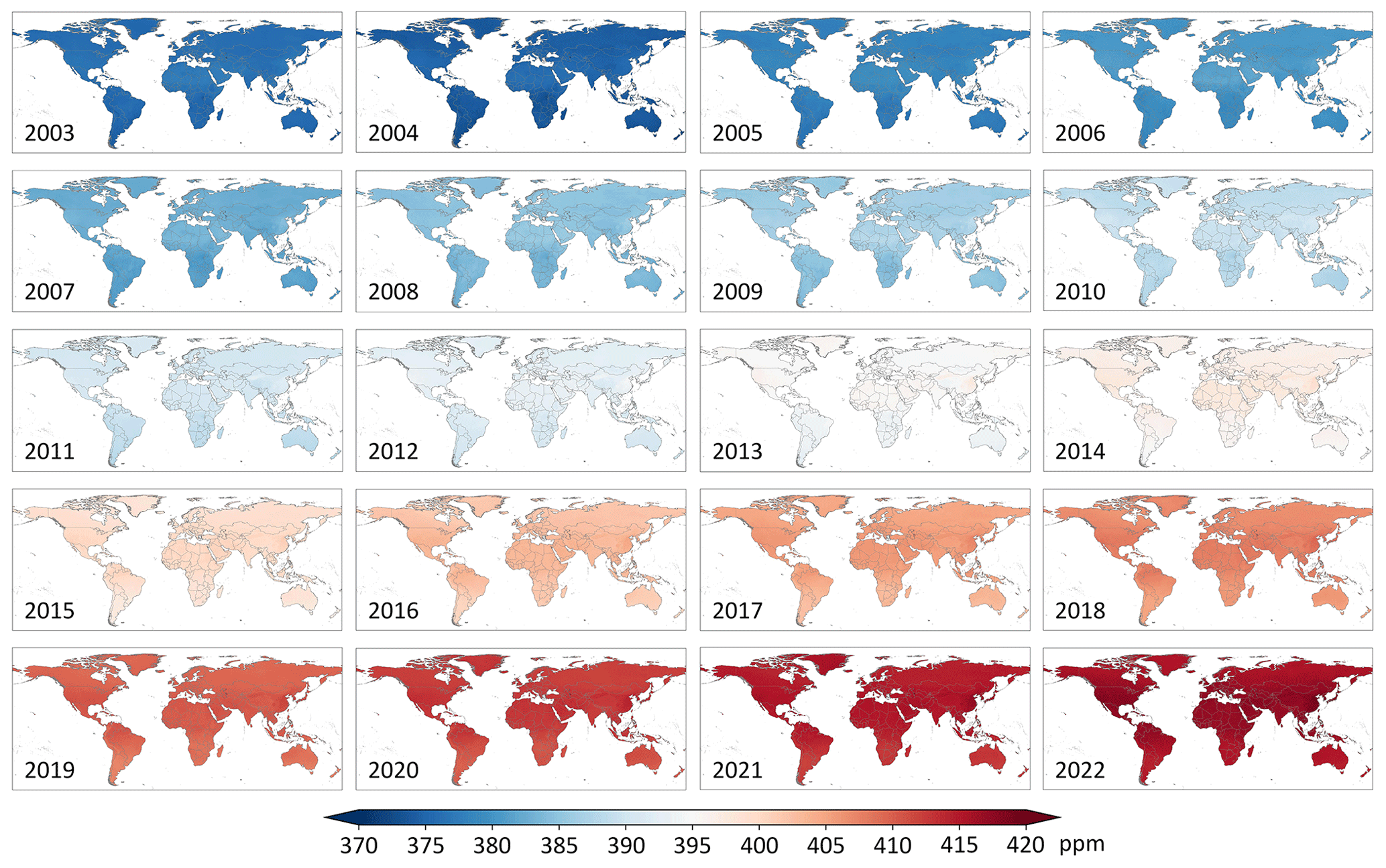
Figure 11 Spatial distribution of annual mean XCO₂ concentrations (unit: ppm) over land from 2003 to 2022.

Figure 12 presents the long-term (2003–2022) annual mean XCO₂ and seasonal climatology. The long-term global mean XCO₂ is 394.58±0.76 ppm, with a clear interhemispheric gradient, characterized by higher concentrations in the Northern Hemisphere and lower values in the Southern Hemisphere. The highest XCO₂ concentrations are concentrated in the northern low- to mid-latitudes (∼10–45° N), encompassing East and Southeast Asia, northern Africa and the Middle East, the United States, and parts of Europe and South Asia. These regions coincide with dense population centers, intensive industrial activity, and high fossil fuel consumption (Crippa et al., 2021; Sheng et al., 2021). Conversely, persistently low XCO₂ values occur over South America, central and southern Africa, and Australia, where strong biospheric uptake, sparse anthropogenic emissions, and the influence of clean marine air masses suppress atmospheric CO₂ levels. At the national scale, South Korea exhibits the highest XCO₂ value (396.11±0.69 ppm), followed by Kuwait (395.88±0.79 ppm), consistent with intensive energy use and strong fossil fuel dependence.

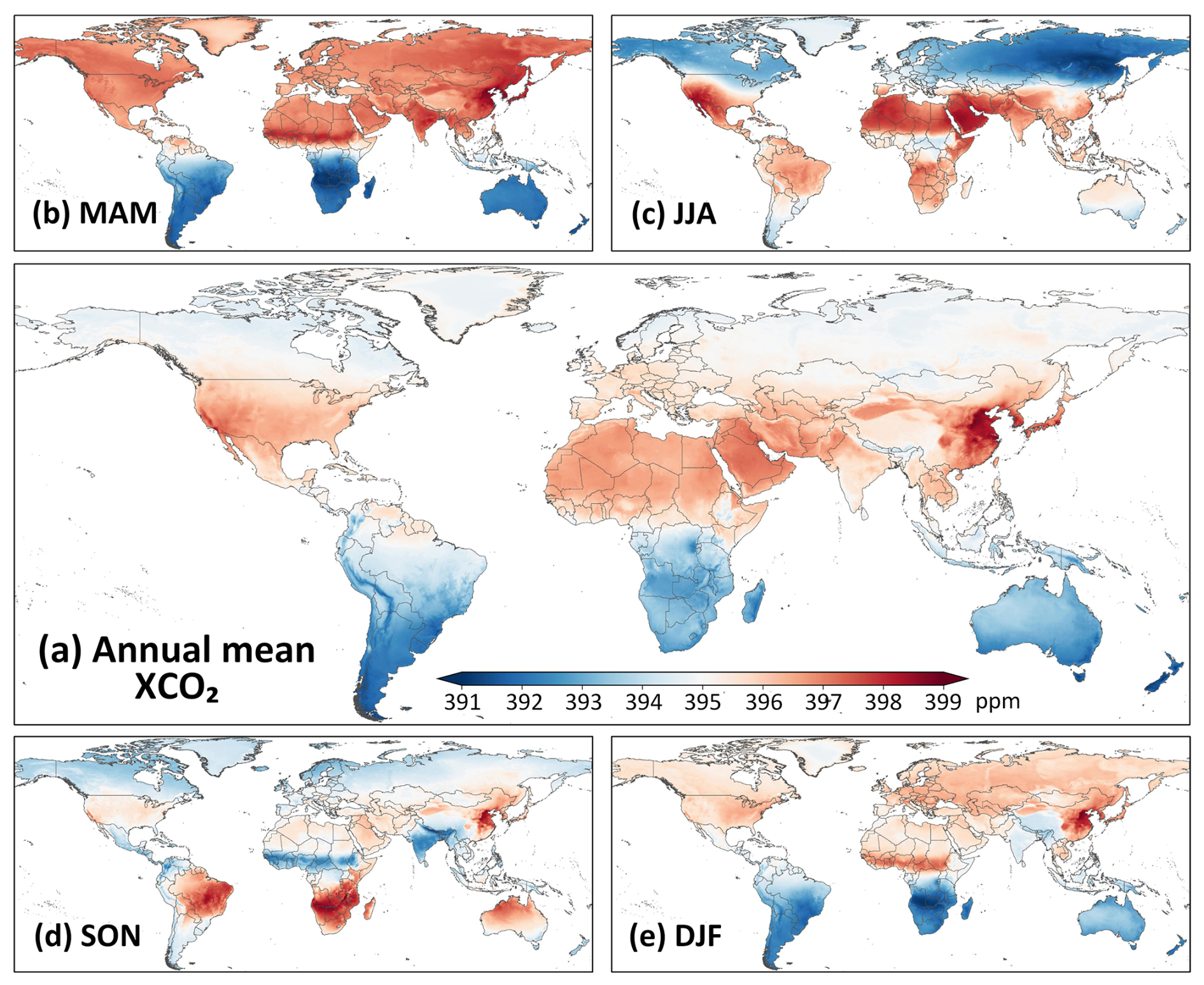
Figure 12 Multi-year (a) annual mean XCO₂ map (unit: ppm) over land for 2003–2022 and seasonal mean XCO₂ maps for (b) March–April–May (MAM), (c) June–July–August (JJA), (d) September–October–November (SON), and (e) December–January–February (DJF).

Pronounced seasonal variability in XCO₂ is evident across global land (Fig. 12b–d). During boreal spring (MAM; average = 395.36±2.20 ppm), elevated XCO₂ concentrations are widespread across the Northern Hemisphere, reflecting accumulated winter emissions and the delayed onset of biospheric uptake. In boreal summer (JJA; average = 392.74±1.29 ppm), XCO₂ decreases markedly over northern high-latitude continents but increases in the Southern Hemisphere, forming extensive low-concentration bands associated with peak vegetation photosynthesis and strong net carbon uptake. Boreal autumn (SON; average = 393.48±0.54 ppm) is characterized by distinct enhancements over southern Africa, South America, and much of Australia, linked to biomass burning and reduced biospheric uptake. Seasonal amplitudes are particularly large in East Asia and the western United States (e.g., California), where intensive anthropogenic emissions coincide with strong biospheric seasonality (Sheng et al., 2021; Guan et al., 2024). In boreal winter (DJF; mean = 394.76±1.37 ppm), enhanced fossil fuel combustion and reduced biospheric uptake lead to elevated XCO₂ concentrations across the Northern Hemisphere, whereas lower values prevail over the Southern Hemisphere land and adjacent oceans, resulting in a pronounced interhemispheric gradient.

Figure 13 presents long-term XCO₂ trends from 2003 to 2022 across different temporal scales. All land regions exhibit significant increasing trends, with an average of 2.24 ppm yr⁻¹ (p<0.001). The strongest increases (>2.25 ppm yr⁻¹) occur over East and Southeast Asia, northern South America, and central Africa, while comparatively weaker growth (<2.15 ppm yr⁻¹) is observed over southern South America, Australia, and the Sahara. Seasonal trends reveal distinct patterns (Fig. 13b–e). During MAM (average = 2.16 ppm yr⁻¹, p<0.001), large positive trends dominate the northern mid-latitudes, especially across much of Asia and North America, reflecting winter-emission accumulation and delayed biospheric uptake. In JJA (average = 2.23 ppm yr⁻¹, p<0.001), trends weaken over boreal and temperate regions but remain pronounced in the tropics, particularly in the Amazon basin, central Africa, and Southeast Asia, reflecting ongoing anthropogenic emissions and biomass burning. SON (average = 2.25 ppm yr⁻¹, p<0.001) shows enhanced trends over Africa and South America, forming clear regional maxima in biomass-burning regions, while northern mid-latitudes experience moderate growth. In DJF (average = 2.19 ppm yr⁻¹, p<0.001), trends intensify again across the Northern Hemisphere, notably in East Asia and Europe, driven by wintertime fossil fuel combustion, whereas the Southern Hemisphere shows weaker increases. Although the spring and winter seasons exhibit stronger regional contrasts, the autumn season shows a systematically higher spatially averaged XCO₂ growth trend, indicating a more widespread enhancement rather than localized extremes.

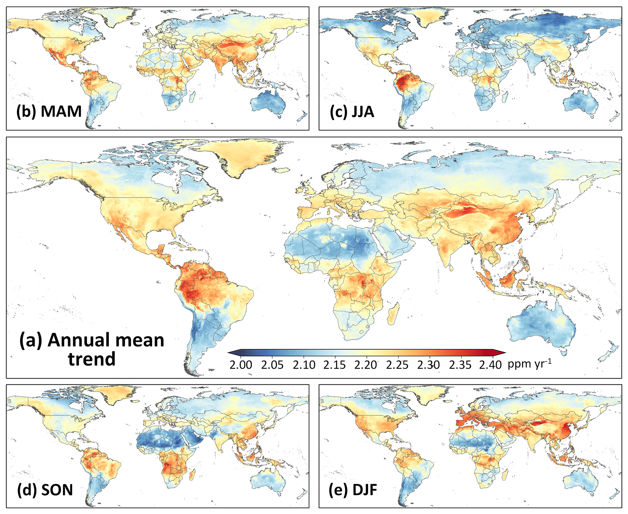
Figure 13 Spatial patterns of long-term (a) annual XCO₂ trends (unit: ppm yr⁻¹) from 2003 to 2022 and seasonal XCO₂ trends (unit: ppm yr⁻¹) for (b) March–April–May (MAM), (c) June–July–August (JJA), (d) September–October–November (SON), and (e) December–January–February (DJF).

3.3 Discussion

3.3.1 Model interpretation with XAI

To improve model transparency and quantify the relative importance of input variables, we applied SHapley Additive exPlanations (SHAP) to the trained spatiotemporal Transformer–BiLSTM model (Lundberg and Lee, 2017). The SHAP values were calculated to assess the contribution of each predictor to the reconstructed XCO₂ fields. For the data-fusion stage (Fig. 14a), CAMS XCO₂ emerges as the dominant contributor, accounting for 37 % of the total importance, reflecting its role in providing a temporally continuous and spatially coherent background field. Spatiotemporal encoding variables collectively contribute 30 %, highlighting the importance of explicitly representing spatial structure and temporal dynamics in global XCO₂ reconstruction. Meteorological variables (16 %) and satellite-derived surface variables (11 %) provide complementary information that refines regional-scale variability, while precursor gases contribute a smaller but non-negligible share (6 %). The relatively small mean SHAP value for NO₂ suggests that its overall contribution to the global XCO₂ reconstruction is smaller than that of variables such as CAMS XCO₂ and meteorological factors. This is expected because NO₂ mainly reflects localized anthropogenic combustion emissions, whereas large-scale atmospheric transport, background concentration fields, and biospheric exchange processes more strongly control XCO₂ variability at the global scale. Nevertheless, NO₂ still provides useful complementary information for identifying regional anthropogenic emission patterns, particularly over urban and industrial areas.

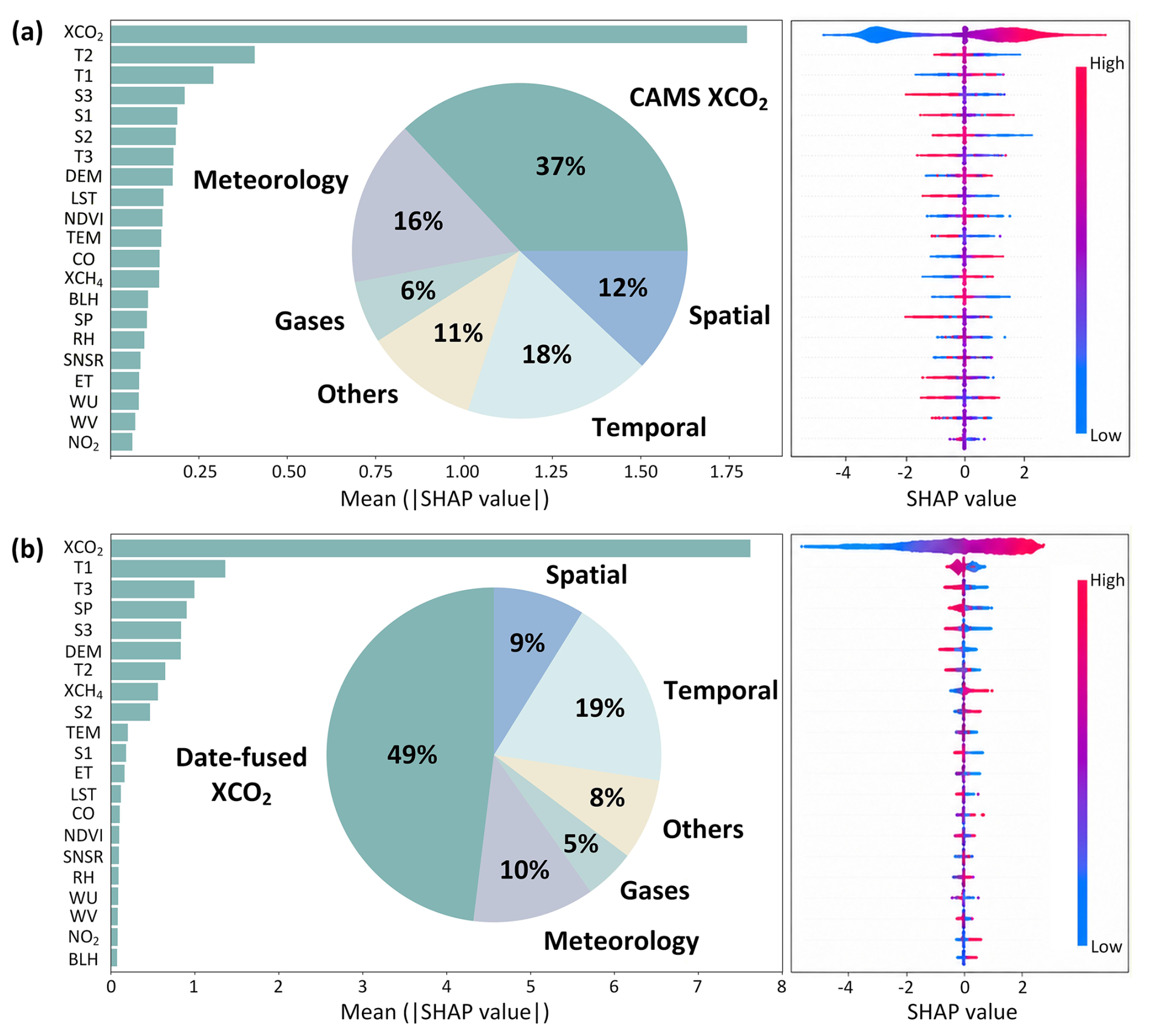
Figure 14 Model interpretability analysis using the SHAP approach, showing the relative importance of each predictor in the (a) data-fusion phase and (b) bias-correction phase.

For the bias-correction stage (Fig. 14b), the fused XCO₂ field dominates the model output, contributing 49 %, consistent with its role as the primary constraint for harmonizing inter-satellite differences using TCCON observations. Temporal indicators (19 %), spatial variables (9 %), and meteorological variables (10 %) further capture systematic temporal, spatial, and environmental patterns in satellite retrieval biases. Overall, the XAI analysis indicates that the proposed framework is primarily constrained by physically meaningful background information, while auxiliary variables are effectively integrated to refine spatiotemporal XCO₂ structures and reduce systematic biases.

3.3.2 Comparison with previous studies

We compared our reconstructed XCO₂ dataset with previous global studies that applied independent validation against TCCON observations (Table 3). Some studies are limited to coarser temporal resolutions at monthly (Zhang et al., 2023; Wang et al., 2025; Hwang et al., 2026; Yu et al., 2026), 8 d (Li et al., 2022; Guan et al., 2024), or 3 d (Sheng et al., 2023) scales, which limits their ability to capture short-term (daily) variability. In addition, many studies generated XCO₂ at coarser spatial resolutions (≥0.25°), limiting their representation of localized emission gradients and subregional heterogeneity (Li et al., 2022; Sheng et al., 2023; Jin et al., 2022; Gao et al., 2023; Huang et al., 2024b; Wang et al., 2023). Many products cover only limited periods (usually <10 years) after 2014, constraining analyses of long-term historical trends (Sheng et al., 2023; Huang et al., 2024b; Li et al., 2026; Lee et al., 2025; Yu et al., 2026). More importantly, previous studies with fine temporal resolution (daily or subdaily) exhibit greater fluctuations in overall accuracy, with R² ranging from 0.91 to 0.98 and RMSE values from 1.06 to 2.62 ppm. However, a recent study (Wang, 2026) provides a long-term global daily XCO₂ product at a 1 km spatial resolution with considerable accuracy (R²=0.98, RMSE = 1.10 ppm). In contrast, our Transformer–BiLSTM framework reconstructs a global, seamless, cross-mission-consistent, daily XCO₂ dataset at 0.1° spatial resolution over 2003–2022, achieving an R² of 0.99 and an RMSE of 1.10 ppm, comparable to or better than those reported in the literature.

Table 3 Comparison of reconstructed global XCO₂ datasets reported in previous studies.

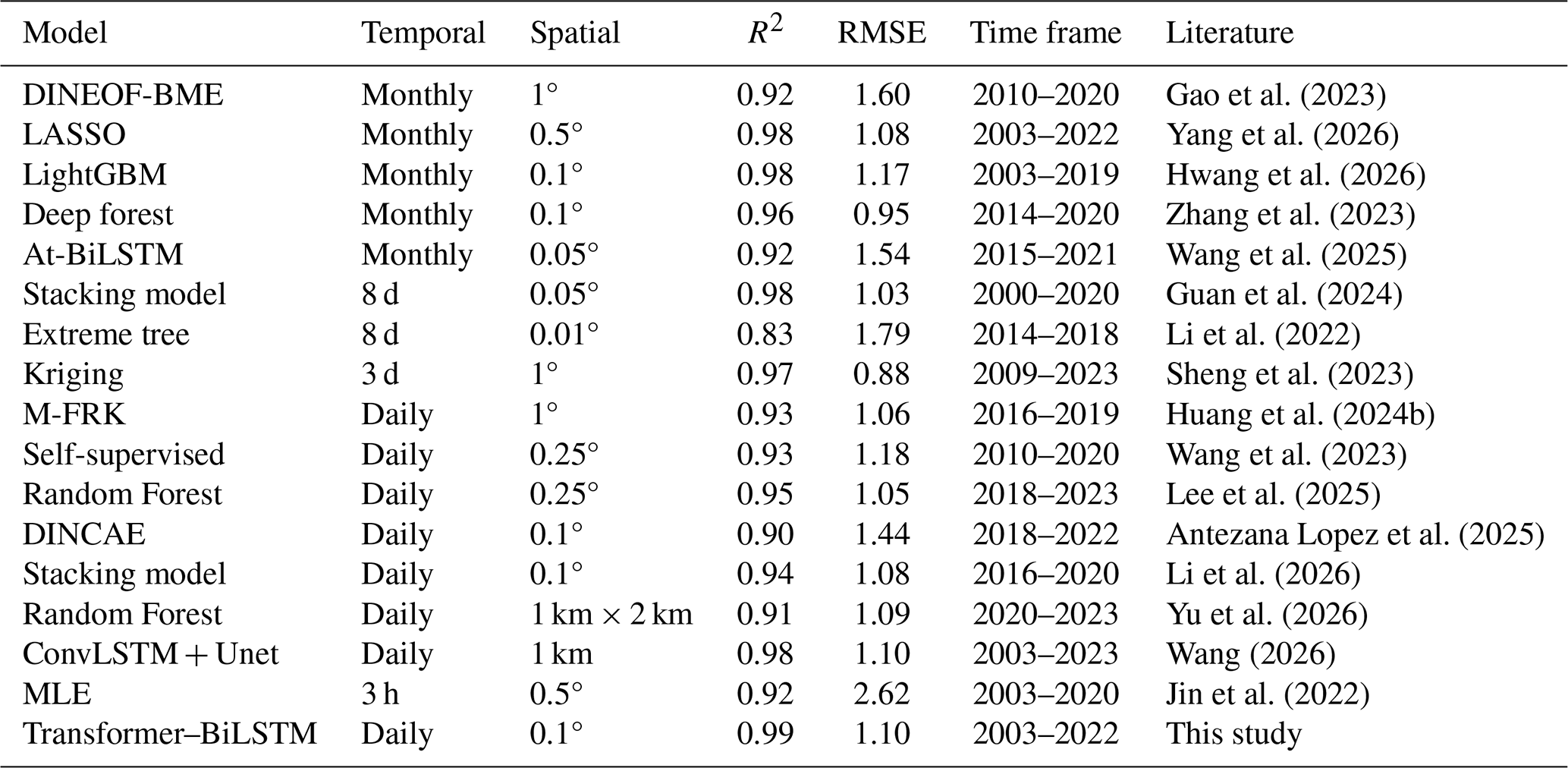
DINEOF-BME: Data Interpolation Empirical Orthogonal Function-Bayesian Maximum Entropy; At-BiLSTM: Attention bidirectional long short-term memory; LASSO: Least Absolute Shrinkage and Selection Operator (LASSO) regression; M-FRK: Multiscale fixed rank kriging; DINCAE: Data Interpolating Empirical Orthogonal Functions and Convolutional Auto-Encoder; MLE: Maximum likelihood estimation.

3.3.3 Strengths

We acknowledge the previous related studies, including Wang (2026), which provides a 1 km global XCO₂ product with strong validation performance. However, our study focuses on constructing a temporally seamless, cross-mission-consistent, and physically coherent daily global XCO₂ dataset spanning two decades (2003–2022), which is particularly important for long-term carbon-cycle and climate analyses, rather than simply pursuing the highest spatial resolution.

The primary innovation of our study lies in the explicit treatment of inter-satellite inconsistencies among SCIAMACHY, GOSAT, and OCO-2. Previous long-term reconstruction studies generally fuse multiple satellite products directly but often do not sufficiently address systematic biases arising from differences in sensor characteristics, orbital sampling, retrieval algorithms, and mission transitions. These inconsistencies can introduce artificial discontinuities and temporal drift, compromising long-term trend analyses. To address this issue, we developed a TCCON-guided bias-correction framework that harmonizes observations across different satellite missions and minimizes artificial step changes during the SCIAMACHY–GOSAT and GOSAT–OCO-2 transition periods. Compared with the uncorrected data-fused product, the bias-corrected XCO₂ dataset exhibits improved agreement with TCCON, with RMSEs of 0.36, 1.26, and 0.97 ppm under sample-based, temporal-based, and spatial-based ten-fold cross-validation, respectively. These findings highlight the importance of cross-mission harmonization for constructing consistent and reliable long-term XCO₂ records.

Another key strength of our study is the emphasis on temporal continuity and daily dynamics. While previous studies mainly focus on improving spatial resolution, our hybrid Transformer–BiLSTM framework is specifically designed to capture both long-range spatial dependencies and temporal evolution. The Transformer module leverages self-attention mechanisms to characterize non-local spatial relationships and global contextual information, while the BiLSTM module extracts temporal features to preserve daily continuity and capture temporal evolution. In addition, we introduced a weighted spatiotemporal loss function to jointly constrain point-wise accuracy, temporal smoothness, and spatial coherence. These designs enable the reconstruction of seamless daily XCO₂ fields while better capturing temporal variability driven by atmospheric transport, biospheric carbon exchange, and anthropogenic emissions.

Importantly, our study also places a stronger emphasis on physical interpretability. In addition to satellite XCO₂ observations, we incorporate multiple physically relevant predictors, including CAMS XCO₂, meteorological variables, surface variables, and emission-related precursor gases such as NO₂, CO, and XCH₄. These variables help characterize atmospheric circulation, fossil-fuel combustion, biomass burning, and biospheric activity, thereby improving the physical realism of the reconstructed XCO₂ fields. SHAP analysis further confirms the meaningful contribution of these predictors to the reconstruction process. We believe this is an important advantage because high spatial resolution alone cannot compensate for missing physical constraints or temporal inconsistencies.

Furthermore, our validation framework is more comprehensive for assessing long-term robustness. In addition to evaluation against TCCON observations, we also validate the dataset using 41 independent ObsPack stations distributed globally. These independent evaluations demonstrate that the reconstructed dataset maintains strong spatial transferability and temporal stability across diverse regions and atmospheric conditions.

Therefore, the novelty of our study lies not in generating another high-resolution XCO₂ dataset but in developing a temporally seamless, physically consistent, and cross-satellite-harmonized daily global XCO₂ record suitable for investigating long-term carbon-cycle dynamics, interannual variability, and climate-related changes. In this regard, our dataset complements previous ultra-high-resolution products (Wang, 2026), which emphasize fine-scale spatial mapping, by providing a framework optimized for long-term temporal analyses and climate applications that require stable cross-mission continuity.

4 Data availability

The daily high-resolution seamless global XCO₂ product (GlobalHighXCO₂) is publicly available at https://doi.org/10.5281/zenodo.18220962 (Qu and Wei, 2026).

5 Conclusions

Accurate, high-resolution observations of atmospheric XCO₂ are critical for understanding the global carbon cycle, quantifying anthropogenic emissions, and supporting climate mitigation strategies. This study develops a novel Transformer–BiLSTM framework to reconstruct a global, daily, and spatially seamless XCO₂ dataset over land at 0.1° resolution covering 2003–2022. By jointly integrating multi-mission satellite retrievals, CAMS reanalysis, meteorological variables, and precursor gas information, the framework effectively bridges spatial gaps and temporal discontinuities inherent in individual satellite records. A dedicated spatiotemporal loss formulation enforces continuity across space and time, and a bias-correction strategy harmonizes inter-satellite differences to generate a physically consistent long-term XCO₂ record.

Comprehensive validation demonstrates that the reconstructed dataset achieves high accuracy and robustness, as evidenced by independent evaluation against TCCON observations after data fusion (R²=0.99, RMSE = 1.10 ppm), and sample-based ten-fold cross-validation after bias correction (CV-R²=0.99, RMSE = 0.36 ppm). The daily XCO₂ dataset enables the detection of rapid temporal variations and the characterization of localized XCO₂ enhancement patterns associated with a wide range of emission sources, including urban activities, industrial emissions, and biomass burning. The dataset also effectively captures strong responses of XCO₂ growth to major climate events, such as intense El Niño episodes and large-scale wildfires. Across temporal scales, XCO₂ increased significantly at a global mean rate of approximately 2.24 ppm yr⁻¹ (p<0.001) from 2003 to 2022. Spatially, the largest growth rates occurred over northern South America, East and Southeast Asia, and central Africa, while relatively weaker increases were observed over southern South America, Australia, and the Sahara. This high-resolution, daily global land XCO₂ dataset provides a robust tool for analyzing both long-term trends and short-term variability, offering valuable insights for carbon-cycle research, emission monitoring, and climate mitigation assessments. Future improvements may include enhancing XCO₂ retrievals using higher-resolution satellite observations, better representing natural and, in particular, urban emissions, and expanding ground-based validation networks.