Ice thickness and subglacial topography of Swedish reference glaciers revealed by radio-echo sounding

Sweden currently hosts around 270 glaciers, four of which belong to the 61 reference glaciers monitored worldwide. Eight Swedish glaciers disappeared during the warm summer of 2024, and under the global warming scenario associated with current climate policies, all four Swedish reference glaciers (Mårmaglaciären, Storglaciären, Rabots glaciär, and Riukojietna) are projected to vanish within this century. Such change will have implications for people, ecosystems, infrastructure, and local meteorological processes, highlighting the need to better constrain the resultant emerging post-glacial landscapes. During 2024–2025, we conducted radio-echo sounding (RES) surveys on the four Swedish reference glaciers and obtained a total of 38 205 ice thickness point measurements. The mean measured ice thicknesses are 98 ± 14.5 m for Mårmaglaciären, 90 ± 14.6 m for Storglaciären, 85 ± 14.1 m for Rabots glaciär, and 35 ± 7.9 m for Riukojietna. The corresponding maximum measured ice thicknesses are 241, 225, 158, and 88 m, respectively. The RES-derived ice thickness measurements were used to produce high-resolution (10 × 10 m) maps of ice thickness distribution and subglacial topography for each reference glacier. The resulting mean distributed ice thicknesses and ice volumes are 96 m and 0.32 km³ (Mårmaglaciären), 85 m and 0.25 km³ (Storglaciären), 72 m and 0.23 km³ (Rabots glaciär), and 34 m and 0.10 km³ (Riukojietna), respectively. The RES data for the four reference glaciers are available at https://doi.org/10.17043/tarfala-marma-res-survey-2, https://doi.org/10.17043/tarfala-storglaciaren-res-survey-2, https://doi.org/10.17043/tarfala-rabot-res-survey-2, and https://doi.org/10.17043/tarfala-rivgojiehkki-res-survey-2 (Wang et al., 2026e, f, g, h). The ice thickness and subglacial topography for the four reference glaciers are available at https://doi.org/10.17043/tarfala-marma-res-3, https://doi.org/10.17043/tarfala-storglaciaren-res-3, https://doi.org/10.17043/tarfala-rabot-res-3, and https://doi.org/10.17043/tarfala-rivgojiehkki-res-3 (Wang et al., 2026a, b, c, d).

1 Introduction

Observations of glacier change over the last century show that glaciers are retreating and losing mass at an accelerating rate globally (Hugonnet et al., 2021; Zemp et al., 2015). Glacier evolution model projections indicate that 49 ± 9 % to 83 ± 7 % of the global glacier population could disappear by 2100 (Rounce et al., 2023). Glacier retreat has wider implications for global sea level (Zemp et al., 2015; WCRP Global Sea Level Budget Group, 2018), regional hydrology (Nesje et al., 2008; Pritchard, 2019), natural hazards (Stoffel and Huggel, 2012; Bondesan and Francese, 2023), hydropower potential (Farinotti et al., 2019b), local meteorological processes (Haualand et al., 2025; Shaw and Pellicciotti, 2025), ecosystems (Johansson et al., 2025), and tourism (Welling et al., 2015). Scandinavian glaciers are projected to disappear entirely at climatic equilibrium, i.e., once glaciers have fully adjusted to a stabilized climate under the global warming scenario associated with current policies (+2.7 °C relative to pre-industrial levels), whereas they will lose 51 %–93 % of their mass if warming is limited to +1.5 °C, as targeted in the Paris Agreement (Zekollari et al., 2025). Based on satellite image analysis (Houssais et al., 2025), Swedish glaciers are experiencing accelerating mass loss, with eight glaciers disappearing during 2023–2024. Four Swedish glaciers have been selected by the World Glacier Monitoring Service (WGMS) as reference glaciers in the global monitoring network, which requires over 30 years of ongoing glaciological mass-balance measurements (WGMS, 2026). These glaciers are Mårmaglaciären (local name Moarhmmáglaciären, hereafter MG), Storglaciären (SG), Rabots glaciär (RG), and Riukojietna (local name Rivgojiehkki, hereafter RIV). Under a +2.7 °C warming scenario, the four glaciers are projected to be mostly gone by the year 2067, 2087, 2066, and 2085, respectively (Zekollari et al., 2024, 2025).

Knowledge of the present-day ice thickness and subglacial topography is fundamental for both regional and global glacier research. Ice thickness is required for calculating ice volume (Gillespie et al., 2024), whilst bed geometry is an essential boundary condition for modelling ice dynamics (Wang et al., 2023). Ice thickness and bed topography are also important for improving projections of glacier evolution (Rounce et al., 2023) and for obtaining more accurate estimates of glacier lifetimes. Moreover, accurate subglacial topography enables reliable simulations of meltwater routing, providing insights into hydrological changes within glacier catchments during retreat (Johansson et al., 2022). Projections of glacier evolution and hydrological changes facilitate future planning for tourism, infrastructure, and indigenous communities (Carey, 2010; Welling et al., 2015).

Glacier ice thickness can be obtained by direct geophysical measurements, numerical modelling, or the integration of the two approaches. Direct observations are typically obtained through ground-based or airborne radio-echo sounding (RES), which provides reliable ice thickness measurements (Lindbäck et al., 2018). The associated uncertainties generally range from a few meters to several tens of meters, although they may exceed this range depending on ice thickness and survey conditions (Gogineni et al., 2014; GlaThiDa Consortium, 2020). However, conducting RES surveys in harsh and generally inaccessible glacial environments is challenging. Practical obstacles such as crevasses, moulins, and steep slopes often limit the spatial coverage of ground-based measurements, and changing glacier surfaces associated with climate warming further complicate fieldwork conditions.

Modelling techniques used for inverting glacier ice thicknesses are based on mathematical descriptions of ice flow dynamics (Linsbauer et al., 2012; Gantayat et al., 2014) and/or physical constraints such as mass conservation (Farinotti et al., 2009; Morlighem et al., 2011). They can estimate ice thickness based on known surface observations, including surface topography, glacier outlines, mass balance (Frank and van Pelt, 2024), and in some cases, surface velocities (Brinkerhoff et al., 2016; Fürst et al., 2017; Millan et al., 2022). The integration of observations and ice thickness modelling, i.e., using models to derive glacier-wide ice thickness distributions from discrete observations, is a reliable method for estimating glacier ice thickness when observations are available (Cui et al., 2020; Grab et al., 2021; Gillespie et al., 2024).

In our study, dense ground-based RES surveys were conducted on glaciers MG, SG, RG, and RIV to measure ice thicknesses. These observations were integrated with numerical modelling to generate high-resolution interpolated ice thickness datasets for these four glaciers. Bed topography maps for the four glaciers were calculated by subtracting ice thickness from surface elevation. Evaluation of our observation-based ice thickness and previous modelled ice thickness products demonstrates the importance of observations in deriving accurate ice thickness and bed topography for reference glaciers. Our results improve and extend the current global glacier thickness database, and provide crucial bed topography for future modelling studies of these four glaciers.

2 Study area

MG (67.08° N, 18.68° E), SG (67.90° N, 18.56° E), RG (67.91° N, 18.48° E), and RIV (68.08° N, 18.05° E) are polythermal glaciers located in the wider Kebnekaise area in northern (Arctic) Sweden (Fig. 1a, b). SG has the world's longest detailed continuous glacier mass balance record, extending from 1945 to the present day (Holmlund, 1987; Holmlund et al., 1996). The mass balances of MG, RG, and RIV have been measured since 1989, 1981, and 1986, respectively, and all records show a generally negative trend (Tarfala Research Station Staff, 2025a, b, c, d; WGMS, 2026). Furthermore, there has been a shrinkage (frontal position and area) of all Swedish glaciers from 2017 to 2023 (Houssais et al., 2025). Between 2021 and 2023, a consistent decline in the area of the four reference glaciers was observed (Houssais et al., 2025, Table A1). The glacier areas in 2024, determined from satellite imagery analysis (Houssais et al., 2025), are 3.30, 2.89, 3.20, and 2.42 km² for MG, SG, RG, and RIV, respectively.

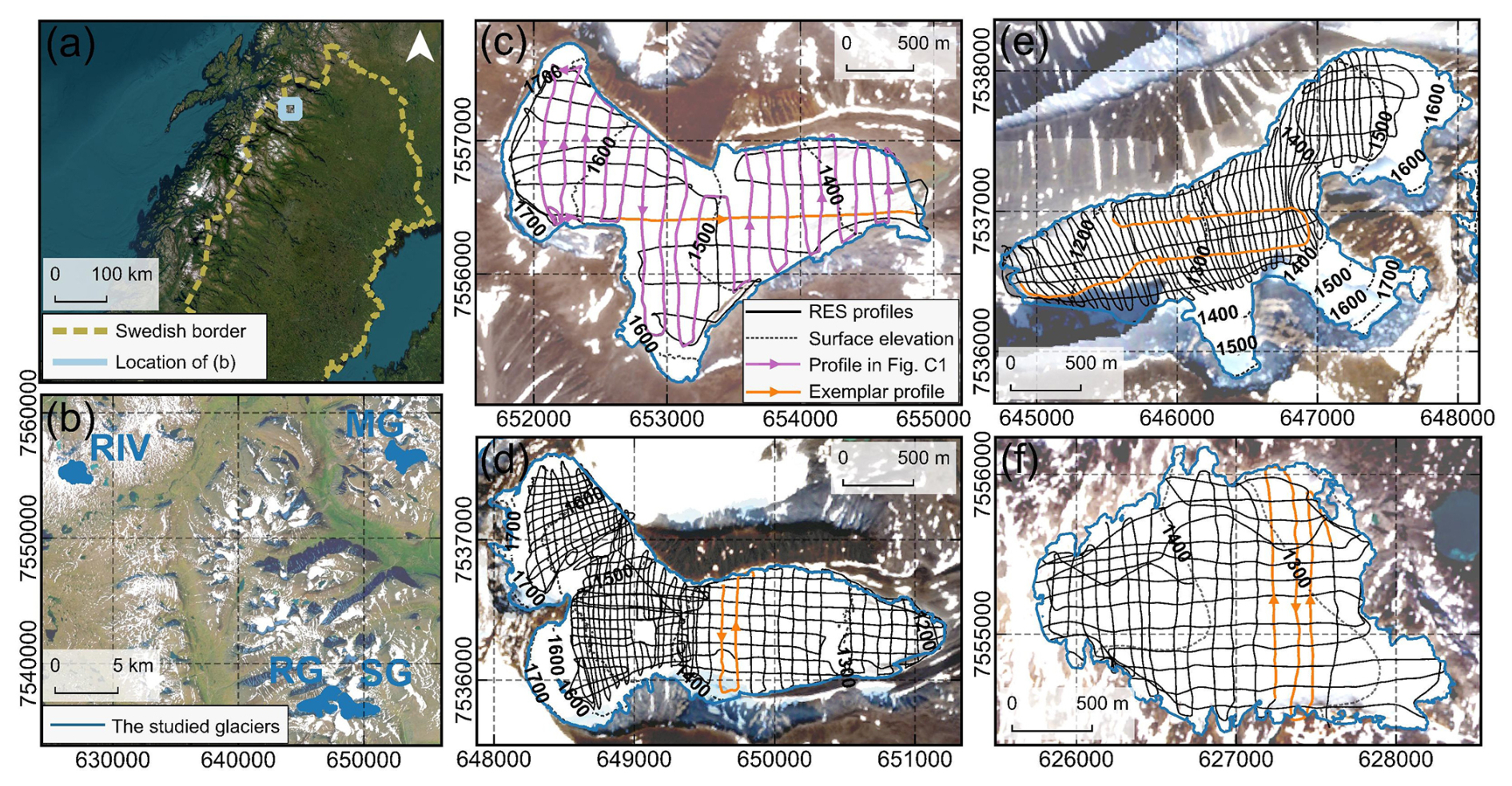
Figure 1 (a) The location of the study area relative to Sweden. The light blue frame shows the location of (b). Background map is from Esri World imagery (Esri, 2025, Powered by Esri). (b) The locations of four reference glaciers MG, SG, RG, and RIV, in the wider Kebnekaise area. Surface elevation (dashed contours, data from Porter et al., 2022) and RES profiles (solid black lines) for (c) MG, (d) SG, (e) RG, and (f) RIV. The dark blue indicate glacier outlines derived from satellite imagery acquired in June 2024. The orange lines represent the exemplar profiles in Fig. 2 as well as Figs. B1–B3 in Appendix B. The purple line highlights the RES profile shown in Fig. C1. Arrows on the RES profiles indicate the survey directions, corresponding to the radargrams from left to right. The maps (b)–(f) use Sentinel-2 L2A imagery acquired on 27 June 2024 (European Space Agency, 2024) as background. Maps were made in QGIS using the SWEREF99 TM coordinate reference system (QGIS Development Team, 2025).

High-resolution ice surface elevations for the four reference glaciers are available from digital elevation models (DEMs), e.g., ArcticDEM (Porter et al., 2022) or Grid2+ (Lantmäteriet, 2019). MG, SG, and RG are all valley glaciers. MG and SG have aspects of 90° (facing east), while RG has an aspect of 270° (facing west). These four glaciers have surface elevation ranges of approximately 1300–1800 m (MG), 1200–1900 m (SG), 1100–1900 m (RG), and 1200–1450 m (RIV) (Porter et al., 2022), with equilibrium line altitudes of 1601 m (MG), 1499 m (SG), 1514 m (RG), and 1380 m (RIV) (WGMS, 2026). MG's accumulation zone is in the northwestern part of the glacier, and ice surface elevations gradually decline eastward towards the glacier's terminus (Fig. 1c). At SG, ice from the two accumulation areas, in the northwest and southwest of the glacier, merge into a comparably flat plateau zone in the centre of the glacier before surface elevations decrease again towards the terminus (Fig. 1d). RG has three accumulation areas in the northeast, southeast, and south. Ice surface elevations decrease from these accumulation areas towards the terminus in the west (Fig. 1e). In contrast to the three aforementioned valley glaciers, RIV is a small ice cap, with surface elevations gradually declining from the west to the east (Fig. 1f). RIV’s subdued surface topography also leads to a mass balance pattern that differs from those of the other three glaciers, i.e., a lower mass balance gradient and the absence of a persistent accumulation zone, whereas the other glaciers generally retain accumulation areas (Tarfala Research Station Staff, 2025a, b, c, d; WGMS, 2026). Over the past 30 years, all four glaciers exhibit cumulative mass losses of approximately −14 to −28 m w.e. (largest for RIV and smallest for SG). Although there is considerable interannual variability, the overall mass balance trend is dominated by increasingly negative summer balances. In contrast, winter accumulation shows relatively small variability and is insufficient to offset enhanced summer melt, indicating sustained glacier thinning and retreat across all sites (Tarfala Research Station Staff, 2025a, b, c, d).

Previous RES surveys were conducted on parts of the reference glaciers to investigate ice thickness and bed topography (Table 1). Bed topography maps are available for SG and RG from 1981 (Björnsson, 1981), and for SG from 1993 (Eriksson, 1993; Herzfeld et al., 1993). However, these maps were hand-contoured based on RES data collected before the introduction of GNSS technology, and therefore involve considerable positioning uncertainty. Due to the unavailability of the previous ice-thickness measurements, the Glacier Thickness Database (GlaThiDa) of the Global Terrestrial Network does not yet include any point thickness measurements for Swedish reference glaciers (GlaThiDa Consortium, 2020; Welty et al., 2020).

Previous modelled ice thickness for the Swedish reference glaciers (Farinotti et al., 2019a; Millan et al., 2022; Frank and van Pelt, 2024) were based on surface observations, i.e., surface elevation, mass balance, and surface velocity of glaciers, while being predominantly calibrated against bed observations of Norwegian glaciers available in the GlaThiDa. The distance to these bed observations and the climatic differences across Scandinavian mountains have introduced considerable uncertainty in the calibration, and consequently, the estimated ice thickness of Swedish glaciers.

Björnsson (1981)Walford et al. (1986)Holmlund (1986)Holmlund and Eriksson (1989)Eriksson (1993)Herzfeld et al. (1993)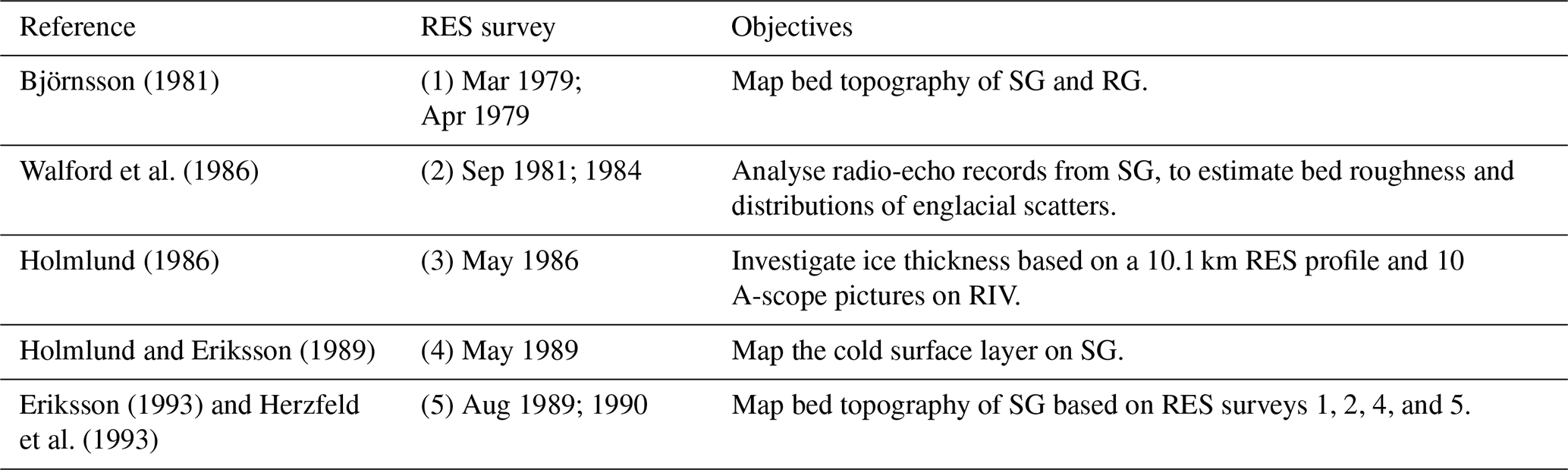

Table 1 Previous RES studies on the four reference glaciers.

3 Methods

3.1 RES data collection

RES surveys were conducted on MG, SG, RG, and RIV during 2024–2025, using a Blue System Integration ice penetrating radar (v3), towed behind a snowmobile (Table 2). This portable impulse radar hardware comprises a 1–200 MHz transmitter, digitizer, computer, and a GPS receiver (Mingo and Flowers, 2010). The GPS receiver is a Garmin OEM18x, with a positioning accuracy of 15 m and an update rate of 5 Hz (Garmin International, Inc., 2024). RES data were collected in an in-line antenna configuration, with antenna separation of 15 m, operating at a central frequency of 10 MHz and a receiver sampling rate of 125 MHz or 250 MHz (Table 2). The snowmobile was driven at a steady speed of 4–6 m s⁻¹. The RES signals were stacked 512 times during acquisition, resulting in a trace spacing of 4–6 m during steady driving.

Table 2 Survey date, sampling rate (“SR”), length of RES surveys (“Length”), survey-line spacing (“Spacing”) along (“AF”) and cross ice flow (“CF”), greatest distance to the nearest known ice-thickness point (“Distance”), percentage of glacier area covered by RES profiles (“Coverage”), and number of RES-measured ice-thickness points after processing (“Points”) for MG, SG, RG, and RIV.

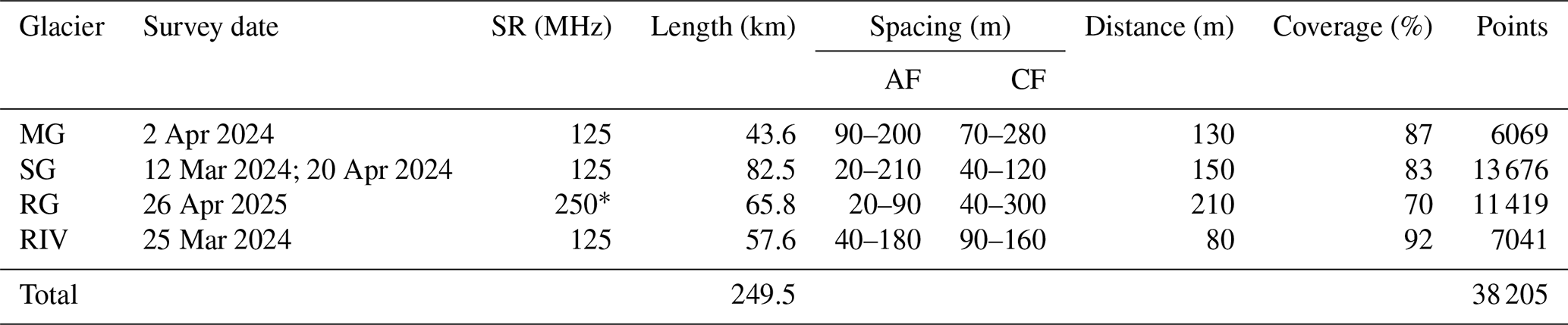
^* A higher sampling rate (250 MHz) was used in the second survey year for RG to improve temporal resolution of RES signal.

RES surveys were conducted at high spatial density, covering most of each glacier's surface. The greatest distance between any location on each glacier and the nearest known ice-thickness point (RES measurements or glacier outline) is within 210 m. Data acquisition was restricted in the upper accumulation zone of SG (near its western boundary) and in the northeastern upper accumulation zone of RG due to steep surface slope and avalanche risk (Fig. 1d, e). Surveys were not carried out in the southern and southeastern parts of RG because of the rockfall risk. RES profiles were planned along a regular grid, however, field conditions (e.g., crevasses and moulins) resulted in some deviations. The grid spacing varies between 20 and 300 m. The survey trajectory was tracked by the GPS receiver integrated into the RES system. The total length of RES surveys is 249.5 km (Table 2).

3.2 RES data processing and interpretation

The subglacial ice-bed interface, i.e., the glacier bed, is a strong electromagnetic reflector because of the dielectric contrast between ice and bedrock or ice and sediment (Dowdeswell and Evans, 2004). As a result, it appears as a distinct reflection in radargrams. In polythermal glaciers, the cold layer has few reflectors or scatterers, making it relatively transparent in radargrams (Pettersson et al., 2003). In contrast, water-filled temperate ice, which is at the pressure melting point, exhibits increased scattering and attenuation due to its different dielectric properties. As a result, it appears opaquer in radargrams, which can lead to ambiguous bed detection (Pettersson et al., 2004; Schannwell et al., 2014) (Fig. 2a). RES data were post-processed using the ReflexW module for 2-D data analysis (Sandmeier, 2024). The data processing workflows for valley glaciers MG (Fig. B1), SG (Fig. 2), and RG (Fig. B2) are designed to enhance bed reflections and include the following steps: dewow, time-zero correction, dynamic correction to account for the 15 m antenna separation, topography correction, signal divergence compensation, 2-D filtering to remove horizontal banding, Butterworth bandpass filtering to retain low-frequency signals (1–5 MHz), and Kirchhoff migration. For RIV, which contains relatively shallow ice, a simplified processing flow comprising time-zero correction, dynamic correction, topography correction, 2-D filtering, and Kirchhoff migration was applied (Fig. B3). The radargrams (Figs. 2, B1–B3) were rescaled using GPS-recorded positions to account for variable trace spacing caused by changes in acquisition speed, ensuring that the horizontal axis represents true distance.

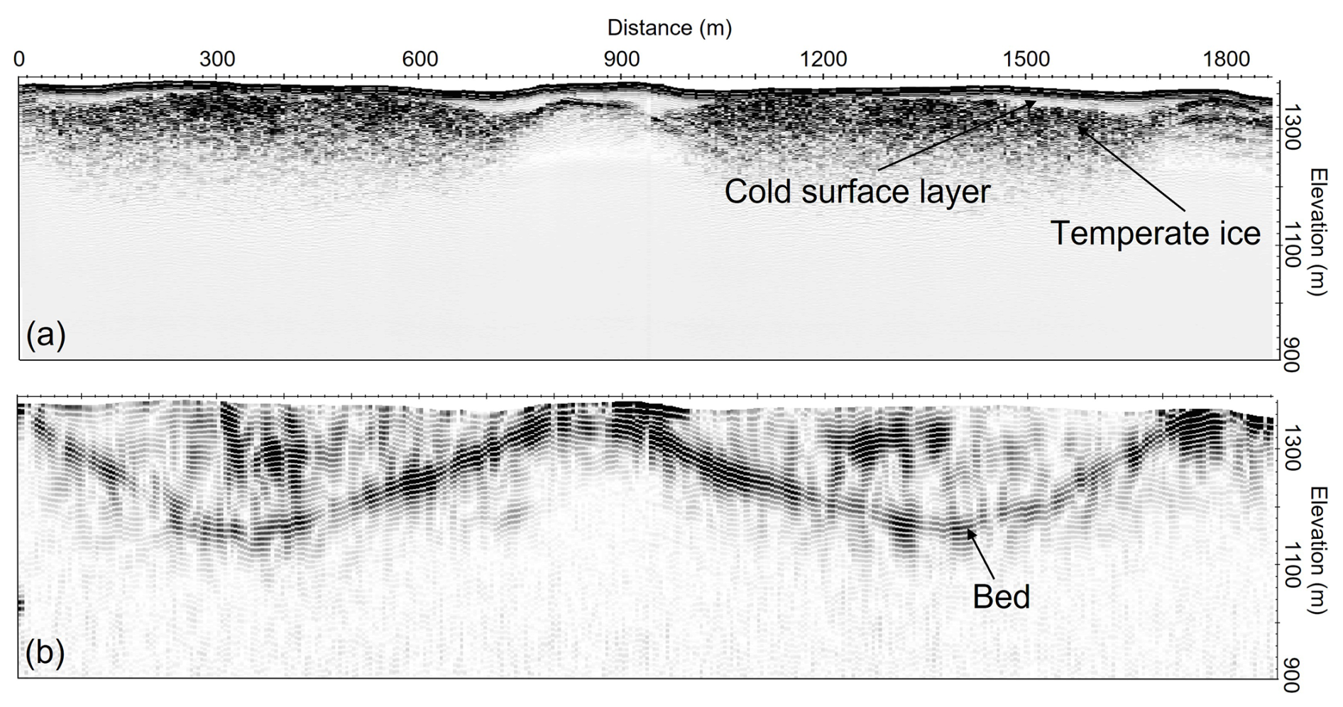
Figure 2 Exemplar RES profile MAR122410H1918 on SG (orange profile in Fig. 1d): (a) RES data after only time-zero correction and topography correction, displaying englacial scattering from temperate ice, and (b) fully processed RES data revealing the glacier bed and the suppression of englacial scattering.

For polythermal glaciers, the glacier bed is generally picked manually from radargrams (Grab et al., 2021), as strong signal scattering in the temperate ice can complicate automatic or semi-automatic bed identifications (e.g. Fig. 2a). However, manual picking is time-consuming and prone to subjective bias. Therefore, here we combined both automatic and manual approaches for bed identification, to achieve a balance between efficiency, objectivity, and accuracy. The preliminary glacier bed picks, expressed in units of two-way travel time (TWT), were obtained automatically through batch analysis in ReflexW and MATLAB (The MathWorks Inc., 2024) following this workflow: (a) the Hilbert transform was applied to generate the signal envelope of the fully processed data using trace analysis in ReflexW. The resulting envelope data were then imported into MATLAB; (b) the maximum reflection was identified in each trace and interpreted as the bed; (c) static traces (where GPS trace spacing <1 m) were removed; (d) adjacent bed picks with large TWT difference were taken as potential erroneous picks and removed; and (e) outlier picks were further filtered using a move median filter, thereby removing surface maximum picks (likely caused by crevasses) as well as other unreliable picks (Fig. C1a). The automatic preliminary bed picks were used to evaluate the data quality and rapidly generate preliminary ice thickness and bed topography maps. The preliminary automatic bed picks were then imported into ReflexW for further manual refinement, where misidentified bed picks were repicked. For manual repicking, the bed reflections were first traced on radargrams that were not bandpass filtered, where the bed reflections not covered by temperate ice were clearly visible. Subsequently, filtered radargrams retaining only the low-frequency components were used in areas where the bed reflections were ambiguous or not visible in the unfiltered radargrams. This process allows bed identification while minimizing inaccurate interface tracking caused by filter-induced pulse broadening. In addition, weak bed reflections caused by steeply dipping reflectors or reflectors at great depth, and multiple basal reflectors were unpicked to improve the accuracy of the overall data interpretation (Fig. C1b).

We calculated point ice thickness (H) from the TWT of bed picks (t) using a constant radio-wave velocity of 168 m µs⁻¹ in ice (v), the same value was used previously for SG (Pettersson et al., 2003) and other glaciers (Dowdeswell and Evans, 2004; Gillespie et al., 2024):

$$\begin{array}{}\text{(1)}& H={\displaystyle \frac{tv}{\mathrm{2}}}.\end{array}$$

3.3 Uncertainty analysis of RES-measured ice thickness

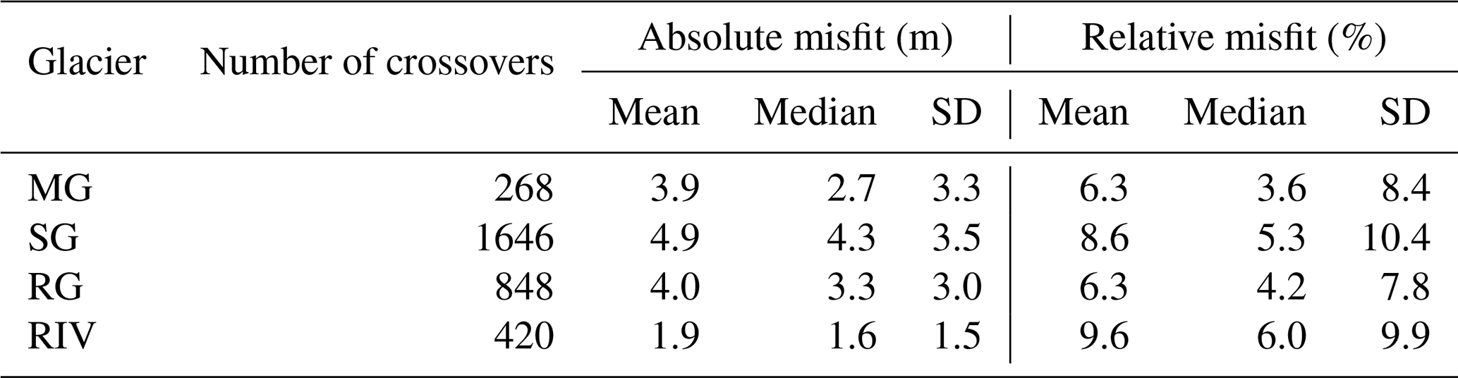
We assessed the within RES dataset consistency by comparing ice thicknesses at intersection points, i.e., crossovers between survey lines. RES data points from different survey directions less than 5 m apart (the average trace spacing) were considered as crossovers. Ice thicknesses at crossovers exhibit small absolute misfits but larger relative misfit for RIV and near glacier boundaries, primarily affected by the relatively shallow ice in these areas (Table 3). Crossover analysis shows some significant inconsistencies along or near valley walls, and during sharp turns. We accordingly unpicked those bed reflectors to limit the influence of out-of-plane reflections and incomplete extension of the antennas. In total, 38 205 point values of RES-measured ice thickness were presented for the four reference glaciers (Table 2).

Table 3 Data statistics for MG, SG, RG, and RIV, including number of crossovers, as well as mean, median, and standard deviation of absolute and relative crossover misfits. The number of crossovers refers to pairs of RES data points from different survey directions located within 5 m of each other.

Whilst crossover analysis can reveal inaccurate bed picks by comparing discrepancies between RES measurements, it does not quantify ice-thickness uncertainty for each RES data point. We therefore calculated the uncertainty using standard analytical error propagation methods (Lapazaran et al., 2016). The total uncertainty ϵ_H includes contributions from RES measurement uncertainty ${\mathit{ϵ}}_{H_{\text{RES}}}$ and from uncertainty in the positioning of data points ${\mathit{ϵ}}_{H_{xy}}$:

$$\begin{array}{}\text{(2)}& {\mathit{ϵ}}_H=\sqrt{{\mathit{ϵ}}_{H_{\text{RES}}}^{\mathrm{2}}+{\mathit{ϵ}}_{H_{xy}}^{\mathrm{2}}}.\end{array}$$

Applying error propagation to Eq. (1), RES measurement uncertainty ${\mathit{ϵ}}_{H_{\text{RES}}}$ is a function of radio-wave velocity v, TWT t, their errors ϵ_v and ϵ_t:

$$\begin{array}{}\text{(3)}& {\mathit{ϵ}}_{H_{\text{RES}}}={\displaystyle \frac{\mathrm{1}}{\mathrm{2}}}\sqrt{v^{\mathrm{2}}{\mathit{ϵ}}_t^{\mathrm{2}}+t^{\mathrm{2}}{\mathit{ϵ}}_v^{\mathrm{2}}}.\end{array}$$

Note that radio-wave velocity v varies spatially, as it is influenced by the density and water/air content of snow, firn, and cold/temperate ice layers. Assuming a constant v for all RES data points (168 m µs⁻¹) can result in biased ice thickness estimates, e.g. overestimations in the ablation zone and underestimations in the accumulation zone. Lapazaran et al. (2016) proposed that uncertainties in v vary from ∼1 % to ∼5 %, for polythermal glaciers. In our study, we used 5 m µs⁻¹ as ϵ_v following Grab et al. (2021). We used range resolution of the RES data as ϵ_t, which represents how precisely the reflections can be identified. Range resolution is generally evaluated between one-quarter and half the RES wavelength, corresponding to 4.2–8.4 m for our unprocessed dataset. Considering the additional uncertainties introduced by data processing and manual interpretation, ϵ_t values of 80, 150, and 250 ns (representing 6.7, 12.6, and 21 m in the ice) were assigned to bed reflections of varying identification quality.

We estimated the positioning-related ice-thickness uncertainty ${\mathit{ϵ}}_{H_{xy}}$, as the maximum discrepancy in ice thickness between a RES data point and its adjacent points located within ϵ_xy, which represents the positioning uncertainty:

$$\begin{array}{}\text{(4)}& {\mathit{ϵ}}_{xy}=\sqrt{{\mathit{ϵ}}_{xy\text{GPS}}^{\mathrm{2}}+{\mathit{ϵ}}_{\mathrm{\Delta }xy}^{\mathrm{2}}},\end{array}$$

ϵ_xy has two components, ϵ_xyGPS is horizontal positioning accuracy of the GPS, and ϵ_Δxy represents the displacement of the RES system occurring within the time lag between the GPS coordinate update and the trace recording (ϵ_T):

$$\begin{array}{}\text{(5)}& {\mathit{ϵ}}_{\mathrm{\Delta }xy}=v_{\text{RES}}{\mathit{ϵ}}_{\mathrm{T}},\end{array}$$

where v_RES is the travel speed of the RES system, which in our case equals the snowmobile driving speed of 5 m s⁻¹. ϵ_T is estimated as the GPS update period.

3.4 Model-based ice thickness distribution, uncertainty, and bed topography

Due to the ground-based nature of the surveys, RES profiles could not be conducted over areas with moulins, large crevasses, and steep ice surface slopes. We interpolated and extrapolated RES-measured ice thickness to obtain continuous ice thickness distribution (hereafter referred to as “distributed ice thickness” to distinguish them from RES-measured ice thickness) using a model-based approach. Based on Farinotti et al. (2017, 2021) who compared the performance of different ice thickness models, we selected the Glacier Thickness Estimation algorithm (GlaTE) (Langhammer et al., 2019), which performs well where observation data coverage is relatively high. GlaTE is based on mass conservation, apparent mass balances, and Glen's ice flow law. It considers both constraints from RES data and glaciological modelling in inversion.

We input glacier surface elevation, glacier outlines, as well as RES-measured ice thicknesses and their associated uncertainties to GlaTE. ArcticDEM strips acquired closest in time to the RES data acquisition were used as surface elevations. They were acquired in 1 October 2022 (MG), 5 October 2024 (SG), 5 October 2024 (RG), and 17 May 2024 (RIV), respectively, thus ranging from more than 1.5 years before (MG) to a few weeks after (RIV) RES data acquisition in the field. For MG, RG, and RIV, the ArcticDEM elevations were corrected using vertical offsets of −1.7, 2.5, and −0.1 m based on dGNSS point elevations (Table D1) measured in 2 April 2024 (MG), 21 April 2025 (RG), and 25 March 2024 (RIV), respectively (the dates closest to the RES data acquisition). The −1.7 m adjustment for MG represents cumulative surface elevation changes during the period autumn 2022 to spring 2024, whereas the 2.5 m adjustment for RG captures substantial snow accumulation during the winter 2024/2025. The relatively small correction value for RIV is explained by the temporal proximity of the ArcticDEM strip and the RES survey. The ArcticDEM elevation was not corrected for SG because of the lack of dGNSS measurements in 2024. Latest glacier outlines identified from 2024 Sentinel-2 imagery were selected as input for the model, and used to adjust ice thickness at the glacier boundary to zero. RES-measured ice thicknesses and their uncertainties were used to constrain the modelled ice thickness in GlaTE. In the model, we assigned apparent mass balance gradients for the accumulation/ablation zones of MG, SG, RG, and RIV as $\mathrm{0.0056}/\mathrm{0.0069}$, $\mathrm{0.0045}/\mathrm{0.0067}$, $\mathrm{0.0053}/\mathrm{0.0063}$, and $\mathrm{0.00054}/\mathrm{0.00098}$ m w.e. m⁻¹ yr⁻¹, respectively, based on mass balance surveys conducted over the most recent three years (WGMS, 2026). We finally obtained distributed ice thickness maps for four reference glaciers with a spatial resolution of 10 × 10 m. It should be noted that this does not represent the realistic spatial resolution away from the RES survey lines. This is because GlaTE relies on surface information, which physically limits the spatial detail that can be resolved in the modelled bed, i.e. bed features smaller than at least one ice thickness cannot be recovered (Raymond and Gudmundsson, 2005; Gudmundsson and Raymond, 2008).

We repeated the modelling using the maximum and minimum RES-measured ice thickness within the ϵ_H range, the absolute difference between distributed ice thickness was taken as the uncertainty of distributed ice thickness. This estimate represents a lower bound of the true uncertainty, as it does not include uncertainty contributions from the interpolation method and from the surface elevation dataset used. The interpolation uncertainty is related to multiple mechanical and smoothing parameters, while the surface elevation uncertainty depends on data resolution and acquisition time, both of which are difficult to quantify explicitly. The misfit between the distributed ice thickness and RES-measured ice thickness was calculated along RES survey lines.

Bed topography was calculated by subtracting distributed ice thickness datasets from the calibrated surface elevation for each glacier. Our final bed topography products were smoothed using a Gaussian filter with a spatial smoothing scale of approximately 60 m and calibrated to the geoid using geoid model SWEN17_RH2000 (Lantmäteriet, 2017).

4 Data description and evaluation

4.1 RES-measured ice thickness and uncertainty

The RES-measured ice thicknesses were compiled in a similar format as “Table TTT. Glacier thickness: Point measurements” in GlaThiDa (Welty et al., 2020; Gillespie et al., 2024) to ensure the data accessibility and reusability (Wang et al., 2026a, b, c, d). The along track ice thickness data are provided in a CSV (comma-separated values) table containing the following fields: glacier name (GLACIER_NAME), survey date (SURVEY_DATE), RES profile identifier (PROFILE_NAME), RES point identifier (POINT_ID), latitude and longitude of each RES point (POINT_LAT and POINT_LON), calibrated surface elevation (ELEVATION), ice thickness (THICKNESS), and corresponding ice-thickness uncertainty (UNCERTAINTY).

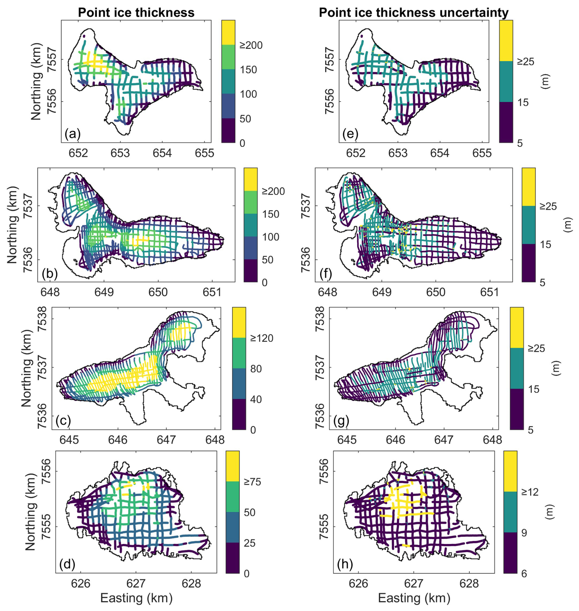
Figure 3 Point RES-measured ice thickness (a–d) and total ice-thickness uncertainty (e–h) for MG, SG, RG, and RIV, respectively.

For MG, thickest ice (241 m) is located in the northwestern part. The southern section of the glacier also has relatively thick ice (Fig. 3a). For SG, the thickest ice is found in the central section, where the glacier narrows and then widens into the central plateau region, reaching a maximum of 225 m. In the western accumulation zone there is relatively thick ice of ∼200 m (Fig. 3b). For RG, the maximum measured ice-thickness is 158 m in the centre of the glacier after ice converges from the northeastern and southeastern accumulation areas. The northeastern part has relatively thick ice of ∼150 m (Fig. 3c). For RIV, the maximum measured ice thickness is 88 m in the northern part of the glacier. Relatively thick ice on RIV is found in its middle-north section (Fig. 3d). Overall, MG is the thickest among the four reference glaciers, followed by SG and RG, while RIV is relatively shallow compared with the other three glaciers (Table 4).

Larger ice-thickness uncertainty related to RES measurement (${\mathit{ϵ}}_{H_{\text{RES}}}$) are found where the ice is thicker or the bed is harder to identify in radargrams (Fig. E1a–d). In contrast, ice-thickness uncertainty related to positioning error (${\mathit{ϵ}}_{H_{xy}}$) shows a relatively uniform distribution, with larger values in areas of steeper slopes (Fig. E1e–h). Overall, the total ice-thickness uncertainties (ϵ_H) are primarily related to ${\mathit{ϵ}}_{H_{\text{RES}}}$ (Fig. 3e–h). Compared with the other three glaciers, RIV has substantially smaller ice thickness and ice-thickness uncertainty (Table 4).

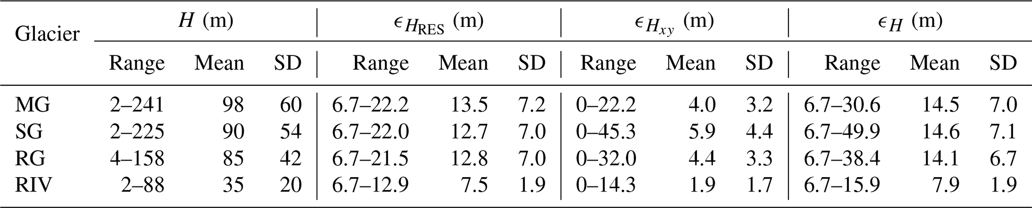
Table 4 Range, mean, and standard deviation of RES-measured ice thicknesses and ice-thickness uncertainties for MG, SG, RG, RIV.

4.2 Distributed ice thickness, uncertainty, and ice volume

Distributed ice thickness maps exhibit the continuous ice thickness variations over each glacier (Fig. 4a, d, g, j). By integrating the ice thickness over the glacier area, we obtained ice volume estimates of 0.32 (MG), 0.25 (SG), 0.23 (RG), and 0.10 km³ (RIV), respectively.

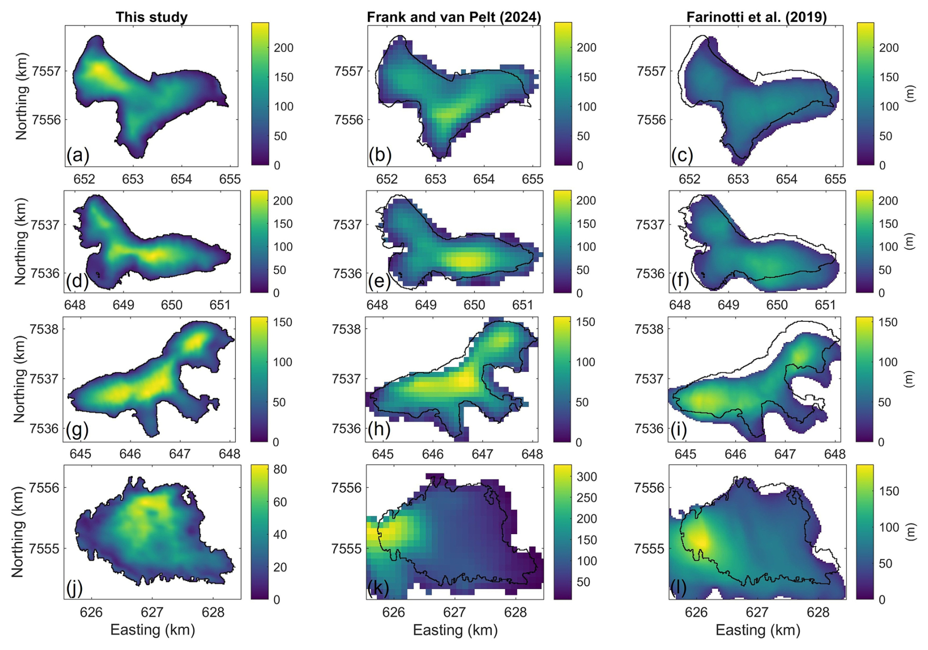
Figure 4 Distributed ice thickness from this study, as well as previous modelled ice thickness from Frank and van Pelt (2024) and Farinotti et al. (2019a) for MG (a–c), SG (d–f), RG (g–i), and RIV (j–l).

Consistent with RES observations, MG contains the thickest ice (∼ 240 m) among four reference glaciers (Table 5). MG, SG, and RG exhibit different ice-thickness patterns. The thickest ice at MG is within its accumulation zone, whereas SG and RG have the thickest ice in the central sectors, where ice converges from different accumulation areas. The thicker ice at RG extends to the lower ablation area. The differences between the glacier ice thicknesses is likely related to the glacier geometries (Fig. 1c–d) and bed topography. At RIV, the thickest ice (∼ 80 m) displays a saddle-shaped pattern in the northern sector, which is consistent with earlier observations by Holmlund (1986). The ∼ 20 m difference between our maximum ice thickness and the previous estimates can be explained by mass loss over the past 28 years.

The mean uncertainties of distributed ice thickness are 27.0 (MG), 24.7 (SG), 21.3 (RG), and 12.9 m (RIV) for the four glaciers (Fig. 5a–d). Overall, larger distributed uncertainties concentrate in the thicker, interior regions of the glaciers. Misfits between distributed ice thickness and RES-measured ice thickness are larger near the ice margins, where the model assumes zero ice thickness based on the glacier outlines. This occasionally contradicts the RES measurements, primarily due to temporal asynchrony between the RES surveys and the satellite images from which the glacier outlines were extracted (Fig. 5e–h).

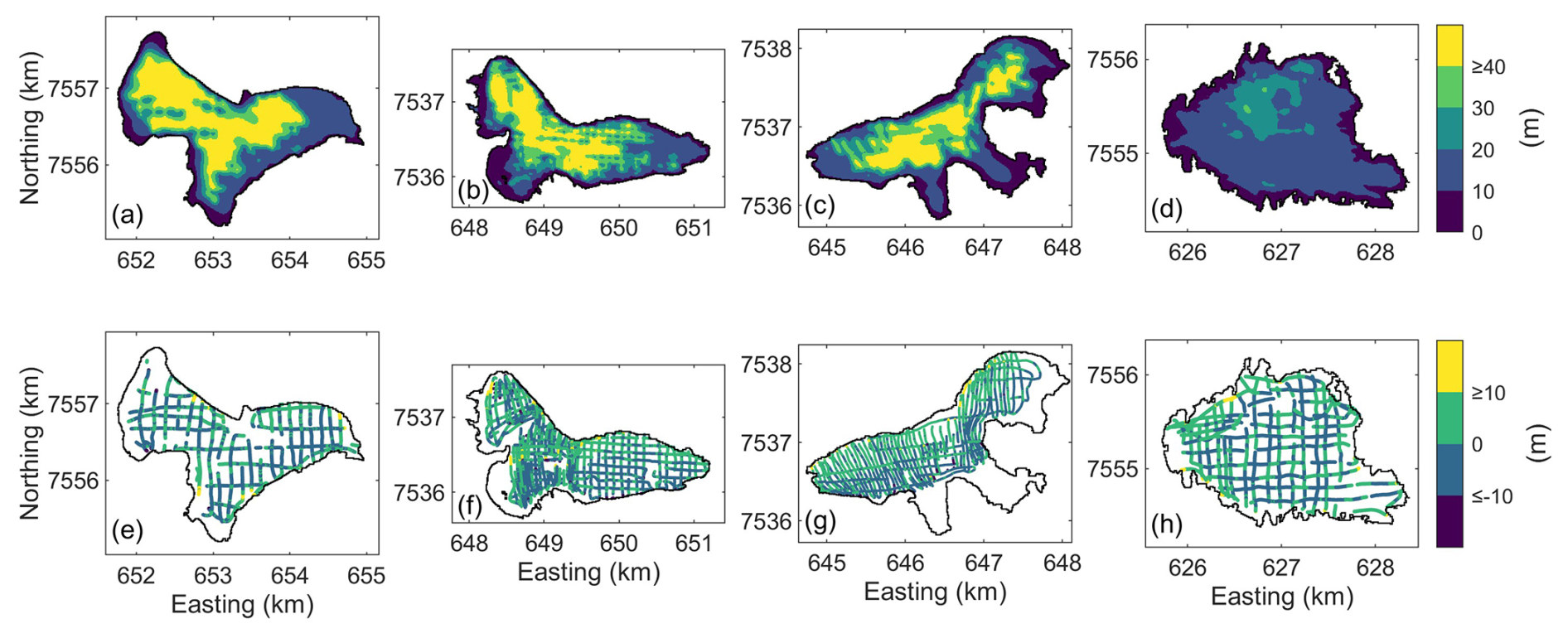
Figure 5 The uncertainty of distributed ice thickness for (a) MG, (b) SG, (c) RG, and (d) RIV. The misfit between distributed ice thickness and point RES-measured ice thickness for (e) MG, (f) SG, (g) RG, and (h) RIV.

We compared our distributed ice thickness of four Swedish reference glaciers with those from previous studies (Fig. 4, Table 5). Frank and van Pelt (2024) estimated the ice thickness of Scandinavian glaciers using the Instructed Glacier Model (Jouvet and Cordonnier, 2023), which is based on a higher-order ice flow approximation. Their approaches (Frank et al., 2023) incorporated surface elevation (Lantmäteriet, 2019) and its rate of change (Hugonnet et al., 2021), mass balance (Rounce et al., 2023), and glacier outlines corrected by them from RGI 6.0 (RGI Consortium, 2017) to address systematic misalignment with topography. Additionally, previous bed elevation for SG (Björnsson, 1981) was used for ice-thickness calibration. The mean absolute ice-thickness misfits between their study and ours are 36, 31, 21, and 72 m for MG, SG, RG, and RIV, respectively (Fig. 4b, e, h, k). Farinotti et al. (2019a) provided a consensus estimate of global ice thickness using an ensemble of up to five models considering surface characteristics. Their estimates were based on RGI 6.0 and thus exhibit misaligned glacier outlines (Fig. 4c, f, i, l). Millan et al. (2022) estimated global ice volumes and ice thicknesses based on high-resolution mapping of ice motion during the period 2017–2018, using glacier outlines from the RGI 6.0. Compared with our results and the other two modelled estimates, these ice thicknesses (Millan et al., 2022) are clearly overestimated. This discrepancy is likely related to the model's strong dependence on surface flow velocity, which is relatively low (0–18 m yr⁻¹ in 2022 reported by Gardner et al., 2024) and thus difficult to constrain accurately for the four Swedish reference glaciers (Table 5). Therefore, we do not include this study in further comparative analyses.

Table 5 Comparison of mean distributed ice thicknesses and ice volumes of MG, SG, RG, and RIV obtained in this study and previous studies.

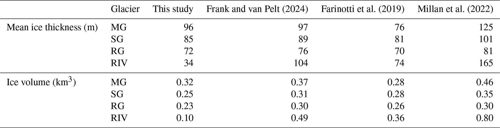
Previous studies for the four reference glaciers (Farinotti et al., 2019a; Frank and van Pelt, 2024) are based on observational input data obtained in the past, e.g., glacier outlines obtained around 2001–2002 (GLIMS Consortium, 2005). Thus their ice-thickness estimates correspond to an earlier time period than ours. Given the observed ice losses in the recent years, which are quantified as 0.030 (MG), 0.019 (SG), 0.029 (RG), and 0.026 km³ (RIV) during 2017–2024 based on continuous annual mass balance records (Tarfala Research Station Staff, 2025a, b, c, d) and glacier area records (Table A1), the previous studies should show larger ice volumes and ice thicknesses relative to this study. However, Farinotti et al. (2019a) presented smaller mean ice thicknesses for MG, SG, and RG, indicating an underestimation of their results. Frank and van Pelt (2024) reported larger ice volumes and mean ice thicknesses for SG, MG, and RG than our study, which are likely related to glacier mass and area losses between their research period and ours. Frank and van Pelt (2024) suggested that their estimates correspond approximately to the year 2010. Assuming similar mass loss rates during 2010–2017 as observed for 2017–2024, their results would slightly underestimate ice volume for MG by ∼  2.7 %, while overestimating ice volume for SG and RG by ∼ 7.1 % and ∼ 4 %, respectively. For RIV, both Frank and van Pelt (2024) and Farinotti et al. (2019a) significantly overestimated ice thickness and ice volume as they both relied on the RGI 6.0 glacier outline. This outline corresponds to approximately twice the current RIV area (Fig. 4j–l), directly affecting the ice volume calculation. Moreover, ice-free terrain included within the overly large outline violates a key requirement for meaningful ice thickness inversions, which generally rely on a glacier mask to define the modelling domain. As a result, the modelled thicknesses in such areas are unreliable.

There are also notable differences in spatial ice-thickness distributions between previous studies and our work (Fig. 4). For MG, our RES measurements indicate the thickest ice in the northwest, whereas Frank and van Pelt (2024) and Farinotti et al. (2019a) both reported thicker ice in the south and in the central section while both underestimated ice thickness in the northwestern part (Fig. 4b–c). This underestimation may result from inaccuracies in the mass balance data used in the modelling, as both Frank and van Pelt (2024) and Farinotti et al. (2019a) rely on elevation-dependent gradients, but could also arise from assumptions regarding sliding and ice viscosity, surface elevation data input, or incomplete representation of ice flow physics. For SG, both Frank and van Pelt (2024) and Farinotti et al. (2019a) derived the thickest ice in the central glacier (Fig. 4e–f). Similar to our results, Farinotti et al. (2019a) also obtained relatively thick ice in the northwestern part of glacier, while Frank and van Pelt (2024) underestimated the ice thickness there. For RG, Frank and van Pelt (2024) and Farinotti et al. (2019a) showed ice-thickness patterns broadly consistent with our results, i.e. thick ice in the central and northeastern glacier (Fig. 4h–i). Frank and van Pelt (2024) underestimated the ice thickness near to the glacier terminus. For RIV, the ice-thickness distributions from Frank and van Pelt (2024) and Farinotti et al. (2019a) do not agree with our result (Fig. 4k–l), primarily due to inaccurate glacier outlines. Overall, Frank and van Pelt (2024) and Farinotti et al. (2019a) captured the broad patterns of the ice-thickness distribution for MG, SG, and RG. However, Frank and van Pelt (2024) tended to underestimate ice thickness in accumulation zones, whereas Farinotti et al. (2019a) systematically underestimated ice thickness across the glaciers. Although these global and regional studies often rely on coarser data, trading spatial resolution for broader coverage, this comparison still highlights the importance of RES measurements for accurately mapping ice-thickness distributions, both for Swedish glaciers and for other glaciers across the world.

4.3 Bed topography

At MG, the subglacial topography reveals a depression in the eastern part of the glacier, with the lowest elevation ∼ 1300 m above sea level (a.s.l., referenced to the geoid model SWEN17_RH2000). The bed gradually rises towards the glacier boundary surrounding this depression, reaching elevations up to ∼ 1800 m a.s.l. along the northwestern and southern margin (Fig. 6a). At SG, an elongated trough is situated in the central-eastern part, containing two depressions at ∼ 1150 m a.s.l. The bed elevation increases towards the glacier boundary in the southwest, reaching a maximum of ∼ 1700 m a.s.l. In the northwestern part, there is a depression with an elevation of ∼ 1400 m a.s.l., before the bed rises to ∼ 1900 m.a.s.l. in the uppermost accumulation zone (Fig. 6b). At RG, there is a pronounced deepening along the central section and towards the glacier terminus, where the bed elevation reaches a minimum of ∼ 1100 m a.s.l. The bed rises towards the three accumulation areas of RG, approaching a maximum elevation of ∼ 1900 m a.s.l. near the southeastern glacier boundary (Fig. 6c). Each of these three glaciers is associated with a trough along its central section, through which ice flows. Unlike the three valley glaciers, the glacier bed at RIV does not vary substantially in elevation. Instead, the bed gradually descends from a maximum elevation of ∼ 1430 m a.s.l. in the west to a minimum elevation of ∼ 1200 m a.s.l. in the east (Fig. 6d).

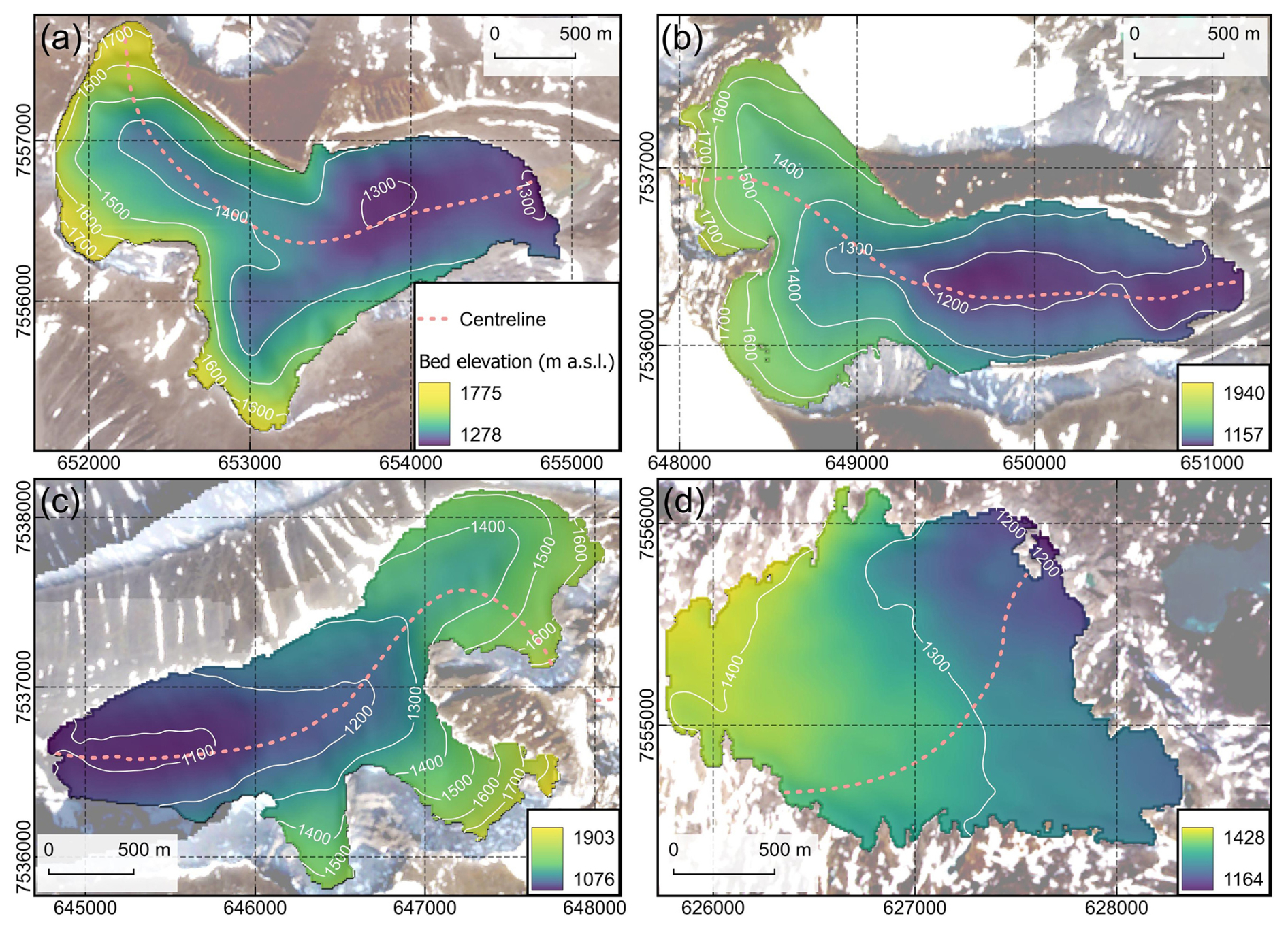
Figure 6 Bed topography of (a) MG, (b) SG, (c) RG, and (d) RIV. White lines represent the contours of bed elevation. Pink dashed lines represent the glacier branch centrelines defined in RGI7.0 (RGI Consortium, 2023) and the locations of topographic profiles in Fig. 7. The maps use Sentinel-2 L2A imagery (European Space Agency, 2024) as background.

To visualize the topographic variations, we have plotted the bed elevation and surface elevation of selected profiles for four reference glaciers (Fig. 7). In MG (Fig. 7a), a small depression in bed topography in the northwestern section (500–1200 m) corresponds to locally thicker ice in the upper glacier. In contrast, SG (Fig. 7b) and RG (Fig. 7c) show a more continuously descending bed, which is associated with thicker ice along the central flowline, extending towards the central and lower parts of the glaciers. The bed descends by only ∼ 120 m along the centreline across RIV, it shows no clear relationship with ice thickness (Fig. 7d).

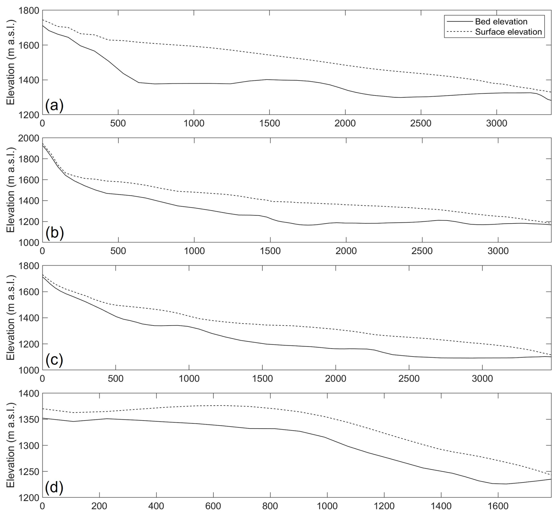
Figure 7 The bed elevation (solid line) and surface elevation (dashed line) of selected profiles for (a) MG, (b) SG, (c) RG, and (d) RIV, along their branch centrelines (pink lines in Fig. 6). The profiles are oriented from left to right in the direction of decreasing bed elevation.

Our results and previous RES-derived bed topography of SG (Herzfeld et al., 1993) and RG (Björnsson, 1981) show good consistency in both values and patterns (Fig. 8). Both our and previous maps of SG reveal two depressions in the central-eastern section with an elevation of ∼ 1150 m a.s.l., as well as a smaller depression at ∼ 1400–1450 m in the northwestern part. Both maps of RG reveal the deepening along the central section towards the terminus. With denser and more modern RES measurements, our high-resolution maps reveal small-scale undulations of bed topography. Moreover, our digital maps enable reusability in the future.

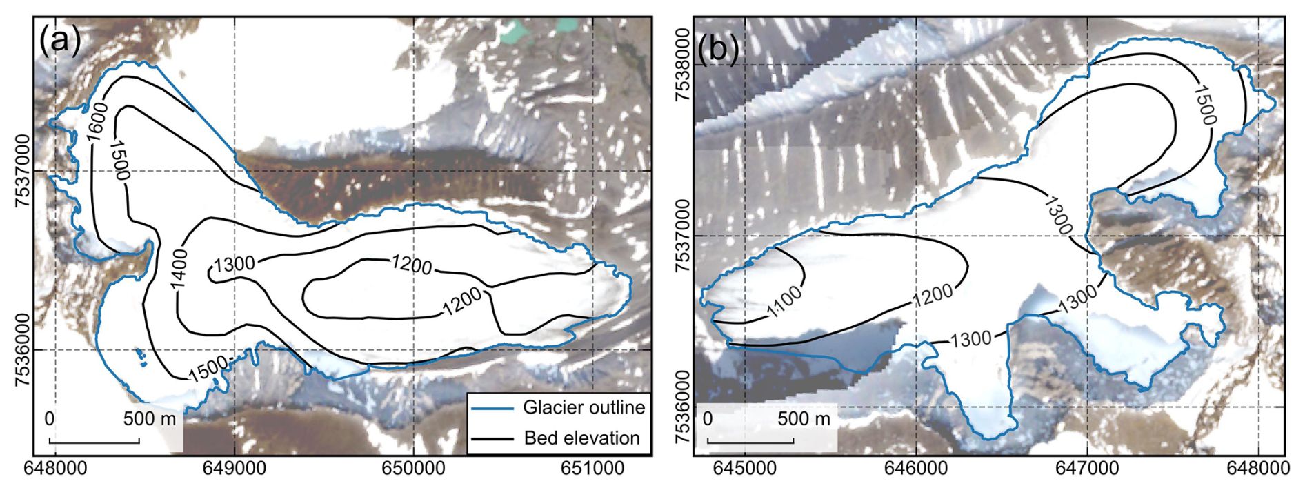
Figure 8 Previous hand-contoured maps of (a) SG bed topography (Herzfeld et al., 1993) and (b) RG bed topography (Björnsson, 1981). The maps use Sentinel-2 L2A imagery (European Space Agency, 2024) as background. The maps are georeferenced and digitized in QGIS (QGIS Development Team, 2025), with unavoidable errors.

4.4 Potential applications for the data

Currently, no point measurements of ice thickness from Swedish glaciers are included in the global ice-thickness database GlaThiDa (GlaThiDa Consortium, 2020), our datasets fill this gap and have considerable value across a wide range of disciplines.

The newly obtained ice thickness measurements can contribute to improving ice-thickness modelling for Swedish glaciers by constraining modelling parameters (such as ice viscosity). For example, we calibrated global model parameters using RES-measured ice thicknesses and repeated the experiment described in Frank and van Pelt (2024) for MG. The model estimates more accurate ice thickness in the northwestern and central section (Fig. F1). The mean absolute misfit between the updated modelled ice thickness and our result is 31 m, representing a 20 % reduction compared with their original modelled misfit.

Our bed topography maps provide essential boundary conditions for numerical modelling. They can be used for future studies of glacier evolution to improve projections of the remaining lifetimes of these glaciers (Rounce et al., 2023; Zekollari et al., 2025). They can also support simulations of future hydrological changes within glacier catchments of four reference glaciers, e.g., determining water routing and locating future glacier lakes (Otto et al., 2022; Steffen et al., 2022).

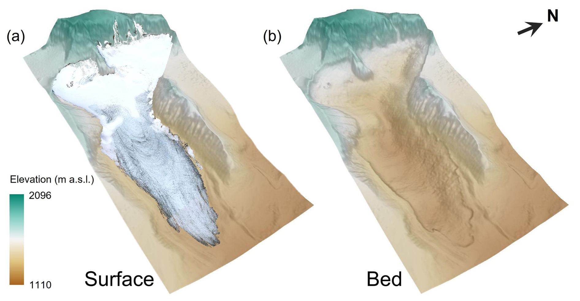
Figure 9 3D topography of (a) the glacier surface and (b) the bed of SG, illustrating the present-day landscape and the projected post-glacial landscape, respectively.

Annual ice volumes of the four reference glaciers can be quantified by combining our bed topography maps with annual high-resolution surface DEMs, which can be acquired using uncrewed aerial vehicles. Furthermore, bed topography maps reveal characteristics of the landscapes that will be exposed during the future post-glacial time (Fig. 9). They provide insights into the potential geohazards (e.g. landslides, debris flows, and rockfalls) which might occur as landscape stability changes during glacier retreat.

The above predictions are crucial for local policymaking during glacier retreat and in the post-glacial future, when formerly glacier-covered areas become ice-free. This is particularly relevant for tourism planning, infrastructure development, and the sustainable livelihoods of Indigenous communities who rely on natural environments (Carey, 2010; Welling et al., 2015).

5 Data availability

All datasets are available through the Bolin Centre Database (Table 6).

(Wang et al., 2026f)(Wang et al., 2026h)(Wang et al., 2026e)(Wang et al., 2026g)(Wang et al., 2026a)(Wang et al., 2026d)(Wang et al., 2026b)(Wang et al., 2026c)

Table 6 Datasets and their corresponding DOIs.

6 Code availability

The code is available at https://doi.org/10.5281/zenodo.18001737 (Wang, 2026).

7 Conclusions

In this study, we compile 38205 ice thickness point measurements collected by RES during 2024–2025 for four Swedish reference glaciers, i.e. MG, SG, RG, and RIV. The mean measured ice thicknesses are 98 ± 14.5, 90 ± 14.6, 85 ± 14.1, and 35 ± 7.9 m for MG, SG, RG, and RIV, respectively. The corresponding maximum measured ice thicknesses are 241, 225, 158, and 88 m. Based on these datasets, we produce maps of distributed ice thickness and bed topography with a spatial resolution of 10 × 10 m. The mean distributed ice thicknesses are 96 ± 27.0 (MG), 85 ± 24.7 (SG), 72 ± 21.3 (RG), and 34 ± 12.9 m (RIV), respectively. The corresponding ice volumes are 0.32, 0.25, 0.23, and 0.10 km³. Our results provide up-to-date ice thickness distribution based on observations. Additionally, we present digital bed topography maps for the four Swedish reference glaciers for the first time. The compiled datasets and derived maps are valuable for future studies on glacier dynamics, and for projecting the evolution of glaciers, landscapes, ecology, and hydrology in the Arctic mountain environments of northern Scandinavia.

Appendix A

Table A1 Records of mass balance (Tarfala Research Station Staff, 2025a, b, c, d) and glacier area during period 2017–2024 (Houssais et al., 2025) for MG, SG, RG, and RIV, respectively.

Appendix B

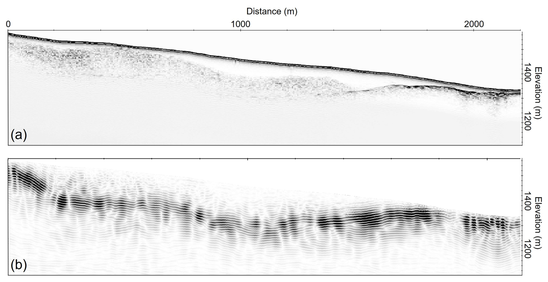
Figure B1 Exemplar RES section (part of profile APRIL2FILE1N) on MG (orange line in Fig. 1c): (a) RES data after time-zero correction and topography correction only, and (b) fully processed RES data revealing the glacier bed.

Figure B2 Exemplar RES section (part of profile Apr262511H5602) on RG (orange line in Fig. 1e): (a) RES data after time-zero correction and topography correction only, and (b) fully processed RES data revealing the glacier bed.

Figure B3 Exemplar RES section (part of profile Mar252411H0212) on RIV (orange line in Fig. 1f): (a) RES data after time-zero correction and topography correction only, and (b) fully processed RES data.

Appendix C

Figure C1 For RES profile APR022414H4605 on MG (the purple profile in Fig. 1c), bed identified (a) automatically in MATLAB, and (b) manually in ReflexW.

Appendix D

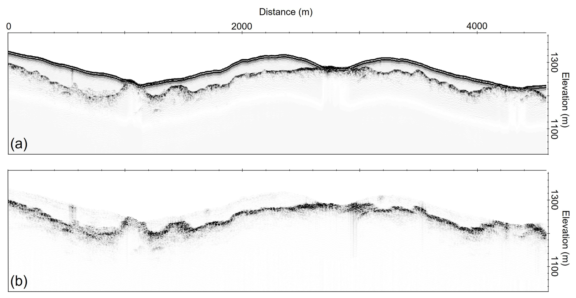
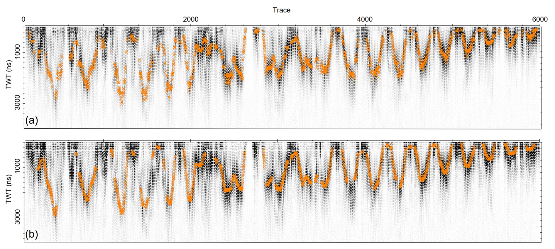
Table D1 Measured dGNSS point elevations for MG, RG, and RIV. Point elevations for SG are not included due to the lack of dGNSS measurements there in 2024. The coordinates were recorded in the SWEREF 99 TM system.

Appendix E

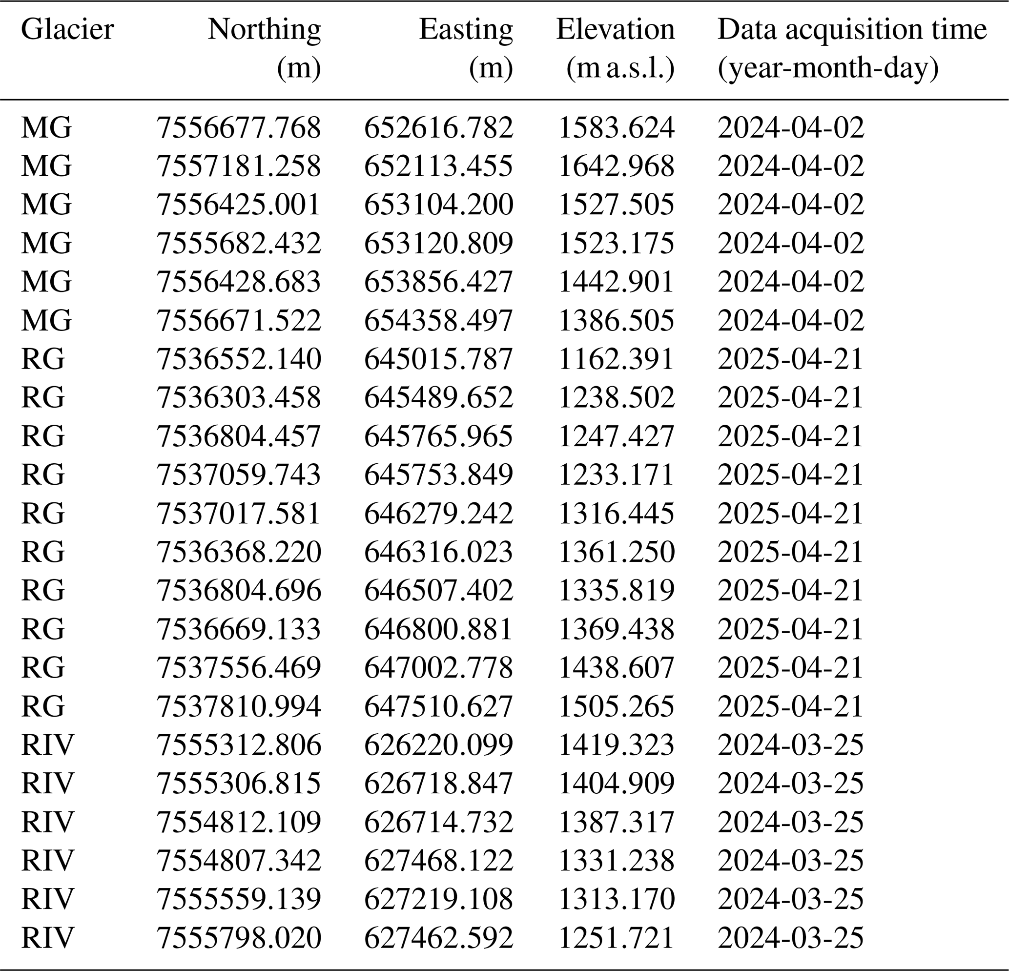
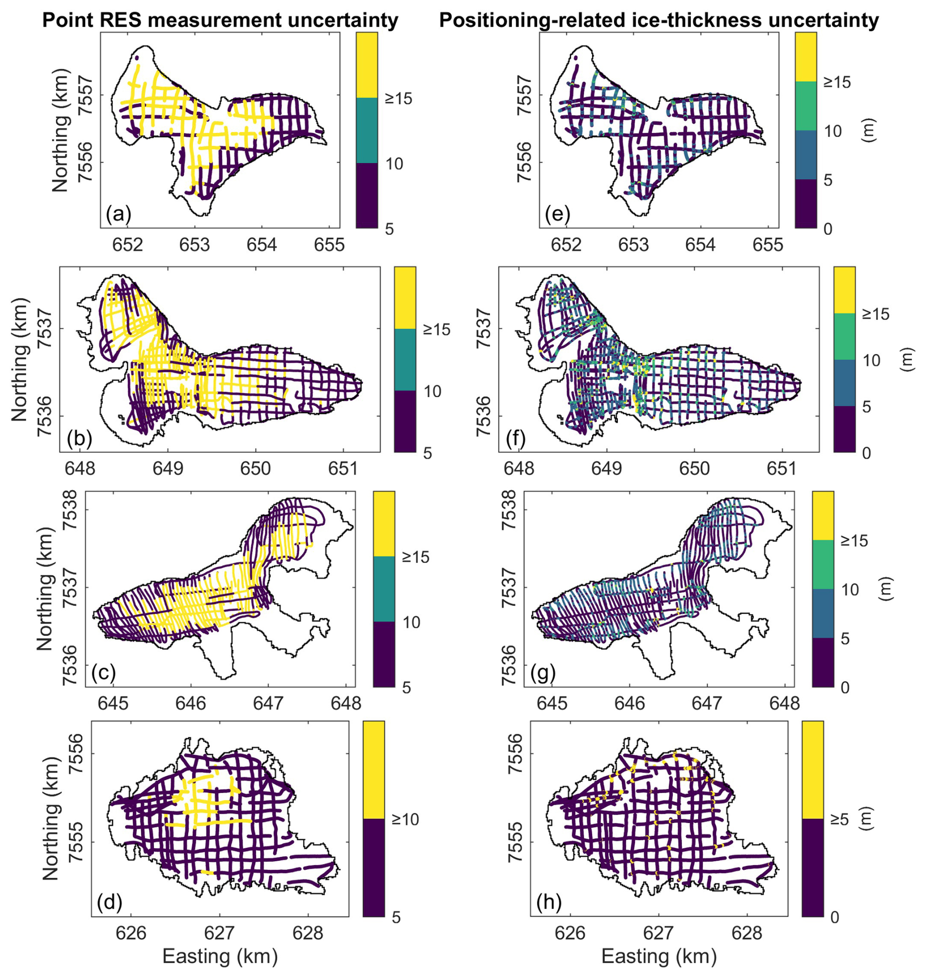
Figure E1 Point RES measurement uncertainty (a–d) and positioning-related ice-thickness uncertainty (e–h) for MG, RG, SG, and RIV, respectively.

Appendix F

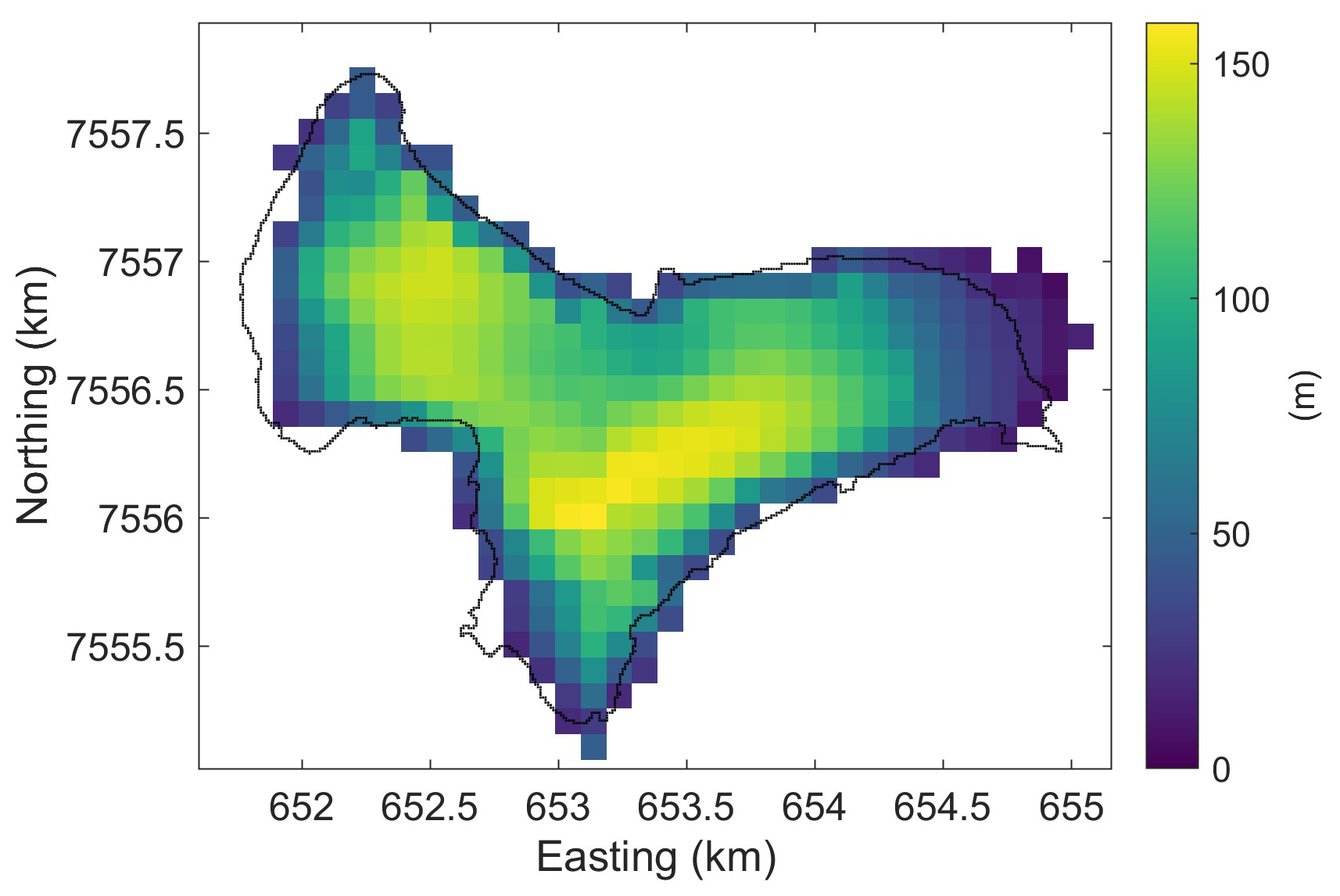
Figure F1 Updated modelled ice thickness for MG. The experiment follows that of Frank and van Pelt (2024), except that RES-measured ice thicknesses were introduced as constraints for global modelling parameters.