Field measurements of hydrodynamics and sediment transport at intertidal areas in the Dutch Wadden Sea

Two field measurement campaigns were carried out in the Dutch Wadden Sea in winter 2023–2024 and in early spring 2025. The campaigns were designed to understand and quantify sediment transport and exchange at two different spatial scales: on larger scale between two adjacent tidal basins and on smaller scale between individual channels and shoals.

The presented dataset contains point measurements at five locations in the first campaign and eight locations in the second campaign, including (1) near-bed flow velocities and velocity profiles, (2) wave characteristics, (3) suspended sediment concentrations and transport rates, and (4) local bed level dynamics, as well as data on the sediment composition of (intertidal) seabed samples. Measurements were collected simultaneously for a period of six to eight weeks in both campaigns, although some instruments collected data for only four weeks in the Winter 2023–2024 campaign.

This article documents the field observations and data processing, and highlights potential applications. The dataset is collected for a better understanding of sediment dynamics in the Dutch Wadden Sea, but also to advance our understanding of channel-shoal sediment exchange mechanisms in general. The field data enables the investigation of fundamental processes controlling sediment dynamics in tidal systems, such as tide- and wind-driven flows and transport, shallow water wave dynamics, wave and current-induced resuspension, and sediment bed stability.

The data are publicly available in three versions (raw, filtered and tailored datasets) at 4TU Centre for Research Data at https://doi.org/10.4121/bbb85feb-15f9-476f-9598-b6509392117d (van Weerdenburg et al., 2026).

1 Introduction

The morphology of coastal and estuarine systems evolves through the continuous supply, transport, and redistribution of sediment from both marine and fluvial sources (Syvitski et al., 2022). These dynamics are shaped by natural forcing as well as human interventions (e.g., Wang et al., 2015; Blum and Roberts, 2009; Eslami et al., 2019; Nienhuis et al., 2020). Both sediment surpluses and deficits pose challenges to coastal functions, including flood protection, ecological value, and the accessibility of ports and waterways, highlighting the need for efficient sediment management. Sustainable sediment management strategies, such as nourishment schemes and dredging practices, rely on a thorough understanding of the fundamental processes governing sediment dynamics. This knowledge must be translated to the spatial and temporal scales relevant for coastal (sediment) management (Wang et al., 2012), as coastal and estuarine morphology evolves through processes operating across multiple, interdependent spatiotemporal scales (De Vriend, 1991a, b; Cowell et al., 2003a, b). Morphological features such as channels and shoals may represent individual units at one scale but are components of larger systems, including estuaries or tidal basins, at another. While the monitoring of some activities can be effectively addressed at a single scale, many are influenced by cross-scale interactions. For example, maintenance dredging of a tidal channel is typically monitored using its dredging volume, but understanding processes controlling siltation (and thus dredging volumes) requires understanding of sediment supply (i.e., at larger spatiotemporal scales), sediment transport mechanisms (i.e., at local or larger scales), and sediment properties (i.e., at smaller scales).

In the Dutch Wadden Sea, evolution on large spatiotemporal scales is addressed using extensive long-term monitoring networks maintained by the Dutch Ministry of Infrastructure and Water Management. However, analyses of processes at smaller spatial and temporal scales – such as sediment transport between channels and shoals requires more frequent and detailed observations of hydrodynamics, sediment transport and morphodynamic development. Existing datasets insufficiently cover sediment exchange mechanisms within and between channel-shoal systems, which motivated the initiation of two extensive field campaigns that are presented in this article. These field campaigns build on regular monitoring programs and several earlier field campaigns in the Dutch Wadden Sea. Sediment transport measurements over fringing muddy tidal flats are presented by Colosimo et al. (2020, 2023), following three field campaigns in 2016–2018. Observations reveal an important role for wind-driven flows in addition to wave-induced resuspension, and suggest the temporal storage of (fine) sediment on mudflats during calm weather conditions. Van Prooijen et al. (2020) present a dataset obtained by an extensive field campaign focused on one of the ebb-tidal deltas in the Dutch Wadden Sea, accompanied by measurements of water levels and flow velocities at two tidal divides (van Weerdenburg et al., 2021). The dataset provides evidence for the significant wind-driven exchange flows between basins found in process-based numerical model results by Duran-Matute et al. (2016), but does not contain sediment transport measurements inside the tidal basins. Van Maren et al. (2023) present a field dataset on sediment dynamics and exchange mechanisms between the tidal river and the outer estuary in one of the estuarine channels in the Wadden Sea (the Ems estuary), thereby focusing on the sediment dynamics in a relatively deep part of the coastal system that is more strongly influenced by baroclinic processes.

Despite the regular monitoring and earlier campaigns, integrated observations of sediment transport across the larger channel-shoal system remain lacking. We therefore designed two complementary field campaigns with the following two objectives. The first objective is to collect detailed measurements of sediment transport across tidal divides, providing quantitative insight into sediment exchange between basins. The second objective is to obtain combined measurements of flow, waves, sediment transport, and bed-level dynamics in a channel–shoal system, enabling a better understanding of the mechanisms that govern channel–shoal sediment exchange. Given the large amount of measurement locations and instruments, we believe the obtained dataset not only advances our understanding of sediment dynamics in the Dutch Wadden Sea, but potentially also improves generic process understanding relevant for channel-shoal systems worldwide (e.g., in the Yangtze Estuary and along the Jiangsu Coast (China), in San Francisco Bay (USA), and the Venice Lagoon (Italy)). This article describes the design of the data collection campaigns, the processing of the data, and an overview of the available dataset. The dataset is published as the WadSED dataset, as the field campaigns were initiated within the WadSED (https://wadsed.nl, last access: 17 June 2026) project.

2 The Dutch Wadden Sea

The Wadden Sea is an interconnected system of 39 tidal basins and estuaries that stretches roughly 500 km along the coast of the Netherlands, Germany, and Denmark. Its Dutch and German parts were appointed as UNESCO World Heritage Site in 2009, followed by the Danish part in 2014 (UNESCO World Heritage Committee, 2014). In the Dutch Wadden Sea (Fig. 1), the tidal range increases from about 1.4 m near the westernmost inlet (the Marsdiep Inlet) to 2.6 m at the mouth of the Ems estuary in the east. The tidal inlets are classified as mixed-energy tide-dominated systems (Davis and Hayes, 1984; Wang et al., 2012), reflecting their large tidal prisms and relatively low wave energy (Elias et al., 2012). Wave conditions within the basins are dominated by locally generated short-period (≤ 4–5 s) wind waves, constrained by the fetch or the local water depth. Offshore waves (mean significant wave height of 1.3 m, typically from the west-southwest, and mean wave period of 5–6 s; Elias et al., 2012; Ridderinkhof et al., 2016) hardly propagate through the tidal inlets. Wind conditions are predominantly from the southwest to west (Fig. 3). There is a pronounced seasonal variability in wind and storm activity, with most storm events occurring between late autumn and early spring. The interannual variability in wind conditions is primarily associated with changes in wind direction rather than in total wind energy (Gerkema and Duran-Matute, 2017).

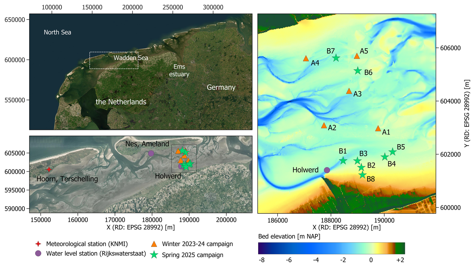
Figure 1 Maps showing the measurement locations in the two field campaigns in the Dutch Wadden Sea, south of the Ameland barrier island, and nearby permanent meteorological and water level stations. Basemap sources: Esri World Imagery | Powered by Esri (top left panel), PDOK (bottom left panel), and bed elevation data relative to NAP (Netherlands Ordnance Datum; right panel; Rijkswaterstaat, 2026).

The morphology of the Dutch Wadden Sea is highly dynamic and characterized by bifurcating channel networks separated by shallow, often intertidal, flats (Wang et al., 2012; Cleveringa and Oost, 1999). Channel depth generally decreases in landward direction, from several tens of meters in tidal inlets to a few meters in the back-barrier basins. The channel networks of adjacent tidal inlets are interconnected in the western part of the Dutch Wadden Sea, whereas they end in shallow areas known as tidal divides in the eastern part (Fig. 1). The bed is generally sandy close to the tidal inlets, becoming more muddy towards the tidal divides and mainland coast in the back of the basins (e.g., Folmer et al., 2023; Colina Alonso et al., 2024). Following large-scale human interventions in the 20th century, most notably the closure of the Zuiderzee in 1932 and the Lauwerszee in 1969, the Dutch Wadden Sea has imported large amounts of sediment, leading to the infilling of channels and accretion of intertidal areas (Wang et al., 2018; Elias et al., 2012; Colina Alonso et al., 2021). At present, extensive dredging is carried out to maintain the fairways to the barrier islands and the North Sea (2×10⁶–3×10⁶ m³ yr⁻¹ in the Dutch Wadden Sea excluding the Ems estuary and port maintenance dredging), reflecting the generally high sediment availability in the system.

3 Field observations

3.1 Overall design

The two field campaigns were designed to understand and quantify sediment exchange at two different spatial scales: (1) between different basins, and (2) between channels and shoals within a basin. These objectives steer (i) the spatial design, (ii) measurement period, (iii) measurement duration, and (iv) instrumentation. These design aspects and the installation of the measurement frames are explained in greater detail below, followed by more detailed descriptions of the content of the resulting Winter 2023–2024 and Spring 2025 campaigns in the next sections.

All measurements were carried out south of a barrier island (Ameland) centrally located in the Dutch Wadden Sea (Fig. 1). The scientific motivations to select this part of the Wadden Sea were (1) the presence of channel-shoal transitions in close proximity to a tidal divide; (2) the large spatial variation of sandy and muddy sediment beds, with the northern part of the basin being generally sandier and the southern part muddier (Bijleveld et al., 2025); and (3) the influence of anthropogenic activities, including frequent dredging of the navigation channel and associated sediment disposal in the basin, such that sediment dynamics are controlled by both natural and anthropogenic processes. Practical considerations include the accessibility of the site via the Holwerd ferry pier and the Ameland marina, and the availability of complementary data from other monitoring campaigns and programs (discussed in Sect. 5). The Winter 2023–2024 campaign (A stations in Fig. 1) was primarily done to better understand the spatial variability in flow and sediment transport between two basins, hence we selected the measurement locations around the tidal divide and located in both the west- and eastward basin. The Spring 2025 campaign (B stations in Fig. 1) was done to further improve our understanding of the exchange between basins, but also to better understand the (fine-)sediment exchange processes between channel and shoals in the south of the tidal basin. All measurement locations were focused on the back of the basin near the tidal divide, thereby prioritizing a detailed investigation of this area at the expense of capturing the full spatial variability of intertidal areas across the basin.

The key factor controlling the selection of the measurement period was the seasonal variability in wind climate. Wind induces (residual) flow across tidal divides (Duran-Matute et al., 2016; van Weerdenburg et al., 2021), and wave stirring mobilizes sediment on tidal flats (Green and Coco, 2014; Colosimo et al., 2020). To sample both storm-driven dynamics (when transport over the tidal divides and erosion of the tidal flats are expected) and calm-weather conditions (typically characterized by accreting tidal flats), both measurement campaigns were scheduled at transitional periods: at the beginning of winter (the Winter 2023–2024 campaign; Sect. 3.2) and spring (the Spring 2025 campaign; Sect. 3.3). The summer season is not captured in the two measurement campaigns, such that effects of biota on sediment dynamics that peak in summer (e.g., Van Der Wal et al., 2010) are not included in the data.

The duration of measurement campaigns reflect a trade-off between deployment duration and sampling frequency, constrained by instrument battery capacity. Extending deployments through servicing was not feasible for practical and financial reasons. Deployment and retrieval were further limited to periods with sufficient emergence of the intertidal measurement locations during daylight hours. For both campaigns, the duration of measurements amounted to approximately 8 weeks.

Measurement locations were equipped with a selection of instruments to measure flow velocities, waves, suspended sediment concentrations, and the local bed level, although not all parameters could be measured at every location due to the limited availability of instruments. Flow velocity profiles were measured with Acoustic Doppler Current Profilers (ADCPs). Acoustic Doppler Velocimeters (ADVs) were deployed for high-frequent measurements of flow velocities (capturing the oscillatory near-bed flows generated by waves) and water level variations. The ADVs were mounted vertically, such that they also measure the distance to the bed, hence the variation in bed elevation, at the start and end of each burst. The acoustic backscatter of the ADVs may be used as a measure for the suspended sediment concentration (SSC) (Pearson et al., 2021), but all measurement locations were also equipped with at least one optical backscatter sensor (OBS) to determine the turbidity, used to estimate the SSC (see Sect. 3.5). Local water levels are derived from the pressure measurements of ADCP and ADV instruments. Some of the measurement stations in the second (Spring 2025) campaign were equipped with an A-SED (Willemsen et al., 2022; Xu et al., 2023) for acoustic measurements of the distance to the bed, similar to the ADV bed level measurements but carried out at an acoustic frequency of 400 kHz instead of 6 MHz. Hourly atmospheric pressure measurements at the permanent meteorological measurement station at Hoorn, Terschelling (Fig. 1) are available to correct pressure recordings for variations in atmospheric pressure. During the Spring 2025 campaign, however, we installed a pressure sensor in Holwerd (i.e., closer to the measurement site).

Most measurements stations were installed on intertidal areas, where frames and instruments were mounted in situ during low tide, when the seabed was exposed. Locations on a fringing mudflat were accessed on foot from the Holwerd ferry pier. The other intertidal locations (Fig. 1) were reached by grounding a ship (prior to low tide) followed by transport on foot, with materials transported on (floating) sledges. All frames were marked with surface buoys. The single subtidal station (Spring 2025 campaign) was installed by lowering an instrumented lander from a vessel during high tide. The lander was secured in position using a weighted anchor and marked with multiple surface buoys. A series of photographs in Fig. 2 illustrates the installation of the measurement stations.

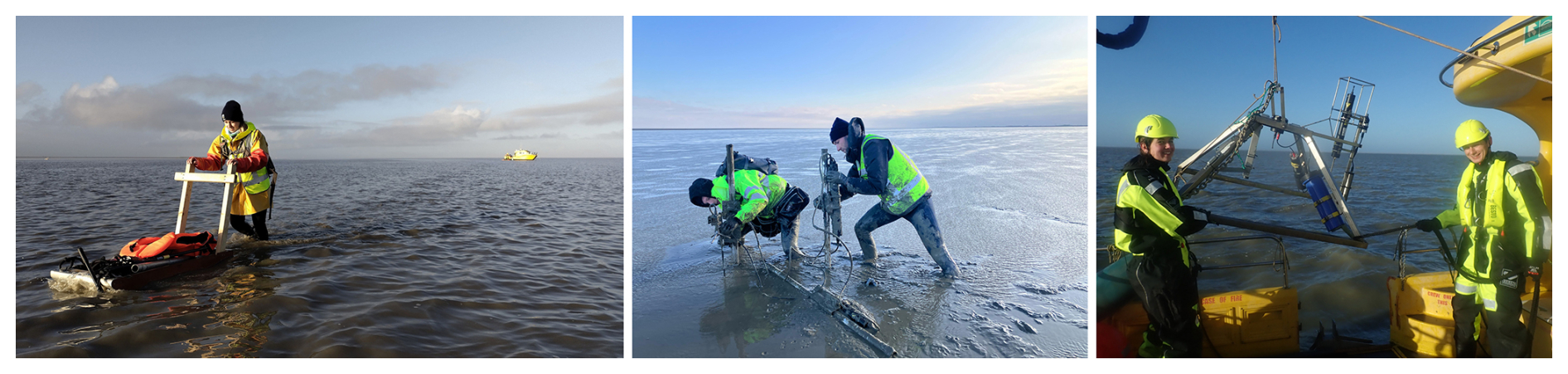
Figure 2 Photographs illustrating the installation of the measurement stations. Left: transport of instruments and equipment to intertidal measurement locations, after vessel grounding. Middle: in situ assembly of a scaffold frame equipped with instruments on a fringing mudflat. Right: deployment of an instrumented lander from a vessel.

3.2 The Winter 2023–2024 campaign

The measurement stations in the Winter 2023–2024 campaign were installed on 21 November 2023, and retrieved on 16 January 2024. The observed wind conditions over this period are illustrated in Figs. 3 and 4a and the water level variation at a nearby (permanent) measurement station (Nes) is illustrated in Fig. 4b. Winds were relatively strong during the measurement period (mean wind speed 7.7 m s⁻¹ compared to an average wind speed of 6.2 m s⁻¹) and frequently directed from the west (Fig. 3). Winds from the northern and southern quadrants were hardly observed. The passing of four storms (Elin on 9 December, Pia on 21 December, Gerrit on 27 December, and Henk on 2–3 January) caused multiple periods with strong winds during the observation period (with the maximum observed hourly mean wind speed exceeding 20 m s⁻¹ on 3 January) and elevated water levels. Storm Pia on 21 December induced an exceptionally high water level set-up along the Dutch coast, such that all storm surge barriers in the Netherlands were closed for the first time ever. The resulting water levels in the Dutch Wadden Sea (3.19 m NAP at Nes; Fig. 4) were the highest since 2006.

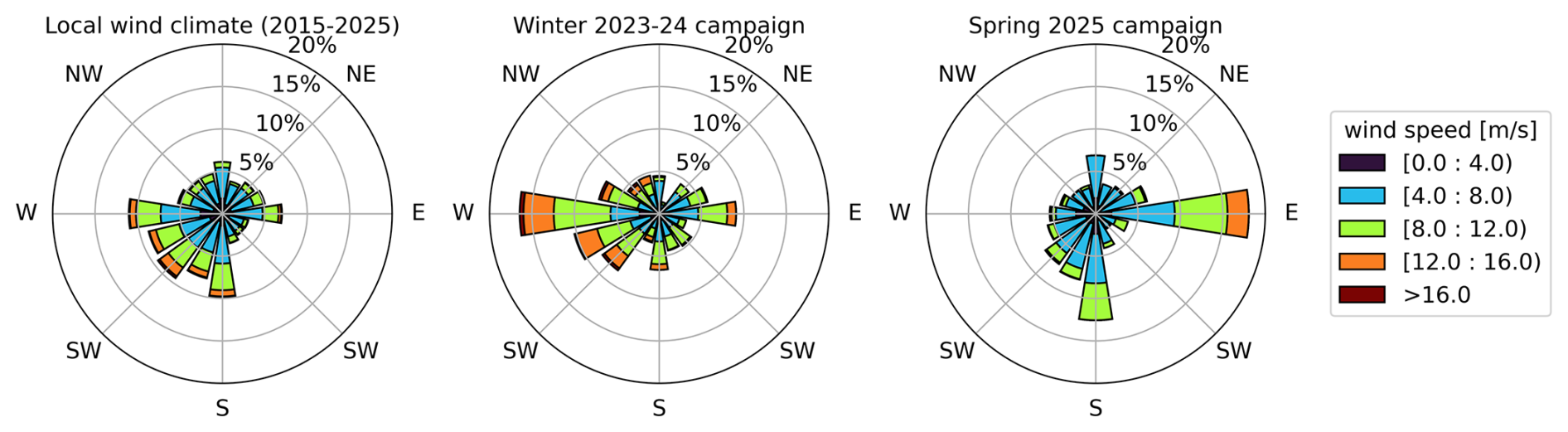
Figure 3 Wind roses showing the observed wind conditions at Hoorn, Terschelling for the past 10 years (left), the Winter 2023–2024 campaign (middle), and the Spring 2025 campaign (right).

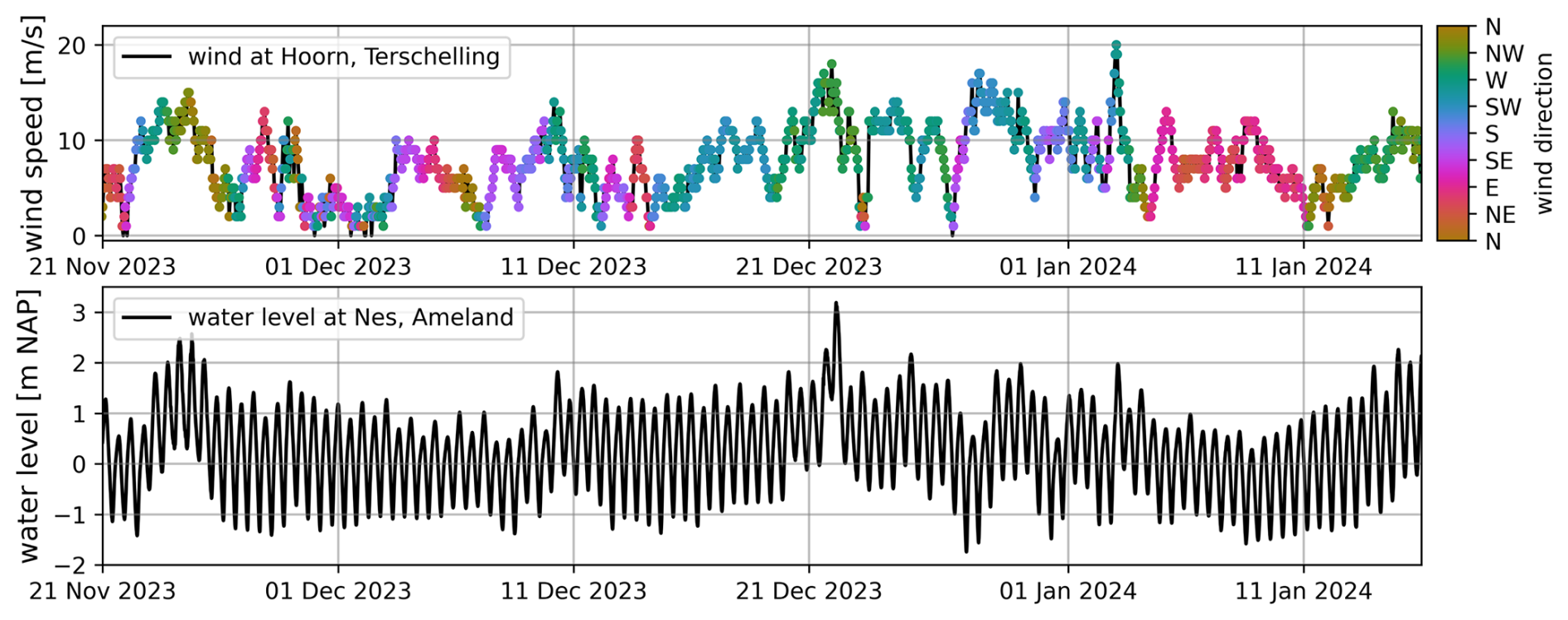
Figure 4 Observed wind conditions (at Hoorn, Terschelling; top panel) and water levels (at Nes, Ameland; bottom panel) during the Winter 2023–2024 campaign.

Measurement stations A2 and A4 were located on the shoals along two different channel distributaries in the basin west of the tidal divide of Ameland (Fig. 1). Stations A1 and A3 were located on the tidal divide, in between the channel ends of both tidal basins. Station A5 was located just east of the tidal divide. Each measurement station was equipped with an upward looking ADCP (Nortek Aquadopp Profiler) and a sideward looking OBS (Campbell OBS-3+ Turbidity Sensor). The ADCPs were placed within the seabed, with only the head of the instrument emerging above the bed (Fig. 5), allowing flow velocity measurements in relatively shallow water. The OBSs were mounted such that their measurement height corresponds to the lowest bin of the ADCPs. In addition, stations A2, A3 and A4 were equipped with a downward looking ADV (Nortek Vector). Unfortunately, the five ADCP + OBS sets stopped measuring after approximately one month because of power failures. Further details of the deployment and the configuration of the different instruments are listed in Table 1.

Table 1 Instruments and their configuration at the measurement stations in the Winter 2023–2024 campaign. Multiple elevations indicate the elevation of the various connected instruments (e.g., first value for the AQD, second for the OBS). The number in brackets denotes the elevation of the ADV pressure sensor; note that the ADV measurement volume is located 15 cm below the instrument.

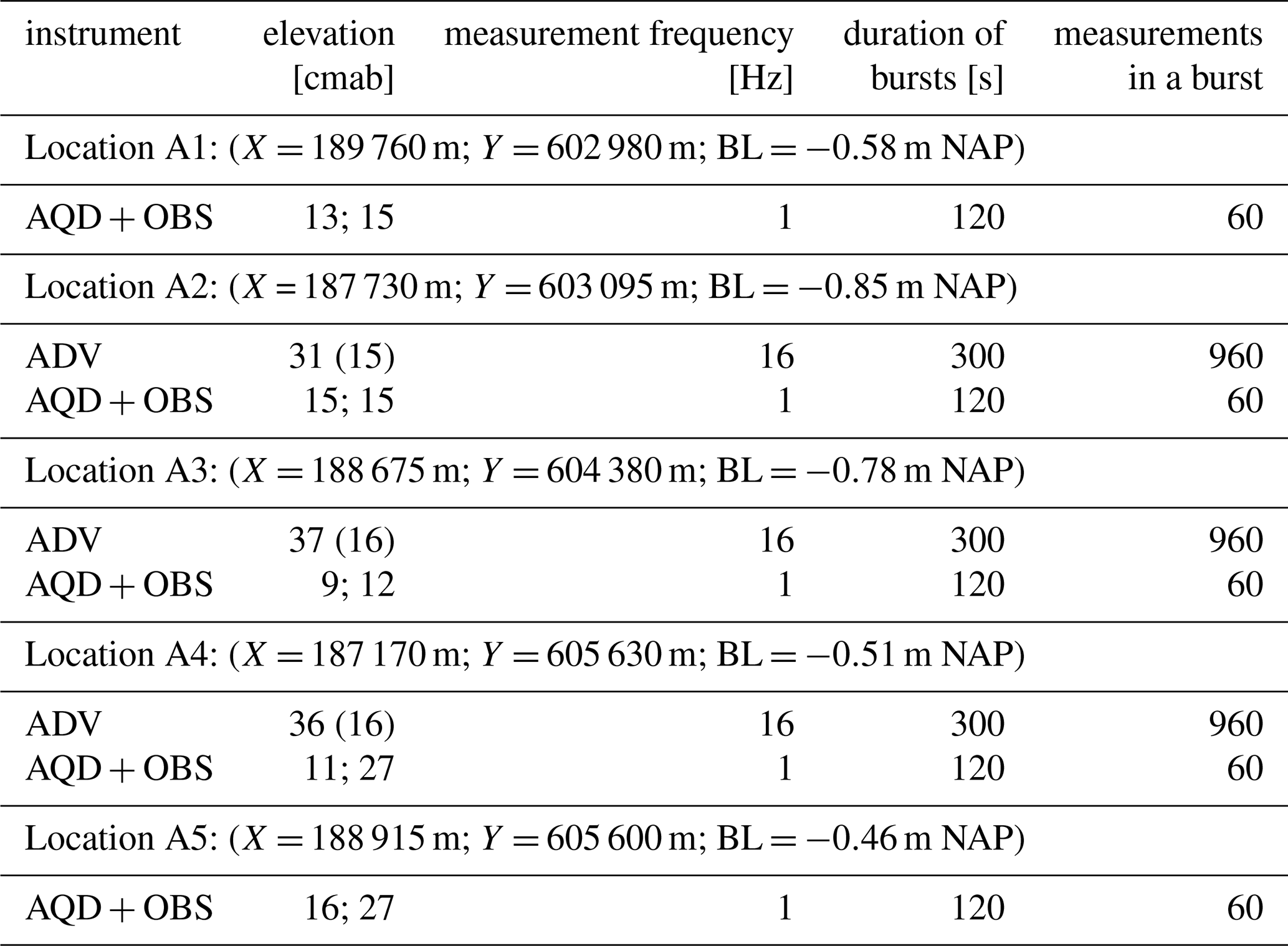
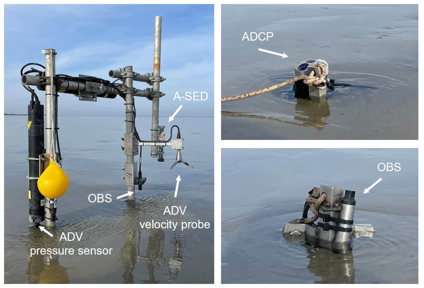
Figure 5 Photographs illustrating the instrumentation of intertidal measurement stations. Left: one of the scaffold frames, equipped with an ADV, OBS, and A-SED. Right: ADCP (Aquadopp Profiler) and OBS, mounted within the seabed.

3.3 The Spring 2025 campaign

The measurement stations in the Spring 2025 campaign were installed on 27 and 28 January (locations B6 & B7), on 6 and 7 February (B1–B5), and on 13 February (B8), 2025, and retrieved on 26–31 March 2025. The observed wind conditions over this period are illustrated in Figs. 3 and 6a and the water level variation at a nearby (permanent) measurement station (Nes) is illustrated in Fig. 6b. During most of the measurement period, winds were relatively weak (<10 m s⁻¹) and from varying directions. The strongest winds of approximately 14 m s⁻¹ were from the east, which is exceptional when comparing to the average wind climate (i.e., strong winds from the east are uncommon), causing a water level set-down exceeding 1 m at the measurement site.

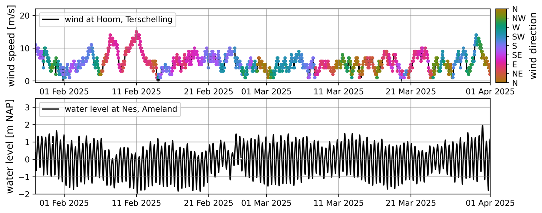
Figure 6 Observed wind conditions (at Hoorn, Terschelling; top panel) and water levels (at Nes, Ameland; bottom panel) during the Spring 2025 campaign.

Measurement stations B5, B6 and B7 were located at the tidal-divide (Fig. 1), with the bed elevation (at deployment) ranging from −0.77 m NAP to −0.56 m NAP (Table 2). Station B1 was located at the end of a tidal channel. Stations B2–B4 and B8 were located on the fringing mudflat adjacent to this channel, with stations B3, B2, and B8 in a transect from the channel edge towards the salt marsh. Each station was equipped with an upward-looking ADCP (Nortek Signature, Aquadopp Profiler, or HR Profiler), either mounted on a frame or placed within the seabed, and one (B7), two (B1, B3–B6 and B8) or three (B2) turbidity sensors (Campbell OBS-3+, Seapoint STM, or WiMo turbidimeter). Frame-mounted ADVs (Nortek Vector) were installed at all stations except B7 (Fig. 5), with A-SEDs (Willemsen et al., 2022; Xu et al., 2023) at stations B1, B2, B5, B6 and B8. The two WiMo Multiparameter Sondes (MPP) at B1 were not only logging turbidity, but also conductivity and water temperature. Configurations of frames and instruments varied slightly among the stations due to equipment availability. Full details are provided in Table 2.

Table 2 Instruments and their configuration at the measurement stations in the Spring 2025 campaign. The number in brackets denotes the elevation of the ADV pressure sensor; note that the ADV measurement volume is located 15 cm below the instrument.

^* Location B6 was equipped with an Aquadopp HR Profiler instead of an Aquadopp Profiler.

3.4 Sediment bed composition

Bed sediment samples were collected during both campaigns at all measurement locations except from A1, A5, and B1, to determine the (dry) sediment density and grain size distribution (GSD), and for the Spring 2025 campaign also the organic content and shell material fraction. The samples were taken by filling 50 mL jars with sediment from the top ± 2 cm of the seabed. Wet and dry densities (Table 3) are determined based on the loss of mass after (overnight) drying in the oven at a temperature of 105 °C, assuming a water density of ρ_w=1025 kg m⁻³ and a density of solids of ρ_sol=2600 kg m⁻³.

Table 3 Sediment bed density and composition at the measurement locations; no sediment samples were collected at locations A1, A5, and B1. The fractions p_silt and p_clay correspond to sizes <4 and 4–63 µm, respectively, and $p_{\mathrm{sand}}=\mathrm{100}\mathit{\%}-p_{\mathrm{silt}}-p_{\mathrm{clay}}$. The numbers in brackets represent the results of grain size analysis of Spring 2025 samples after removal of shell fragments with HCl. %OM and %CaCO₃ were not determined for the Winter 2023–2024 campaign's samples.

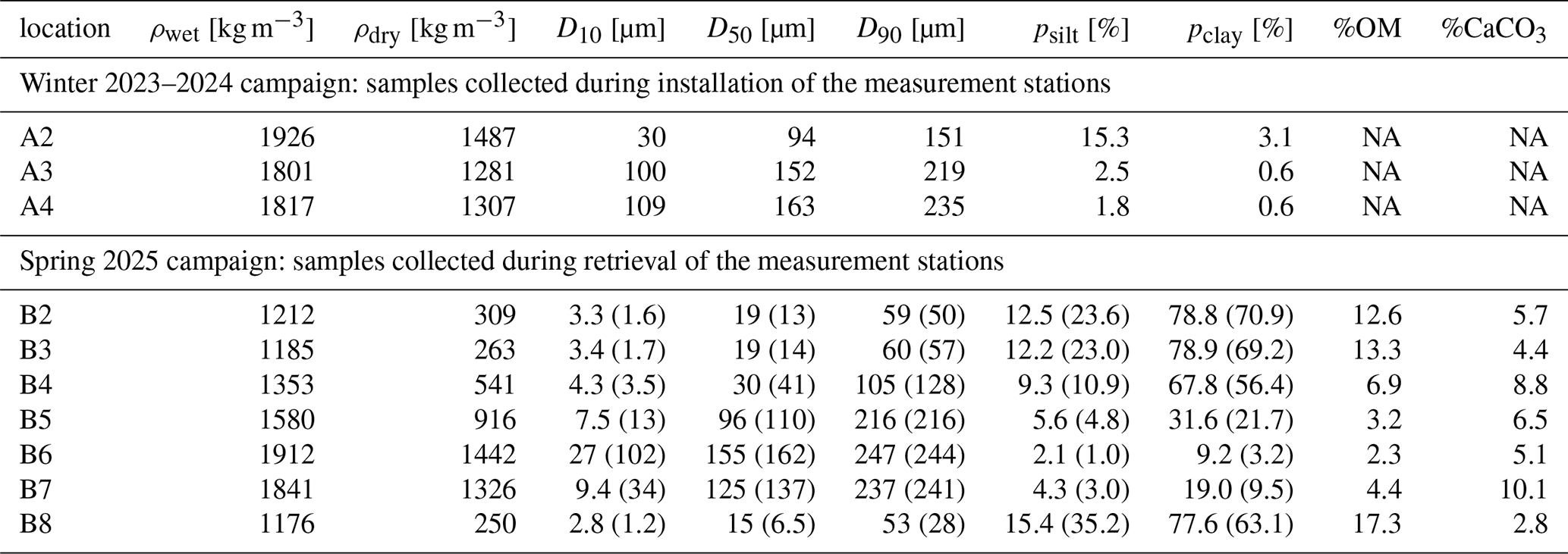
NA – not available.

The grain size distribution (GSD) of the dried samples of the Winter 2023–2024 campaign was determined using a Malvern Mastersizer 3000 after pre-treating the samples using a combination of deflocculant (Na₄O₇P₂⋅10H₂O) and ultrasone. Two subsamples of the Spring 2025 samples were analysed for GSD using a Malvern Mastersizer 2000, one without and one with treatment with HCl (1 mol L⁻¹) to remove shell fragments. A third subsample was analysed with a TGA701 Thermogravimetric Analyzer for the organic content and the (mass) fraction of carbonate minerals. The fraction organic matter (%OM) and carbonate minerals (%CaCO₃) are computed from the loss of sample mass during heating as follows:

$$\begin{array}{}\text{(1)}& {\displaystyle }\text{\%OM}={\displaystyle \frac{m_{\text{dry}}-m_{\mathrm{550}\mathrm{°}\mathrm{C}}}{m_{\text{dry}}}}\cdot \mathrm{100}\text{(2)}& {\displaystyle }\begin{array}{rl}& {\text{\%CaCO}}_{\mathrm{3}}={\displaystyle \frac{m_{\mathrm{550}\mathrm{°}\mathrm{C}}-m_{\mathrm{800}\mathrm{°}\mathrm{C}}}{m_{\text{dry}}}}\cdot {\displaystyle \frac{M_{{\text{CaCO}}_{\mathrm{3}}}}{M_{{\text{CO}}_{\mathrm{2}}}}}\cdot \mathrm{100},\\ & {\displaystyle \frac{M_{{\text{CaCO}}_{\mathrm{3}}}}{M_{{\text{CO}}_{\mathrm{2}}}}}={\displaystyle \frac{\mathrm{100.09}}{\mathrm{44.01}}}\approx \mathrm{2.273}\end{array}\end{array}$$

with m_dry the mass of the sampling after drying at 105 °C, m_550 °C and m_800 °C the mass of the sample after heating the sample until 550 and 800 °C, respectively, and $M_{{\text{CaCO}}_{\mathrm{3}}}$ and $M_{{\text{CO}}_{\mathrm{2}}}$ the molar mass of CaCO₃ and CO₂ in [g mol⁻¹]. Several characteristics of the sediment samples are listed in Table 3, indicating the muddy (clayey) measurement locations in the south and sandy measurement locations towards the north of the tidal basin.

3.5 Calibration of turbidity sensors

The OBS turbidity sensors were calibrated in a tank using suspensions with known sediment concentrations to convert the analogue sensor output to suspended sediment concentration (SSC). Calibration suspensions, ranging from clear water to 8000 mg L⁻¹, were prepared from local bed samples from locations B3 and B4 (with p_sand = 9 %–23 % and p_mud = 91 %–77 %; Table 3), because collecting water samples during deployment and retrieval was not feasible at intertidal measurement locations. Instrument-specific calibration curves are derived by fitting a linear relationship between the OBS signal (in counts or mV) and SSC (in mg L⁻¹) at low SSC, and a quadratic relationship at higher SSC. Figure 7 illustrates the calibration curves for the Seapoint STM and Campbell OBS-3+ deployed at location B3. The OBS-3+ has a linear response up to approximately 1000 mg L⁻¹, whereas the STM remains linear up to about 1500 mg L⁻¹. At SSC > 4000 mg L⁻¹, the STM backscatter intensity decreases for increasing SSC, indicating that concentrations exceed the instrument's reliable operating limit.

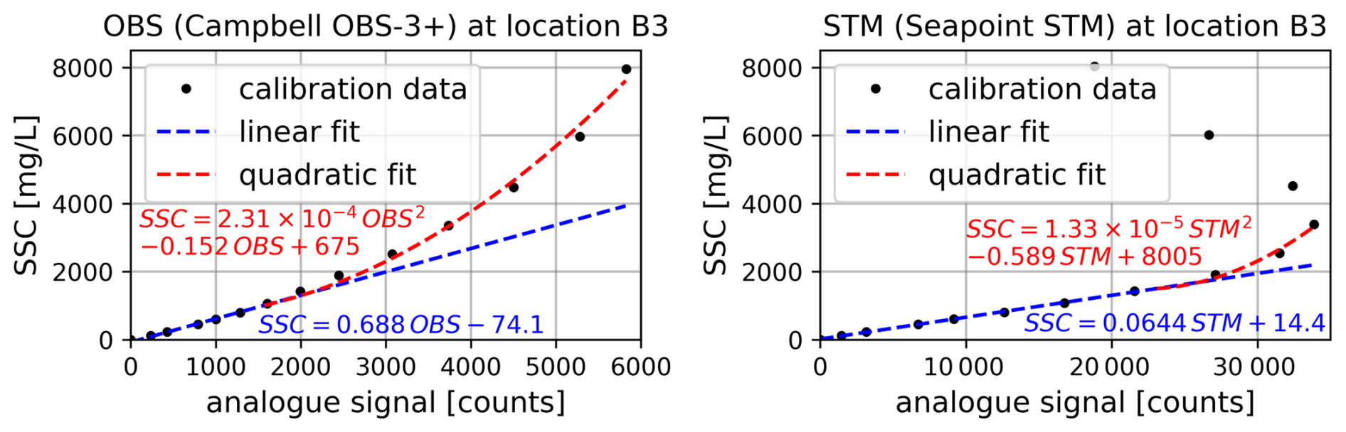
Figure 7 Examples of calibration curves of OBS (left) and STM (right) turbidity instruments deployed at location B3. The transition between the linear and quadratic calibration curves is at 1000 mg L⁻¹ for the OBS and at 1500 mg L⁻¹ for the STM.

4 Data processing

The in situ measurement data is made available in three versions, reflecting different processing stages: (1) raw data from the different instruments, converted into standardized NetCDF format; (2) filtered data, in which measurements that do not satisfy quality requirements are removed; and (3) tailored data, with (burst-averaged) characteristic quantities. Processing of the raw data into the filtered and tailored dataset is carried out with a collection of Python scripts that largely builds upon the processing of field measurements with a similar set of instruments by Van Der Lugt et al. (2024), as is discussed in the next sections. Figure 8 summarizes the data availability after quality assurance, as included in the filtered and tailored datasets.

Figure 8 Overview of the data availability after quality assurance, for the Winter 2023–2024 campaign (top panel) and the Spring 2025 campaign (bottom panel). ¹ High-frequent (wave-induced) pressure fluctuations were not captured at station A4 due to a malfunctioning ADV pressure sensor. ² Aquadopp Profiler velocity measurements at station A4 are unreliable due to one malfunctioning acoustic beam. ³ Water levels at B6 are derived from HR Profiler pressure measurements rather than the ADV, due to drift in the ADV pressure signal during the final three weeks of the campaign.

4.1 Pressure measurements

Burst-averaged pressure measurements from ADVs and ADCPs are used to determine the local water level, and the high frequent (16 Hz) ADV pressure measurements are used to determine wave spectral statistics (as discussed in Sect. 4.3). The pressure is converted into a water level in two steps. First, the offset of the different pressure sensors follows from the difference between the recorded pressure and the atmospheric pressure at a moment at which the instruments are not immersed (t_ref, typically the first low-water period after deployment), and is subtracted from the data. Next, the pressure recordings are corrected for atmospheric pressure variations, by subtracting the recorded atmospheric pressure relative to t_ref. The water depth above the pressure sensors is determined by dividing the air-pressure corrected recordings with the mean water density (ρ=1025 kg m⁻³) and the gravitational acceleration (g=9.81 m s⁻²), and yields the local water level after adding the measured elevation of the pressure sensors in the field.

During emerged conditions, some of the pressure recordings from our ADVs and ADCPs were obviously erroneous (> several kPa). The pressure sensors in these instruments are temperature-compensated, and we expect the errors were caused by rapid, uneven heating of the instruments during sunny days, or cooling during cold nights (i.e., when the air temperature is significantly different from the water temperature; Fig. 9). Hence, the pressure data could not reliably indicate the periods of inundation of the instruments. Low-water periods are therefore removed from the data based on the amplitude of the acoustic signal of the velocity measurements, which is (too) low when the instruments were not immersed. Low-water periods are removed from the ADCP data by applying a minimum amplitude threshold in the lowest velocity bin (see Sect. 4.2).

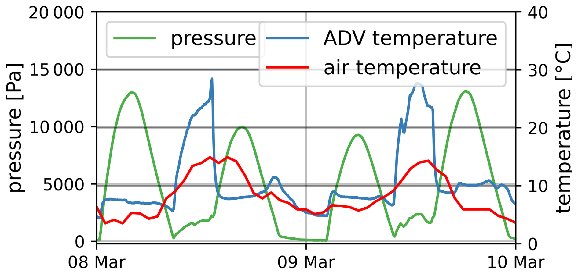
Figure 9 Example of erroneous ADV pressure recordings during emerged conditions (the air-pressure-corrected pressure signal deviates from zero), when the internal temperature of the instrument deviates from the air temperature.

4.2 Flow velocity measurements

Processing of the ADV and ADCP velocity measurements consists of three steps: (1) filtering outliers; (2) excluding data from periods when the instruments, or, for ADCPs, individual velocity bins, were not immersed; and (3) converting velocities from probe coordinates (XYZ) to field coordinates (ENU).

ADV recordings are flagged as outliers if the instantaneous inter-beam correlation does not exceed 62 %, if the instantaneous velocity exceeds the instrument's velocity range, or if the instantaneous measurements are more than 3 standard deviations from the mean over a burst. The correlation threshold of 62 % follows from the criterion proposed by Elgar et al. (2001):

$$\begin{array}{}\text{(3)}& c_{min}=\left(\mathrm{0.3}+\mathrm{0.4}\cdot \sqrt{{\displaystyle \frac{s_{\mathrm{f}}}{s_{\mathrm{f}\mathrm{0}}}}}\right)\cdot \mathrm{100}\mathit{\%}\end{array}$$

with s_f the sampling frequency of ADV measurements of 16 Hz and s_f0 the reference frequency of this criterion of 25 Hz. The horizontal and vertical velocity range of 3.5 and 1 m s⁻¹, respectively, follow from the nominal velocity range of ±2.0 m s⁻¹ that is set while programming the ADVs. The ADCP measurements are processed with a minimum inter-beam correlation threshold of 50 %, which satisfies the criterion for acceptable measurement accuracy by Elgar et al. (2005) for the sampling frequency of 1 Hz. Only the burst-averaged ADCP measurements are included in the filtered and tailored datasets. The almost continuous Aquadopp HR Profiler measurements at location B6 are averaged over 10 min intervals.

Low-water periods, during which instruments were not submerged, are excluded from the dataset based on the acoustic signal amplitude rather than the local water level, as pressure recordings during emerged conditions proved to be unreliable (see Sect. 4.1). For the ADVs, low-water periods were defined as intervals where the burst-averaged signal-to-noise ratio (SNR) did not exceed 10 dB (Fig. 10). For the Aquadopp (HR) Profiler ADCPs, a beam amplitude of 110 counts in the lowest bin is used as threshold for inundation of the instrument, and a threshold of 75 dB is used for the Signature ADCP. Inundation of velocity bins beyond the first is subsequently verified using the local water level, as submergence of the instrument, hence reliable pressure recordings, is already ensured by the first-bin check.

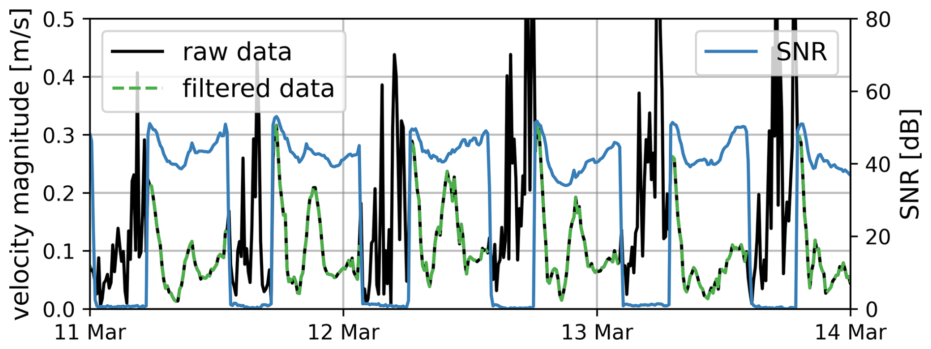
Figure 10 Example of filtering out low-water periods, during which the instrument was not submerged, from raw ADV velocity data at station B3, based on the instrument's signal-to-noise ratio (SNR).

The ADV velocity measurements are converted from XYZ to ENU coordinates by rotating the reference frame, using instrument orientations measured in the field with DGPS. The raw ADCP data are already in ENU coordinates, owing to the instruments' internal compasses, but a correction for the Earth's magnetic declination is applied because true north slightly differs from magnetic north: 2.6° for the Winter 2023–2024 campaign and 2.8° for the Spring 2025 campaign.

4.3 Wave spectral statistics

Wave spectral statistics are included in the tailored dataset and were derived per burst from ADV measurements using linear wave theory. Sea-surface elevation was reconstructed from near-bed pressure recordings following the approach of Van Der Lugt et al. (2024), which accounts for short-crested wind sea waves. The variance density spectrum of the sea surface was determined according to:

$$\begin{array}{}\text{(4)}& {\displaystyle }{P}_{\mathrm{SS}}=S_{\mathrm{W}}^{\mathrm{2}}{P}_{\mathrm{hydrostatic}}\text{(5)}& {\displaystyle }{S}_{\mathrm{W}}={\displaystyle \frac{\cosh \left(kd\right)}{\cosh \left(kh\right)}}\end{array}$$

with P_SS the variance density spectrum of the sea surface, P_hydrostatic the variance density of the hydrostatic surface elevation, k the wave number, d the local water depth, and h the instrument height above the bed. Sea-surface reconstruction was performed over the frequency band 0.125–1 Hz, which encompasses the short-crested wind sea waves observed at the measurement site, with peak frequencies up to 0.5 Hz. Energy at frequencies below 0.125 Hz is negligibly small at our measurement site and therefore omitted. To limit amplification of high-frequency noise within the integration range in the power spectrum, the linear transfer function S_W was capped at a maximum value of 5 and tapers to zero between 1 and 1.5 Hz. Further details on the sea-surface reconstruction method are provided by Van Der Lugt et al. (2024).

The spectral analysis yields the significant wave height $H_{m\mathrm{0}}=\mathrm{4}\sqrt{m\mathrm{0}}$, three mean wave periods $T_{m-\mathrm{1},\mathrm{0}}=\frac{m_{-\mathrm{1}}}{m_{\mathrm{0}}}$, $T_{m\mathrm{0},\mathrm{1}}=\frac{m_{\mathrm{0}}}{m_{\mathrm{1}}}$, and $T_{m\mathrm{0},\mathrm{2}}=\sqrt{\frac{m_{\mathrm{0}}}{m_{\mathrm{2}}}}$, the peak wave period T_p, and the smoothed peak wave period T_ps. The mean wave direction θ_mean (and directional spreading σ_θ) are determined following the method of maximum entropy (Lygre and Krogstad, 1986). All wave statistics are included in the tailored dataset.

4.4 Sediment transport and bed level measurements

Instrument-specific calibration curves (see Sect. 3.5) are used to convert the analogue signals of turbidity sensors into estimates of suspended sediment concentrations (SSC). To ensure values remain within each sensor's reliable operating range, SSC derived from Seapoint STMs is capped at 4000 mg L⁻¹, whereas SSC from the other turbidity sensors is capped at 8000 mg L⁻¹, corresponding to the upper limit of the calibration data. Periods during which turbidity instruments were exposed above the surface are excluded, consistent with the filtering applied to velocity measurements at the same height above the bed. No further filtering or despiking is applied. Suspended sediment transport rates are calculated by multiplying SSC with the corresponding flow velocities (i.e., [m s⁻¹] ⋅ [kg m⁻³] = [kg m⁻² s⁻¹]).

ADV and A-SED acoustic measurements of the instrument-to-bed distance are combined with instrument elevations obtained from DGPS measurements to produce time series of the local bed level, referenced either to NAP or to the bed level at deployment.

5 Supplementary data

The analysis and interpretation of this dataset can be complemented by several supplementary open datasets obtained through regular monitoring programs in the Dutch Wadden Sea, which are described below.

Rijkswaterstaat (the Dutch Ministry of Infrastructure and Water Management) maintains a network of permanent water level stations and wave buoys. Historical data from these stations are available upon request via https://waterinfo.rws.nl/ (last access: 17 June 2026). In addition, Rijkswaterstaat monitors suspended sediment concentrations through monthly to bimonthly water sampling, as part of its long-term water quality monitoring program. Measurement are available from over 50 stations dating back to 1973; however, at present only 10 stations located in or near the Dutch Wadden Sea are actively maintained (Stolte et al., 2023). The data can be requested via an online form (https://www.rijkswaterstaat.nl/formulieren/contactformulier-servicedesk-data, last access: 17 June 2026). Bathymetric surveys are conducted by Rijkswaterstaat at six-year intervals; the datasets can be requested via the same form as the sampling data. Data and models of the shallow and deep geology of the Netherlands are collected in the DINO database by the Geological Survey of the Netherlands, available through https://www.dinoloket.nl/ (last access: 17 June 2026). Hourly meteorological data can be accessed through the database of the Royal Netherlands Meteorological Institute (https://www.knmi.nl/nederland-nu/klimatologie/uurgegevens, last access: 17 June 2026; KNMI, 2026). The composition of the sediment bed is monitored as part of the SIBES (intertidal) and SUBES (subtidal) benthic survey programs coordinated by the Royal Netherlands Institute for Sea Research (NIOZ). The SIBES dataset is published by Bijleveld et al. (2025), whereas the SUBES dataset is not yet publicly available. The development of salt marshes in the Dutch Wadden Sea is regularly monitored by Wageningen Marine Research (WMR) using sedimentation-erosion bars (Elschot et al., 2020).

6 Applicability and limitations

6.1 Potential applications

The dataset enables quantitative analysis of flow and sediment transport under varying forcing conditions by tides, wind, and waves. This section illustrates the dataset content and its potential applications using data samples of measured current velocities, and bed elevation dynamics and SSC. Only a subset of the measurement locations is highlighted here; similar data are available for the other measurement locations.

6.1.1 Flow variability near the tidal divide

Tidal flows from two neighboring inlets (i.e., the Ameland Inlet to the west and the Friesche Zeegat to the east of the measurement site) are expected to meet at the (bathymetric) tidal divide. However, our field observations show that the location of hydrodynamic convergence varies considerably over time. This is illustrated in Fig. 11, which presents the ADCP (Aquadopp Profiler) measurements at locations A1, A3, and A5 during the Winter 2023–2024 campaign. Despite the measurement locations being close to the tidal divide, peak flood and ebb velocities reach 0.4–0.5 m s⁻¹. During flood tide, flow velocities at A1 are predominantly directed southeastward, whereas at A3 and A5 they are directed towards the southwest, indicating that A1 is located west of the tidal divide, while A3 and A5 are located east of the tidal divide. The ebb flow is generally directed in opposite direction of the flood flow. During certain tidal periods, however, flood currents at A1 are directed southwestward instead of southeastward, and ebb currents are directed eastward, indicating exchange through the eastern inlet and a temporarily varying location of the tidal divide depending on the wind conditions.

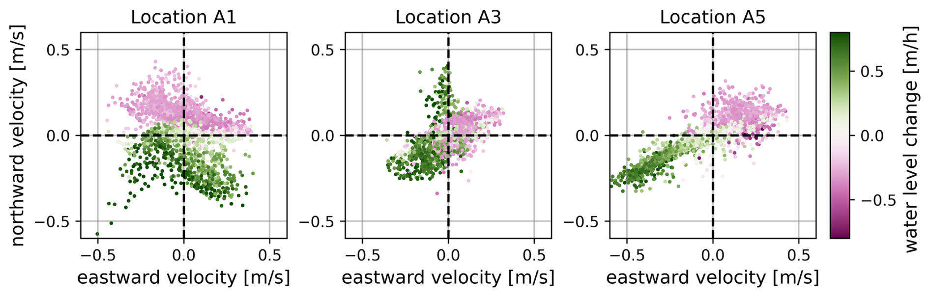
Figure 11 Depth-averaged flow velocities (ADCP measurements) at stations A1, A3, and A5 during the Winter 2023–2024 campaign, with the tidal phase represented by the change in water level.

6.1.2 Local sediment resuspension on mudflats

In the first days of the Spring 2025 campaign, until 11 February, the fringing mudflat eroded several centimeters, leading to a temporary increase in local SSC. This is illustrated in Fig. 12, which presents time series of bed elevation (distance to bed measurements with an ADV instrument) and SSC (STM measurements) at station B3. The bed elevation on the mudflat, although dynamic during individual tidal cycles, recovered under calm conditions in subsequent weeks and remained relatively stable during late February and early March, with SSC minima observed during neap tides (around 23 February and 9 March). In the latter half of March, bed elevation dynamics intensified, as moderate wave activity induced resuspension, bed erosion, and elevated SSC. These erosional events were typically followed by rapid recovery of the bed elevation during intermittent calm periods.

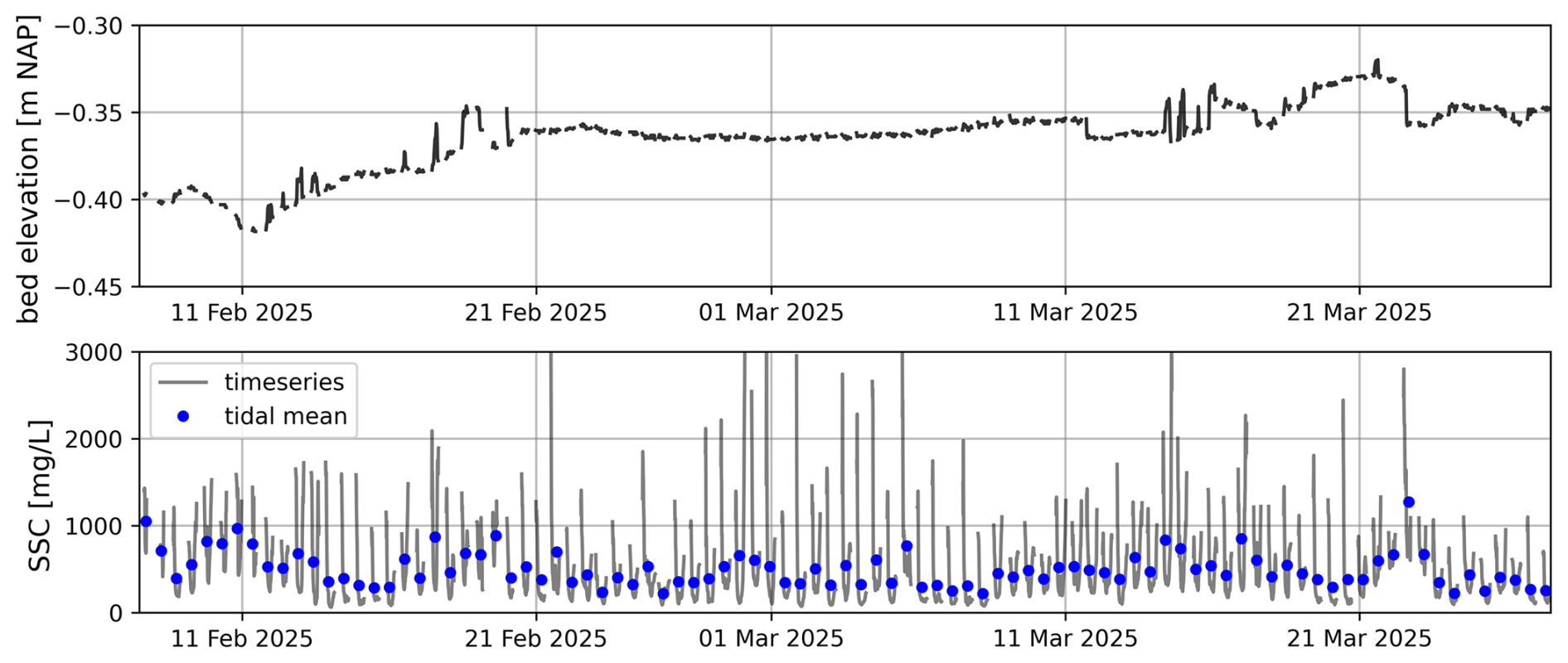
Figure 12 Time series of bed elevation (top; ADV bottom check) and SSC (bottom; STM turbidity measurements) at station B3 during the Spring 2025 campaign. Data gaps correspond to instrument emergence during low water.

6.2 Limitations

Limitations of the measurement data originate from instrument accuracy, turbidity sensor calibration, and data processing. The accuracy of high-frequent acoustic flow velocity measurements (bias <1 % of the measured velocity; Nortek AS, 2018) is considered negligible for typical applications in coastal and estuarine systems. Turbidity sensors have an upper operating limit due to signal saturation (Fettweis et al., 2019), but this limit was not reached during the field measurements. The main source of uncertainty in SSC timeseries follows from changes in the suspended sediment composition over time. The relationship between turbidity and SSC (Sect. 3.5) is sensitive to the sediment characteristics, as particles of different sizes, shapes, and mineral compositions scatter light differently (Downing, 2006). Optical turbidity sensors were calibrated with one type of sediment mixture. Therefore, the calibration does not reflect temporal changes and spatial variations in suspended sediment composition. Resulting SSC values (in mg L⁻¹) may therefore deviate from the actual concentrations. Changes in sediment composition may be estimated from acoustic and optic instruments deployed in parallel (Pearson et al., 2021; Lin et al., 2020), but such an analysis has not been performed yet.

Wave spectral statistics are derived from near-bed pressure recordings, using a wave attenuation correction factor (S_W in Sect. 4.3) to reconstruct the short-crested wind sea waves. A cap on the correction factor prevents blow-up of noise, but also underestimates the variance density of high-frequency waves. Wave spectral statistics are therefore unreliable when high-frequency waves (>1 Hz) are dominant. Such conditions occurred frequently during the calm weather periods in the Spring 2025 campaign.

7 Code and data availability

The data collected during the two field campaigns presented in this article have been published as a collection of three datasets at 4TU Centre for Research Data (https://doi.org/10.4121/bbb85feb-15f9-476f-9598-b6509392117d; van Weerdenburg et al. (2026)). The first and second datasets contain the in situ measurements from the Winter 2023–2024 and Spring 2025 field campaigns, respectively. The third dataset contains sediment bed composition data of samples collected during both campaigns.

The in situ measurements are provided in NetCDF format and are organised into raw data (folder 01_RawData), filtered data (folder 02_ProcessedData), and tailored data (folder 03_TailoredData; see Sect. 4 for details). NetCDF files are also made available through the 4TU OPeNDAP data service. Python scripts used to convert the raw data into filtered and tailored datasets are available in folder 04_Processing. Sediment data obtained from the different laboratory analyses (see Sect. 3.4) are provided in Excel sheets.

8 Summary and outlook

The presented dataset on hydrodynamics, sediment transport, and bed level dynamics was collected during two dedicated measurement campaigns in the Dutch Wadden Sea. Multiple storms are captured during the first (Winter 2023–2024) campaign, including one with exceptionally high water level set-up on 21 December 2023. The strong wind forcing during this measurement period allows for a quantitative analysis of the relative importance of wind- and tide-driven flow and transport. Measurement sites in this campaign were predominantly sandy. In addition to the sediment exchange between tidal basins, the second measurement campaign in Spring 2025 also focused on the sediment exchange with, and the morphological development of, a fringing mudflat. Weather conditions during this measurement period were relatively calm, resulting in net accretion at intertidal mudflat locations and predominantly tide-driven transport.

Data from the various instruments have been processed in a consistent and reproducible manner and are available at multiple levels of detail to encourage reuse by the broader scientific community and to advance our understanding of sediment dynamics in tidal systems like the Dutch Wadden Sea. Specifically, the dataset is intended to support quantitative analyses of sediment exchange between tidal divides, as well as between channels and shoals.