PolyU2025 SLA: a global 0.25°  ×  0.25° monthly sea-level anomaly dataset (1993–2024) determined from satellite altimetry for sea-level and climate change research

Long-term and spatially consistent sea-level anomaly (SLA) products derived from satellite altimetry are fundamental for sea-level and climate change studies. In this study, we develop the PolyU2025 SLA (The Hong Kong Polytechnic University 2025 sea-level anomaly), a new global monthly gridded SLA product generated using a fully independent data-processing framework. This product is provided on a regular 0.25°×0.25° grid and spans the period from January 1993 to December 2024 and is intended to be updated regularly. The PolyU2025 SLA is evaluated through systematic intercomparisons with the Copernicus Climate Change Service (C3S) gridded SLA product as well as with independent tide gauge observations. The results demonstrate a high level of consistency between PolyU2025 and C3S at global and basin scales, characterized by near-zero differences in global-mean SLA and statistically indistinguishable estimates of global mean sea-level trends and accelerations, indicating that both products are suitable for long-term sea-level change studies. At regional and short time scales, differences between the two products become more pronounced, particularly in dynamically active regions, and are mainly associated with differences in the representation of short-term and mesoscale variability. These differences reflect methodological trade-offs in data processing and spatial mapping rather than systematic biases. Overall, the PolyU2025 SLA provides a robust and consistent characterization of sea-level change from regional to global scales and serves as a complementary dataset to existing gridded SLA products, especially for long-term and climate-oriented sea-level studies and multi-product assessments of regional sea-level variability and uncertainty. The PolyU2025 SLA product is openly available at https://doi.org/10.5281/zenodo.17810525 (Yuan et al., 2025).

1 Introduction

Sea-level is one of the key indicators of global climate change. It represents the integrated effects of energy accumulation and mass redistribution within the climate system (IPCC, 2023), reflecting the combined influence of fundamental processes including ocean thermal expansion (Liang et al., 2025), land ice mass loss (Nie et al., 2024, 2025), and changes in terrestrial water storage (Chandanpurkar et al., 2025). In the context of ongoing global warming, global mean sea-level (GMSL) has continued to increase, with a pronounced acceleration in its rate of rise in recent decades (Hamlington et al., 2024; Mu et al., 2025a; Nie et al., 2025). Based on global tide gauge (TG) reconstructions, GMSL has risen by roughly ∼100 mm since the early 1990s (Mu et al., 2025a). Using high-precision satellite radar altimetry, which has provided consistent global sea surface height (SSH) measurements since 1993, GMSL is estimated to have increased by approximately 111 mm by the end of 2023 (Hamlington et al., 2024). Moreover, the rate of sea-level rise has nearly doubled, from about 2.1 mm yr⁻¹ in 1993 to approximately 4.5 mm yr⁻¹ in 2023 (Hamlington et al., 2024). This ongoing rise in sea-level poses significant challenges to socioeconomic development and coastal sustainability worldwide, with particularly critical implications for low-lying coastal zones and densely populated coastal cities (Adebisi et al., 2021).

At present, sea-level change is primarily observed using two complementary systems: TGs and satellite radar altimeters. TGs provide long-term, high-temporal-resolution records of sea-level at specific coastal locations, which are an essential data source for investigating global, regional and local sea-level variability. However, their spatial coverage is highly uneven, and their measurements often lack a unified geocentric vertical reference frame. Additionally, TG records are influenced by non-oceanic signals such as vertical land motion (Vignudelli et al., 2011; Cipollini et al., 2017; Peng et al., 2024), which complicates the interpretation of sea-level trends. As a result, in the absence of independent constraints, TG observations alone are insufficient for accurately assessing global sea-level change. In contrast, satellite radar altimetry has revolutionized sea-level monitoring since the early 1990s by providing continuous, high-precision SSH measurements with near-global coverage. Advances in technology and rigorous cross-calibration between satellite missions have resulted in a more than 30-year-long, globally consistent record of sea-level change in a unified geocentric reference frame. This enables quantification of both global and regional sea-level trends with high accuracy (Meyssignac et al., 2023; Guérou et al., 2023; He et al., 2024). Satellite altimetry is now central to sea-level research, offering comprehensive data that support climate studies, coastal management, and policymaking (Cazenave and Moreira, 2022; Hamlington et al., 2024; Mu et al., 2025a).

Despite the high precision and strong physical consistency of along-track satellite altimetry observations, their spatial and temporal sampling is inherently non-uniform due to limitations imposed by orbital configurations and repeat cycles (Martin et al., 2023). This non-uniform sampling of along-track observations prevents them from directly meeting the requirements of long-term sea-level change studies. Specifically, along-track measurements alone do not provide SSH fields that are temporally continuous and spatially consistent. To address this, researchers commonly integrate multi-mission along-track sea-level anomalies (SLAs) in a unified reference frame and apply spatiotemporal mapping techniques to generate regularly gridded SLA fields. This approach has become standard practice for global and regional sea-level monitoring and related climate research (Guérou et al., 2023; Sánchez-Román et al., 2023).

Currently, the most widely used gridded SLA products are produced by the Data Unification and Altimeter Combination System (DUACS) and distributed as successive delayed-time (DT) reprocessed datasets. Since the DT2010 (Dibarboure et al., 2011) release, DUACS has continuously improved its global gridded SLA product through subsequent versions such as DT2014 (Pujol et al., 2016), DT2018 (Taburet et al., 2019), DT2021 (Sánchez-Román et al., 2023), and the most recent DT2024 (Ballarotta et al., 2025). These updates incorporated new altimeter missions, refined processing standards, and enhanced spatiotemporal mapping strategies to adapt to the evolving sampling characteristics of the altimeter satellite constellation (Pujol et al., 2016; Taburet et al., 2019; Sánchez-Román et al., 2023; Ballarotta et al., 2025).

Within the DUACS framework, two main categories of gridded SLA products are provided to meet different scientific needs (Taburet et al., 2019; Sánchez-Román et al., 2023). The first category, all-satellites products, use all available satellite data at any given time to maximize the spatiotemporal sampling and improve the representation of mesoscale and higher-frequency oceanic signals. The second category, two-satellite products, is based on a fixed dual-satellite configuration, ensuring stable geometry and error characteristics over the entire time series. This temporal stability makes two-satellites products are particularly suitable for estimating long-term sea-level trends and accelerations at both global and regional scales.

However, for long-term sea-level change studies, only a limited number of gridded SLA products are optimized to accurately represent long-term trends and low-frequency sea-level variability. The main reference products are those released under the Copernicus Climate Change Service (C3S) framework, which are based on the DUACS. Previous studies have shown that the construction of gridded SLA fields is highly sensitive to the selection of input altimeter missions, the methods used to ensure inter-mission consistency, and the adopted spatiotemporal mapping strategies (Dibarboure et al., 2011; Pujol et al., 2016; Taburet et al., 2019; Sánchez-Román et al., 2023; Ballarotta et al., 2025). These processing choices often involve trade-offs between resolving mesoscale variability and ensuring long-term stability, leading to spatially heterogeneous differences in the resulting products. Such differences are especially pronounced in coastal regions and areas with high oceanic variability, where different DUACS product types and reprocessing versions have shown varying performance characteristics (Pujol et al., 2016; Taburet et al., 2019; Sánchez-Román et al., 2023).

Given these challenges, developing complementary gridded SLA datasets using independent data-selection schemes and processing strategies is crucial. Such efforts help assess the robustness of existing mainstream products in long-term sea-level change studies, improve the understanding of how methodological differences affect estimates of long-term sea-level change, and provide multi-source benchmark datasets for cross-validation in global and regional sea-level research. In this study, we present a new global monthly gridded SLA product, termed PolyU2025 SLA (The Hong Kong Polytechnic University 2025 sea-level anomaly; hereafter PolyU), along with a comprehensive evaluation of its performance. The PolyU dataset is constructed using an independent data-processing and mapping framework. It offers a spatial resolution of 0.25°×0.25°, and covers the period from January 1993 to December 2024, with plans for continuous updates.

The remainder of this paper is organized as follows. Section 2 describes the satellite altimetry and auxiliary datasets used in this study. Section 3 presents the methodology for constructing the monthly gridded SLA product. Section 4 compares PolyU with the C3S gridded SLA product. Section 5 evaluates PolyU against independent TG observations. Section 6 provides information on data availability. Finally, Sect. 7 discusses the results and presents the main conclusions.

2 Data

2.1 Altimetry data

The satellite altimetry data used in this study are obtained from along-track Level-2P (L2P) products released by the Archiving, Validation and Interpretation of Satellite Oceanographic Data (AVISO, https://www.aviso.altimetry.fr/, last access: 24 December 2025). These L2P products are generated by the 1 Hz mono-mission processing chains for each satellite mission, including Sentinel-6A, Sentinel-3A/B, CryoSat-2, SARAL/AltiKa, HaiYang-2A/B, Jason-1/2/3, Geosat Follow-On (GFO), ERS-1/2, Envisat, and TOPEX/Poseidon (T/P). The L2P datasets provide geophysically corrected SSH measurements as the primary observable, as well as the derived SLA variable computed relative to a mean sea surface (MSS).

All L2P products are referenced to the WGS84 ellipsoid and processed using the standardized geophysical correction framework described in Kocha et al. (2023). This includes corrections for wet and dry tropospheric effects, ionospheric delay, ocean and solid earth tides, sea-state bias, and dynamic atmospheric effects. The SLA values are derived with reference to the Hybrid2023 MSS model (Laloue et al., 2025), which combines three recent MSS models, CNES_CLS22 (Schaeffer et al., 2023), SCRIPPS_CLS22 (Sandwell, 2024) and DTU21 (Andersen et al., 2023), to improve accuracy in both open-ocean and coastal regions.

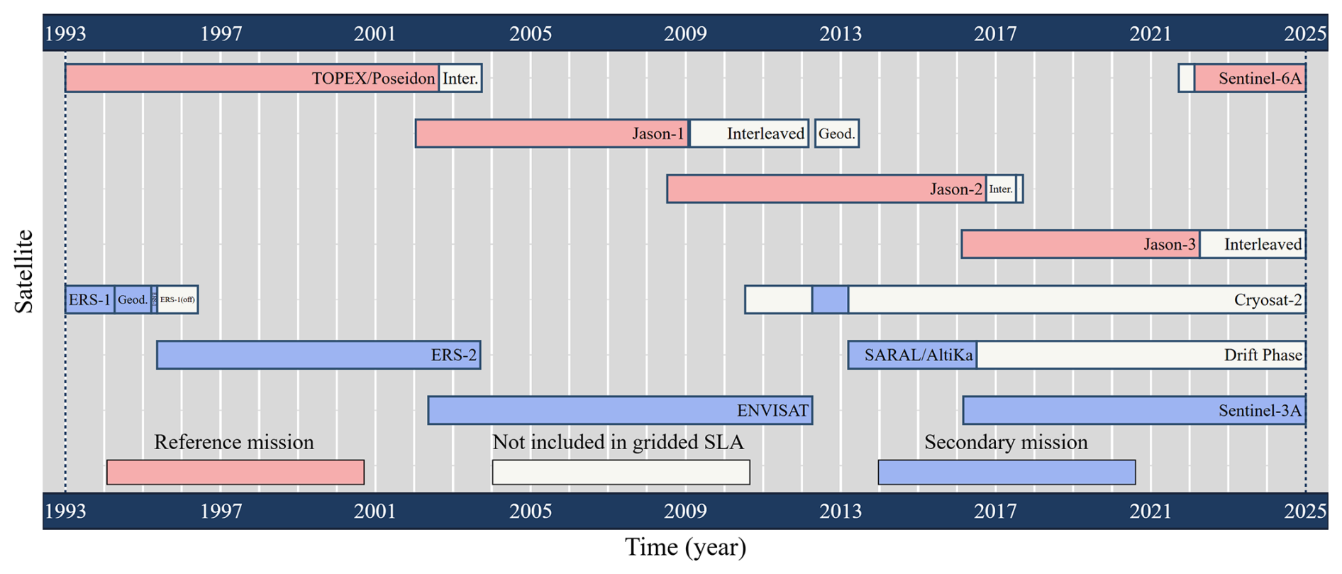
For this study, eleven satellite altimetry missions were selected (Fig. 1). These include the primary reference missions (T/P, the Jason series, and Sentinel-6A), which ensure long-term temporal continuity, and the secondary missions (CryoSat-2, SARAL/AltiKa, ERS-1/2, Envisat, and Sentinel-3A), which enhance spatial coverage. Collectively, these missions provide continuous global ocean observations spanning the entire altimetric era from January 1993 to December 2024.

Figure 1 Overview of the SLA product availability period from each altimetric mission.

To generate a climate-consistent monthly gridded SLA product, a minimum of two concurrent altimetry missions were adopted for each month of the study period. This approach is consistent with previous multi-mission altimetry studies (Pujol et al., 2016; Taburet et al., 2019; Sánchez-Román et al., 2023; Ballarotta et al., 2025), which have demonstrated that maintaining a stable two-satellite configuration is essential for effective inter-mission cross-calibration, temporal consistency across the altimetric record, and long-term stability of mean sea-level estimates.

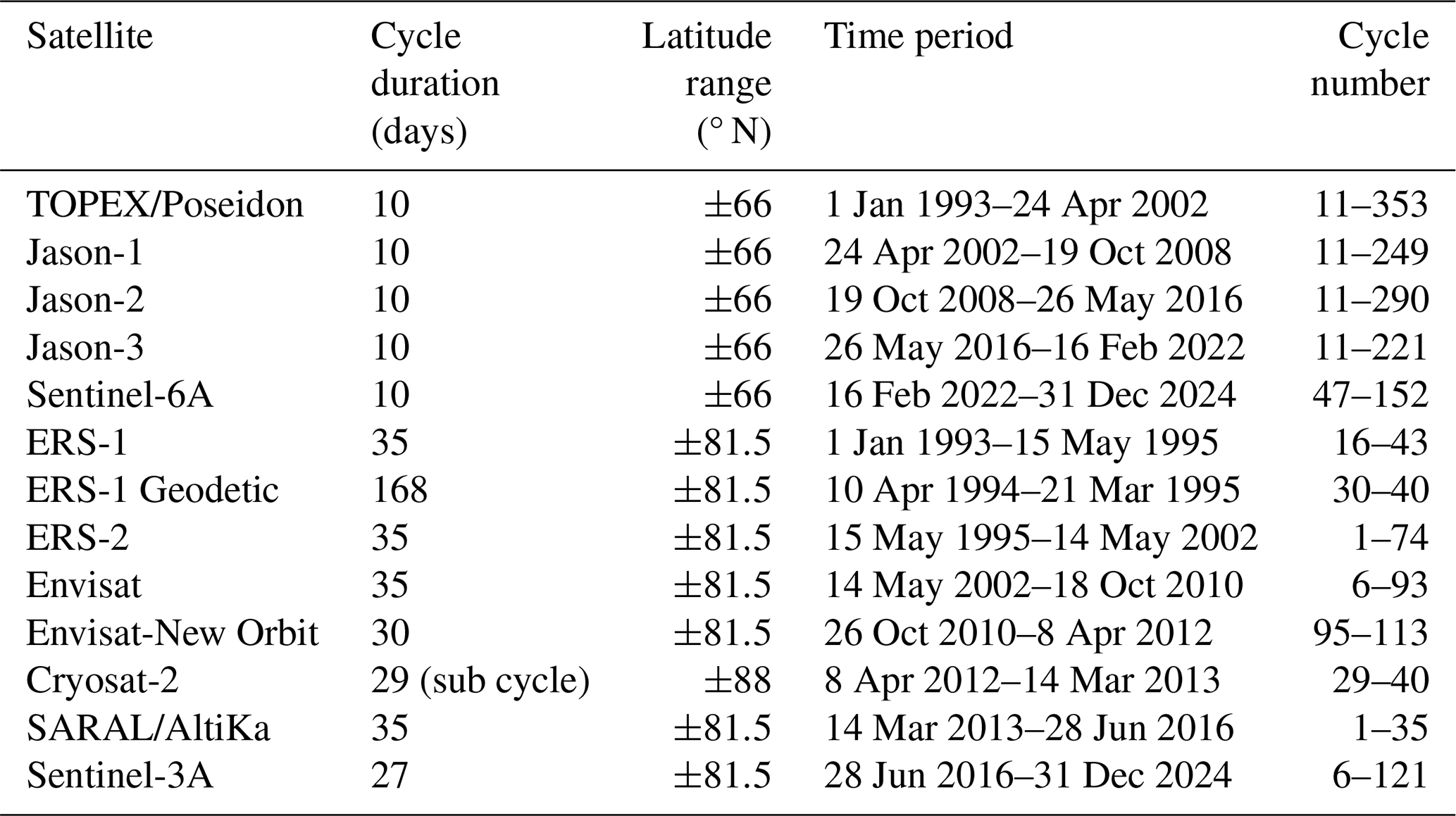
The characteristics of the selected missions, including temporal coverage, repeat cycles, latitude range and cycle numbers, are summarized in Table 1. This configuration ensures that at least two altimetry missions contribute data in every month from January 1993 to December 2024, with the sole exception of the period from January and March 1994, when T/P was the only operating mission and thus the exclusive source of SLA observations.

Table 1 Characteristics and time availability of the satellite altimetry missions used in this study.

2.2 Copernicus C3S gridded sea-level product

The gridded sea-level dataset used for validation in this study is the C3S Global Ocean Level-4 SLA product (hereafter referred to as C3S), produced by Collecte Localisation Satellites (CLS) and publicly available through the Copernicus Climate Data Store (Product DOI: https://doi.org/10.48670/moi-00145, E.U. Copernicus Marine Service Information, 2024). The C3S dataset provides global coverage on a 0.25°×0.25° grid and currently spans the period from January 1993 to May 2025. It is routinely updated in delayed mode, with an approximate latency of five months. Both daily and monthly gridded products are distributed in NetCDF-4 format.

The daily SLA fields are produced using the DUACS delayed-time processing chain (Pujol et al., 2016; Taburet et al., 2019; Sánchez-Román et al., 2023; Ballarotta et al., 2025), which includes Level-2 quality control, inter-mission cross-calibration, orbit error removal, bias correction and an optimal interpolation (OI) mapping step. Monthly SLA fields are subsequently obtained by computing the arithmetic mean of the validated daily maps for each calendar month.

2.3 Tide gauge observations

The TG observations used for comparison with satellite altimetry were obtained from the Permanent Service for Mean Sea Level (PSMSL; https://psmsl.org/, last access: 24 December 2025), which provides globally distributed TG observations in standardized formats with long-term quality control (Holgate et al., 2013). To ensure statistical significance and stable trend estimation, only TG stations with at least 10 years of observational data between January 1993 and December 2024 were included in the analysis (Ablain et al., 2019; Ramos-Alcántara et al., 2022). Prior to further analysis, monthly values exceeding three times the standard deviation of each time series were removed, as such extremes are likely associated with localized effects (e.g., river discharge) rather than large-scale oceanic sea-level variability (Laíz et al., 2013). After this quality-control procedure, only stations retaining 90 %–100 % of valid monthly data were preserved, resulting in a final dataset of 889 stations. This dataset serves as a comprehensive reference for evaluating the performance of gridded SLA products across a wide range of coastal and near-coastal environments.

To ensure consistency with the altimetry-derived SLA fields, TG observations were corrected for dynamic atmospheric effects. In satellite altimetry processing, the dynamic atmospheric correction (DAC), which accounts for low-frequency inverse barometer responses and high-frequency wind- and pressure-driven forcing, is removed to isolate the oceanic sea-level signal (Carrère and Lyard, 2003). Accordingly, the same DAC product used in the altimetry processing was applied to the TG observations. The DAC fields, provided at 6 h temporal resolution and 0.25° spatial sampling by the AVISO, were extracted at the nearest grid point to each station and averaged to monthly means. These monthly DAC values are then subtracted from the TG records to obtain the oceanic component of sea-level variability.

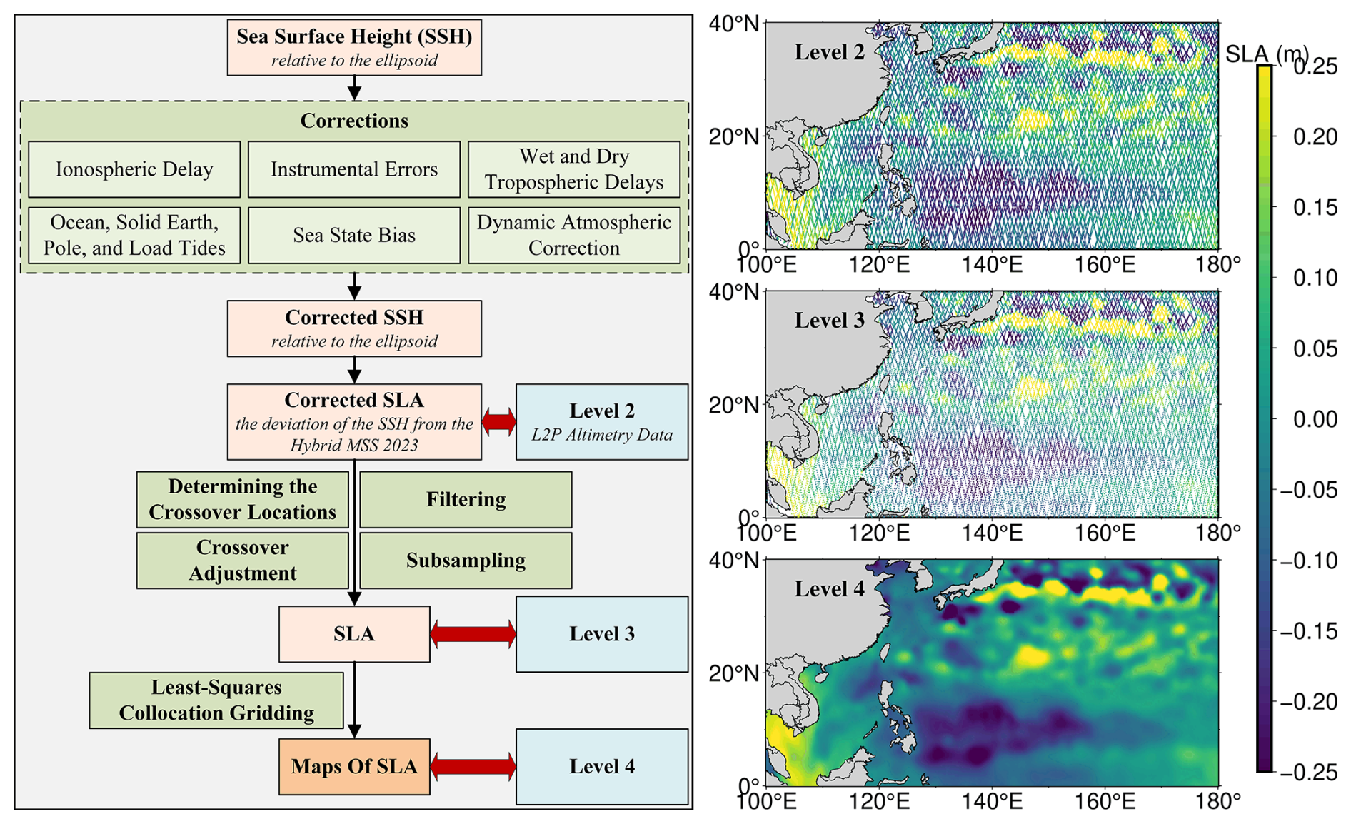
Figure 2 Overview of data processing steps and evolution of satellite altimetry data from Level 2 to Level 4.

3 Methodology

Figure 2 presents the complete processing workflow and representative examples at each processing stage. The left panel outlines the steps from the initial along-track L2P altimetry data to the final Level 4 gridded SLA product. The workflow begins with L2P products, which have already corrected for instrumental and geophysical effects. The SLA is first extracted along each satellite ground track. Next, crossover locations are identified for each satellite mission individually (self-crossovers) as well as between different satellite tracks (ascending–descending, ascending–ascending or descending–descending intersections). Crossover adjustments are then applied to both mono-mission and inter-mission crossovers to mitigate residual orbit errors and reduce discrepancies between tracks. After crossover corrections, the SLA records are filtered to suppress high-frequency variability that cannot be reliably reconstructed from the along-track sampling. The data are then spatially subsampled to be commensurate with the filtering, so that only as many points as needed to represent the remaining spectral content are retained, and the sampling density across missions is standardized prior to the gridding step (Pujol et al., 2016; Taburet et al., 2019). These processed observations constitute the Level 3 dataset. To generate the final gridded product, a least-squares collocation (LSC) method is applied to the irregularly distributed Level 3 data. This approach produces spatially optimal SLA estimates on a regular 0.25°×0.25° grid, while accounting for the spatial covariance structure of the SLA field.

The right panel of Fig. 2 provides representative examples of each processing level. At Level 2, the dense along-track SLA data contain noticeable noise; At Level 3, the data show improved internal consistency after crossover adjustment, filtering and subsampling. Finally, Level 4 displays the gridded SLA product, which is suitable for long-term sea-level change studies due to its improved spatial consistency and reduced noise. Detailed descriptions of the crossover identification, adjustment, filtering, subsampling, and LSC gridding procedures are provided in the subsequent sections.

3.1 Crossover point identification

A crossover point is the location where two satellite ground intersect, either from different passes of the same mission or from different satellite missions. At each crossover, two independent SSH measurements can be obtained: one from each crossing track. The difference between these measurements, referred to as the crossover difference, captures the combined effects of orbit errors, residual geophysical correction errors, measurement noise, and other systematic effects. These crossover differences provide an effective diagnostic for estimating orbit and height-bias corrections, thereby improving the internal consistency of altimetry observations both within individual missions and across multiple missions.

To obtain SSH values at each crossover, cubic-spline interpolation is applied to the neighboring along-track observations that bracket the crossover point. Measurement time and other ancillary parameters are determined using linear interpolation. This combination of interpolation schemes is employed because SSH is particularly sensitive to observational noise and along-track variations in ocean surface topography, while temporal and ancillary variables tend to vary more smoothly. To reduce contamination from true ocean variability, the temporal separation between two SSH measurements at a crossover is restricted to less than 10 d.

3.2 Crossover adjustment

Crossover differences arise from multiple error sources, as described in Sect. 3.1. Traditional crossover adjustment methods typically assume that orbit error is the primary contributor and focus on mitigating orbit-related effects. However, advances in altimetry correction theory and improvements in geophysical corrections have significantly enhanced the overall quality of altimetric measurements. At the same time, progress in precise orbit determination and orbit modeling has greatly reduced orbit error. As a result, orbit error is no longer the dominant source of crossover difference; its magnitude is now comparable to other error sources, such as residual geophysical-correction errors, measurement noise, and remaining systematic effects. Therefore, crossover differences should be interpreted as the combined influence of multiple error sources and crossover adjustment must account for the combined contributions of all major error sources.

To better represent the combined influence of multiple error sources while maintaining a streamlined workflow and ensuring stable and reliable solutions, Huang et al. (2008) introduced a modified crossover adjustment procedure. This method is carried out in two stages: (i) applying a condition adjustment model to the crossover observation equations, and (ii) filtering and predicting observational corrections along each track using an appropriate error model. Further details of this approach can be found in Huang et al. (2008), with methodological refinements introduced in later studies by Yuan et al. (2020, 2021, 2023).

The combined effect of crossover-related errors exhibits complex temporal variability, including both linear and periodic components, as well as mixed behaviours from their interaction. To capture this, a hybrid polynomial model with observational time as the independent variable is used to represent the crossover error term (Huang et al., 2008):

$$\begin{array}{}\text{(1)}& \begin{array}{rl}f\left(T\right)& =A_{\mathrm{0}}+A_{\mathrm{1}}\cdot \left(T-T_{\mathrm{0}}\right)+\sum _{i=\mathrm{1}}^M\left(B_i\cdot \cos \left(i\cdot \mathit{\omega }\cdot \left(T-T_{\mathrm{star}}\right)\right)\right.\\ & \left.+C_i\cdot \sin \left(i\cdot \mathit{\omega }\cdot \left(T-T_{\mathrm{star}}\right)\right)\right),\end{array}\end{array}$$

where T is the observation time; A₀, A₁, B_i, $C_i(i=\mathrm{1},\mathrm{\cdots },M)$ are model parameters to be estimated; ω represents the angular frequency corresponding to the duration of a surveying track ($\mathit{\omega }=\mathrm{2}\mathit{\pi }/(T_{\mathrm{end}}-T_{\mathrm{star}})$, where T_star and T_end are the start and end times of the surveying track, respectively); and M is a positive integer determined by the length of the track. Empirically, M is set to 1–2 for a short track, 3–5 for a medium-long track, and 6–8 for a long track.

To improve the internal consistency of multi-mission altimetry observations, crossover adjustment was applied before generating the gridded SLA fields. The datasets listed in Table 1 were divided into monthly segments from January 1993 to December 2024, and an independent self-crossover adjustment was performed for each satellite mission within every month. Figure 3 presents the standard deviation (SD) of crossover differences before (Fig. 3a) and after (Fig. 3b) self-crossover adjustment for all missions across all monthly segments. This adjustment substantially reduces the SD of crossover differences for every mission, indicating a marked improvement in internal consistency and data reliability.

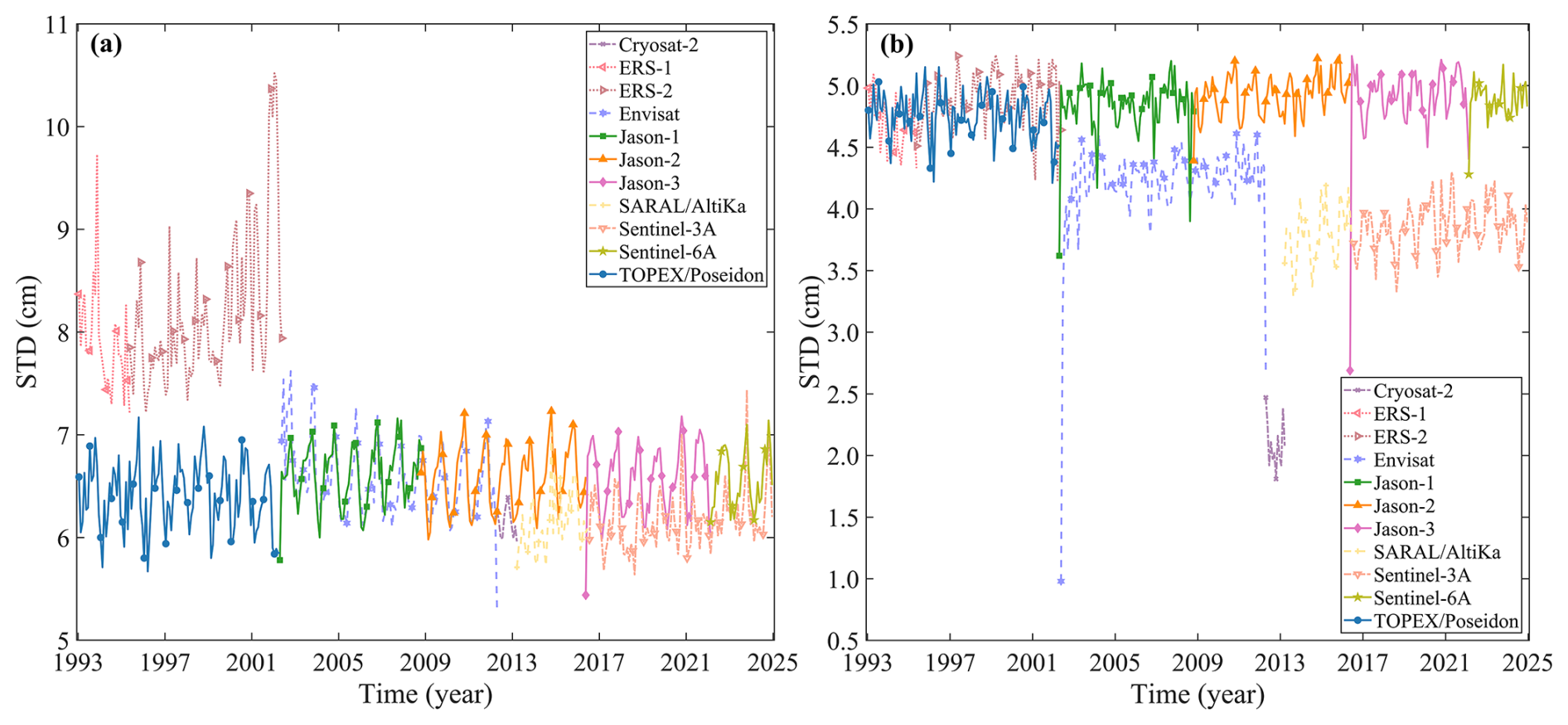
Figure 3 SD of crossover differences for individual altimetry missions before (a) and after (b) crossover adjustment.

Among all missions, CryoSat-2 exhibits the greatest improvement, with its monthly mean SD reduced from 6.15 to 2.09 cm, corresponding to an enhancement of approximately 66 %. ERS-1, ERS-2, Sentinel-3A, SARAL/AltiKa, and Envisat also show notable reductions of about 35 %–40 %. In contrast, T/P, the Jason series (Jason-1/2/3), and Sentinel-6A display more moderate reductions of approximately 25 %–27 %. These results demonstrate that crossover adjustment enhances the quality and internal consistency of satellite altimetry data by constraining orbit-related errors and statistically reducing the influence of measurement noise and local anomalies on along-track observations. The improvement tends to be more pronounced for earlier missions or those with relatively higher noise levels, whereas reference missions with inherently high accuracy exhibit more modest enhancements.

In the data processing workflow, an independent self-crossover adjustment is first applied to each satellite mission within every monthly segment to correct for mission-specific errors and improve internal consistency. Subsequently, for each month, crossover adjustments are performed between the secondary missions and the designated reference mission. At these inter-mission crossover locations, any remaining crossover differences are primarily attributed to measurement errors in the secondary mission, as the reference mission serves as the benchmark to ensure the long-term temporal stability of the entire SLA record.

While crossover adjustment remarkably improves the precision and internal consistency of the along-track observations, some residual errors inevitably persist due to factors such as unmodeled geophysical effects, instrument noise, and local anomalies. To account for these remaining uncertainties, the subsequent LSC gridding procedure (see Sect. 3.4) incorporates the post-adjustment standard deviation of single-satellite crossover differences as the noise level for each satellite dataset. This approach ensures that the LSC method appropriately weights the observations according to their estimated accuracy, thereby improving the reliability and robustness of the final gridded SLA product.

3.3 Filtering and subsampling

After crossover adjustment, the along-track SLA records are filtered and subsampled before gridding. This step is essential for suppressing high-frequency measurement noise and removing small-scale signals that cannot be reliably reconstructed due to the intrinsic along-track and cross-track sampling limitations of satellite altimetry (Ducet et al., 2000; Dufau et al., 2016; Pujol et al., 2016). A latitude-dependent linear Lanczos low-pass filter is applied, following principles used in the DUACS. The filter uses longer cut-off wavelengths in the tropics (≈200 km) and progressively shorter cut-offs at higher latitudes (down to about 65 km above 40°). This approach is consistent with the observed meridional decrease in mesoscale energy, where smaller-scale features become more prominent at higher latitudes (Dufau et al., 2016; Pujol et al., 2016). To ensure that the spatial sampling matches the filter-imposed resolution and to avoid redundant observations along the ground tracks, the filtered SLA data are then subsampled. Specifically, one point is retained for every seven along-track observations between 10° N and 10° S, one in five between 10 and 30° in both hemispheres, and one in three at latitudes above 30° (Ducet et al., 2000). This adaptive subsampling strategy ensures that the data density is consistent with the effective spatial resolution set by the filtering process. The combined filtering and subsampling step reduce noise, prevents oversampling from biasing the gridding solution, and produces a spatially homogeneous Level-3 dataset for the subsequent LSC gridding.

3.4 Least-squares collocation gridding

LSC a widely used and highly effective method for gridding satellite altimetry data (Jordan, 1972; Moritz, 1978; Rapp and Bašić, 1992; Jin et al., 2016; Yuan et al., 2020; 2023). LSC is particularly advantageous because it explicitly accounts for the spatial covariance structure of both the signal and the noise, providing optimal interpolation estimates at arbitrary grid locations. This makes it well suited for reconstructing SLA fields from irregularly distributed along-track observations (Jin et al., 2016). For LSC to achieve optimal performance, it is essential to accurately model the signal covariance, noise covariance, and the cross-covariance between the true signal and the observations. In this study, a two-dimensional, isotropic second-order Markov process is adopted to represent the spatial covariance function. This model provides the necessary prior statistical information for the altimetry observations and facilitates the construction of the covariance matrices, thereby improving the accuracy of the LSC-based gridding. The second-order Markov covariance function can be expressed as (Jordan, 1972; Moritz, 1978):

$$\begin{array}{}\text{(2)}& D\left(d\right)=D_{\mathrm{0}}\cdot (\mathrm{1}+d/\mathit{\alpha })\cdot e^{-d/\mathit{\alpha }},\end{array}$$

where d is the spherical distance between an observation and a grid point. D₀ represents the signal variance and describes the covariance amplitude at zero distance; it can be estimated from the sample variance of observations located around the grid point. α is the spatial correlation length, which controls the decay rate of the covariance with increasing distance. The value of α varies with latitude; it is typically 200–240 km in low latitudes, 100–120 km in mid-latitudes, and 60–100 km in high latitudes. In the LSC gridding interpolation process, the noise variance of observations is determined as the crossover difference accuracy after self-crossover adjustment, divided by $\sqrt{\mathrm{2}}$ for each satellite mission.

In the present study, LSC gridding was performed independently for each monthly SLA field using observations acquired within the corresponding month. Before gridding, multi-mission altimeter observations were adjusted through crossover analysis to reduce inter-mission and inter-track inconsistencies, as well as part of the mismatch associated with different observation times within the monthly sampling window. Since each monthly field was reconstructed independently and the temporal span of the input observations was limited, the residual temporal decorrelation effect was considered secondary relative to the spatial covariance structure. Therefore, a purely spatial covariance function was adopted in the current monthly gridding framework.

To ensure accurate and stable interpolation, it is important to use a sufficient number of observations that are spatially well-distributed around each grid point. In practice, a circular search window centered on the grid point is used, with an initial radius of about twice the grid spacing. At least 40 observations are required within this window to maintain the numerical stability of the covariance matrix. If the initial search window does not contain enough data, the radius is gradually increased until the minimum sample size is reached. Additionally, the search region is divided into eight quadrants, with each quadrant required to contain at least 5–10 observations. This approach prevents the data from being overly concentrated along the satellite-track direction and ensures a more uniform spatial sampling. Such a strategy is crucial for reducing anisotropy in the data distribution, which can otherwise bias the gridding solution and degrade the quality of the interpolated SLA fields. By carefully modeling the spatial covariance and ensuring robust local sampling, LSC provides high-quality, spatially consistent gridded SLA products that are well-suited for climate studies and oceanographic applications.

Given the considerable computational cost associated with LSC, a regional block-wise strategy is further implemented to enhance computational efficiency. Specifically, the domain from 8° S to 60° N is divided into 20°×20° blocks, while the region from 60 to 80° N is partitioned into 24°×20° blocks. This results in a total of 144 subregions, of which 141 contain valid SLA observations; the remaining three are located over continental land areas. LSC gridding is performed independently within each subregion, followed by a merging and integration step to reconstruct the global field. For grid lines located within overlapping areas between adjacent subregions, a weighted averaging scheme based on the associated error estimates is applied to ensure smooth transitions and spatial consistency. In this way, the proposed strategy significantly reduces computational demand while preserving the stability, continuity, and reliability of the final gridded results.

3.5 Methodological differences between PolyU and C3S gridded SLA products

Both the PolyU and C3S gridded SLA products are derived exclusively from satellite altimetry observations provided by L2P products (see Sect. 2.1), ensuring a consistent observational basis for intercomparison. To construct monthly SLA fields, both datasets require input from at least two concurrent satellite missions per month. This approach guarantees robust temporal continuity and comprehensive spatial coverage throughout the multi-decadal record (Pujol et al., 2016; Taburet et al., 2019; Sánchez-Román et al., 2023).

Despite these common foundations, the two products are generated using distinct end-to-end data-processing and mapping methods. The primary differences arise in the treatment of crossover adjustments, along-track preprocessing, and spatial mapping methodologies. PolyU applies a two-step crossover adjustment strategy combined with LSC-based gridding, whereas C3S relies on a preprocessing framework optimized for OI mapping (Ducet et al., 2000; Pujol et al., 2016). These methodological differences are expected to influence the physical sea-level signal retained in the gridded fields, particularly at local and regional scales. They may also affect derived statistics such as sea-level variability and long-term trends (Pujol et al., 2016; Taburet et al., 2019; Sánchez-Román et al., 2023). For example, LSC explicitly incorporates spatial covariance and observation-error information and is advantageous for uneven sampling and mission-dependent errors, whereas OI mapping is computationally efficient for large-scale gridded product generation but sensitive to prescribed background error statistics and correlation scales (Jordan, 1972; Moritz, 1978; Rapp and Bašić, 1992; Ducet et al., 2000; Jin et al., 2016; Taburet et al., 2019).

3.6 Validation approach

Based on the data processing workflow shown in the left panel of Fig. 3, we developed PolyU, a global, monthly gridded SLA product with a spatial resolution of 0.25°×0.25°, covering the period from January 1993 to December 2024. The quality and reliability of the PolyU product are assessed using a comprehensive validation framework that includes both inter-product and independent observational comparisons. First, PolyU is compared with the widely used C3S gridded SLA product at both monthly and climate timescales. This comparison assesses the consistency between the two products, focusing on their ability to capture the spatiotemporal sea-level variability of sea-level across the global ocean. Such inter-product validation is essential for identifying systematic differences and understanding the strengths and limitations of each dataset. Next, both PolyU and C3S products are evaluated against independent TG observations. The validation analysis focuses on several key aspects: (1) performance in coastal regions, where satellite altimetry faces challenges due to complex coastal dynamics, land contamination, and reduced data coverage; (2) representation of long-term sea-level variability; and (3) accuracy at TG stations located on small islands, which are considered representative of open-ocean conditions. By systematically comparing PolyU with both an established gridded product and independent TG measurements, we provide a robust assessment of its reliability and applicability across different temporal scales (from monthly to multi-decadal) and diverse spatial environments (coastal, open-ocean, and island settings). This comprehensive validation ensures that PolyU can be confidently used for climate studies, regional sea-level research, and operational oceanography.

4 Intercomparison with the C3S gridded SLA product

The following sections systematically examine the resulting differences between the PolyU and C3S products across both monthly and climate-relevant time scales.

4.1 Monthly scales

At monthly time scales, differences between the PolyU and C3S gridded SLA products are evaluated using a suite of grid-point statistics. These include the mean and SD, which respectively characterize systematic offsets and the overall spread of the discrepancies between the two products. Additionally, the maximum and minimum SLA differences are reported to indicate the range of localized extremes. To further assess differences in short-term sea-level variability, variance-based diagnostics are examined: grid-point variance differences between the PolyU and C3S time series highlight spatial variations in the representation of mesoscale signals and reflect the effective smoothing imposed by each product's processing and mapping strategies.

Figure 4 illustrates the temporal evolution of these monthly global grid-point statistics for the period January 1993–December 2024. The monthly maximum and minimum SLA differences (Fig. 4a) exhibit pronounced temporal variability, with extreme values occasionally reaching several tens of centimetres. These extrema vary substantially from month to month and do not show a consistent long-term trend, suggesting that they are mainly associated with localized spatial variability and month-to-month fluctuations rather than persistent systematic differences between the two products. As show in Fig. 4a, the monthly maximum SLA differences shift to a higher level after around 2017. By tracking the grid-point locations corresponding to these monthly maxima, we found that the larger maximum differences mainly occur in dynamically active regions with strong sea-level variability. At these locations, the PolyU and C3S SLA values often have opposite signs, which amplifies the local differences when the two products are subtracted. However, after this increase, the maximum differences do not show a persistent upward trend, but remain within a relatively stable range of variability. Therefore, this behaviour more likely reflects the amplification of local differences in the representation of short-timescale SLA signals at a small number of grid points in dynamically active regions, rather than a systematic anomaly in either product or a long-term drift between the two products. In contrast, the monthly mean SLA differences remain very close to zero throughout the entire record (Fig. 4b), with magnitudes generally well below 0.5 cm, indicating that there is no significant systematic offset between the two products at the global scale. The SD of the SLA differences is relatively stable over time, mostly within the range of 2–3 cm, suggesting that the overall dispersion of the grid-point differences remains stable.

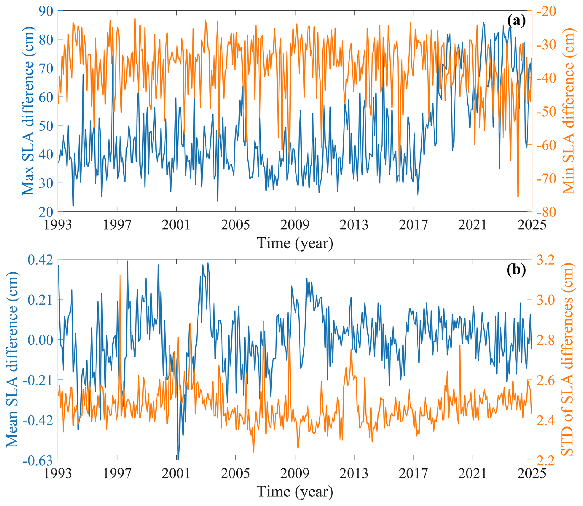
Figure 4 Temporal evolution of monthly global grid-point statistics of SLA differences between the PolyU and C3S products over the period January 1993–December 2024. (a) Monthly maximum and minimum SLA differences. (b) Monthly mean and SD of the SLA differences.

Figure 5 presents the spatial distribution of SLA variance differences between the PolyU and C3S gridded SLA products, computed at each grid point using the monthly SLA time series from January 1993 to December 2024. The variance differences show a clear regional structure, with pronounced signals mainly appearing as negative values in dynamically active regions, while positive values are generally weak and localized. In broad low- to mid-latitude open-ocean regions away from strong currents and coastal zones, variance differences are close to zero and spatially homogeneous, indicating that the two products provide a highly consistent representation of SLA variability in these areas. This consistency suggests that, in regions with weaker mesoscale variability and relatively stable altimeter sampling, the influence of processing methodology on variance levels is limited.

Figure 5 The spatial distribution of the SLA variance differences between the PolyU and C3S products over the January 1993–December 2024 period. Nine representative locations in dynamically active ocean regions, marked by blue dots, are selected for subsequent time-series comparisons.

However, pronounced variance differences are mainly found in dynamically active regions, including western boundary current systems such as the Gulf Stream and Kuroshio, marginal seas, coastal and shelf regions, and the Southern Ocean associated with the Antarctic Circumpolar Current. In many of these regions, the differences are predominantly negative, indicating that C3S generally retains higher SLA variance than PolyU. This pattern is particularly evident in the Gulf Stream Extension, Kuroshio Extension, and the broad quasi-zonal bands of the Southern Ocean. This may reflect differences in along-track preprocessing, crossover adjustment, and the spatial smoothing scales used during gridding. Weak and localized positive differences are present in some regions, but they are less spatially coherent and much less prominent than the negative differences.

Overall, the regions with pronounced negative or positive variance differences mainly correspond to areas characterized by strong wind-driven circulation, intense mesoscale eddy activity, large spatial gradients, and significant temporal variability. In such regions, SLA variance is particularly sensitive to the choice of data processing methods, including along-track preprocessing, crossover adjustment schemes, and the spatial smoothing scales used during gridding. As a result, methodological differences between products can be amplified, leading to noticeable local discrepancies in variance levels. It should be noted that higher SLA variance does not necessarily indicate higher accuracy; rather, the variance differences reflect different methodological trade-offs between signal retention and smoothing stability. Similar regional patterns of variance differences have been reported in intercomparisons of different DUACS product releases (Pujol et al., 2016; Taburet et al., 2019), highlighting that these differences are not unique to PolyU and C3S. Instead, they generally reflect the combined influence of regional ocean dynamics and the specific choices made in data processing and mapping methodologies. Understanding these patterns is crucial for interpreting gridded SLA products, especially in studies focusing on mesoscale variability, coastal processes, and climate change.

4.2 Climate scales

To examine the consistency between the PolyU and C3S gridded SLA products at climate-relevant time scales, sea-level trends, accelerations, and associated uncertainties are compared at both global and regional scales (Figs. 6 and 7). In this study, all sea-level trends are estimated from monthly SLA time series without applying glacial isostatic adjustment (GIA) corrections, in order to ensure a consistent comparison between the two altimetry-based products. Sea-level trends are estimated using ordinary least squares regression, while accelerations are derived from a quadratic fit to the SLA time series. Uncertainties in the estimated trends and accelerations are quantified by accounting for first-order autoregressive AR(1) temporal correlation in the regression residuals (Weatherhead et al., 1998; Mu et al., 2025b) and are reported as 95% confidence intervals. Although AR(1) commonly used to estimate uncertainties, higher-order autoregressive models, such as AR(3) or AR(5), may better represent the temporal correlation structure of the noise. Regardless of the AR order used, the resulting uncertainties represent parameter-estimation uncertainties under the adopted statistical assumptions. These AR-based uncertainties are generally larger than those obtained without considering temporal autocorrelation, because the effective degrees of freedom are reduced. Therefore, the choice of AR model does not affect the estimated trends, accelerations, or the assessment of inter-product consistency in this study. A more rigorous uncertainty assessment would require consideration of multiple error sources, as described in detail by Ablain et al. (2019) and Guérou et al. (2023).

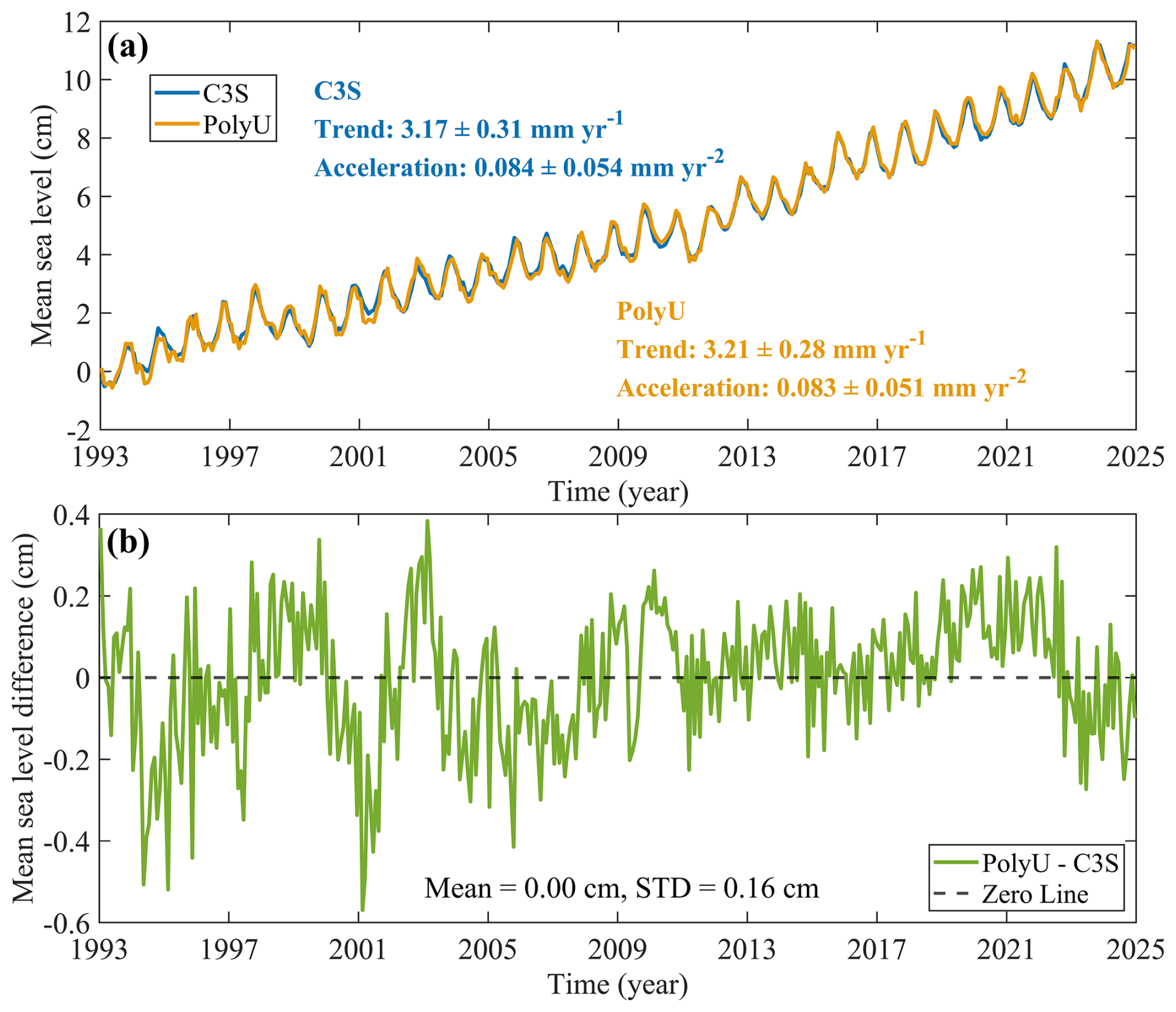
Figure 6 Temporal evolution of the global mean sea-level (GMSL) trend estimated from the PolyU (orange line) and C3S (blue line) gridded SLA products over the period from January 1993 to December 2024. The trend was computed with no GIA correction applied. (a) GMSL time series. (b) GMSL difference (PolyU–C3S).

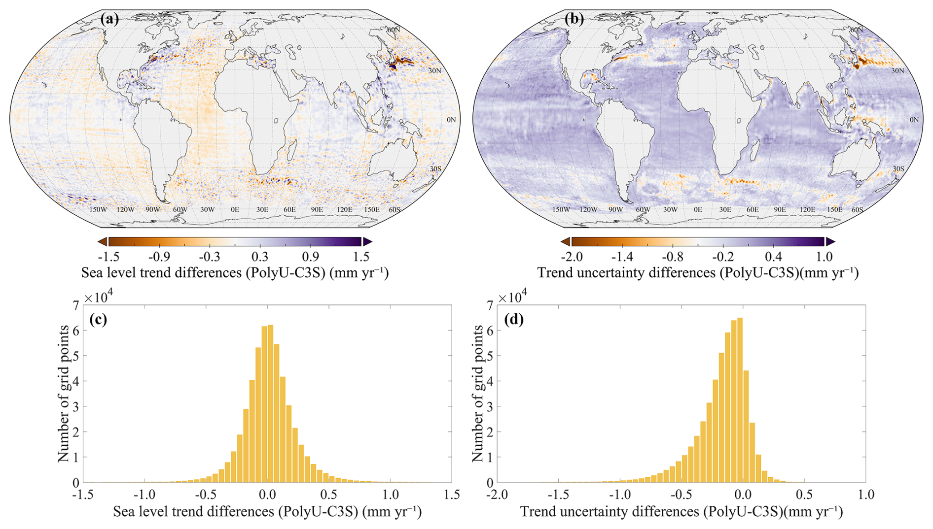
Figure 7 Map and statistical distributions of sea-level trend differences and associated uncertainty between the PolyU and C3S gridded SLA products from 1993 to 2024. (a) and (b) show global maps of sea-level trend differences and their associated uncertainties, respectively. (c) and (d) display histograms of sea-level trend differences and trend-uncertainty differences.

The GMSL time series derived from the PolyU and C3S gridded SLA products show remarkable agreement (Fig. 6). The two records demonstrate a high level of consistency, effectively resolving seasonal variability, interannual variability, and long-term changes with high fidelity. This strong agreement is reflected in the estimated linear trends: 3.21±0.28 mm yr⁻¹ for PolyU and 3.17±0.31 mm yr⁻¹ for C3S. The difference between these trends is only about 0.04 mm yr⁻¹, which is well within the respective uncertainty ranges, indicating that the two products are statistically indistinguishable in terms of global sea-level rise. Similarly, the acceleration estimates for PolyU (0.083±0.051 mm yr⁻¹) and C3S (0.084±0.054 mm yr⁻¹) overlap within their 95 % confidence intervals, indicating there is no significant difference in the inferred acceleration. Further evidence of their consistency is provided by the GMSL difference time series (Fig. 6b), which fluctuates around zero with a mean of 0.00 cm and a SD of 0.16 cm. This demonstrates the absence of any persistent systematic offset between the two products and highlights their reliability for long-term sea-level change analysis. These results highlight the robustness of both PolyU and C3S gridded SLA products for monitoring long-term sea-level changes and support their use in climate research.

Compared to the global-mean results, regional differences between the two products are more pronounced (Fig. 7). Both the sea-level trend estimates and their associated uncertainties exhibit substantial spatial heterogeneity at regional scales, reflecting the influence of local ocean dynamics and data processing choices. Sea-level trend differences (PolyU–C3S; Fig. 7a) are generally close to zero over most ocean basins but show notable positive and negative deviations in specific regions, including western boundary current systems (e.g., the Gulf Stream and Kuroshio), the Southern Ocean, and parts of the mid- to high-latitude oceans. These regions are characterized by strong mesoscale variability and complex dynamical regimes, making regional trend estimates particularly sensitive to differences in along-track preprocessing, crossover adjustment, and spatial mapping strategies. Such sensitivity is well-documented in the literature, as small methodological differences can be amplified in dynamically active areas (Ducet et al., 2000; Pujol et al., 2016; Taburet et al., 2019). The statistical distribution of regional trend differences (Fig. 7c) is approximately symmetric and centered near zero, indicating that there is no systematic global bias in regional trend estimates between PolyU and C3S. This suggests that, despite localized discrepancies, the two products are broadly consistent in their representation of regional sea-level trends.

In contrast, differences in trend uncertainty (Fig. 7b) display a smoother and more spatially coherent pattern. The differences are generally small and close to zero, but they show a slight tendency toward negative values over broad oceanic regions, suggesting that PolyU tends to provide comparable or marginally smaller trend uncertainties than C3S. This is further supported by the histogram of trend-uncertainty differences (Fig. 7d), which peaks near zero but is slightly shifted toward negative values. The lower uncertainties in PolyU may be attributed to its use of LSC for gridding, which explicitly incorporates spatial covariance and observation-error information, potentially contributing to more stable gridded SLA estimates in well-sampled regions. Overall, these results highlight that while both products are consistent at the global scale, regional differences can arise due to the interplay of ocean dynamics and methodological choices.

To further assess whether the regional differences identified in Fig. 7 affect estimates of large-scale sea-level change, basin-scale mean sea-level trends and accelerations for several representative ocean basins are summarized in Table 2. Despite the pronounced spatial heterogeneity in regional trend estimates, the basin-mean trends and accelerations derived from the two products remain highly consistent across the Pacific, Atlantic, Indian, and Arctic oceans. In all basins, the differences in basin-averaged trends between the two products, are substantially smaller than the corresponding 95 % confidence intervals, indicating that any discrepancies are statistically insignificant. Similarly, the acceleration estimates for each basin overlap within their respective uncertainties, further demonstrating the robustness of large-scale sea-level change estimates to methodological differences at the regional level. These findings confirm that, while regional-scale differences can be substantial, particularly in dynamically active or data-sparse regions, they do not propagate into significant discrepancies in basin-scale or global sea-level change estimates between the two products.

Table 2 Basin-scale mean sea-level trends (linear trends) and accelerations derived from the PolyU and C3S gridded SLA products. Linear trends are estimated without applying a GIA correction. Uncertainties are computed by accounting for first-order autoregressive AR(1) temporal correlation in the residuals and are reported as 95 % confidence intervals.

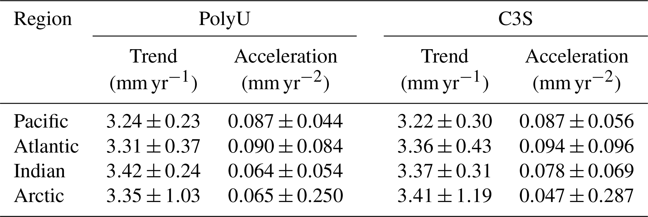
The Arctic basin stands out as an exception, exhibiting comparatively larger uncertainty estimates. This can be attributed to several factors: extensive sea-ice coverage, which limits the availability and quality of satellite altimetry data; reduced data spatial and temporal data coverage; and enhanced low-frequency variability associated with polar processes. These factors collectively reduce the effective degrees of freedom in the time series, especially when accounting for AR(1) temporal autocorrelation, and thus increase the uncertainty in trend and acceleration estimates for the Arctic basin.

As shown in Figs. 5 and 7, the PolyU and C3S gridded SLA products exhibit pronounced differences in certain ocean regions. Specifically, Fig. 5 reflects the differences in SLA variance, while Fig. 7 shows the differences in grid-point trends, and these discrepancies are mainly concentrated in dynamically active ocean regions with large sea-level variability, such as the Antarctic Circumpolar Current (ACC), the East Australian Current (EAC), the Gulf of Mexico (GOM), the Gulf Stream Extension (GSE), and the Kuroshio Extension (KE). Within these regions, nine points were selected (their locations are indicated in Fig. 5), and time series comparisons of the PolyU and C3S SLA products, as well as their differences, were conducted, with the results shown in Fig. 8. Table 3 provides the geographic coordinates of the nine selected points and their corresponding typical ocean regions.

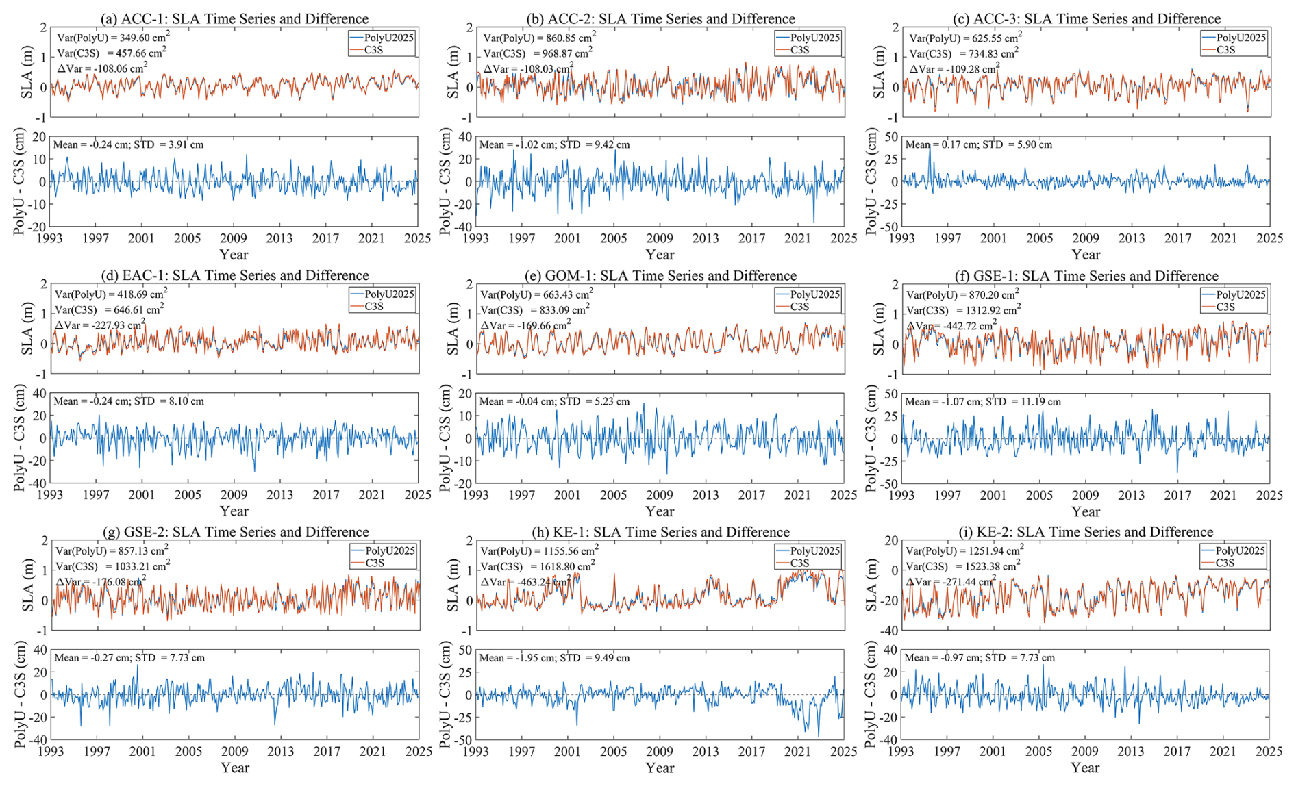
Figure 8 SLA time series and their differences between the PolyU and C3S gridded SLA products at nine selected points (locations shown in Fig. 5).

Table 3 Geographic coordinates of the nine selected points in dynamically active ocean regions.

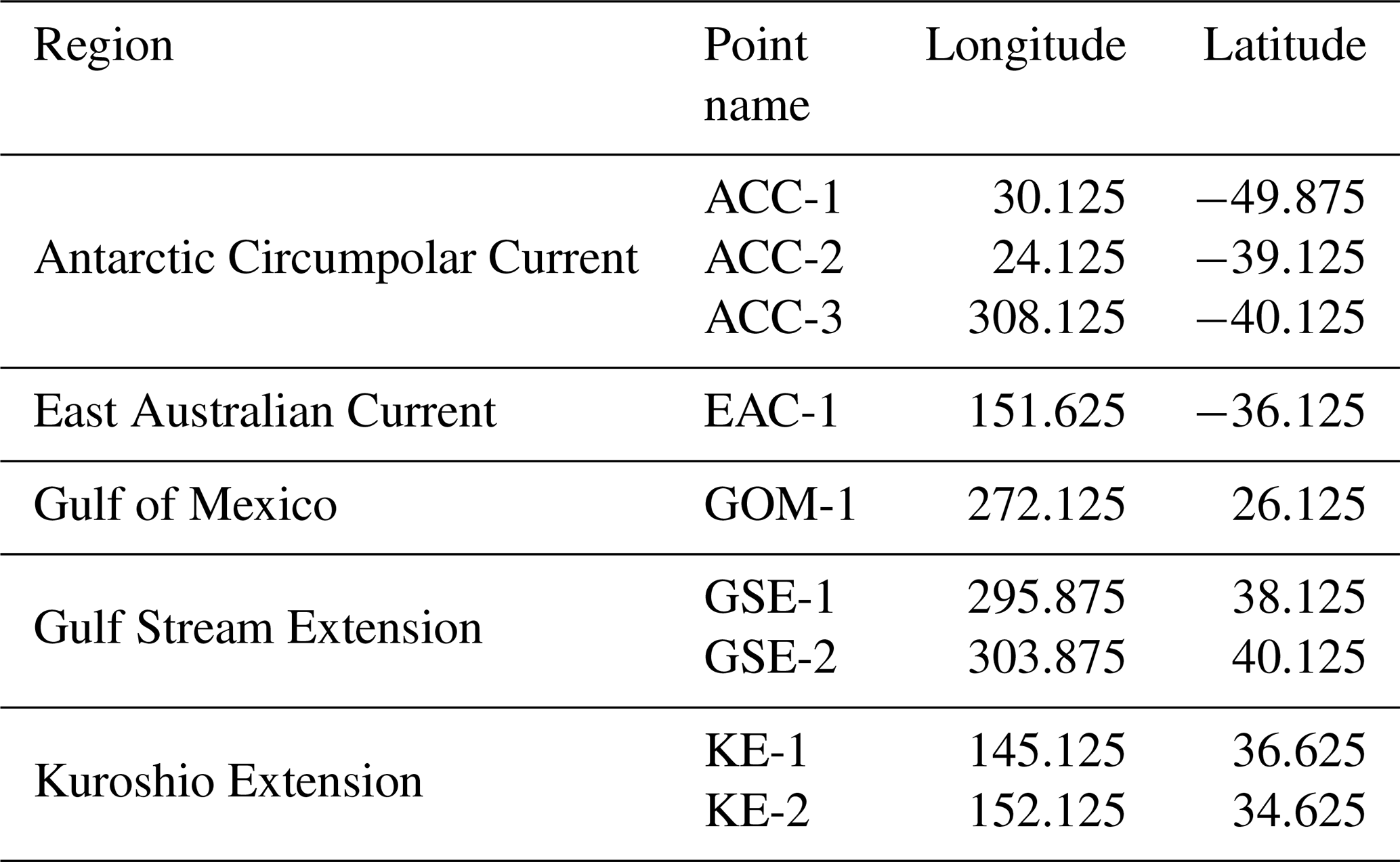
Figure 8 shows that, although these points are located in regions where the PolyU and C3S products exhibit relatively large differences in SLA variance and trends, the overall temporal evolution of the SLA time series from the two products remains generally consistent at each site, capturing the main characteristics of sea-level variability, including seasonal-to-interannual fluctuations. From the difference time series (PolyU–C3S), the mean differences at most points are close to zero, and the variations fluctuate around zero, indicating the absence of a pronounced systematic bias between the two products. However, the SD of the PolyU–C3S difference time series varies considerably among the selected points, indicating that the temporal agreement between the two products is spatially dependent. For example, some points (e.g., GSE-1 and KE-1) exhibit relatively large SDs, suggesting noticeable differences in short-term fluctuations or local variability, whereas others (e.g., ACC-1 and ACC-3) show smaller SDs, indicating better agreement between the two products. In addition, the variance information shown in the figure (Var and ΔVar) also indicates substantial regional differences in variance; however, these differences are primarily reflected in the magnitude of temporal variability and do not substantially change the overall temporal evolution patterns of the two time series.

5 Evaluation against TG observations

A systematic comparison with monthly mean TG observations was conducted to evaluate the consistency of the PolyU and C3S gridded SLA products in coastal and near-coastal regions. Coastal sea-level variability is influenced by a range of complex processes, including tides, wind-driven currents, and local bathymetry, which can make direct comparisons between in situ and satellite-derived measurements challenging. To address this, a time-series-based pairing strategy was adopted, rather than simply selecting the geographically nearest grid point. Specifically, for each TG station, temporal correlations were calculated between the TG time series and surrounding SLA grid points within a 1° search radius around the TG location, following the approach of Sánchez-Román et al. (2023). The grid point yielding the highest correlation with the TG record, computed after removing the linear trend and seasonal signals (annual and semi-annual components) from all three-time series (TG, PolyU, and C3S), was selected to represent the altimetric SLA corresponding to that station. This approach ensures that the comparison is based on the most dynamically consistent grid point, accounting for potential spatial offsets due to coastal geometry, land contamination in satellite footprints, and the influence of local oceanographic features. It should be noted that TG observations are not corrected for vertical land motion.

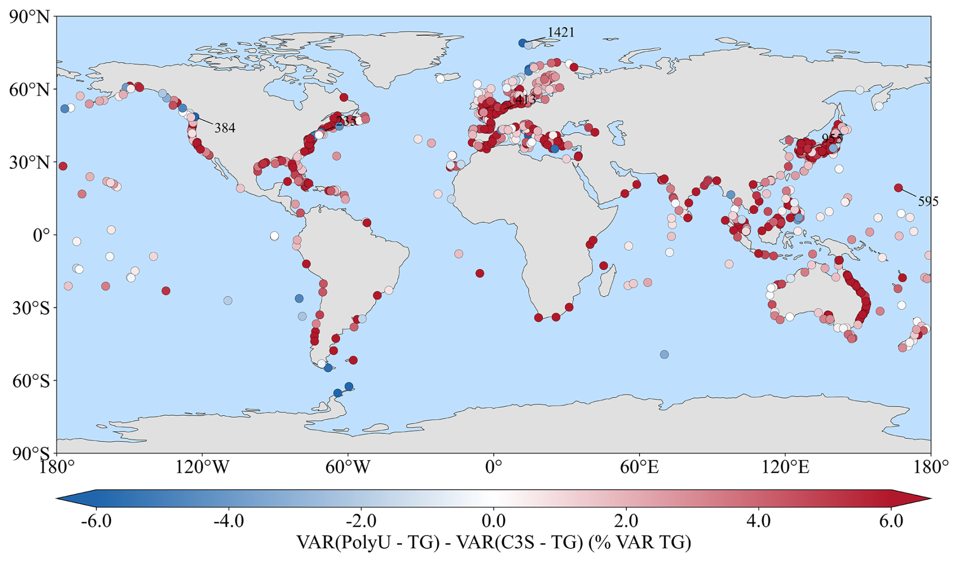
Figure 9 Difference of the variance between gridded products and TG successively using the PolyU and C3S gridded products. The statistic is expressed as a percentage of the variance of the TG observations. Numbers denote TG station identifiers from the PSMSL database, with a subset used for subsequent time-series analysis.

5.1 Coastal differences

For each of the 889 TG stations (see Sect. 2.3), monthly residual time series were computed for the PolyU–TG and C3S–TG pairs based on the corresponding gridded SLA products, and their variances were calculated. The difference between the two residual variances was then normalized by the variance of the TG time series at each station and expressed as a percentage, providing a relative metric for comparing the performance of the two SLA products against TG observations, consistent with the approach of Taburet et al. (2019). The resulting normalized residual variance differences are shown in Fig. 9, where positive values indicate larger residual variance for PolyU–TG, and negative values indicate larger residual variance for C3S–TG.

The spatial pattern of these normalized residual-variance differences reveals notable regional contrasts. Positive values dominate globally and occur mainly in near-coastal and shelf regions, as well as in dynamically active zones. Negative differences are less common and are mostly confined to parts of the open ocean and some high-latitude regions. In low-latitude open-ocean regions, the normalized differences are generally close to zero and spatially homogeneous, indicating similar residual variance for both products.

These features indicate that the residual variances of both the PolyU–TG and C3S–TG time series are sensitive to regional ocean dynamics and to the processing choices applied in the gridded SLA products. In near-coastal and dynamically active regions, sea-level variance is enhanced by mesoscale eddies, boundary currents and other high-frequency processes, and horizontal gradients are sharper. Under these conditions, differences in along-track preprocessing, spatial mapping, and smoothing strategies are more likely to translate into distinct residual variances, as widely discussed in coastal altimetry studies (Vignudelli et al., 2011; Cipollini et al., 2017). In contrast, open-ocean regions are dominated by large-scale and lower-frequency variability, where the different processing strategies tend to converge toward similar fields, so the residual-variance differences remain small. A comparison with Figs. 5 and 7 further supports this interpretation: regions with pronounced residual-variance differences in Fig. 9 largely coincide with areas showing large SLA variance differences (Fig. 5) and stronger discrepancies in linear trends (Fig. 7). This spatial coherence across independent diagnostics indicates a robust and internally consistent regional response of the two gridded SLA products to both dynamical regimes and processing choices.

Based on the spatial distribution of the normalized residual-variance differences shown in Fig. 9, six representative TG stations (IDs: 235, 384, 413, 595, 955, and 1421) were selected for further analysis, and their locations are indicated in the Fig. 9. These stations were chosen from those with relatively complete observational records over the period from January 1993 to December 2024. Among them, stations 235, 384, and 1421 exhibit variance difference percentages of −5.96 %, −15.33 %, and −6.48 %, respectively, corresponding to the largest negative values, whereas stations 413, 595, and 955 show values of 8.81 %, 5.71 %, and 7.56 %, representing the largest positive values. These stations therefore capture the most pronounced positive and negative differences between the two gridded products relative to TG  bservations. Using these stations, a detailed comparison of the SLA time series from PolyU, C3S, and TG was performed (see Fig. 10). The time series shown in Fig. 10 have been detrended and deseasoned.

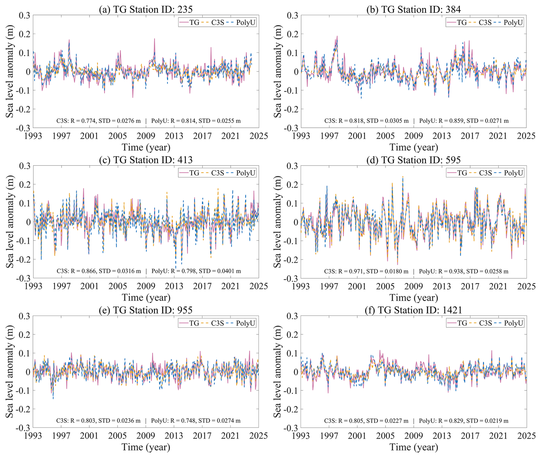
Figure 10 Detrended and deseasoned SLA time series from TG, PolyU, and C3S gridded SLA products at selected stations identified in Fig. 9, illustrating cases with different levels of variance differences. The reported correlation coefficients (R) and standard deviations (SD) are computed from these processed time series.

As illustrated in Fig. 10, both gridded SLA products show a high level of consistency with the TG time series after removing the linear trend and seasonal signals, with correlation coefficients generally exceeding 0.7, indicating good temporal agreement with TG observations. Despite this, these stations correspond to the extreme values of the variance difference percentage shown in Fig. 9, suggesting that, even when the temporal patterns are similar, noticeable differences remain in the variance difference percentage. At stations 235, 384, and 1421, PolyU shows higher correlation coefficients and SD values closer to those of TG, whereas at stations 413, 595, and 955, C3S shows higher correlation coefficients and SD values closer to TG. In addition, the SD values vary among stations, indicating that both PolyU and C3S exhibit deviations from TG as measured by SD, and that these deviations differ between the two products and across locations, even though both products maintain overall good agreement with TG observations.

To further examine how the differences identified in Fig. 9 depend on temporal scale, a scale-decomposition analysis was applied to the detrended SLA–TG residual time series. The decomposition was performed using a multi-scale decomposition based on successive moving averages approach, which is commonly used to separate sea-level variability into different frequency bands (IPCC, 2023; Dangendorf et al., 2014). The residual variability at each tide gauge was decomposed into three components: (i) short-term variability (<1 year), dominated by seasonal to sub-seasonal processes; (ii) interannual variability (1–5 years), associated mainly with climate models such as ENSO and other large-scale ocean–atmosphere oscillations; and (iii) low-frequency variability (>5 years), which includes decadal to multidecadal changes and residual long-term signals not captured by the linear trend. For each temporal band, the variance difference between the PolyU–TG and C3S–TG residuals were computed and normalized by the variance of the corresponding observations, yielding the relative variance difference (ΔVAR). The resulting statistics were then aggregated across all available tide-gauge stations and are summarized in Fig. 11.

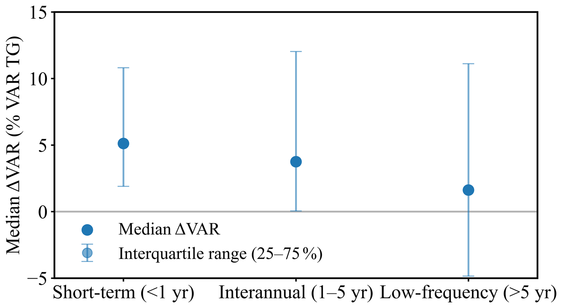
Figure 11 Scale dependence of SLA–TG residual variance differences between PolyU and C3S gridded SLA products. The relative variance difference (ΔVAR) is defined as the difference in variance between PolyU–TG and C3S–TG residuals, normalized by the variance of the TG observations, and expressed as a percentage. Results are presented for three temporal scales: short-term (<1 ear), interannual (1–5 years), and low-frequency (>5 years). Dots represent the median ΔVAR across stations, and error bars indicate the interquartile range (25th–75th percentiles).

The residual variance differences exhibit a clear dependence on temporal scale. At short time scales (<1 year), PolyU–TG residual variance is generally higher than C3S–TG, with a median ΔVAR of approximately 5 %, and ΔVAR values are predominantly positive across TG stations. This suggests that the PolyU product tends to retain higher-frequency variability, which is strongly influenced by local processes and by details of the along-track editing. With increasing time scale, the magnitude and spread of the differences decrease. For interannual time scales (1–5 years), the median ΔVAR is reduced to about 3 %–4 %, and the distribution of ΔVAR becomes noticeably narrower, indicating a closer agreement between the two products in representing climate-driven fluctuations such as ENSO and other basin-scale modes. At longer time scales, corresponding to the low-frequency component (>5 years), the residual variance differences decrease is further diminished: the median ΔVAR is very close to zero and the interquartile range spans zero. Thus, for most stations, PolyU and C3S provide essentially comparable low-frequency residual variability, consistent with the expectation that long-term signals are less sensitive to differences in high-frequency filtering, mapping parameters, or coastal processing. Overall, the residual variance differences are largest at short time scales and progressively weaken toward longer time scales, demonstrating a clear scale dependence in the discrepancies between the PolyU and C3S gridded SLA products.

5.2 Consistency of long-term sea-level trends

Figure 12 presents the spatial distribution and statistical distributions of linear sea-level trend differences between the gridded SLA products and TG observations for the PolyU–TG and C3S–TG comparisons. The spatial patterns (Fig. 12a and b) reveal pronounced heterogeneity, with larger discrepancies predominantly located in coastal regions, western boundary current systems, and parts of the Southern Ocean. These regions are known to be more challenging for satellite altimetry due to land contamination, complex coastal bathymetry, and imperfect geophysical and coastal corrections, which reduce the effective resolution and accuracy of the gridded products. The spatial distribution of these discrepancies is broadly consistent with the regions of enhanced differences identified in Fig. 7, indicating that the TG-based evaluation is consistent with the altimetry-only comparison. This spatial heterogeneity is further reflected in the statistical distributions (Fig. 12c and d), where the trend differences span a relatively wide range but remain generally centered near zero. The mean differences values (0.38 mm yr⁻¹ for Fig. 12c and 0.36 mm yr⁻¹ for Fig. 12d) and the broadly symmetric shapes of the histograms suggest that neither product exhibits a pronounced systematic bias relative to TG observations at the global scale. The spread of the distributions indicates considerable station-level variability, consistent with the localized discrepancies observed in the spatial maps.

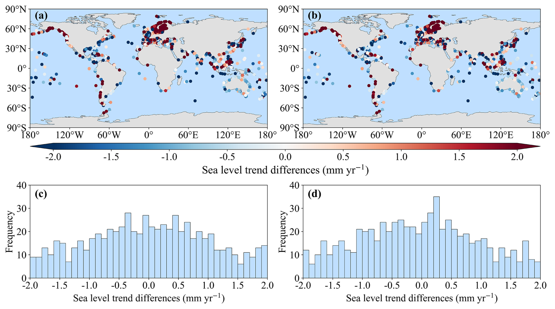
Figure 12 Spatial distribution and statistical distribution of sea-level trend (linear trend) differences between the gridded products and TG observations. For each TG station, trends are estimated from collocated monthly time series over the station-specific valid observation period. Panels (a) and (b) show the spatial distribution of trend differences for PolyU–TG and C3S–TG, respectively, while panels (c) and (d) present the corresponding histograms, summarizing the frequency distribution of these differences across all stations.

A comparison of Fig. 12a–d shows that the PolyU–TG and C3S–TG results exhibit very similar spatial patterns and comparable statistical distributions, suggesting a consistent large-scale representation of long-term sea-level trends. The differences between the two products are primarily manifested in the magnitude and dispersion of the trend differences, rather than in coherent regional structures, indicating that they are dominated by localized variations at individual stations. These differences likely reflect distinct choices in coastal processing, mapping strategies, and the treatment of along-track measurements.

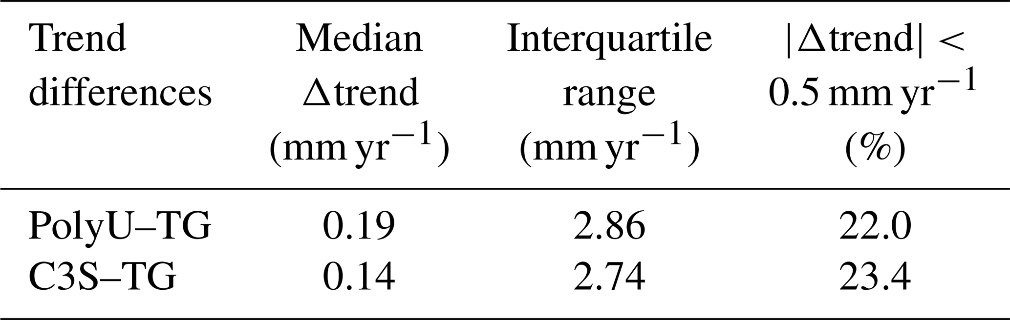
To quantify the overall characteristics of the trend differences, Table 4 summarizes several key statistical metrics across all TG stations. These include the median Δtrend (defined as the difference between the trend from the PolyU or C3S gridded SLA products and the corresponding TG trend), the interquartile range (IQR; 75th–25th percentiles), and the percentage of stations with $\left|\mathrm{\Delta }\mathrm{trend}\right|<\mathrm{0.5}$ mm yr?⁻¹. The median Δtrends are 0.19 mm yr⁻¹ for PolyU–TG and 0.14 mm yr⁻¹ for C3S–TG, both close to zero, indicating that, on average, the long-term trend from the two gridded SLA products agree well with TG estimates and show only small systematic biases. The IQR are 2.86 mm yr⁻¹ for PolyU–TG and 2.74 mm yr⁻¹ for C3S–TG, which are nearly identical, implying a similar spread in station-scale discrepancies. In addition, the percentages of stations with $\left|\mathrm{\Delta }\mathrm{trend}\right|<\mathrm{0.5}$ mm yr⁻¹ are 22.0 % for PolyU–TG and 23.4 % for C3S–TG, further demonstrating broadly comparable skill relative to TG observations. The small numerical differences between PolyU and C3S are well within the range expected from natural variability, measurement noise, and methodological differences in gridding and corrections. Overall, Table 4 indicates a high degree of consistency between PolyU and C3S in estimating long-term sea-level trends, with residual differences dominantly reflecting localized, station-specific effects rather than systematic global discrepancies.

Table 4 Summary statistics of sea-level trend differences between the gridded products (PolyU and C3S) and TG observations.

5.3 Performance in open-ocean conditions

To further investigate the spatial trend differences observed in Fig. 12 while minimizing the influence of coastal complexity, a subset of 27 open-ocean TG stations was selected from the full set of 889 stations (see Sect. 2.3). These 27 stations are located on small islands in broadly open-ocean settings and are therefore less affected by coastal dynamics (as shown in Fig. 13c). All selected stations have data completeness exceeding 90 % over the period from January 1993 to December 2024. For stations with incomplete records, the PolyU and C3S SLA time series are temporally aligned with the corresponding TG observations, and only overlapping months are used in the subsequent scatter, trend, and acceleration analyses. This subset provides a complementary benchmark for evaluating the performance of gridded SLA products under relatively well-resolved open-ocean conditions.

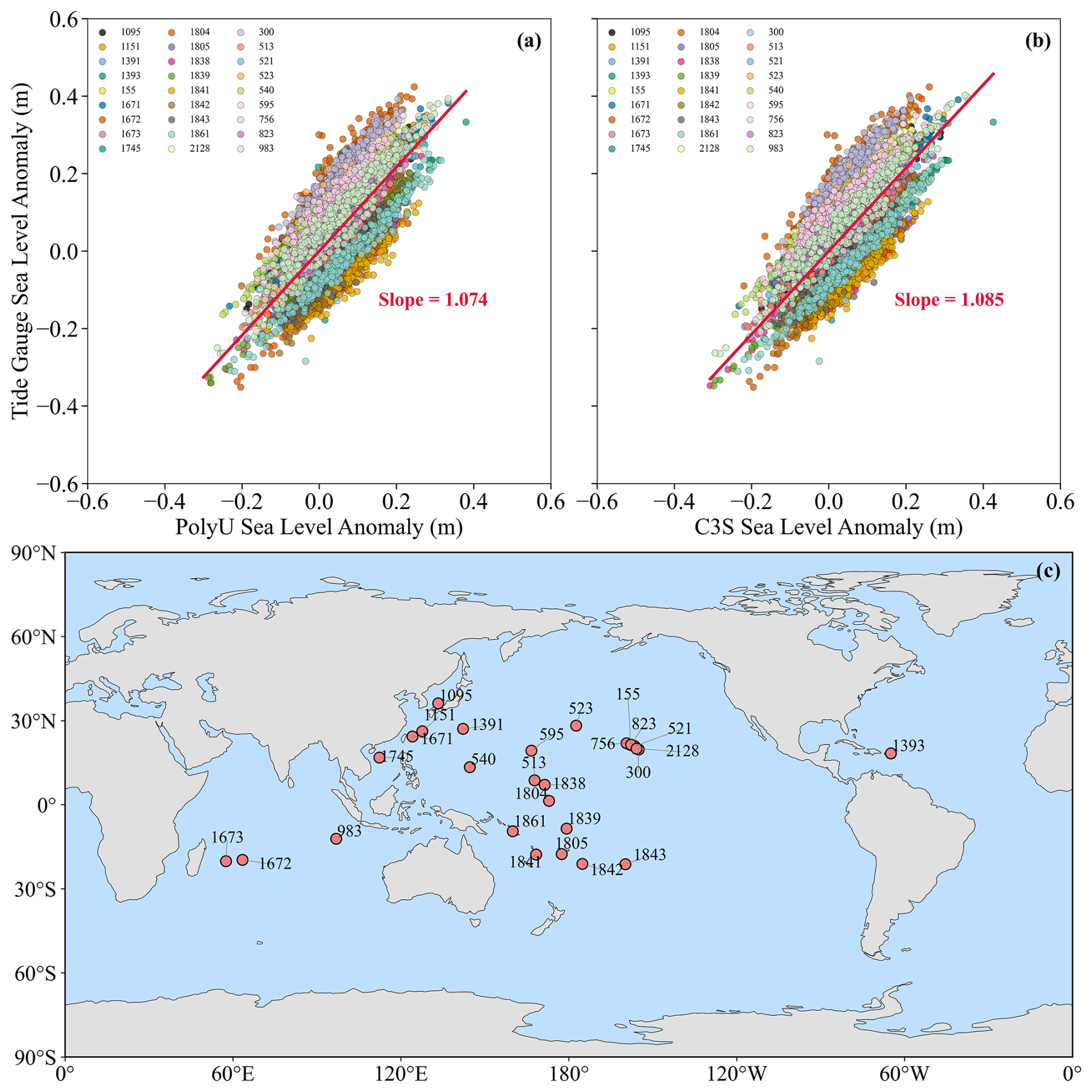
Figure 13 Comparison of SLA from the PolyU and C3S gridded SLA products with TG observations at 27 open-ocean TG stations. (a) Scatter plot of SLA from the PolyU gridded SLA product versus TG observations. (b) Scatter plot of SLA from the C3S gridded SLA product versus TG observations. (c) Geographical distribution of the 27 selected TG stations, with station identifiers from the PSMSL database.

Figure 13 compares the agreement between the PolyU and C3S gridded SLA products and TG observations at these 27 stations. Figure 13a and b shows scatter plots of PolyU–TG and C3S–TG SLA, respectively, and Fig. 13c presents the geographical distribution of these 27 stations. Both products exhibit a clear linear correspondence with TG observations, as indicated by the close alignment of the scatter points with the 1:1 reference line in both the PolyU–TG and C3S–TG comparisons. However, systematic differences remain in their response ratios and scatter characteristics. For PolyU–TG (Fig. 13a), the regression slope is 1.074 and the point cloud is relatively compact, indicating a response ratio to TG SLA slightly greater than unity with limited dispersion. In contrast, the C3S–TG comparison (Fig. 13b) shows a marginally higher regression slope (1.085) together with a more dispersed distribution, particularly at larger SLA values, suggesting a slightly stronger response to TG SLA variability accompanied by increased local scatter.

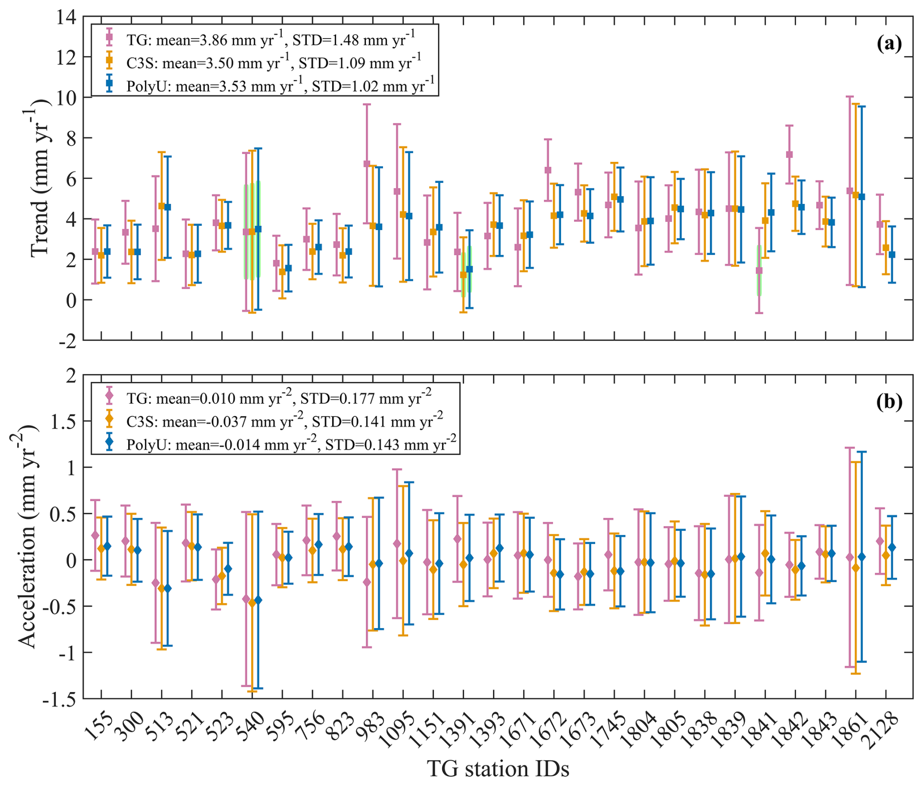
Figure 14 Comparison of linear sea-level trends and accelerations estimated from monthly SLA time series at 27 selected open-ocean TG stations, using TG observations and the PolyU and C3S gridded SLA products. (a) Linear trends and (b) accelerations estimated for the station-specific valid observation periods. The mean values and standard deviations  SD) represent spatial statistics across the 27 selected open-ocean tide-gauge stations, derived from TG observations and the corresponding PolyU and C3S gridded SLA products, respectively. Error bars represent 95 % confidence intervals, accounting for AR(1) temporal correlation. Green markers indicate stations where the uncertainty exceeds the trend magnitude. Station identifiers are from the PSMSL database.

Figure 14 compares linear sea-level trends and accelerations estimated from monthly SLA time series at the 27 selected open-ocean TG stations, using TG observations and the PolyU and C3S gridded SLA products. Both products yield linear sea-level trends (Fig. 14a) and accelerations (Fig. 14b) that are broadly consistent in magnitude and sign and that generally fall within the range indicated by TG observations. This consistency is also reflected in the spatially averaged estimates across the 27 stations. The mean trends are 3.53 mm yr⁻¹ for PolyU and 3.50 mm yr⁻¹ for C3S, compared to 3.86 mm yr⁻¹ from TG observations. Similarly, the mean accelerations are −0.014 mm yr⁻¹ (PolyU) and −0.037 mm yr⁻¹ (C3S), which are comparable to the TG estimate of 0.010 mm yr⁻¹. These results indicate that both products capture the large-scale characteristics of long-term sea-level change in open-ocean regions, with no substantial systematic offset relative to TG observations. However, distinct differences emerge at station scale. For the trends (Fig. 14a), C3S shows a noticeably larger spread among stations and systematically wider confidence intervals. At several stations, the C3S trend deviates more from the TG central estimate. PolyU trends, in contrast, are more tightly clustered, exhibit narrower uncertainty ranges, and tend to lie closer to the TG values, indicating a more constrained representation of long-term change.

The contrast is even clearer for accelerations (Fig. 14b). C3S yields relatively larger positive or negative accelerations at several stations, accompanied by increased uncertainties; in some cases, the confidence intervals approach or exceed the estimated acceleration, suggesting that part of the signal may reflect unresolved interannual–decadal variability rather than robust acceleration. PolyU accelerations are more uniformly distributed around zero, with smaller inter-station scatter and reduced error bars, pointing to greater temporal stability. When compared with TG estimates, PolyU generally shows better agreement both in the magnitude of acceleration and in the associated uncertainty. Overall, Fig. 14 indicates that while PolyU and C3S a coherent overall picture of long-term sea-level rise and its possible acceleration in the open ocean, PolyU yields smoother and more stable trend and acceleration estimates, whereas C3S preserves stronger local variability, leading to larger dispersion and uncertainty at the individual-station level.

6 Data availability

The PolyU2025 SLA product is openly available at https://doi.org/10.5281/zenodo.17810525 (Yuan et al., 2025) as annual NetCDF (.nc) files, following the standardized naming convention “dt_global_L4_yYYYY_m01–m12.nc” (e.g., dt_global_L4_y1993_m01–m12.nc). Each annual file contains three core variables: monthly SLA fields for January to December (months 1–12) of the corresponding year, longitude, and latitude, all defined on a consistent global grid to facilitate seamless analysis across the full 32-year record from January 1993 to December 2024.

To facilitate temporal visualization, an animation file (dt_global_L4_y1993–2024_m01–12.gif) is provided, illustrating monthly global SLA variability throughout the 32-year record. The animation reveals spatially coherent features and temporal fluctuations linked to major climate variability and long-term oceanographic processes.

7 Discussion and conclusion

This study applied a fully independent processing framework to generate a global 0.25°×0.25° monthly gridded SLA dataset, referred to as PolyU2025 SLA. The dataset presently covers the period from January 1993 to December 2024 and is designed to be updated on a routine basis. A systematic evaluation of PolyU2025 was conducted against the widely used C3S gridded SLA product and against independent TG observations. The comparison is used to assess how PolyU gridded SLA product represents sea-level variability across different spatial and temporal scales and examine the methodological and dynamical processes that underpin similarities and differences among the products.

At the global scale, PolyU and C3S show a very high level of consistency. Global-mean monthly SLA differences fluctuate around zero without any discernible drift, and the corresponding GMSL time series exhibit statistically indistinguishable trends and accelerations, with overlapping uncertainty ranges. Thus, despite the use of different along-track processing schemes and mapping methods, both products recover a coherent global sea-level rise signal over the satellite altimetry era. This agreement confirms that PolyU2025 meets the requirements for climate applications that focus on global or basin-scale sea-level change, such as those considered in IPCC assessments.

In contrast, differences between products become more evident at regional scales and in dynamically energetic regions. Spatial patterns of SLA variance differences, regional trend differences, and residuals relative to TG observations consistently show that discrepancies are concentrated in western boundary current systems, marginal seas, continental shelf regions, and the Southern Ocean. These regions are characterized by intense mesoscale eddy activities, strong spatial gradients, and complex wind-driven and thermohaline processes. They also correspond to areas where sea-level variability is strongest and where satellite altimetry products are most difficult to construct (Vignudelli et al., 2011; Cipollini et al., 2017).

Within such regions, differences between PolyU and C3S in SLA variance levels, trend magnitudes, and uncertainty estimates are significantly amplified. This behavior indicates that regional sea-level variability is highly sensitive to processing choices. These include along-track preprocessing, crossover adjustment schemes, and the specification of correlation scales and error models in spatial mapping. Similar features have been reported repeatedly in intercomparisons of DUACS reprocessed products. They are generally attributed to the combined influence of regional ocean dynamics and methodological differences (Pujol et al., 2016; Taburet et al., 2019).

From a methodological perspective, these regional differences do not appear as systematic positive or negative biases. Instead, they mainly reflect different trade-offs in the representation of variance levels, local trend amplitudes, and uncertainty estimates. PolyU applies a two-step crossover adjustment strategy combined with LSC gridding. This approach constrains spatial and temporal error correlations and leads to a gridded field that is smoother and more stable at long time scales. By contrast, the OI mapping framework used in C3S retains stronger local and mesoscale variability (Ducet et al., 2000; Pujol, et al., 2016).

This methodological contrast is particularly evident in the spatial distribution of monthly SLA variance. PolyU exhibits relatively enhanced or reduced variance in some coastal and boundary-current regions. C3S, on the other hand, preserves higher variability in high-latitude open-ocean regions, especially in the Southern Ocean. Similar regional contrasts have also been identified between successive DUACS reprocessing versions. These results highlight the inherent trade-off between signal retention and smoothing stability in gridded SLA construction.

The comparison with TG observations further supports this interpretation. The spatial distribution of residual variances in the PolyU–TG and C3S–TG comparisons closely mirrors the variance differences observed between the two gridded SLA products. Residuals are substantially larger in coastal, shelf, and dynamically active regions. In contrast, they are generally smaller and more spatially homogeneous in low-latitude open-ocean regions. This indicates that in regions dominated by enhanced small-scale and mesoscale variability, the sensitivity of gridded altimetry products to processing choices is more clearly expressed in their residuals relative to TG observations. This issue has been widely discussed in coastal altimetry studies (Vignudelli et al., 2011; Cipollini et al., 2017).

A particularly noteworthy result is the strong time-scale dependence of the differences between products. At short time scales (<1 year), residual-variance differences between PolyU and C3S relative to TG observations are most pronounced. These differences progressively decrease as the time scale increases. At low-frequency scales (>5 years), they become negligible. This behavior indicates that the primary differences between PolyU and C3S are associated with the representation of short-term and mesoscale variability. In contrast, their representations converge at longer, climate-relevant time scales. This scale dependence is consistent with the patterns observed in SLA variance and regional trend differences, and together these results indicate that the main differences between the two products arise from short-term and mesoscale variability rather than from long-term signals. This provides further support for the consistency of PolyU and C3S in long-term sea-level change analyses.

Further improvements in coastal and short-timescale SLA reconstruction may be achieved by enhancing the quality of near-coastal along-track observations and refining the mapping strategy. In future reprocessing, coastal-oriented waveform retracking and stricter quality control could be applied to reduce land contamination and retain more reliable observations near the coast. Regionally optimized geophysical corrections, especially for tides, wet tropospheric effects, DAC, and sea state bias, may further reduce residual coastal errors. In addition, adaptive covariance scales or error models in the gridding procedure could be considered to better represent the stronger spatial gradients and short-timescale variability in coastal regions. The inclusion of observations from the Surface Water and Ocean Topography (SWOT) mission, TG records, or regional ocean model information may also help improve the reconstruction of coastal SLA variability.

Regarding long-term trends and accelerations, PolyU and C3S show overall consistency when compared with TG observations. Median Δ trend relative to TG are close to zero. The dispersion of differences is comparable between the two products, and most stations fall within the range of natural variability. In the analysis based on 27 open-ocean TG stations, both products successfully reproduce sea-level variability at monthly and climate-relevant time scales. However, at the station scale, PolyU trend and acceleration estimates exhibit a more compact distribution and smaller uncertainties. In contrast, C3S results show greater dispersion. This suggests that PolyU provides enhanced temporal stability in long-term sea-level estimates, whereas C3S remains more sensitive to local variability. As a result, C3S tends to exhibit larger uncertainties in trend and acceleration estimates.

In summary, the PolyU and C3S gridded SLA products are highly consistent in their representation of sea-level change at global and basin scales and are both suitable for long-term sea-level change studies. Differences between the two datasets mainly emerge at regional and short time scales, particularly in dynamically active regions with strong sea-level variability. These differences do not reflect systematic biases but rather result from different methodological choices and trade-offs between signal preservation and smoothing stability. By adopting an independent and comprehensive processing framework, PolyU provides a complementary realization within the family of gridded SLA products, contributing to a more robust multi-product perspective on regional sea-level variability, uncertainty, and product selection for different scientific objectives.