Link-based European road transport emissions for CAMS-REG v8.1 and a comparison to city inventories

Spatially resolved estimates of road transport emissions are fundamental for tackling challenges of air pollution and greenhouse gas emissions. Emission estimates at 0.05° × 0.1° resolution are provided in the widely used CAMS-REG regional European emissions inventory. Building on previous work by Kuenen et al. (2022) for the road transport sector, several improvement opportunities were identified: Firstly (1) an underestimation of ca. 35 % of NO_x emissions in comparison to 8 independent urban inventories; secondly (2), artefacts in the spatial distribution in Eastern European non-EU countries; thirdly (3), the necessity of labour-intense downscaling methodologies to create high-resolution urban inventories from the fixed resolution dataset. To overcome these, emissions for most road links in the domain (n = 59 710 490) were estimated using gap-filled activity data (AADT) from OpenTransportMap, targetting NO_x for the base year 2018. Gap filling was performed with random forest models trained on land-use and road information data and with a spatial method for small roads. For non-EU countries, model performance was R²: 0.63, MAE(AADT): 2028, for EU countries it was R²: 0.74, MAE(AADT): 1570, with better performance for larger roads. Up-to-date emission factors for NO_x were applied on road links using a novel maximum-speed–based classification. To generate the CAMS-REG v8.1 inventory, the resulting spatial distribution was used as a proxy map, together with national totals.

The new dataset is based on OpenStreetMap geometries and lowered the difference to city inventories to 18 % for absolute NO_x emissions. It can be flexibly gridded to high resolutions. Some non-EU cities see large increases (Kiev, +84 %, Istanbul, +360 %) in attributed emissions due to the updated spatial distribution. Two case studies (London and Milan) show an increased spatial correlation, from R²≈0.3 using CAMS-REG v4.2 to R²≈0.6, with CAMS-REG v8.1 against the local inventory. Vector and gridded versions of the emission dataset and spatial distribution are available at https://doi.org/10.5281/zenodo.15688722 (Hohenberger et al., 2025).

1 Introduction

Emission inventories are a fundamental starting point for modelling and policy analysis for both greenhouse gases (GNG) and air pollutants. Coupled with air quality models, they are used to derive pollutant concentrations (El-Harbawi, 2013), epidemiological studies (World Health Organization, 2021), exposure analysis (Isakov et al., 2009), source apportionment (Hopke et al., 2022) or sectoral analysis (Gu et al., 2018). Road transport is a major source of air pollution and GHG emissions. Shares of Europe-wide emissions were as high as 20.6 % for CO, 35.1 % for NO_x, 15.3 % for PM₁₀ and 13.7 % for PM_2.5 in 2022 (EMEP Centre of Inventories and Predictions, 2023). Road transport plays an important role in exposure to air pollutants, especially in cities (Nieuwenhuijsen, 2016; Gurram et al., 2019), where children and households in poverty are often overly affected from exposure to road-based air pollution (Barnes et al., 2019). Contributions to PM_2.5 emissions in urban areas throughout 150 European cities are on average 15 % (Thunis et al., 2023). Increasing the spatial resolution of emission inventories beyond the typical kilometre-scale is important especially for urban applications. The use of low-resolution emission data in urban areas has been found to underestimate health effects (Gurram et al., 2019). In cities, larger population density meets relatively high emissions, for example from road transport, and often complex urban terrains, which can result in steep concentration gradients (Santiago et al., 2021; Fu et al., 2020). Together, these features require higher resolution emission inventories as a basis for different modelling techniques (Kadaverugu et al., 2019; Yang et al., 2019).

In Europe, city-scale emission inventories are available for a number of major cities, including London, Paris, Barcelona and Helsinki (see Sect. 2.1.4). Here, the cost, effort and knowledge needed for inventory preparation can be a barrier for administrations, which limits urban modelling and planning efforts at this level.

In an attempt to increase the spatial resolution, it is possible to downscale existing gridded national, regional or global inventories. This downscaling is performed using proxies such as local road geometries, road type or activity data (Trombetti et al., 2017; Valencia et al., 2022). Manual downscaling using proxy data is again labour intensive, and requires careful data handling and result verification. This can be mitigated by tools such as UrbEm, which is available for European cities to downscale regional emissions to city scale (Ramacher et al., 2021).

Combined with emission factors and fleet composition information, a complete set of roadside activity data allows the calculation of road-level emissions, thus circumventing the need for re-gridding or downscaling of a fixed-size inventory. Roadside activity data is often given in the form of AADT (Annual Average Daily Traffic). However, available activity data for roads is often incomplete. Wherever necessary, gap filling activity data is therefore an important exercise for calculating complete roadside emission. Methods for predicting missing AADT values include statistical modelling and machine learning methods. Recent studies could show improved results with neural networks and tree-based methods compared to statistical approaches (Han, 2024; Sekuła et al., 2018). Amongst the machine learning approaches used to estimate AADT data, random forest (RF) is a common choice among transport modellers (Wen et al., 2022; Baffoe-Twum et al., 2023; Das and Tsapakis, 2020; Sekuła et al., 2018; Antonczak et al., 2025). Random forest models are flexible when working with missing and incomplete data (Tang and Ishwaran, 2017).

The European Copernicus Atmosphere Service (CAMS) maintains a number of regional and global air quality and GHG emission inventories for anthropogenic and biogenic emissions (Denier van der Gon et al., 2023). Amongst them, CAMS-REG-ANT (hereafter CAMS-REG) is an emission dataset covering UNECE-Europe at 0.05° × 0.1° resolution, and is used in the CAMS Regional Air Quality Production System (Colette et al., 2025), as well as in a wide number of studies on air quality and public health (recent studies include: Khomenko et al., 2023; Achebak et al., 2024; Chang et al., 2024). In CAMS-REG, reported country emission sector totals are distributed spatially via gridded proxy maps on a national level, without any prior intermediate regionalisation steps (e.g. to provinces or municipalities). A detailed overview on CAMS-REG is available at (Kuenen et al., 2022). The spatial distribution of road emissions in CAMS-REG has not been updated since version 4.

This study aims to update on the approach and dataset described by Kuenen et al. (2022), focussing on NO_x. There is a growing pool of studies aiming at verifying modelled transport emissions with measured air pollution concentration in European cities. The degree of underestimation is highly variable throughout cities and methodologies. In the following, an overview on recent studies and a subsequent summary of the most important findings is given.

Reported underestimation of modelled concentration is common throughout cities in Europe. Skoulidou et al. (2021) report the degree of underestimation at traffic sites for NO_x in Athens at −10 % (mean bias) against measurement stations; and at −2 % to −35 % against spectroscopy based MAX-DOAS measurements. In Hamburg, the degree of underestimation for NO₂ at four traffic sites was given at 20 % (Karl et al., 2024). Pültz et al. (2025) further find a systematic underestimation throughout urban background NO₂ sites in Germany. Kuik et al. (2018) finds an underestimation of urban NO₂ of 30 % at the urban background and of 50 % at the urban core in the Berlin metropolitan area. A study focussing on Barcelona finds a much lower attribution of PM_2.5 and BC emissions to the transport sector in CAMS-REG, compared to the HERMES emission model (10 % in CAMS-REG compared to 70 % in HERMES) (Navarro-Barboza et al., 2024). Underestimation of transport emissions are further mentioned for Marseilles (Karl et al., 2023) and Liège (Ramacher et al., 2025). Throughout these recent studies, the underestimation of urban transport emissions for NO_x in European cities was thus found to range between 10 %–50 %.

Out of the presented works, Skoulidou et al. (2021), Navarro-Barboza et al. (2024), and Karl et al. (2024) directly use the CAMS-REG inventory, and are thus highly relevant for this study. The spatial distribution is given as a common reason for the found underestimation (see Karl et al., 2023; Pültz et al., 2025; Kuik et al., 2018). Apart from the spatial distribution, further other reasons are presented. In their model setup, Kuik et al. (2018) discuss boundary layer height and model mixing as potentially impacting their results. Moreover, Kuik et al. (2018) discuss the uncertainty of activity data and emission factors, and Pültz et al. (2025) highlight the potential impact of a misallocation of cold starts away from the urban core.

Lastly, the spatial distribution in previous CAMS-REG versions in non-EU Eastern European countries such as Ukraine or Russia showed a number of artifacts (see Fig. 5), where a large portion of the country's emission is attributed to a single pixel or road. For Ukraine, the highway E105 between Dnipro and Kharkiv received the largest share of national emissions, with emission values far exceeding the largest cities in the country. For Russia, a similar distribution was noticed between the highway M-11 between Moscow and St. Petersburg. Moreover, city emissions for non-EU large cities were not on levels comparable with other European cities (see Sect. 3.4). These artifacts are linked to the low level of road information available at the time of preparation and the activity data estimation method described in Kuenen et al. (2022).

Our update to the road transport emission distribution therefore targetted:

1. an inventory on the level of OSM road segments (road vectors, in the following also called road links) that can be flexibly scaled to high resolution and urban scenarios;

2. a distribution of more emissions to urban areas, in line with previous comparisons based on city inventories and previous studies; and

3. a reduction of artefacts, especially in non-EU Eastern Europe.

The new distribution has been included in CAMS-REG since v8, with v8.1 being the latest published version. While staying close to the datasets used in previous CAMS-REG versions for consistency, we attempted to update the spatial distribution based on gap filling of activity data and urban/rural status for all road classes. We further updated the emission factor set, and produced vector-based emissions for the majority of roads within our domain. These were then gridded to city scale, and compared with the best available urban inventories, which is further explained in the methodology (Sect. 2). Section 3 presents the results of our model, and shows comparisons with a number of urban inventories and the spatial distributions of previous CAMS-REG versions. The discussion can be found in Sect. 5, and data availability is described in Sect. 4.

2 Methodology

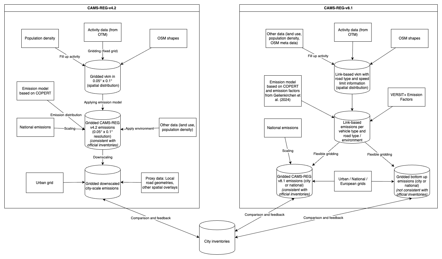
Figure 1 gives an overview on the methodology changes between CAMS-REG 4.2 and CAMS-REG 8.1. The following subsections describe the components of the methodology, data, emission factors, statistical methods and evaluation criteria in detail. Section 2.4 compares the methodology to the previous methodology of the spatial road transport distribution used in CAMS-REG versions 4.2-8.1. All updates presented in this work are included in CAMS-REG since v8.0.

Figure 1 Overview of CAMS-REG-4.2 and CAMS-REG-8.1 methodologies for road transport.

2.1 Data used

2.1.1 Transport data

The road vector dataset used in this study was retrieved from OpenStreetMap (OpenStreetMap contributors, 2023). Information on sidewalks, number of lanes, one-way street status, road type and speed limit was extracted from the OSM dataset with the help of parsing functions wherever available. Speed limits in mph were transformed to km h⁻¹ to achieve a consistent dataset using a function that scans the speed limit entry for “mph” and applies the conversion factor.

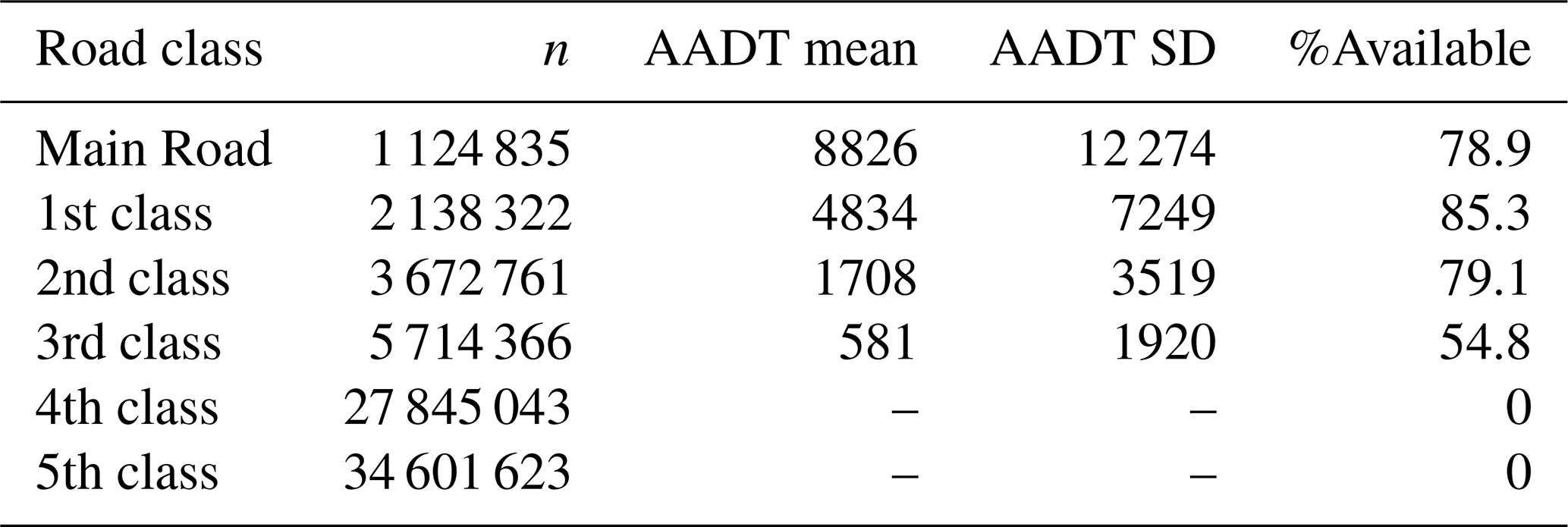
We used the OpenTransportMap dataset (Jedlicka et al., 2016) for link-level activity in the form of AADT. OTM divides roads into six categories ranging between main roads and fifth-class roads. A detailed methodology is available in Jedlicka et al. (2016). Additionally, information on the surface of the road, speed limit and the road capacity is available. The dataset offers substantial information on road activity, especially for major roads. However, there are large data gaps especially for smaller roads, and no AADT values are provided for the smallest road classes, while the majority of individual links in the fourth or fifth class (Table 1). The OTM dataset was then combined with OSM geometries and data columns using a shared reference column. OTM data is available for all 27 EU countries, as well as the UK, Norway and Switzerland. For non-EU countries in the Eastern European region but included in the CAMS-REG domain (e.g. Ukraine, Serbia, western Russia), traffic data from OTM was not available.

Table 1 Data availability and general statistics on OTM data. %Available shows the share of non-zero AADT values for all roads. AADT SD shows the Standard Deviation of AADT values within a road class.

2.1.2 Countries in the study area

The study area covers UNECE-Europe, including the whole of Turkey and the European part of Russia (up to 60° E). Countries in the study area, but without available OTM data are Albania, Bosnia, Serbia, Moldova, Belarus, Ukraine, Russia, Georgia, Azerbaijan, Armenia and Cyprus. For these countries, spatial distributions were derived fully using gap filling models (see Sect. 2.3).

2.1.3 Spatial data

We obtained the CORINE land cover dataset (2018 version) from Copernicus Land Monitoring. This dataset gives high-resolution information on land use in a 100 × 100 m raster grid, and 44 categories for 39 European countries, but excluding large countries within our domain such as Russia, Ukraine and Belarus (Copernicus, 2018). The land-use classes are roughly divided into artificial surfaces, agriculture and forest/natural areas. The data was kept in its initial resolution.

To obtain land use information for the part of the study domain where CORINE was not available, we further used the ESA Worldcover dataset (Zanaga et al., 2022). ESA Worldcover consists of 11 land use classes with global coverage at a 10 m resolution.

For population density data, we queried the LandScan Global dataset for the year 2021 (Bhaduri et al., 2002). The dataset is in a resolution of 30 arcsec (approximately 1 km), and gives values for urban and rural population within each grid cell. Landscan data was available for the entire study domain.

We then extracted spatial information from the aforementioned mentioned raster datasets for each OSM link, which was then used for training and predicting of gap filling models to generate missing traffic density values (see Table 3). Additionally, country information was added with the help of a country mask.

2.1.4 City road traffic emission inventories

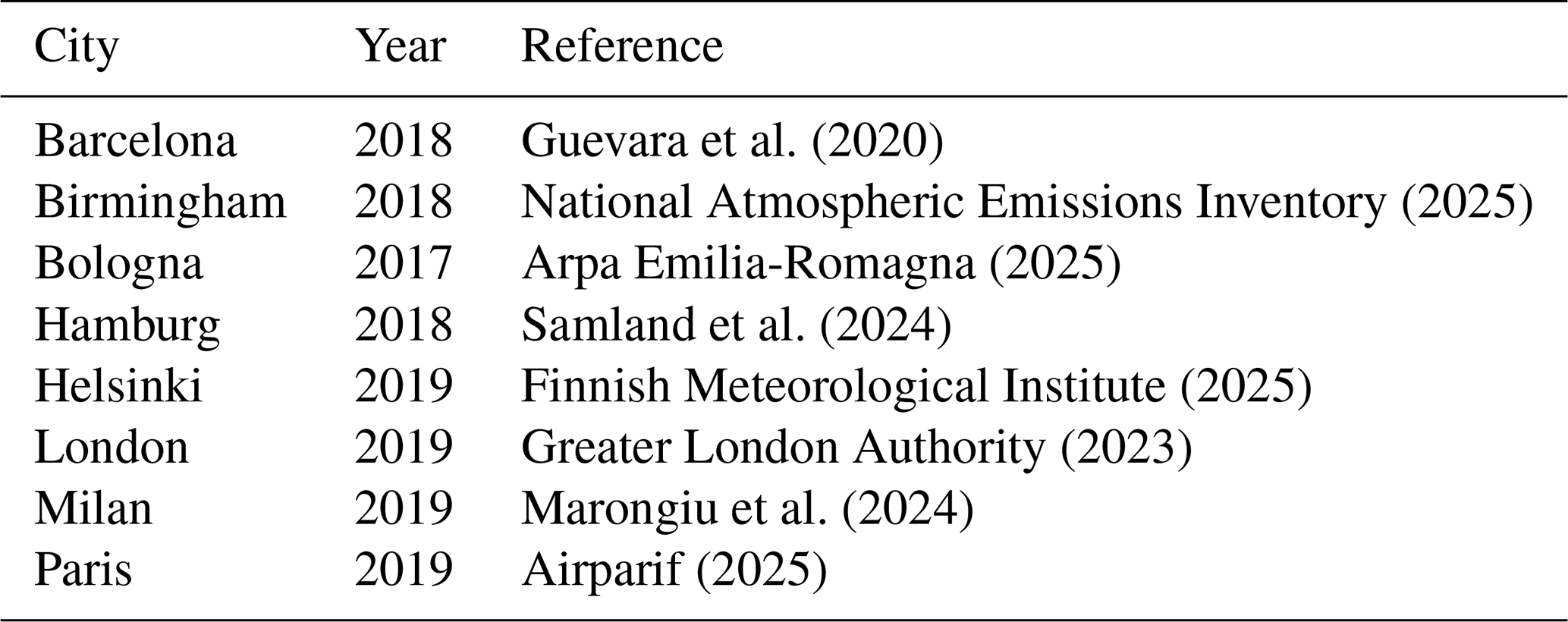
We used city-scale urban inventories independently generated by local or national authorities to compare our emission estimations on the local level, with the assumption that urban inventories incorporate the most detailed local information. Table 2 gives an overview of city scale inventories that were made available to us, for the sake of this comparison, by local authorities or institutes.

Guevara et al. (2020)National Atmospheric Emissions Inventory (2025)Arpa Emilia-Romagna (2025)Samland et al. (2024)Finnish Meteorological Institute (2025)Greater London Authority (2023)Marongiu et al. (2024)Airparif (2025)

Table 2 Summary on local NO_x inventories for road traffic used in this study.

2.2 Emission factors

For the calculation of NO_x emissions from road transport, this study used emission factors based on the Dutch national emissions inventory; for details and the full dataset, see Geilenkirchen et al. (2024). The methodology is vehicle-specific and uses a bottom-up approach introduced in 2019, which calculates emissions at the level of individual vehicles using annual odometer readings from the RDW (Netherlands Vehicle Authority). Each vehicle is assigned to one of approximately 350 VERSIT+ vehicle classes, defined by vehicle type, weight, fuel type, emission legislation category (i.e., Euro standards), and exhaust after-treatment technologies (Smit et al., 2007; Grange et al., 2019). Emission factors for NO_x are expressed in grams per vehicle kilometre and are road-type specific, distinguishing between urban, rural, and highway conditions. These emission factors are derived annually from both laboratory testing and real-world driving measurements, and are adjusted for vehicle aging using odometer data. NO_x temperature effects are not included in the Dutch national emissions inventory. Applying vehicle kilometres and vehicle type information from COPERT (Ntziachristos et al., 2009) to our emission factors dataset, we calculated the national emission totals for each country. In a next step, we derived weighted average emission factors per sector and vehicle kilometre. For this, the national emissions were divided by the total sector vehicle kilometres from COPERT. The COPERT dataset supplies yearly annual data on national vehicle fleet composition, and can readily be used to divide the dataset into relative shares for each vehicle category.

For each road link, the corresponding weighted emission factor was multiplied with the road's AADT value and road length. The weighted emission factor is dependent on the location (country) of the road, as well as the environment (urban, rural, highway) and vehicle class (see Sect. 2.2), resulting in an annual emission per year and vehicle class. In previous works, the urban–rural split was performed with gridded land use or population density data, resulting in all roads in an area sharing the same emission factors. However, emission factors of roads depend on the road conditions, maximum speed and congestion levels (Int Panis et al., 2006; Li et al., 2016; Franco et al., 2013), and not on the location of a road within an urban boundary. In an effort to choose the appropriate emission factor on a link level, we used urban emission factors for all roads with a speed limit of ≤50 km h⁻¹, and rural emission factors for all roads with a speed limit of >50 km h⁻¹. Maximum speed information was preferentially taken from OSM where available, or from OTM as a fallback. Highways were identified by road class and received their own emission factor independent of their speed limit.

The resulting dataset is referred to in Fig. 1 as bottom-up emissions. The term bottom-up emissions stands for the dataset which was based directly on our activity dataset. We then scaled bottom-up emissions with reported national totals (for more details, see Denier van der Gon et al., 2023) and gridded with 0.05° × 0.1° resolution to generate our final results for CAMS-REG v8.1 in line with the reported data. Both datasets aligned closely, with bottom-up emissions overestimating domain totals by 3 %.

2.3 Statistical methods

We used a combination of random forest (RF) models (see Sect. 2.3.1) and spatial gap filling (see Sect. 2.3.2) to create a complete dataset of AADT and maximum-speed values for most roads in the study area. This was done to generate a complete activity dataset. On this basis, the road-level emissions are calculated in a next step. Gap filling AADT data with machine learning approaches (Han, 2024; Sekuła et al., 2018; Razali et al., 2021) among them, random forest (Wen et al., 2022; Baffoe-Twum et al., 2023; Das and Tsapakis, 2020; Sekuła et al., 2018; Shen et al., 2024) is a common choice among traffic modellers, especially when working with mixed and incomplete data. AADT values were later used to calculate absolute NO_x emissions per road. A complete set of speed limits is necessary to choose the appropriate emission factor per road.

2.3.1 Random forest models

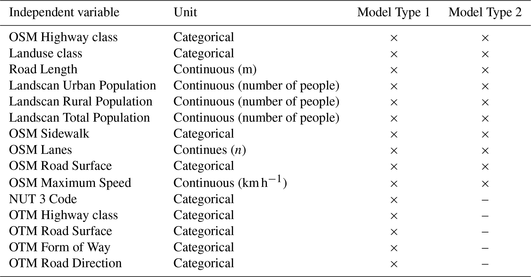
We first matched OSM road classes to their corresponding OTM class (Table 3). OSM links with road classes other than those given in Table 3 were ignored. Subsequently, RF models were trained to predict AADT values for OSM links without available AADT data from OTM. After initial testing, we noticed that a single RF model over all modelled road classes resulted in larger model errors for high-intensity highways; therefore, we trained an additional highway model, predicting only for missing highway links (Table 3). Information on road class and speed limits from the OTM dataset, as well as land use data from CORINE, was not available for the previously outlined non-EU Eastern European countries. For the use in these locations, we trained RF models that excluded these variables. In total, we thus trained four different RF models, differentiating between highway/non-highway as well as OTM data availability. These models are called RF model 1 (for non-highway roads in EU countries), RF model 2 (for non-highway roads in non-EU countries), RF highway model 1 (for highways in EU countries) and RF highway model 2 (for highways in non-EU countries). An overview is given in Table 3. An overview on the independent variables used in both model types is givein in Table 4.

Table 3 Matching table between OSM and OTM classes and gap filling approach used. Model 1: Model includes OTM predictors. Model 2: Model excludes OTM predictors, for use in non-EU countries.

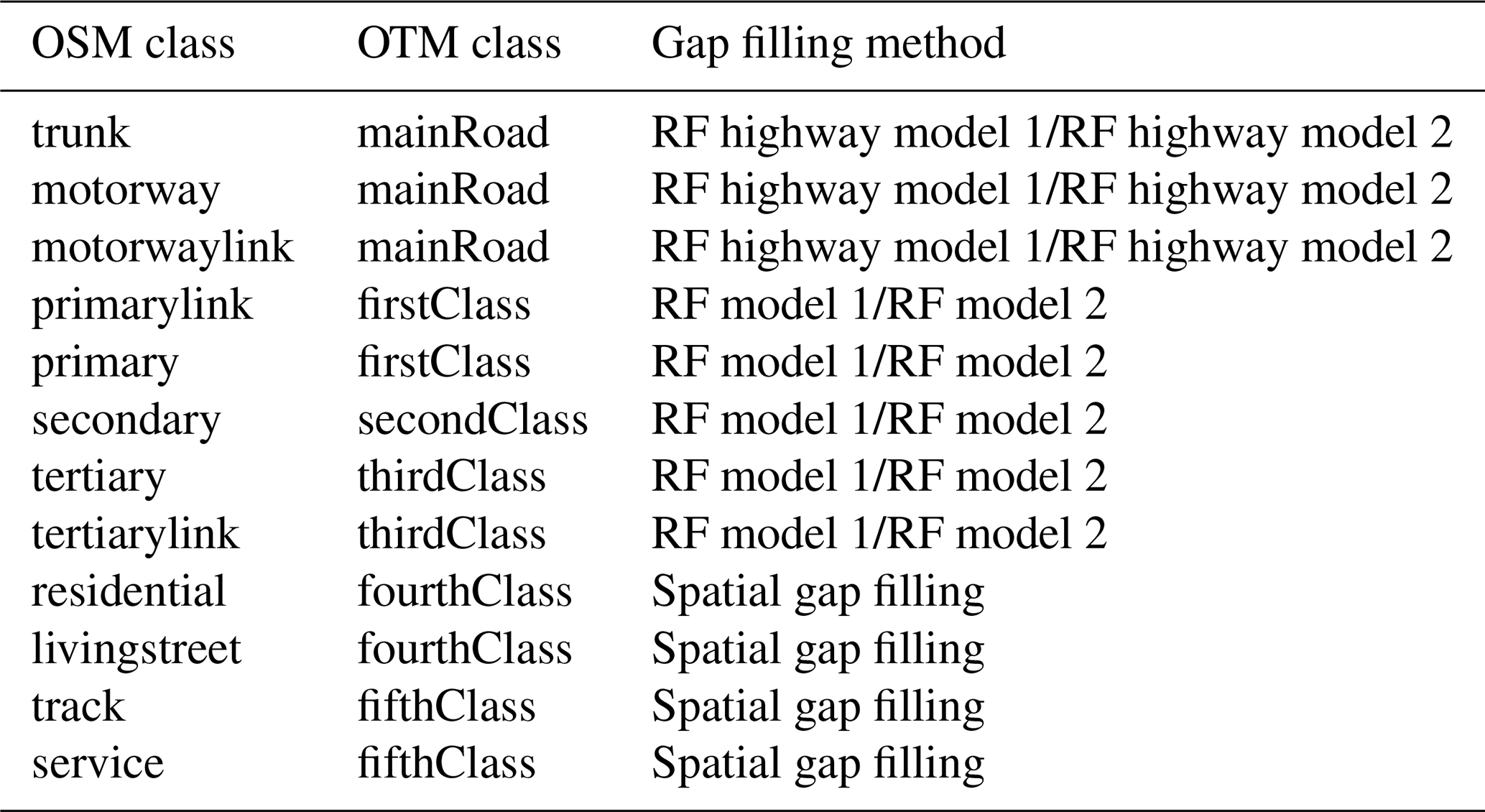
Table 4 Overview on predictors used for Model Types 1 and 2. Model 1: Model includes OTM predictors. Model 2: Model excludes OTM predictors, for use in non-EU countries.

For RF modelling, we used the randomForestSRC library (version 3.3.1) (Ishwaran and Kogalur, 2024). The number of trees was set to 250 trees per model, with 10 % of data reserved for testing. All other settings were kept to the library defaults. Missing predictor data was handled by imputation with random forest (for details see Ishwaran and Kogalur, 2024).

The maximum speed of each link was used to decide whether to use urban (<50 km h⁻¹), rural (50–100 km h⁻¹) or highway emission factors (>100 km h⁻¹) in the case were a straightforward identification by road class was not possible. We first categorized all fourth- and fifth roads key as urban, and all mainRoad, motorway and highways (OTM classes) as highway. For other road classes, information on maximum speed was taken from OSM and OTM data where available, with a preference for OSM data, as this information came from a more recent dataset. Then, all maximum speed data were transferred into the three outlined categories. Subsequently, one RF model with the above mentioned settings was trained to predict these categories for all links missing maximum speed information.

2.3.2 Spatial gap filling

For local roads (forth and fifth class roads), no information on traffic volume was available from OTM. In our dataset, these local roads account for 79.1 % of the total road length, and it was thus seen as important to also estimate AADT values for all local roads, even if the traffic volumes were expected to be low for each road. For these roads, we used a gap filling approach based on the average traffic volume of tertiary roads in the surrounding area (see Table 3). Approaches for estimating local road data in the literature include regression approaches (Apronti et al., 2016; Pulugurtha and Mathew, 2021; Sun and Das, 2015), spatial techniques such as kriging or inverse distance weighting (Baffoe-Twum et al., 2023) or machine learning approaches (Baffoe-Twum et al., 2023; Sharma et al., 2001). After performing gap filling for larger roads using our RF method (Sect. 2.3.1), we divided the study area into 5 × 5 km grids, and removed the top 25 % of tertiary roads with the highest traffic volume within each grid cell to handle outliers. Removal of the top quantile was done due to a number of third class roads carrying a very high traffic load (for example highway exits), which were deemed less relevant for the prediction of residential roads. Then, we took the mean of the remaining tertiary roads' traffic volume within each cell. The traffic volume of fourth- and fifth class roads were set to 30 % and 15 % of that value, respectively, resulting in a minimum AADT of 15 for fourth class roads, and a minimum AADT of 8 for fifth class roads. Macbeth (2007) give the ratio of typical values between urban collector (which maps to our third class roads) and local roads to around 30 %. Cornell Local Roads Program (2014) give a typical cut off between low- and high volume roads at an AADT of 1000. Further, the cut off between low- and very-low volume roads is given at around 400. Our judgement on reasonable percentage-base values for forth- and fifth class roads was made based on these sources.

The resulting raster values used to estimate small roads' AADT ranged from 50 to 3358, with a mean of 57. This results are comparable with estimations from previous studies (Pulugurtha and Mathew, 2021). The smaller roads on which spatial gap filling was performed result to less than 4 % of total domain emissions (see Table 1). Therefore, the spatial gap filling method does not have a large effect on domain totals.

2.4 Comparison to CAMS-REG v4.2 method

Based on the introduced methodology and datasets, CAMS-REG v8.1 includes the first major update on the spatial distribution of road emissions since v4.2, which was published in 2022 (Kuenen et al., 2022). At the core, both methods are based on the activity data distribution from OTM in combination with OSM shapes and a methodology to fill up missing data (see Fig. 1). In v4.2, the link-based activity data is first filled up by taking an average of the road type within each corresponding NUTS3 area, or, if not available, a global average. Then, emission factors from COPERT were applied, and the spatial distribution was gridded to a fixed grid of 0.05° × 0.1° resolution. Lastly, empty grid cells with no available data; for example in non-EU Eastern European countries were filled up using a regression approach based on Landscan population density data, per road class. The resulting spatial dataset was then used to distribute national total emissions per country.

The spatial distribution, as well as large parts of the data handling within this version, is dependent on the exact grid definition, and an increase of grid resolution is not possible beyond the resolution of Landscan for large parts of the study area. If city scale or higher resolution inventories need to be derived from this approach, additional tools and proxies are always necessary. So far, this has been done by either tools such as UrbEm (Ramacher et al., 2021), or proxies such as local road geometries or other distributions.

2.5 Evaluation methods

Here, we describe the evaluation of our intermediate results and the final dataset.

RF gap filling model performance was tested with 10 % reserved test data and the coefficient of determination (R²), mean absolute error (MAE) and root mean square error (RMSE) as performance metrics.

Due to the scaling with national emission totals (Fig. 1), national totals of the final emission datasets are bound to be similar to previous versions on a national level, despite the base year difference of 2017 (v4.2) and 2018 (v8.1). National totals used to scale emissions for the two CAMS-REG versions used may be slightly different due to updates in the national methodologies.

We then compare our results to the 8 made-available city scale inventories (see Sect. 2.1.4). For this, the boundary shapes of the city inventories were used to extract annual emission totals from CAMS-REG versions, which were then compared to the city inventories. The areas of these boundary shapes included regions of different sizes, which are available as described in Sect. 4. The largest city boundary was for the Paris-Ile de France region (ca. 12 470 km²).

For a wider picture, we included 16 other European cities for a comparison between CAMS-REG versions. As different national totals between the CAMS-REG versions can also affect city allocation, comparisons were also done on a “Share of urban emissions to national totals” basis.

For London and Milan, in addition to city totals also a high-resolution spatial distribution is available from LAEI and ARPA Lombardia, which enables a case-study comparison of the spatial distribution between different methods. We gridded our new distribution to grid of the local inventory, and performed an UrbEm downscaling of CAMS-REG v4.2 to the same grid. We then performed a spatial correlation between the local inventory and both CAMS inventories, as well as spatial cross-correlation. Spatial cross-correlation has been proposed by Chen (2015) as a way to assess the relationship between one variable at a location and another variable at other locations. It is an extension of the commonly used Moran's I index for spatial autocorrelation over another variable (Chen, 2015). Possible values reach from −1 to 1, with −1 denoting perfect negative cross-correlation, 1 denoting perfect positive cross-correlation, and 0 denoting no cross-correlation.

3 Results

In this section, we give the performance of the trained AADT models. The gap filling of AADT data is done with the aim of generating a complete activity dataset for the later emission calculation. The unit of AADT is vehicles per day. In the following, we give an overview on the resulting emissions dataset. We then compare the total results with emissions from local inventories. We further included a comparison of the spatial distribution of local inventories for London and Milan inventories against CAMS-REG.

3.1 Model performance

RF Gap filling performance was dependent on model and road type. Model 2 (see Table 3) reaches R²=0.63, whereas Model 1 (trained also with OTM data) reaches R²=0.74. This performance decreases along decreasing road size, with primary roads achieving R²=0.64, secondary roads R²=0.51 and tertiary roads R²=0.44 for Model 2 and R²=0.47, R²=0.39 and R²=0.29 for Model 1, respectively. The MAE and RMSE for Model 2 are MAE = 2028.3 and RMSE = 4407.2. Errors increase with road class (highway MAE = 5182.3, tertiary roads MAE = 619.7). For the Model 1, errors were MAE = 1570.2 and RMSE = 3702.4.

For motorways, the highway models achieve R²=0.66 and R²=0.76 for Highway Model 2 and Highway Model 1, respectively (see also Fig. 2).

We further calculated variable importance according to Ishwaran and Lu (2019). For Model 2, the most important predictor variables were the OSM highway key, and then population density and land use class. For Model 1, the OTM road class was the most important predictor, followed by population density and the OSM highway key. For both models, OSM data on maximum road speed were of low importance.

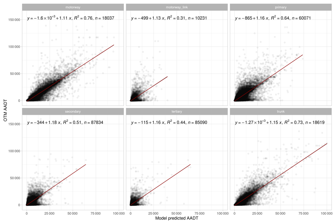
Figure 2 Performance of RF AADT–gap filling model 1 (for use in EU countries), by road class for the year 2018.

3.2 Validation of activity dataset with measured dataset

We compared our complete activity dataset to a recent dataset published by Bonnemaizon et al. (2025). This dataset provides measured, annual averaged traffic data for a number of European cities between 2015 to 2024 depending on availability. The locations of traffic counts were matched with the OSM network by Hidden Markov Models (in case of line geometries) and nearest neighbour approach (in case of point data). The performed matching with the OSM network provided a straightforward way for comparison with our dataset.

For the year 2018, data was available for 13 cities, for a total number of 6219 traffic counting stations. The number of stations per city varied strongly, with the smallest number in Copenhagen (n=17) and the largest number in London (n=2207). Motorways (motorway + trunk) accounted for 1056 stations, primary (primary + primary_link) for 1570 stations, secondary (secondary + secondary_link) for 825 stations, tertiary (tertiary + tertiary_link) for 1217 stations and residential (residential + service + living_street) for 1430 stations. Descriptive statistics were (min: 5; 25 % quantile: 3775; median: 10 288; mean: 15 405; 75 % quantile: 18 530; max: 163 045), compared to our generated dataset: (min: 0; 25 % quantile: 221; median: 1449; mean: 4508; 75 % quantile: 3841; max: 107 656). Frequent high values for residential streets in the dataset from Bonnemaizon et al. (2025) hint to a possible mismatch of some sensor locations. For example, the mean AADT of service roads was 21 572, which is likely be explained by a location mismatch. Bonnemaizon et al. (2025) are aware of this source of error.

Correlation between both datasets was found at R²=0.17, p<0.01 with a slope of b=0.84. Bonnemaizon et al. (2025) mention higher certainty of their matching algorithm with reduced distance between sensor and matched roads. We therefore performed the analysis again in two steps. First, we only took into account sensors with matched roads close to the sensor location (distance < 1 m; n = 3476), as suggested by the authors to help reduce matching uncertainty. Secondly, we only took into account sensors that came with a matched line geometry, increasing location certainty even further (n=2249). In the first case, correlation increased to R²=0.20, and in the latter case to R²=0.38, which is still below R²=0.5, a value seen satisfactory by Bonnemaizon et al. (2025). Our RF gap filling methodology did not seem to negatively impact correlation with the validation dataset. Using only gap filled data, correlation increases from R²=0.17 to R²=0.27.

The statistics show a large underestimation in our dataset. The underestimation is the largest for small roads (by factors of 210 for service roads and 18 for residential roads, with likely reasons as outlined before). Amongst other road classes, there is an underestimation of our dataset by a factor ranging from 2–6 for different per road class. As road traffic volume in Europe still generally continues to grow (EEA, 2024), a part of the underestimation may be explained by OTM's 2015 base year compared to the measured data from 2018. However, there seems to exist an additional systematic underestimation of AADT values in the OTM dataset for urban areas compared to the measured data.

Our findings of a substantial increase in correlation with decreasing geolocation uncertainty is in line with previous results by Bonnemaizon et al. (2025), who explain weak correlation with a validation datasets due to uncertainty in geolocation of sensor data. For the final purpose of generating a relative spatial distribution, the low correlation values between between our dataset and the measured data are a limitation to our results, highlighting the need for an updated and consistent AADT dataset in Europe.

3.3 Resulting emissions and datasets

As absolute emissions per country were scaled by reported country totals, emissions on the country levels between CAMS-REG versions differ only due to changes in country reporting methodology for a given year. Figure 3 gives an overview of changes in country totals. The NO_x domain total for CAMS-REG v4.2 was 3.67×10⁹ kg, and 4.03×10⁹ kg in v8.1 for 2018. The largest absolute increases in reported emissions were for Turkey and Russia and the largest decrease, for Poland. We further calculated the changes of urban core emissions between the versions. Urban core areas were taken from the Global Human Settlement Layer (Pesaresi et al., 2024). Throughout the domain, urban emissions increased by 26 %. Large increases can be found in non-EU countries such as Georgia, Russia, Serbia and Turkey (Fig. 4). Strong decreases can also be found, for example in Estonia and Finland, which occur due to the spatial redistribution of emissions.

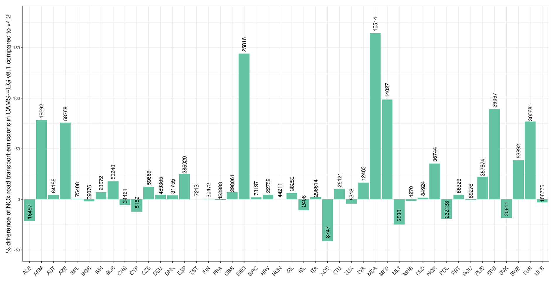
Figure 3 Percentage difference of NO_x emission estimations between CAMS-REG versions 8.1 and 4.2 for the year 2018. Positive values denote higher estimations in version 8.1. Labels are absolute emissions (t yr⁻¹).

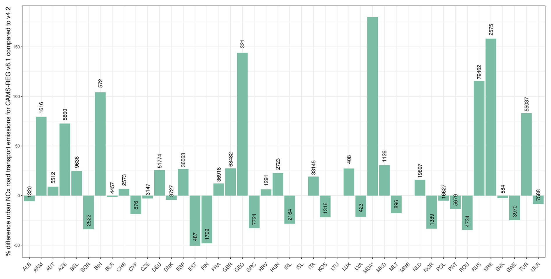
Figure 4 Percentage difference of urban NO_x emission estimations between CAMS-REG versions 8.1 and 4.2 for the year 2018. Positive values denote higher estimations in version 8.1. Labels are absolute emissions (t yr⁻¹). ^* We cut the value for Moldova (MDA) to preserve scale (409 %).

A distribution of absolute emissions by OSM class is given in Table 5. Over 65 % of all emissions occurs on trunk, motorway and primary roads, with another roughly 15 % of emissions occurring on secondary and tertiary roads. Despite their large number, smaller roads only account to 3.7 % of all emissions in the domain.

Table 5 Distribution of absolute and relative shares of NO_x emissions in the domain by OSM class.

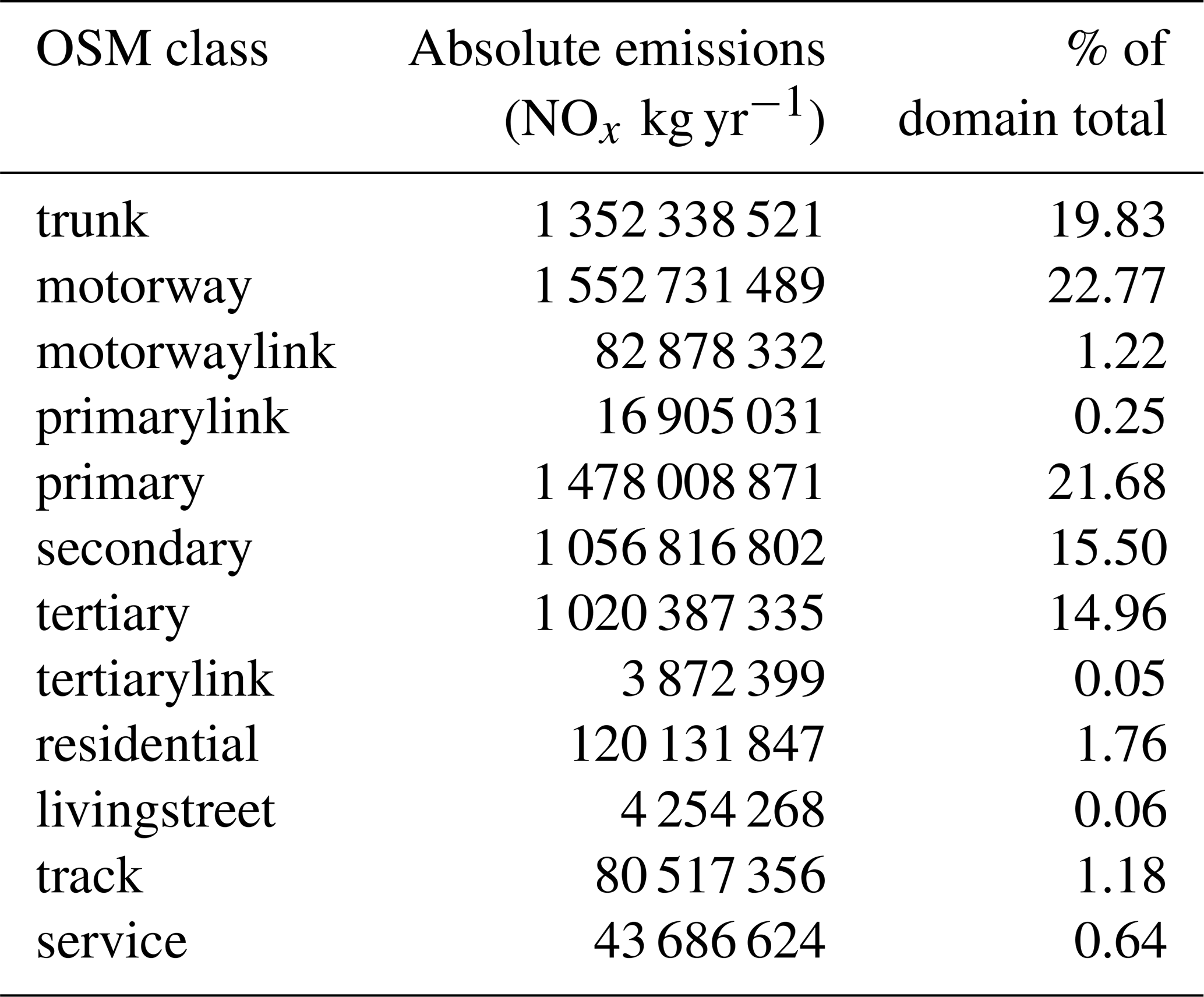
Figure 5 gives an overview of the spatial distribution for France, Russia and Ukraine. France shows a higher allocation to urban centres, with a largely unchanged spatial distribution for the rest of the country. Russia and Ukraine show vastly different spatial distributions, with more emissions attributed to cities, visible urban centres and highways, as well as a reduction in artifacts.

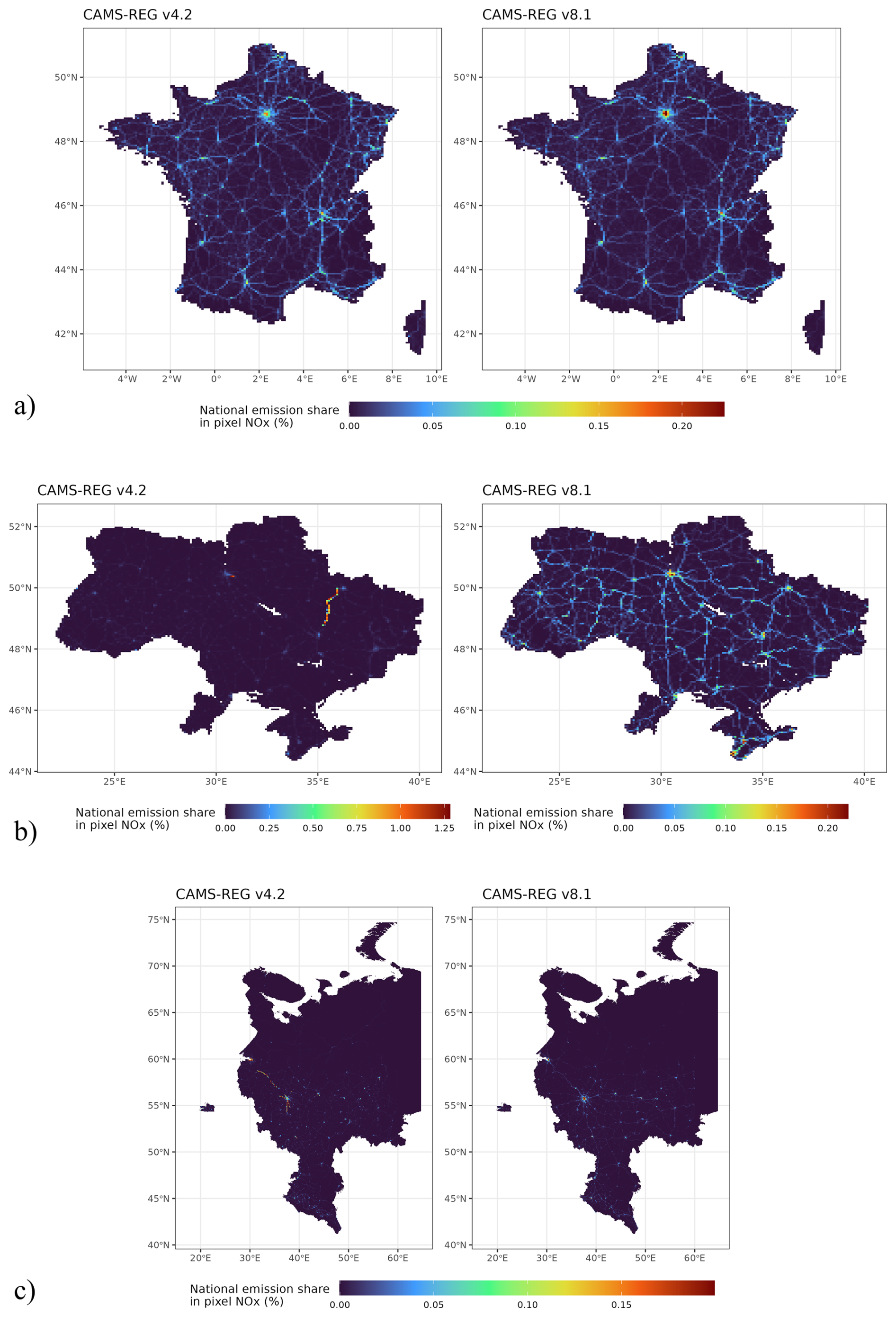
Figure 5 Spatial distribution of road emissions for France (a), Ukraine (b) and western Russia (c) between CAMS-REG versions 4.2 and 8.1. Please note the different colour scales on the left and right side plots of (b).

3.4 Comparison with city inventories

As city inventories compiled by local institutes or authorities are prepared with the most detailed local knowledge, they are here seen as the gold standard with which to compare our European emission dataset. Nonetheless, there could be also significant errors in the spatial distribution and absolute emission estimates of local city inventories. We compared the absolute NO_x estimations for CAMS-REG v4.2 and CAMS-REG v8.1 to the data of eight cities for which independent city inventories was made available to us (Sect. 2.1.4).

Absolute emission comparisons are given in Fig. 6. The mean absolute percentage error of CAMS-REG v4.2 in comparison with local city inventories was 35 %, with the smallest error for Paris (18 %) and the largest error for Bologna (53 %). All cities showed underestimations in CAMS-REG v4.2 compared with local inventories, which we explain by the generally too-low urban AADT values from OTM-based estimation (Sect. 3.2), as well as the more basic gap filling approach employed in v4.2.

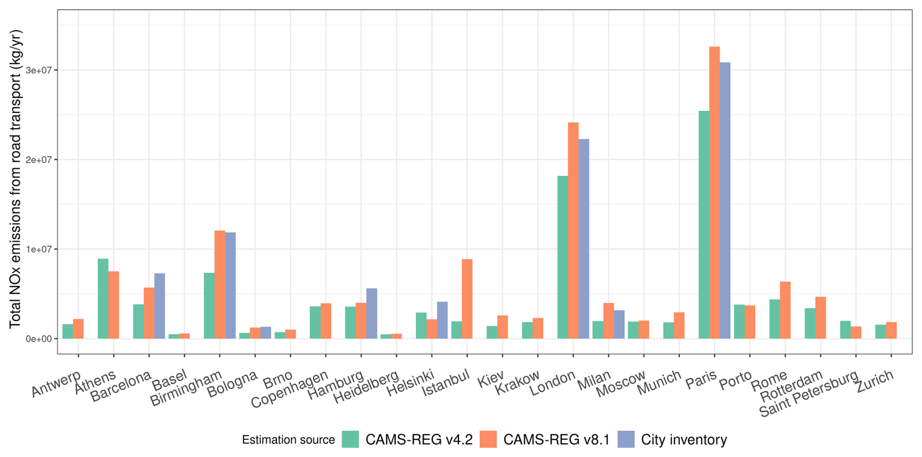
Figure 6 Comparison of annual NO_x emissions from road transport of CAMS-REG 4.2, CAMS-REG 8.1 and local city inventories for 2018. Years covered by local inventories are given in Table 2. Note that the areas covered by city boundary shapes vary substantially. The city boundaries used for this comparison are provided in Sect. 4.

Using CAMS-REG v8.1 emissions, the average difference was 18 % compared with the city scale inventories. All estimates improved except for Helsinki, and improvements were largest for Barcelona and Milan. CAMS-REG v8.1 largely underestimates emissions for Helsink (−26 %), and overestimates emissions for Milan (+26 %).

Higher emission totals in urban areas were also estimated for most of the cities for which no locally-made city inventory was available for comparison (see right side of Fig. 6). Here, Kiev and Istanbul saw strong increases compared to CAMS-REG v4.2 (+84 %, +360 %, respectively).

Absolute emission estimates are impacted not only by the spatial distribution of country totals, but also by the country totals themselves. Between CAMS-REG v4.2 and v8.1, there has been a change in reported country totals for some countries (see Sect. 3.3). To understand the separate effects of the spatial distribution, we compared the relative shares of urban NO_x emission to country totals between both versions (Fig. 7). Here, the relative shares of urban emissions increased for most cities, with the exception of Helsinki, Athens and Porto. The case of Helsinki is the only city showing a decreasing performance compared to the local inventory. In CAMS-REG v4.2, a large proportion of Finnish national emissions were allocated to the capital city (Fig. 7), in line with the population-based method used (Sect. 2.4). In Finland, over 30 % of the population lives in Helsinki, which is a high value for Europe (Eurostat, 2024).

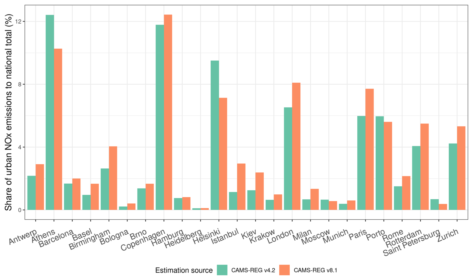
Figure 7 Share of NO_x urban emissions to national totals between CAMS-REG versions 4.2 and 8.1 for road transport in 2018.

The absolute emission changes in each city follow the changes of relative urban emission shares (Figs. 6, 7). Therefore, the changes between CAMS-REG versions can be attributed to the updated spatial distribution. Across all cities, the mean increase of urban emission share was 34 %. Istanbul, Milan and Kiev saw high increases of relative shares (160 % and 100 %, 90 %, respectively) (see Fig. 5).

3.5 Spatial distribution London

Figure 8 compares the spatial distribution for London between the urban inventory (LAEI) and the previous and recent CAMS-REG estimates in 1 × 1 km resolution, normalized by total urban emissions. The original 0.05° × 0.1° resolution of the CAMS-REG v4.2 dataset was downscaled to 1 × 1 km using the UrbEm tool (Ramacher et al., 2021). In the local and CAMS-REG v8.1 estimates, major roads such as the outer M25 ring or the North Circular Ring are clearly visible. Compared to the local inventory, CAMS-REG v8.1 seems to overestimate emissions at certain highways. Spatial correlation between the local inventory and CAMS-REG v8.1 reaches R²=0.62, with p<0.001, and spatial cross-correlation was calculated at I=0.06, p<0.001. Spatial correlation between the local inventory and CAMS-REG v4.2 reaches R²=0.33, with p<0.001 (downscaled with UrbEm), and spatial cross-correlation at I=0.11, p<0.01. Spatial autocorrelation of the local inventory (Moran's I) is I=0.07.

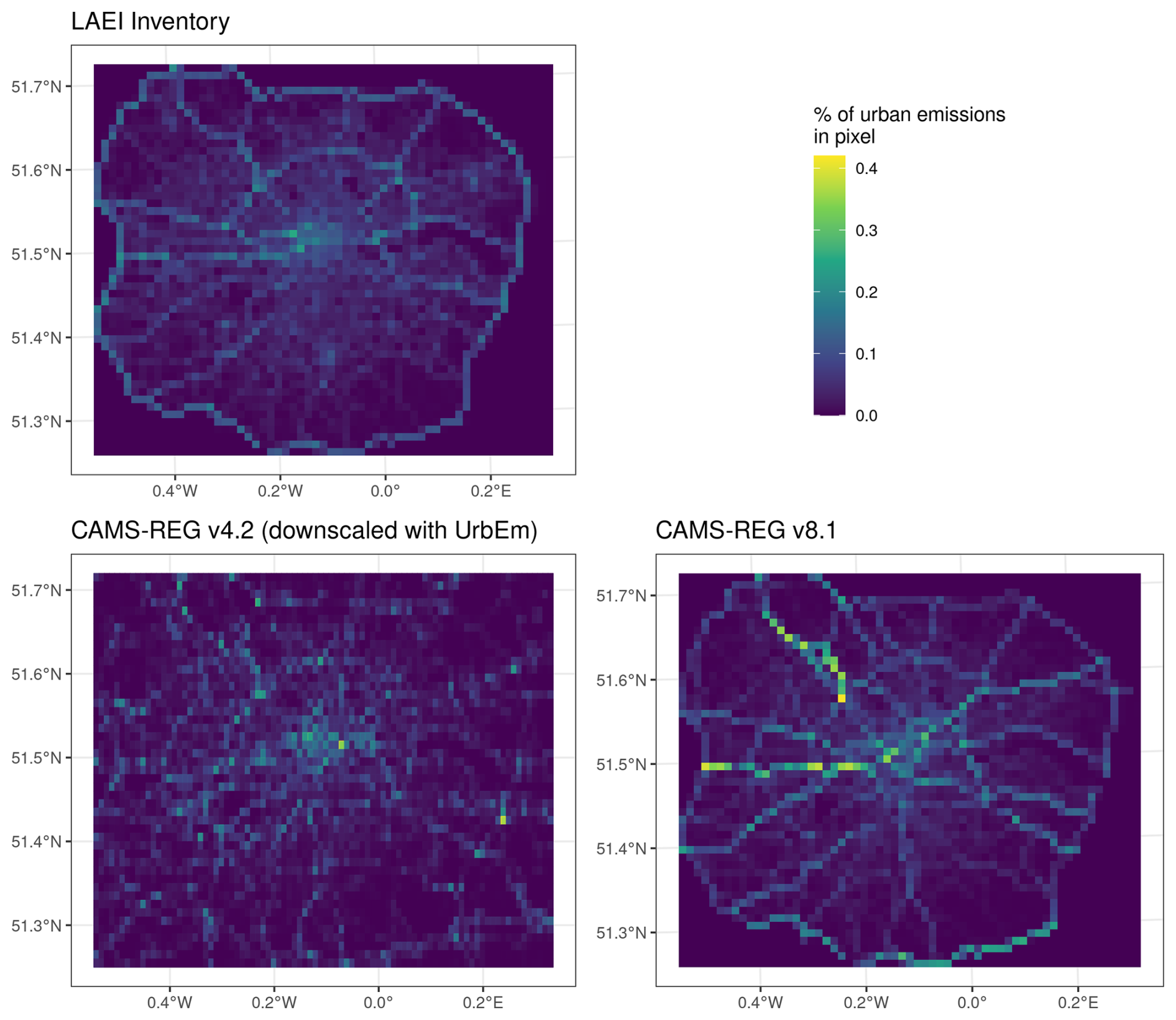
Figure 8 Comparison of the spatial distribution of urban NO_x road transport emissions for London with local (LAEI, base year 2019) and CAMS-REG inventories (1 km resolution, base year 2018).

3.6 Spatial distribution Milan

To derive a local inventory for Milan, Marongiu et al. (2024) started with a complete road graph that had been simplified to include the fewest oriented arcs capable of representing the most significant motions. Data from motorway companies, ANAS (National Autonomous Roads Corporation) and local authorities of vehicular traffic data (from traffic counters, cameras, passages at toll booths and motorway barriers) were used in a flow assignment model for estimating the origin and destination matrices over the entire network. To extend the spatial extension of the detailed estimates and avoid the calculation of diffuse traffic emissions, the simplified road graph was used to train and test (with a data split of 75 % and 25 %) a RF model for predicting emissions by road arch, according to the following variables: vehicles (cars, high-duty, low-duty and motorcycles) and 12 variables describing road characteristics. The ML performances are confirmed for training and testing in the range of an R² of: 0.8–0.6 for high duty, 0.9–0.8 for light duty, 0.8–0.7 for motorcycles and 0.9–0.7 for passenger cars. For a detailed description of the Milan local inventory, see Marongiu et al. (2024).

An overview of the spatial distribution of road transport emissions from the local Milan inventory and CAMS-REG versions are shown in Fig. 9. Like to London, the CAMS-REG v4.2 inventory was downscaled using the UrbEm tool to match the spatial resolution of the local inventory. The Milan local inventory places most emissions on the outer ring road of Milan, while also estimating emissions for small roads. CAMS-REG v8.1 places more emissions on the inner ring road, and less emissions on local roads in general. Ring roads and highways are less visible in CAMS-REG v4.2. Spatial correlation between the local inventory and CAMS-REG v4.2 (downscaled with UrbEm) inventories reaches R²=0.25, with p<0.001, and spatial cross-correlation is at I=0.08 with p<0.001. The spatial correlation between the local inventory and CAMS-REG v8.1 is R²=0.59, with p<0.001, and spatial cross-correlation reaches I=0.06 with p<0.001. Moran's I (spatial autocorrelation) for the local inventory is at I=0.07. Low spatial autocorrelation is captured in both versions of CAMS-REG.

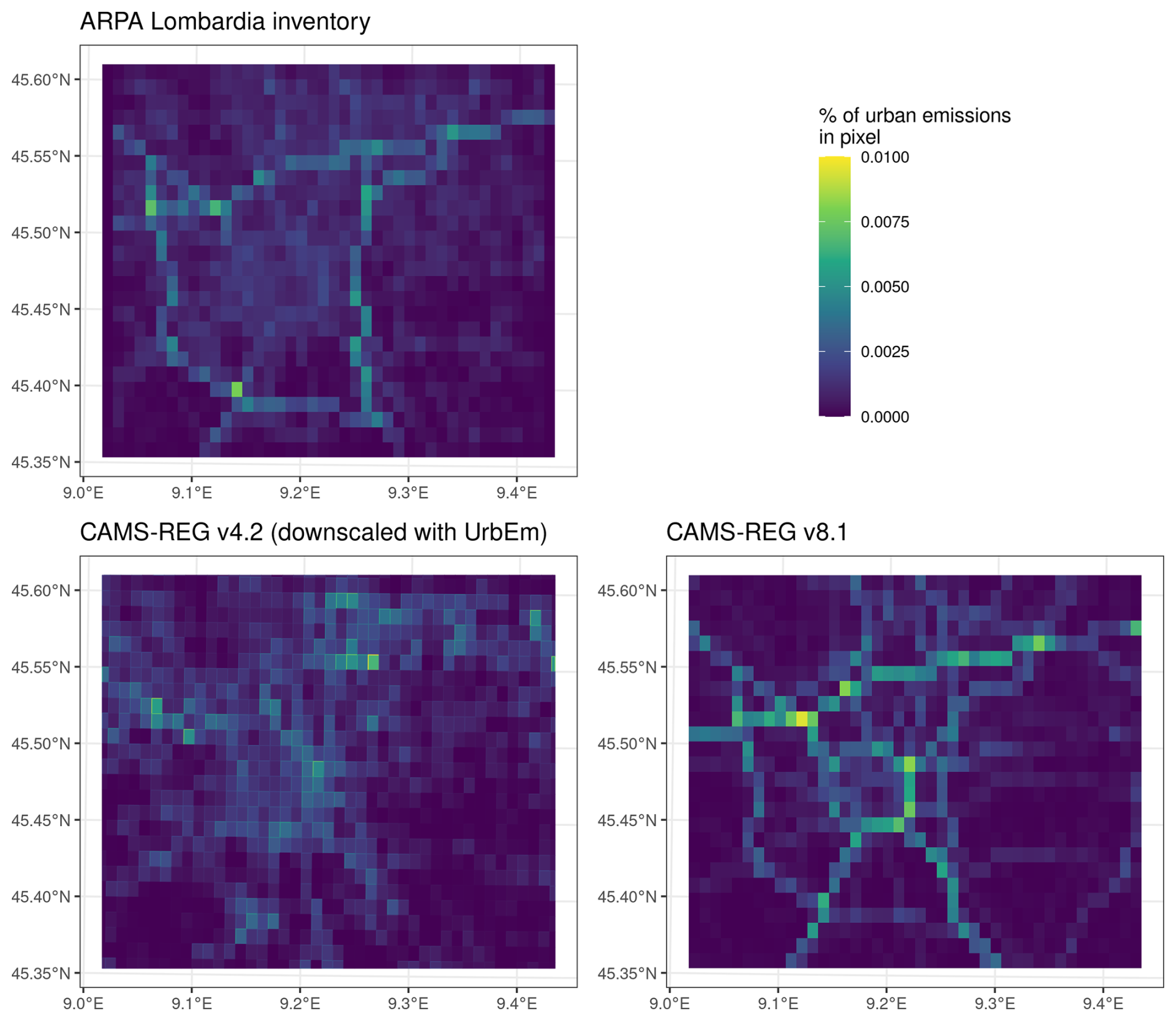
Figure 9 Comparison of the spatial distribution of urban NO_x road transport emissions for Milan with local (base year 2019) and CAMS-REG inventories (0.01° × 0.007° resolution, base year 2018.

3.7 Comparison between speed-based and land-use–based allocation of urban and rural roads

Our emission factor set differentiates between urban roads, rural roads and highways. The allocation to highways was straightforward, and is done via OSM classes (see Table 3).

We further tested the impact of the methodology to determine whether a road receives an urban or rural emission factor. In the previous version of this dataset, the emission factor of roads (or of gridded road proxies) was determined by land use class or population density (Kuenen et al., 2022). In this update, we set the road status by the maximum driving road speed allowed on the road (see Sect. 1). This was thought to better represent real-world emission factors than the land use class around the road and align the method with the approach of the COPERT emission inventory model (Ntziachristos et al., 2009). For the first method, we gave an urban status to roads within an urban CORINE grid cell (CORINE categories 1.1.1 or 1.1.2). For the second method, we attributed urban status for roads with a maximum speed of ≤50 km h⁻¹.

Figure 10 shows a comparison of urban and rural allocation for both methods. It is visible that the allocation by maximum speed leads to more emissions being classified as urban, both inside and outside urban areas. These roads subsequently receive urban (and therefore higher) emission factors compared to rural roads. Over the whole domain, the ratio of urban to rural emissions is greatly different for both approaches. Using a speed-based approach, the ratio between urban and rural emissions is approximately 4 : 1, whereas it is approximately 1 : 2 when using a land-use–based approach. This leads to a wider use of higher, urban emission factors in the speed-based approach (see Fig. 10). We tested the impact of both methods on overall city emissions (Sect. 3.4). For each city, the difference was very small and typically less than 1 % of the final result.

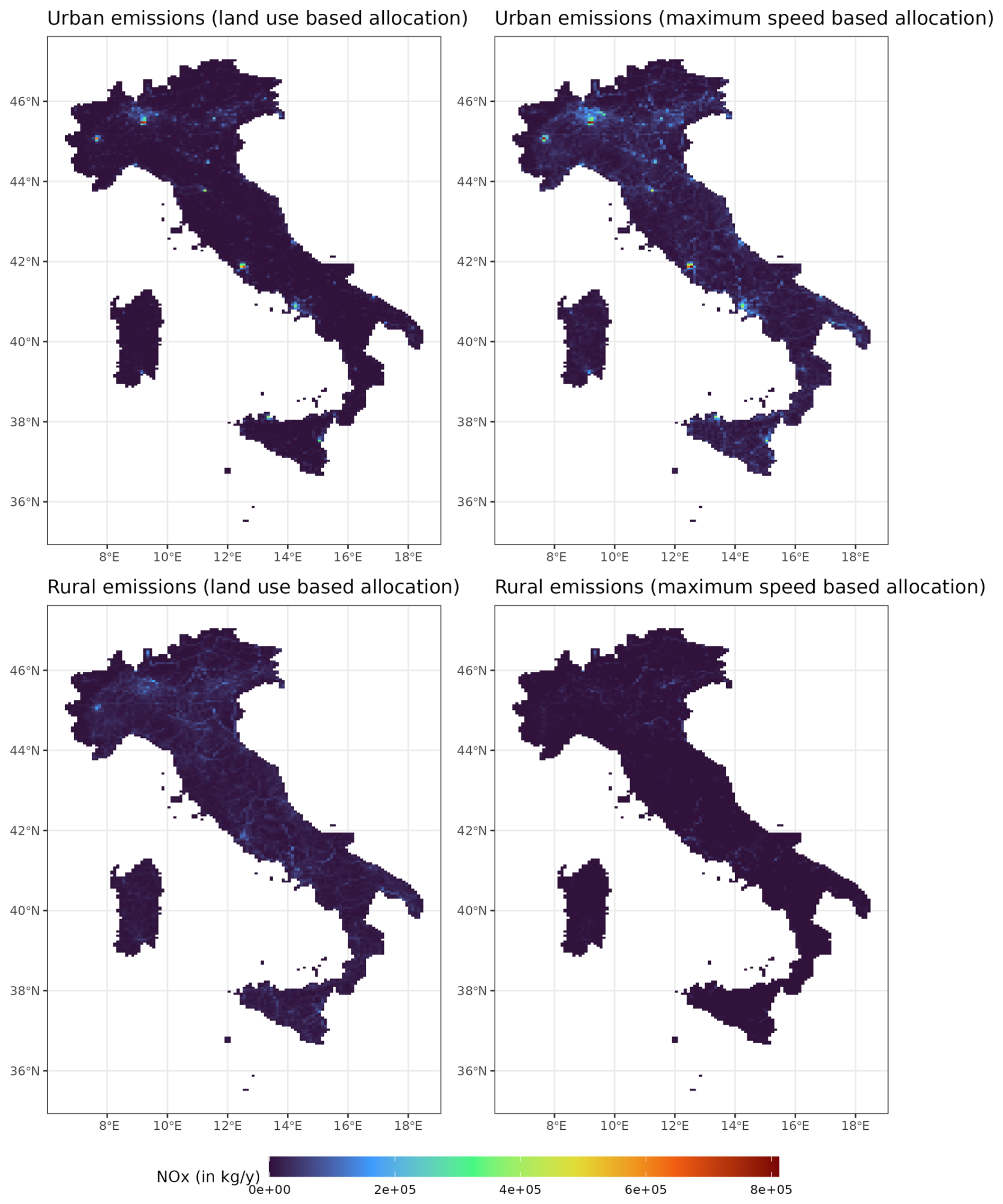
Figure 10 Comparison between speed-based and land-use–based urban/rural distinction for Italy for 2018.

4 Data availability

Data is available in vector format and gridded raster format at a resolution of 0.05° × 0.1°. The vector dataset includes all information necessary to derive a gridded spatial distribution for different resolutions and extents. Fields include traffic volume, road class, road length, country code, urban/rural/highway category, and total emissions per vehicle type, as well as total vehicle kilometre per vehicle type. The raster dataset is gridded per vehicle type and urban/rural/highway category. Moreover, the city boundary shapes used to compare local and CAMS-REG inventories are included. Detailed information on each field of the vector file are given in an included Readme file.

Data can be found at https://doi.org/10.5281/zenodo.15688722 (Hohenberger et al., 2025).

5 Conclusions

This study presents a new spatial distribution for road transport emissions in Europe to improve CAMS-REG emission inventories. The motivation for a new spatial distribution was three-fold. Firstly, comparisons with urban inventories showed frequent underestimations of urban NO_x emissions by CAMS-REG v4.2. Secondly, work-intensive methods such as the use of downscaling tools or urban proxies had to be employed to create urban inventories with high resolutions needed for detailed exposure studies or urban air quality management (Venter et al., 2023; Gulia et al., 2015; Yang et al., 2019) from existing emission inventories. Thirdly, spatial distributions for countries in Eastern Europe were faulty and suffered from artifacts due to the lack of available data. To overcome these challenges, a vector-based methodology was applied, in which emissions are calculated for all roads on a link level first, and then flexibly gridded to the required resolution. A major part of the work was the gap filling of missing activity data to create a coherent dataset. This was done using random forest models and OTM, OSM with land use and population density data, and a spatial approach for the smallest roads. Comparing the resulting dataset to independent city inventories revealed an improved NO_x emission allocation in seven out of eight cities for which data was available, and an allocation of emissions to non-EU Eastern European cities comparable to their EU counterparts. Case study comparisons of spatial distributions in London and Milan lead to similar results. Compared at an approximately 1 km scale, in both cases spatial correlation increased from around R²≈0.3 using CAMS-REG v4.2 and UrbEm downscaling to R²≈0.6 with CAMS-REG v8.1. As the random forest models rely on OSM data for training (for example for road class information) as well as for road geometries, the community character of OSM is introducing an uncertainty source. Even though OSM data has been found reliable in previous studies (Demetriou, 2016; Moradi et al., 2021), we found the data availability of attributes low, and different units (mph and km h⁻¹) in maximum speed data needed to be translated, with possible error room for different labelling conventions.

We trace the previously too-low allocation of emissions to urban centres back to the incomplete and more simple gap filling performed in CAMS-REG v4.2. Here, a larger share of emissions was attributed to highways, as their data availability was higher. The complete estimation of activity data, which now also includes small roads, led to the increase of urban emission allocation and a better comparison with urban inventories. Section 3.7 further shows a largely different ratio of urban and rural emissions based on the allocation method. As all emissions were scaled by national totals, this did not change overall emissions, but also contributed to a higher share of emissions within city centres. When using land-use–based methods, we found a proportion of urban centres outside urban categories (Corine code 1.1.1 or 1.1.2), leading to a likely misallocation of roads. Further, higher emission factors were strictly limited to urban centres, even though many roads in rural areas may also be operated on with low speeds or high congestion levels, which will lead to higher emissions for these roads (see Kelly, 2025; Li et al., 2023 for related research).

The selection of emission factors for road links based on speed limit or congestion status is seen as an important step towards an improved spatial distribution.

For consistency with previous CAMS-REG versions, we based our approach on the OTM dataset, which has also been used in CAMS-REG v4.2 as the main source of activity data. The OTM dataset was published in 2016, after the use in a number of pilot regions as part of the EU-funded Open Transport Net project (Jedlicka et al., 2016). The results could be improved by the addition of more and more up-to-date datasets. These could be integrated based on their OSM-ID in a hierarchical fashion, in which measured and newer data takes precedence over modelled or older data, while taking care to produce a harmonic dataset. This integration work will be a major task for the future.

The published dataset is to our knowledge the first attempt to provide coherent vector-based road emissions for most roads in Europe, which can be gridded in any resolution to serve as a base for detailed urban air quality analysis and exposure studies. The dataset can be used in cities to provide a starting point for their own work on an inventory and as a reference point for comparison, which will help to improve our estimates as well. Future work is planned to expand the spatial distribution to ultrafine particles (UFP). A related recent work was done by Shen et al. (2024). Here, the authors used RF to predict Europe-wide AADT values on a 5 m grid resolution based on measurement stations in six European countries.

Whereas this update shows strong improvements in the allocation of more emissions to urban centres, average urban emissions are still underestimated by around 20 % compared to locally compiled city inventories (see Sect. 3.4). Moreover, locally compiled inventories themselves may underestimate traffic emissions, as shown in Karl et al. (2024) through a comparison with traffic sensors for PM_2.5 in Hamburg. The current methodology only differentiates between “urban” and “rural” emissions, without taking into account additional information on flow and congestion, despite their important effects on emissions rates (Xue et al., 2013; Treiber et al., 2007; Barth and Boriboonsomsin, 2008). We therefore see the combination with traffic flow and congestion information as an important next step for future work. Lastly, the performance of air quality simulations in reproducing measured urban concentrations based on these changes will have to be assessed as part of a future perspective.