Global monthly ocean dissolved oxygen (1960–2023) reconstructed to 5902 m with BLENDR, a Bayesian-optimized ensemble learning framework

Oceanic oxygen levels, crucial for marine ecosystems and biogeochemical cycles, have declined significantly over the past few decades due to climate change, posing severe environmental risks. However, historical dissolved oxygen (DO) measurements, especially below 2000 m, remain sparse, limiting comprehensive annual and seasonal analyses. Here, we introduce the BLENDR framework (Bayesian-optimized Learning and ENsemble modeling for Data Reconstruction), a Bayesian-optimized ensemble of six machine-learning models (Random Forest, XGBoost, LightGBM, CatBoost, Extremely Randomized Trees and Histogram-based Gradient Boosting) fused via a spatially coherent dynamic weighting scheme, to reconstruct global monthly DO distributions at a 1° × 1° resolution from the surface to 5902 m from 1960 to 2023. Validation against an independent dataset demonstrated that BLENDR achieves better performance than any individual model, with an R² of 0.968. Our dataset captures depth-dependent deoxygenation, with the most pronounced decline occurring between 150 and 200 m at approximately −0.12 µmol kg⁻¹ yr⁻¹, and shows severely accelerated oxygen loss in the Arctic Ocean and North Atlantic over the past decade. This work provides a long-term, global monthly DO product from the ocean surface to 5902 m. The bathypelagic DO data provided in this work are a significant contribution to deep ocean oxygen dynamics and global biogeochemical cycles. The data product is publicly accessible at https://doi.org/10.5281/zenodo.19705526 (Han and Zhou, 2026).

1 Introduction

Over the past few decades, dissolved oxygen (DO) levels in open oceans have been rapidly decreasing (Breitburg et al., 2018; Keeling et al., 2010), primarily driven by climate change (Deutsch et al., 2011). This continuous decline has severely affected marine organisms and ocean chemistry, disrupting marine productivity, and biodiversity (Gruber, 2011; Stramma et al., 2012). Climate models predict that global warming will further accelerate this deoxygenation (Oschlies et al., 2018), potentially adversely affecting aerobic marine organisms within this century (Sampaio et al., 2021) and altering biogeochemical cycles (Gruber, 2004; Berman-Frank et al., 2008). Therefore, it is important to develop a comprehensive, high-resolution reconstruction of ocean DO across both space and depth to accurately quantify historical deoxygenation trends, identify regional hotspots, and inform future ecosystem and climate projections.

Despite significant progress in oceanographic data collection, severe gaps in historical DO data persist, hindering comprehensive analysis. For instance, the World Ocean Database (WOD) (Mishonov et al., 2024) compiles DO profiles from research cruises and floats, yet observations remain sparse and unevenly distributed across much of the global ocean. This sparse spatial coverage severely limits the use of data imputation methods to reconstruct four-dimensional DO fields. Furthermore, although many Earth System Models (ESMs) attempt to simulate global oceanic DO, these models are not directly constrained by historical DO observations in the way observation-based reconstructions are, leading to error propagation (Pathak et al., 2023). Thus, numerical models diverge significantly from in situ observations and underestimate actual DO decline trends (Bopp et al., 2013; Cocco et al., 2013; Long et al., 2016; Kwiatkowski et al., 2020), which reduces confidence in model-based assessments of ocean deoxygenation, Oxygen Minimum Zones (OMZ), and biogeochemical cycles.

Classical interpolation methods have long been employed to map oceanic DO. Zhou et al. (2022) combined geostatistical regression with Monte Carlo methods to estimate changes in the area of OMZs globally and regionally from 1960 to 2019. Garcia et al. (2024) applied objective analysis in the World Ocean Atlas 2023 (WOA23) to produce internally consistent annual and monthly DO fields from 1965 to 2022. Gouretski et al. (2024) developed an automated quality control procedure to detect outliers and correct biases in ocean oxygen profiles, producing a consistent global dataset from 1920 to 2023. Roach and Bindoff (2023) used Data Interpolating Variational Analysis (DIVA) to generate a global high-resolution oxygen atlas from 1955 to 2018.

Recently, machine learning approaches have been increasingly adopted in Earth system science and oceanography because they can efficiently exploit large datasets and capture complex nonlinear relationships (Reichstein et al., 2019; Shen, 2018). Giglio et al. (2018) utilized a random forest regression model to estimate the oxygen concentration at 150 m in the Southern Ocean on the basis of Argo data from 2008 to 2012. Sharp et al. (2023) reconstructed a global DO dataset called GOBAI-O₂ using feedforward neural networks and random forest regression, spanning the years 2004–2022 with a monthly resolution and extending from the ocean surface to a depth of 2000 m. Ito et al. (2024) developed a machine-learning ensemble of neural networks and random forests trained on historical shipboard and biogeochemical Argo DO profiles to generate gridded monthly oxygen fields. Crucially, most existing machine-learning reconstructions are limited to the upper 2000 m of the water column, leaving the vast bathypelagic zone (below 2000 m) poorly constrained, despite its importance for global carbon storage and long-term oxygen budgets. While some of the DO data reconstruction studies focus on specific regions (Giglio et al., 2018; Huang et al., 2023), some span longer time spans (Roach and Bindoff, 2023; Ito et al., 2024), and some achieve higher temporal or spatial resolutions (Sharp et al., 2023; Shao et al., 2023), it is challenging to simultaneously address all aspects.

Here, we introduce the BLENDR framework (Bayesian-optimized Learning and ENsemble modeling for Data Reconstruction), which integrates six tree-based learners, Random Forest, XGBoost, LightGBM, CatBoost, Extremely Randomized Trees and Histogram-based Gradient Boosting, each tuned via Bayesian hyperparameter optimization. Model outputs are fused with a spatially coherent dynamic weighting scheme that combines global prior model skill with locally constrained error information. BLENDR produces a global 1° × 1° monthly DO dataset from 1960 to 2023 down to 5902 m, filling critical deep-ocean gaps. We evaluated the ensemble using 8-fold temporal cross-validation and an independent filtered subset of the Global Ocean Data Analysis Project v2.2023 (GLODAPv2) (Olsen et al., 2016) after all the profiles that overlap with the WOD (CTD and OSD) collections were removed to ensure independence. We also quantified the measurement, grid and algorithm uncertainties. Using this product, we analyzed global, basin-scale and depth-resolved DO distributions and long-term deoxygenation trends, including the vertical structure and multi-basin evolution of OMZ extent, changes in basin-scale oxygen content and their recent acceleration, and hemispheric differences in DO seasonality. In addition, we quantified the influence of a recently documented systematic bias in delayed-mode Argo DO by comparing reconstructions with and without a uniform correction applied to Argo profiles. To capture regional differences in oxygen storage and trends, we divided the global ocean into ten basins: the North Pacific (NP), Equatorial Pacific (EP), South Pacific (SP), North Atlantic (NA), Equatorial Atlantic (EA), South Atlantic (SA), North Indian (NI), South Indian (SI), Southern Ocean (SO) and Arctic Ocean (AO). The basin boundaries (Fig. 6a) follow Schmidtko et al. (2017).

2 Data and methods

2.1 Data

2.1.1 Observational data of dissolved oxygen

We assembled our observational DO database by merging quality-controlled profiles from the Array for Real-Time Geostrophic Oceanography dataset (Argo, https://argo.ucsd.edu, last access: 5 March 2025) (Wong et al., 2020) with Conductivity-Temperature-Depth (CTD) and Ocean Station Data (OSD) measurements archived in the World Ocean Database 2023 (WOD, https://www.ncei.noaa.gov/products/world-ocean-database, last access: 5 March 2025) (Mishonov et al., 2024). Each profile consists of oxygen concentrations measured at multiple depths at a given date and location. For Argo, we restricted the data to post-processed delayed-mode profiles and retained only records flagged as good. Overlapping profiles were deduplicated by keeping the version with finer vertical sampling. Although we initially followed Schmidtko et al. (2017) in treating the combined dataset as free of systematic errors, recent evidence indicates a systematic offset between Argo and CTD/OSD. Accordingly, following Wang et al. (2025), we applied a uniform +1.69 µmol kg⁻¹ bias correction to all delayed-mode Argo DO profiles. Annual profile counts of OSD, CTD, and Argo observations are shown in Fig. S1 in the Supplement. Although DO observations below 2000 m become sparser with depth, they remain available across most basins (Table S1).

To obtain an independent evaluation set, we constructed a validation subset from GLODAPv2 (Olsen et al., 2016) after removing any profiles that overlap with our training pool from CTD and OSD. We compared the two collections profile by profile and applied a conservative space and time filter: for each oxygen profile in GLODAPv2, we searched the CTD and OSD records for profiles within ±1° in longitude, ±1° in latitude, and the same calendar month and year. When such a match existed, we treated the pair as duplicates and excluded the GLODAPv2 profile from validation. This reduced the original 56 480 GLODAPv2 profiles to 8020. The spatial distribution and temporal histograms of the filtered GLODAPv2 dataset are shown in Fig. S2. A manual spot check confirmed that no additional space-time matches remained. We therefore use this filtered GLODAPv2 dataset as an independent benchmark for assessing our reconstruction.

2.1.2 Reanalysis data of environmental factors

We obtained monthly ocean temperature (T, °C), salinity (S, PSU), meridional velocity and zonal velocity (MV and ZV, m s⁻¹) from the Ocean Reanalysis System 5 (ORAS5) gridded ocean dataset with a spatial resolution of 0.25° × 0.25° and 75 vertical levels (Table S2), ranging from the ocean surface to 5902 m in depth (https://cds.climate.copernicus.eu/datasets/reanalysis-oras5, last access: 5 March 2025).

2.2 BLENDR framework

We developed the BLENDR framework to reconstruct a global, monthly DO product from 1960 through 2023. The process began by assembling and preprocessing all available in situ DO profiles together with key environmental factors (T,S, and currents) onto a monthly 1° × 1° grid with 75 vertical levels. Next, each of the six tree-based learners (Random Forest, XGBoost, LightGBM, CatBoost, Extremely Randomized Trees and Histogram-based Gradient Boosting) underwent Bayesian hyperparameter tuning via Optuna's Tree-structured Parzen Estimator (TPE) sampler, ensuring that each model minimized the cross-validation RMSE (Akiba et al., 2019). Once optimized, the models were trained on the full gridded dataset and predicted the DO concentration at every valid grid cell, producing six complete four-dimensional DO fields. These outputs were then merged through a spatially coherent dynamic weighting scheme (Dietterich, 2000). This approach assigns prior weights based on each model's temporal cross-validation skill, derives locally varying weights from model agreement with available observations, and then propagates these local weights to neighboring grid cells through Gaussian kernel smoothing while gradually shrinking them toward the prior weights as observational support decreases. The resulting ensemble therefore adapts continuously in space while retaining stable behavior in poorly observed regions. Finally, model performance was assessed using 8-fold temporal cross-validation and an independent evaluation against the filtered GLODAPv2 dataset (Olsen et al., 2016). The overall workflow of the BLENDR framework is shown in Fig. 1.

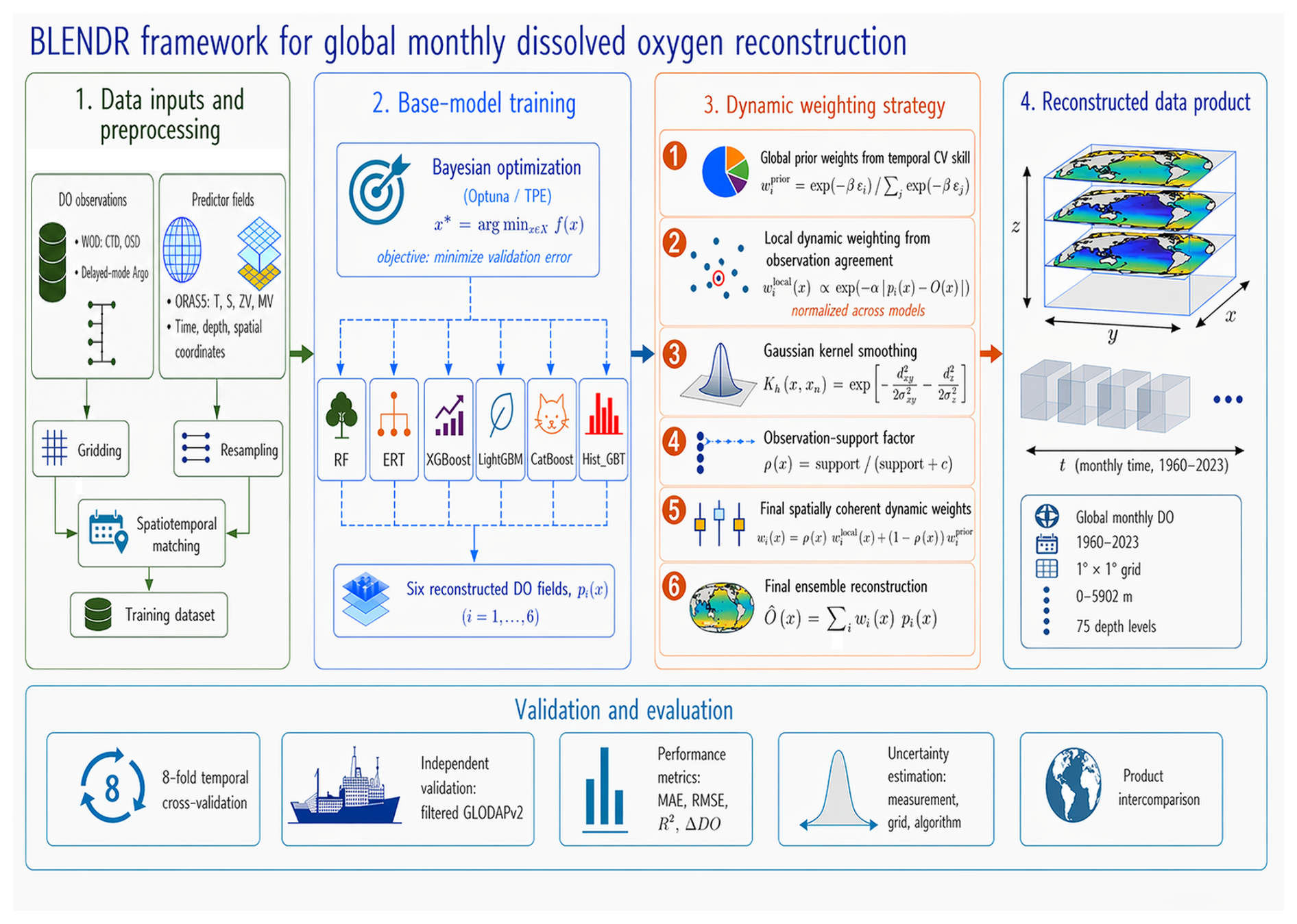
Figure 1 Overview of the BLENDR framework.

2.2.1 Data processing

In this study, all ocean DO observation data included temporal and spatial information, such as year, month, day, longitude, latitude, and measurement depth. The longitude and month are both periodic features. For instance, longitude ranges from 0 to 360°, with 360° overlapping with 0°, and month represents an annual cycle that repeats every 12 months. To address this issue, we followed the approach of Gade (2010) and Tang et al. (2019) by representing longitude and month using sine and cosine functions.

Although ORAS5 is provided on a 0.25° × 0.25° grid, we upscaled it by simple averaging to a common 1° × 1° grid with 75 depth levels. For each 1° grid cell, we averaged all available ORAS5 values located within that cell. DO observations were binned to each grid cell by averaging all points that fell within the cell at the same month and depth level. To address potential multicollinearity, which can lead to instability in subsequent modeling and increase the risk of overfitting, we analyzed correlations between the 11 factors. No correlation coefficient exceeded 0.5, so variable selection was not necessary in this case (Fig. S3). A complete list of predictors, with abbreviations and data sources, is shown in Table 1.

Table 1 Predictors, abbreviations and products/references of the 11 environmental factors.

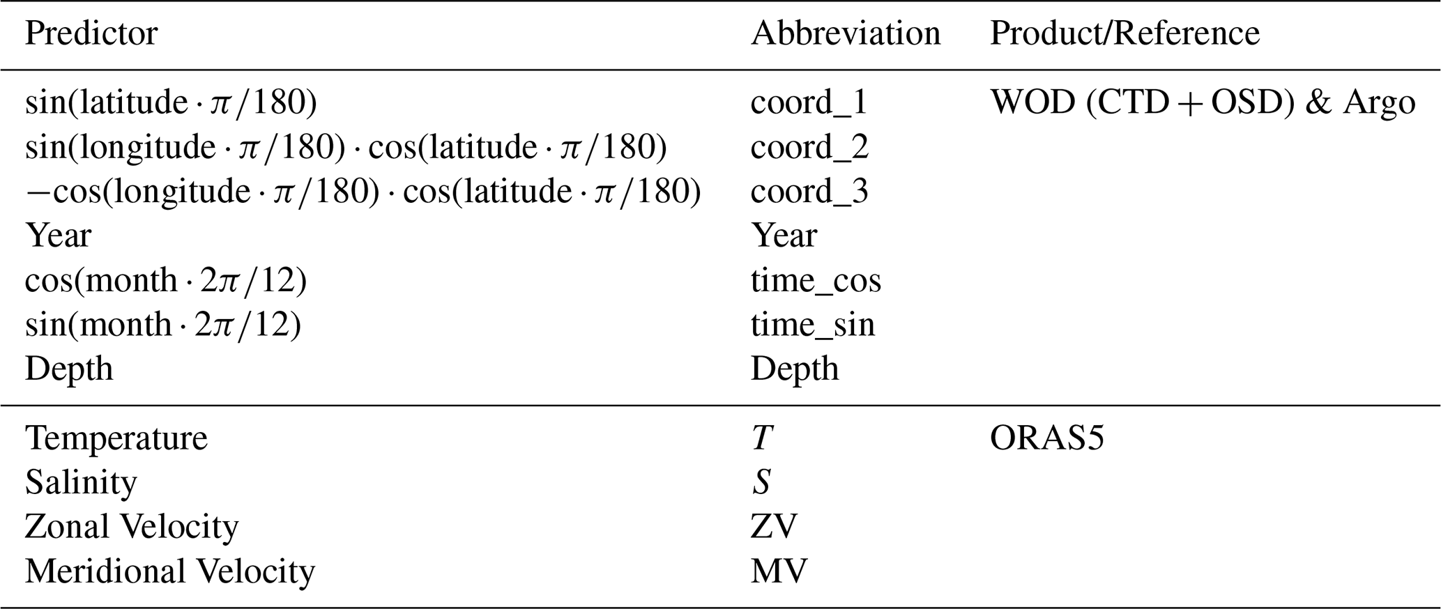
Note: The observational data were from WOD and Argo. The data from ORAS5 were 0.25° × 0.25° monthly mean profile data.

2.2.2 Machine learning models

We used six tree-based algorithms to reconstruct dissolved oxygen. Each model offers a different balance of bias, variance, and computational efficiency. We chose them because of their robust performance in regression tasks and their ability to handle nonlinear relationships. We used six models because they span the main tree learning paradigms, namely, bagging and boosting; thus, their strengths are complementary, and their residual errors are expected to be only weakly correlated. We kept the ensemble within the tree family because dissolved oxygen depends on nonlinear interactions among multiple drivers, and the data contain missing values, conditions under which decision trees perform well without elaborate feature engineering. In our initial model screening under the same input features and validation framework, the tested neural-network models, including a convolutional neural network and a back-propagation neural network, did not show an accuracy advantage over Random Forest, while requiring more tuning effort and providing less interpretability. Therefore, we focused the final ensemble on tree-based learners. All models were trained on the same input features and tuned via Bayesian optimization (Sect. 2.2.3). Below, we briefly describe each model.

Random Forest (RF) builds many decision trees on bootstrap samples and averages their outputs (Breiman, 2001). It selects a random subset of features at each split. This randomness reduces overfitting. RF handles large datasets well and is robust to outliers. RF represents classical bagging, and Extremely Randomized Trees (ERTs) push this idea toward stronger randomness (Geurts et al., 2006). It selects split thresholds at random rather than searching for the best cut. It uses the full dataset rather than bootstrapping. This strong randomization further lowers variance at modest cost in terms of bias. CatBoost is a gradient-boosting library designed for categorical features (Prokhorenkova et al., 2018). It uses ordered target statistics to avoid target leakage. It grows symmetric trees and performs efficient leaf pruning. CatBoost often converges faster and requires less tuning of the learning rate. XGBoost implements gradient boosting with second-order optimization (Chen and Guestrin, 2016). It adds regularization to control the complexity of the tree. It uses approximate split finding to speed up training on large data. XGBoost balances accuracy and runtime efficiency. LightGBM uses histogram-based binning and leaf-wise tree growth (Ke et al., 2017). It buckets continuous features into bins, reducing the amount of memory. Trees grow by selecting splits that yield the greatest loss reduction. LightGBM is highly efficient for large feature sets and large datasets. Histogram-based Gradient Boosting (Hist_GBT) follows Friedman's original gradient boosting framework (Guryanov, 2019; Friedman, 2001). It fits a sequence of weak learners to the negative gradient of the loss. It also uses histogram binning for faster split evaluation. Hist_GBT offers good accuracy in high-dimensional settings. XGBoost, LightGBM and Hist_GBT are gradient boosting methods but differ in terms of split criteria and optimization details.

2.2.3 Bayesian parameter optimization

To optimize hyperparameters across different machine learning models in a systematic and efficient manner, we employed Bayesian optimization using the Optuna framework (Akiba et al., 2019). Unlike grid or random search, this approach builds a statistical model of how settings affect error and then tests promising regions more often, finding good configurations with fewer trials and providing a fair, comparable procedure across models. Specifically, at each trial, a candidate set of hyperparameters is sampled, the model is trained, and its validation error is recorded. Optuna then uses all the previously tested hyperparameter–error pairs to update the surrogate model and proposes the next set of hyperparameters where the error is expected to decrease.

Bayesian optimization was used to construct a probabilistic surrogate model of the objective function f(x), where x is a vector of hyperparameters. The optimization seeks to identify the optimal x^* that minimizes f:

$$\begin{array}{}\text{(1)}& x^{*}=\underset{x\in \mathit{\chi }}{\arg min}f\left(\mathit{x}\right)\end{array}$$

Here, χ denotes the hyperparameter space. In practice, we used the Tree-structured Parzen Estimator (TPE) sampler in Optuna to approximate the objective function. After each trial, the observed pairs (x,f(x)) are divided into a “good” set with low objective values and a “bad” set with high values, using a quantile threshold. The TPE then fits two probability density functions over the hyperparameters, one for the good set and one for the bad set, and proposes new candidates in regions where the ratio of these densities is large. This strategy is equivalent to selecting the next sampling point to maximize the Expected Improvement (EI):

$$\begin{array}{}\text{(2)}& \mathrm{EI}\left(X\right)={\int }_{-\mathrm{\infty }}^{y*}(y^{*}-y)\cdot p\left(y\mathrm{|}x\right)\mathrm{d}y\end{array}$$

where y^* is the current best objective value. The sampling focuses on regions with high EI. In plain terms, the EI favors trials that are expected to reduce the error relative to the current best, so the search is concentrated on the most promising parts of the space.

To reduce temporal overfitting and preserve model generalizability across decades, hyperparameter optimization was conducted using a subset of data from eight years (1960, 1968, 1976, 1984, 1992, 2000, 2008, 2016). These years were chosen to sample different climate and sampling regimes across the six-decade period, ensuring that the optimized models are robust to temporal shifts in data availability and underlying oceanic conditions. The objective function minimized the Mean Squared Error (MSE) on an independent validation set derived from eight other test years (1967, 1975, 1983, 1991, 1999, 2007, 2015, and 2023). We chose the MSE because it penalizes large errors more heavily, which is desirable when evaluating gridded oxygen where occasional large deviations can dominate downstream diagnostics. The objective function was defined as follows:

$$\begin{array}{}\text{(3)}& \mathrm{MSE}={\displaystyle \frac{\mathrm{1}}{n}}\sum _{i=\mathrm{1}}^n({\widehat{y}}_i-y_i{)}^{\mathrm{2}}\end{array}$$

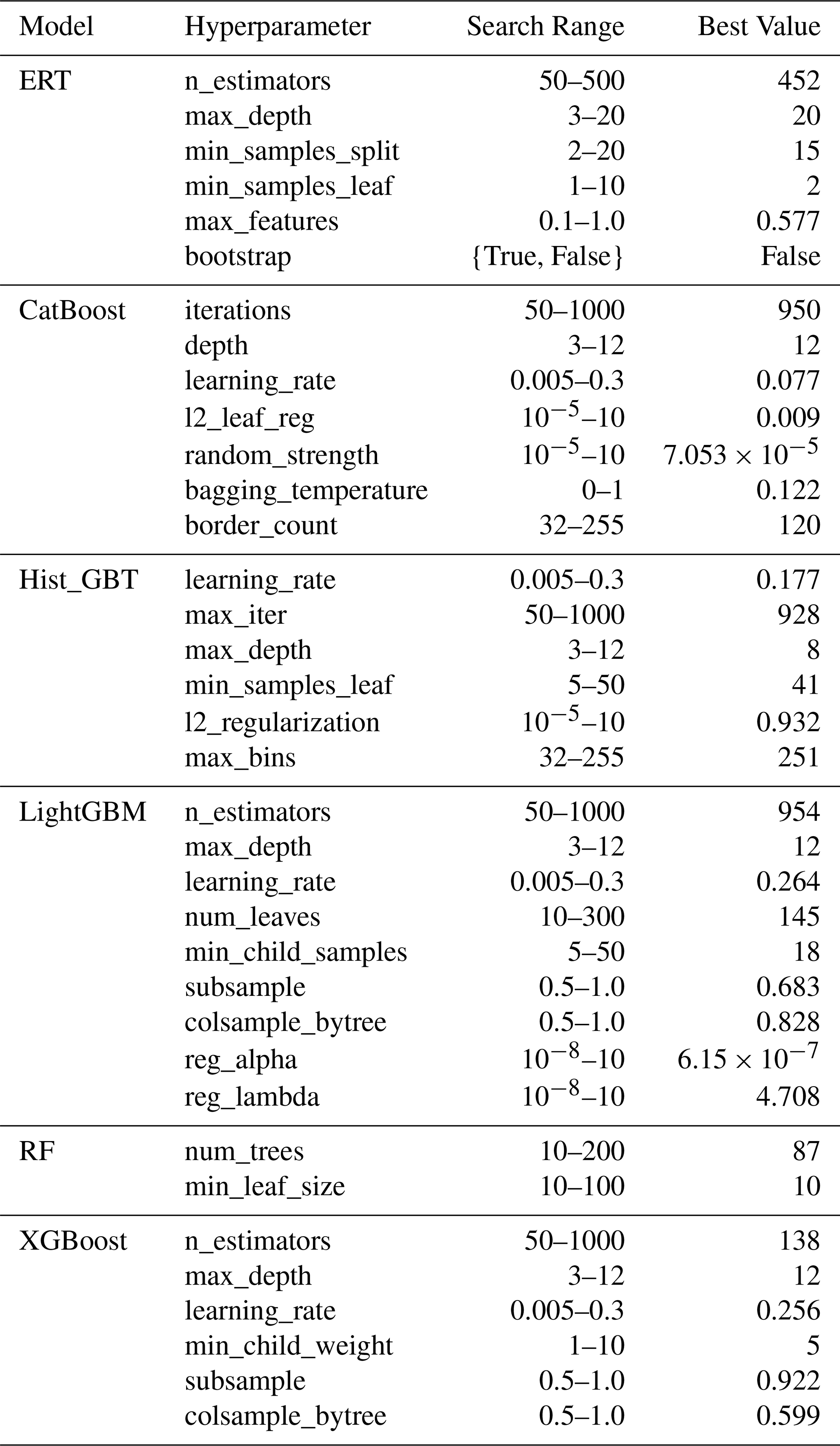
Each model was optimized over its own hyperparameter space, with the best-performing configuration recorded for final training and subsequent prediction on independent test data. This consistent, data-driven approach ensured fair comparability across all six learners and minimized bias from manual tuning. Below, we summarize the search space and optimal parameters in Table 2.

Table 2 Hyperparameter search spaces and optimal values.

2.2.4 Multi-model fusion and dynamic weighting scheme

We fused the predictions of the six base models into a single reconstruction using a spatially coherent dynamic weighting scheme. The aim was to combine global model skill with local observational constraint while maintaining spatial continuity in the weight field. This formulation is consistent with ensemble weighting based on model skill, locally calibrated weighting informed by nearby observations, and kernel-based estimation for spatially varying relationships (Raftery et al., 2005; Kleiber et al., 2011; Brunsdon et al., 1996). Each model was first assigned a global prior weight derived from its average predictive skill in temporal cross-validation. These prior weights served as a stable baseline in regions with weak observational support. We then introduced locally varying weights based on the agreement between model predictions and available observations. To avoid abrupt spatial changes in the weights, the local weights were further propagated to neighboring grid cells through Gaussian kernel smoothing and were gradually shrunk toward the global prior weights as observational support decreased.

We define the global prior weight ω_i of model i from its MAE ε_i in temporal cross-validation (Sect. 3.1) as

$$\begin{array}{}\text{(4)}& {\mathit{\omega }}_i={\displaystyle \frac{\exp (-\mathit{\beta }{\mathit{\epsilon }}_i)}{{\sum }_{j=\mathrm{1}}^M\exp (-\mathit{\beta }{\mathit{\epsilon }}_j)}}\end{array}$$

where M= 6 is the number of base models and β is the prior-weight sensitivity parameter. A smaller ε_i gives a larger ω_i, so models with better overall performance receive higher prior weights. Here, β controls how strongly the prior weights respond to differences in model MAE. We set β=1 to preserve the relative performance differences among models while avoiding excessively concentrated prior weights.

At grid cells with valid observations, we first define the local score of model i as

$$\begin{array}{}\text{(5)}& s_i\left(x\right)=\exp (-\mathit{\alpha }\mathrm{|}{p}_i(x)-O(x\left)\mathrm{|}\right)\end{array}$$

where p_i(x) is the prediction of model i at grid cell x, O(x) is the observed value. Here, α controls the sensitivity of local weighting to model error. We set α =1 to preserve the influence of local model-observation mismatch while avoiding excessively sensitive weight adjustments. These local scores are then normalized across all models to obtain the effective local weight at observation-supported grid cells:

$$\begin{array}{}\text{(6)}& l_i^{\mathrm{obs}}\left(x\right)={\displaystyle \frac{s_i\left(x\right)}{{\sum }_{j=\mathrm{1}}^M{s}_j\left(x\right)}}\end{array}$$

To extend the observational constraint smoothly to neighboring locations, we applied Gaussian kernel smoothing to the effective local weights. The kernel is defined as

$$\begin{array}{}\text{(7)}& K_{\mathrm{h}}(x,x_n)=\exp (-{\displaystyle \frac{d_{xy}(x,x_n{)}^{\mathrm{2}}}{\mathrm{2}{\mathit{\sigma }}_{xy}^{\mathrm{2}}}}-{\displaystyle \frac{d_z(x,x_n{)}^{\mathrm{2}}}{\mathrm{2}{\mathit{\sigma }}_z^{\mathrm{2}}}})\end{array}$$

where x_n denotes a neighboring grid cell, d_xy (x,x_n) is the horizontal distance between x and x_n, d_z (x,x_n) is the vertical distance, and σ_xy and σ_z control the smoothing scales in the horizontal and vertical directions, respectively. The smoothed local weight of model i is then written as

$$\begin{array}{}\text{(8)}& {\stackrel{\mathrm{̃}}{l}}_i\left(x\right)={\displaystyle \frac{{\sum }_{x_n\in N\left(x\right)}{K}_{\mathrm{h}}(x,x_n)l_i^{\mathrm{obs}}\left(x_n\right)}{{\sum }_{x_n\in N\left(x\right)}{K}_{\mathrm{h}}(x,x_n)}}\end{array}$$

where N(x) is the set of neighboring grid cells with valid effective local weights.

To quantify the degree of local observational support around each grid cell, we define

$$\begin{array}{}\text{(9)}& S\left(x\right)=\sum _{x_n\in N\left(x\right)}{K}_{\mathrm{h}}(x,x_n)\end{array}$$

and then construct an observation-support factor as

$$\begin{array}{}\text{(10)}& \mathit{\rho }\left(x\right)={\displaystyle \frac{S\left(x\right)}{S\left(x\right)+c}}\end{array}$$

where c is a shrinkage parameter. When observational support is strong, ρ(x) approaches 1 and the final weight is mainly controlled by the smoothed local weight. When observational support is weak, ρ(x) decreases and the final weight gradually returns toward the global prior weight.

Accordingly, the final weight of model i at grid cell x is defined as

$$\begin{array}{}\text{(11)}& w_i\left(x\right)=\mathit{\rho }\left(x\right){\stackrel{\mathrm{̃}}{l}}_i\left(x\right)+\left[\mathrm{1}-\mathit{\rho }\left(x\right)\right]{\mathit{\omega }}_i\end{array}$$

The final ensemble reconstruction is then calculated as

$$\begin{array}{}\text{(12)}& \widehat{O}\left(x\right)=\sum _{i=\mathrm{1}}^M{w}_i\left(x\right)p_i\left(x\right)\end{array}$$

2.2.5 Data reconstruction

We produced a global, monthly DO dataset on a regular 1° × 1° grid and 75 depth levels (0–5, 902 m) spanning from 1960 to 2023. First, we gathered all the predictor fields described in Table 1. Each field was remapped to the target grid and monthly time step consistent with ORAS5. Next, we applied the six optimized machine-learning models (Sect. 2.2.2) at every valid grid cell and time step. Each model ingested the full vector of predictors and returned a DO estimate only where all predictors were available. This yielded six parallel prediction arrays with dimensions 360 (longitude) × 180 (latitude) × 75 (depth) × 12 (months) × 64 (years from 1960 to 2023). We then merged these arrays using our spatially coherent dynamic weighting scheme (Sect. 2.2.4). Global prior weights reflected each model's cross-validation skill, whereas locally varying weights were derived from model agreement with available in situ observations. These local weights were then propagated to neighboring grid cells through Gaussian kernel smoothing and gradually shrunk toward the prior weights as observational support decreased. The weighted combination produces a single ensemble DO field for each grid cell and month. We packaged the ensemble field into a NetCDF file with coordinate variables, depth layers, time axes, and global attributes documenting the dataset and methods.

2.2.6 Argo oxygen data bias correction

Even after delayed-mode processing and standard quality control, Argo DO profiles are known to be systematically low relative to high-quality ship-based observations. To quantify the influence of a systematic offset in delayed-mode Argo, we produced two global reconstructions using the same machine-learning framework and predictors. The first was a standard reconstruction using CTD, OSD, and delayed-mode Argo profiles. The second was the bias-corrected reconstruction, which was otherwise identical but utilized the CTD, OSD, and delayed-mode Argo values adjusted by adding 1.69 µmol kg⁻¹ to every delayed-mode Argo measurement, following Wang et al. (2025). A comparison of the two reconstructions is shown in Sect. 5.5. All the other main results of the paper are based on the bias-corrected reconstruction.

3 Model performance

3.1 Model temporal cross-validation

We conducted 8-fold temporal cross-validation on each of the six models. In each fold f, data from eight test years $\mathit{\{}\mathrm{1960}+f+\mathrm{8}k{\mathit{\}}}_{k=\mathrm{0}}^{\mathrm{7}}$ formed the test set, with the remaining years for training. We trained each model using its optimized hyperparameters (Sect. 2.2.3) on the training set, predicted the DO values for the test years, and computed the mean bias (ΔDO), mean absolute error (MAE), root-mean-square error (RMSE), and coefficient of determination (R²) on the held-out data. These metrics collectively provide a comprehensive understanding of the model's predictive accuracy and bias. The results are presented in Tables S3–S6.

$$\begin{array}{}\text{(13)}& {\displaystyle }\mathrm{RMSE}=\sqrt{{\displaystyle \frac{\mathrm{1}}{\mathrm{n}}}\sum _{i=\mathrm{1}}^n(y_i-{\widehat{y}}_i{)}^{\mathrm{2}}}\text{(14)}& {\displaystyle }\mathrm{MAE}={\displaystyle \frac{\mathrm{1}}{\mathrm{n}}}\sum _{i=\mathrm{1}}^n\left|y_i-{\widehat{y}}_i\right|\text{(15)}& {\displaystyle }{R}^{\mathrm{2}}=\mathrm{1}-{\displaystyle \frac{\sum _{i=\mathrm{1}}^n(y_i-{\widehat{y}}_i{)}^{\mathrm{2}}}{\sum _{i=\mathrm{1}}^n(y_i-\stackrel{\mathrm{‾}}{y}{)}^{\mathrm{2}}}}\text{(16)}& {\displaystyle }\mathrm{\Delta }\mathrm{DO}={\displaystyle \frac{\mathrm{1}}{n}}\sum _{i=\mathrm{1}}^n(y_i-{\widehat{y}}_i)\end{array}$$

All six learners exhibited consistent skill across the eight temporal folds, with only minor spread in error metrics (Tables S3–S6). LightGBM displayed high stability, with MAEs varying by less than 1 µmol kg⁻¹ (10.11–11.04) and RMSEs under 1.3 µmol kg⁻¹ (16.38–17.59), yielding an R² range of 0.957–0.961. RF delivered the lowest RMSE (15.97–17.27) and highest R² (0.958–0.963). In contrast, CatBoost and Hist_GBT had slightly higher mean errors (MAEs of up to 11.04 and 11.42 and RMSEs of up to 17.57 and 17.99, respectively) and slightly greater inter-fold variability, indicating higher sensitivity to the specific training/test split (Tables S3–S6). Crucially, no model exhibited outlier folds with degraded performance, as all the models maintained MAEs < 12 µmol kg⁻¹ and R² > 0.95. This uniformity across folds confirms strong temporal generalization and validates our choice of an ensemble approach (Bergmeir and Benítez, 2012; Roberts et al., 2017).

3.2 Evaluation against independent observations

We evaluated both the ensemble and each individual model against an independent filtered GLODAPv2 dataset. Filtered GLODAPv2 profiles were averaged into the same 1° × 1° grid and monthly time step as the reconstructions.

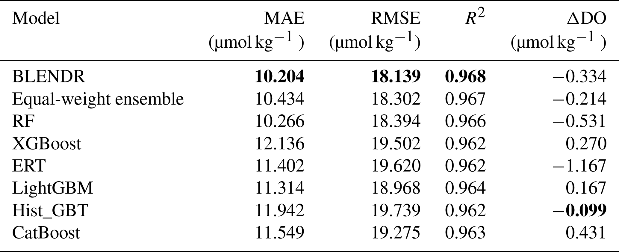
Table 3 demonstrates the clear advantage of the BLENDR framework. A stricter sensitivity test using a wider spatiotemporal exclusion criterion yielded very similar validation metrics (Table S7), suggesting that the main evaluation results are not sensitive to the original filtering choice. While the equal-weight ensemble outperformed most individual models, its MAE was still slightly higher than that of RF. This shows that simple averaging does not always outperform the best individual model, because weaker learners can still introduce additional errors. This improved performance is likely related to two reasons. BLENDR used each model's cross-validation skill and further optimized the weights through the spatially coherent dynamic weighting scheme. Among the individual algorithms, the RF and LightGBM performed best, whereas XGBoost and Hist_GBT performed at the lower end. All models had absolute biases below 1.2 µmol kg⁻¹. No individual method showed unstable or extremely poor performance in this evaluation, underscoring the robustness of our dynamic weighting in combining complementary strengths and minimizing weaknesses.

Table 3 Comparison of ensemble and individual models on the filtered GLODAPv2 dataset. Bold values indicate the best performance for each metric.

3.3 Uncertainty estimations

We quantified three distinct contributors to uncertainty in the reconstructed DO field, namely, measurement, grid, and algorithm uncertainty. These components were estimated separately and then combined to provide a first-order global uncertainty estimate.

The measurement uncertainty (O_meas) represents the random errors of the in situ dissolved oxygen observations. We adjusted the delayed-mode Argo DO values by adding a constant +1.69 µmol kg⁻¹ (Sect. 2.1.1), following the global bias assessment of Wang et al. (2025). After this bias correction, we treated Argo and CTD/OSD as unbiased on average, and O_meas represents only the residual random measurement error. We assumed constant uncertainties of 1 µmol kg⁻¹ for OSD and CTD and 3 µmol kg⁻¹ for Argo, following Ito et al. (2024). We then summarized a representative value across all observations using the root-mean-square of these assigned uncertainties.

The grid uncertainty (O_grid) quantifies the error associated with assigning a single value to a 1° × 1° grid cell. We estimated O_grid from the dispersion of collocated observations within each grid cell. For each grid cell with at least 10 collocated observations, we computed the within-cell standard deviation as follows:

$$\begin{array}{}\text{(17)}& \mathrm{\Delta }{O}_{\mathrm{grid}}=\mathit{\sigma }=\sqrt{{\displaystyle \frac{\mathrm{1}}{n-\mathrm{1}}}\sum _{i=\mathrm{1}}^n(O_i-\stackrel{\mathrm{‾}}{O}{)}^{\mathrm{2}}}\end{array}$$

where O_i is the ith observation in the cell and $\stackrel{\mathrm{‾}}{O}$ is the mean value of the observations. We then averaged σ over all qualifying cells to obtain a single global estimate of O_grid.

The algorithm uncertainty (O_alg) reflects the error introduced by the machine learning reconstruction process. We trained six models (RF, XGBoost, LightGBM, CatBoost, ERT, and Hist_GBT) using DO observations and environmental factors. Each model was optimized via Bayesian hyperparameter tuning and validated using an 8-fold cross-validation procedure, yielding an MAE for each model, denoted by error1 through error6. We then computed the prior weight for the ith model using an exponential decay function:

$$\begin{array}{}\text{(18)}& {\mathit{\omega }}_i={\displaystyle \frac{\exp (-{\mathrm{error}}_i)}{{\sum }_{j=\mathrm{1}}^{\mathrm{6}}\exp (-{\mathrm{error}}_j)}}\end{array}$$

and estimated the algorithm uncertainty as the weighted average of the MAE:

$$\begin{array}{}\text{(19)}& \mathrm{\Delta }{O}_{\mathrm{alg}}=\sum _{i=\mathrm{1}}^{\mathrm{6}}{\mathit{\omega }}_i{\mathrm{error}}_i\end{array}$$

Finally, the total uncertainty (O_total) in the reconstructed dissolved oxygen field is expressed as follows:

$$\begin{array}{}\text{(20)}& \mathrm{\Delta }{O}_{\mathrm{total}}=\sqrt{\mathrm{\Delta }{O}_{\mathrm{meas}}^{\mathrm{2}}+\mathrm{\Delta }{O}_{\mathrm{grid}}^{\mathrm{2}}+{\mathrm{\Delta }}_{a\lg }^{\mathrm{2}}}\end{array}$$

Using this framework, the estimated global component uncertainties were O_meas = 1.60, O_grid = 4.56, and O_alg = 10.29 µmol kg⁻¹, resulting in a combined global uncertainty of O_total= 11.37 µmol kg⁻¹.

4 Intercomparison with existing oxygen products

4.1 Comparison with filtered GLODAPv2 observations

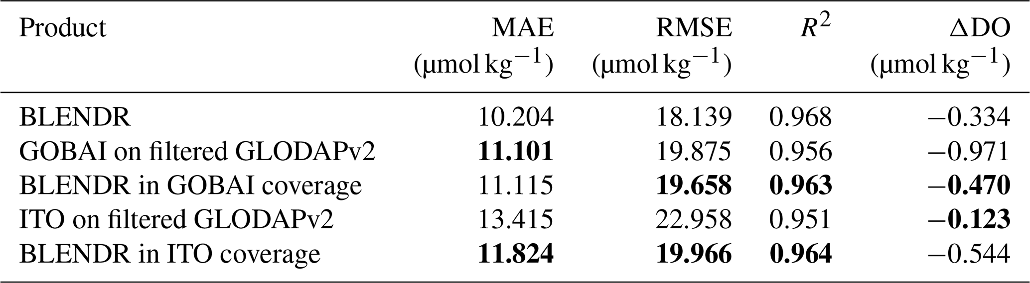
Compared with GOBAI (Sharp et al., 2023) and ITO (Ito et al., 2024), BLENDR showed the best overall agreement with the filtered GLODAPv2 reference dataset (Table 4). The comparison was conducted both over the full filtered GLODAPv2 dataset and within the coverage domains of GOBAI and ITO (Table 4). BLENDR achieved the lowest MAE and RMSE and the highest R² among the three products, with values of 10.204, 18.139 µmol kg⁻¹, and 0.968, respectively. Within the GOBAI coverage, BLENDR had a lower RMSE and a higher R² than GOBAI, although its MAE was slightly higher. Its mean bias was also closer to zero. Within the ITO coverage, BLENDR again showed lower MAE and RMSE and a higher R² than ITO, although its mean bias was farther from zero. Overall, these comparisons show that BLENDR compares favorably with existing products both over the full filtered GLODAPv2 comparison set and within their respective coverage domains.

Table 4 Performance comparison of BLENDR, GOBAI, and ITO against filtered GLODAPv2. Bold values indicate the best performance within each paired comparison domain. The GOBAI comparison is evaluated between “GOBAI on filtered GLODAPv2” and “BLENDR in GOBAI coverage”, while the ITO comparison is evaluated between “ITO on filtered GLODAPv2” and “BLENDR in ITO coverage”.

4.2 Comparison of mean vertical profile

The global mean vertical profile of BLENDR is broadly consistent with those of ITO Oxygen, WOA23, and the DIVA-based product of Roach and Bindoff (RB) over most of the water column (Fig. 2). The four profiles are very close near the surface. In the upper 0–1000 m, BLENDR, ITO, WOA23, and RB remain highly consistent. From about 1000 to 3500 m, the profiles of BLENDR, WOA23, and RB are nearly indistinguishable, indicating that BLENDR reproduces the large-scale deep-ocean oxygen structure well in this depth range. Below 3500 m, the profile of RB remains slightly closer to WOA23, but the differences among the products are still small. Overall, the mean-profile comparison shows that BLENDR remains close to the other products over most of the water column and reproduces the large-scale vertical structure consistently.

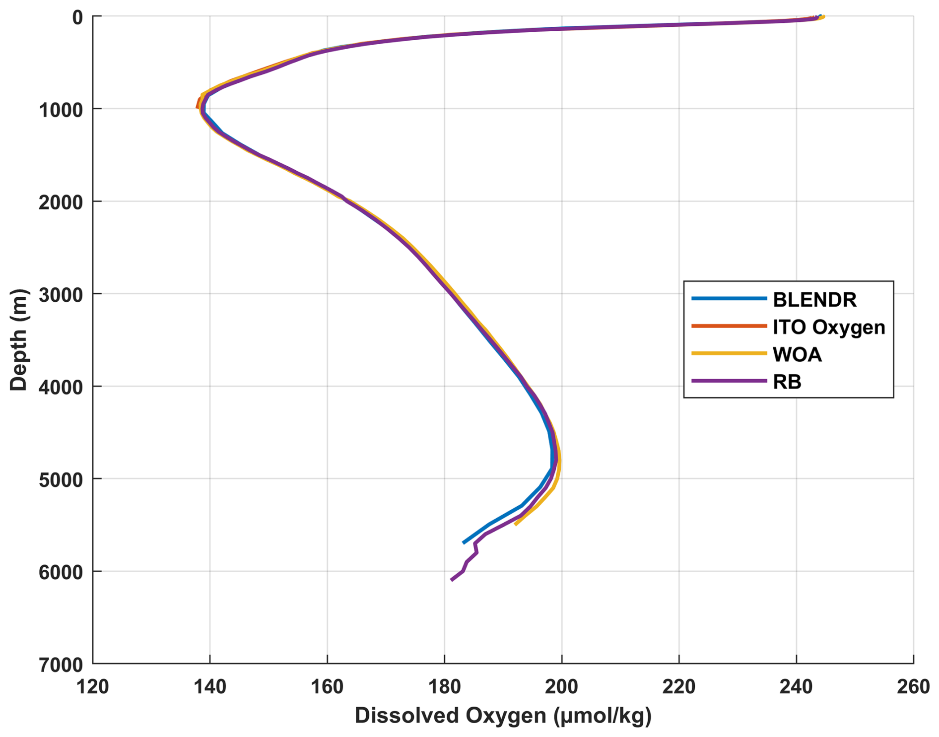
Figure 2 Global mean vertical profiles of different dissolved oxygen products (1965–2022). Solid lines show BLENDR (blue), Roach & Bindoff's reconstruction (purple), ITO Oxygen (orange) and WOA23 climatology (yellow), plotted from the surface down to 6000 m.

4.3 Spatial difference from climatological distribution

Relative to WOA23, BLENDR shows smaller large-scale departures than ITO in the upper layer and broadly comparable differences to RB in the deep layer (Figs. 3 and 4). Compared with ITO (Fig. 3), BLENDR is closer to WOA23, particularly in the surface layer, and shows smaller differences in many low- and mid-latitude regions. At around 10 m depth, BLENDR shows small differences, generally within ±2 µmol kg⁻¹, except in some high-latitude regions. In comparison, ITO exhibits broader regions where it is lower than WOA23 in the subtropical gyres and more pronounced regions where it is higher than WOA23 under the Antarctic Circumpolar Current. At around 30 m, the differences in BLENDR remain small in most mid-latitude regions, with larger variability near boundary currents. In contrast, ITO again shows larger departures in the subtropics and southern high latitudes. These results indicate that BLENDR is generally closer to WOA23 in the surface ocean. At around 200 m, both BLENDR and ITO Oxygen show larger departures from WOA23, reaching about ±10 µmol kg⁻¹ in the tropical and subtropical regions. At around 700 m, BLENDR and WOA23 remain within about ±8 µmol kg⁻¹ over large parts of the Atlantic and Pacific basins.

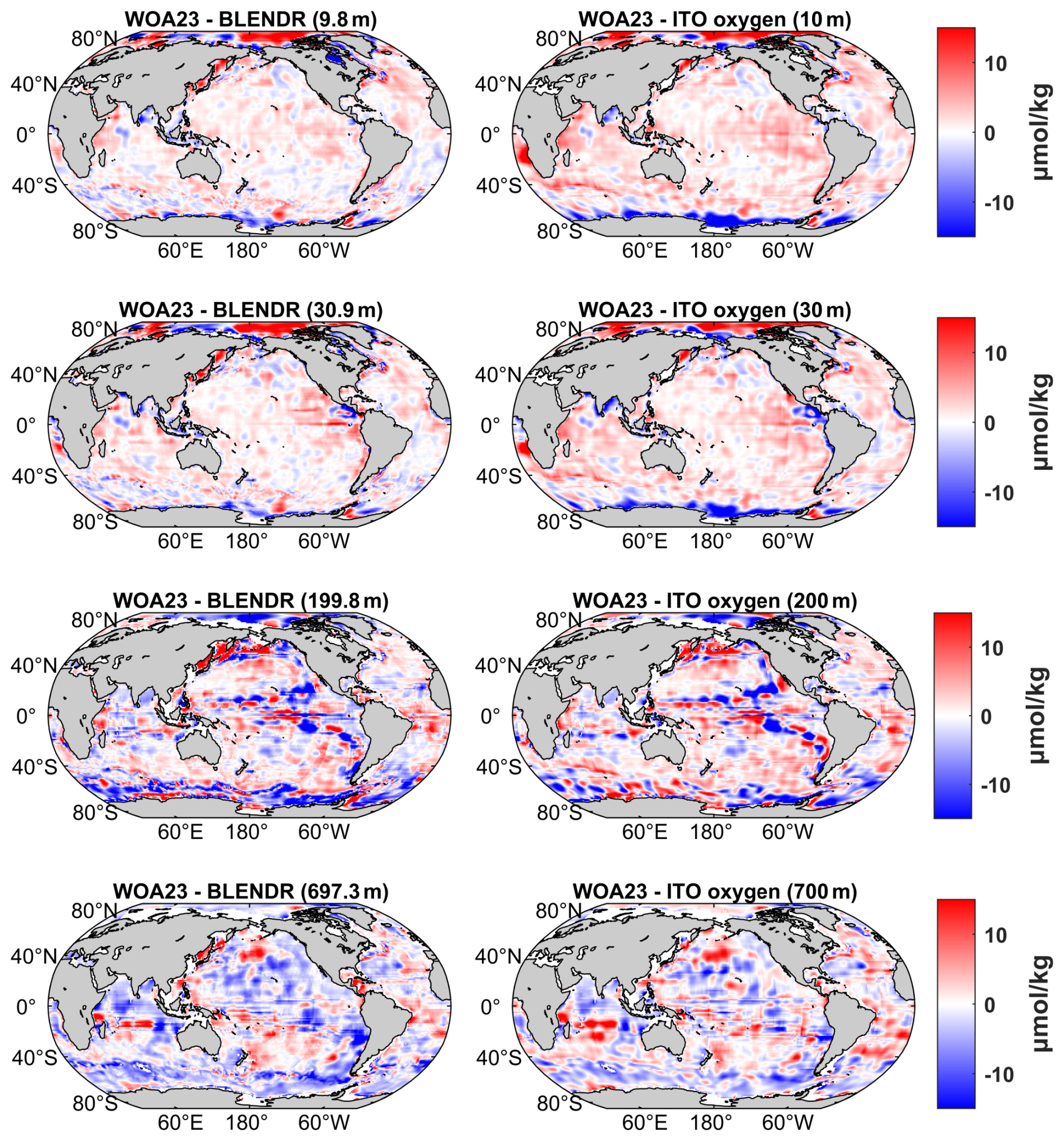
Figure 3 Spatial differences from WOA23 at four representative depths for BLENDR and ITO Oxygen. Left panels show WOA23 minus BLENDR at 9.8, 30.9, 199.8, and 697.3 m. Right panels show WOA23 minus ITO Oxygen at 10, 30, 200, and 700 m. Units are µmol kg⁻¹.

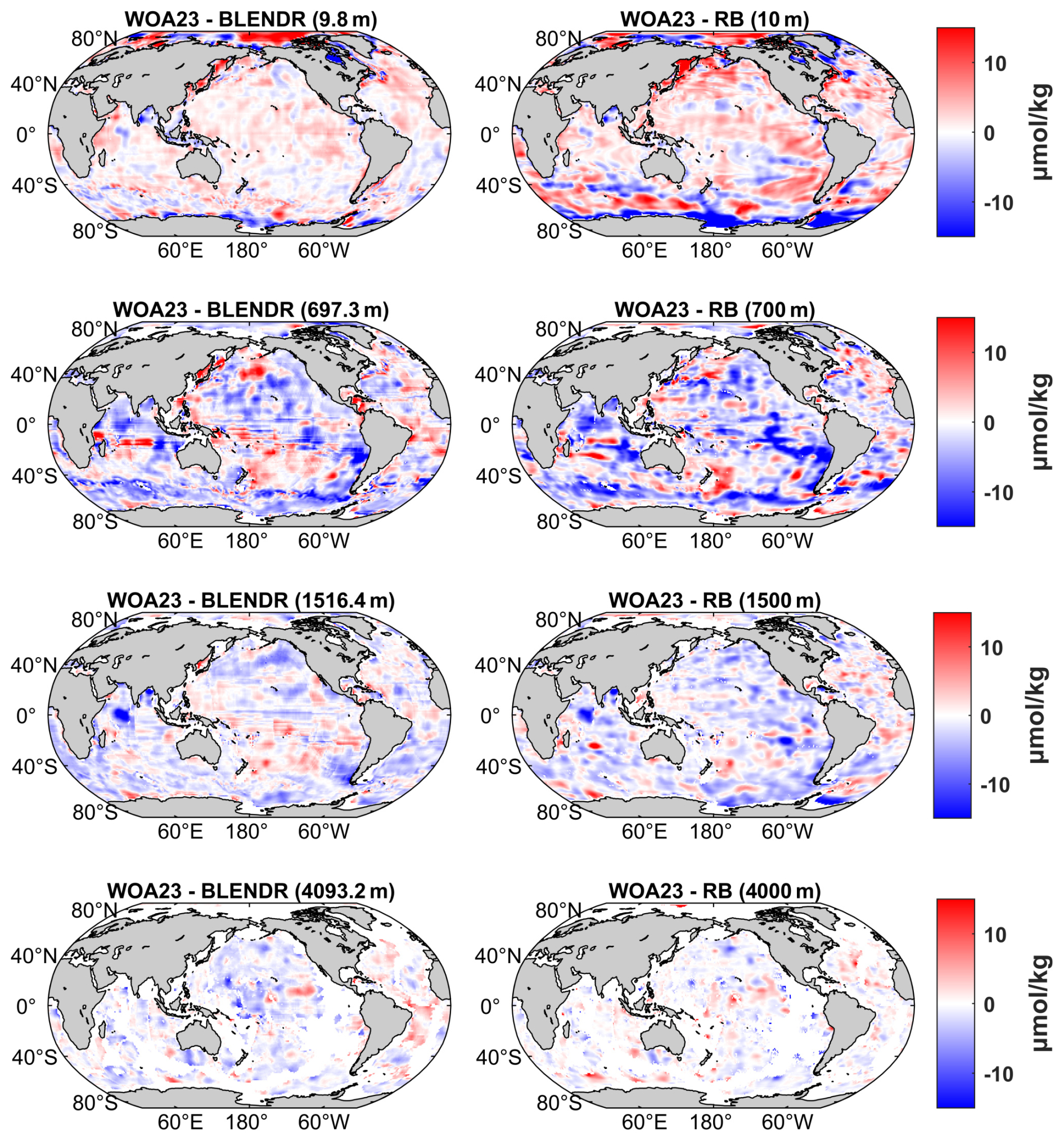
Figure 4 Spatial differences from WOA23 at four representative depths for BLENDR and the Roach and Bindoff (RB) product. Left panels show WOA23 minus BLENDR at 9.8, 697.3, 1516.4, and 4093.2 m. Right panels show WOA23 minus RB at 10, 700, 1500, and 4000 m. Units are µmol kg⁻¹.

In the comparison with RB, BLENDR shows a similar reduction in differences from WOA23 with increasing depth (Fig. 4). At around 10 m, BLENDR is generally closer to WOA23 than RB, with smaller spatial differences over much of the open ocean. At around 700 m, both BLENDR and RB show relatively large differences from WOA23. At around 1500 m, the differences decrease in both products, and at around 4000 m they decrease further, with both products showing generally smaller differences relative to WOA23. This comparison indicates that BLENDR agrees more closely with WOA23 in the surface layer, while in the deep ocean both BLENDR and RB show reduced differences below about 1500 m.

4.4 Comparison of oxygen content anomaly

BLENDR and ITO Oxygen show a similar multidecadal evolution of upper-ocean oxygen content anomaly during 1965–2020 (Fig. 5), with positive anomalies before the early 1990s, a rapid decline during the 1990s, and persistent negative anomalies after 2000. ITO Oxygen exhibits slightly larger anomaly amplitudes than BLENDR in the earlier part of the record, but the long-term downward trend and the timing of the transition from positive to negative anomalies are similar in both products. This result indicates that BLENDR is consistent with ITO Oxygen in capturing the large-scale decline of upper-ocean oxygen content.

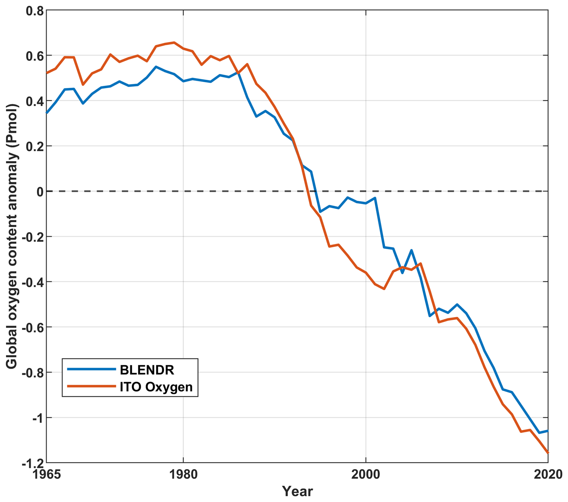
Figure 5 Global oxygen content anomaly in the upper 1000 m from BLENDR and ITO Oxygen during 1965–2020. The blue line denotes BLENDR and the orange line denotes ITO Oxygen. Anomalies are expressed in Pmol relative to the mean over the comparison period.

5 Global ocean DO distribution and trends

5.1 Spatial distributions along the vertical direction

Our reconstruction shows the full vertical extent of historical deoxygenation from the surface ocean to the abyss, providing continuous monthly fields down to 5902 m (Fig. 6a). The surface layer (0.5 m) is generally characterized by high DO concentrations, reflecting air–sea exchange and photosynthetic production (Ryther, 1956; Kolber et al., 2000). The especially high values at high latitudes (> 300 µmol kg⁻¹) are consistent with enhanced oxygen solubility in colder waters. At approximately 200 m, strong horizontal contrasts emerge, with broad low-oxygen regions in the eastern tropical Pacific and northern Indian Ocean (< 160 µmol kg⁻¹), while subpolar regions remain relatively oxygenated (> 200 µmol kg⁻¹). This rapid decrease reflects diminished gas exchange and ongoing microbial respiration (Keeling et al., 2010; Schmidtko et al., 2017). At approximately 850 m, the lowest DO concentrations are most evident, with the concentrations in the eastern Pacific and northern Indian Ocean decreasing below 150 µmol kg⁻¹, whereas the North Atlantic (NA) mid-depth ocean maintains higher concentrations (180–200 µmol kg⁻¹). In the bathypelagic zone (∼ 4000 m), DO becomes spatially uniform (180–200 µmol kg⁻¹) across basins, which is consistent with the large-scale deep-water mass structure (Talley, 2013). Overall, along the water column, the DO concentration peaks at the surface and reaches a local minimum of approximately 139 µmol kg⁻¹ near the classical OMZ at approximately 1000 m but then slowly increases toward 200 µmol kg⁻¹ at approximately 4500 m (Fig. 6b).

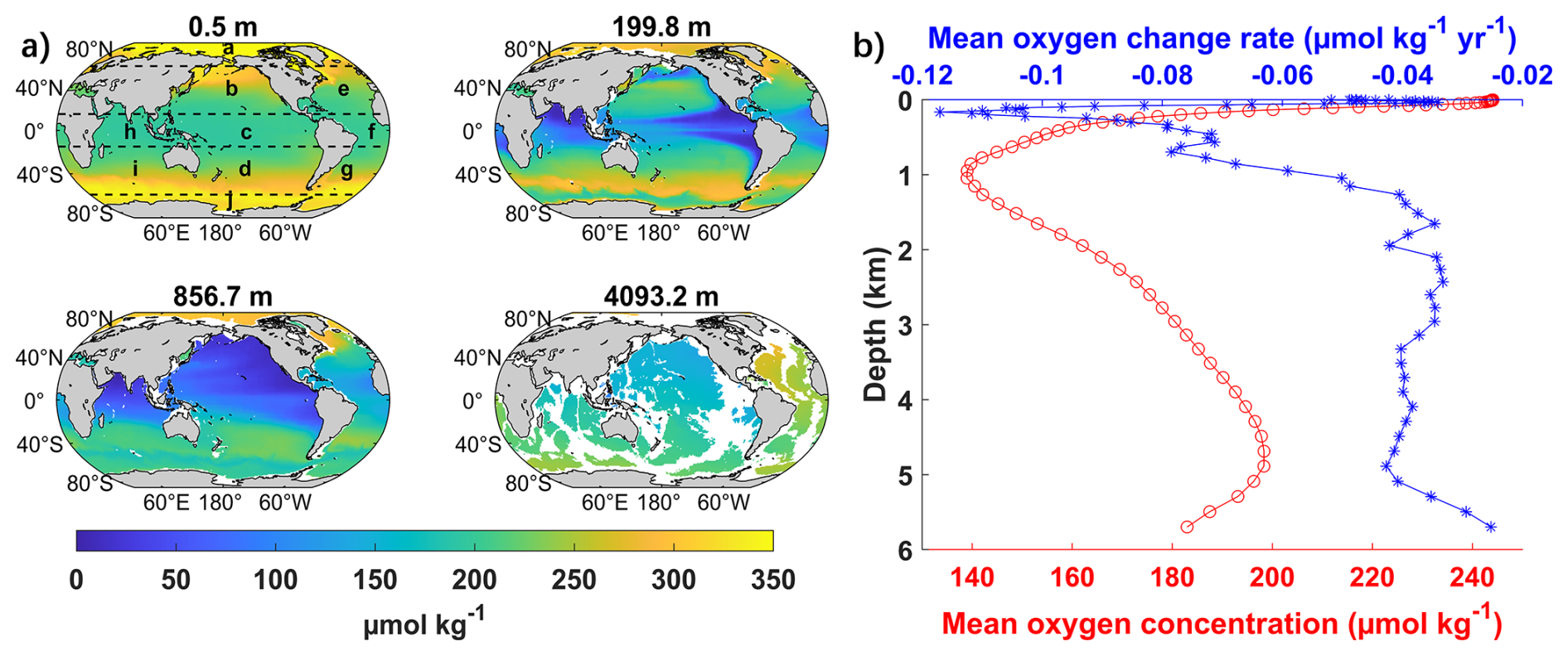
Figure 6 Global distribution and vertical structure of dissolved oxygen. (a) Climatological mean dissolved oxygen concentration at four representative depths (0.5, 199.8, 856.7, and 4093.2 m) from the reconstructed global product. Letters indicate the ten regions: (a) Arctic Ocean (AO), (b) North Pacific (NP), (c) Equatorial Pacific (EP), (d) South Pacific (SP), (e) North Atlantic (NA), (f) Equatorial Atlantic (EA), (g) South Atlantic (SA), (h) Equatorial Indian (EI), (i) South Indian (SI), and (j) Southern Ocean (SO). This regionalization scheme is adopted from Schmidtko et al. (2017). (b) Global mean vertical profiles of the dissolved oxygen concentration (red; µmol kg⁻¹) and its long-term linear change rate (blue; µmol kg⁻¹ yr⁻¹).

The global mean DO trend from 1960 to 2023 was negative at nearly all depths, with the strongest deoxygenation in the subsurface ocean and weaker trends in the surface and deep ocean (Fig. 6b). While the deoxygenation rate was low (−0.04 µmol kg⁻¹ yr⁻¹) at the surface, the decline accelerated greatly below 60 m, reaching its most negative values between 150 and 200 m (−0.12 µmol kg⁻¹ yr⁻¹). This pattern reflects an amplification of shallow subsurface oxygen loss, most likely driven by stronger stratification that inhibits ventilation exchange and by increased microbial respiration (Keeling et al., 2010; Schmidtko et al., 2017).

5.2 Depth-basin patterns in the OMZ area

Over the past six decades, the OMZ (DO < 60 µmol kg⁻¹) has existed primarily at depths between 100 and 2000 m, but its vertical structure and magnitude vary strongly between basins (Fig. 7). In the global mean profile, the total OMZ area increases from the surface to a broad maximum near 800 m and then decreases toward deeper waters. In the North Pacific (NP), the OMZ is thickest, with a wide band of large area between approximately 800 and 1200 m, which is consistent with slow intermediate-water ventilation and long residence times that allow for respiration to consume oxygen (Karstensen et al., 2008; Paulmier and Ruiz-Pino, 2009). In the North Indian (NI), by contrast, the largest OMZ area is much shallower, between approximately 100 and 1000 m, reflecting a combination of weak thermocline ventilation and strong export production in the Arabian Sea and Bay of Bengal that produces very intense hypoxia (Naqvi et al., 2006; Keeling et al., 2010). The Equatorial Pacific (EP) and Equatorial Atlantic (EA) have thinner OMZ layers centered at approximately 300–600 m. The OMZ in the EP is located primarily in the eastern ocean because of relatively stagnant cyclonic gyres north and south of the equator in the east subsurface layers, which are poorly ventilated (Keeling et al., 2010). In the Atlantic, the OMZ area is much smaller than that in the Pacific, which is consistent with stronger ventilation of the Atlantic thermocline and intermediate waters (Stramma et al., 2008; Talley, 2013).

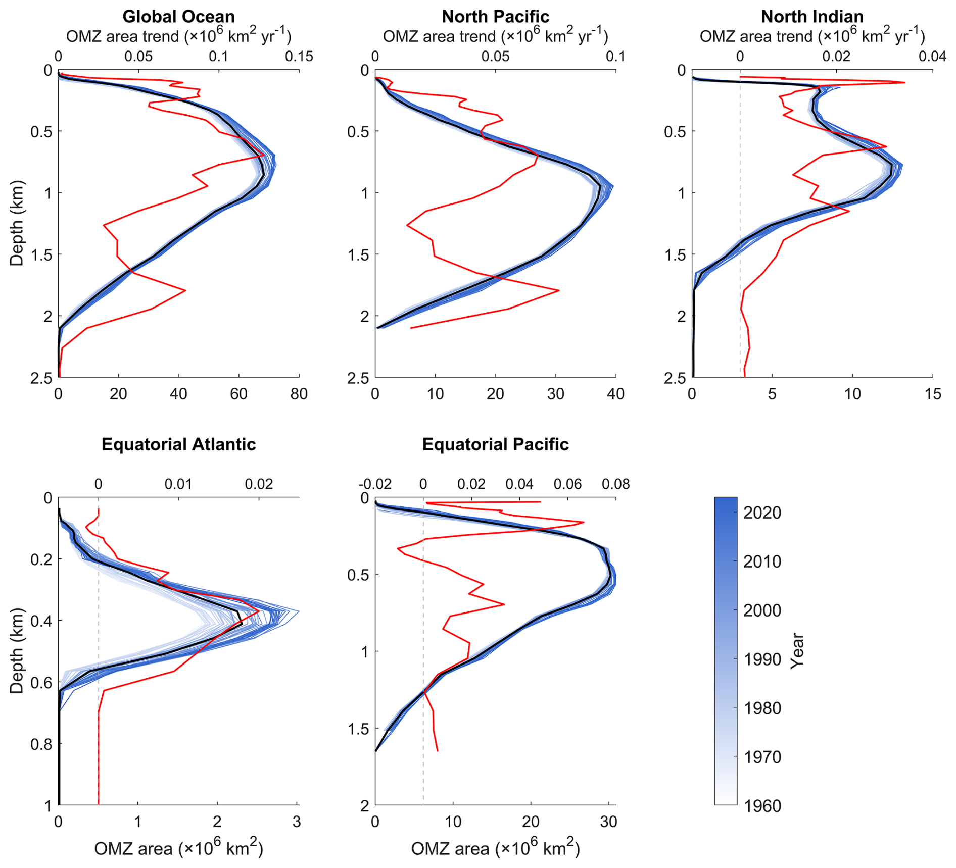
Figure 7 Vertical evolution of the OMZ area across major ocean basins during 1960–2023. Vertical profiles of the annual OMZ area (blue lines; threshold = 60 µmol kg⁻¹) for the global ocean and four major basins: North Pacific, North Indian, Equatorial Atlantic, and Equatorial Pacific. Individual blue curves represent yearly OMZ area profiles, with color shading indicating the year (1960–2023). The black curves show the long-term mean OMZ area at each depth. The red curves denote the linear trend in the OMZ area with depth (× 10⁶ km² yr⁻¹), highlighting the depth-dependent expansion or contraction of low-oxygen waters. Here, the North Indian includes the Equatorial Indian labeled h in Fig. 6a, together with the Bay of Bengal and Arabian Sea.

These basin differences are also reflected in the vertical profiles of the OMZ extent. OMZ extents have distinct depth profiles across the regions: the NP, EP, and EA are characterized by a single local maximum, whereas the North Indian Ocean (including the Arabian Sea and Bay of Bengal) exhibits two local maxima, suggesting periodic intrusions of oxygen-rich water (Jain et al., 2017; Sarma and Udaya Bhaskar, 2018). The high productivity in the western Arabian Sea region leads to increased oxygen consumption (Acharya and Panigrahi, 2016), whereas the oxygen-rich Somali Current, approximately 500 m deep, introduces oxygen, particularly during summer (Zhang et al., 2022), resulting in weaker OMZs at this depth. Persian Gulf Water (PGW) in the Bay of Bengal contributes to a modest increase in oxygen at 350–450 m (Jain et al., 2017), resulting in a reduced OMZ. These intrusions disrupt the continuity of OMZs, leading to the dual-minima pattern observed in these regions. This phenomenon highlights the complex and dynamic nature of OMZ distribution and its susceptibility to various oceanographic processes.

Over the 1960–2023 period, the OMZ area profile gradually expanded across nearly all depths in terms of the global mean and most basins (Fig. 7). These changes indicate a significant shift in the vertical distribution and extent of low-oxygen seawater globally over the past six decades. Specifically, the global OMZ extent growth rate was highest at 400–1000 m because of expansion across all regions, with its peak at 600–700 m due to expansion in the EP and NP. Therefore, while the largest OMZ extent was approximately 900 m, shifts to the much shallower 600–700 m layer are likely in the future. After this peak, the horizontal expansion rate of the OMZ decreased, with the lowest rates occurring at 1300–1600 m. However, the expansion rates increased again beyond 1600 m because of growth in the NP.

5.3 Basin-scale deoxygenation and spatial trend patterns

Deoxygenation was more negative after 2010 across all major ocean basins, indicating stronger recent oxygen loss over the 1960–2023 record (Fig. 8). During the period from 1960 to 2010, the deoxygenation rates were generally modest. The greatest loss (91.4 ± 17.7 Tmol per decade) occurred in the NP, followed by the Southern Ocean (SO) (86.8 ± 10.5 Tmol per decade) and South Atlantic (SA) (68.3 ± 10.4 Tmol per decade). In the Southern Indian (SI) and South Pacific (SP) basins, the deoxygenation trends from 1960 to 2010 were almost negligible. This likely reflects the much sparser observational coverage in the Southern Hemisphere during the early record than during the Argo era.

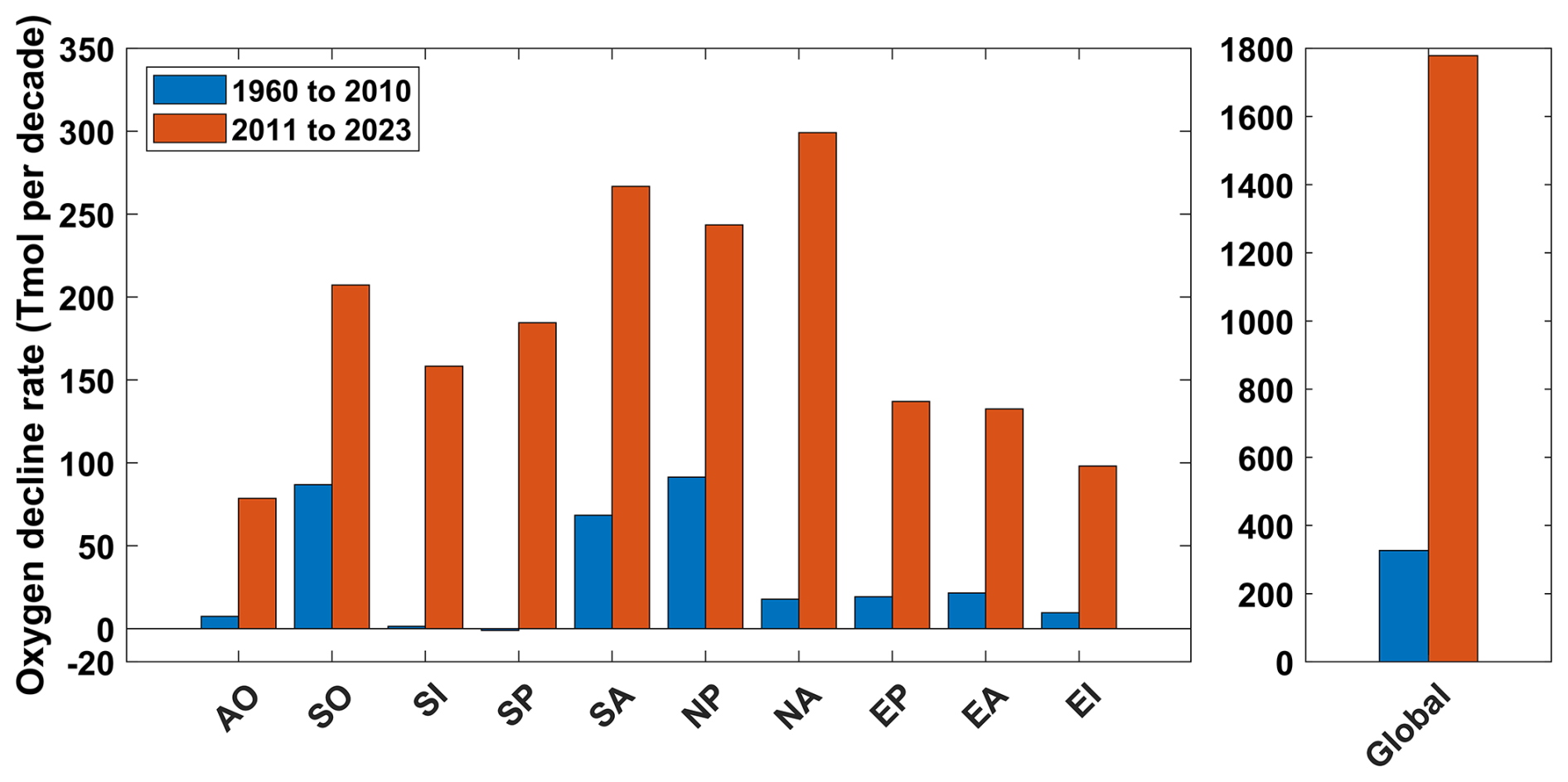
Figure 8 Decline in oxygen rates across major ocean basins. Decadal oxygen decline rates are shown for ten individual ocean basins and for the global ocean and were estimated separately for 1960–2010 (blue) and 2011–2023 (orange).

In the period after 2010, oxygen loss trends significantly increased across all the basins. The NA loss increased by more than a factor of 16 to 299.1 ± 45.8 Tmol per decade. The SA and NP both exceeded 240 Tmol per decade. The Arctic Ocean (AO) accelerated from near zero to 78.6 ±18.1 Tmol per decade. This recent acceleration of oxygen loss is attributed to amplified warming of Atlantic inflow from the 2000s to the 2010s, which reduces oxygen solubility and advects low-oxygen waters into the basin (Wu et al., 2025).

The spatial distribution of dissolved oxygen trends during 2011–2023 shows widespread deoxygenation in both the upper layer (0–1516 m) and the deep layer (1516–5902 m), with the upper layer exhibiting stronger magnitudes and greater spatial heterogeneity (Fig. 9). Compared with 1960–2010, the 2011–2023 period exhibits much stronger and more spatially heterogeneous linear trend patterns in both layers, whereas the earlier period is characterized by weaker and more spatially uniform changes.

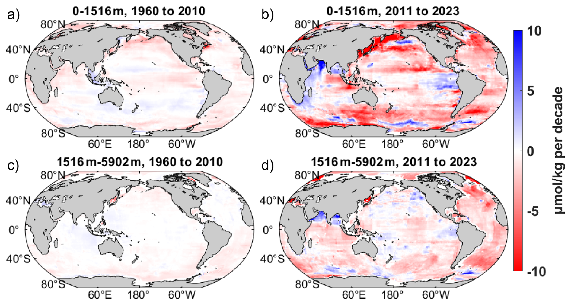
Figure 9 Spatial distribution of dissolved oxygen trends for the upper layer (0–1516 m) and deep layer (1516–5902 m) during 1960–2010 and 2011–2023. Panels (a) and (b) show the upper-layer trends for 1960–2010 and 2011–2023, respectively, and panels (c) and (d) show the corresponding deep-layer trends. Trends are expressed in µmol kg⁻¹ per decade. Positive values indicate oxygen increase, and negative values indicate oxygen decrease.

Although negative trends dominate much of the Pacific, Atlantic, and Southern oceans during 2011–2023, several spatially confined regions of positive trends are also evident. These include the eastern equatorial Pacific (Espinoza-Morriberón et al., 2019), the Southern Ocean (Iida et al., 2013; Morrison et al., 2022), and the North Indian Ocean (Narvekar et al., 2025; Nayak et al., 2025). Some of these localized increases may reflect interannual to decadal variability over the short 2011–2023 period rather than persistent long-term change. These spatial patterns are nevertheless broadly consistent with previous regional studies linking oxygen increases to variability in circulation, ventilation, mixing, and oxygen supply (Karstensen et al., 2008; Espinoza-Morriberón et al., 2019; Busecke et al., 2019; Duteil et al., 2021; Morrison et al., 2022; Narvekar et al., 2025; Nayak et al., 2025). Overall, deoxygenation remains the dominant large-scale signal during 2011–2023, while regional oxygen increases are confined to a few dynamically distinct areas.

5.4 Hemispheric seasonal variability in dissolved oxygen

Along the water column, the seasonal amplitude was strongest in the surface layer, which responds rapidly to the seasonal changes in air–sea gas exchange, surface heating and cooling, and biologically driven production and respiration. In contrast, the seasonal cycles in the thermocline and intermediate ocean (∼ 100–1500 m) were substantially weaker, with anomalies typically ±1 µmol kg⁻¹, and those in the deep ocean (> 1500 m) were nearly constant throughout the year, with amplitudes below 0.1 µmol kg⁻¹ (Fig. 10). This rapid vertical decline in seasonality is consistent with the dominant control mechanisms in the ocean interior. Away from the surface, oxygen is mainly controlled by the ventilation of intermediate waters and by the slow remineralization of sinking organic matter. These processes evolve on multiyear to decadal time scales; thus, these water masses respond weakly to the seasonal cycle (Keeling et al., 2010; Talley, 2013). At abyssal depths, water masses are ventilated in high-latitude formation regions and subsequently spread via slow interior circulation; thus, oxygen variability is controlled mainly by large-scale and long-term transport changes (Oschlies et al., 2018).

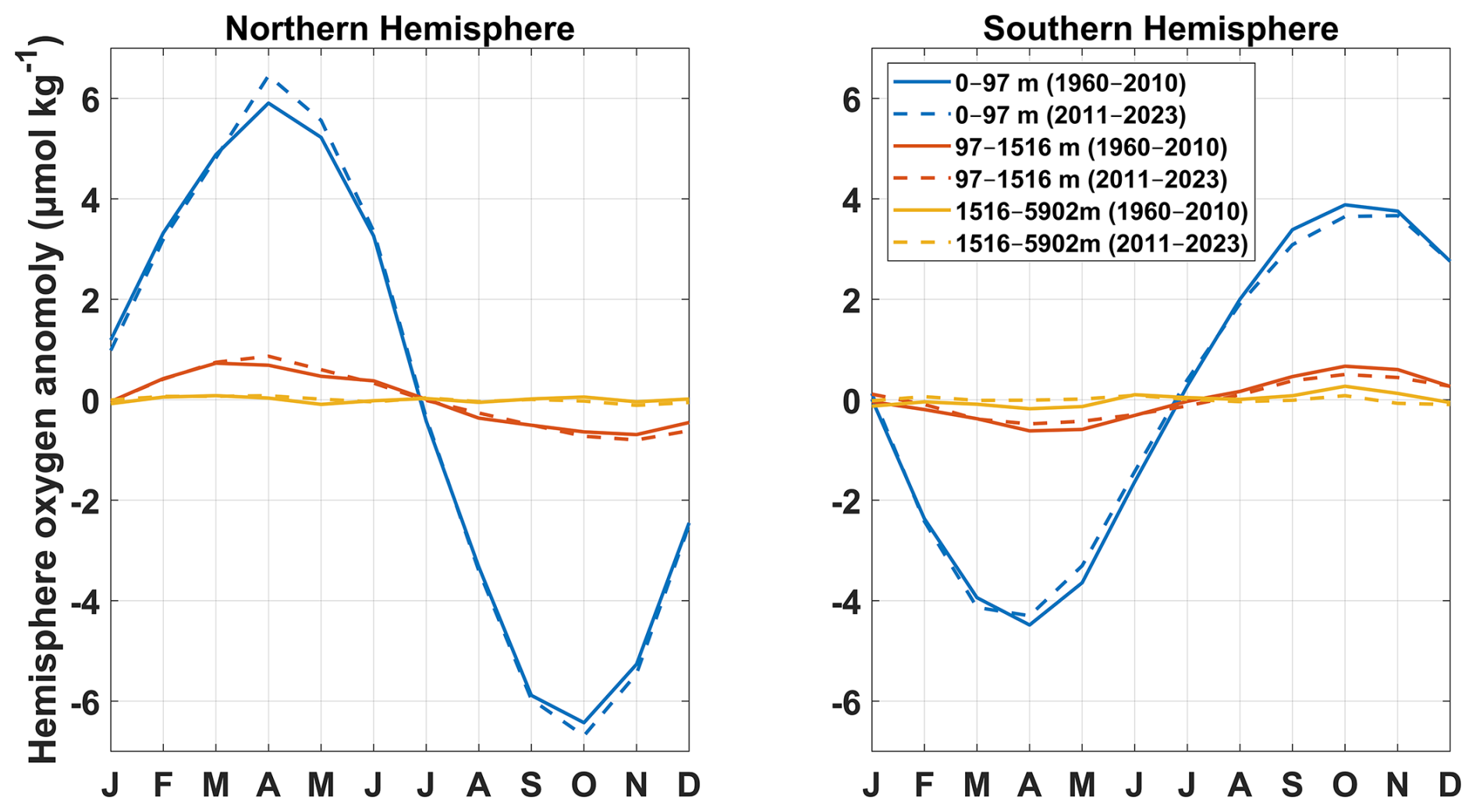
Figure 10 Climatological seasonal cycle of hemispheric mean dissolved-oxygen anomalies. The left panel shows the Northern Hemisphere and the right panel shows the Southern Hemisphere. The blue lines denote the surface layer (0–97 m), the red lines denote the thermocline and intermediate layer (97–1516 m), and the yellow lines denote the deep ocean (1516–5902 m). The solid lines represent anomalies from 1960 to 2010, and the dashed lines represent anomalies from 2011 to 2023.

Comparing 1960–2010 with 2011–2023, the NH surface DO amplitude intensified, whereas the SH weakened. This hemispheric contrast is consistent with the direct dependence of oxygen on temperature and with the positive correlation between changes in the seasonal amplitude of surface DO and SST (Fig. S4). In recent decades, the sea surface temperature (SST) seasonal amplitudes in large parts of the Northern Hemisphere have increased, whereas in the Southern Ocean, the SST seasonal cycle has shown robust weakening since the 1950s (Fig. S5). Upper-ocean temperature seasonal amplitudes generally increased in the AO and other northern basins but weakened in the Southern Ocean. This pattern is consistent with the opposing NH–SH changes in DO seasonality from our reconstruction.

The Northern Hemisphere (NH) displays a larger seasonal amplitude than the Southern Hemisphere (SH), with peak anomalies in the surface and mid-layer ocean approximately 50 % greater. A main contributor is the larger NH seasonal temperature range than the SH, which amplifies the seasonal cycle of oxygen solubility and therefore the seasonal cycle of oxygen saturation capacity (Fig. S5). Biological processes further enhance these differences. Satellite chlorophyll-a climatology indicates that the seasonal amplitude of phytoplankton biomass is generally larger at mid- and high northern latitudes than at corresponding southern latitudes (Mao et al., 2020), consistent with a stronger seasonal DO response in the NH. Phytoplankton blooms can drive transient surface DO supersaturation in spring, whereas warmer summer conditions can increase heterotrophic respiration (Frajka-Williams et al., 2009; Carstensen et al., 2014). Argo-based analyses show that, although both hemispheres exhibit enhanced upper-ocean stratification in their respective summer seasons, the NH typically shows stronger stratification maxima than the SH (Roch et al., 2023), which limits resupply and intensifies late-summer and early-fall DO minimum (Rippeth et al., 2024).

5.5 Effect of Argo bias correction on the reconstructed oxygen estimates

The global time series from 1960 to 2023 confirms a long-term and large-scale decline in total dissolved oxygen content (Fig. 11a). Over the full analysis period, both our standard and bias-corrected reconstruction methods indicate a persistent decline, with total losses of 5.4 ± 0.5 and 4.1 ± 0.4 Pmol, respectively. This corresponds to overall decreases of 2.3 ± 0.2 % and 1.8 ± 0.2 %, respectively. This magnitude of loss is consistent with prior synthesis estimates of historical deoxygenation, such as approximately 4.8 ± 2.1 Pmol of oxygen loss since 1960 by Schmidtko et al. (2017) and an overall ∼ 2 % decrease in oxygen in the late 20th century by Helm et al. (2011).

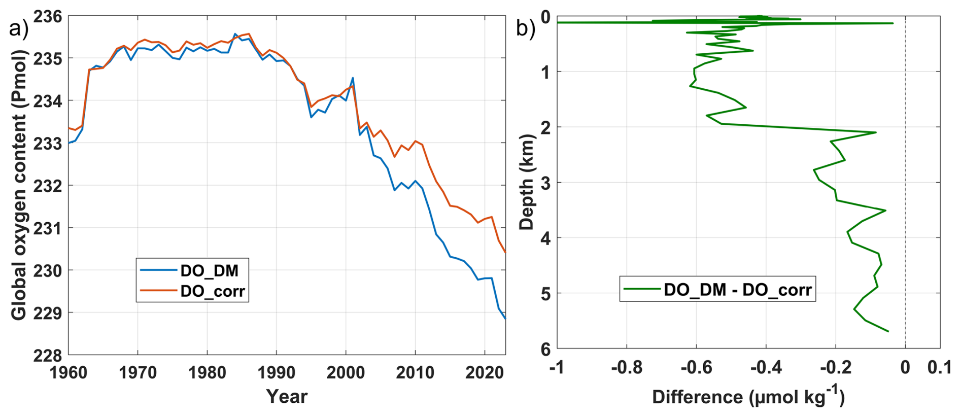
Figure 11 Comparison of global ocean oxygen content and annual mean climatology with and without Argo DO bias correction. (a) Time series of globally integrated ocean oxygen content from 1960 to 2023 based on two reconstructions that use the same machine-learning framework applied to observational oxygen profiles. The blue curve (DO_DM) used oxygen measurements from the CTD, OSD, and delayed-mode Argo profiles. The red curve (DO_corr) used the same inputs but applied a +1.69 µmol kg⁻¹ bias correction to all the Argo DO profiles following Wang et al. (2025). (b) Annual mean vertical profile of the difference between the two reconstructions (DO_DM – DO_corr).

The Argo bias correction produces only modest changes in the reconstructed oxygen fields and does not substantially affect the long-term deoxygenation rates (Fig. 11a). Both the standard and the bias-corrected reconstructions strongly agree prior to 2005, when the observations are constrained mainly by ship-based CTD and OSD measurements. After 2005, when the Argo observations became a significant contributor, the reconstruction that incorporates bias-corrected Argo data yielded a slightly higher global mean oxygen content than the uncorrected version did. Consequently, the bias-corrected reconstruction showed a greater global oxygen content in recent years. Vertically, the greatest differences occurred above 2000 m, where the difference mostly ranged from −0.4 to −0.6 µmol kg⁻¹ (Fig. 11b), due to dense Argo float sampling and strong optode biases at this depth. Beyond 2000 m, where sampling mainly comprised sparse ship-based measurements, the difference decreased to −0.2 µmol kg⁻¹, and below approximately 3500 m, the two reconstructions were almost indistinguishable. In summary, the Argo bias correction improves cross-platform consistency but has only a limited influence on global and basin-scale conclusions drawn from the reconstruction.

6 Data availability

The reconstructed global monthly dissolved oxygen dataset produced in this study is publicly available in NetCDF format via Zenodo at https://doi.org/10.5281/zenodo.19705526 (Han and Zhou, 2026) under a Creative Commons Attribution 4.0 license. Source DO profile observations were obtained from the International Argo Program and the national programs that contribute to Argo (https://argo.ucsd.edu, last access: 5 March 2025), the World Ocean Database 2023 (WOD) maintained by the U.S. National Oceanic and Atmospheric Administration (NOAA; https://www.ncei.noaa.gov/products/world-ocean-database, last access: 5 March 2025), and the Global Ocean Data Analysis Project v2.2023 (GLODAPv2; https://www.ncei.noaa.gov/access/ocean-carbon-acidification-data-system/oceans/GLODAPv2_2023, last access: 5 March 2025). Environmental predictor fields were drawn from the ORAS5 ocean reanalysis provided by the European Centre for Medium-Range Weather Forecasts (ECMWF; https://cds.climate.copernicus.eu/datasets/reanalysis-oras5, last access: 5 March 2025).

7 Conclusion and discussion

Our study generated a global 1° × 1° monthly DO dataset from 1960 to 2023, which extends to 5902 m, achieved through the BLENDR framework. BLENDR integrates six tree-based learners: Random Forest, XGBoost, LightGBM, CatBoost, ERT and Hist_GBT. These models are optimized using Bayesian optimization and combined via a spatially coherent dynamic weighting scheme. Our ensemble moves well beyond simpler blends and applies a weighting scheme that combines global prior model skill with locally constrained error information, while propagating local weights through Gaussian kernel smoothing and shrinking them toward the prior weights as observational support decreases. As a result, our reconstruction achieved lower MAEs and RMSEs than those of any individual model or equal-weight ensemble on the independent filtered GLODAPv2 dataset and reproduces the large-scale vertical and seasonal structure, including sharp oxycline features and deep ocean signals.

The vertical deoxygenation profile revealed accelerating oxygen loss between 150 and 200 m at rates of approximately −0.12 µmol kg⁻¹ yr⁻¹, whereas surface decreases remained modest (−0.04 µmol kg⁻¹ yr⁻¹). Consistent with this, the OMZ area expanded at nearly all depths, with the strongest growth occurring between approximately 400 and 1000 m and a maximum near 600–700 m, which is driven largely by the Equatorial and North Pacific OMZs, whereas weaker yet still positive trends occurred in the deeper North Pacific below 1600 m. Since 2010, basin-scale trends have accelerated strongly, particularly in the NA and AO, and most other basins have transitioned from weak or negligible trends to substantial oxygen loss, which is consistent with observations of rising temperature, strengthening stratification (Matear and Hirst, 2003; Solomon et al., 2021) and with the deoxygenation of Atlantic inflow feeding the AO (Wu et al., 2025). In the Southern Indian and South Pacific basins, deoxygenation remained weak or even locally positive from 1960 to 2010 (Stramma et al., 2010) but intensified sharply from 2011 to 2023, indicating that these basins shifted from relatively stable oxygen conditions to rapid loss in step with recent upper-ocean warming and circulation changes (Schmidtko et al., 2017; Oschlies et al., 2018).

Our analysis of hemispheric DO seasonality revealed that the Northern Hemisphere exhibits seasonal peak anomalies that are approximately 50 % greater than those in the Southern Hemisphere in both the surface and thermocline layers. This asymmetry arises primarily from the greater seasonal cycle of upper-ocean temperature in the Northern Hemisphere, which amplifies the seasonal cycle of oxygen solubility, while biological and physical processes further sharpen the extremes: spring phytoplankton blooms drive transient surface supersaturation, and warmer, more strongly stratified summer conditions favor heterotrophic respiration and the development of late-summer to early-fall oxygen minima (Frajka-Williams et al., 2009; Carstensen et al., 2014; Rippeth et al., 2024).

A further contribution of this work is the explicit assessment of how Argo oxygen biases propagate into machine-learning reconstructions. By training two parallel ensembles, one using delayed-mode Argo DO together with CTD/OSD profiles (DO_DM) and the other applying a uniform +1.69 µmol kg⁻¹ correction to all Argo DO profiles (DO_corr), we directly quantified the sensitivity of global oxygen inventories and trends to this widely used bias adjustment. This comparison highlights that the recent correction in delayed-mode Argo does not significantly affect the deoxygenation trend in global and regional oceans, which enhances the reliability of long-term, observation-constrained reconstructions.

We note several limitations and avenues for improvement. The 1° × 1° grid smooths small-scale features such as narrow boundary currents. In addition, although ORAS5 provides dynamically consistent physical predictor fields for the reconstruction, uncertainties in its temperature, salinity, and circulation fields can still propagate into the reconstructed dissolved oxygen through the learned relationships between physical predictors and oxygen. This issue is likely more important in the deep ocean, where direct oxygen observations become much sparser below 2000 m and the reconstruction depends more strongly on the large-scale structure represented by the predictor fields. Because all six models share the same ORAS5 inputs, this source of uncertainty is partly structural and cannot be fully reduced by ensemble weighting. Our current uncertainty estimate does not include predictor uncertainty from ORAS5 and may therefore underestimate total uncertainty in poorly observed deep-ocean regions. Even after a constant bias correction was applied to delayed-mode Argo oxygen, residual sensor biases and calibration uncertainties in biogeochemical Argo (BGC-Argo) profiles still propagated into our training data, especially around steep oxyclines (Bittig and Körtzinger, 2017; Bittig et al., 2018; Gouretski et al., 2024). Future work should incorporate more precisely calibrated Argo data, finer regional grids, and uncertainty propagation from physical predictor fields.

Overall, our dataset offers a unified, long-term view of ocean deoxygenation from the surface to the abyss and, by extending coverage into the bathypelagic realm, fills a critical observational void that enables studies of deep-ocean oxygen dynamics. Packaging in NetCDF with documented uncertainties provides a benchmark for Earth system models and a foundation for impact studies on marine habitats and biogeochemical cycles and invites the community to explore trends, calibrate models and guide policies on ocean health under climate change.