Two biogenic volatile organic compound emission datasets over Europe based on land surface modelling and satellite data assimilation

Biogenic volatile organic compound (BVOC) emissions from vegetation represent a major source of volatile compounds globally and play an important role as precursors for tropospheric ozone. Understanding their emissions is therefore crucial for quantifying the impact of ozone on air quality. We present two datasets of biogenic volatile organic compound emissions that cover the European modelling domain of the Copernicus Atmospheric Monitoring Service at a resolution of 0.1° × 0.1° to support the study of European scale air quality. The compounds included in the dataset follow the VOCs included in the regional atmospheric chemistry model mechanism (RACM). The datasets were produced within the framework of the EU's SEEDS project. We produced each dataset by coupling modelling output variables from the SURFEX land surface model with the MEGAN3.0 BVOC emission model. In one instance, the SURFEX model was run in free-running mode, which we term the open-loop (OL) and in the other case we assimilated satellite observations of leaf area index (LAI), which we term the analysis. The OL and analysis land surface model outputs form the basis for each emission dataset that are called SURFEX-MEGAN3.0 OL (https://doi.org/10.7910/DVN/LAUVTU, Hamer et al., 2025a) and SURFEX-MEGAN3.0 analysis (https://doi.org/10.7910/DVN/69G1FX, Hamer et al., 2025b), respectively. The OL dataset is available over a five-year period from 2018–2022 and the analysis dataset is available over the three-year period 2018–2020. SURFEX was run for both the OL and analysis simulations in a configuration that allowed simulated vegetation to respond to variations in meteorology over time to more realistically track vegetation phenology. Evaluation of the land surface model output LAI and root-zone soil moisture (RZSM) showed that the OL and analysis simulations had good skill at tracking temporal changes in both variables, with the analysis performing better in each instance. We perform a variety of evaluations on the isoprene emissions specifically given the importance of this compound for atmospheric chemistry. We evaluated the temporal variability of isoprene emissions in both datasets and found that the majority of the interannual and monthly variability was linked to variability in LAI that in specific cases, like the summer of 2019, could be linked to drought impacts on vegetation growth simulated by SURFEX. We evaluated the daily temporal variability of the OL and analysis isoprene emission datasets against in-situ online observations of isoprene concentrations at 8 sites in western Europe and found moderate to strong correlation between the emissions and observations in almost all location-year pairings. We also evaluated the OL and analysis emission datasets against other published bottom-up isoprene emission datasets over the same European domain used in this study. We found that the SURFEX-MEGAN3.0 OL and analysis isoprene emission datasets lie between the minimum (CAMS-GLOB-BIOv3.1) and maximum (MEGAN-MACC) published emission datasets based on bottom-up approaches. Furthermore, we were able to attribute differences in seasonality between SURFEX-MEGAN3.0 and other emission inventories to differences in the temporal variability of the underlying LAI dataset used to compile them. Overall, our findings show the importance of variability in LAI in controlling isoprene emissions on monthly to annual timescales. Combining this with the demonstrated skill of the emissions in evaluation with independent data, this points towards the value of an Earth-system approach to BVOC emission modelling.

1 Introduction

Vegetation represents a major source of volatile organic compounds (VOCs) to Earth's atmosphere with estimates indicating that biogenic VOCs (so-called, BVOCs) contribute to approximately 90 % of all the VOCs emitted to the atmosphere (Guenther et al., 1995, 2012; Lin et al., 2021). The remaining portion is anthropogenic in origin. VOCs play a critical role in atmospheric chemistry and mediate photochemical ozone formation (itself a greenhouse gas and air pollutant at the surface) as ozone precursors, and impact the oxidation capacity of the atmosphere, which can, in turn, impact the levels of the greenhouse gas methane (Thornhill et al., 2021). VOCs (including the BVOCs) also contribute to secondary organic aerosol formation (Carlton et al., 2009; Donahue et al., 2009), which also creates a radiative forcing effect (Sporre et al., 2019). Through these means, BVOCs, as the dominant component of VOCs at the global scale, have an important influence on atmospheric composition, surface air quality, and climate.

Plants produce and release BVOCs during normal aspects of their growth, development, and senescence (Laothawornkitkul et al., 2009). Plants also deliberately release BVOCs for airborne signalling between individual plants for elicitation or priming of plant defences, signalling via attractor molecules to pollinators and seed dispersers, and for protection against pathogens (Laothawornkitkul et al., 2009), e.g., by direct deterrence or via attraction of the predators of herbivores. Lastly, damage to plants carried out either by herbivores or occurring from environmental factors such as ozone damage, high wind damage, or extreme temperature stress can lead to the release of BVOCs from within the stressed, exposed, or damaged plant tissue.

Plant emission of BVOCs varies in time according to changing environmental conditions, which can either result in the stimulation of plant growth or lead to biotic and abiotic stresses. For instance, diurnal variations in solar radiation and ambient temperature as well as soil moisture availability affect the photosynthetic activity and in turn impact emissions. For example, Guenther et al. (1993) shows that for a variety of species, isoprene emissions increase as ambient and leaf temperatures increase until a certain point is reached over ∼ 40 °C at which point emissions of isoprene, and other de novo BVOC lacking a storage reservoir, begin to decline. In fact, leaf temperature is the most important variable since it has a more direct control and link to the plant physiological processes and underlying enzymatic activity that controls their metabolism. Thus, direct and indirect radiation play an important role in controlling BVOC emissions. As another consequence of this, shading of leaves within the canopy is another important process that impacts BVOC emissions. Given the importance of temperature for controlling emissions, there is a strong connection between BVOC emissions and heat waves whereby the hot weather can stimulate emissions of BVOCs over wide areas that can then in turn lead to significant photochemical ozone formation. Heatwaves can also interact with drought as the hot weather can act to increase the rate at which soils dry out and dry soils also increase the proportion of absorbed solar insolation that gets converted to sensible heat. Thus, droughts and heatwaves often occur concurrently and so the combined effects of both on BVOC emissions must be considered. Indeed, droughts can lead to reductions in BVOC emissions even during heatwaves as the water stress impairs photosynthesis and plant physiology. Drought stress can also lead to secondary effects that reduce BVOC emissions as the water stress can lead to browning and die-off of leaves, which can be observed as reductions in leaf area index (LAI) even before the growing season has culminated. In addition, phenological vegetation changes during the growing season, e.g., leaf surface area and leaf age, as well as longer-term changes associated with overall plant age can also impact emissions.

BVOC fluxes can be measured for individual plant species at leaf level in field or laboratory conditions or for whole ecosystem types using field eddy covariance flux tower measurements. A key limitation of emission monitoring is the lack of spatial coverage of the observing network of BVOC fluxes. Furthermore, the implied heterogeneity in BVOC emissions arising from the varying spatial distribution of emitting species coupled with the spatio-temporal variability in driving environmental conditions strongly limits the spatial representativeness of BVOC flux observations at specific locations. This problem places limitations on attempts to directly extrapolate the spatially-sparse observations of BVOC emissions to estimate emissions at the global scale. Similarly, this problem also limits attempts to spatially interpolate the observed emission data between study sites in order to spatially map emissions. These challenges create the need for modelling approaches that can estimate BVOC emissions with spatial continuity over the Earth's surface while considering the spatial distribution of emitting species and the spatio-temporal variability of driving environmental conditions. Such modelling approaches could thus deliver spatial gap-filling in regions lacking observations, which would have scientific value for studying air quality, atmospheric composition, and climate. Given this need, there have naturally been different efforts and approaches developed to model BVOC emissions from vegetation.

Modelling approaches that have been used to estimate BVOC emissions can be separated into three broad categories: (1) empirically-based bottom-up models, e.g., different versions of MEGAN (Guenther et al., 1995, 2020, 2012), IBIS (Naik et al., 2004), and EMEP (Simpson et al., 1999, 2012); (2) bottom-up models that attempt to simulate plant physiological leaf processes associated with photosynthesis, e.g., LPJ-GUESS (Arneth et al., 2007, 2011; Pacifico et al., 2011; Young et al., 2009); and (3) top-down models that use observations of the ambient concentrations of the BVOC oxidation product, HCHO, to constrain emissions using inversion methods (Millet et al., 2006; Oomen et al., 2024; Palmer et al., 2003; Stavrakou et al., 2009). Guenther et al. (1993) and references therein document a much more extensive history of modelling isoprene emissions that use empirically based approaches. Not all of the processes mentioned earlier that drive BVOC emissions are currently well represented in BVOC emission models. The effects of solar radiation, temperature, LAI, and in-canopy shading, are typically well represented (Arneth et al., 2007; Guenther et al., 2012; Naik et al., 2004). The effect of water stress is represented in models to varying levels of sophistication (Wang et al., 2022), but there are cases where water stress effects are not considered (Sindelarova et al., 2014, 2022; Stavrakou et al., 2009). Lastly, emission processes linked to plant defences and signalling are less well understood and are currently poorly represented in models.

Here we focus on the bottom-up BVOC model MEGAN, which has become a widely used tool in the atmospheric science community and in particular in the field of air quality modelling and forecasting. Sindelarova et al. (2014) and references therein provide a useful overview of some of the applications of MEGAN and includes a compilation of the range in emissions estimated at the global scale as well as an example application of its own. Different efforts to estimate BVOC emissions using the bottom-up approach result in global isoprene emission estimates ranging between 410 and 680 Tg yr⁻¹ (Arneth et al., 2007, 2011; Emmons et al., 2010; Guenther et al., 2006, 2012; Lathière et al., 2006, 2010; Levis et al., 2003; Müller et al., 2008; Naik et al., 2004; Pacifico et al., 2011; Pfister et al., 2008; Potter et al., 2001; Shim et al., 2005; Stavrakou et al., 2009; Tao and Jain, 2005; Wiedinmyer et al., 2006; Young et al., 2009).

The large range in global BVOC emission estimates from MEGAN results from a significant uncertainty in the input data and the underlying mechanisms that drive BVOC emission estimation. Guenther et al. (2006) and references therein provide an excellent summary of some of the sources of uncertainty that arise from input data to the MEGAN model. For instance, use of differing LAI datasets can lead to relative changes in global isoprene emission estimates from −11 % up to +29 % (Guenther et al., 2006). Meanwhile, the use of different meteorological input datasets has a somewhat smaller relative impact on isoprene emission estimates with a range from −11 % up to +15 %. Guenther et al. (2006) also estimate that variations in plant function type mapping can impact isoprene emissions by up to −13 % to +18 %. Emission factors, also known as emission potentials, represent the emission from a unit leaf area or unit land surface area under a standard set of ambient conditions, which in turn get scaled upwards or downwards depending on the meteorological conditions at any given point in time. Emission factors have to be estimated from maps of vegetation type, climatic zone, and known emission rates from different plant species. Emission factors therefore represent another significant source of uncertainty (Langford et al., 2017), with the use of differing emissions factor datasets having a significant impact. A recent study (Sindelarova et al., 2022) showed that using different emission factors can lead to changes in global isoprene emission estimates of up to 33 %. Lastly, there is no current consensus on how to account for drought effects on isoprene emissions using MEGAN. For instance, Sindelarova et al. (2014, 2022) both choose not to use the MEGAN soil moisture algorithm in their reference dataset and found that using the algorithm can reduce global isoprene emission estimates by up to 50 %. Furthermore, estimation of soil moisture itself is also likely to be a source of uncertainty.

Our motivation in this present study is to present two new BVOC emission datasets for use in the study of European air quality developed with the specific aim to address key uncertainties in BVOC emissions arising from the representation of vegetation phenology. We try to address this uncertainty by coupling MEGAN with the outputs (soil and vegetation variables) from a well-validated land surface model (Masson et al., 2013) capable of detailed representations of vegetation phenology (Calvet et al., 1998; Gibelin et al., 2006) and soil moisture (Decharme et al., 2011). We try to further address this uncertainty by assimilating satellite observations of LAI in the land surface model. Thus, we create two distinct BVOC emission datasets, one based on the free-running land surface model run, or so-called open-loop (2018–2022), and another based on the assimilation analysis (2018–2022) made by assimilating satellite LAI observations. Note, that the assimilation-based dataset has a shorter timeframe due to the limited availability of suitable LAI observations. Both datasets can be used to allow an Earth-systems approach to permit feedbacks and interactions between meteorology/climate, vegetation, and atmospheric composition.

Since our motivation was to develop BVOC emission datasets that are relevant for current-day European air quality modelling, we quickly highlight the current state of the art of the BVOC modelling over Europe using MEGAN for cases that have a focus on air quality. MEGAN has been used in some prominent examples of open-source BVOC emission datasets e.g., MEGAN-MACC (Sindelarova et al., 2014) and CAMS-GLOB-BIO (Sindelarova et al., 2022) that are designed for use in applications related to air quality and atmospheric composition simulation. The more recent example, which is CAMS-GLOB-BIOv3.1, had a spatial resolution of 0.25° × 0.25°, was developed as part of the Copernicus Atmospheric Monitoring Service (CAMS), and was aimed at delivering improved estimates of BVOC emissions to support air quality modelling both in Europe and at the global scale. CAMS produces operational air quality forecasts and reanalyses at the global and regional scales and the activity within CAMS to produce the CAMS-GLOB-BIO emissions can be seen as a supporting activity both to the CAMS air quality modelling and air quality modelling activities external to CAMS itself. The emission datasets presented within this paper were produced within the frame of the EU funded Sentinel EO-based Emission and Deposition Service (SEEDS) project (https://www.seedsproject.eu/, last access: 17 July 2025). One aim of SEEDS was to produce emission datasets of pollutant emissions based on Earth observation data in support and development of the CAMS European air quality forecasting. Therefore, one aim of this present study is to develop a new methodology that can be used to create a BVOC emission dataset specifically for use in the CAMS European regional modelling activities.

We outline below advancements relative to previous work on BVOC emissions in the context of CAMS and European air quality (i.e., Sindelarova et al., 2014, 2022):

• i.

  Using a phenological vegetation model (Calvet et al., 1998) within SURFEX allows us to estimate LAI on a daily basis instead of only on a monthly mean basis as in the case of (Sindelarova et al., 2014, 2022).

• ii.

  A data assimilation approach combining satellite LAI data with a model offers the best of both worlds from both satellite observations and models. The observations offer a more accurate, precise, and realistic estimate of the true LAI state, the model offers spatially and temporally contiguous fields with no data gaps, and the assimilation algorithm acts to smooth out and reduce uncertainties achieving an optimised estimation of the true LAI state.

• iii.

  Using Copernicus Land Monitoring Service (CLMS) LAI products (Verger et al., 2023) in place of MODIS LAI. CLMS LAI products show consistently better accuracy, precision, uncertainty, and temporal and spatial correlation than their MODIS counterparts when evaluated against independent observations (Brown et al., 2020; Sanchez-Zapero, 2018).

• iv.

  The multi-layer (14 in this case) diffusion model for soil moisture is able to represent soil moisture accurately (Blyverket et al., 2019; Decharme et al., 2019). When this model is further improved by assimilation of LAI data, this improves the model's representation of evapotranspiration, which then indirectly improves the estimation of soil moisture (Albergel et al., 2017).

• v.

  A higher spatial resolution at 0.1° × 0.1° compared to 0.5° × 0.66° and 0.25° × 25° in the case of MEGAN-MACC (Sindelarova et al., 2014) and CAMS-GLOB-BIOv3.1 (Sindelarova et al., 2022), respectively. Besides simply providing BVOC emissions at higher resolution, the spatial resolution is particularly important when representing land surface processes due to the heterogeneity of the land surface.

• vi.

  The emissions we present were produced with a temporal resolution of 1 h. The MEGAN-MACC and CAMS-GLOB-BIOv3.1 emissions have a quasi-1 h temporal resolution by combining the monthly mean emissions with a mean diurnal variability for the emissions for any particular month.

• vii.

  Using the state-of-the-art land cover maps over Europe, ECOCLIMAP-II (Faroux et al., 2013), which contain specific adaptations of the CORINE land cover to European conditions.

• viii.

  Updated MEGAN version to v3.0 (Guenther et al., 2020; Zhang et al., 2021). Many existing publicly available BVOC emission datasets and examples of applications in the literature use MEGAN 2.1.

In Sect. 2 we present the methodology including the emission model, the land surface model, and the other datasets used in the production of the emission data including the meteorological forcing. In Sect. 3 we present the results including spatiotemporal analysis of the BVOC emission inventories and a comparison of the BVOC emissions with other emission datasets and observations of isoprene emissions. In Sect. 4 we describe how to access the datasets. In Sect. 5 we present the conclusions.

2 Methodology

2.1 BVOC emission modelling system overview

We first present an overview of the entire modelling system that we use to estimate BVOC emissions and create the two datasets presented in this paper (Hamer et al., 2025a, b). This is in order to highlight that our method consists of a unique framework of different modelling elements and data sources and to properly explain the various connections and workflow between each of these components. Figure 1 shows a schematic flow diagram of our methodological framework that highlights each modelling component and how they connect together. The modelling components (shown in black boxes) consist of the SURFEX land surface model and its data assimilation system, the MEGAN emission factor processor (MEGAN EFP), and the MEGAN3.0 BVOC emission model. We use a variety of data sources (shown in grey boxes) that fit into each modelling component. The first step in this framework involves running the SURFEX land surface model, which primarily uses the ECMWF HRES meteorology and the ECOCLIMAP-II land cover as inputs. In addition, when SURFEX is run using the LDAS-Monde data assimilation algorithm it also ingests LAI satellite observations to produce the assimilation analysis output. When SURFEX is run without the assimilation step in free-running mode this output is termed the open-loop. These two separate data flows from SURFEX (highlighted in blue boxes within Fig. 1) are fed separately into the MEGAN3.0 model, and along with the emission factors from the MEGAN EFP. Each of these produce a separate corresponding output BVOC emission dataset (i.e., open-loop and assimilation analysis) shown in the green boxes. Further details of the MEGAN3.0 emission model and the MEGAN EFP are discussed in the following section (Sect. 2.2) and are shown in Fig. 2.

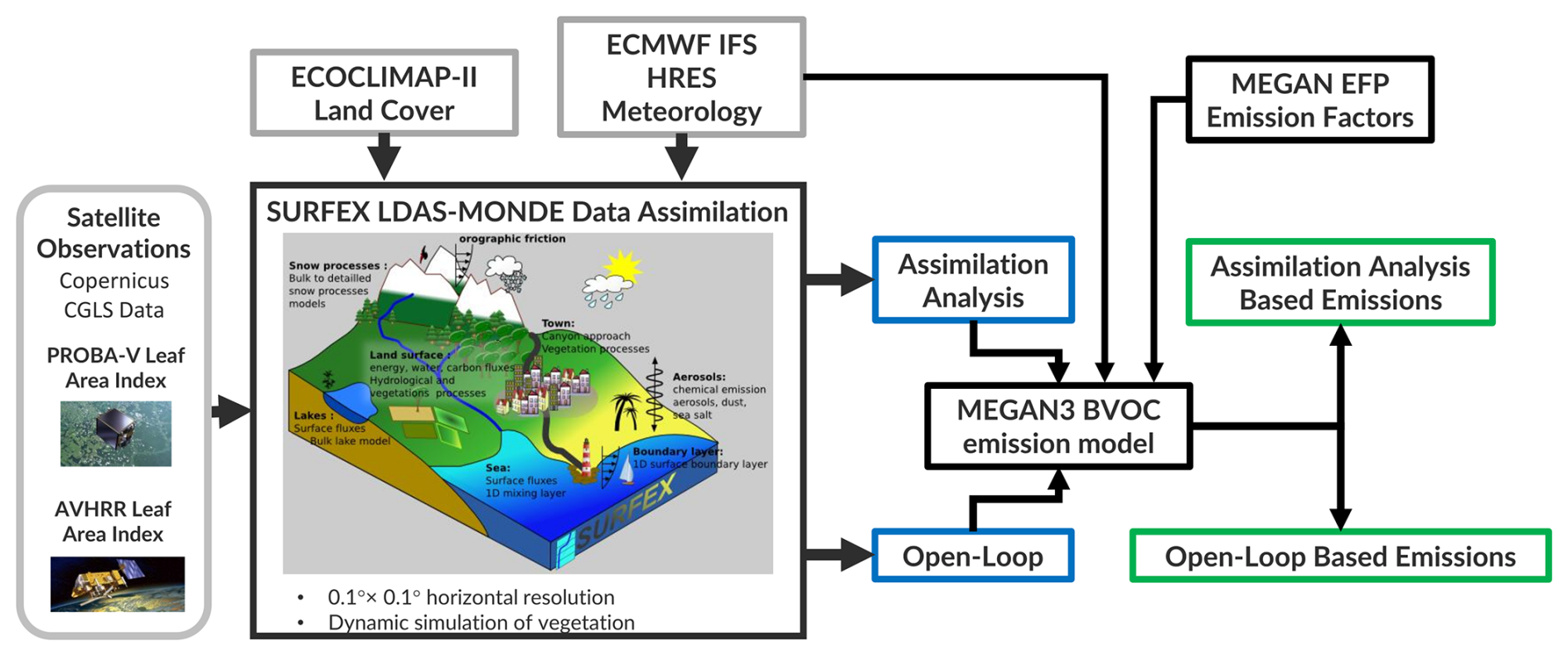
Figure 1 A flow diagram showing how the different modelling elements within this BVOC modelling framework link together. Model components are shown in the black boxes, external input data sources are shown in grey boxes, intermediate data sources are shown in blue boxes, and output data are shown in green boxes. There are three data flows (ECMWF HRES meteorology, ECOCLIMAP-II land surface cover, and satellite observations of LAI based on PROBA-V and AVHRR data) into the SURFEX LDAS-Monde land surface modelling and data assimilation system. The output from SURFEX serves as the inputs into MEGAN3.0. There are two additional dataflows into the MEGAN3.0 model, which are emission factors calculated by the MEGAN EFP and the ECMWF HRES meteorology. We produce two differing BVOC emission datasets (open-loop and assimilation analysis) based on the corresponding output datasets from SURFEX of each type.

2.2 The MEGAN 3.0 Emission model

2.2.1 Model overview

We first provide an overview of the basic conceptual framework built within MEGAN3.0 (Guenther et al., 2020). This concept can be described in a simple equation defining the net emission flux into the above-canopy atmosphere of species, i as, F_i.

$$\begin{array}{}\text{(1)}& F_i={\mathit{\gamma }}_i\times \sum _{k=\mathrm{1}}^n({\mathit{\epsilon }}_{i,k}\times {\mathit{\chi }}_k)\end{array}$$

Here, γ_i is the chemical species-specific activity, ε_i,k is the emission factor at standard conditions for vegetation type k, and χ_k is the fractional grid box areal coverage. The activity represents changing environmental conditions (e.g., air temperature and radiation) and vegetation properties (e.g., LAI) that impact BVOC emissions. Activity is calculated by multiplying a set of different γ activity parameters together in series (explained in more detail in Sect. 2.2.2) where each parameter represents a different process impacting activity. The emission factors are a measure of the potential emissions of a particular compound from a specific plant type. As a whole, this conceptual framework is expressed via algorithms within a software package containing the MEGAN3.0 model (consisting of five sub-components) and as well a separate MEGAN emission factor pre-processor (MEGAN EFP). We provide a schematic diagram in Fig. 2 giving an overview of MEGAN3.0 and its five sub-components, the MEGAN EFP, the dependencies on external data sources at each step, and the sequential steps used in the production of the intermediate datasets that all eventually lead to the final output BVOC emissions. These intermediate datasets are associated with specific environmental processes that impact activity (e.g., soil moisture) as well as physical properties affecting leaf physiology, e.g., temperature and radiation.

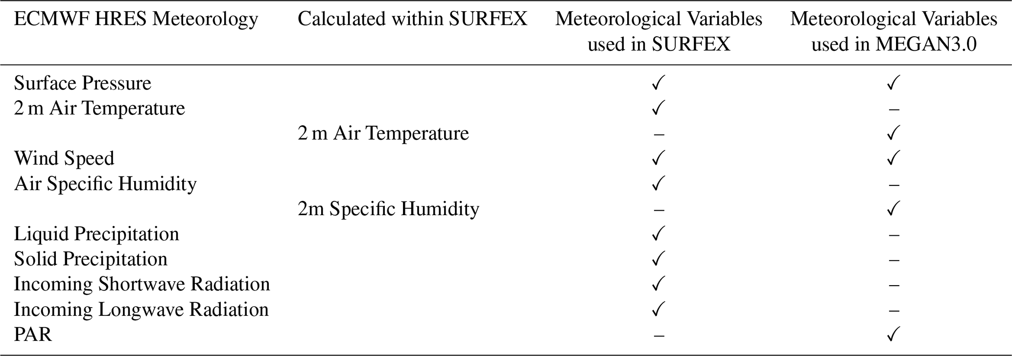
We now describe the five sub-components of MEGAN3.0 in turn. The first is DAYMET, which calculates daily meteorological parameters using ECMWF (in our case) wind speed and accumulated photosynthetically active radiation (PAR), and 2 m-temperature from the SURFEX land surface model. DAYMET calculates the daily mean, minimum, and maximum temperature, the daily mean photosynthetic photon flux density (PPFD), and the maximum daily wind speed.

The second sub-component is CANMET, which is a canopy meteorological model that calculates shaded and sunny leaf temperatures and PPFDs for different vertical layers in the vegetation canopy as well as the fraction of sunny leaves at each canopy layer height. CANMET is important for calculating the transmission of solar radiation into the lower layers of the of dense canopy when LAI is high, i.e., > 3 m⁻² m⁻². In the configuration used in the SEEDS project, CANMET uses wind speed, surface pressure and accumulated PAR from ECMWF's IFS HRES data, and 2 m-temperature and 2 m-specific humidity calculated within SURFEX.

The third sub-component within MEGAN3.0 is MEGSEA, which is responsible for calculating the effects of soil physical properties estimated by the SURFEX land surface model (root zone soil moisture and root zone soil temperature) on BVOC and soil NO_x emissions. The outputs from MEGSEA are the soil moisture activity parameter, γSM, and the soil NO_x activity parameter, which are both dependent on soil moisture and are sensitive to drought effects.

The fourth sub-component is MEGVEA, which uses parameters calculated by the preceding sub-components (DAYMET, CANMET, and MEGSEA) to calculate all of the remaining activity parameters (more details in Sect. 2.2.2) associated with different physical and biological processes. The code then calculates the product of all of these parameters to then calculate and output the activity for a range of aggregated BVOC species.

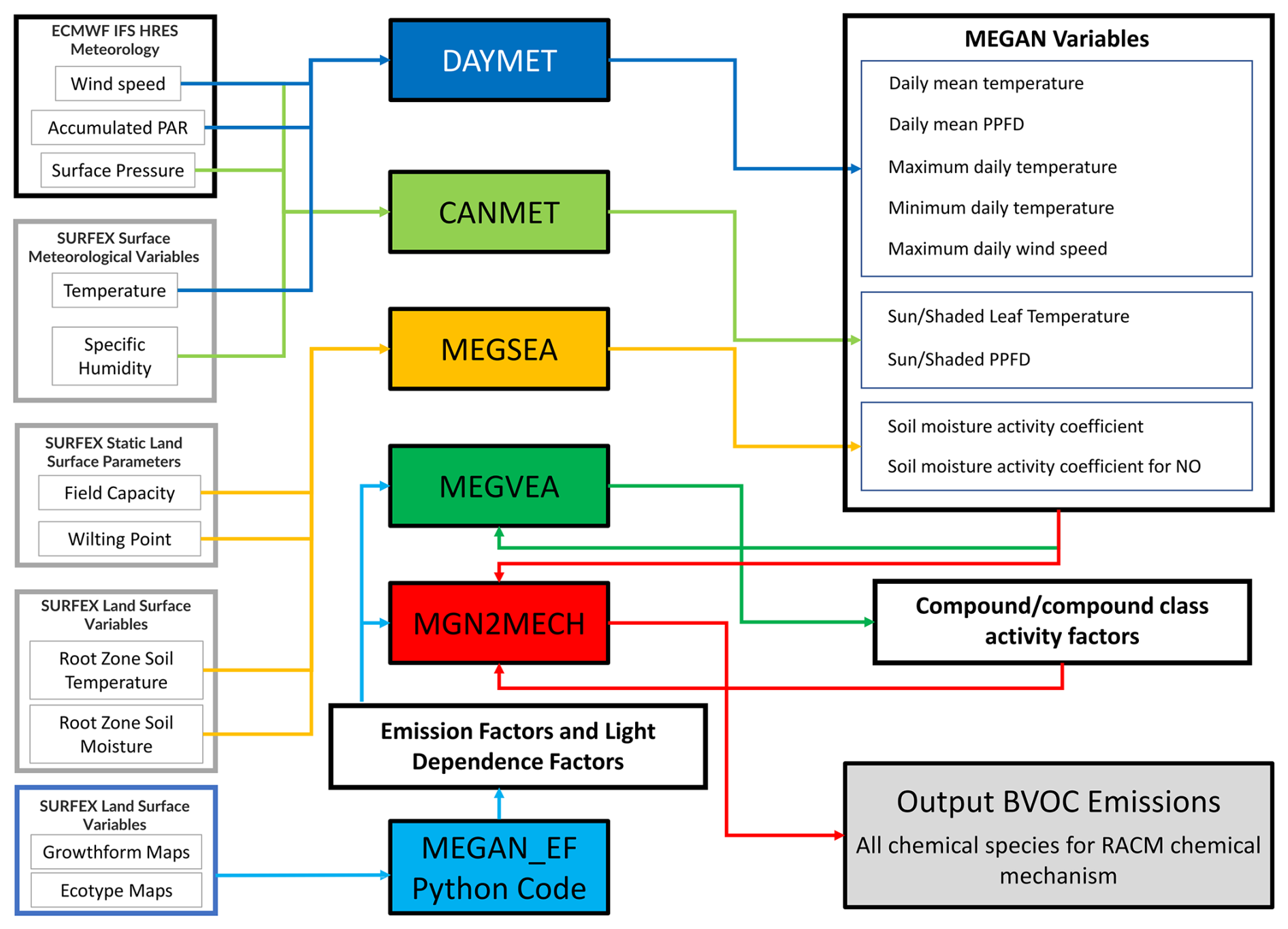
Figure 2 A detailed flow diagram of the MEGAN3.0 BVOC emission model as used in our application. The five modelling components of MEGAN3.0 are shown in the coloured boxes (DAYMET in dark blue, CANMET in light green, MEGSEA in orange, MEGVEA in dark green, MGN2MECH in red). Note that MEGAN3.0 has to be run sequentially in this order. The MEGAN emission factor pre-processor shown in a light blue box must be run prior to the final MEGAN3.0 step (MGN2MECH). Note that the input and output flows for each model sub-component are represented using corresponding colour coded arrows. The various intermediate inputs and outputs are shown in light grey boxes. Lastly, the output BVOC emissions calculated by MEGAN3.0 from the MGN2MECH routine are shown in the grey-filled box.

Prior to describing the final sub-component of MEGAN3.0 it is appropriate to briefly describe MEGAN EFP. MEGAN EFP calculates the emission factors and light-dependent factors over the chosen spatial grid using a set of maps of plant ecotype and growth form as input. The calculation of the emission factors and the MEGAN EFP software package are described in more detail in Sect. 2.2.3.

The final sub-component with MEGAN3.0 is MGN2MECH. MGN2MECH performs a dual function. First, it calculates the emissions of BVOCs by multiplying the emission factors and activity according to Eq. (1). Second, it performs a reaggregation of the BVOC emissions to derive an output emissions dataset that is compatible with the selected chemical mechanism. In our example case this is for the RACM chemical mechanism (Stockwell et al., 1997). The chemical species associated with RACM mechanism that are included in the datasets are described in detail in Table S1 in the Supplement.

2.2.2 Emission Activity

The activity, γ_i, represents the vegetation BVOC emission response to changing environmental conditions. γ_i is calculated by multiplying together a series of other parameters that represent vegetation properties and responses to changing environmental conditions. We describe how γ_i is calculated for different chemical species and then describe how the parameters most relevant to this study (g_TP and g_SM) are calculated.

We define the standard activity that applies to the generic chemical species defined within MEGAN3.0 (i.e., this excludes isoprene, ethanol, acetaldehyde, and carbon monoxide) as:

$$\begin{array}{}\text{(2)}& {\mathit{\gamma }}_i=\mathrm{LAI}\times {\mathit{\gamma }}_{\mathrm{TP}}\times {\mathit{\gamma }}_{\mathrm{LA}}\times {\mathit{\gamma }}_{\mathrm{HW}}\times {\mathit{\gamma }}_{\mathrm{AQ}}\times {\mathit{\gamma }}_{\mathrm{HT}}\times {\mathit{\gamma }}_{\mathrm{LT}}{\times }_{\mathrm{SM}}\times \mathrm{LDF}\end{array}$$

Here, the activity used for BVOC chemical species that have a generic response are γ_TP, which is the canopy average temperature and radiation response parameter, γ_LA is the leaf age response parameter, γ_HW is the response to high windstorms parameter, γ_AQ is the response to air pollution (ozone) parameter, γ_HT is the response to high temperature parameter, γ_LT is the response to low temperature parameter, γ_SM is the soil moisture response parameter, and LDF is the light dependent fraction (the LDF is explained further in Sect. 2.2.3).

Next, we first define the emission activity for isoprene as:

$$\begin{array}{}\text{(3)}& \begin{array}{rl}{g}_{\mathrm{isoprene}}& =\mathrm{LAI}\times {\mathit{\gamma }}_{\mathrm{TP}}\times {\mathit{\gamma }}_{{\mathrm{CO}}_{\mathrm{2}}}\times {\mathit{\gamma }}_{\mathrm{LA}}\times {\mathit{\gamma }}_{\mathrm{HW}}\times {\mathit{\gamma }}_{\mathrm{AQ}}\\ & \times {\mathit{\gamma }}_{\mathrm{HT}}\times {\mathit{\gamma }}_{\mathrm{LT}}\times {\mathit{\gamma }}_{\mathrm{SM}}\times \mathrm{LDF}\end{array}\end{array}$$

Where ${\mathit{\gamma }}_{{\mathrm{CO}}_{\mathrm{2}}}$ defines the carbon dioxide response, which is only relevant for isoprene and thus makes the isoprene emission activity slightly different from all of the other chemical species. Next, we define the activity for ethanol and acetaldehyde:

$$\begin{array}{}\text{(4)}& \begin{array}{rl}& {\mathit{\gamma }}_{\text{ethanol\hspace{0.17em} or\hspace{0.17em} acetaldehyde}}=\mathrm{LAI}\times {\mathit{\gamma }}_{\mathrm{TP}}\times {\mathit{\gamma }}_{\mathrm{BD}}\times {\mathit{\gamma }}_{\mathrm{LA}}\times {\mathit{\gamma }}_{\mathrm{HW}}\\ & \times {\mathit{\gamma }}_{\mathrm{AQ}}\times {\mathit{\gamma }}_{\mathrm{HT}}{\times }_{\mathrm{LT}}\times {\mathit{\gamma }}_{\mathrm{SM}}\end{array}\end{array}$$

Where γ_BD is the bidirectional exchange LAI response parameter, which is only relevant for both ethanol and acetaldehyde. The definition of the emission activity for carbon monoxide also differs from that of the other chemical species:

$$\begin{array}{}\text{(5)}& {\mathit{\gamma }}_{\mathrm{CO}}=\mathrm{LAI}\times {\mathit{\gamma }}_{\mathrm{TP}}\times {\mathit{\gamma }}_{\mathrm{LA}}\times {\mathit{\gamma }}_{\mathrm{HW}}\times {\mathit{\gamma }}_{\mathrm{AQ}}\times {\mathit{\gamma }}_{\mathrm{HT}}\times {\mathit{\gamma }}_{\mathrm{LT}}\times {\mathit{\gamma }}_{\mathrm{SM}}\end{array}$$

We now describe the equations defining the two activity parameters of interest to this work in turn. The canopy average temperature and radiation response parameter, γ_TP, is calculated via:

$$\begin{array}{}\text{(6)}& {\mathit{\gamma }}_{\mathrm{TP}}=\sum _{j=\mathrm{1}}^{j=\mathrm{5}}\left({\mathit{\gamma }}_{{\mathrm{TP}}_{\mathrm{LDF}}}^j\times \mathrm{LDF}+{\mathit{\gamma }}_{{\mathrm{TP}}_{\mathrm{LIF}}}^j\times (\mathrm{1}-\mathrm{LDF})\right)\times W^j\end{array}$$

where W^j are the predefined layer-specific weights distributing the potential emission across the different canopy layers and are defined as follows: 0.119, 0.239, 0.284, 0.239, and 0.119. These weights implicitly assume the vertical structure of the canopy follows this prescribed definition. The light-dependent fraction temperature and radiation response g_TP is calculated for each layer, j, within the canopy via:

$$\begin{array}{}\text{(7)}& \begin{array}{rl}{\mathit{\gamma }}_{{\mathrm{TP}}_{\mathrm{LDF}}}^j& =({\mathit{\gamma }}_{\mathrm{CD}}^j\times {\mathit{\gamma }}_{{\mathrm{TLD}}_{\mathrm{sun}}}^j\times {\mathit{\gamma }}_{{\mathrm{P}}_{\mathrm{sun}}}^j\times f_{\mathrm{sun}}^j)\\ & +({\mathit{\gamma }}_{{\mathrm{TLD}}_{\mathrm{shade}}}^j\times ({\mathit{\gamma }}_{{\mathrm{P}}_{\mathrm{shade}}}^j\times (\mathrm{1}-f_{\mathrm{sun}}^j))\end{array}\end{array}$$

Here, γ_P is the light response parameter, which is calculated independently for sunlit and shaded leaf areas depending on the photon flux within the canopy (calculated by CANMET – see Sect. 2.2.1) for both sunlit and shaded areas. γ_TLD is the light dependent temperature response parameter, which is also calculated independently for sunlit and shaded leaf areas. $f_{\mathrm{sun}}^j$ is the fraction of sunlit area at each canopy layer height and g_CD is the canopy depth parameter.

The light-independent fraction temperature and radiation response parameter for each canopy layer is defined as:

$$\begin{array}{}\text{(8)}& {\mathit{\gamma }}_{{\mathrm{TP}}_{\mathrm{LIF}}}^j=({\mathit{\gamma }}_{{\mathrm{TLI}}_{\mathrm{sun}}}^j\times f_{\mathrm{sun}}^j)+\left({\mathit{\gamma }}_{{\mathrm{TLI}}_{\mathrm{shade}}}^j\right(\mathrm{1}-f_{\mathrm{sun}}^j\left)\right)\end{array}$$

γ_TLI is the light independent temperature response activity parameter, which is calculated separately for sunlit and shaded areas to take into account the differences in leaf surface temperature in both regions of the canopy at a particular layer height.

The soil moisture activity factor, g_SM, is calculated differently according to whether the soil moisture, q, satisfies one of three different conditions:

$$\begin{array}{}\text{(9)}& \begin{array}{rl}& {\mathit{\gamma }}_{\mathrm{SM}}=\mathrm{0}q<q_{\mathrm{wilt}}\\ & {\mathit{\gamma }}_{\mathrm{SM}}=q-q_{\mathrm{wilt}}/\mathrm{0.04}{q}_{\mathrm{wilt}}\le q\le q_{\mathrm{wilt}}+\mathrm{0.04}\\ & {\mathit{\gamma }}_{\mathrm{SM}}=\mathrm{1}{q}_{\mathrm{wilt}}<q\end{array}\end{array}$$

Where q_wilt is the wilting point taken from the SURFEX physio-geographic maps, which is volumetric soil moisture at which plants are defined to wilt in SURFEX for a particular location.

The γ_HW, γ_AQ, γ_HT, and γ_LT activity factors are calculated with an approach that is similar to the above equation for the soil moisture activity factor. For the remaining activity parameters we refer readers to Guenther et al. (2012), which describe the details of how γ_LA and ${\mathit{\gamma }}_{{\mathrm{CO}}_{\mathrm{2}}}$ are calculated.

2.2.3 Emission Factors

The MEGAN EFP is built on the Python programming language with the SQLite database system as an opensource program that generates the emission factor and light dependence factors (EF/LDFs) required to drive MEGAN3.0. The program first generates EF/LDFs for individual plant types and then integrates them with plant type distribution data to calculate landscape-average EF/LDFs for a modelling domain.

To generate EF/LDFs for individual plant types, emission factor measurements compiled in the MEGAN EFP database are assigned a number from 0 to 4, called the J-rating, to indicate the quality of the data. A J-rating of 0 indicates the lowest quality including qualitative measurements and measurements conducted with methods that have high uncertainties and potentially strong bias. A J-rating of 4 is the highest quality data indicating that the data were obtained using methods that meet the recommendations of the BVOC emission measurement community (e.g., Niinemets et al., 2011). The MEGAN EFP allows users to choose to use all data or just measurements higher than a specified minimum J-value. The MEGAN EFP database also contains specific leaf area data (SLA) to convert EF measurements reported in terms of emissions per unit leaf mass to emissions per unit leaf area which is used by MEGAN.

Landscape average EF/LDFs are calculated with the MEGAN EFP by synthesizing leaf level plant trait data, including BVOC emission factors, specific leaf area and emission light dependence factor, with landcover data (described in more detail shortly), including ecotype and growth-form fractions for each location in a modelling domain. Additional information in the MEGAN EFP database includes descriptions of biogenic compounds, emission classes, publication references, vegetation types, and canopy vertical distribution characteristics. These data allow users to identify the emissions data that were used to drive the MEGAN3.0 model emission inputs.

We now describe the landcover data used by MEGAN EFP in more detail. The MEGAN3.0 emission factor distributions are based on four landcover input types: growth form fractions, ecotypes, plant type composition, and plant type emission factors. The growth form fractions, and ecotype inputs are ∼ 1 km² (30 s latitude × 30 s longitude) resolution global maps. The growth forms include trees, which are further divided into broadleaf vs needleleaf trees and tropical and extratropical trees, shrubs, grass and other herbaceous plants and crops. The total vegetation cover was based on a twelve-year climatology (Broxton et al., 2014) and the relative fractions from global datasets of tree cover (Hansen et al., 2003), shrub and grass cover (Tuanmu and Jetz, 2014) and crop cover (Latham et al., 2014) that were merged with regional data including the NLCD 30-meter landcover data for the U.S. (Homer et al., 2015). The ecotypes include ∼ 900 global ecotypes and ∼ 1200 regionally specific ecotypes for the U.S. and Australia (Guenther et al., 2012) and ∼ 400 locally specific ecotypes representing specific U.S. cities and urban neighborhoods.

The plant type composition data is specified for each growth form and ecotype. For example, the plant type composition for a pine-oak forest ecotype includes the plant type composition for each growth form including broadleaf trees (dominated by oaks), needleleaf trees (dominated by pines), grass (temperate woodland grass), shrub (temperate woodland grass) and crop (generic crop). The plant types range from very specific, such as a plant species or even subspecies, to general types such as broadleaf tropical rainforest tree or arctic grass. The final database contains emission factors for each of the 20 MEGAN3.0 emission categories for each plant type. The four input data types were used to estimate weighted average emission factors at each location. The emission factors were based on data compiled for MEGAN2.1 (Guenther et al., 2012) with updates for vegetation in parts of the U.S. and Australia based on locally specific data.

2.3 Land surface model data

We use ISBA (Interactions Between Soil, Biosphere, Atmosphere) within the SURFEX (SURface EXternalisée) modelling platform (Masson et al., 2013) in this work to provide some of the key land surface variables (i.e., 2 m-specific humidity, 2 m-temperature, root zone soil temperature, root zone soil moisture, LAI) used in MEGAN. SURFEX simulates heat, moisture, and gas fluxes at the atmosphere-surface boundary and is designed to be coupled with meteorological models and atmospheric forcing both online and offline, respectively. SURFEX has been used successfully in a wide range of applications, e.g., river discharge prediction (Fairbairn et al., 2017), drought monitoring (Albergel et al., 2019), and urban climate studies (Schoetter et al., 2020). Regarding the soil-plant system, ISBA can simulate changes in Leaf Area Index (LAI) according to how meteorology impacts on the growing season. It has been shown to be skilful at estimating phenological changes and soil moisture on seasonal timescales when forced with state-of-the-art meteorological atmospheric forcing (Albergel et al., 2019; Szczypta et al., 2014).

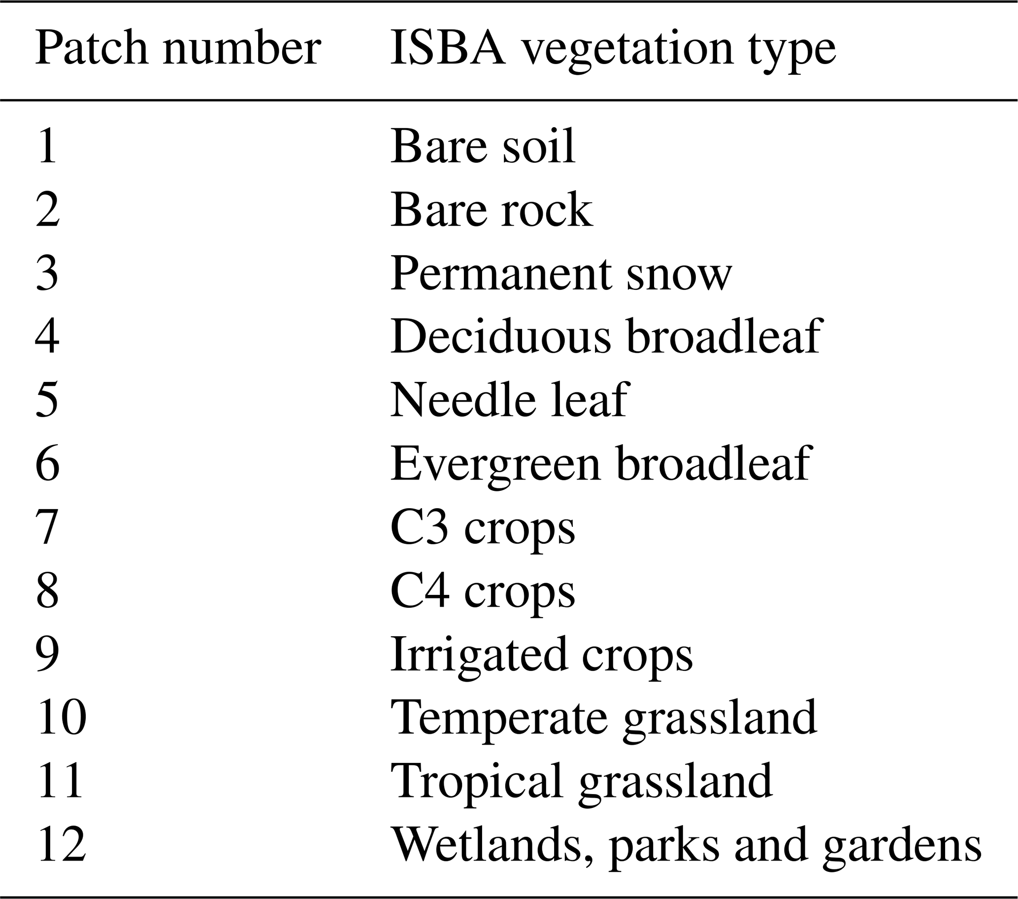
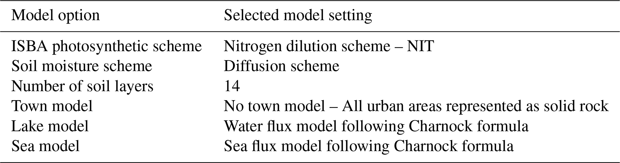
SURFEX simulates four broad land use classes, nature, town, fresh water (lakes, rivers, and lagoons), and sea (see schematic embedded within Fig. 1). The nature type is represented within SURFEX by 12 sub-classes of land surface class that represent different types of biomes and agricultural land use. These different land surface types and sub-classes are defined by ECOCLIMAP-II (Faroux et al., 2013). These 12 sub-classes are listed in Table 1. SURFEX was run using 12 sub-classes (termed patches) of the nature land type because some of the model options (detailed below in Table 2) that are required to run simulations of vegetation phenology can only be run with these 12 patch types. Table 2 summarises all of the relevant model options used.

Table 1 List of SURFEX nature tile patch numbers and corresponding ISBA vegetation type.

SURFEX was configured to run on the same 0.1° × 0.1° spatial grid we use for MEGAN3.0, which is the same spatial domain as used by the CAMS regional air quality models and the ECMWF HRES meteorology. The meteorological parameters required by SURFEX were retrieved from ECMWF onto this spatial grid. While this increased high spatial resolution has been already used in applications for specific isolated domains within Europe (Albergel et al., 2019), this is the first time SURFEX LDAS-MONDE will be run for the whole of Europe at this high spatial resolution.

Table 2 Model options used in SURFEX.

SURFEX also includes a capability to perform data assimilation of satellite observations of land surface variables (soil moisture and LAI) using the Simplified Extended Kalman Filter (see e.g., Albergel et al., 2017). In this configuration SURFEX is termed the SURFEX LDAS-Monde (Land Data Assimilation System-World/Global), which can be applied with relative ease to study any area of the world. Assimilation of satellite observations of LAI and soil moisture in SURFEX LDAS-Monde has been shown to improve estimates of the soil moisture content and of phenological changes (Albergel et al., 2017) with LAI having a more significant and beneficial effect for the estimation of root zone soil moisture. For the purposes of the production of the BVOC emission datasets presented in this article we produce two different sets of land surface data for use in MEGAN. The first is just SURFEX run in a free-running mode with no data assimilation, which we term the open-loop dataset. The second is a SURFEX simulation run created by running SURFEX with data assimilation of satellite LAI, which we term the analysis. The analysis is run with the aim to improve estimation of LAI and the root zone soil variables that are relevant for vegetation growth and function that are used in MEGAN, i.e., root zone soil moisture and root zone soil temperature.

To produce the assimilation-based analysis we assimilate LAI satellite data products from the Copernicus Land Monitoring Service (CLMS, https://land.copernicus.eu/en/products/vegetation?tab=vegetation_properties, last access: 17 July 2025). Specifically, this includes assimilation of the PROBA-V LAI (Verger et al., 2014; Fuster et al., 2020) product for years 2018 and 2019, using the GEOV1 product of CGLS. Since PROBA-V was decommissioned in 2020, we used the THEIA AVHRR-derived LAI (https://geodes-portal.cnes.fr/, last access: 24 April 2026) and performed a seasonal cumulative density function (CDF) matching of the latter from 1999 to 2019 (21 years) in order to use the CDF-matched THEIA LAI as a proxy of GEOV1 for the whole 2020. This AVHRR LAI product is derived from the Land Long Term Data Record (LTDR) AVHRR data (Roger et al., 2021) (https://landweb.modaps.eosdis.nasa.gov/data/userguide/ LTDR_Ver5_Products_UserGuide_v1.0.pdf, last access: 17 July 2025) using another version of the GEOV2-AVHRR algorithm described in Pacholczyk and Verger (2020) (https://www.theia-land.fr/wp-content/uploads/2022/03/THEIA-MU-44-0369-CNES-GEOV2-AVHRR-Product-User-Manual-V2_AV.pdf, last access: 17 July 2025).

We did not use the CLMS LAI products for LAI from Sentinel-2 or from Sentinel-3 because we did not need the higher resolution of Sentinel-2 in this application, and we found a discontinuity between the PROBA-V and the Sentinel-3 data version that was available at the time of study.

2.4 Meteorology

Both the SURFEX and MEGAN3.0 model algorithms rely on the use of meteorological data from the European Centre for Medium-Range Weather Forecasts (ECMWF) HRES operational forecast (Owens and Hewson, 2018) for describing the meteorological conditions. The data was extracted via the MARS service (ECMWF's Meteorological Archival and Retrieval System) on a 0.1° × 0.1° grid with hourly resolution for the surface levels. The forecast at 12:00 was used and the following 36 h have been retrieved and then post-processed to create a single contiguous daily time series running from the 13th hour of the forecast (00:00 UTC) to the 36th hour (23:00 UTC). We then combined each individual daily time series together to make a continuous running time series spanning the full dataset time period, i.e., 2018–2022. Table 3 shows which meteorological variables were extracted for use in which of the two models (SURFEX and MEGAN3.0). In the case of MEGAN3.0 we used two of the variables (2 m air temperature and 2 m specific humidity) calculated by SURFEX. There is a specific advantage to using these variables from SURFEX as opposed to the ECMWF HRES data directly because SURFEX can account for surface effects like surface fluxes of latent and specific heat and surface driven turbulence arising from different vegetation canopy heights and densities and different transpiration rates. In the case of all other meteorological variables the models used ECMWF HRES data.

We used the ECMWF HRES forecast as opposed to ECMWF's ERA5 reanalysis (Hersbach et al., 2020) in this study for several reasons. The CAMS European production runs at a spatial resolution of 0.1° × 0.1°, which corresponds to the spatial resolution of the HRES forecast. Furthermore, some of the CAMS models use the HRES forecast on its native gridding. An important aim was to try to follow the gridding used by HRES to facilitate testing of the emissions in the CAMS models. ERA5 reanalysis with its spatial resolution of 0.25° × 0.25° was, therefore, unsuitable for this purpose. Next, since the land surface has a high degree of heterogeneity, operating a land surface model at higher resolution allows one to represent this heterogeneity in a more thorough way within the model. This can be important, for instance, to represent which particular land covers/vegetation types receive rainfall. This was explored by (Jarlan et al., 2023) who concluded that higher spatial resolution forcing improved drought monitoring over specific affected areas/vegetation and improved the representation of its effects on vegetation. Lastly, coarser model spatial resolutions have downstream effects on the assimilation of LAI data. Coarser resolutions mean that satellite LAI data has to be spatially aggregated even more, which degrades the effectiveness of the assimilation step due to broadening of the number of land use classes within larger spatial pixels.

Table 3 Summary of meteorological variables used as inputs by the SURFEX and MEGAN3.0 algorithms.

2.5 Isoprene Observations

We perform an evaluation of the temporal variability of the BVOC emissions using in-situ observations of isoprene collected during the period of our datasets (2018–2022). We obtained the isoprene observations from the EBAS database (Europe-wide observations excluding UK; EBAS home – ebas homepage, https://ebas.nilu.no/, last access: 17 July 2025) and from UK-air (specific to UK observations; Data Archive – Defra, UK, https://uk-air.defra.gov.uk/data/, last access: 17 July 2025). The isoprene data from Beromunster (https://doi.org/10.48597/9M6N-7GJZ, Hill and Reimann, 2026) and Hohenpeissenberg (Plass-Dülmer et al., 2002) (https://doi.org/10.48597/V8XG-29XA, Claude and Kubistin, 2026) include the use of data affiliated with the frameworks: GAW-WDCRG, ACTRIS, and EMEP. The isoprene data from Zurich-Kaserne (https://doi.org/10.48597/UYW4-RZPY, Hill et al., 2026) includes the use of data affiliated with the frameworks: GAW-WDCRG, RI-URBANS, EMEP, and ATMO-ACCESS. The isoprene data from Feyzin Stade and Vernaison were sourced from Atmo Auvergne-Rhône-Alpes. The data from Auchencorth and Eltham were funded and collected on behalf of the UK Environment Agency. The EBAS database contains a wide variety of isoprene observations collected using different monitoring techniques. We select only observations made using the online gas chromatograph based method and we made a further selection to exclude observations made in dense urban settings, e.g., Marylebone Road, London, to avoid sites with a strong influence from anthropogenic isoprene sources (Khan et al., 2018).

3 Results and Discussion

We describe different aspects of the SURFEX-MEGAN3.0 datasets within the following three sub-sections. First, in Sect. 3.1, we perform an evaluation of the underlying LAI data produced in the course of running the SURFEX-MEGAN3.0 production chain. Then, in Sect. 3.2, we describe the spatiotemporal characteristics of the datasets and we describe the impact of the LAI data assimilation on the results. Lastly, we evaluate the SURFEX-MEGAN3.0 emission inventory for isoprene against other published emission inventories in Sect. 3.3. Throughout these discussions we focus on isoprene emissions. Isoprene is one of the most important BVOCs because its emissions are larger than other emitted BVOC species and it is one of the most reactive BVOCs and it therefore has an important influence on atmospheric composition.

3.1 Performance of SURFEX land surface model

One important conceptual basis for the creation of the BVOC emission datasets presented in this paper was that we could improve BVOC emission modelling by focusing on improvements of the input data used by the MEGAN emission model. Indeed, we hypothesize that BVOC emission modelling can be advanced by using the SURFEX land surface model to provide improved estimates of LAI and soil moisture based on realistic vegetation phenology. Furthermore, we posit that the inclusion of the methodological step to assimilate satellite observations of LAI further improves the model representation of LAI used for BVOC estimation. Thus, we now attempt to evaluate the performance of the SURFEX land surface model for these key input variables used by MEGAN. We perform this evaluation using four approaches: (i) a review and discussion of literature covering existing case studies evaluating the performance of the SURFEX land surface model, (ii) a brief review of the data quality of the LAI satellite observations used, (iii) the use of TROPOMI satellite observations of solar induced fluorescence (SIF) (Guanter et al., 2021) to evaluate LAI, and (iv) in-situ observations of soil moisture. In addition, we refer readers to Sect. 3.2.2 that covers a discussion of the impacts of the assimilation of satellite observations of LAI as this gives some further insight into the relative performance of the OL and analysis model runs.

Unlike other land surface models, phenology in ISBA is entirely driven by photosynthesis and LAI responds to environmental factors such as drought, temperature, or solar radiation through photosynthesis (Calvet et al., 1998; Gibelin et al., 2006). ISBA is not calibrated and the vegetation parameters that drive photosynthesis and plant growth are derived from the literature (Delire et al., 2020). Despite this unique way of representing phenology, ISBA can achieve good skill compared to other LSMs (Peano et al., 2020; Friedlingstein et al., 2022).

The CLMS LAI data assimilated by SURFEX has been evaluated extensively (Brown et al., 2020; Sanchez-Zapero et al., 2018; Verger et al., 2023) demonstrating its consistency with MODIS products, temporal consistency, and highest accuracy when compared to reference data. Thus, the LAI data ingested into the SURFEX assimilation algorithm has an established track record of being of high quality.

To assess the correlation between the SIF observations and both the LAI open-loop and LAI analysis, temporal correlation coefficients with SIF and LAI are calculated over the entire domain from 1 May 2018 to 31 December 2020. The LAI and SIF data are compared on a time frequency dependent on the availability of the TROPOMI SIF data. The TROPOMI SIF data were the limitation in this case because the SURFEX model provided OL and analysis data continuously for every day with no data gaps. In practice the TROPOMI data were available for approximately 25 d in every month on average even though the SIF observations are nominally available once per day. The limitation is due to data gaps created by clouds and viewing angle, which in turn impact the retrieval quality (Guanter et al., 2021). These limitations are more prevalent during the winter months and at higher latitudes. The comparisons are done as and when a model-obs data pair (LAI-SIF) is available.

The results, shown in Fig. 3, show robust correlations over much of the domain with correlation coefficients (R) greater than 0.7 for both the LAI open-loop and LAI analysis. Semi-arid regions such as parts of the Iberian Peninsula and the Middle-East, together with Nordic regions at high latitudes, show weaker correlation values. These regions present sparse vegetation and the SIF signal is weak, which likely degrades the correlations by making the SIF observations more subject to random and systematic errors in the retrieval. Figure 3 also shows the difference in correlation coefficients between the analysis and the open-loop LAI. When comparing the analysis with the OL (Fig. 3b), improvements can be seen over almost the whole study area. In particular, it can be seen that the assimilation improves the correlation between LAI and SIF over Germany and the Czech Republic. It should be noted, however, that the OL LAI does still correlate with SIF in a reasonable way, but the areas where it shows weaker correlation are more widespread.

Figure 3 Maps showing (a) the Pearson correlation in time between the LAI analysis and the observed TROPOMI SIF (re-gridded to the CAMS spatial gridding) for each 0.1° × 0.1° grid cell and (b)the difference in correlation between the LAI analysis and SIF and the LAI open-loop and SIF.

We now analyse the soil moisture represented by the SURFEX model. The SURFEX model soil layer corresponding to the SMOSMANIA in situ measurements at 0.3 m depth is layer 5 (0.2–0.4 m soil layer) (Calvet et al., 2007). This is also the layer that we use to create the root-zone soil moisture (RSZM) dataset used by MEGAN. The OL and analysis root zone soil moisture (RZSM) simulations for layer 5 are compared with observations from the Saint-Felix de Lauragais (SFL) station of the SMOSMANIA network for the study period (1 May 2018 to 31 December 2020) located in the south-west of France. Data from the Saint-Felix de Lauragais were selected and presented here because of the excellent data quality from this site. Unfortunately, the soil moisture sensors at some of the other sites in the SMOSMANIA network have degraded leading to data quality issues. The open-loop, analysis and in situ time series of RSZM are shown in Fig. 4. The temporal patterns of the open-loop and analysis results clearly correlate with the observed seasonal variability of the RZSM, with similar times of rewetting events. The correlation scores are 0.92 and 0.93 for the OL and analysis (all seasons), respectively, and 0.74 and 0.77 (summertime only) for both model versions. The observed RZSM values range between 0.16 and 0.37 m³ m⁻³, while the corresponding variations in the open-loop and analysis simulations show values between 0.25 and 0.46 m³ m⁻³. The larger simulated RZSM values can be explained by differences between the soil properties used in the model, such as porosity, and the local soil properties around the soil moisture probe. Differences between the open-loop and analysis simulations occur during certain periods of the year, such as the autumn of 2019. The vegetation model is sensitive to soil moisture deficit through a soil wetness index corresponding to rescaled volumetric soil moisture between field capacity and wilting point. In this way, a large absolute bias for volumetric soil moisture has little effect on the vegetation response to drought.

In addition to the comparison to the data from Saint-Felix de Lauragais, we carried out an evaluation of SURFEX soil moisture data with data from the other sites in the SMOSMANIA network (eight in total) that had reasonable data quality over the same time period. The results of this evaluation are presented in the Supplement in Figs. S1 to S8 and the correlation statistics between SURFEX and the soil moisture measurements are presented in Table S2. The correlation scores are all above 0.80 for the comparisons with the data from each of these sites.

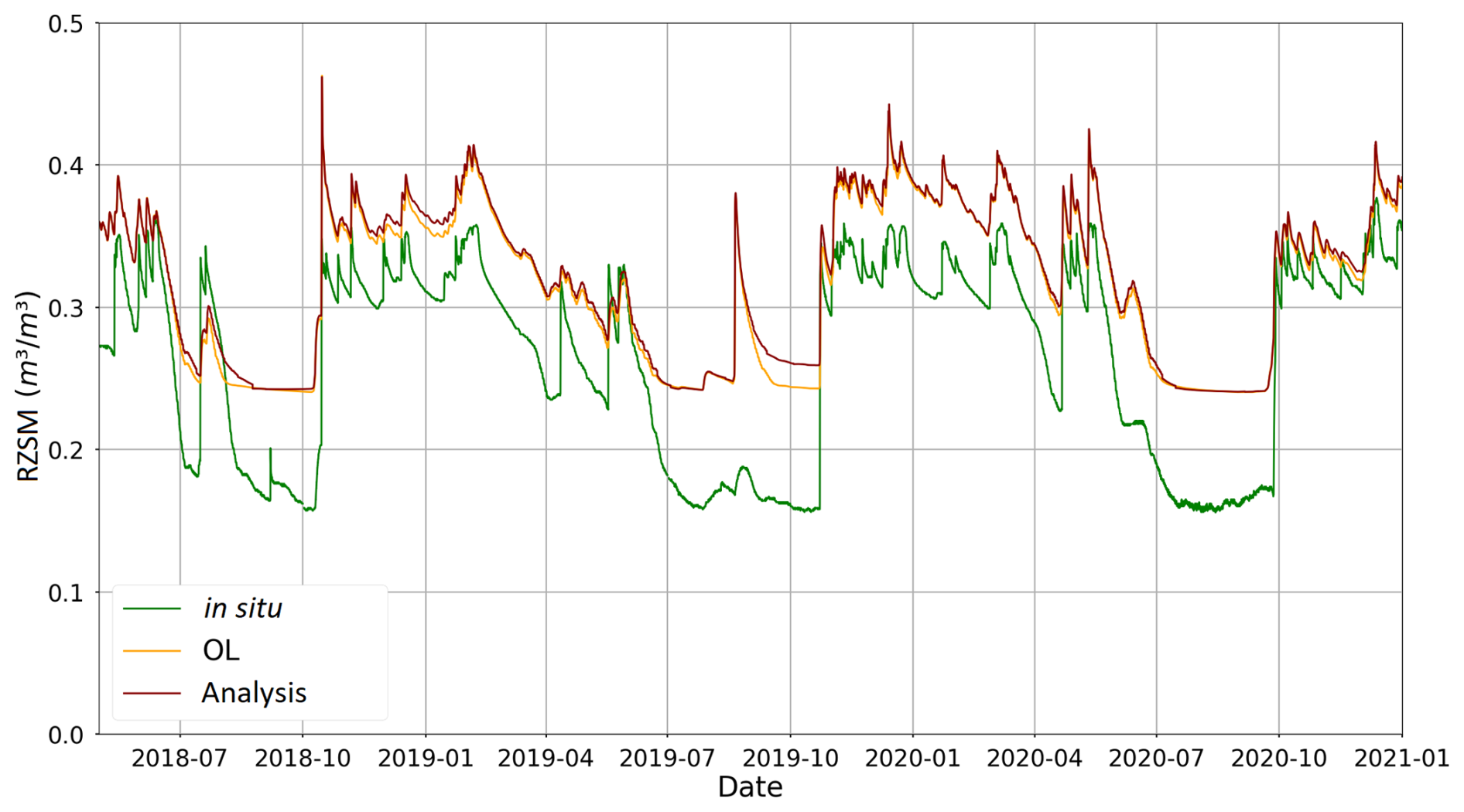
Figure 4 Time series of observed in-situ RSZM at the Saint-Felix de Lauragais SMOSMANIA monitoring station (green), the RSZM from the SURFEX open-loop simulation (yellow), and the RSZM from the SURFEX analysis simulation (red).

In summary, the simulated LAI and RZSM show robust correlations with independent data, and prior work establishes the skill of SURFEX and representing vegetation phenology relative to other LSMs. For LAI, the correlation with SIF is better than 0.7 over much of the domain. However, areas covered by sparse vegetation, semi-arid regions such as parts of Spain, together with Nordic regions at high latitudes, show weaker correlation values.

3.2 Characteristics of SURFEX-MEGAN3.0 BVOC dataset

3.2.1 Spatiotemporal distribution of SURFEX-MEGAN3.0 BVOC emissions over Europe

We first describe the temporal and spatial characteristics of the datasets on an annual basis. The annual mean isoprene emissions are displayed as maps over the CAMS European domain in Fig. 5 for the period 2018–2022. The spatial distribution of the isoprene emissions on an annual scale is dependent on the general distribution of isoprene emitting vegetation as represented in the distribution of the isoprene emission factors. Thus, we see the regions with the highest year-round emissions over areas with dense forest, and the regions with the lowest emissions (near-zero) over desert regions, high mountains, and permanent ice and snow.

The total annual mass of isoprene emissions is shown in Tg above each panel in Fig. 5. The average annual emitted mass of isoprene for the open-loop emissions over the time period 2018–2022 was calculated to be 7.20 Tg yr⁻¹ with a standard deviation of ±0.28 Tg yr⁻¹ over this five year period. The emissions were estimated to be at their highest in 2018 and their lowest in 2020 and the difference in annual emissions between these two extremes was 0.82 Tg yr⁻¹, which represents 11.4 % of the average annual emission of isoprene in this time period. While the standard deviation on the total annual emission over this period is 0.28 Tg yr⁻¹, this temporal variability is not evenly distributed spatially as can be seen within Fig. 6, which shows the standard deviation in isoprene emissions calculated on an inter-annual basis. The areas of highest annual variability over the 2018–2022 period coincide with the co-location of forests, emitting vegetation species, and meteorologically induced variability resulting from temperature, radiation, and soil moisture forcing. Indeed, the effect of these last variables can be seen in more detail within Fig. 7 which shows the emission factors over the CAMS domain and the standard deviation of the inter-annual variability for the gamma activity factors for soil moisture, LAI, and radiation-temperature. Some of the areas with the highest year-to-year variability in emissions correspond to regions over where the emission factors are highest. Since the emission factors are invariant in time, the standard deviation of the emissions will naturally be larger over regions with a higher emission factor as this acts to inflate the variability applied by the parameters used to calculate the activity. Similarly, LAI can vary quite significantly in some regions and where this is co-located with higher emission factors, this can lead to LAI having an important role in modulating emissions, e.g., over France, the Carpathian Mountains, Dinaric Alps, and the Caucasus.

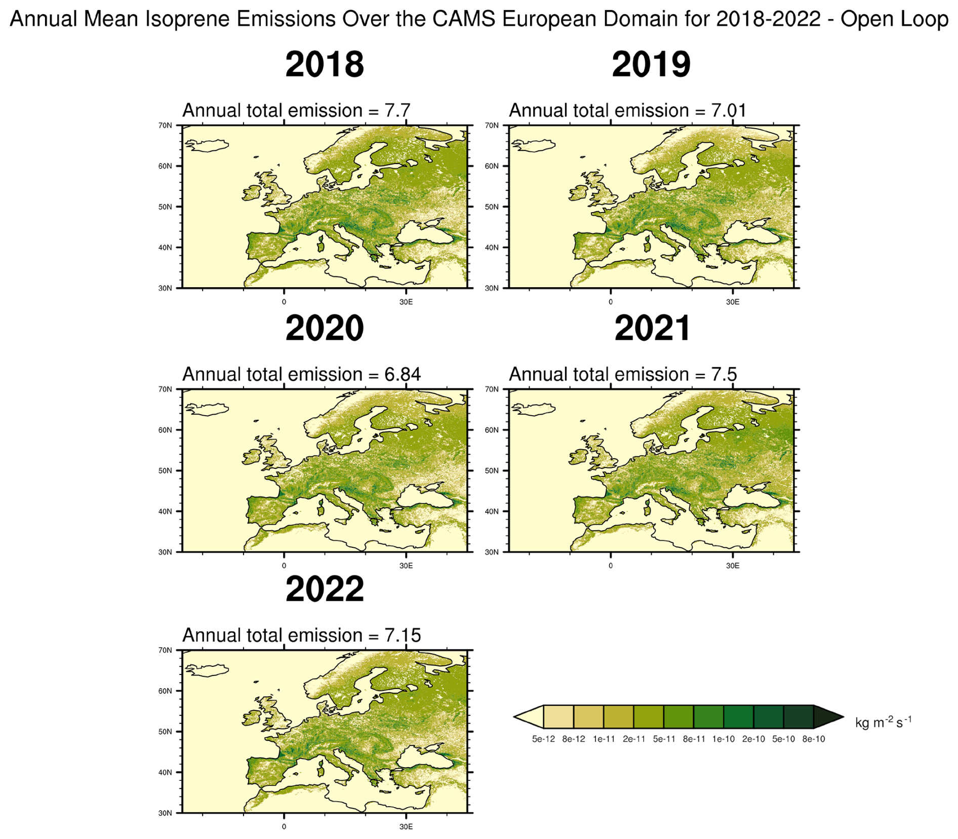
Figure 5 Maps of annual mean isoprene emissions (units of kg m⁻² s⁻¹) calculated using the SURFEX-MEGAN3.0 algorithms over the period 2018–2022 using the open-loop configuration of SURFEX. The panels show each year over this time period moving sequentially from 2018 to 2022 from left to right. The colour bars indicate increasing mean isoprene emissions as the colours transition from pale yellow to dark green. Note that the colour bar has a quasi-logarithmic scale. The annual total mass of isoprene emissions (units of Tg) are shown above each plot.

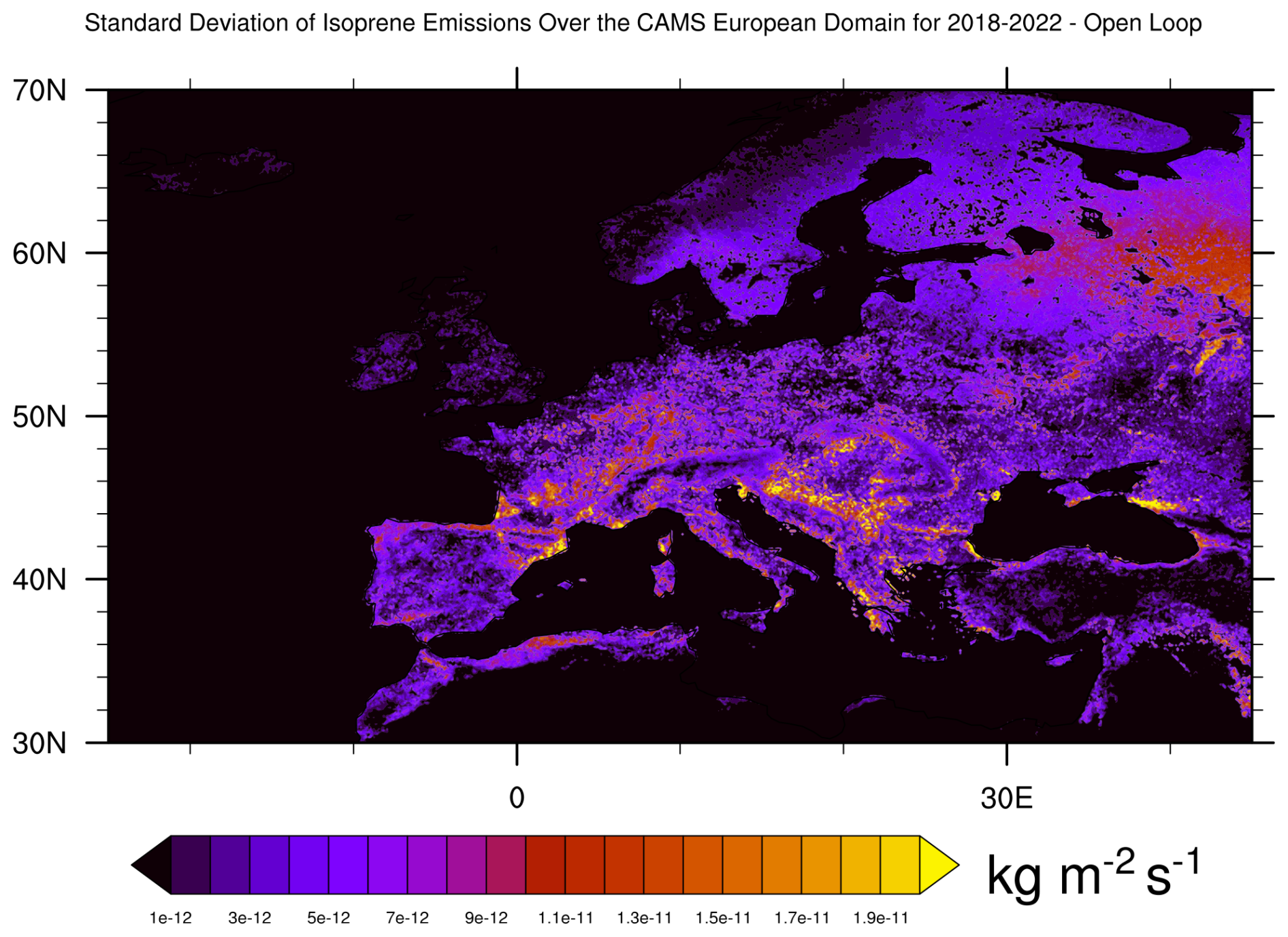
Figure 6 The standard deviation of isoprene emissions over the CAMS European domain for the 2018–2022 period based on the SURFEX model open-loop simulations. Note that the standard deviation is expressed in the units of the emissions (kg m⁻² s⁻¹).

In addition to analysing the standard deviation of the gamma activity factors and emissions, we also analyse the correlation of the emissions to the different gamma activity factors over different temporal timescales (yearly, monthly, daily, and hourly). We calculate the correlation in time at each grid cell of the soil moisture gamma, the temperature-radiation gamma, and LAI to the isoprene emissions calculated by MEGAN3.0. Thus, for each spatial grid cell and each pair of variables we derived three different R² values for each of the four selected timescales we averaged over. In order to support the interpretation of the inter-annual variability in isoprene represented in Figs. 5 and 6 we first analyse the correlation between isoprene emissions and the most influential gamma activity factors over a yearly timescale and present these results in Fig. 8. Within Fig. 8, we represent the different R² values for each grid cell as a series of statistical distributions using violin plots. However, note that each R² value within these distributions is based on only five data points, so the statistical significance of these correlations is weak. This is offset by the large number of individual cases presented in each distribution, however. These plots show that the correlation between the isoprene emissions and the different gamma activity factors is largest, both in terms of being positive and magnitude (median of ∼ 0.75 R²), for LAI. This suggests that LAI is the dominant driver of isoprene emission inter-annual variability within our modelling framework. It also further highlights the advantage of taking an Earth system approach by coupling vegetation phenology modelling to BVOC emission modelling. The two remaining gamma activity factors, i.e., the soil moisture and radiation-temperature gammas, have much lower median correlation to the emissions on a yearly timescale. Indeed, at times both show significant negative correlations. Even though the soil moisture gamma shows slightly higher overall correlation to the emissions, this difference probably has little physical meaning. Despite both the soil moisture and radiation-temperature gammas showing low median correlations and some negative correlations, there are still grid cells that show large positive correlation for both parameters indicating that these parameters play a role within some specific regions.

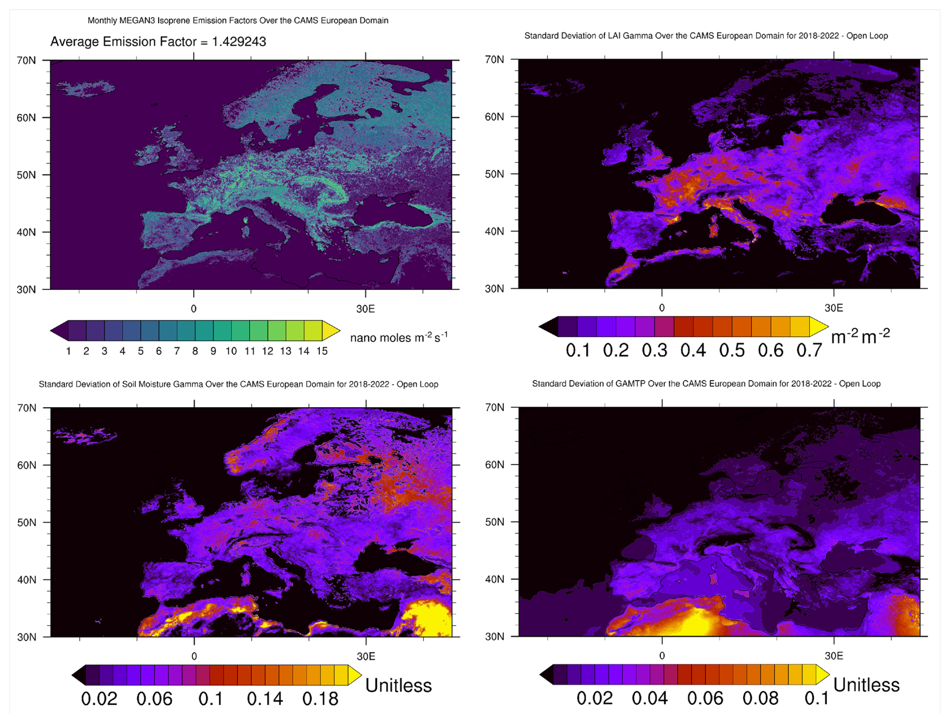
Figure 7 Maps of the MEGAN3.0 EFP isoprene emission factors in units of nmol m⁻² s⁻¹ (top left), the LAI gamma in units of m⁻² m⁻² (top right), the soil moisture gamma (unitless) (bottom left), and the temperature-radiation gamma in the bottom right.

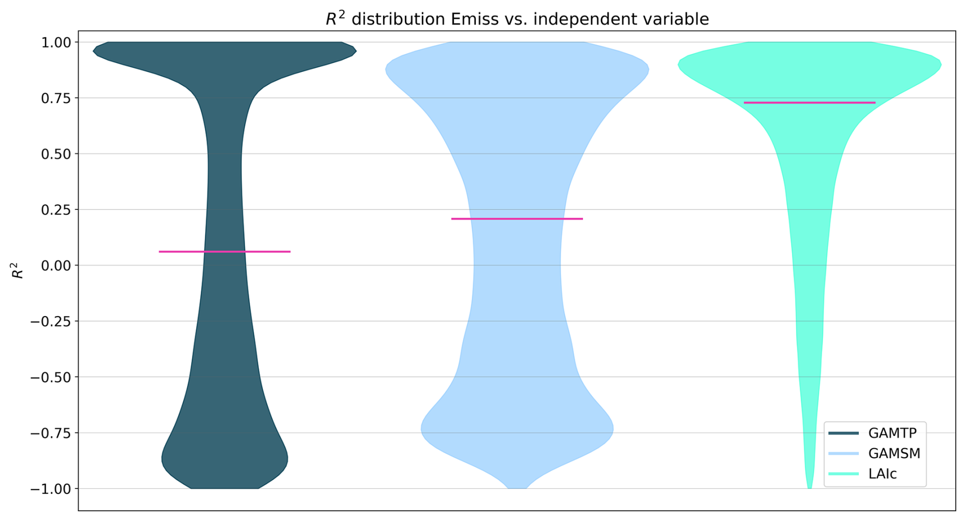
Figure 8 Violin plots showing the statistical distribution of R² correlation values between different activity parameters and the isoprene emissions calculated on a per grid cell basis averaged on an annual basis for each year from 2018–2022. The radiation-temperature gamma (GAMTP) is shown in dark green, the soil moisture gamma (GAMSM) in light blue, and LAI in turquoise. The pink horizontal bar in each plot represents the median R² value.

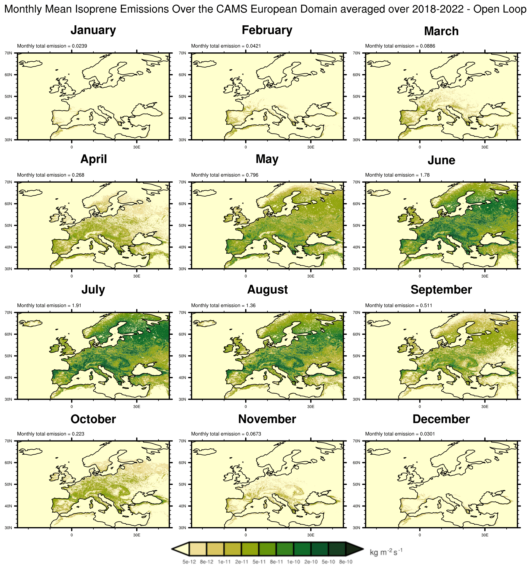
Figure 9 Maps of monthly mean isoprene emissions (units of kg m⁻² s⁻¹) calculated using the SURFEX-MEGAN3.0 algorithms and averaged over 2018–2022 using the open-loop configuration of SURFEX. The colour bars indicate increasing mean isoprene emissions as the colours transition from pale yellow to dark green. Note that the colour bar has a quasi-logarithmic scale. The monthly total mass of isoprene emissions (units of Tg) are shown above each plot.

We now examine the monthly and seasonal variability in the isoprene emissions. For this purpose, we present the monthly mean emissions from the OL-based dataset averaged over the 2018–2022 time period. This way we avoid presenting single years that can be affected by extremes in meteorology that lead to large increases or changes in isoprene emissions. For reference, however, the monthly means for all five years are presented in the Supplement (Figs. S9–13).

The monthly mean isoprene emissions over the CAMS European domain are shown in Fig. 9. First and foremost, we see the combined effects of the growing season, leading to changes in leaf area, and the annual cycle of sunlight and temperature during the year in this plot, with emissions at a minimum in the winter months and maximum in the summer months. Not only are the effects of the growing season visible from month to month, but we also see the progression of the growing season geographically. More southern regions have a growing season that starts earlier in the year compared to northern regions, but southern regions also show signs of reduced vegetation activity during summer as temperatures increase beyond optimal growing conditions. Similarly, western regions with milder maritime climates have increased emissions in the late winter and early spring compared to areas of eastern Europe with harsher continental-type winter conditions. Furthermore, the emissions peak in regions with higher densities of forest and thus emitting species and that coincide with regions with high levels of LAI (see Fig. 7).

There is a clear pattern presented in Fig. 10 showing how the different MEGAN activity parameters drive variability in the emissions over different timescales. According to Fig. 10a, the monthly variability in emissions is driven by variability in the radiation-temperature gamma and LAI, with radiation-temperature being the dominant of the two parameters influencing isoprene emissions. At the shorter timescales, i.e., daily and hourly shown in Fig. 10b and c, respectively, the radiation-temperature gamma increasingly dominates the variability in isoprene emissions compared to the other two parameters. Indeed, the correlation of the radiation-temperature gamma to emissions actually increases as the timescale shortens while the correlation of LAI to the emissions decreases markedly from monthly to hourly timescales. Figure 10 also shows that there is a remarkable consistency of the correlations of each parameter across each year that the dataset covers, i.e., 2018–2022. Indeed, there are only small variations in the median R² value across each year for each parameter and for each timescale. Furthermore, the shape of the distribution of the R² values for the radiation-temperature gamma is very consistent over all timescales and years. The R² values for LAI and the soil moisture gamma do differ, however, in this regard with each pairing of year and timescale displaying markedly different distribution from each other. The distribution of the R² of the soil moisture gamma varies widely, which is indicative of the varying influence this parameter has on controlling isoprene emissions.

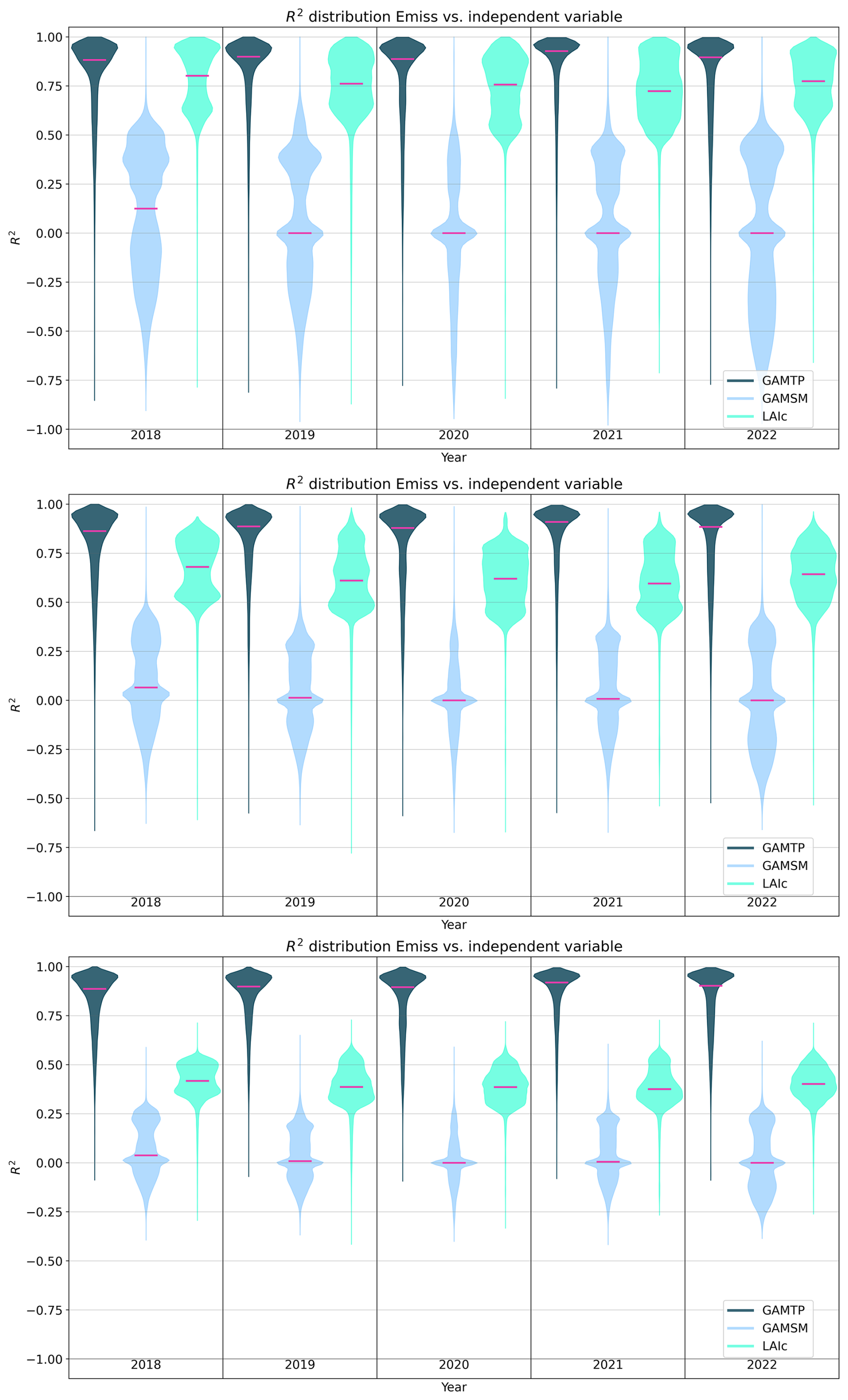
Figure 10 Violin plots showing the statistical distribution of R² correlation values between different activity parameters and the isoprene emissions calculated on a per grid cell basis over different averaging periods (monthly in plot (a), daily in plot (b), and hourly in plot (c)) for each year from 2018–2022. The radiation-temperature gamma (GAMTP) is shown in dark green, the soil moisture gamma (GAMSM) in light blue, and LAI in turquoise. The pink horizontal bar in each plot represents the median R² value.

We now examine the variability in the simulated isoprene emissions during the summer of 2019. We select data from 2019 to study and evaluate because 2019 presented some extreme and unseasonably hot conditions during the early summer that led to very large isoprene emissions. The results for the monthly mean isoprene emissions for the summer of 2019 are presented in Fig. 11 covering the June, July, and August period along with the monthly mean LAI from the SURFEX open-loop simulation. Later in the summer, hot, dry weather caused the vegetation phenology scheme within SURFEX to simulate strong reductions in leaf cover that led to reduced isoprene emissions. Indeed, isoprene emissions in 2019 peaked in June according to the SURFEX-MEGAN3.0 dataset, which makes 2019 unique among the five-year dataset since normally emissions peak in July within these data. Thus, 2019 presents an example of the impact extreme weather can have on isoprene emissions via its effect on vegetation represented by the vegetation phenology scheme. Visible within the maps, there are sharp declines in isoprene emissions within specific areas of Europe over this period, which can also be seen in the total emitted isoprene mass.

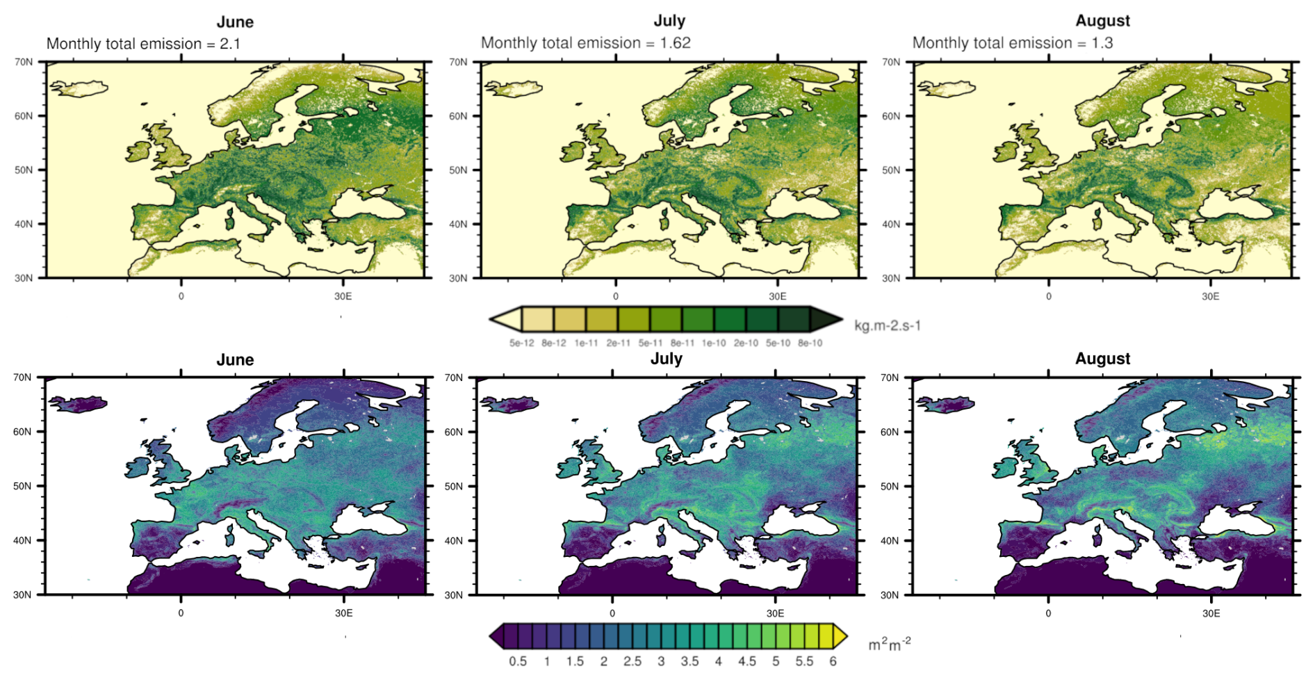
Figure 11 Maps of monthly mean isoprene emissions (units of kg m⁻² s⁻¹) calculated using the SURFEX-MEGAN3.0 algorithms using the LAI analysis configuration of SURFEX (top-row) and LAI (units m⁻² m⁻²) calculated by SURFEX in the open-loop configuration over the period June to August 2019. The panels sequentially show the monthly means for June, July, and August. The top row colour bars indicate increasing mean isoprene emissions as the colours transition from pale yellow to dark green. The bottom-row colour bars show increasing mean LAI as the colours transition from dark blue to yellow. The annual total mass of isoprene emissions (units of Tg) are shown above each plot in the top-row and the differences in annual total mass of isoprene emissions are shown above each plot in the top-row.

To further investigate this link, we plot the temporal correlations (on a daily-averaged timescale) of the isoprene emissions to LAI over this time period in Fig. 12. Figure 12a shows large areas of Europe with high correlation between LAI and the isoprene emissions, and it is possible to see that some of the areas with high correlation correspond to areas with large declines in LAI from June to August in Fig. 11. Furthermore, Fig. 12b shows the correlation between LAI and isoprene emissions only in areas where the LAI declined from June to August, and it is possible to see that the application of this mask to the dataset removed most of the areas with negative correlation between LAI and isoprene emissions. This evidence strongly suggests that the decline in LAI, which is driven by drought and heat stress on plants, is an important causative agent behind the reductions in isoprene emissions in the data during the summer of 2019. There are still some areas with negative correlation where the LAI declines yet isoprene emissions increase in Fig. 12b, e.g., in Portugal, and this is due to a strong increase in the radiation-temperature gamma variable over this region.

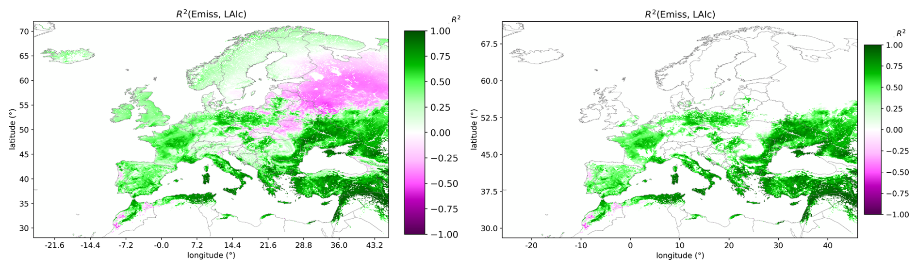
Figure 12 Maps of the correlation between LAI and the daily mean isoprene emissions over the CAMS European domain for the June to August 2019 time period. The left-hand panel shows the correlations for all grid cells within Europe while the right-hand panel shows the correlations only in locations where the LAI decreased between 1 June and 31 August. The colour bar shows green areas where the correlation was positive while the red areas shows where the correlation was negative.

This analysis proves that modelling the vegetation phenologically for MEGAN3.0 has a direct impact on the isoprene emissions it calculates during drought and heatwave conditions. This approach moves beyond using either a climatology or more simplistic phenological model to calculate LAI. Furthermore, since we have established the skill of the LAI simulation within prior discussions in Sect. 3.1, we can have some confidence that the representation of these changes in LAI and the consequent declines in isoprene are realistic.

3.2.2 Impact of LAI data assimilation

We next evaluate the impact that the LAI data assimilation step has on the estimation of isoprene emissions within the SURFEX-MEGAN3.0 system. The LAI assimilation analysis data from SURFEX is based on the data assimilation of LAI satellite observations. Suitable satellite observations were only available during the 2018–2020 period, so the evaluation of the use of the LAI analysis dataset only covers this 3-year period. Prior to analysing the effect of the LAI data assimilation step on isoprene emissions, we first evaluate the effect on LAI itself of performing the data assimilation step.

To evaluate the effect of the assimilation we plot in Fig. 13 the annual mean LAI analysis minus OL LAI difference for the three years (2018–2020) when we have coverage of both datasets. We can see that the LAI analysis is consistently higher than the OL over France, the UK, and Ireland and consistently lower over northern Italy, areas of the Iberian Peninsula, and eastern Europe. The absolute differences in LAI between the two datasets peak at around 0.4 m⁻² m⁻² over these highlighted regions and the absolute differences generally stay below 0.2 m⁻² m⁻². The difference between the analysis and OL calculated relative to the LAI analysis similarly shows peaks of ∼ 40 % (both positive and negative) over specific regions (e.g., regions of Spain, Italy, north Africa, and the Middle East) across the three years when these datasets are compared. Of the three years, 2019 is the year with the lowest relative differences and 2020 shows the largest relative differences.

We briefly discuss a further implication of this evaluation of the LAI data assimilation step. We can consider that the LAI assimilation step provides an indirect evaluation of the free-running model LAI from the OL simulation. This is because the LAI data assimilation step corrects the OL LAI simulation in regions where the OL model minus observations errors are large, which in turn leads to larger assimilation increments (either positive or negative) in these locations. Conversely, in areas where the increments are low, we can determine that the OL LAI estimates are already in closer agreement with the satellite observations of LAI.

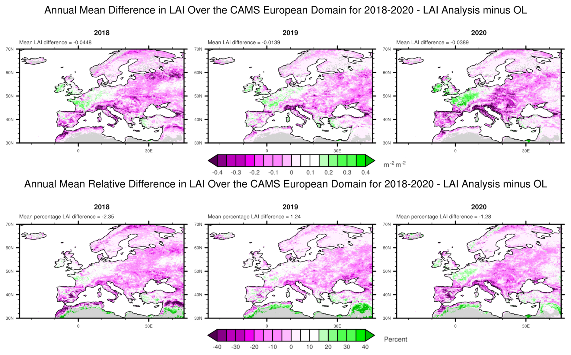
Figure 13 Maps of the absolute and relative difference in annual mean LAI (units of m⁻² m⁻²) between the LAI analysis minus the open-loop configurations over the period 2018–2020. The panels show each year over this time period moving sequentially from 2018 to 2022 from left to right. The colour bar indicates the difference in annual mean LAI between the LAI-analysis and open-loop configurations with red colours indicating larger annual mean open-loop LAI and green indicating larger LAI-analysis based LAI. The difference in annual mean LAI is shown above each plot.

Next, we analyse the impact that the LAI data assimilation has on the isoprene emissions both on an annual and monthly average basis. Our aim here is to directly evaluate the differences between the two emissions datasets (OL-based emissions and LAI-analysis based emissions) presented in this study. We first look at the annual averages and the results of this comparison are presented in Fig. 14. We have already presented the OL-based emissions in Sect. 3.2.1, so we only show the annual averages of the analysis-based emission data for 2018–2020 in Fig. 14 along with the analysis minus OL differences and the percentage difference in isoprene emissions between the two datasets. The annual average isoprene emission total calculated from the analysis-based emissions (calculated over 3 years 2018–2020) is 7.19 Tg yr⁻¹ with a standard deviation of 0.40 Tg yr⁻¹. Note that the average annual emitted isoprene from the OL-based emissions over this same time period were 7.14 Tg yr⁻¹ with a standard deviation of 0.44 Tg yr⁻¹. We identify three main findings from the analysis of these data. First, the impact of the data assimilation upon the overall annual emission totals is relatively small as we can see from the differences noted above the plots in the second row of Fig. 14. Second, while the impact on the sum of the emissions is minimal at continental scale (noting the annual average difference in emission totals), we see much stronger variations in the emissions within specific regions, e.g., the Iberian Peninsula in 2018, northern Italy, north Africa, and Croatia in 2020. Third, when we look at the percentage differences between the OL- and analysis-based datasets, we can see regions with large relative differences.

The impacts of the LAI assimilation on total and the monthly mean isoprene emissions appear modest for four reasons. First, the total isoprene emissions are subject to both temporal and spatial averaging, which leads to an effect whereby positive and negative assimilation increments cancel out over time and space leading to only small deviations from the open-loop. Second, the monthly mean emission maps are subject to temporal averaging that will over time lead to cancelling out of positive and negative LAI increments in time.

Beyond these purely statistical reasons, a third reason is that the underlying vegetation model in SURFEX, ISBA-a-gas, is quite skillful already at representing natural vegetation types when driven by good quality meteorological forcing and has been well validated in such cases (Delire et al., 2020). When the base model starts out with a good estimate of the observed state, this reduces the opportunity for the LAI assimilation step to make large improvements to the estimated state variable. Indeed, this effect was seen when using SURFEX to estimate soil moisture over the continental United States (Blyverket et al., 2019).

A fourth reason is that the ISBA-a-gs vegetation model is not a crop model and is designed to simulate natural vegetation types. It lacks the means to simulate cultivation processes such as ploughing, seeding, and harvesting, and only includes a prescriptive irrigation process. This means that the open-loop model typically has much larger errors in its representation of the true vegetation state. This means that the LAI assimilation offers an opportunity to correct LAI over regions with large proportions of crop cover. Indeed, this has been demonstrated in previous applications of the SURFEX model (see for example Albergel et al., 2017; Rojas-Munoz et al., 2023; and Jarlan et al., 2023 articles below). Furthermore, it should be noted that crops are not usually the largest source of isoprene. Thus, this may offer an explanation for why the impact on isoprene emissions of the assimilation step is limited.

A fifth reason is that the CANMET routine in MEGAN3.0 calculates the penetration of solar radiation through the vertical column of the canopy, and it can be considered that as LAI increases above 3 m⁻² m⁻² (see Fig. 11 for reference), solar radiation becomes significantly attenuated within the canopy. As such, increases in LAI beyond this threshold do not lead to large increases in isoprene emissions. This means that regions with lower levels of LAI (i.e., < 3 m⁻² m⁻²) are more sensitive to changes in LAI that result from the assimilation step. The effects of this are visible, for example, areas of the Iberian Peninsula and north Africa during 2018 and in northern Italy from 2018–2020.

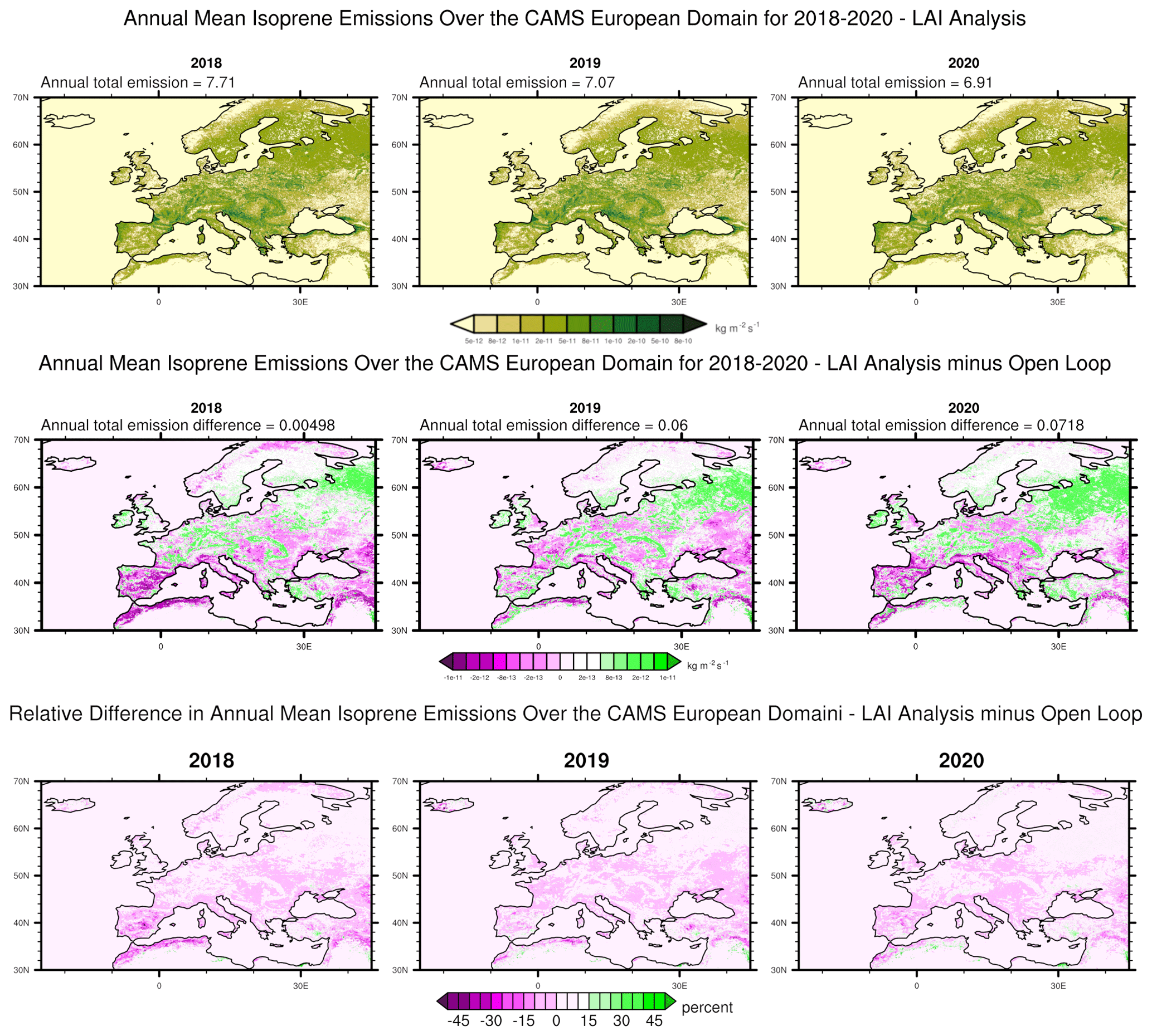
Figure 14 Maps of annual mean isoprene emissions (units of kg m⁻² s⁻¹) calculated using the SURFEX-MEGAN3.0 LAI analysis configuration of SURFEX (top-row), the difference between the LAI analysis minus the open-loop configurations (middle-row), and the percentage difference between the LAI analysis minus open-loop over the period 2018–2020. The panels show each year over this time period moving sequentially from 2018 to 2020 from left to right. The top-row colour bars indicate increasing mean isoprene emissions as the colours transition from pale yellow to dark green. The middle-row colour bars indicate the difference in annual mean isoprene emissions between the LAI-analysis and open-loop configurations with red colours indicating larger annual mean open-loop emissions and green indicating larger LAI-analysis based emissions. The bottom-row colour bar indicates the percentage difference in mean annual isoprene emissions between the LAI-analysis and open-loop with green indicating larger LAI-analysis based emissions and red indicating larger open-loop based emissions. The annual total mass of isoprene emissions (units of Tg) are shown above each plot in the top-row and the differences in annual total mass of isoprene emissions are shown above each plot in the middle-row.

We present the absolute monthly mean differences in analysis- and OL-based isoprene emissions averaged over the 2018–2020 time period in Fig. 15. When we analyse the impacts of the LAI assimilation on a monthly average basis, the absolute differences in isoprene emissions visible at regional scale resulting from the LAI data assimilation are larger than those seen in the annual averages (Fig. 14). Note that we have plotted the monthly mean analysis-based isoprene emissions averaged over 2018–2020 and these are shown in the Supplement (Figs. S14–S16). In addition, the monthly mean emissions for the assimilation analysis are also plotted for each year and shown in the Supplement (Fig. S17).

The magnitude of the absolute differences between the analysis- and OL-based emissions shown in Fig. 15 follows the growing cycle such that the size of the difference in emissions peaks when the emissions are at their highest for May through August. There are a few notable differences in emissions between the OL- and analysis-based emissions. First, the analysis-based emissions are larger in central and eastern Europe in April and May. Second, the picture becomes more complex in June, while Russia and the areas of higher altitude woodland across Europe (Carpathian mountains, Jura, Dinaric Alps, and Black Forest) show increased emissions in the analysis, areas of France, Turkey, the Iberian Peninsula, and north Africa show lower emissions compared to the OL. Lastly, in July and August, the OL emissions are larger than the analysis-based emissions over most of Europe, with France and Germany showing the largest differences between the two datasets.

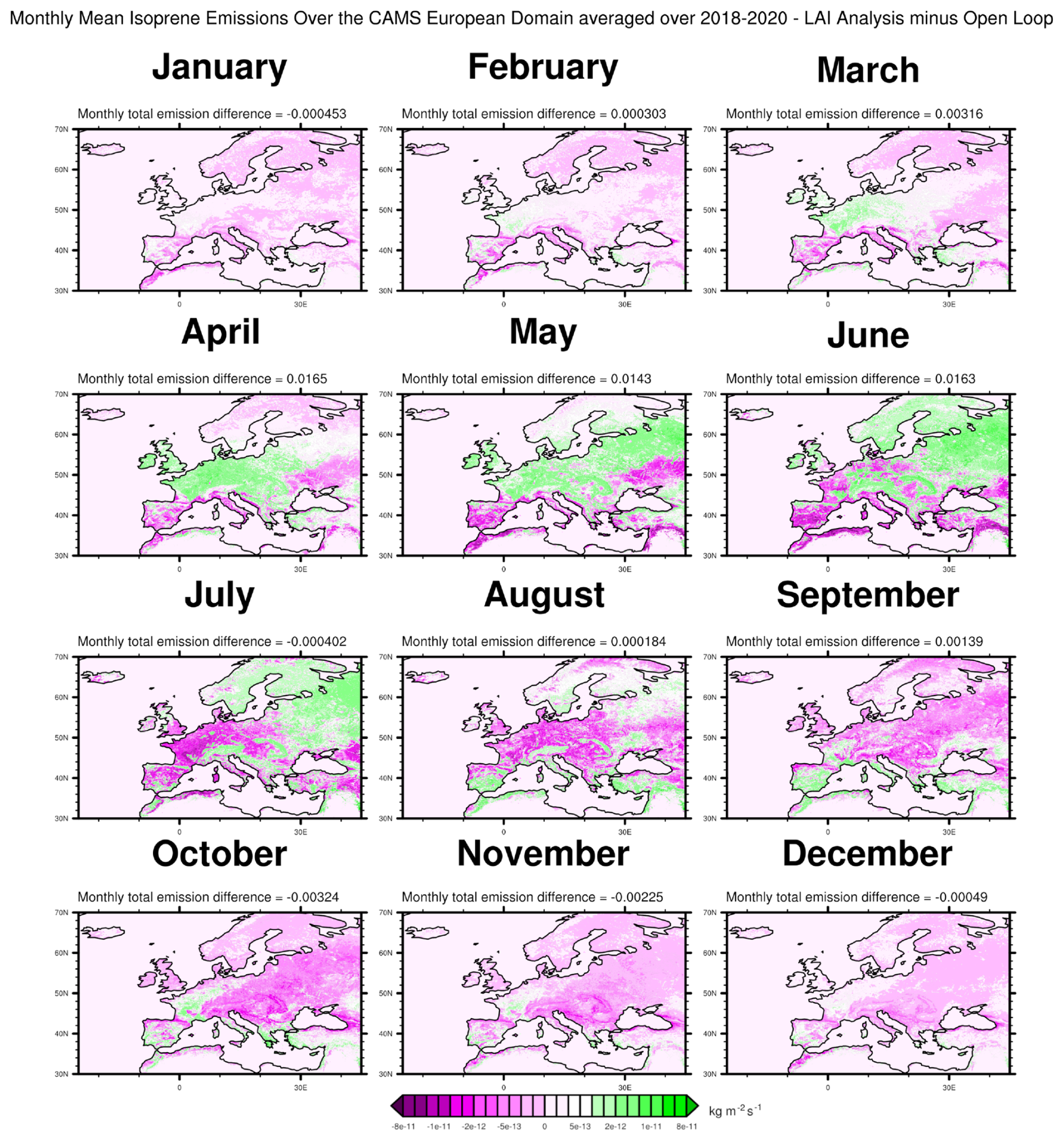
Figure 15 Maps of monthly mean (units of kg m⁻² s⁻¹) difference in isoprene emissions between the LAI analysis minus the open-loop configurations averaged over 2018 to 2020. The panels show each month during 2019 moving sequentially from January to December first from left to right and then from top to bottom. The colour bars indicate the difference in monthly mean isoprene emissions between the LAI-analysis and open-loop configurations with red colours indicating larger monthly mean open-loop emissions and green indicating larger LAI-analysis based emissions. The monthly total mass difference of isoprene emissions (units of Tg) are shown above each plot.

3.3 Comparison of SURFEX-MEGAN3.0 BVOC emissions with other datasets

We now perform an evaluation of the two BVOC emission datasets presented in this study. We perform this evaluation in two different ways. First, we evaluate the isoprene emission datasets against in-situ observations of isoprene from monitoring sites across Europe. And the second, we evaluate the isoprene emissions with respect to other emission datasets.

3.3.1 Evaluation using in-situ observations

We now evaluate the isoprene emissions using in-situ observations of isoprene concentrations obtained using the online gas-chromatograph (GC) technique. Note that we have excluded observations from other observation techniques, e.g., adsorption tube and canister sampling combined with the offline GC technique due to known issues involving systematic biases with observations obtained using these methods (Plass-Dülmer et al., 2006). In addition, these other observation techniques offer lower time resolution and sometimes do not provide continuous sampling. We have not included a comparison between our emissions and eddy covariance flux observations of isoprene. This is a limitation of this work that prevents an evaluation of the magnitude of the emissions and of the observed variability in emissions. One reason for this is that such observations are only available as part of short-term campaigns, which limits their usefulness for evaluating multiyear emission datasets.

The emissions are extracted for the geographical location of the in-situ observations for this comparison. Since we are not comparing like with like, we cannot perform a direct evaluation of the absolute values, and so we focus on performing an analysis of the temporal correlation between the emissions and ambient isoprene concentrations. To facilitate this comparison, we normalise the emissions and isoprene concentrations onto a common scale running from 0 to 1. This allows us to carry out an evaluation of the temporal variability of the emissions and to derive the temporal correlation in terms of R² between the simulated emissions and observations. We perform this analysis each year over the period 1 April though to 1 October. Although limiting the evaluation time period to the approximate duration of the growing season reduces the overall quality of the correlations leading to reduced R² scores, this mostly arises due to the removal of lower observed isoprene concentrations and emissions that occur during the wintertime. Including the lower values of both concentrations and emissions out of the growing season artificially boosts the scores. However, our objective here is to evaluate the higher temporal frequency of the day-to-day correlations. We also filter the data to remove all cases where the observations lay below the limit of detection (LOD). In addition, we remove data for particular years, for sites where there was either a lack of data, or there were apparent issues with the quality of the observations, i.e., large populations of data points near to the instrument LOD showing apparent systematic bias. The years we exclude are noted in relation to the compiled statistics shown in Table 4. Furthermore, we also excluded observations from very polluted urban sites in London, Paris, and Marseille due to concerns about contributions to ambient isoprene concentrations from anthropogenic sources (Khan et al., 2018).

We calculated the daily mean emissions from both emission datasets and daily mean isoprene concentrations at the location of each observation site. We then calculated the Pearson correlation coefficients between the emission-observation pairings for each year and site. We collate all the correlation coefficients for each site, and for each year of the dataset, and present them in Table 4.

Table 4 Correlation coefficients showing the correlation in time between daily mean isoprene emissions and daily mean isoprene concentrations calculated for a variety of monitoring sites across Europe. We calculate the correlation coefficients individually for each year for the OL (2018–2022 shown as O) and for the analysis (2018–2020 shown as A). The monitoring sites are distributed across France, the UK, Switzerland, Germany, and Finland. The stations Feyzin Stade, Vernaison, Eltham, Auchencorth, Beromünster, Zurich-Kaserne, Hohenpeissenberg, and Pallas are represented by the following three-letter acronyms, respectively, FEY, VER, ELT, AUC, BER, ZUR, HOH, and PAL. Station-year pairings marked with double crosses were removed due to lack of data or apparent data quality issues. Station-year pairings marked with dashes either lacked observations, emission data or both for that year.

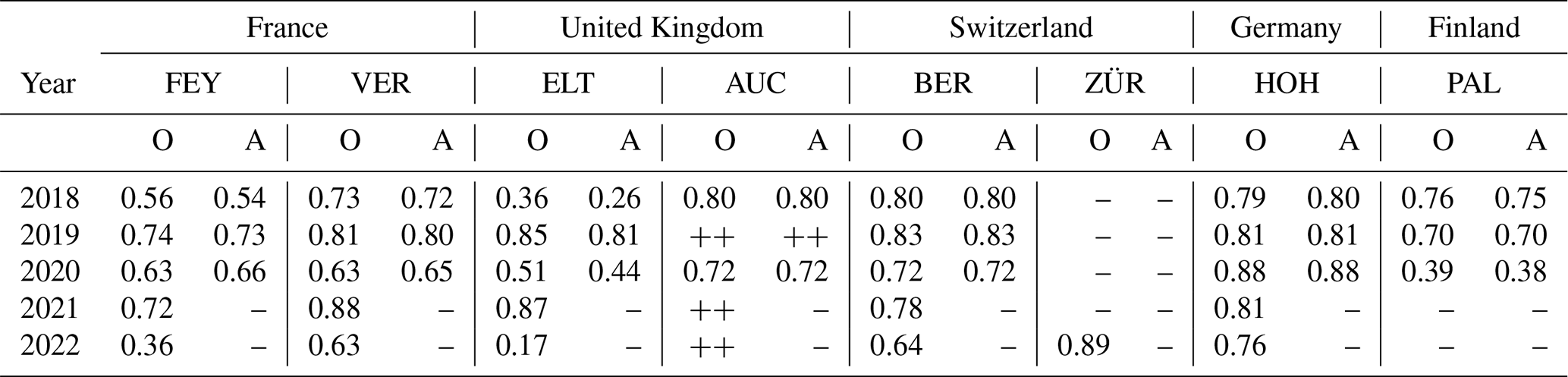
The correlations shown in Table 4 show that in general the isoprene emissions correlate with the observed isoprene concentrations at a moderate to strong level (22 cases of strong correlation > 0.7 R², 7 cases of moderate correlation > 0.4 R², and only 4 cases of weak correlation < 0.4 R²). The weakest correlations only occur at FEY in 2022, at ELT for 2018 and 2022, and at PAL in 2021. The ELT site is an urban background site located inside Greater London, so it is possible it is partially affected by anthropogenic sources of isoprene. In this case of the ELT, the poor correlations could be due to its proximity to London and therefore might experience influence from anthropogenic sources of isoprene (Khan et al., 2018). Note that the R² scores indicate there is no consistent improvement in the analysis emissions relative to the open-loop emissions. There are instances (both specific years and locations) where the analysis has both higher and lower correlation than the open-loop but overall there is not a strong indication either way which has consistently better correlation. This is in spite of the fact that the LAI analysis shows higher correlation with the independent TROPOMI SIF observations than the open-loop (see Sect. 3.1).

The SURFEX-MEGAN3.0 open-loop emissions were evaluated in a recent study detailing a Europe-wide 1-week measurement campaign focused on VOCs (Aas et al., 2025). This evaluation showed that the SURFEX-MEGAN3.0 open-loop emissions correlated well with observed isoprene concentrations at roughly half of the sites included in the study, albeit for a short time period.

Overall, this evaluation shows that the two isoprene emission datasets are able to capture the temporal variability of emissions on daily timescales. This is encouraging given that this comparison compares emissions to concentrations and there are several likely sources of error that would obfuscate such a comparison. First, there is the issue of the representativity of the 0.1° × 0.1° grid scale to the observation sites, which is important because of isoprene's very short lifetime. Second, isoprene's ambient concentration can also be affected by the abundance of its sinks, the hydroxyl radical, the nitrate radical, and ozone, which are ignored when only looking at the emissions. Lastly, other meteorological effects such as wind, turbulence, and boundary layer height are implicitly ignored in this comparison. For instance, higher wind speeds and/or boundary layer heights would lead to lower ambient isoprene concentrations for the same emission source strength. The weak to moderate correlations found at some sites and for some years imply that further study is required to further understand and interpret the potential sources of model error underpinning the poor performance of our datasets in these cases.

3.3.2 Evaluation using other emission datasets

A primary motivation of this work was to develop two BVOC datasets that could be used to support the study of European air quality specifically in relation to CAMS. We therefore perform an evaluation of the SURFEX-MEGAN3.0 emission datasets by comparing them to the MEGAN-MACC (Sindelarova et al., 2014) and CAMS-GLOB-BIO (Sindelarova et al., 2022) BVOC emission datasets that were developed within the frame of CAMS. Furthermore, these datasets have received recent attention and represent the current state of the art in terms of emission modelling for Europe using MEGAN. In the case of the CAMS-GLOB-BIO emissions, we include a comparison with the v1.2, v3.0, and v3.1 versions of this dataset.

A timeseries of the monthly mean isoprene emissions for each of these datasets is calculated over the CAMS European domain and plotted in Fig. 16. In addition, in Table 5, we present a compilation of the annual emission totals for isoprene for each dataset and each year they are available. According to these comparisons, the MEGAN-MACC emission inventory is the dataset with the highest overall emissions over the period 2018–2020 over the CAMS domain. Meanwhile, the two SURFEX-MEGAN3.0 emission datasets are very similar to one another, and it is possible to see only minor differences during the periods with the highest isoprene emissions in the summertime. The SURFEX-MEGAN3.0 datasets are also very similar to the CAMS-GLOB-BIOv1.2 dataset, which appears to be coincidental given the large difference in input data and MEGAN model version used (i.e., version 2.1 in the case of CAMS-GLOB-BIOv1.2). On the other hand, both the CAMS-GLOB-BIOv3.0 and CAMS-GLOB-BIOv3.1 dataset emissions are both lower overall compared to the SURFEX-MEGAN3.0 datasets.

Aside from differences in the absolute magnitude of the emissions, Fig. 16 shows that the different datasets also have different seasonalities from each other. The SURFEX-MEGAN3.0 and the CAMS-GLOB-BIOv3.1 represent the two most contrasting emission datasets in terms of seasonality. Out of all of the emission datasets, the SURFEX-MEGAN3.0 emissions consistently peaks earliest in the summer season (i.e., June to July) while the CAMS-GLOB-BIOv3.1 always peak the latest in the summer season (i.e., July to August).

We only have this comparison for the 2018–2019 period for v3.0, and the 2018–July 2019 period for v1.2, but both of these two CAMS-GLOB-BIO datasets show a similar month-to-month variability to that of the SURFEX-MEGAN3.0 datasets, i.e., peaks in emissions towards the early part of summer on average. Although both datasets do show a more prolonged peak lasting into July in 2019. Meanwhile, the MEGAN-MACC emissions show their highest peak in emissions in June during 2018 and during July during 2019 and 2020 placing it overall somewhat between the SURFEX-MEGAN3.0 and CAMS-GLOB_BIOv3.1 emissions.

We have evaluated the underlying causes of the differences in seasonality and magnitude highlighted between the different emission datasets. This evaluation included analysing the different meteorological datasets and their effects on the radiation-temperature gamma variable (influenced by temperature and solar radiation), LAI, and the effect of soil moisture upon the SURFEX-MEGAN3.0 emissions (note that the other isoprene emissions in this example do not consider soil moisture effects). This evaluation revealed several findings. The differences in the meteorology used in SURFEX-MEGAN3.0 (HRES) and CAMS-GLOB-BIOv3.0/3.1 (ERA5) were likely only a very minor factor in explaining the differences between these emission inventories. We directly compared the radiation-temperature gamma values from SURFEX-MEGAN3.0 and CAMS-GLOB-BIOv3.1 (identical to v3.0) in Fig. S18 of the Supplement. This comparison shows that the only significant differences in radiation-temperature gamma occurred in desert regions (e.g., north Africa and the Middle East) year round and in southern Mediterranean regions during summer when vegetation cover is very low and the emissions from these regions are relatively minor. With regards to the comparison between SURFEX-MEGAN3.0 and MEGAN-MACC, Sindelarova et al. (2022) found that the MERRA/MERRA-2 meteorological forcing (used to make MEGAN-MACC) had higher 2-meter temperature and PAR values than the ERA5 data (used in CAMS-GLOB-BIOv3-0/3.1) and that this explained why the MEGAN-MACC inventory had much higher isoprene emissions. We can apply that same finding here to conclude that the MEGAN-MACC emissions are much higher than the SURFEX-MEGAN3.0 emissions due to the different meteorological parameters of MERRA/MERRA-2. This is further supported by the good consistency of the radiation-temperature gamma values derived from HRES and ERA5 shown in Fig. S18.

Evaluating LAI, we found that in general the LAI dataset (based on Yuan et al., 2011) used to calculate the monthly emission factors in the CAMS-GLOB-BIOv3.1 emissions tends to peak later in the summer than the LAI calculated by SURFEX. The CAMS-GLOB-BIOv3.1 emissions used this same monthly climatological mean of LAI (averaged over 2007–2016) derived from MODIS (Sindelarova et al., 2022; Yuan et al., 2011) to calculate the LAI used for the MEGAN activity factor calculations after 2016. As a result, in years where SURFEX estimated particularly extreme deviations in LAI from the historical climatology with an early peak in LAI, e.g., 2019, the divergent effect on the emission seasonality is even greater. The monthly mean LAI analysis data from SURFEX for 2019 are presented in Fig. S19 of the Supplement along with the LAI 2007–2016 climatological monthly means used in CAMS-GLOB-BIOv3.1 (Fig. S20) for the purposes of demonstrating this point. Indeed, it is possible to see large reductions in the monthly mean LAI data from June into July and August during 2019 in the SURFEX LAI data in important isoprene emitting regions (see Fig. S15 showing the monthly mean isoprene in 2019 for reference) that are not visible in the corresponding panels of Fig. S20. In terms of the overall magnitude, the annual mean of the SURFEX assimilation analysis LAI over the European domain was 1.12, 1.15, and 1.18 m⁻² m⁻² in the years 2018, 2019, and 2020, respectively, compared to the mean of the climatological LAI of 1.00 m⁻² m⁻² from Yuan et al. (2011) used by CAMS-GLOB-BIOv3.1. The annual mean LAIs from the OL for 2021 and 2022 were 1.24 and 1.17 m⁻² m⁻², respectively. Thus, this indicates that the magnitude of the SURFEX LAI is slightly higher than that used by CAMS-GLOB-BIOv3.1. Lastly, validation of the CLMS LAI product from PROBA-V (Sanchez-Zapero et al., 2018) indicates that the that the MODIS LAI product has much higher uncertainty. Thus, one interpretation is that the larger systematic uncertainties in the MODIS LAI product drive some of these differences.

The emission factors used in the different emission inventories contribute another important source of uncertainty and likely also play an additional role in explaining the differences in their magnitude. It is well established that uncertainties in emission factors are in important contributor to the overall uncertainty in emissions (Keenan et al., 2009; Oderbolz et al., 2013; Rinne et al., 2009; Simpson et al., 1999). Sindelarova et al. (2022) found that changing from the MEGANv2.1 to the EMEP emission factors, respectively, accounted for the higher estimated emissions over Europe of CAMS-GLOB-BIOv3.0 compared to CAMS-GLOB-BIOv3.1.

We compare the emission factors in this study (see Fig. 7) to the emission factors for the CAMS-GLOB-BIOv3.0 and v3.1 emission inventories (Sindelarova et al., 2022) over Europe (see the Supplement with CAMS-GLOB-BIOv3.0 in Fig. S21 and CAMS-GLOB-BIOv3.1 in Fig. S22). Due to differences in approach, it is not possible to compare the absolute magnitude of the emission factors shown in Fig. 7 compared to those in Figs. S21 and S22. This is because a different set of standard conditions were used by CAMS-GLOB-BIO from those used by SURFEX-MEGAN3.0. Furthermore, CAMS-GLOB-BIO, which is built on MEGAN2.1, uses a canopy-level approach instead of the leaf-level approach used in SURFEX-MEGAN3.0. Thus, the CAMS-GLOB-BIO emission factors include a multiplication by a standard LAI value of 5 m⁻² m⁻² for 3.0 and by a monthly climatological LAI derived from (Yuan et al., 2011) for 3.1, whereas LAI is only treated within the activity factor calculations in SURFEX-MEGAN3.0.

Comparing Figs. 7, S21, and S22, we determine that the SURFEX-MEGAN3.0/MEGAN EFP emission factors are more similar in their spatial distribution to those from CAMS-GLOB-BIOv3.0/MEGANv2.1 than the CAMS-GLOB-BIOv3.1/EMEP-based emission factors. The spatial patterns of the EMEP-based emission factors show much more heterogeneity than the MEGAN3.0 emission factors and show both maxima and minima in different regions. The EMEP-based emission factors show specific regions that have much higher relative values associated with broadleaf species in southern Europe on the one hand and areas that have relatively much lower values in central Europe and mountainous regions on the other. The MEGAN2.1 emission factors used in CAMS-GLOB-BIOv3.0 are more spatially smooth with less heterogeneity, which is a point of similarity with SURFEX-MEGAN3.0. The MEGAN2.1 emission factors do show peak values similar regions, e.g., mountainous regions like the Pyrenees, Alps, Balkans, and Carpathians, but differ by showing peaks in Russia, northern Norway, and Galicia.

(Sindelarova et al., 2022) determined that the increased heterogeneity of the EMEP-based emission factors, particularly the large regions in Europe with relatively low values, contributed to the lower emissions that they calculated for CAMS-GLOB-BIOv3.1 compared to CAMS-GLOB-BIOv3.0. Following the same logic, and given the differences we see comparing SURFEX-MEGAN3.0 to the more heterogeneous EMEP-based emission factors, we attribute the higher SURFEX-MEGAN3.0 emissions compared to the CAMS-GLOB-BIOv3.1 emissions to be largely due to the effect of the emission factors.

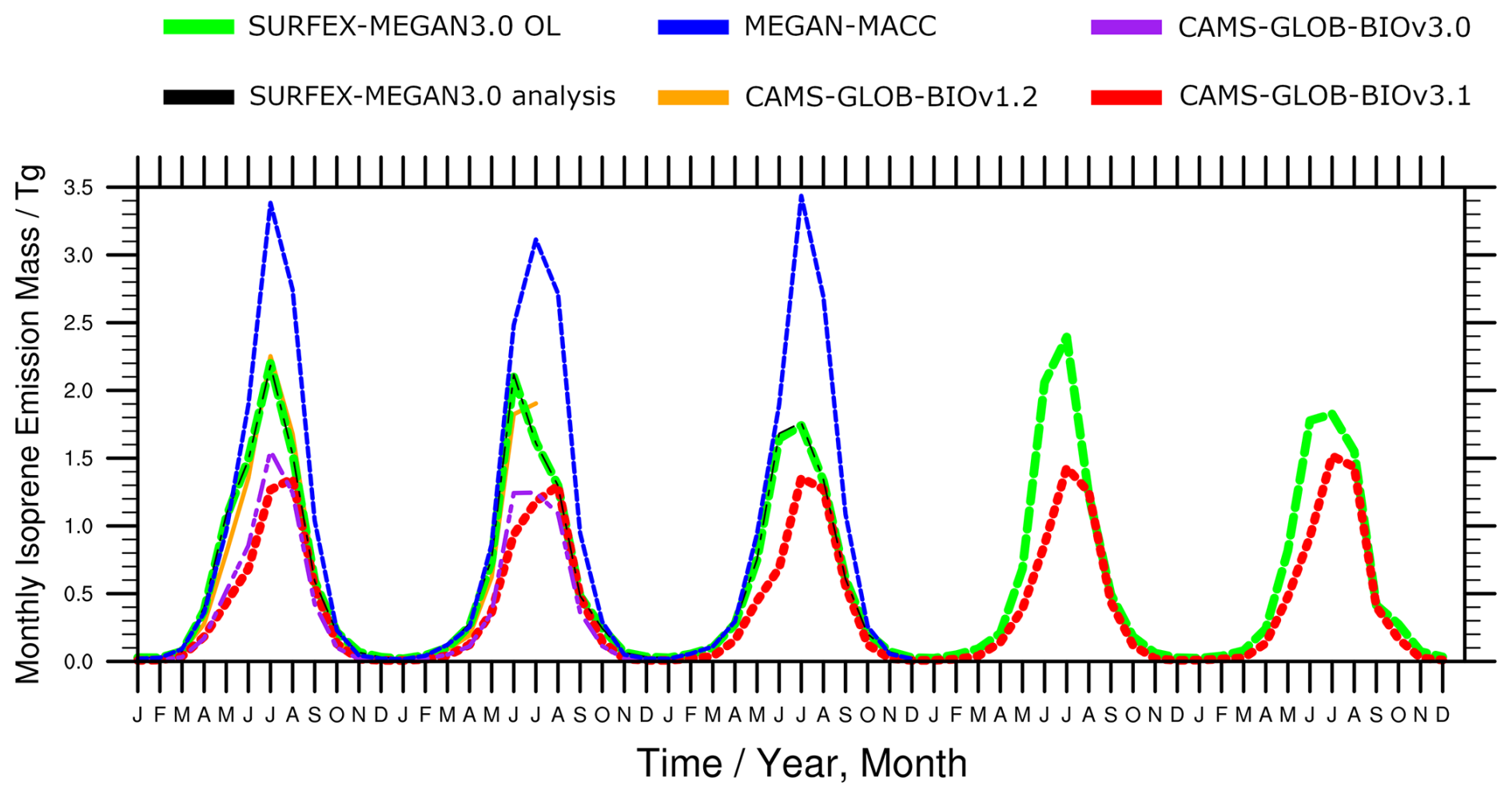
Figure 16 A time series of the monthly mean total emitted isoprene over the 2018–2022 period as calculated the SURFEX-MEGAN3.0 OL (green solid), SURFEX-MEGAN3.0 analysis (black dot-dash), MEGAN-MACC (blue dash), CAMS-GLOB-BIOv1.2 (orange solid), CAMS-GLOB-BIOv3.0 (purple dash), and CAMS-GLOB-BIOv3.1 (red dash), emission inventories. The units of the isoprene emission totals are in Tg. The SURFEX-MEGAN3.0 OL and CAMS-GLOB-BIOv3.1 emission inventories are available over the full time period of 2018–2022, while the SURFEX-MEGAN3.0 analysis and MEGAN-MACC emissions are only available over the period 2018–2020, the CAMS-GLOB-BIOv1.2 are only available 2018–July 2019, and the CAMS-GLOB-BIOv3.0 are only available 2018–2019.

Overall, this evaluation shows that the magnitude of the total isoprene emissions within the CAMS European domain of SURFEX-MEGAN3.0 emissions falls well within the bounds set by existing isoprene emission inventories. Indeed, both datasets fall within the upper and lower bounds set by the most recent published isoprene emission datasets published in association with the MACC and CAMS projects. There are some notable differences from other datasets in terms of the seasonal variability. Further study and evaluation will be required to determine if this difference represents a realistic seasonal variability. The evaluation performed in Sect. 3.3.1 provides some support for the variability represented in both the OL and analysis-based datasets.

We quickly discuss the magnitude of the global isoprene emissions from the MEGAN-MACC and CAMS-GLOB-BIO datasets. In the case of MEGAN-MACC, the global BVOC emissions were estimated to be 760 Tg (C) yr⁻¹ with 70 % of this carbon mass from isoprene (602.9 Tg (isoprene) yr⁻¹) over the 30-year period from 1980 to 2010 that was studied. In the case of CAMS-GLOB-BIO four estimates were made ranging between 424 and 591 Tg (C) yr⁻¹ (299.1 to 440.5 Tg (isoprene) yr⁻¹), with CAMS-GLOB-BIOv3.1 being the recommended data set according to the authors (591 Tg (C) yr⁻¹ and 440.5 Tg (isoprene) yr⁻¹). Overall, the emission totals calculated over the CAMS European domain and presented in Table 5 represent only a small fraction of the global emission totals.

Table 5 Annual total emitted isoprene in Tg over the CAMS European modelling domain as determined by the SURFEX-MEGAN3.0 OL, SURFEX-MEGAN3.0 analysis, and CAMS-GLOB-BIOv3.1 emission inventories. The emission datasets are available over different time periods. The SURFEX-MEGAN3.0 OL and CAMS-GLOB-BIOv3.1 emission inventories are available over the full tie period of 2018–2022, while the SURFEX-MEGAN3.0 analysis emissions are only available over the period 2018–2020. These annual emission totals are calculated from 1 January to 31 December in all cases except for CAMS-GLOB-BIOv1.2 that for 2019 were calculated January through to July.

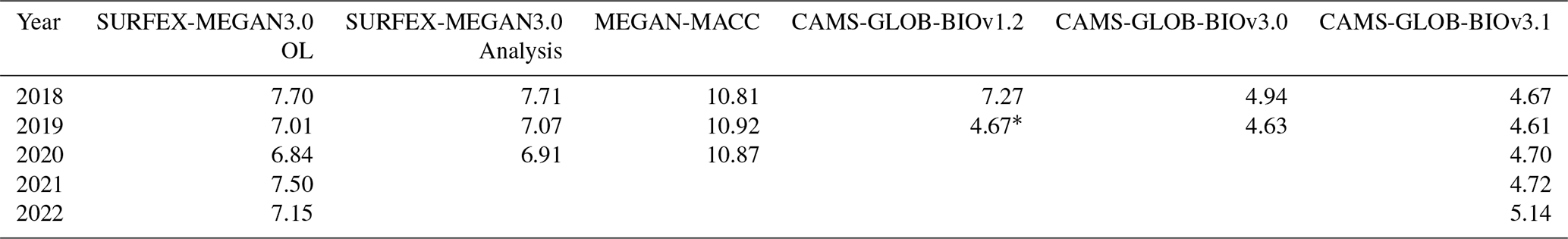
^∗ Only calculated over January through to July 2019

4 Data availability

Both of the isoprene emission datasets are available as hourly means at a spatial resolution of 0.1° × 0.1° over the CAMS European domain. The data can be accessed from the SEEDS project data portal (https://www.seedsproject.eu/data, last access: 17 July 2025) and are available in Zarr format or can alternatively be downloaded in netcdf format using a short python script by following the instructions provided. The other compounds (including isoprene again) are available on the Harvard Dataverse inside the dataverse for the SEEDS project (https://dataverse.harvard.edu/dataverse/Horizon-SEEDS-project, last access: 17 July 2025). Two different datasets were created within the SEEDS dataverse, one each for the analysis (https://doi.org/10.7910/DVN/LAUVTU, Hamer et al., 2025a) and OL (https://doi.org/10.7910/DVN/69G1FX, Hamer et al., 2025b).

5 Conclusions

We have presented two new datasets of BVOC emission inventories that cover the CAMS European domain that are both publicly available and ready for use in applications related to the study of European scale air quality. As per this intention, both datasets were produced at a spatial resolution of 0.1° × 0.1° exactly matching the spatial domain utilised by the CAMS European regional forecast and analyses. The datasets were produced within the framework of the EU's SEEDS project and are called SURFEX-MEGAN3.0 OL and SURFEX-MEGAN3.0 analysis. The OL dataset is available over a five-year period from 2018–2022 and the analysis dataset is available over the three-year period 2018–2020.

Another motivation for the production of this new dataset was to address key uncertainties in BVOC emission modelling arising from representation of vegetation phenology and to move towards an Earth-systems approach allowing feedbacks and interactions between meteorology/climate, vegetation, and atmospheric composition. To this end, we applied a methodology based on using a land surface model capable of vegetation phenological modelling that responds to an externally applied meteorological forcing. To further address uncertainties in the simulation of vegetation phenology, the land surface model is further supported by data assimilation of satellite observations of LAI to create an assimilation analysis, which forms the basis of the analysis emission dataset. In addition, we also used the most recent version (at the beginning of the study) of MEGAN3.0.

Since we used SURFEX land surface model within the MEGAN3.0 production chain, we perform an evaluation of the key variables estimated by SURFEX that are used within MEGAN3.0. We evaluated both LAI and RZSM. In the case of LAI, we use observations of SIF from the TROPOMI satellite to establish that the SURFEX LAI datasets have good skill over the main body of Europe, the UK, Italy, Ireland, southern Sweden and into eastern Europe as well and that the analysis for LAI had improved correlation to SIF compared to the OL. The RZSM was evaluated against in-situ observations in south-western France and was shown to have strong year-round correlation and moderate correlation during the summertime. The RZSM analysis performed better than the RZSM OL.

Analysis of the OL emission dataset over the 5-year period 2018–2022 shows that the average annual isoprene emissions were 7.20 Tg yr⁻¹ and had a standard deviation of 0.28 Tg yr⁻¹. The difference between the year with the largest (2018) and smallest (2020) emissions was equivalent to 11.4 % of the average annual emission. The analysis-based average (calculated over 3 years 2018–2020) is 7.19 Tg yr⁻¹ with a standard deviation of 0.40 Tg yr⁻¹. Note that the average of the OL-based emissions over this same time period was 7.14 Tg yr⁻¹ with a standard deviation of 0.44 Tg yr⁻¹. The areas with the highest inter-annual variability correspond to areas of large standing woodland with the densest levels of emitting plant species. Analysis showed that this variability is induced by (listed with decreasing importance) variability in LAI, meteorology (temperature and radiation), and RZSM. LAI had the consistently highest correlation with isoprene emissions on the inter-annual timescale indicating the important role that variations in vegetation and any induced effects by meteorology (e.g., affecting the growing season and drought) can play.

Analysis of the monthly variations in the OL dataset averaged over the 5-year period 2018–2022 show that monthly isoprene emissions follow the development of the growing season within different climatic zones. Isoprene emissions peak during the summer period (June through August) and are highest on average in July. An analysis of the underlying factors (listed in decreasing importance) driving the monthly variability showed that meteorology (temperature and radiation), LAI, and RSZM impacted the changes in isoprene emissions. This finding was reproduced consistently for all five years in the OL dataset. The importance of situations where extreme meteorological conditions can impact vegetation were highlighted in the context of the summer of 2019. Here, it was shown that reductions in LAI driven by extreme heat and drought led to decreased isoprene emissions in the month of July compared to June of that same year.

The evaluations and analysis performed on these datasets at annual and monthly timescales highlights the importance of including a representation of vegetation phenology by using a land surface model in the MEGAN emission production chain. Furthermore, this highlights the potential advantages of an Earth system approach to BVOC emission modelling.

Performing the LAI data assimilation step does not impact the average annual LAI levels or the total magnitude of isoprene emissions at the continental scale to a significant degree either on monthly or annual timescales. However, larger absolute and relative variations in emissions and LAI do occur when looking at smaller spatial scales. The impact of the LAI data assimilation step is largest during the summertime.

We evaluate the temporal (daily) correlation of isoprene emissions with in-situ observations of isoprene concentrations from 8 sites across Europe. We find that both the OL and analysis datasets have moderate (> 0.4 R²) to strong (> 0.7 R²) temporal correlation with the in-situ observations for the majority of years and sites analysed with only 4 cases (site-year parings) showing weak (< 0.4 R²) correlation. This indicates that, overall, this method has good skill at estimating the temporal variability in the emissions. No overall strong difference between the skill of the OL and analysis datasets was found when the emissions were evaluated in this manner using in-situ observations.

Compared to other isoprene emission datasets produced within the frame of MACC and CAMS, the two SURFEX-MEGAN3.0 datasets estimate emission totals lie between the minimum (CAMS-GLOB-BIOv3.1) and maximum (MEGAN-MACC) estimates in isoprene emissions over the CAMS European domain for the 2018–2020 time period. Indeed, the SURFEX-MEGAN3.0 isoprene emissions were very similar in magnitude to the CAMS-GLOB-BIOv1.2 isoprene emissions. Part of the difference in the absolute magnitude in the SURFEX-MEGAN3.0 and CAMS-GLOB-BIOv3.1 emissions was attributed to the difference in emission factors used to calculate both emission inventories. With the SURFEX-MEGAN3.0 emission factors generally having an effect that increased the isoprene emissions relative to those from CAMS-GLOB-BIOv3.1. This highlights the need for more study on emission factors in Europe and for us to update the emission factors in future work related to specific emitting vegetation species. Work to evaluate and improve the European emission factors in both EMEP and CAMS-GLOB-BIO is underway in other EU projects (CAMAERA, https://camaera-project.eu/, last access: 6 February 2026 and the continuation of CAMS2-61, Denier van der Gon et al., 2025), and any improvements can be incorporated in future applications of SURFEX-MEGAN3.0.

We did also note large differences in the seasonality of the different datasets whereby the SURFEX-MEGAN3.0, CAMS-GLOB-BIOv1.2, and CAMS-GLOB-BIOv3.0 emissions peaked earlier in summer, the MEGAN-MACC emissions peaked in the middle of summer, and the CAMS-GLOB-BIOv3.1 emissions peaked the latest in summer. An investigation showed that the differences between the earliest (SURFEX-MEGAN3.0) and latest peaking emissions (CAMS-GLOB-BIOv3.1) were due to differences in the seasonality of the LAI datasets used in the two different approaches whereby the LAI estimated by the SURFEX OL and analysis tended to peak earlier than the MODIS based LAI used for CAMS-GLOB-BIOv3.1 (Sindelarova et al., 2022; Yuan et al., 2011). These differences lead to substantial differences between these two emission datasets when compared on a month-by-month basis like this and it highlights the importance of our approach attempting to improve the temporal variability of LAI datasets used in the MEGAN algorithm. Indeed, Guenther et al., 2006 identify that uncertainties in LAI input data could impact global, annual isoprene emissions from −11 % to 29 %, but we see much larger relative differences between the SURFEX-MEGAN3.0 and CAMS-GLOB-BIOv3.1 emissions over Europe when compared on a month-to-month basis. Future work aimed at further intercomparisons of LAI input datasets would be valuable to support further advancement on this topic.

We now address the various limitations of our work. First, we did not include a comparison with flux tower measurements nor did we test our emissions in an atmospheric model to simulate atmospheric concentrations of isoprene and secondary chemical species. Both would be valuable ways to extend our work in the future. There were also a series of methodological choices that affected the uncertainties of the presented emissions that could be addressed via sensitivity tests and form the basis of future work. For instance, we only used a single set of emission factors to calculate the emissions, and given their associated uncertainties, it would be worthwhile to investigate this further and test other emission factors in the future. We used the grid-averaged LAI output from SURFEX, but it would be worthwhile to test using the PFT-specific LAI values and then calculate the emissions separately for each PFT within each grid cell, e.g., following the approach of Oumami et al. (2024). Lastly, it would be worthwhile to test the trade-off of using coarser resolution meteorological reanalysis versus higher resolution meteorological forecast. We evaluated that the latter would be advantageous when designing this study but testing the former would help to evaluate that hypothesis further.

Guenther et al. (2006) and Sindelarova et al. (2022) point to other sources of uncertainty that we do not directly address in this work, which include mapping and consistency of plant functional types (PFTs) and the manner in which the impacts of soil moisture and drought are treated within the MEGAN algorithm. Addressing these uncertainties in future work will be a priority in order to further improve the quality of emissions produced using the SURFEX-MEGAN3.0 algorithm. Indeed, the work of Oumami et al. (2024) already highlights the advantage of harmonizing PFTs between SURFEX and MEGAN, so it would be advantageous to use the SURFEX PFTs derived from either ECOCLIMAP-II (Faroux et al., 2013) or ECOCLIMAP-SG (Druel et al., 2022) as a basis for calculating the EFs used by MEGAN in the future. One further limitation of our work was the inconsistency between the land use datasets used in the SURFEX land surface model and the MEGAN EFP tool for calculating emission factors. This inconsistency should be corrected in future work following the example of Oumami et al. (2024) and Sindelarova et al. (2022).

Accurately representing the impacts of soil moisture and drought on BVOC emissions is another important area of research. In light of the large uncertainties of the role of soil moisture and drought, some groups (Oomen et al., 2024; Sindelarova et al., 2022) have taken an approach to exclude the influence of soil moisture in the MEGAN algorithm. There is compelling evidence (Bonn et al., 2019; Jiang et al., 2018; Pegoraro et al., 2004; Yuan et al., 2016; Zheng et al., 2017), however, that vegetation response to soil moisture and drought plays an important role in BVOC emission variability, and this remains an open research question of how this should be addressed in a generalized way within the MEGAN model framework. The newly proposed parametrization of soil moisture stress on isoprene described in (Wang et al., 2022) was tested in CAMS-GLOB-BIO and led to a decrease in global isoprene total emissions by 15 %, with even larger reductions in dry regions such as Australia, sub-Saharan Africa or Middle East (K. Sindelarova, personal communication, 2025). Future work should therefore address this source of uncertainty by testing different algorithms for different drought situations for varied climatic zones and ecotypes.