GEOXYGEN: a global long-term dissolved oxygen dataset based on biogeochemistry-aware machine learning framework and multi-source observations

Dissolved oxygen (DO) serves as an essential indicator of marine ecosystem health. However, sparse and uneven observations have limited our ability to characterize its full spatiotemporal variability, underscoring the continued need for long-term, high-resolution, and physically consistent global DO datasets. Here, we present GEOXYGEN, a global dataset of monthly DO fields at 0.5° × 0.5° resolution spanning 1960–2024 and depths from the surface to 5500 m (Wang et al., 2026a, https://doi.org/10.5281/zenodo.19703198; Wang et al., 2026b, https://doi.org/10.12157/IOCAS.20260223.002). GEOXYGEN is generated with a hierarchical modeling framework that accounts for regional and vertical heterogeneity. By combining physical and biogeochemical predictors with an adaptive feature selection strategy, GEOXYGEN demonstrated high predictive accuracy (R² > 0.9) in independent temporal tests. The reconstructed spatial patterns align closely with the World Ocean Atlas 2023 climatology, and in subsurface waters, GEOXYGEN demonstrates superior generalization relative to existing data-driven products. Uncertainty analysis shows that the uncertainty in nearshore and shelf regions is approximately twice that in the open ocean, while long-term deoxygenation trends remain stable even without satellite-era sea-surface predictors. Additionally, a ship-only analysis of the Southern Ocean indicates that early reconstructions are robust, unaffected by the inclusion of Argo observations. GEOXYGEN offers a consistent, physically informed baseline for investigating global and regional DO variability, providing an important tool for evaluating the representation of DO in climate and Earth system models.

1 Introduction

Ocean dissolved oxygen (DO) concentration serves as an essential indicator of marine ecosystem health and biogeochemical status (Robinson, 2019; Grégoire et al., 2023). Beyond its ecological significance, DO plays a critical role in modulating climate-relevant biogeochemical feedbacks in the global carbon cycle (Gregoire et al., 2021; Oschlies, 2021; Yamaguchi et al., 2024). Observations over recent decades reveal marked spatiotemporal variability in DO, accompanied by a clear trend toward deoxygenation (Ito et al., 2017), particularly within tropical oxygen minimum zones (OMZs) and in subsurface waters at mid to high latitudes (Bopp et al., 2013; Li et al., 2020). This loss of oxygen is projected to persist under continued global warming (Gong et al., 2021; Zhou et al., 2022), with growing consequences for marine habitats, fisheries, and ecosystem services (Breitburg et al., 2018; Kim et al., 2023; Chen et al., 2024; Humphries et al., 2024).

Sparse and heterogeneous observational coverage hinders accurate estimation of the global oxygen inventory. A seminal study by Schmidtko et al. (2017) estimates a 2 % decline (4.8 ± 2.1 Pmol) in the global ocean oxygen inventory from 1960 to 2009. Yet, the accuracy of such an estimate depends heavily on the observations used. Historically, DO measurements have been sourced from ship-based campaigns compiled in global databases such as the World Ocean Database (WOD) and the Global Ocean Data Analysis Project (GLODAP), which exhibit strong spatial and temporal sampling biases (Garcia et al., 1998). The resulting unevenness in data availability across time, space, and quality standards, especially in coastal waters, complicates robust quantification of deoxygenation rates, particularly in dynamic and vulnerable systems such as coastal shelves. These limitations underscore the pressing need for a spatially continuous, long-term, and accurate global DO reconstruction.

Multiple approaches have been developed to address these observational gaps. Earth system models (ESMs) simulate four-dimensional DO fields continuously but often suffer from systematic biases and incomplete representation of multi-scale processes (Cocco et al., 2013; Oschlies et al., 2018). Limited observational constraints further compound uncertainties in model evaluation and in projections. Traditional statistical interpolation methods can reproduce mean climatologies but frequently underestimate trends in data-sparse regions and fail to capture seasonal to interannual variability (Ito et al., 2024b; Cheng and Gouretski, 2024). In recent years, data-driven machine learning (ML) has emerged as a promising alternative, leveraging relationships between DO and physical or biogeochemical covariates to reconstruct continuous four-dimensional fields from sparse in situ measurements (Sharp et al., 2023; Garabaghi et al., 2023; Huang et al., 2023; Wang et al., 2024; Lu et al., 2024). In principle, ML can recover local variability and identify deoxygenation risk without relying on computationally expensive coupled simulations.

Despite this potential, several methodological challenges remain. First, many existing ML reconstructions rely on a single model trained on global ocean data. However, the physical and biogeochemical controls on DO vary markedly across regions, and the relationships between DO and its environmental drivers are strongly nonstationary in space and time (Garabaghi et al., 2023). As a result, a unified global mapping can be unduly shaped by data-rich areas, so that inferred relationships in data-sparse regions are effectively constrained by remote analogs, yielding unstable long-term trends. Second, a common workflow is to first reconstruct DO at scattered profile locations and then interpolate these point estimates onto a regular grid, often using a limited set of predictors such as temperature and salinity (Sharp et al., 2023; Wang et al., 2024; Liu et al., 2025). In data-sparse regions, this two-step procedure encourages extrapolation, propagates local errors, and can generate spurious fine-scale structure that is not supported by the underlying observations, particularly near sharp DO gradients and in historically undersampled basins. Third, training models directly on raw profiles amplifies sampling biases: autonomous platforms such as Argo repeatedly sample specific regions and depth ranges, whereas historical ship-based surveys are concentrated along cruise tracks (Huang et al., 2023; Lu et al., 2024). Without explicit rebalancing or weighting, ML models place disproportionate emphasis on well-observed areas and generalize poorly elsewhere, leading to reconstructions that systematically underrepresent variability and trends in data-poor regions.

At the dataset level, available ML-based global DO products, such as GOBAI-O2 (Sharp et al., 2023), G4D-DOC (Xue et al., 2024), and ML4O2 (Ito et al., 2024a), represent important advances, providing monthly gridded DO fields at 1° resolution over multi-year to multi-decadal periods and resolving much of the upper and intermediate ocean. However, these products are typically either limited in temporal coverage or do not extend below approximately 1000–2000 m. To our knowledge, there is currently no single observation-based product that combines pre-Argo coverage from the 1960s, full-depth global fields, and sub-degree horizontal resolution.

To address these methodological and dataset-level limitations, we generated GEOXYGEN, a monthly global DO dataset at 0.5° × 0.5° resolution on 176 depth levels from 1960 to 2024 (Wang et al., 2026b, https://doi.org/10.12157/IOCAS.20260223.002). The dataset is generated by combining a global compilation of in situ DO profiles with objectively analyzed temperature–salinity fields and related sea-surface environmental variables, and by learning their relationships with DO through an integrated machine-learning reconstruction workflow, which combines regional partitioning, depth-wise modeling, adaptive feature selection, and physically informed predictors. Specifically, we implement heterogeneity-based partitioning by training separate submodels for each depth layer within each region and incorporating monthly climatological environmental state fields as prior information. Within each region–depth unit, we adaptively select predictive features from a suite of variables including temperature, salinity, oxygen saturation, physical indicators, carbonate-system parameters, and bio-optical properties, thereby ensuring physical interpretability while minimizing redundancy. To mitigate sampling bias and boundary discontinuities, we apply inverse-density weighting, decadal-block cross-validation, and cross-boundary fusion. The resulting GEOXYGEN product provides a consistent, long-term, and spatially complete representation of global DO suitable for quantifying global and regional deoxygenation, diagnosing underlying drivers, and evaluating Earth system and biogeochemical models.

2 Data

2.1 Oxygen Data

To reconstruct a long-term, global ocean DO dataset, we compiled several complementary in situ data products. These include CLIVAR and the Carbon Hydrographic Data Office (CCHDO), GLODAP, the GEOTRACES Intermediate Data Product (IDP2021), the OceanSITES mooring network, and the internally consistent OSD/CTD and Argo DO dataset of Gouretski et al. (2024). The OSD/CTD and Argo profiles are merged under a single automated QC framework, and Argo DO biases are evaluated and corrected using contemporaneous reference measurements. This procedure improves cross-platform consistency across platforms and helps reduce platform-related systematic differences that can affect later modeling.

A rigorous dual-stage QC protocol ensured observational reliability. The primary stage involved standardizing metadata formats and units across disparate sources, retaining only observations flagged as “good” or “probably good”. Spurious terrestrial signals were omitted via land-masking, and duplicate profiles – defined by coincidence criteria of ≤ 1 km spatial distance and ≤ 24 h temporal difference – were identified across archives. In cases of redundancy, we prioritized profiles with the highest vertical sampling density.

Standardization was further achieved by mapping observations to 176 vertical levels, adopting an expanding grid resolution (10 m intervals above 800 m, 20 to 2000 m, and 100 m thereafter down to 5500 m). This configuration aligns with the vertical frameworks of CORA and ISAS17 (Szekely et al., 2019; Kolodziejczyk et al., 2023). For the original profiles, DO, temperature, and salinity were mapped using a shape-preserving piecewise cubic Hermite interpolator (PCHIP) strictly within the observed pressure range, precluding vertical extrapolation. Profiles from Gouretski et al. (2024) were utilized directly without further interpolation as they were pre-aligned to these standard levels.

To avoid adding values in large vertical gaps where observations are sparse while retaining only levels that are locally supported by sufficient observations, we applied an “observation constraint” filter to the interpolated standard-level data. For each standard level z, we first used a strict window x(z): the level is kept if at least one observed pressure exists within ±x(z). For levels that fail the strict window, we then applied a relaxed window y(z), but required at least two observed pressures within ±y(z). The windows vary with depth z, as described in Eq. (1).

$$\begin{array}{}\text{(1)}& \begin{array}{rl}& x\left(z\right)=\left\{\begin{array}{ll}\mathrm{2},& z\le \mathrm{50}\\ \mathrm{5},& \mathrm{50}<z\le \mathrm{800}\\ \mathrm{10},& \mathrm{800}<z\le \mathrm{2000}\\ \mathrm{20},& z>\mathrm{2000}\end{array}\right.\mathrm{m},\\ & y\left(z\right)=\left\{\begin{array}{ll}\mathrm{5},& z\le \mathrm{50}\\ \mathrm{15},& \mathrm{50}<z\le \mathrm{800}\\ \mathrm{30},& \mathrm{800}<z\le \mathrm{2000}\\ \mathrm{120},& z>\mathrm{2000}\end{array}\right.\mathrm{m},\end{array}\end{array}$$

We also recorded an interpolation uncertainty term, σ_interp, to represent the local error scale introduced by vertical interpolation, as defined in Eq. (2). Using a first-order approximation, this uncertainty depends on the local vertical DO gradient and the distance to the nearest valid observed pressure. We estimated the local gradient $\left|\partial {\mathrm{O}}_{\mathrm{2}}/\partial p\left(z\right)\right|$ from adjacent observed points along the profile, defined Δp(z) as the pressure distance between the standard level and the nearest valid observed point.

$$\begin{array}{}\text{(2)}& {\mathit{\sigma }}_{\mathrm{interp}}\left(z\right)=\left|\stackrel{\mathrm{‾}}{{\displaystyle \frac{\partial {\mathrm{O}}_{\mathrm{2}}}{\partial p}}}\left(z\right)\right|\cdot \mathrm{\Delta }p\left(z\right)\end{array}$$

A second QC stage was applied to the standard levels. First, we excluded records where DO exceeded the 0–600 µmol kg⁻¹ range. Next, to limit uncertainty from vertical interpolation, data with σ_interp>3 µmol kg⁻¹ were removed, based on the 95th percentile of σ_interp across all standard-level samples. Finally, following TEOS-10, oxygen saturation percentage (Sat %) was computed using in-situ temperature and salinity data. For standard levels deeper than 200 m, records with Sat % ≥ 120 % were considered erroneous and removed.

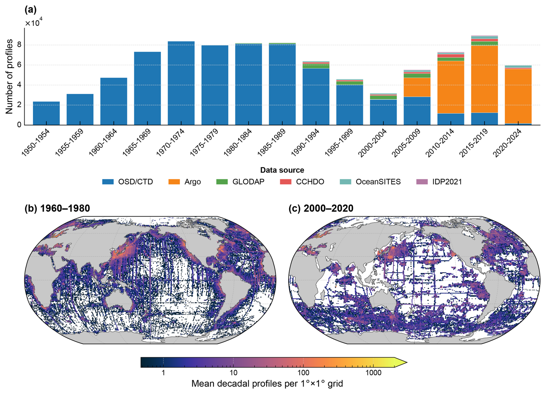
Figure 1 Global distribution and temporal coverage of DO profiles. (a) Changes in the number of profiles from major data sources during 1950–2024. (b–c) Spatial distribution of decadal-mean profile counts for 1960–1980 and 2000–2020, computed on a 1° × 1° grid. The color bar indicates the decadal-mean number of profiles per grid cell (log scale). G24 denotes the oxygen compilation of Gouretski et al. (2024).

After two-stage QC, we assembled a high-quality archive of 930 252 DO profiles, of which 94 % are derived from the OSD, CTD, and Argo platforms. Figure 1a captures the decisive transition in the historical data record: a long-standing reliance on ship-based OSD and CTD profiles was superseded post-2000 by the exponential growth of the Argo network, which now serves as the backbone of global oxygen monitoring. Platform-specific dominance is also depth-dependent, defining the vertical representativeness of the dataset. Above 800 m, the combined prevalence of OSD, CTD, and Argo remains robustly above 90 %. However, the intermediate depths (800–1800 m) mark a transitional zone where Argo's increasing share compensates for the thinning OSD/CTD coverage. Beyond 2000 m, where Argo penetration is limited, the deep-ocean constraint returns to the OSD and CTD platforms, which maintain a prevalence of at least 80 %. This tiered vertical structure ensures that secondary data products remain supplementary to the core observational framework.

The geometric evolution of sampling has shifted from ship-track-oriented linear clusters to a near-planar global distribution. This shift is most evident in the Southern Hemisphere, where coverage increased from extreme sparsity prior to 1980 to approximately 36 % of the global total in the 2000–2020 interval. This globalization of the data stream, driven by the Argo array, has mitigated historical hemispheric imbalances, although systematic gaps persist in marginal seas, the central Pacific, and ice-influenced Arctic regions.

Acknowledging that uneven observational density poses a risk of artificial signal dominance from high-coverage eras, our methodology incorporates specific safeguards to ensure trend stability. By adopting heterogeneity-based partitioned modeling and decadal-scale transferability assessments, we reduce the risk of data-sparse regions being dominated by modern sampling patterns. These efforts are further supported by an inverse-density weighting scheme and the use of grid-representative values, which together enhance the influence of sparse historical records and maintain the physical interpretability of multi-decadal oxygen trends.

2.2 Feature Data

Accurate reconstruction of ocean deoxygenation needs both long, dense DO observations and drivers that describe physical transport and biogeochemical processes across scales (Oschlies et al., 2018). Consequently, we leverage three-dimensional thermodynamic fields (temperature and salinity) alongside a curated suite of sea surface environmental variables (SSEVs) to establish a process-based predictor space (Table 1).

Table 1 Details of the Feature Data.

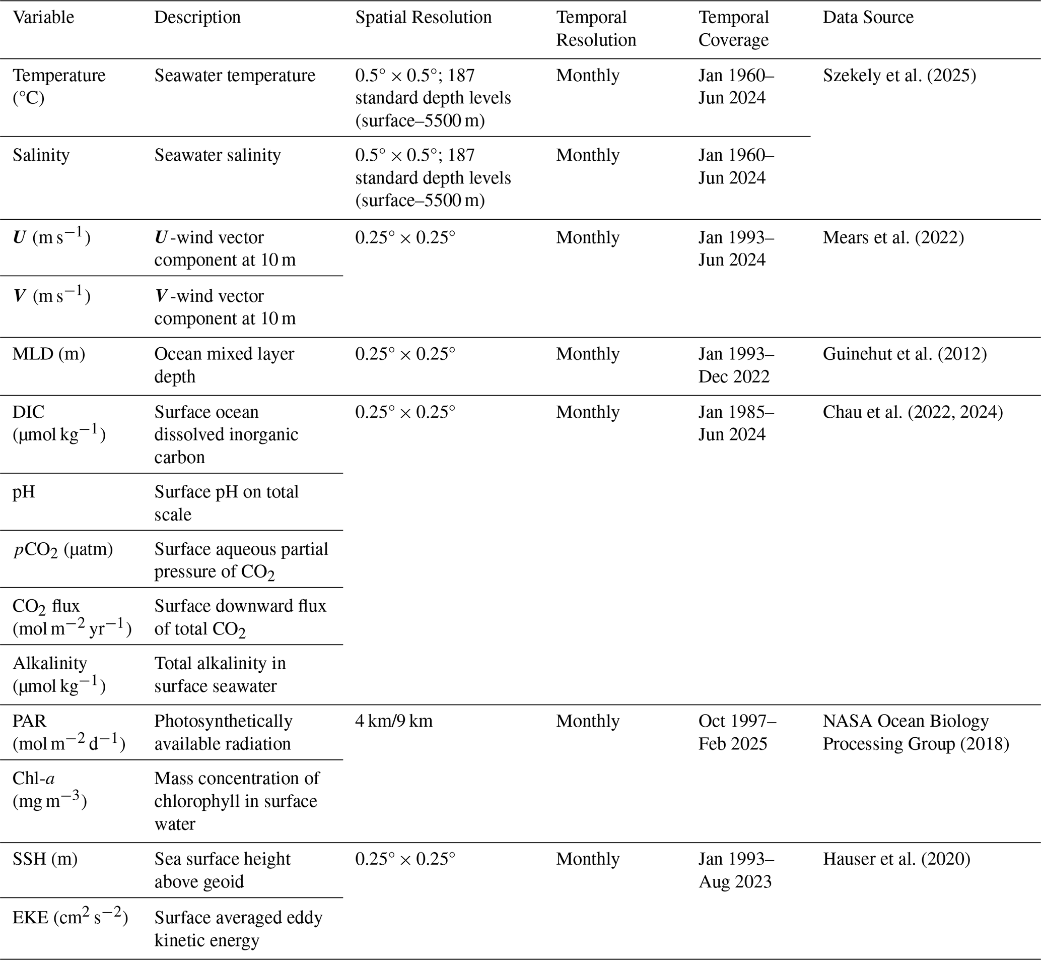
Three-dimensional temperature and salinity fields are taken from the Coriolis Ocean Dataset for Reanalysis, CORA (Szekely et al., 2025). CORA is a CMEMS objective analysis that uses the ISAS objective mapping system to merge in situ temperature and salinity observations from ships, Argo floats, and other platforms. It also applies delayed mode quality control to support long-term stability and global consistency. From these fields, oxygen saturation (O₂Sat) is derived according to the TEOS-10 standard (IOC et al., 2015). The resulting discrepancy between observed DO and O₂Sat serves as a critical proxy for the integrated influence of microbial respiration and physical ventilation dynamics.

Complementarily, we assembled a multidimensional suite of SSEVs, encompassing thermodynamic, dynamical, bio-optical, and carbon-chemistry features (Shao et al., 2024; Ma et al., 2025). Wind-vector components (U and V) are taken from NASA's Cross-Calibrated Multi-Platform (CCMP) product (Mears et al., 2022). Mixed-layer depth (MLD) is obtained from the CMEMS Multi-Observation Global Ocean 3D product (Guinehut et al., 2012). Dynamical variables include sea surface height (SSH) and eddy kinetic energy (EKE), both derived from AVISO satellite altimetry (Hauser et al., 2020). Bio-optical variables comprise photosynthetically active radiation (PAR) and chlorophyll a (Chl-a) from NASA Level-3/Level-4 ocean-color products (NASA Ocean Biology Processing Group, 2018). Carbon-chemistry variables include dissolved inorganic carbon (DIC), total alkalinity, pH, sea surface partial pressure of CO₂ (pCO₂), and CO₂ flux, all obtained from the CMEMS Surface Ocean Carbon Fields product (Chau et al., 2022, 2024). All feature variables, last accessed in March 2025, were standardized onto a uniform monthly 0.5° grid to maintain spatial consistency across the reconstruction.

3 Method

The overall workflow for constructing the GEOXYGEN dataset is illustrated in Fig. 2, comprising data collection and preprocessing, heterogeneity-based partitioning, and model training with integrated physical and biogeochemical predictors. By incorporating a spatial clustering descriptor that captures the large-scale background structure, and depth-/region-adaptive feature selection, we implement a biogeochemistry-aware machine-learning workflow for gridded DO reconstruction.

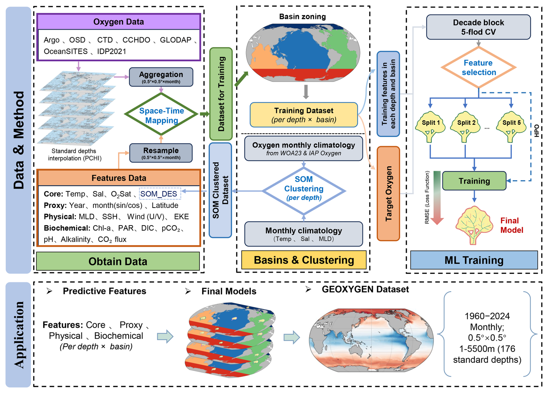
Figure 2 Overall workflow of the GEOXYGEN dataset construction.

3.1 Gridding and Aggregation

To match the spatiotemporal scale of the supervised learning labels with the target reconstruction grid and to reduce sample-weight bias caused by uneven sampling in space and time, all observations are aggregated to a monthly 0.5° by 0.5° grid. Within each grid cell, observations are summarized into a single representative value, defined as the median to limit the influence of outliers and extreme events on the labels. The within-unit dispersion is also computed using the median absolute deviation (MAD), which serves as an empirical proxy for uncertainty.

To quantify representativeness error introduced by finite sampling and sub-grid variability within each cell-month-depth unit, within-unit dispersion is used to estimate σ_rep. Let a unit contain n_obs observations $\mathit{\{}{x}_i{\mathit{\}}}_{i=\mathrm{1}}^{n_{\mathrm{obs}}}$. The representative value is defined as the robust central statistic, as shown in Eq. (3). We then compute the dispersion and define it as the representativeness error metric, σ_rep, as described in Eq. (4), where the factor 1.4826 makes σ_rep comparable to the standard deviation under an approximate normal distribution, facilitating comparison across units.

$$\begin{array}{}\text{(3)}& {\displaystyle }\stackrel{\mathrm{̃}}{x}=\mathrm{median}\left(x_i\right)\text{(4)}& {\displaystyle }\mathrm{MAD}=\mathrm{median}\left(\left|{\mathrm{x}}_i-\stackrel{\mathrm{̃}}{x}\right|\right),{\mathit{\sigma }}_{\mathrm{rep}}=\mathrm{1.4826}\times \mathrm{MAD}\end{array}$$

At the same spatiotemporal scale, all environmental variables and DO data are mapped in space and time. To preserve historical information, all QC-passed DO data are retained even when some covariates such as SSEVs are missing. This sample archive provides standardized inputs for later model training.

3.2 Heterogeneity-Based Partitioning

Our reconstruction framework utilizes a spatiotemporally stratified approach to address the shifting controlling mechanisms of ocean deoxygenation across basins and depths (Ma et al., 2025; Ito et al., 2024a). Following the basin definitions in the World Ocean Atlas 2023 (WOA23; Garcia et al., 2024), we additionally treat the Southern Ocean as a dedicated domain. Accordingly, the horizontal grid is divided into five primary modeling domains (Atlantic, Pacific, Indian, Southern, and Arctic), which are held constant across vertical layers to maintain training coherence (Fig. 3). By avoiding highly intricate province boundaries, this design reduces sensitivity of variability and trend estimates to boundary effects and makes cross-boundary continuity easier to maintain. We further mask the Mediterranean, Red Sea, and other semi-enclosed marginal seas to focus the reconstruction on open-ocean dynamics dominated by large-scale circulation and transport.

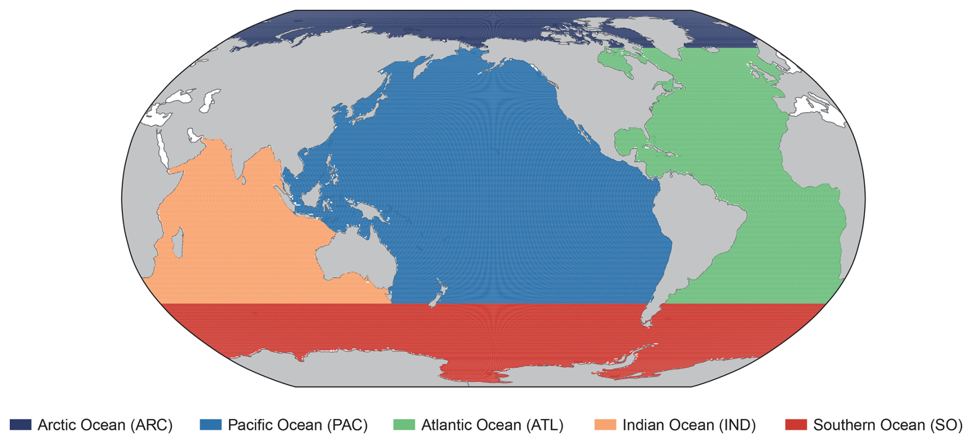
Figure 3 Partitioning of the global open ocean into five basins.

The vertical architecture utilizes 176 standard levels, as discussed in Sect. 2.1, similar to the CORA/ISAS17 frameworks (Szekely et al., 2019; Kolodziejczyk et al., 2023). At each standard depth below 3000 m, the framework converges into a single global model, a necessary adaptation to accommodate the physical constraints of the seafloor and data limitations. For each basin and depth layer, separate models are trained based on the partitioned regions.

Within each depth, the self-organizing-map-derived descriptor (SOM_DES) is used as a categorical predictor to encode the large-scale climatological background state. Specifically, we construct a four-dimensional climatological vector [SST, SSS, MLD, DO] from monthly background fields. These vectors are then used to train a self-organizing map (SOM), and each grid cell is assigned to one of 25 discrete classes. The clustering is based on the joint patterns of multiple environmental fields, and, at this step, the O₂ climatology is implicitly assigned a higher weight to obtain a seasonally varying, dynamic partitioning. The SOM is trained directly on these monthly climatological fields, such that the DO climatology implicitly exerts a stronger influence on the resulting state partition and ensures that the partitioning evolves coherently with the seasonal DO cycle. This feature-engineering step leverages the SOM's ability to map multivariate climatological structure onto a discrete set of regimes while preserving topological dependencies, thereby providing clear seasonal and spatial context for month-scale DO reconstruction. The background climatological fields are anchored in WOA23 (upper 1500 m) and the IAP Global Ocean Oxygen gridded product (IAP Oxygen; Cheng and Gouretski, 2024), ensuring vertically and horizontally comprehensive baseline states. Overall, SOM_DES captures the large-scale climatological structure of DO and supplies background-state information that supports refined month-scale DO modeling, improving diagnostic consistency across heterogeneous regimes and reinforcing the physical interpretability of the global DO product.

3.3 Adaptive Regional Modeling

We train independent sub-models for each ocean basin partition across 176 standard depth levels, employing the CatBoost gradient boosting framework to resolve the non-linear mapping between sparse DO observations and diverse environmental predictors. CatBoost's implementation of oblivious decision trees and ordered boosting is strategically utilized to mitigate variance while precluding target leakage – a critical requirement for stable multi-decadal reconstruction. This framework is algorithmically predisposed to this task due to its innate capacity to process missing predictors without imputation, its support for cost-sensitive sample weighting, and its robust regularization suite (L2 leaf regularization and early stopping) that safeguards against overfitting in data-sparse regimes.

During the period before the satellite era (for example, from the 1960s to the 1980s), this model would automatically identify and properly handle the missing SSEVs. This non-imputational strategy allows the reconstruction to hinge predominantly upon thermodynamic variables (Temperature, Salinity, O₂Sat) and spatiotemporal coordinates without introducing the systematic biases inherent in statistical filling. We tested longitude as a candidate predictor; however, it induced spurious banded (stripe-like) artifacts in data-sparse regions and was therefore excluded from the final predictor set. The CatBoost model uses 20 predictor variables as inputs: Year, month_sin, month_cos, Latitude, Temperature, Salinity, O₂Sat, SOM_DES, U, V, SSH, EKE, MLD, PAR, Chl-a, DIC, pCO₂, pH, Alkalinity, and CO₂ flux. The month_sin and month_cos encodings are defined in Eqs. (5)–(6).

$$\begin{array}{}\text{(5)}& {\displaystyle }\mathrm{month}\mathrm{\_}\sin =\sin \left({\displaystyle \frac{\mathrm{2}\mathit{\pi }(m-\mathrm{1})}{\mathrm{12}}}\right)\text{(6)}& {\displaystyle }\mathrm{month}\mathrm{\_}\cos =\cos \left({\displaystyle \frac{\mathrm{2}\mathit{\pi }(m-\mathrm{1})}{\mathrm{12}}}\right)m\in \mathit{\{}\mathrm{1},\mathrm{2},\mathrm{\dots },\mathrm{12}\mathit{\}},\end{array}$$

To improve interpretability and generalization, a two-stage feature selection procedure is applied to each region–depth submodel. Only training data are used, and cross-validation follows the same decadal-scale design used for model evaluation. Tree-based models often benefit from compact feature sets because redundant predictors can reduce predictive skill (Garabaghi et al., 2023). First, we estimated permutation importance under five-fold cross-validation grouped by decade and retained an initial subset of features using an adaptive rule $K=max(\mathrm{10},\mathrm{2}\sqrt{p})$, where p=20 is the number of candidate features, discarding predictors with negligible contribution. Second, we perform recursive feature elimination with cross-validation (RFECV), iteratively removing the least important feature and selecting the combination that minimizes validation Root Mean Square Error (RMSE). This process facilitates a physical evolution of the feature space: surface models prioritize high-frequency biogeochemical forcing, mid-depth models emphasize water-mass transition markers, and deep-ocean models converge on conservative thermodynamic tracers.

To mitigate biases arising from heterogeneous spatiotemporal sampling (Fig. 1), we applied inverse-density weighting within a fixed binning scheme. The sample domain is partitioned on a 5° × 5° latitude–longitude grid and non-overlapping 10-year time windows in each cell. Sample weights were computed as the inverse of the observational density within each spatiotemporal bin and standardized at each depth level, thereby reducing the influence of over-sampled regions and periods during model training.

Let b(i) denote the spatiotemporal bin containing sample i, and let n_b(i) be the number of samples in that bin. The initial per-sample weight is the inverse square root of this count, as defined in Eq. (7).

$$\begin{array}{}\text{(7)}& {\stackrel{\mathrm{̃}}{w}}_i={\displaystyle \frac{\mathrm{1}}{\sqrt{n_{b\left(i\right)}}}},\end{array}$$

Specifically, each sample weight is set proportional to the inverse square root of the local sample density. To preserve the aggregate information content, we then normalize the weights to unit mean, as defined in Eq. (8).

$$\begin{array}{}\text{(8)}& w_i={\displaystyle \frac{{\stackrel{\mathrm{̃}}{w}}_i}{\frac{\mathrm{1}}{N}\sum _{k=\mathrm{1}}^N{\stackrel{\mathrm{̃}}{w}}_k}},\end{array}$$

This strategy increases the influence of observations from sparse regions and earlier periods without altering the aggregate sample distribution.

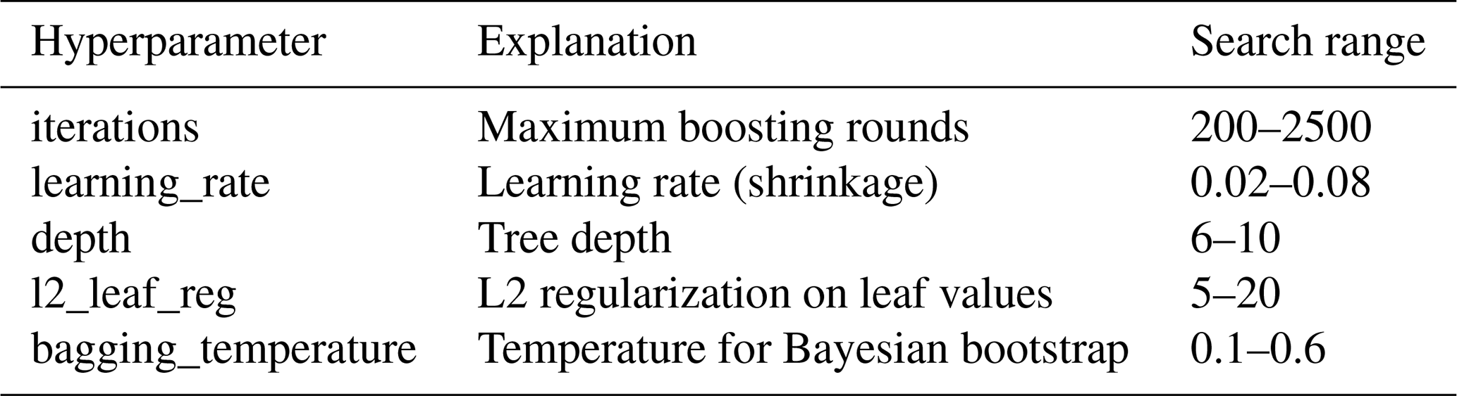
3.4 Hyperparameter optimization and validation

Independent hyperparameter optimization for each basin-depth unit is performed using Bayesian inference (Optuna), targeting the objective of validation RMSE minimization (Table 2). This automated search is integrated with a decadal-block five-fold cross-validation scheme to address the challenges of non-stationary ocean signals. By grouping observations into multi-year blocks, we decouple validation results from the short-term temporal dependencies that often inflate predictive skill in traditional random-split CV (Salazar et al., 2022). This structural separation ensures that the model learns large-scale climatic drivers rather than localized temporal artifacts. In each cross-validation fold, early stopping is activated if validation RMSE fails to improve for 50 consecutive iterations, after which the optimal iteration count is recorded. To secure a robust final model, we set the terminal iteration count to the median of these recorded values across all folds. This iteration-locked retraining on the complete calibration set – with early stopping disabled – prevents overfitting and ensures a stable convergence state.

Table 2 CatBoost hyperparameters and Optuna search priors.

For an unbiased final assessment, a strictly independent global test set is constructed via decade-stratified random sampling (1960–2024), where one full calendar year per decade is entirely excluded from feature selection and hyperparameter tuning. The resultant test years (1961, 1970, 1984, 1993, 2003, 2012, and 2020) provide a temporally representative benchmark. This withheld-year test set is reserved exclusively for final performance assessment and inter-product benchmarking; all model selection and calibration are conducted via decade-block cross-validation within the remaining training data. Integrated predictions from regional sub-models are then evaluated against this set using RMSE, mean absolute error (MAE), and the coefficient of determination (R²).

4 Results

4.1 Variable Associations and Feature Contributions

The relationship between DO and its environmental drivers undergoes a transformation from the surface to the deep ocean (Fig. 4). In the near-surface layers, thermodynamic solubility constraints dominate, manifesting as a robust negative correlation with temperature. As depth increases, this direct solubility control attenuates, allowing salinity to emerge as the primary integrative proxy for water-mass properties and ventilation history, particularly tracking the signatures of deep-water formation and transport. These depth-dependent patterns provide the empirical foundation for resolving complex non-linear interactions within the water column (Ping et al., 2024; Cao et al., 2024).

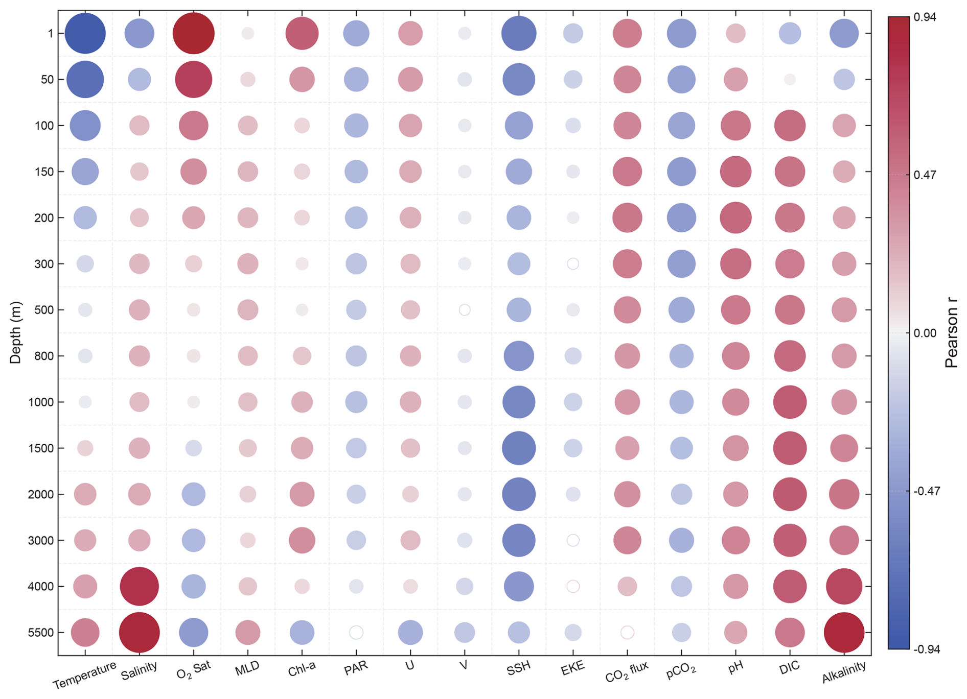
Figure 4 Vertical correlations between DO and physical–biogeochemical variables. Bubble color encodes the sign and magnitude (red = positive; blue = negative), and bubble area scales with ($\left|r\right|$). Filled bubbles denote correlations significant at (q<0.05) after Benjamini–Hochberg false-discovery-rate control; hollow bubbles indicate non-significant results.

Correlations between sea surface environmental variables (SSEVs) and subsurface DO represent teleconnected pathways rather than local drivers. Surface dynamical forcing and upper-ocean mixing modulate water-mass formation and reventilation, thereby constraining the DO budget at depth. Specifically, sea surface height (SSH) exhibits persistent vertical coherence across much of the water column, while wind stress provides a dynamical context for advection and upwelling (Hollitzer et al., 2024). In contrast, the Chl-a signal remains confined to the epipelagic zone, reflecting its role as a productivity indicator. Beyond the euphotic zone, carbonate system variables, notably alkalinity, maintain high correlations with DO, delineating the remineralization background linked to deep-water aging.

Feature-importance diagnostics are reported to describe model dependence and do not imply causality. The adaptive feature-selection results show that the model's reliance on predictors varies strongly with depth and region. In the upper 10 m, temperature and O₂ saturation are consistently among the most informative predictors, whereas at intermediate depths (1000–2000 m) salinity tends to contribute more strongly in certain high-latitude regimes, including the Arctic and Southern Oceans (Fig. 5). This depth-dependent pattern motivates the use of depth-specific predictor sets to better represent distinct hydrographic contexts. In addition, several regionally relevant covariates (e.g., SSH in the Indian Ocean and DIC/alkalinity in low-oxygen environments) are retained more frequently by the selection procedure, indicating that they provide useful contextual information for prediction under specific regimes (Franco et al., 2014).

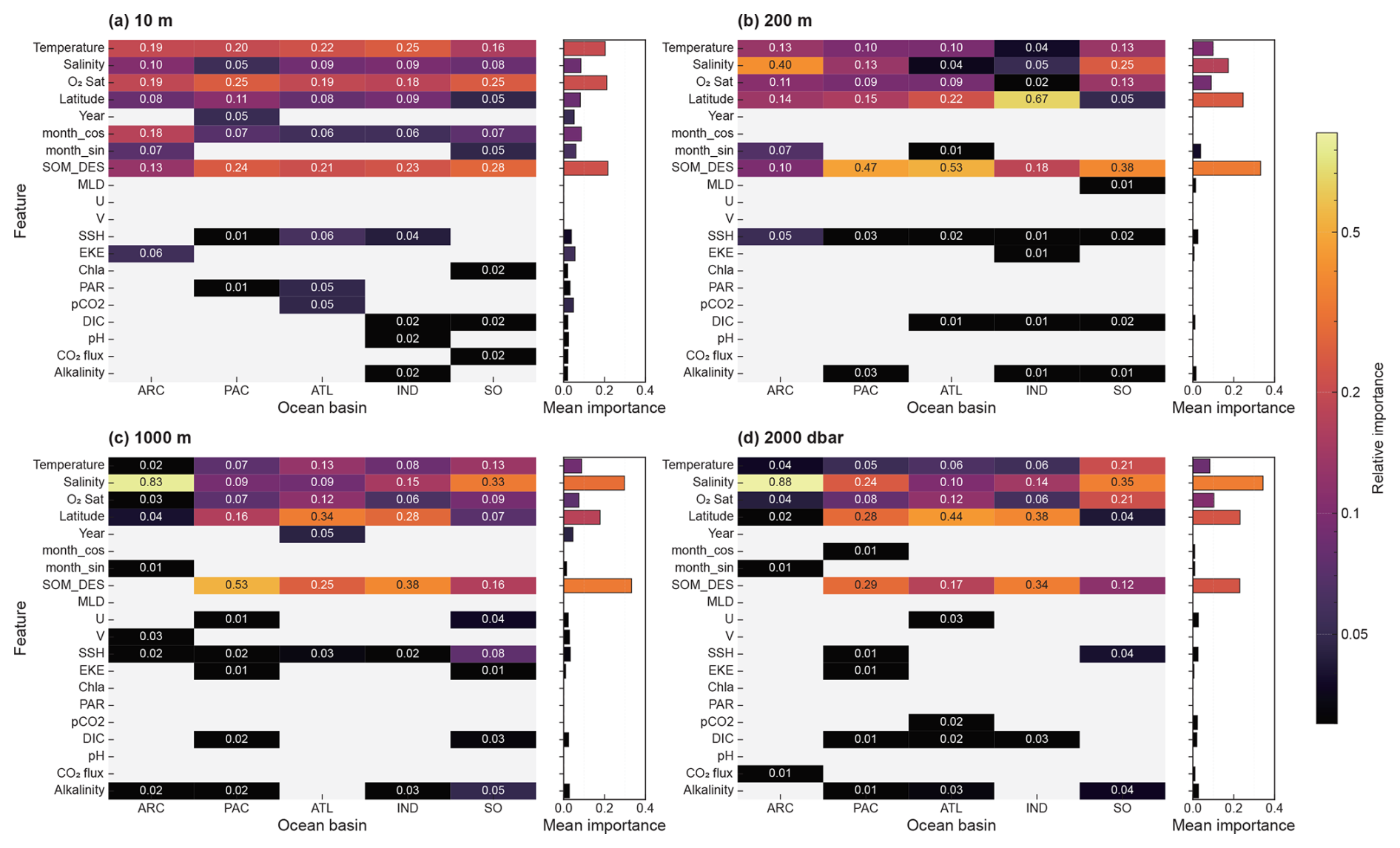
Figure 5 Heatmap of relative feature importance across depths and basins. Colors are on a logarithmic scale. The bar chart on the right shows each feature's mean importance computed over the basin provinces in which that feature is available.

Although latitude serves as a dominant proxy for broad-scale gradients (Milà et al., 2024), specialized SSEVs are vital for refining local accuracy. Our regionalized architecture prioritizes these idiosyncratic dynamics, utilizing variables like SOM_DES to resolve high-frequency seasonal variations in the Southern Ocean. This adaptive approach mitigates the biases inherent in spatially stationary parameterizations, ensuring the reconstruction respects the intrinsic heterogeneity of the global oxygen cycle.

4.2 Model evaluation

Vertical stratification of error profiles reveals a coherent link between RMSE and the intensity of the oxycline (Fig. 6). In most basins, uncertainty is concentrated in the upper 600 m, where biological consumption and physical mixing generate high spatiotemporal variance. The Indian Ocean (IND) presents the most significant upper-ocean RMSE peak, likely due to its unique biogeochemical configuration, whereas the Arctic Ocean (ARC) shows fluctuations in RMSE at intermediate depths, but its R² remains relatively high. This vertical decoupling of error – where water-mass stability increases with depth before decreasing – represents a common feature across the Atlantic, Pacific, IND, and Southern Oceans, further confirming the appropriateness of the regional partitioning approach.

Figure 6 Depth profiles of model performance across basin provinces.

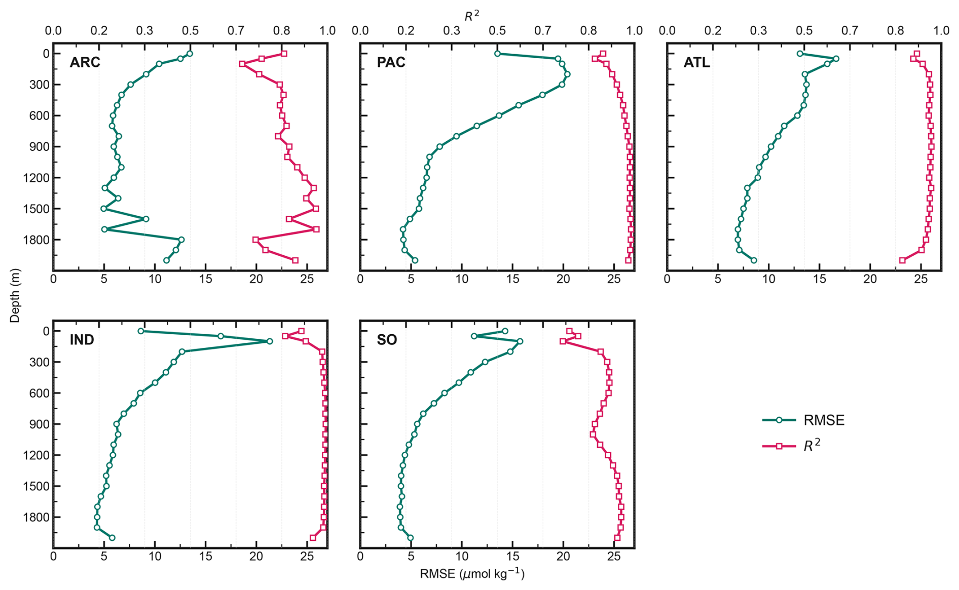
Except for the sparsely sampled Arctic, all ocean basins maintain high R² values (typically > 0.8) across the sampled water column. While absolute errors are inherently higher in the upper ocean where DO variability is maximized, the high R² values indicate that the underlying spatial and temporal patterns are accurately recovered. The analysis demonstrates that uncertainty is largely a function of the vertical DO structure, with the deep-ocean regime providing a stable and highly predictable anchor for long-term deoxygenation trends.

The reconstructed DO fields demonstrate high accuracy throughout the global ocean, with scatter plots confirming that estimates follow the 1 : 1 line across the entire concentration range (Fig. 7). At representative depths, the global RMSE/MAE on the independent test set is on the order of 12.8/8.0 µmol kg⁻¹ at 10 m, 16.8/11.4 µmol kg⁻¹ at 200 m, and 7.5/5.2 µmol kg⁻¹ at 1000 m. Most R² values are above 0.9, and the R² for deep-layer DO reconstruction reaches 0.99. A slight overestimation in regions with relatively low values reflects the inherent smoothing characteristic of regularized decision trees, which tend to pull extreme values toward local means. However, the symmetric distribution of residuals around zero indicates that these effects are localized and do not introduce a systematic large-scale bias. This performance confirms that the modeling architecture is well-suited for resolving the non-linearities inherent in ocean oxygen dynamics.

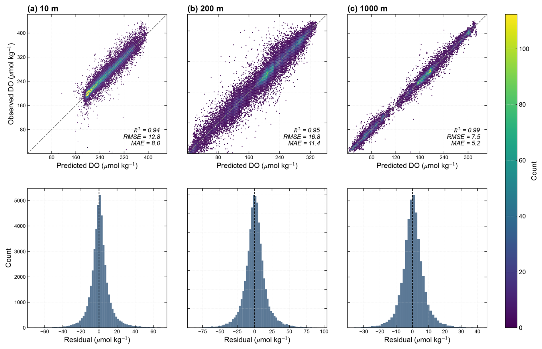
Figure 7 Model performance for DO predictions across depth layers (independent test set). Top row: hexagon-binned scatterplots of predicted vs. observed values; the gray dashed line denotes the 1 : 1 reference. The color bar indicates sample counts per hexbin. Bottom row: corresponding histograms of residuals (observed − predicted).

4.3 Long-term dataset

The trained models leverage CORA ocean analysis from CMEMS to generate spatially and temporally consistent monthly dissolved oxygen (DO) reconstructions. By using gridded temperature and salinity products, the framework obviates interpolation from sparse in situ profiles and minimizes associated uncertainties. These predictors undergo delayed-mode objective mapping and rigorous quality control to ensure long-term consistency and full traceability. Monthly DO predictions are generated at 176 standard depth levels on a 0.5° × 0.5° grid extending to 5500 m.

To mitigate discontinuity artifacts at basin province boundaries – described as the “step-effect” – a boundary fusion protocol is implemented within transition zones (Wagstaff and Bean, 2022). For a prediction location x, the fused estimate is derived from the regional model prediction ${\widehat{y}}_i\left(\mathit{x}\right)$ and the minimum great-circle distance d_i to the provincial boundary, as defined in Eq. (9). With a smoothing bandwidth of S=300 km, predictions from adjacent basins are smoothly blended in proportion to their distance from the edge. This approach preserves continuity across boundaries without excessive smoothing. Far from boundaries (d>S), only the local provincial model contributes to the estimate.

$$\begin{array}{}\text{(9)}& \begin{array}{rl}& {\widehat{y}}^{\prime }\left(\mathit{x}\right)={\displaystyle \frac{{\sum }_{i}w\left(d_i\mid S\right){\widehat{y}}_i\left(\mathit{x}\right)}{{\sum }_{i}w\left(d_i\mid S\right)}},\\ & w\left(d_i\mid S\right)=\left\{\begin{array}{ll}{\left(\frac{\left(S-d_i\right)}{S}\right)}^{\mathrm{2}},& d_i\le S\\ \mathrm{0},& d_i>S\end{array}\right.,\end{array}\end{array}$$

Finally, we obtained GEOXYGEN, a global DO dataset that provides monthly fields on a 0.5° × 0.5° latitude–longitude grid at 176 standard depth levels from 1 to 5500 m, spanning 1960–2024. The latitude grid is not strictly uniform, with higher density in the high-latitude regions. Distributed via CF-compliant NetCDF files, each monthly volume (GEOXYGEN_DO_YYYYMM_0p5deg_v1.nc) includes the four-dimensional DO variable (time × depth × lat × lon) and associated coordinates. Time represents monthly means encoded as days since 1 January 1950 00:00:00 UTC (Gregorian calendar), with missing data identified by a large sentinel value. A separate NetCDF file provides the basin provinces and valid-ocean masks. The complete dataset is available at https://doi.org/10.12157/IOCAS.20260223.002 (Wang et al., 2026b).

4.4 Comparison with other products

To evaluate the predictive fidelity of GEOXYGEN against four existing dissolved oxygen (DO) products (Table 3), we utilize the independent test dataset stratified across discrete temporal windows: the early period (1960–1980) and the recent epoch (2000–2020; Table 4). The intercomparison is strictly constrained to spatiotemporally co-located samples, ensuring that only grid-month-depth intersections with concurrent availability across all products are included in the evaluation. This rigorous filtering preserves statistical equity and minimizes biases arising from disparate product masks.

Table 3 Summary of our product and other DO products.

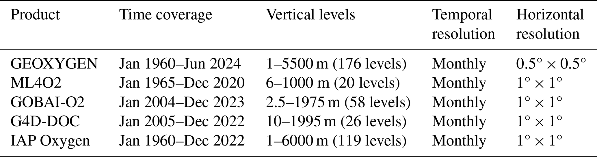
Table 4 Accuracy by depth for each product relative to observations. RMSE and bias are reported in µmol kg⁻¹; R² is dimensionless.

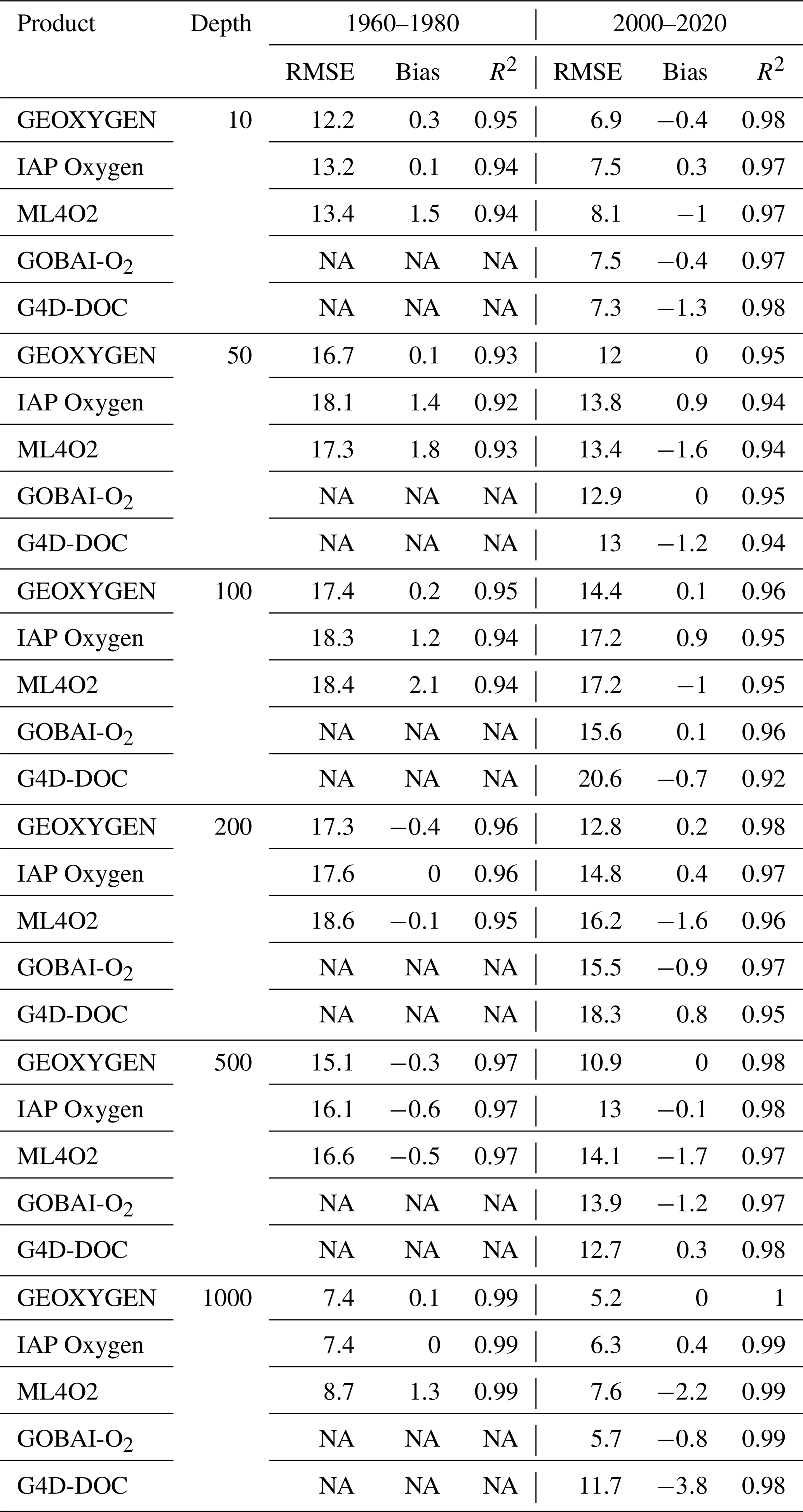
NA – not available.

The comparative analysis reveals three dominant patterns. First, all products show larger errors during the early period, a trend predominantly attributable to the historical sampling architecture. Pre-Argo observations were characterized by a disproportionate concentration of coastal and shelf cruises, whereas the modern era is defined by the proliferation of autonomous Argo floats providing expansive open-ocean coverage. Because coastal environments are governed by pronounced small-scale heterogeneity and high-frequency nonstationarity, their reconstruction poses a greater challenge, inherently raising the error floor for the 1960–1980 interval.

Within this data-sparse window (1960–1980), GEOXYGEN manifests superior predictive stability across the upper and intermediate layers (10–500 m). It consistently achieves lower RMSE and MAE than both IAP and ML4O2 across nearly all depth levels while maintaining robust R² values. These gains demonstrate that the stratified, basin-specific modeling framework facilitates the recovery of mesoscale spatial heterogeneities and vertical gradients even under sparse observational constraints. By leveraging high-resolution target fields, this architecture enhances the representation of regional variability, ensuring that GEOXYGEN maintains competitive skill during the pre-satellite and pre-Argo eras.

In the data-rich modern period (2000–2020), GEOXYGEN exhibits even more pronounced performance gains. Within the critical mesopelagic range (100, 200 and 500 m), the product shows a significant accuracy improvement relative to all reference datasets, while ensuring that residual biases are smaller and more stable. In contrast, several existing products exhibit persistent systematic biases in this depth range, potentially compromising the representation of OMZs and steep vertical gradients. This suite of high-resolution, broad-coverage DO fields provides a reliable foundation for the integrated assessment of global deoxygenation trends and their underlying physical-biogeochemical drivers.

4.5 Comparison with WOA23

To evaluate the large-scale credibility and multi-year stability of our reconstructed dissolved oxygen (DO) fields, we compare our product's annual-mean DO climatology with WOA23 and examine vertical structure using representative profiles from three major basins (Fig. 8).

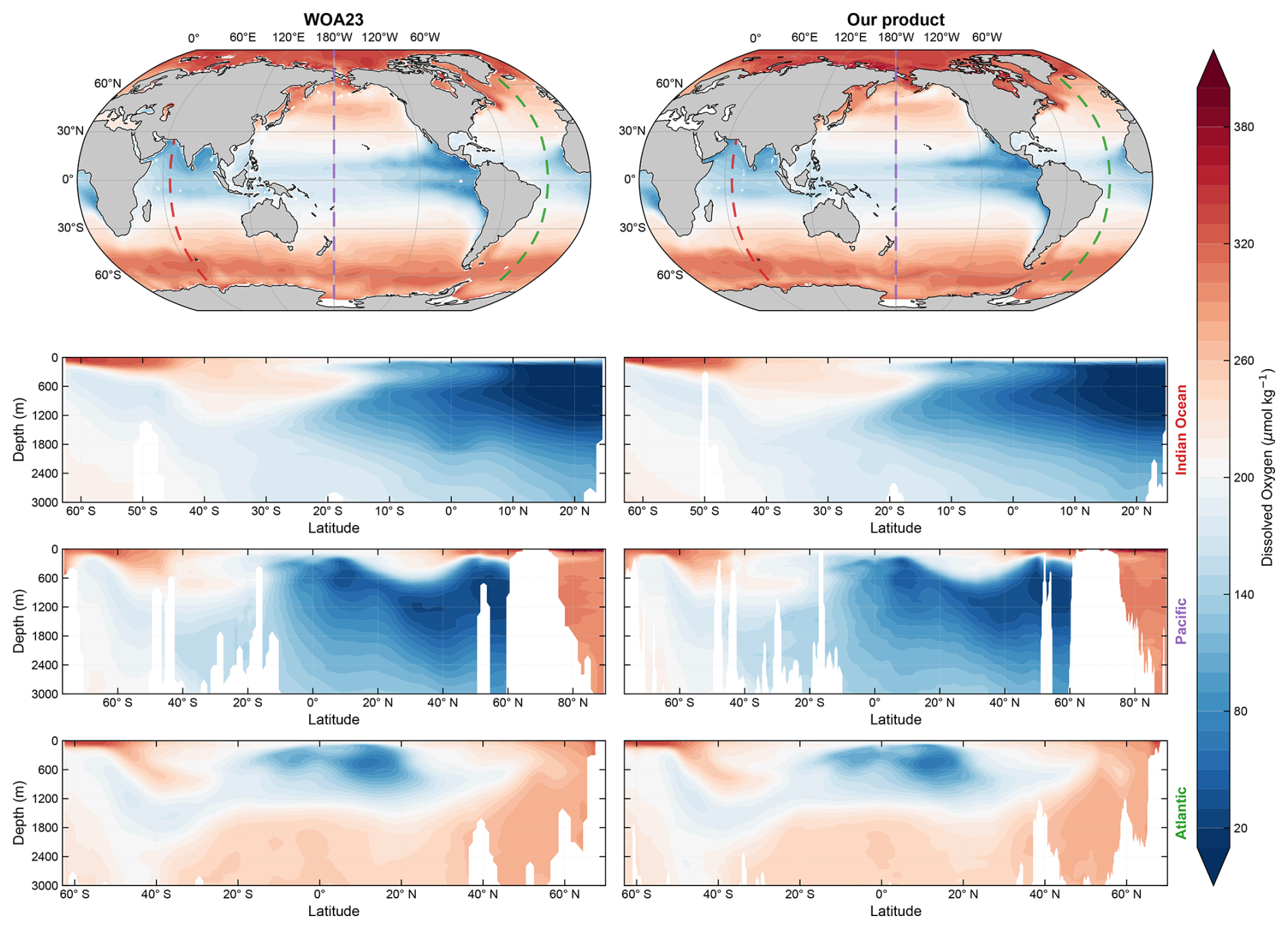
Figure 8 Climatological comparison between WOA23 and our product (GEOXYGEN). Row 1 shows the global-mean DO distribution averaged over 0–300 m. Colored dashed lines mark the locations of three sections: 65° E (red), 180° W (purple), and 30° W (green). Rows 2–4 show DO cross-section distributions along these three transects.

In the upper ocean (0–300 m, depth-averaged), both products capture consistent basin-scale spatial patterns. The subtropical gyres exhibit relatively high DO concentrations, while the equatorial region and eastern boundary upwelling systems form distinct oxygen-deficient belts. The spatial extent and location of these structures are in close agreement between the two climatologies. GEOXYGEN reproduces these banded structures continuously, with cross-frontal gradients in transition zones closely matching those in WOA23.

In the vertical, our product accurately depicts the largest hypoxic zone in climatology, which is mainly located in the intermediate depth, ranging from 300 to 1300 m. Meridional sections reveal that the model successfully reproduces the core depths and spatial extents of major hypoxic zones across the three primary ocean basins. The precise alignment of oxygen isopleths and the accurate representation of the transition layer steepness indicate that the reconstruction results are consistent with the climatological constraints of DO.

Unlike the standard 1° grid used in most global products, GEOXYGEN employs a higher 0.5° horizontal resolution to capture more detailed features. By training on localized relationships between DO and hydrographic analyses within discrete basin provinces, the model resolves the morphometry of OMZs with enhanced clarity. Although the reconstruction fidelity remains conditioned upon the quality of input observations, benchmarking against 1° products reveals that the 0.5° configuration yields systematically lower errors in high-gradient regimes. This selection constitutes an optimized operating resolution that maximizes information recovery from the underlying biogeochemical constraints without over-interpreting sparsely sampled intervals.

5 Discussion

5.1 Uncertainty Analysis

To quantify the credibility of the GEOXYGEN product, we decompose total uncertainty into two components: observation-related uncertainty and mapping uncertainty. Observation-related uncertainty summarizes measurement error and the representativeness error introduced when observations are aggregated to the cell–month–depth scale. Mapping uncertainty describes prediction error from the machine-learning mapping between environmental predictors and DO. This decomposition separates label-side and model-side contributions. It also supports diagnosing elevated uncertainty in coastal regions and potential bias in earlier, data-sparse periods, and it improves traceability and clarity for product use.

Measurement error depends on the measurement technique and instrument. For Winkler titration, bottle measurements can include random errors on the order of 1 µmol kg⁻¹ or smaller (Carpenter, 1965). Since observing platforms differ in sensor type, calibration strategy, and QC level, we assign a platform-specific measurement error scale σ_meas to each data source to represent differences in precision among platforms. Bottle-based sources including CCHDO Bottle, GLODAP, and GEOTRACES IDP are assigned 1 µmol kg⁻¹. Since Argo data are bias corrected, Argo, OSD and CTD, and CCHDO CTD are assigned 1.5 µmol kg⁻¹. OceanSITES is assigned 2.0 µmol kg⁻¹.

When forming supervised-learning labels at the cell–month–depth scale, observation-related uncertainty is defined as the combined contribution of measurement error, vertical mapping uncertainty, and representativeness error, as defined in Eq. (10).

$$\begin{array}{}\text{(10)}& U_{\mathrm{obs}}=\sqrt{{\mathit{\sigma }}_{\mathrm{meas}}^{\mathrm{2}}+{\mathit{\sigma }}_{\mathrm{interp}}^{\mathrm{2}}+{\mathit{\sigma }}_{\mathrm{rep}}^{\mathrm{2}}}\end{array}$$

Here, σ_interp is the vertical mapping uncertainty introduced when a profile is mapped to standard levels, and σ_rep is the representativeness error estimated from within unit dispersion. Their definitions and computation have been described earlier.

Mapping uncertainty characterizes error generated during the mapping from environmental fields to DO. It reflects the combined effects of model structure, representativeness of training samples, and nonstationarity across regions and depth levels. On the independent test set, we define the residual following Eq. (11):

$$\begin{array}{}\text{(11)}& r=\widehat{y}-y\end{array}$$

where $\widehat{y}$ is the model prediction and y is the observed label for the corresponding test sample. Following Ito et al. (2024a), we estimate the mapping uncertainty at each grid cell from the test residuals by taking their second central moment, as defined in Eq. (12).

$$\begin{array}{}\text{(12)}& {\mathit{\sigma }}_{\mathrm{map}}=\sqrt{{\stackrel{\mathrm{‾}}{r}}^{\mathrm{2}}-{\left(\stackrel{\mathrm{‾}}{r}\right)}^{\mathrm{2}}},\end{array}$$

Here, the overbar denotes the mean over all test samples within the same grid cell. This definition estimates the residual variance at the grid cell scale. It separates the systematic component $\stackrel{\mathrm{‾}}{r}$ from the random error component captured by σ_map.

Based on the two components above, total uncertainty (U_total) is defined in Eq. (13).

$$\begin{array}{}\text{(13)}& U_{\mathrm{total}}=\sqrt{U_{\mathrm{obs}}^{\mathrm{2}}+{\mathit{\sigma }}_{\mathrm{map}}^{\mathrm{2}}}\end{array}$$

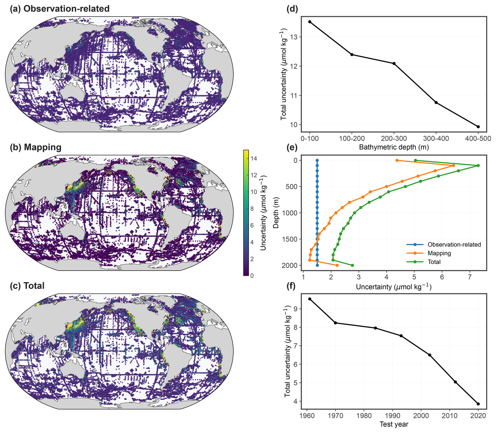
Figure 9 The left panels show the mean uncertainty distributions across multiple standard depth layers (0–2000 m), including observational uncertainty (a), mapping uncertainty (b), and total uncertainty (c). The right panels depict the nearshore spatial variability of total uncertainty (d), its vertical (depth-dependent) structure (e), and the decadal evolution of total uncertainty over the test years (f).

As shown in Fig. 9, the spatial distribution of uncertainty in GEOXYGEN reveals a distinct bifurcation between observation-related uncertainty and mapping residuals. Observational uncertainty manifests pronounced spatial stationarity across pelagic domains. Conversely, mapping uncertainty exhibits a structured regional geometry, with elevated error bands aligning with high-gradient kinetic regimes such as western boundary currents and upwelling systems. The highest uncertainty is observed in the Pacific (7.385 µmol kg⁻¹), followed by the Atlantic (6.148 µmol kg⁻¹), Arctic (4.439 µmol kg⁻¹), Indian (4.084 µmol kg⁻¹), and Southern Ocean (3.652 µmol kg⁻¹). The higher uncertainty in the Pacific and Atlantic Oceans is primarily due to the structural complexity and dynamic intensity of their oceanographic systems, as well as the coastal distribution of early observational data in these basins. The global-mean total uncertainty of 6.054 µmol kg⁻¹ conceals a pronounced shallow-water divergence: in nearshore and shelf regions where bathymetric depth is shallower than ∼ 200 m, total uncertainty rises to 12.917 µmol kg⁻¹ – more than double the open-ocean baseline (5.970 µmol kg⁻¹). Consistent with the bathymetry-binned diagnostic, uncertainty increases monotonically with decreasing bathymetric depth, indicating progressively reduced predictability toward the shallow, dynamically heterogeneous coastal ocean (Fig. 9d). This intensification is predominantly driven by localized, high-frequency processes – including phytoplankton pulses, riverine influx, and tidal oscillation – which generate non-linear spatial gradients that challenge the transferability of pelagic-trained feature relationships (Gilbert et al., 2010; Regier et al., 2023; Giomi et al., 2023; Liu et al., 2024). These localized dynamics induce steep spatial gradients and temporal non-stationarity, which subsequently reduce the regional transferability of learned DO-environment associations (Valera et al., 2020). For nearshore and semi-enclosed bay environments, we recommend using GEOXYGEN with caution and interpreting results at larger spatial aggregation to reduce sensitivity to local high-frequency variability.

The vertical stratification of uncertainty reflects the underlying hydrographic stability and process coupling within the water column. As depicted in Fig. 9e, the total uncertainty profile reaches its maximum in the epipelagic layer before undergoing monotonic attenuation toward the abyssal depths. This vertical variation is consistent with the change in model accuracy across depth layers. In contrast, the intermediate and deep layers provide stronger water-mass constraints and a more coherent oxygen field, facilitating a convergence of mapping uncertainty as the predictive relationship stabilizes.

Temporal trends in uncertainty serve as a diagnostic of the evolving global observing system. The progressive reduction in total uncertainty across the withheld test years (Fig. 9f) coincides with the expansion of the Argo float network, which transitioned ocean sensing from route-based ship surveys to a spatially distributed autonomous paradigm. This transition significantly improved the observational constraints in the Southern Hemisphere and remote ocean basins, effectively lowering the residual variance in model validation. While this decline highlights the structural evolution of sampling coverage, the resulting time series reflects the collective stability of the multi-decadal reconstruction rather than a year-specific local error estimate.

It should be noted that GEOXYGEN has higher uncertainty in coastal and shelf regions. Therefore, for coastal applications, we recommend using multi-grid-cell averages and focusing on monthly to seasonal or longer timescales. Use of the native 0.5° grid near the coast should therefore be approached with caution and, wherever feasible, cross-validated against local observations or higher-resolution regional products.

5.2 Impact of Removing Surface Predictors on Trends

A two-configuration sensitivity experiment was designed to test whether satellite-era sea-surface information alters the reconstructed dissolved oxygen (DO) signal. The full predictor configuration used the complete predictor suite, while the reduced predictor configuration excluded the sea-surface predictor group (U, V, SSH, EKE, MLD, PAR, Chl-a, DIC, pCO₂, pH, alkalinity, and CO₂ flux). All other parts of the reconstruction pipeline were kept the same, so differences between the two products isolate the effect of including this predictor group on the same grid and over the same period.

The comparison focuses on deseasonalized DO anomalies averaged over the 1–100 m depth range and further smoothed using a centered 12-month moving average. This metric targets the upper ocean, where sea-surface information is most likely to influence variability, while suppressing grid-scale noise that can obscure low-frequency signals. Predictor impact is quantified by the configuration-induced component, defined as Full − Reduced, which isolates the incremental effect of the excluded predictor group in anomaly space.

The full and reduced reconstructions exhibit strong agreement over 1960–2022 (Fig. 10), yielding a consistent depiction of upper-ocean (1–100 m) low-frequency variability: a sustained positive-anomaly regime through the 1970s–1980s followed by a marked decline after ∼ 1990 and a transition into a persistently negative-anomaly regime by ∼ 2000 (relative to the monthly climatology). The Full–Reduced difference remains close to zero prior to the mid-1980s and stays small compared with the total anomaly amplitude thereafter, indicating that the global-mean, decadal-scale signal is only weakly sensitive to the inclusion of satellite-era surface predictors. As an external benchmark, ML4O2 reproduces comparable variability during ∼ 1965–2010 but shows more negative anomalies in the most recent decade, suggesting a stronger upper-ocean deoxygenation signal in anomaly space (relative to its monthly climatology) than GEOXYGEN over the same period; however, part of this divergence may arise from inter-product differences in baseline climatology, sampling, and reconstruction methodology. Overall, the close concordance between configurations supports the robustness of GEOXYGEN for decadal-scale assessments, with configuration-dependent deviations being minor relative to the dominant multi-decadal evolution.

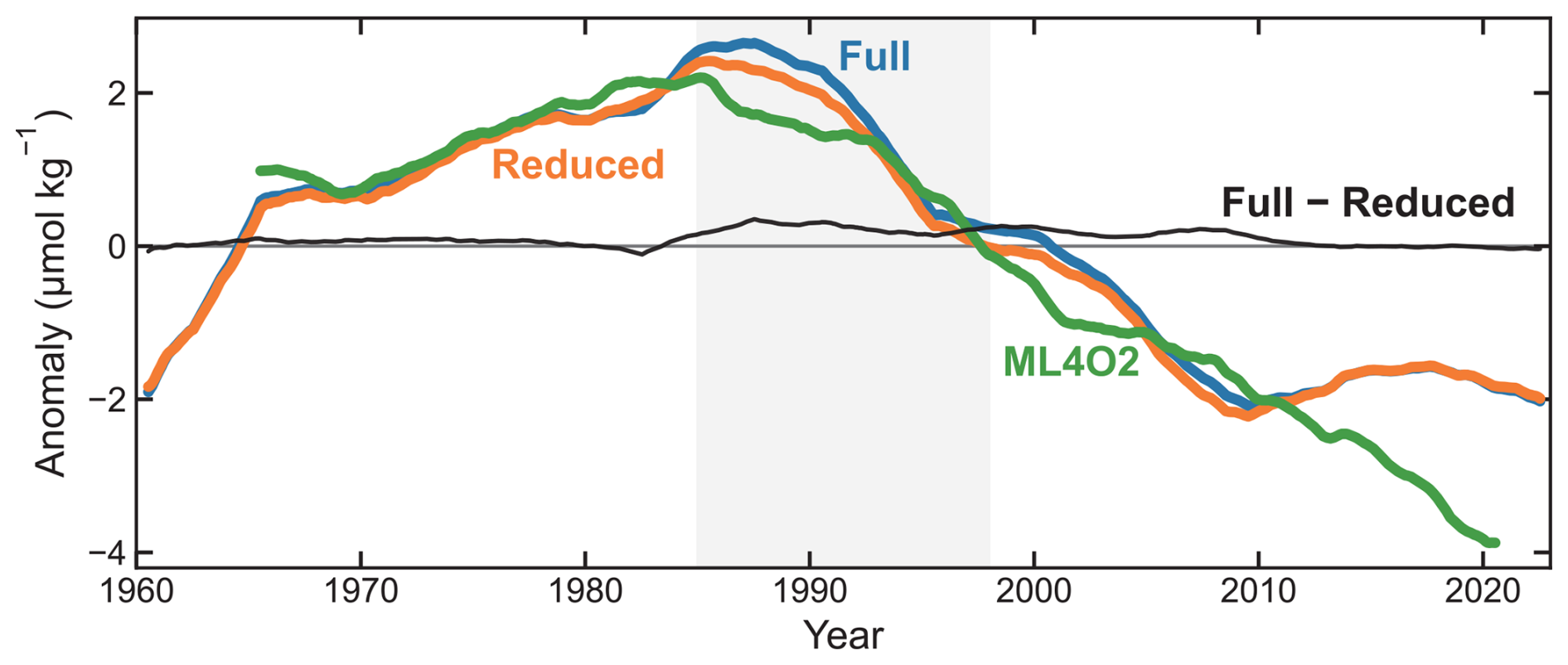
Figure 10 Depth-averaged (1–100 m) monthly dissolved-oxygen anomalies (1960–2022). The figure compares deseasonalized anomalies from the Full predictor reconstruction, the Reduced predictor reconstruction (excluding sea-surface predictors), and ML4O2, and overlays the difference between the Full and Reduced reconstructions (Full − Reduced). Gray shading indicates 1985–1997, corresponding to the rapid expansion of satellite-derived sea-surface observations.

5.3 Ship-Only Analysis of Long-Term Trends

To quantify the dependency of the early reconstruction on modern autonomous sensing, a ship-only sensitivity experiment was conducted to assess potential retrospective signal contamination from the data-dense Argo era. Within the Southern Ocean (south of 45° S), we benchmarked an “Argo-excluded” configuration – utilizing non-Argo historical records – against an “Argo-included” configuration across the 1960–2000 period. This region serves as a critical diagnostic domain due to its radical transition from sparse historical sampling to comprehensive Argo coverage over the last two decades. By maintaining identical external physical analysis constraints, the experiment isolates the impact of Argo observations on the reconstructed climatological mean and vertical structure (Fig. 11).

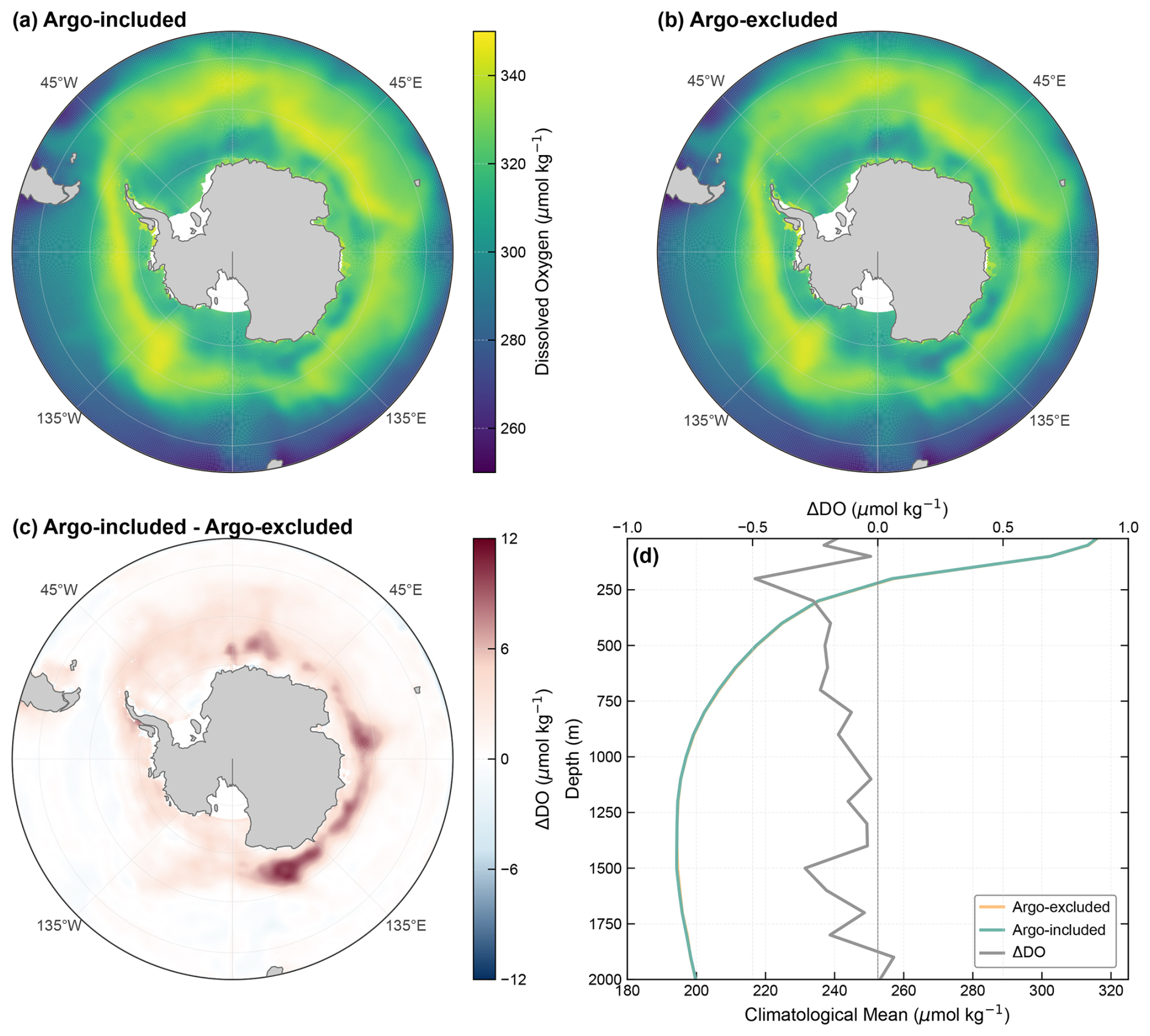
Figure 11 Southern Ocean dissolved oxygen (DO) climatology for 1960–2000. (a) Argo-included climatological mean DO averaged over 1–100 m. (b) Same as (a), but for the Argo-excluded configuration. (c) Difference map (Argo-included minus Argo-excluded) for the 1–100 m climatological mean DO. (d) Area-weighted mean vertical DO profiles south of 45° S from the Argo-included and Argo-excluded reconstructions; the upper x-axis shows the corresponding profile difference (Argo-included minus Argo-excluded).

The results manifest pronounced morphological invariance in the upper-ocean (1–100 m) DO climatology across both configurations. The annular high-oxygen band and its relative position within the circumpolar system remain effectively stationary, implying that Argo inclusion does not induce systematic structural rearrangement. Notably, the difference map reveals localized positive ΔDO hotspots concentrated around the Antarctic margin, with enhanced amplitudes in several coastal/shelf sectors, whereas departures in the open-ocean circumpolar interior are minimal and barely discernible. Consistent with this pattern, the area-weighted mean vertical profiles are nearly overlapping across most depths (panel d), with only a subtle upper-ocean positive offset in the Argo-included configuration that remains below ∼ 0.5 µmol kg⁻¹, indicating modest amplitude refinement rather than depth-dependent reorganization. Collectively, these features suggest that the reconstructed vertical architecture is primarily constrained by consistent physical structure, while the denser modern sampling acts mainly to fine-tune regional magnitudes, thereby supporting the structural integrity of the historical reconstruction.

5.4 Boundary Fusion Effects

While basin-based modeling represents regional environmental heterogeneity, it often induces “step-effect” discontinuities at basin boundaries, resulting in unrealistic shifts in long-term trends and monthly variability at adjacent grid points. To address these boundary artifacts, we implemented a fusion method to smooth inter-basin transitions. We validated this approach by constructing boundary diagnostic samples on a 0.5° by 0.5° grid, specifically selecting adjacent points across basin interfaces.

The diagnostic experiment targeted the 100 m depth layer, a region characterized by high spatial complexity and hydrographic sensitivity. Using a global non-partitioned model as a continuous baseline, we quantified discontinuity magnitudes via the differential trend (Δtrend) and standard deviation (ΔSD) at adjacent cells. Contrasting fused and unfused basin-specific outputs against this reference isolated the consistency gains.

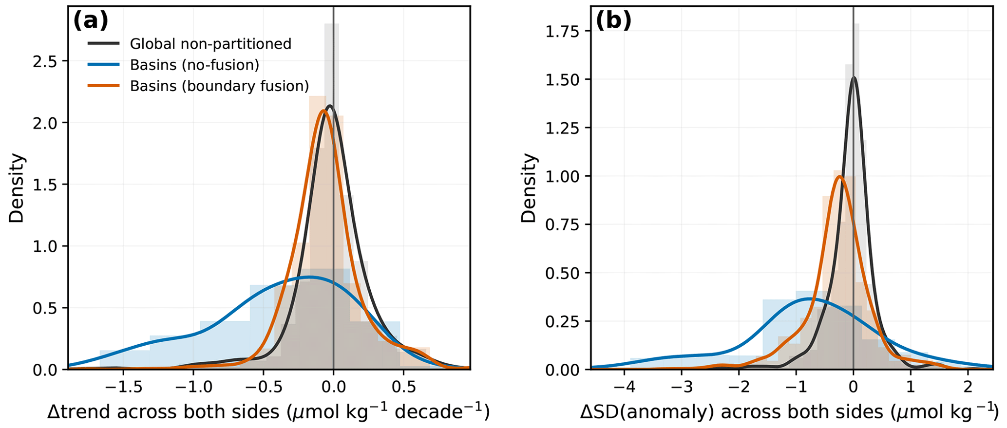
Figure 12 Spatial distribution of the “step-effect” before and after boundary fusion at the 100 m depth layer. (a) Compares the trend differences (Δtrend), and (b) compares the standard deviation differences (ΔSD) across adjacent grid points at the basin boundaries.

Results reveal that the boundary fusion protocol mitigates abrupt statistical shifts, decreasing local biases in the partitioned map (Fig. 12). Improvements in Δtrend and ΔSD demonstrate that the smoothing operator suppresses interface artifacts. Nevertheless, small discrepancies relative to the global non-partitioned baseline persist, indicating that independently trained regional submodels may retain slightly different statistical mappings that are only partially reduced by simple fusion.

Boundary fusion thus serves as an effective strategy for mitigating partition-induced “step-effect” artifacts, yielding a more coherent global spatial structure. While localized gradients remain in high-contrast hydrographic regions, their reduced magnitude indicates a meaningful alleviation of boundary inconsistencies. Future enhancements could involve adaptive fusion schemes or multi-task learning to explicitly share data across regional submodels while preserving specialization.

6 Data availability

The GEOXYGEN dataset produced in this study can be found at https://doi.org/10.5281/zenodo.19703198 (Wang et al., 2026a) and https://doi.org/10.12157/IOCAS.20260223.002 (Wang et al., 2026b). A recommended-use note: because uncertainty in nearshore regions is substantially higher than in the open ocean, coastal and shelf applications should preferentially rely on spatially aggregated and temporally averaged fields rather than on individual native-grid cells.

7 Code availability

The code used to train the models and generate the data product in this paper is openly available from GitHub at https://github.com/layne1202/GEOXYGEN_Code (last access: 24 February 2026) and archived on Zenodo at https://doi.org/10.5281/zenodo.19852901 (Wang, 2026). The repository also documents the key training and evaluation settings (e.g., fixed random seeds) and provides the environment/dependency information needed to reproduce the experiments.

8 Conclusions

By combining multi-source physical and biogeochemical predictors with an adaptive feature-selection strategy, we constructed a hierarchical modeling framework that accounts for underlying biogeochemical controls. Using this framework, we produced GEOXYGEN – a monthly, four-dimensional global ocean dissolved oxygen (DO) product at 0.5° × 0.5° resolution spanning 1960–2024. This product is intended to help address some of the long-standing challenges posed by sparse observations and strong spatiotemporal heterogeneity in historical DO records. Evaluated on an independent out-of-time test composed of withheld years, the reconstruction demonstrates consistently high skill in all depth layers (R²>0.9), confirming its robustness under conservative validation protocols. The resulting high-resolution framework offers superior aggregate fidelity compared to existing 1° products, effectively capturing the fine-scale spatial variance essential for understanding contemporary ocean change. The main strengths of this study are as follows:

Heterogeneity-aware partitioned modeling. By combining vertical stratification with basin provincialization, we train CatBoost regressors within each basin–depth unit. This design directly addresses the limitations of single global ML models, which struggle to represent the spatially varying physical–biogeochemical controls on DO. In combination with adaptive feature selection, inverse-density weighting, year-grouped cross-validation, and cross-boundary fusion, the framework enhances robustness in undersampled regions, minimizes temporal leakage and boundary artefacts, and yields parsimonious, interpretable submodels. The same hierarchical strategy can be readily applied to other biogeochemical tracers or observing systems that exhibit strong regional and vertical heterogeneity.

Adaptive multi-source feature selection. Starting from a rich set of physical, biogeochemical, and spatiotemporal predictors, we employ a two-stage feature-selection procedure within each basin–depth unit to retain only variables that add independent skill. This adaptive, region- and depth-aware integration of multi-source environmental predictors strengthens the representation of upper-ocean processes and water-mass transitions while suppressing noise and redundancy, providing physically interpretable feature sets.

A physically consistent, long-record, high-resolution product. GEOXYGEN delivers global monthly DO fields from 1960 to 2024 on a consistent 0.5° × 0.5° horizontal grid, spanning depths from the surface to 5500 m. Its high performance, climate consistency, and the robustness of the reconstructed trends enable reliable estimates of deoxygenation trends and decadal variations, providing a rigorous benchmark for evaluating and constraining Earth system models.

Nonetheless, GEOXYGEN has limitations related to observational coverage and methodological assumptions. Uncertainty is generally higher in early decades, ice-covered high latitudes, data-sparse deep basins, and nearshore regions. Future work will focus on refining the framework to further reduce uncertainty in these challenging regions and to improve its ability to represent time-varying biogeochemical regimes. Despite these limitations, GEOXYGEN provides a long-term and internally consistent basis for assessing multi-decadal changes in ocean dissolved oxygen. The GEOXYGEN dataset and basin-partition files can be obtained at the following website: https://doi.org/10.12157/IOCAS.20260223.002 (Wang et al., 2026b).