Soil surface change data of high spatio-temporal resolution from the plot to the catchment scale

Although process-based soil erosion models are valuable tools for predicting and managing soil erosion, their limitations arise from constraints in integrating novel data possibilities, uncertainties in parameterisation, and the difficulties in integrating different process scales and their transitions. This study presents a unpresented approach to enhance soil erosion modelling through the utilisation of nested high-resolution spatio-temporal data obtained through structure from motion (SfM) photogrammetry. This technique permits comprehensive observation of soil surface elevation changes during precipitation events, encompassing data acquisition at diverse scales, from plot to slope to micro-catchment. The study presents a unique dataset (Epple et al., 2026, https://doi.org/10.25532/OPARA-1038) that integrates high-resolution time-lapse photogrammetry, field measurements, and UAV (uncrewed aerial vehicle) photogrammetric data, collected over nearly four years. This dataset is intended to enhance the understanding of soil erosion processes and serve as a valuable resource for model evaluation and calibration. The authors encourage the broader scientific community to utilise and expand this dataset, which is expected to contribute to the development of more accurate soil erosion models, thereby improving predictions and management strategies.

1 Introduction

Soil erosion models constitute a valuable resource for stakeholders, policymakers and scientists in the context of soil erosion prediction and decision-making (Batista et al., 2019). From the extensive array of existing models, a variety of models have been developed for diverse scales and for particular process mapping inherent to the scale (Jetten and Favis-Mortlock, 2006). The evaluation of soil erosion models is a complex process, often constrained by the limitations of data availability and the inherent uncertainties in measuring erosion and generating model parameters (Batista et al., 2019; Pandey et al., 2016). The models frequently assume that the input parameters are stationary and that the data pertaining to the surface and soil are unchanging (Jetten and Favis-Mortlock, 2006). Consequently, they encounter difficulties in integrating updated observations that necessitate the consideration of changing model parameters. Furthermore, limitations are evident with regard to cross-scale process understanding and modelling, as well as with respect to the modelled resolution (Epple et al., 2022). A multitude of process-based soil erosion models have been developed for utilisation at field and micro-catchment scales. The smallest of these models use a resolution of 1 m (see, for example, Naranjo et al., 2021), thereby focusing on the dominant processes at these scales (Epple et al., 2022). To guarantee the dependability of the data generated by these models, it is essential to conduct continuous testing and model improvement at all scales (Batista et al., 2019).

The application of photogrammetric methodologies provides a novel opportunity for the evaluation and calibration of process-based soil erosion models. Structure from motion (SfM) photogrammetry, a method for camera-based surface measurements, has previously been employed for comprehensive monitoring of soil surface alterations during an artificial rainfall simulation and a natural thunderstorm event (Eltner et al., 2017). It has been demonstrated that this method is capable of detecting intra-experimental changes in soil surface topography at the micro-scale, due to the near-automatic processing involved (Eltner and Sofia, 2020). The potential for acquiring high-resolution digital elevation models (DEM) at high temporal frequency is made possible by time-lapse photogrammetry, as demonstrated by Jiang et al. (2020) for an artificial slope of 10 m length utilising a DEM acquisition frequency of five minutes. In the field of natural hazards, time-lapse photogrammetry has been employed to achieve cm-accurate estimation of rockfalls at few hourly intervals (Blanch et al., 2024). Observations for soil erosion measurement so far mostly concentrate on single artificial rainfall events, with studies employing rainfall simulations in the laboratory (data acquisition frequency every 30 min, Yang et al., 2021) or in the field (data acquisition before and after the event, Ehrhardt et al., 2022) and do not take higher frequencies into account.

Moving from plot to micro-catchment scale different soil erosion processes are prone to each scale and therefor a range of soil surface change processes are at work, exerting influence over different temporal intervals and spatial scales. These processes result in a continuous transformation of the soil surface. In order to achieve a comprehensive understanding of processes across different scales, we present a new and integrated nested cross-scale data set. This comprises time-lapse photogrammetric plot data, recorded at 10–60 s intervals during artificial rainfall simulations, field data captured on a daily basis, at 0.2 mm intervals during natural rainfall events and via UAV before and after tillage, and UAV data acquired at the catchment scale. The field data were collected over a period of nearly four years. In a recent study, Eltner et al. (2025) demonstrate the value of such data by evaluating the RillGrow (Favis-Mortlock, 2025) soil erosion model with high-resolution observations of rill evolution. Their findings highlight the ongoing challenge of equifinality for process-based soil erosion models and emphasise the need for further model development and data assimilation. They also underscore the potential of spatio-temporal high-resolution data for advancing this field of research. Based on high-resolution DEMs captured at 20 s intervals, Epple et al. (2025) observed soil settling and compaction processes at the onset of rainfall simulations. This provides an empirical approach for differentiating between these processes and erosional processes, thereby enhancing the applicability of photogrammetric data for soil erosion monitoring. It is our intention to make our data available to the soil erosion modelling community for the purposes of evaluation and calibration, as well as further development of soil erosion models, regarding, e.g., cross scale process prediction.

The following section presents the data acquisition structured by the three different scales using SfM photogrammetry. Subsequently, the data were subjected to a preliminary processing stage. The raw data, along with the processed data, are accessible in an open-source format, structured in accordance with the specifications outlined in Sect. 4.

2 Data acquisition

The data were acquired at three different scales (Table 1): by UAV-image capture on micro-catchment scale, single slope scale by event-triggered monitoring posts and on the plot scale via SfM during rainfall simulation.

Table 1 Summary of the observation scales, their time/duration of monitoring, their temporal resolution and size.

Subsequently, the photogrammetric data underwent further processing, resulting in the generation of dense three-dimensional point clouds, which were converted to digital elevation models (DEMs), point precision maps and M3C2 (multiscale model to model cloud comparison) distance measures.

Figure 1 Location of the nested experimental setup in Saxony, Germany (map on the left). The upper row presents a schematic display, while the lower row shows images of the actual setup. From left to right: (a) and (d) illustrate the micro-catchment scale, where SfM (structure from motion) is recorded by UAV (uncrewed aerial vehicle; d = UAV-orthophoto). Panels (b) and (e) present the single slope scale where three monitoring stations were installed, taken daily and event-triggered images for 3D model generation. Nested within the slope scale, (c) and (f) show the plot scale conducting artificial rainfall simulations combined with time-lapse SfM (c is adapted from Schindewolf, 2012).

Figure 2 Image of the nested experimental setup with locations and dates of the artificial rainfall simulations. Image in the lower left corner shows the positioning of the rainfall simulation next to the middle monitoring post on the slope setup.

The nested data acquisition setup was situated in the hilly loess landscape in the vicinity of Nossen in the east of Germany (Fig. 1). The catchment area, which is predominantly utilised for agricultural purposes and covers an area of 5.29 ha, drains to the north into the Freiberger Mulde (see Fig. 1d). The single slope, i.e., field, which is nested in the micro-catchment area, is oriented north-northeast (51°03^′43^′′ N, 13°15^′35^′′ E) and exhibits a gradient of up to 15 %. At the most detailed scale, the plot scale, synthetic rainfall simulations were carried out on 3 m² plots (Fig. 1c, f) situated on the single slope (Fig. 1b, e). The locations of the nested setup are visualised in Fig. 2. Further rainfall simulations were conducted at multiple locations in the east of Germany, across a range of slopes, soil types, soil management practices, soil covers and soil bulk densities (blue flags in Fig. 3). The time frame, as well as soil and surface conditions for the data acquisition process is illustrated in Fig. 3 and can be found in more detail within the published data set.

Figure 3 Timeline of the data collection over almost four years. The nested setup includes the micro-catchment area (depicted in grey), the single slope (shown in green) and the plot with six rainfall simulations (RS) (illustrated in red). The remaining 13 RS (blue boxes) were carried out at different sites. The soil, rain and agricultural conditions, sampled and observed in the field and in the laboratory, are summarised in the dashed boxes. The magnitude of the observed scales is highlighted in each row. The following abbreviations are used: UAV = uncrewed aerial vehicle, SfM = structure from motion.

2.1 Catchment scale

At the micro-catchment scale, an orthophoto and a DEM were calculated via UAV-photogrammetry for the 22 July 2020 (Fig. 1d). The image data was acquired using a DJI Phantom 4 RTK UAV considering a standard photogrammetric flight pattern (85 % and 70 % forward and strip overlap, respectively). RTK was not enabled and we solely relied on GCPs, distributed around the catchment and measured with RTK-GNSS, for georeferencing. Further image data of the micro-catchment was taken on nine days between April 2020 and September 2022, these are available in unprocessed form. The observation height was generally set to a range of 30–50 m, with nadir images resulting in a ground sampling distance of 2 cm. The data thus provides the basis for testing soil erosion models at the catchment scale and enabling modeller the upscaling of slope scale parametrisation to the catchment scale. Therefore, the objective is not to calibrate a model, but rather to serve as a high-resolution model input and for model testing. Furthermore, while this dataset is focused on the micro-catchment scale, it also provides a critical high-resolution benchmark for broader-scale erosion assessments. At coarser spatial resolutions (relying on aerial- or satellite-based data), models need to simplify, e.g., surface connectivity features (such as roughness) or overlook small-scale erosion features like rills. This high-resolution GSD allows for the validation of sub-grid parameterizations in regional models, bridging the gap between localized physical processes and large-scale sediment yield estimations (Panagos et al., 2015; Borrelli et al., 2021).

2.2 Single slope scale

The single slope (see Table 1 for dimensions and Grothum et al., 2025 for more detail), was situated within the micro-catchment area and maintained in a clear state, with vegetation removed by means of cultivating downslope at a depth of 10 cm at three-to-six-week intervals. It was monitored over a period of almost 3.5 years (July 2020 to April 2024) by a total of 15 cameras mounted on three monitoring stations. Five event-triggered and synchronised RGB cameras were installed on each monitoring device, fixed on a traverse in 4 m height), along with an Arduino-based control station connected to a rain gauge, taking pictures every 0.2 mm of rainfall (controlled by a tipping bucket). Furthermore, the cameras were triggered at 10:00 a.m. CET daily (controlled by an RTC – real time clock). The areas observed by the monitoring stations, which were 4 m wide and 7.5 m long (marked in yellow in Fig. 4a, d), were situated within the central portion of the field, which was cultivated in three parallel lines along the slope. The area was delineated by ground control points (GCPs) on the left and right sides. The number of individual cameras and their positions are illustrated in Fig. 4a up until July 2022 and modified for the period after July 2022 in Fig. 4d. The modification, initiated due to storm damage, involved the rotation of two monitoring posts and their repositioning to face downwards, thereby facilitating the capture of the bottom of the slope more effectively and reducing the amount of rain droplets blown onto the camera lenses. A comprehensive description of this structure can be found by Grothum et al. (2025). In addition to the spatio-temporal high-resolution, event-triggered data acquisition at three positions (upper, middle, and lower slope) (Fig. 4), UAV-SfM data were collected over the entire slope before and after both rainfall events and tillage.

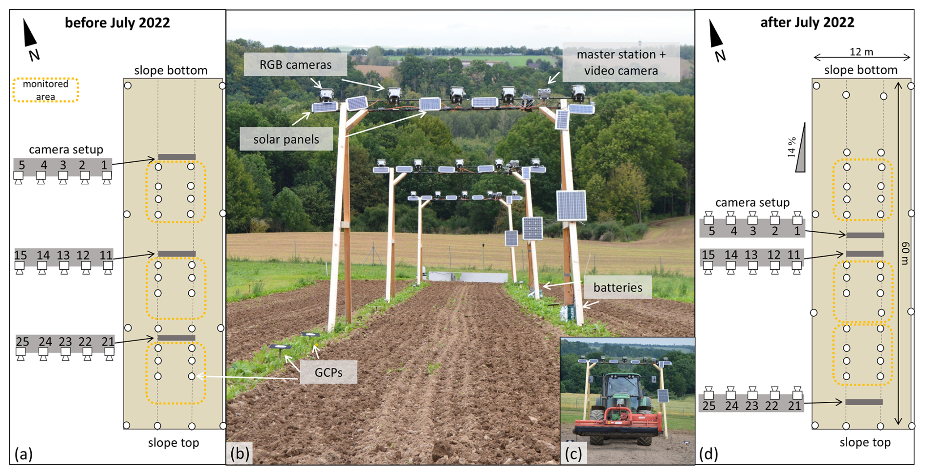
Figure 4 Monitoring setup on the slope scale with three monitoring stations, each equipped with five RGB cameras (b). The schematic representation in (a) and (d) includes the camera designations and positions of the GCPs (ground control points). Panel (a) presents the setup employed until July 2022. Subsequently a slight modification was implemented as shown in (d). The height of the posts was chosen to facilitate the mechanical removal of vegetation (c) while minimising potential restrictions.

2.3 Plot scale

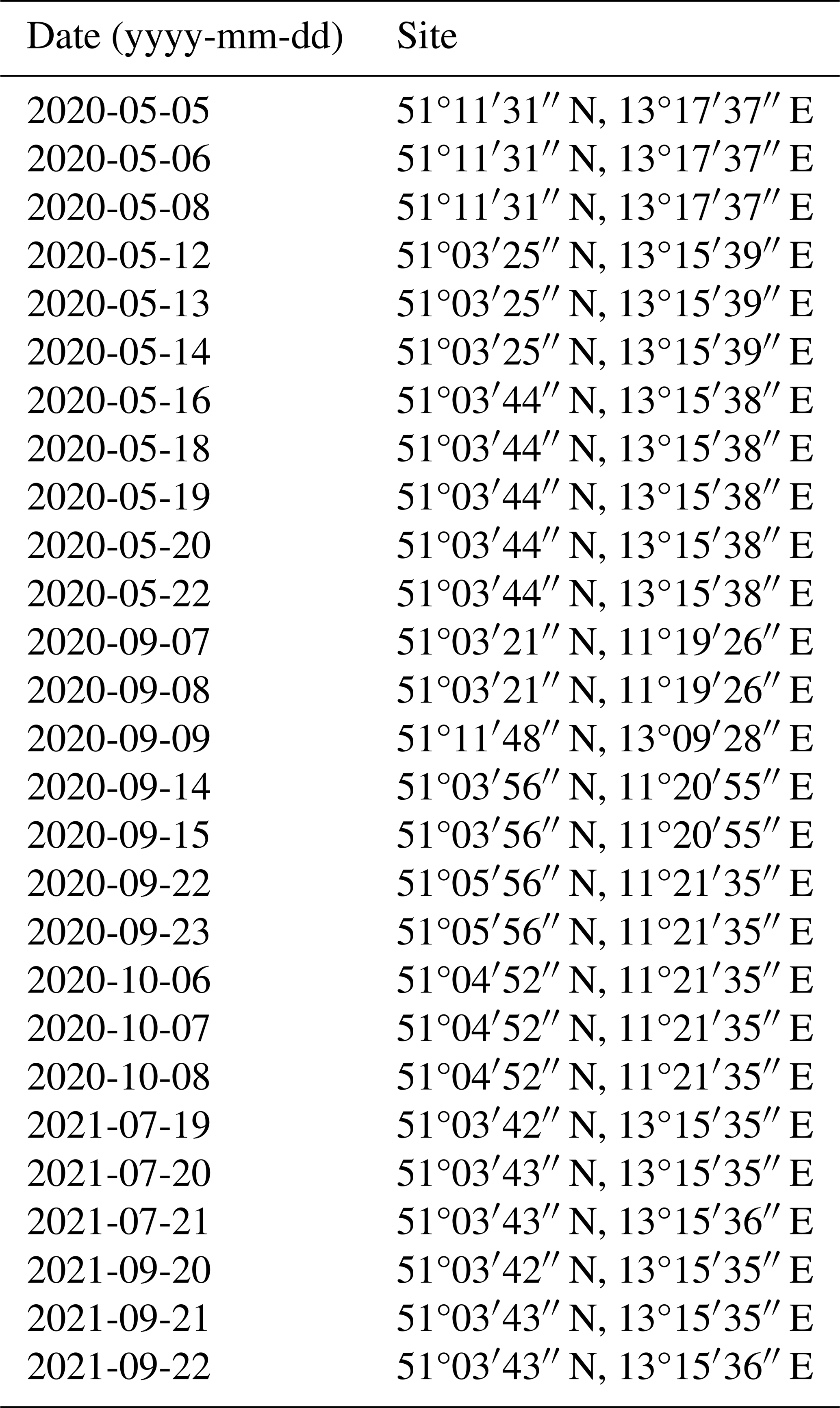
Six rainfall simulations were performed at the plot scale; encompassing the lower, middle and upper regions of the monitored slope in July and September 2021 (Fig. 3). Furthermore, a total of 13 additional rainfall simulations were carried out at sites in Saxony and Thuringia between May and October 2020 (Table 2).

Table 2 Coordinates of the different rainfall simulations in Thuringia and Saxony, Germany.

More information on each individual plot can be found in an overview table as part of the data publication this article accompanies. GCPs were installed around each plot, driven at least 10 cm into the ground, in order to enable georeferencing and ensure stability during the experiment. The rainfall simulator used is described in detail in Schindewolf and Schmidt (2012). The precipitation is dispersed onto the ground from three rain hoods with oscillating nozzles at an elevation of 2 m. The velocity, distribution and size of the raindrops produced by the VeeJet 80/100 nozzles are comparable to those of a heavy rainfall event (Kainz et al., 1992). At the base of the plot, which was enclosed by metal sheets and had a length of 3 m and a width of 1 m, a sediment collector was used to facilitate the collection and measurement of runoff and sediment concentration (see also Table 3). At the outset of the rainfall simulation, the intensity of the precipitation was gauged by enclosing the plot with a protective sheet and measuring the total discharge. Thereafter, the infiltration experiment started (Fig. 5, A in timeline). Once a steady state of infiltration had been reached, the apparatus designed to simulate slope lengths exceeding 3 m was activated. The runoff experiment (Fig. 5, B in timeline) was conducted for a further 10 to 14 min. Subsequently, the water supply feeding surface runoff and rainfall was terminated for approximately one hour, after which the repetition was carried out. An individual camera setup on posts at heights of 1.5 to 3 m, comprising eight to eleven synchronised digital single-lens reflex (SLR) cameras (schematic in Fig. 5), captured images to generate DEMs at 10, 20 and 60 s intervals (A – runoff experiment, B – infiltration experiment, and break, referring to the camera symbols in the timeline in Fig. 5). Exceptions are the rainfall simulations carried out in September and October 2020. These were performed with a minor alteration, the first infiltration experiment was directly followed by a break before the second infiltration experiment took place, followed by a runoff experiment (corresponding to Fig. 5, the timeline for these simulations can be described as A-break-A-B). As an addition to the camera monitoring system, a camera was utilised for all-round SfM data capture during the break and before and after the experiment. This was done in order to generate 3D models with Agisoft Metashape (v.1.8.3) images acquired from the most suitable perspectives, with the aim of avoiding data gaps due to occlusions as much as possible. This offers a more complete model with a higher point density compared to the synchronised camera setup resulting in a valuable data set for model input.

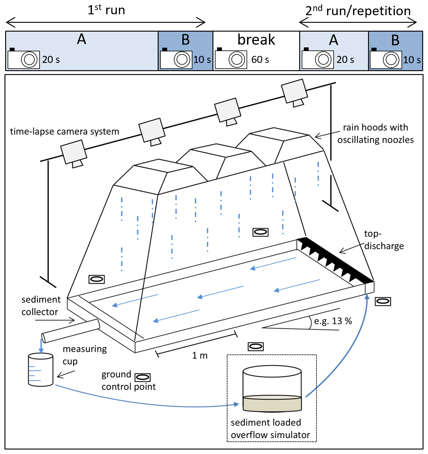
Figure 5 Schematic representation of an artificial rainfall simulation, as adapted from Schindewolf (2012) and monitored by a synchronised time-lapse camera system. The blue boxes at the top show the timeline of a rainfall simulation (1st run and 2nd run/repetition). Each run consists of an infiltration experiment (A) and a runoff experiment (B), separated by one-hour interval of no rainfall. The cameras indicate the frequency of the SfM (structure from motion) image taking, between every 10–60 s.

Soil samples were collected in the immediate vicinity of the plot at three distinct time points: prior to the experiment/before 1st run A (six core samples), during the experimental break (three core samples) and after the end of the experiment/after 2nd run B (three core samples). The core samples were weighed in the laboratory both before and after drying, thus providing data on the bulk density and soil moisture content of the topsoil. The restricted spatial distribution and limited number of samples were a consequence of the lack of available space. Particle size distribution data were obtained using ultrasonic dispersion and Köhn sieve sedimentation techniques, applied to a subset of soil samples. The total organic carbon (TOC) was analysed using an elemental analyser coupled with isotope ratio mass spectrometry (EA-IRMS). The extent of surface vegetation and stones was estimated as a percentage, and the slope was measured. Figure 3 presents a summary of the data pertaining to soil, surface, rainfall and tillage conditions within the blue dashed box.

3 Data processing and results

Figure 6 shows the complete data processing workflow. Prior to data collection, all cameras used in terrestrial applications at the single slope and plots were pre-calibrated using a temporary calibration field (e.g., Eltner and James, 2022). The coordinates of the markers were determined with a mm-precision using a folding rule. The objective of the camera calibration was to ensure the precise modelling of the ray path from the object point through the camera's projection centre to the image sensor.

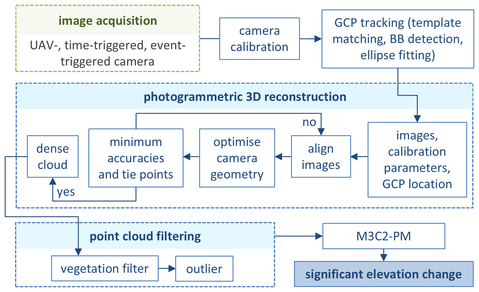
Figure 6 Image processing workflow adapted after Epple et al. (2025) (GCP = ground control point, M3C2 PM = Multiscale Model to Model Cloud Comparison with Precision Maps, BB detection = bounding box detection).

All cameras were synchronised during data capture using a wired connection between the cameras, thereby enabling simultaneous triggering. At the plot scale image matching went well during the experiments lasting between 30 to 120 min. Due to the occurrence of clock drifts and trigger failures in the cameras over the four-year measurement period at the field scale, an automatic time-matching approach was developed (Grothum et al., 2025). In order to orient the image measurements and the resulting 3D models in a scaled reference frame, GCPs were utilised at the plot, slope and micro-catchment setups. A Leica TCRM 1102 total station, which can measure points with mm accuracy, was applied to map the GCP coordinates at the single slope and micro-catchment. During the rainfall simulation, the GCPs were either measured by the same total station or using a tape measure between the GCPs in combination with photogrammetric adjustment (as done in Eltner et al., 2017) to get mm-accurate coordinates. The GCPs were automatically mapped in the images using a template matching approach based on normalized cross-correlation at the plots. At the field scale, a deep learning-based approach for bounding box detection was used, which demonstrated greater robustness throughout the year (Blanch et al., 2025). At the field scale, the coordinates of the GCPs were refined to sub-pixel accuracy through the application of ellipse-fitting (Grothum et al., 2025). A more detailed description of the technical procedure can be found in Grothum et al. (2025).

The external (camera poses, i.e., orientations and positions) and internal (only focal length and principle point) camera geometry were estimated within a bundle adjustment (using Agisoft Metashape) considering the pre-calibrated camera parameters, the GCPs and the tie points found via image matching. Furthermore, the precision of the tie points was estimated by the M3C2-PM (multiscale model to model cloud comparison with precision maps) method (James et al., 2017). The adjustment was performed in an iterative manner, changing input parameters, such as number of required image point matches, if the overall accuracy was not sufficient. After image alignment and adjustment, a multi-view stereo (MVS) matching process was used to calculate the dense point clouds. Subsequently, the dense point clouds were subjected to filtering in order to remove any outliers and vegetation that may have been present (Grothum et al., 2023).

The point precisions of tie points were interpolated to the dense point cloud, thus enabling the subsequent derivation of a spatially distributed level of detection during change detection, i.e., point cloud differencing with the M3C2 approach (Lague et al., 2013). Each time series point cloud was compared with the initial point cloud in the series. A more detailed account of the whole data processing can be found in Grothum et al. (2025).

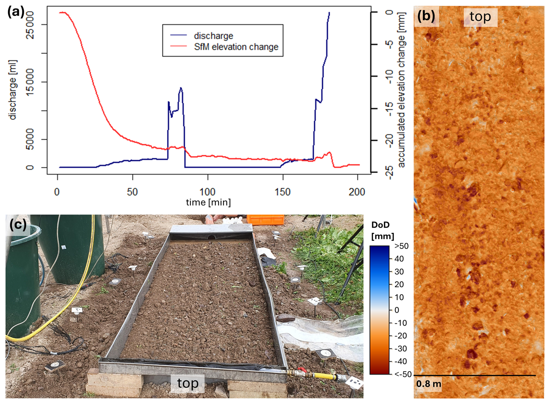
Figure 7 Rainfall simulation results on 21 July 2021 on the plot scale. (a) Timeline of the accumulated spatial averaged elevation change measured via SfM (structure from motion) and the measured discharge at the plot's outlet covering the whole simulation time. (b) DoD (digital elevation model of difference) subtracting the dense clouds captured before and after the rainfall simulation presenting the spatially distributed elevation change. (c) Image of the rainfall simulation plot, shortly after the start.

Figure 7 presents the evaluation of data collected during the rainfall simulation 21 July 2021. The soil had been freshly cultivated just two days prior, resulting in a loose and unconsolidated topsoil. As a result, a pronounced elevation decrease was observed at the beginning of the event (Fig. 7a), reflecting a combination of erosional and predominantly non-erosional processes such as compaction and consolidation. Epple et al. (2025), consider ten rainfall simulations of this dataset and provide on that base a detailed discussion of these initial elevation changes under varying soil conditions. In this context they introduce an empirical method to distinguish non-erosional from erosional processes. The DEM of Difference (DoD) illustrates widespread surface lowering across the plot, with localized elevation losses exceeding 5 cm. These pronounced changes are attributed primarily to aggregate breakdown and other highly localized processes.

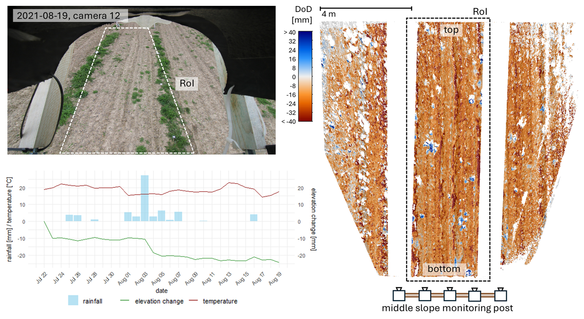
Figure 8 Results of a 28 d observation time at the middle slope position in July and August 2021. At the top: image of the camera 12, taken on 19 August 2021 at 10:00 a.m. At the bottom: timeline for the period 22 July 2021 (right after tillage) until 19 August 2021 (day before tillage), with the average M3C2 elevation change, the temperature and the daily rainfall. To the right: DoD (digital elevation model of difference) subtracting the days 22 July and 19 August 2021, with the schematic illustration of the middle slope monitoring post (bottom), cameras facing upslope. The RoI (region of interest) is marked by the dotted black/white box.

Figure 8 shows exemplary results on the slope scale, visualising the changes in elevation during a 28 d observation period on the middle slope position in July and August 2021. Strongest elevation decreases were measured right after tillage on 23 July and as a result of heavy rainfall on 3 August (Fig. 8, timeline). The DoD illustrates strongest elevation decreases along the tillage lines, the predominant flow paths, which lead to rill erosion. Elevation increases (blue patterns in the DoD) are a result of vegetation growth, as can be seen in the image at the top.

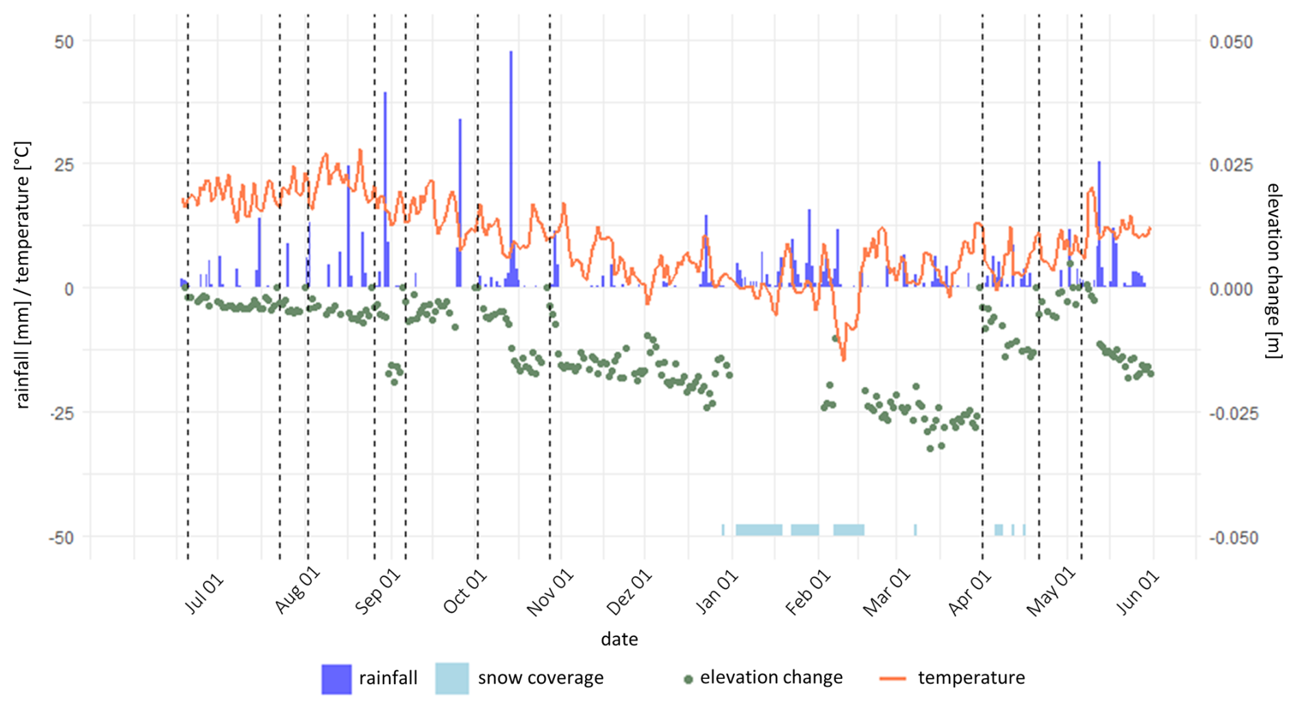
Figure 9 Timeline presenting the averaged M3C2 elevation change development over the year June 2020 until June 2021 measured by the middle slope monitoring post (dotted vertical lines indicate tillage and therefore an elevation reset).

In addition to the information on single rainfall simulations and a month of rainfall events, the data offer information on a yearly scale. Figure 9 presents 12 months of elevation change in 2020–2021 recorded at the middle slope position. With no tillage and therefore no reset from Novembre 2020 until April 2021, information about the seasonal development during the winter months can be derived. Small rainfall events, snow coverage and snow melting lead to an average decrease of 3 cm during these months. As already presented in Fig. 7 the data show high potential for consolidation and compaction on the site right after tillage. At this time, already small rainfall events can lead to comparable high elevation decreases (e.g., October 2020).

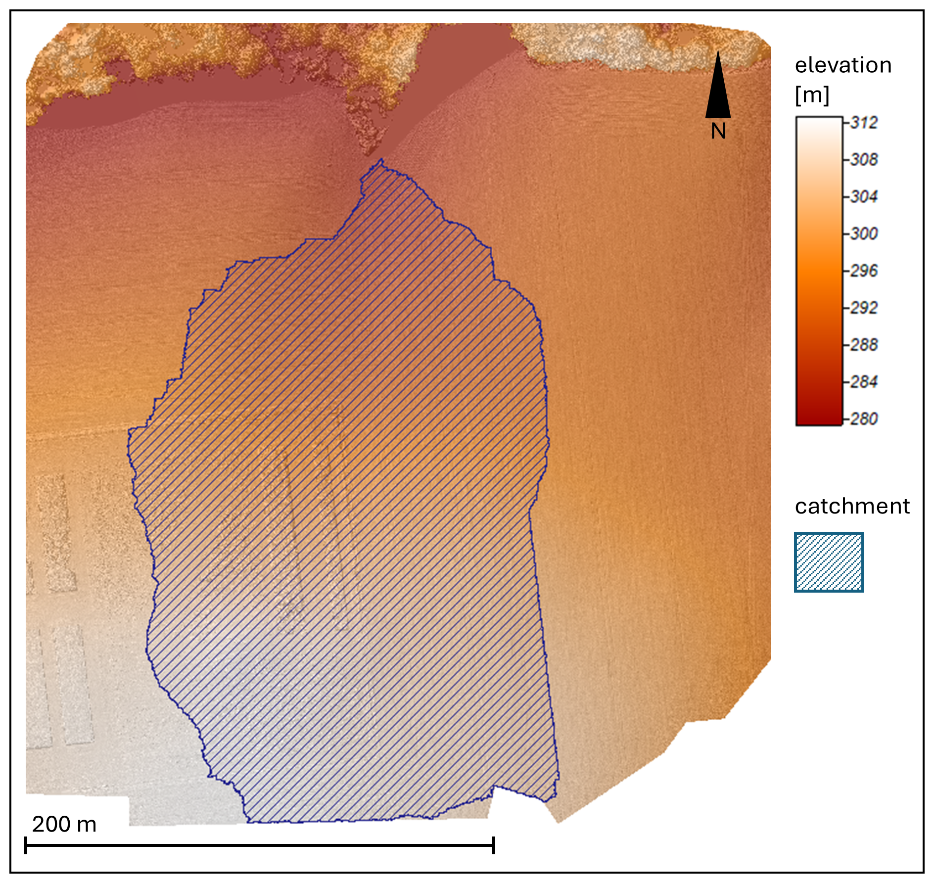
Figure 10 DEM (digital elevation model) of the micro-catchment scale (22 July 2020), with the micro-catchment marked in blue, visualised with an analytic hillshade in the back.

Figure 10 presents the information, available on the micro-catchment scale. Both the slope as well as ten of the plot positions are nested within this blue area. This dataset as well as the UAV-images of eight further flights during the monitoring period are an important part of this nested experimental setup. It serves on the one hand as model input for soil erosion modelling at the micro-catchment scale and provides on the other hand a data base for upscaling approaches, offering processed-based soil erosion modelling, the opportunity to test the plot-calibrated and slope-validated information on the next scale.

4 Structure of the data archive

The dataset is structured according to the three scales: plot, slope and micro-catchment (Fig. 11). Each observation scale is divided into two datasets: a raw and a processed one. The raw dataset comprises the unprocessed images (from the terrestrial used SLR and the UAV cameras), 3D coordinates of the GCPs (i.e., in object space) and empirical field data (rainfall simulation results, soil data, meteorological data, etc.). The processed data set includes the camera calibration protocols, the reconstructed dense point clouds, the orthophotos, the point precision maps and the M3C2 distances per point. Please find a detailed overview of the data in the data description accompanying the data.

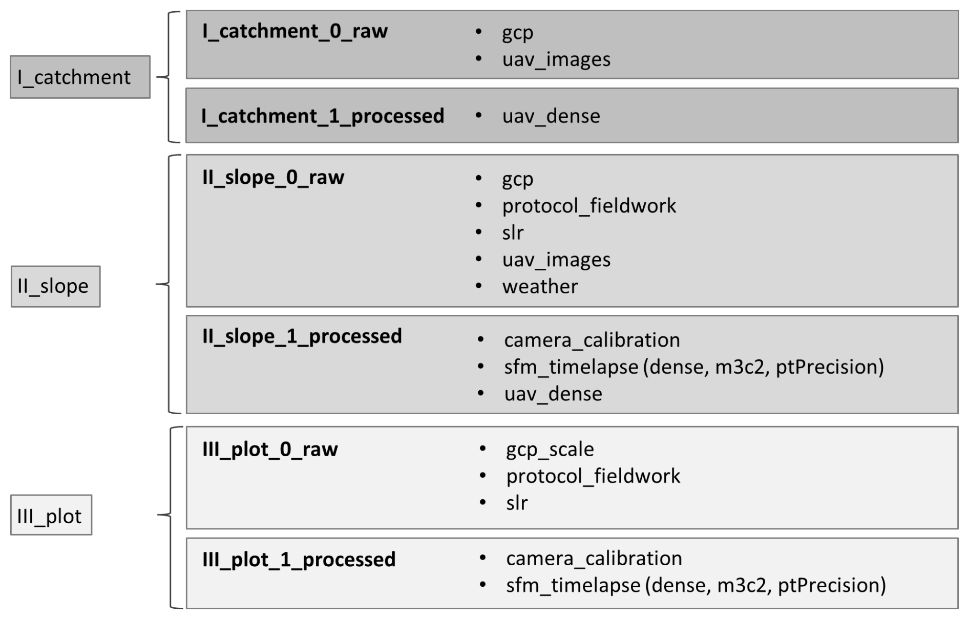
Figure 11 Dataset structured by the observation scales and further subdivided into raw and processed data. (gcp = ground control point, slr = single lens reflex, uav = uncrewed aerial vehicle, sfm = structure from motion, ptPrecision = point precision map; lowercases used as in the data archive).

5 Data quality

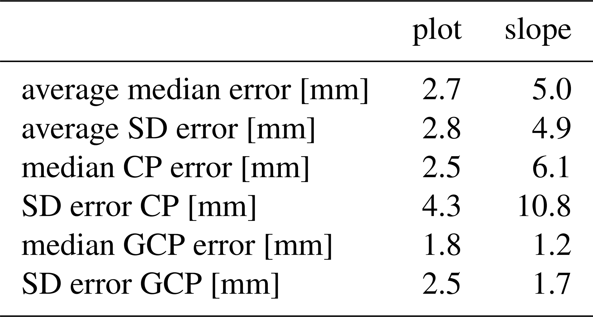
An overview of the accuracies can be found in Table 3. The point precision files (ptPrecision) in the “time_lapse” folders within the dataset offer mm-precisions on every connection point in every 3D-model on both plot and slope scale, averaged by the “average median error”. Information on the RMSE (root mean square error) at the GCPs and CPs for every 3D-model are included as log-files in the “time_lapse” folder.

Table 3 Average accuracy metrics of the plot and slope data, excluding strong outliers. CP and GCP refer to check point and ground control point respectively, SD stands for standard deviation.

6 Data availability

The described data set can be found by the following DOI: https://doi.org/10.25532/OPARA-1038 (Epple et al., 2026).

7 Code availability

The code for photogrammetric time-lapse data processing has been published by Grothum et al. (2025, https://doi.org/10.5194/soil-11-1007-2025).

8 Recommendations and conclusions

We introduce a novel nested dataset designed for the detection and analysis of soil surface changes, which we make available to the broader scientific community. This dataset provides high-resolution spatio-temporal data on geomorphological processes, including erosion triggered by heavy rainfall and seasonal elevation changes. It spans a range of spatial scales, from 3 m² to 5 ha, and includes variable data acquisition frequencies, offering a distinctive resource for in-depth examination of soil dynamics. To ensure maximal transparency, we provide both the raw data required to construct DEMs and pre-processed dense point clouds for further use. While the current dataset is based on a loess site in eastern Germany with a limited slope range and moderate rainfall events, we encourage researchers to expand its scope. This can be achieved by integrating camera systems during rainfall simulations and collecting high-resolution spatial and temporal data during natural rainfall events. For this purpose, both software and hardware are made openly accessible and adaptable to other locations and conditions. Such contributions will enable to address existing challenges in soil erosion modelling by providing new observations for model evaluation and calibration. Furthermore, this unique dataset offers a first-of-its-kind opportunity to train artificial intelligence (AI) models and compare their performance with conventional process-based soil erosion models. We anticipate that this dataset will significantly enhance the understanding of soil erosion processes and contribute to the development of more accurate and robust predictive models.