The newly developed Multi-ensemble Biomass-burning Emissions Inventory (MBEI): characterizing and unraveling spatiotemporal uncertainty in global biomass burning emissions

Large discrepancies among existing inventories hinder a consensus on the true magnitude and long-term trends of global biomass burning emissions. To address this, we developed the Multi-ensemble Biomass-burning Emissions Inventory (MBEI), a framework integrating bottom-up and top-down approaches with multi-source data to generate eight sub-inventories for the period 2003–2023. This ensemble approach allows for the explicit quantification of emission uncertainty at a 0.1° grid scale. We estimate global annual CO₂ emissions at 7304 (4400–9657) Tg, with the maximum estimate exceeding the minimum by over two-fold. The uncertainty exhibits significant spatial heterogeneity: it is highest in low-emission regions like Australia and the Middle East (6.0–7.0 fold difference), whereas traditional hotspots like Africa show lower divergence (Approximately 2 fold). Temporally, a distinct decadal shift was identified: global emissions declined from 2003 to 2013 due to reduced tropical burning, but reversed to an increasing trend from 2013 to 2023, driven by intensified fires in northern high-latitudes and extreme events. Comparisons confirm that the MBEI mean provides a robust central estimate, while its max-min range effectively encompasses other major inventories. By providing explicit uncertainty bounds, MBEI enhances the reliability of atmospheric modeling and climate assessments. The dataset is publicly available at https://doi.org/10.5281/zenodo.18104830 (Liu and Yin, 2025).

1 Introduction

Biomass burning, encompassing forest fires, grassland fires, and the burning of agricultural residues, is a key disturbance in terrestrial ecosystems (Bowman et al., 2020; Jones et al., 2022). It profoundly influences local and global ecological processes and climate systems by releasing large quantities of greenhouse gases (GHGs) and aerosol particles (Bowman et al., 2009; Letu et al., 2023; Pellegrini et al., 2018; Shi et al., 2025; Yin, 2021). Accelerating climate change is driving significant shifts in the spatiotemporal patterns of global biomass burning, affecting its frequency, intensity, and duration. Observational data indicate that the incidence of extreme biomass burning events has increased 2.2-fold in the last two decades (Cunningham et al., 2024; Wang et al., 2023), and climate models project that high-risk areas for global biomass burning will expand by nearly one-third by the end of the 21st century (Senande-Rivera et al., 2022). Notably, while the burned area is shrinking in some traditional high-frequency burning regions (e.g., tropical rainforests) (Andela et al., 2017; Zheng et al., 2021), the fire-prone season is substantially extending. In regions such as southeastern Australia, eastern Siberia, and eastern North America, the length of fire weather season has increased by 27 %–94 %, significantly prolonging the period during which ecosystems are exposed to fire risk (Jones et al., 2022).

The increase of biomass burning frequency is raising atmospheric concentrations of GHGs, thereby exerting a strong perturbation on Earth's biospheric processes (Andreae, 2019; Andreae and Merlet, 2001; Yin et al., 2025). Between 1997 and 2016, global carbon emissions from biomass burning averaged 2.2 Pg C per year, equivalent to approximately 6 % of global fossil fuel CO₂ emissions in 2014 (Friedlingstein et al., 2025; Liu et al., 2024; van der Werf et al., 2017). This increase in GHGs intensifies global warming, creating a feedback loop that is projected to elevate the risk of extreme fire weather by at least 50 % in key regions such as western North America, equatorial Africa, Southeast Asia, and Australia by 2080 (Touma et al., 2021). Furthermore, particulate matter (e.g., black carbon, brown carbon, and organic carbon) emitted from biomass burning poses a serious threat to human health (Reid et al., 2005; Zhang et al., 2020). A meta-analysis of 81 studies (1980–2020) (Karanasiou et al., 2021). showed that exposure to PM_2.5 and PM₁₀ from biomass burning is significantly associated with all-cause mortality, corresponding to a 1.31 % (95 % CI: 0.71–1.71) and 1.92 % (95 % CI: 1.19–5.03) increase for every 10 µg m⁻³ rise in PM₁₀ and PM_2.5. These effect sizes exceed typical estimates for all-source ambient particulate matter, indicating that biomass burning PM may pose greater health risks than general ambient PM. From 1990 to 2019, PM_2.5-related excess mortality in equatorial Asia increased threefold, with approximately 317 thousand of these deaths attributed to high-intensity biomass burning from Indonesian peatlands (Yin, 2023).

Establishing high-precision emission inventories is crucial for assessing the impacts of biomass burning on the global atmospheric environment and public health (Bray et al., 2021; Filonchyk et al., 2024; Ramanathan and Carmichael, 2008). Trace gases and aerosols released by biomass burning not only affect global climate but also alter regional atmospheric chemistry via transboundary transport (Andreae, 2019). Atmospheric Chemistry Transport Models, which are used for air quality forecasting and source apportionment, rely on emission inventories with high spatiotemporal resolution and reliability. Such data are crucial for accurately resolving pollutant transport and transformation pathways, as well as for quantifying their contributions to pollution (Matthias et al., 2018; Wang et al., 2014). Currently, the construction of global and regional biomass burning emission inventories primarily relies on two established estimation pathways, the bottom-up and top-down approach. The bottom-up approach typically estimates emissions based on satellite-derived burned area (e.g., MODIS MCD64A1) combined with fuel load, combustion completeness, and emission factors (van der Werf et al., 2017; Wiedinmyer et al., 2023). The typical inventories of this approach include the Global Fire Emissions Database (GFED) and the Fire INventory from NCAR (FINN) (Giglio et al., 2006). In contrast, the alternative top-down approach estimates emissions based on Fire Radiative Power (FRP) retrieved from satellites in thermal infrared bands. This method utilizes the relationship between the time-integrated FRP, known as Fire Radiative Energy (FRE), and the total dry matter consumed, a relationship often calibrated using field observations (Ichoku and Ellison, 2014; Wooster et al., 2005). It estimates emissions by fitting the combustion curve of dry matter consumption derived from satellite-retrieved FRP (Santoro, 2018). The typical inventories include the Global Fire Assimilation System (GFAS) and the Quick Fire Emissions Dataset (QFED) (Andela et al., 2015; Giglio et al., 2020).

Although these two methods provide clear theoretical frameworks, their practical implementation varies among researchers in their choice of data sources, parameters, and algorithmic details, leading to significant discrepancies in the resulting inventories (Hoelzemann et al., 2004; Ichoku and Kaufman, 2005; Ito and Penner, 2004; Zhang et al., 2014). Consequently, estimates of total emissions for the same region or period can differ considerably (N'Datchoh et al., 2025; Pereira et al., 2016; Shi and Matsunaga, 2017; Whitburn et al., 2015). This discrepancy poses a key challenge in the field, as it not only directly impacts the accuracy of atmospheric chemistry simulations and climate effect assessments (Liu et al., 2020; Longo et al., 2010; Stroppiana et al., 2010; Williams et al., 2012) but also leads to a lack of clear consensus on the true magnitude and long-term trends of global biomass burning emissions.

A growing body of evidence suggests that under the dual threats of climate change and human activities, the spatial distribution of global biomass burning is undergoing significant shifts. Fire activity is weakening in some traditional tropical hotspots (e.g., African savannas) while intensifying in high-latitude boreal forests (Tyukavina et al., 2022; van Wees et al., 2021; Yin et al., 2020b; Zheng et al., 2021, 2023). These complex and opposing regional trends obscure the long-term trajectory of global total emissions. In this context, the limitation of emission inventories, which provide only a single estimate, becomes more prominent. A single value cannot capture the extent to which observed regional trends reflect genuine physical processes versus mere algorithmic artifacts of a particular inventory. Therefore, accurately assessing the current state of biomass burning emissions requires not only improving the precision of inventories but also developing new methods to systematically quantify their uncertainty.

To address this challenge, we constructed the Multi-ensemble Biomass-burning Emissions Inventory (MBEI), a global biomass burning emission dataset for 2003–2023, by integrating mainstream top-down and bottom-up algorithms. This ensemble approach incorporates two fire-detection products and four sets of key input variables, resulting in eight distinct sub-inventories that quantify emissions for 11 key species (e.g., CO₂, PM_2.5, BC, and NO₂). By analyzing the mean and the maximum-minimum range (hereafter referred to as the “Max–Min band”) of these eight sub-inventories, our study provides a new quantitative estimate of global biomass burning emissions over the past 21 years and, crucially, reveals their uncertainty across various spatial scales. It offers quantitative evidence to better interpret the shifts in global biomass burning patterns. The advantages of this new inventory allow data users (such as atmospheric chemistry modelers and climate assessment experts) to directly incorporate the variability of emission estimates into their analytical frameworks, thereby providing critical data support for dissecting complex global biomass burning dynamics and enhancing the robustness of their assessment results.

2 Materials and Methods

2.1 Datasets

The MBEI integrates two established methodologies: a bottom-up approach based on burned area and a top-down approach based on FRP (Vermote et al., 2009; Wiedinmyer et al., 2006). Active fire detections were sourced from the MODIS Near-Real-Time product (MCD14DL). To assess uncertainty stemming from detection confidence, we created two parallel processing streams using fire pixels from both Aqua and Terra satellites (2003–2023): one including all detected fires, and another restricted to fires with medium-to-high confidence (> 30 %). In addition, we introduced combination in key input variables: the bottom-up algorithm was driven by two alternative aboveground biomass (AGB) datasets (Biomass_cci and GlobBiomass), while the top-down algorithm utilized two different biome maps (8-class and 30-class) to define emission coefficients. For consistency, all input datasets were resampled to a common 0.1° spatial resolution and monthly temporal resolution. A comprehensive list of the datasets used in this study is provided in Table 1.

Table 1 Datasets used in this study.

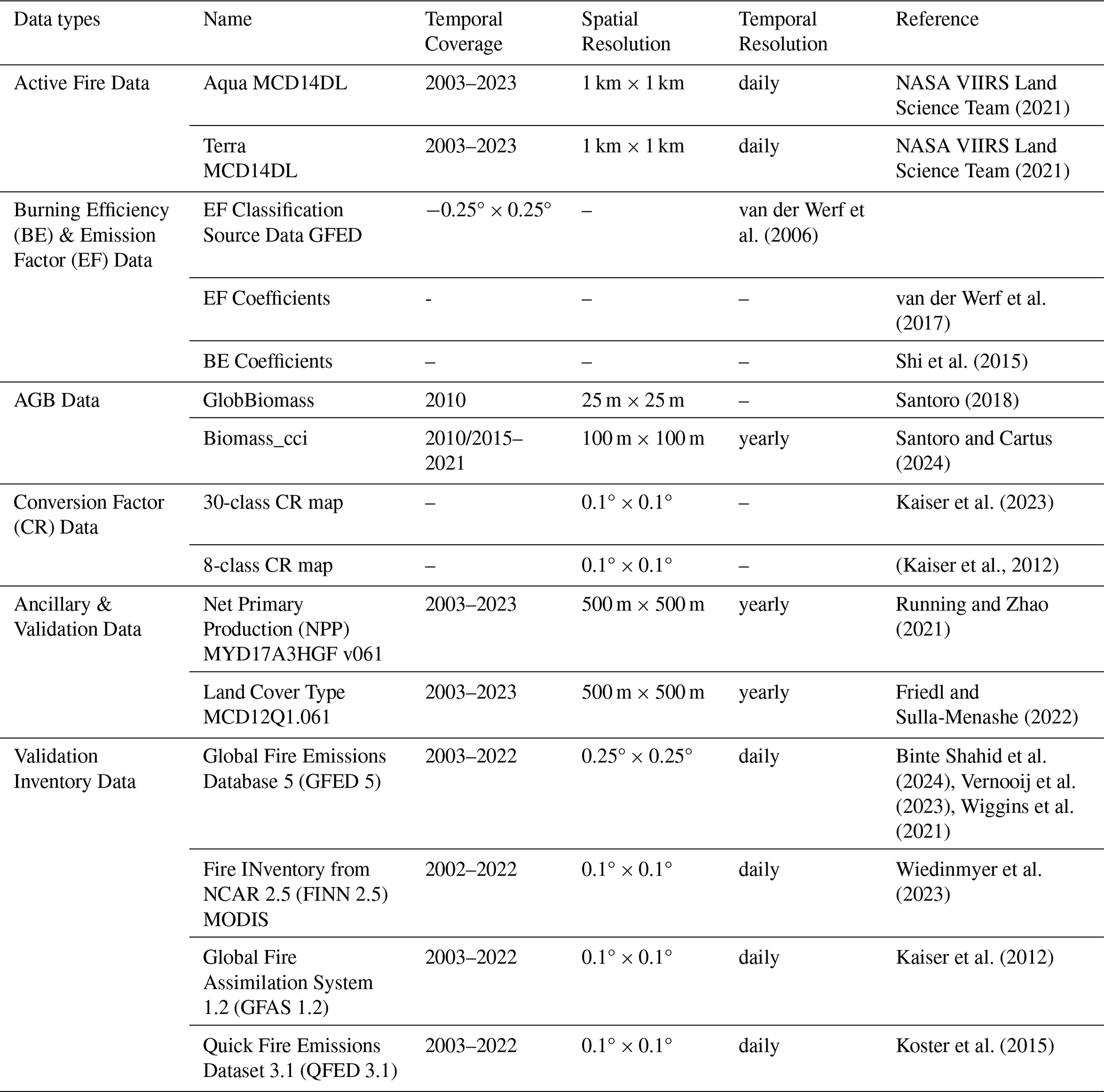
Note: The 8-class biome map is derived from the 30-class biome map. See Fig. S1 in the Supplement for its spatial distribution.

2.1.1 Active fire detection and fire radiative power

The sourced active fire data were obtained from the MODIS Near-Real-Time active fire product (MCD14DL C6.1), provided by NASA's Fire Information for Resource Management System (FIRMS). This product provides fire detections from both the Terra and Aqua satellites based on the MOD14/MYD14 thermal anomalies algorithm (Giglio et al., 2006). Each active fire detection represents the center of a 1 km pixel flagged as containing one or more fires.

For the period 2003–2023, we extracted daily fire locations, detection confidence, and FRP values. These 1 km daily data were then aggregated into monthly 0.1° grids, which form the primary input for both our top-down and bottom-up frameworks.

2.1.2 Burning efficiency and emission factor

To assign region- and vegetation-specific BE and EF, we first utilized the annual 500 m MODIS Land Cover Type product (MCD12Q1 C6.1), adopting its International Geosphere-Biosphere Programme (IGBP) classification scheme. We then assigned a BE value to each of the 17 IGBP classes using coefficients derived from Mieville et al. (2010) and Shi et al. (2015), with the specific values detailed in Table S3.

Emission factors were assigned by intersecting the MCD12Q1 land cover map with the 14 continental-scale regions defined by GFED (van der Werf et al., 2017). This process yielded a unique EF for each landcover region combination, allowing us to estimate emissions for 11 key atmospheric emission species as detailed in Table S4.

2.1.3 Aboveground biomass

To quantify available fuel load for the bottom-up framework and assess related uncertainties, we employed two independent global AGB datasets. The GlobBiomass provides a global AGB map at 25 m spatial resolution for the baseline year 2010, generated by synergistically fusing multi-source data, including observations from spaceborne Synthetic Aperture Radar (SAR), Light Detection and Ranging (LiDAR), and optical remote sensing, together with forest inventory data (Santoro, 2018). Biomass_cci, provided by the European Space Agency Climate Change Initiative (ESA CCI) project, contains global AGB maps at 100 m resolution for multiple years (2010, 2017, 2018, and annually for 2019–2021) (Mariani et al., 2016).

2.1.4 Conversion factor

In the top-down method, satellite-derived FRE, which is the temporal integral of FRP, is converted into the mass of combusted dry matter. This conversion is performed using a biome-specific conversion factor (kg Dry Matter MJ⁻¹). To assess the uncertainty associated with this parameter, we implemented two distinct sets of conversion factors: one based on the 8 major biomes used in the GFAS (Kaiser et al., 2012), and another based on a more detailed 30-class biome map. The spatial distributions and respective CR values for these two schemes are detailed in Figs. S1–S2 and Tables S1–S2.

2.1.5 Ancillary and validation data

To derive a dynamic annual AGB time series for 2003–2022 from otherwise static AGB maps, we used the MODIS annual Net Primary Production product MYD17A3HGF v061, which provides global NPP at 500 m spatial resolution. We leveraged the empirically supported linear relationship between NPP and AGB to temporally extrapolate the baseline AGB maps and generate annual AGB maps, with the detailed procedure and parameterization described in Sect. 2.2.1.

To evaluate the performance and robustness of the new inventory, we conducted a comprehensive intercomparison with four widely used global emission products that span both bottom-up and FRP methodologies. For the bottom-up approach, GFED 5.0 serves as a key benchmark, as its reliance on the Carnegie–Ames–Stanford Approach (CASA) biogeochemical model for fuel load estimation allows for a critical assessment of how a model-driven workflow differs from our use of direct remotely sensed AGB. To specifically isolate the influence of parameter choices (e.g., emission factors and burning efficiency), we included FINN 2.5 in our analysis. Because it is built upon the same MODIS active fire and land cover inputs, a comparison with FINN 2.5 provides a controlled setting to evaluate the impact of our system's unique parameterization. For the top-down FRP-based approach, GFAS 1.2 provides a reference for evaluating the plausibility of the combustion-rate coefficient schemes tested in this study, as it converts satellite-observed FRP to dry matter combusted in a manner consistent with our framework. Finally, we incorporated QFED 3.1, which represents an optimized evolution of GFAS applying more advanced correction and gap-filling procedures, to examine how alternative imputation strategies for missing FRP retrievals affect the spatiotemporal completeness of the final emission estimates.

2.2 The framework for the MBEI

To quantify global biomass burning emissions and their associated uncertainties, we constructed the MBEI using a multi-source ensemble framework. Unlike conventional approaches that rely on a single algorithm, this framework operates by generating an ensemble of eight independent sub-inventories (see Table 2). This design is explicitly structured to capture the structural uncertainty stemming from the fundamental mechanistic discrepancies between bottom-up (burned area-based) and top-down (fire radiative power-based) methodologies. Rather than obscuring these differences through data fusion, the MBEI leverages them to define the uncertainty bounds of the estimates. Consequently, for each 0.1° grid cell, we provide the ensemble mean as the central estimate, while delineating the uncertainty envelope through two metrics: the standard deviation, representing dispersion, and the maximum and minimum bounds, defining the uncertainty range. The overall workflow is illustrated in Fig. 1.

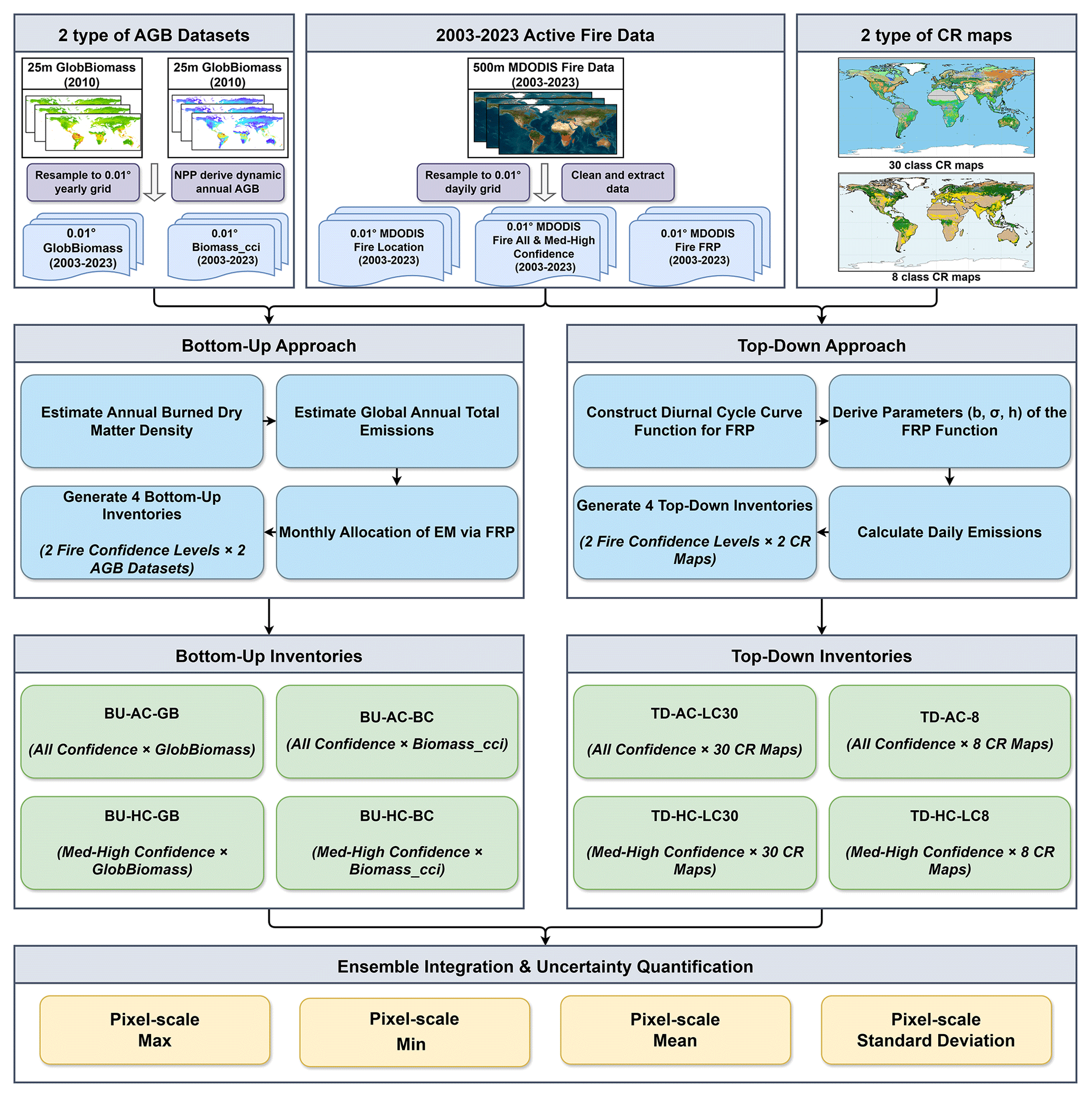
Figure 1 Framework for the construction of MBEI.

Table 2 The details of the eight biomass burning emission sub-inventories.

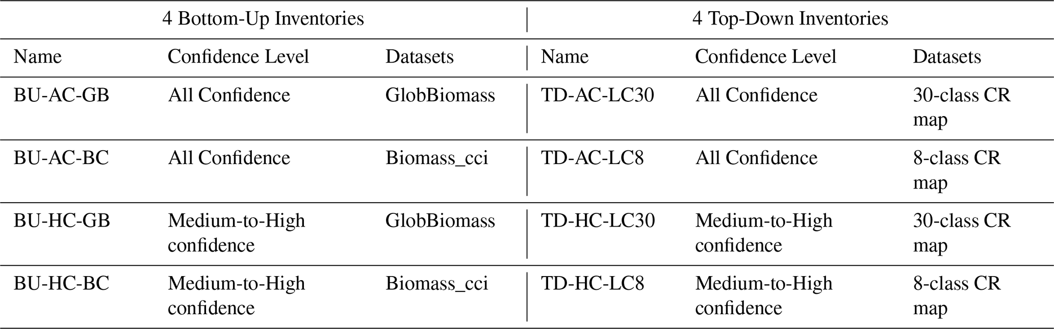
Note: The final MBEI dataset also includes the pixel-level ensemble statistics (Mean, Std, Max, Min) calculated from these eight sub-inventories.

2.2.1 Bottom-up emission estimation

This study employs a bottom-up method, combining multi-source remote sensing data to construct four global monthly biomass burning emission inventories for 2003–2023. The core computational workflow involves four key steps: (1) constructing a dynamic annual AGB dataset based on interannual variations in NPP; (2) modeling the total burned dry matter density (BD) under multiple fire events within a year; (3) estimating total annual emissions (EM) by burned area (BA), BD and EF; (4) downscaling annual emissions to a monthly resolution using the monthly distribution of FRP.

To overcome the limitation of using a static AGB benchmark map that ignores interannual variability, we constructed a dynamic annual AGB dataset. Based on the ecological assumption of a stable proportional relationship between AGB and NPP (Raich et al., 2006; Whittaker and Likens, 1973), we used the relative interannual changes in the MODIS annual NPP product to extrapolate the baseline AGB. The AGB for a target year (m) in a specific pixel (p) is calculated as:

$$\begin{array}{}\text{(1)}& {\mathrm{AGB}}_{\left(m,p\right)}={\mathrm{AGB}}_{\left(a,p\right)}\times {\displaystyle \frac{{\mathrm{NPP}}_{\left(m,p\right)}}{{\mathrm{NPP}}_{\left(a,p\right)}}}\end{array}$$

where AGB_(m,p) is the AGB in year m at pixel p (Mg ha⁻¹); AGB_(a,p) is the baseline AGB at pixel p (mean of 2003–2023, Mg ha⁻¹); NPP_(m,p) is the NPP in year m at pixel p (kg C m⁻² yr⁻¹); and NPP_(a,p) is the baseline mean NPP at pixel p (kg C m⁻² yr⁻¹).

After obtaining annual AGB, we estimated the annual BD per unit area. Considering that a pixel may experience multiple fires in a year, we used the following model to simulate the sequential consumption of AGB by fire and accumulate the total annual burned amount:

$$\begin{array}{}\text{(2)}& {\mathrm{BD}}_{\left(m,p\right)}=\sum _{j=\mathrm{1}}^{\mathrm{I}}{\mathrm{AGB}}_{\left(m,p\right)}\times {\left(\mathrm{1}-{\mathrm{BE}}_c\right)}^{j-\mathrm{1}}\times {\mathrm{BE}}_c\end{array}$$

where BD_(m,p) is the total burned dry matter density in year m at pixel p (kg m⁻²); I is the fire frequency in year m at pixel p (derived from active fire data); j represents the jth fire event of the year; AGB_(m,p) is the initial AGB at the beginning of the year (kg m⁻²); and BE_c is the dimensionless burning efficiency for the land cover type c of pixel p (derived from the Land Cover Type MCD12Q1.061).

The total annual emissions of each pollutant are estimated based on the method proposed by Seiler and Crutzen (1980):

$$\begin{array}{}\text{(3)}& {\mathrm{EM}}_{\left(m,p\right)}={\mathrm{BA}}_{\left(m,p\right)}\times {\mathrm{BD}}_{\left(m,p\right)}\times \mathrm{EF}\end{array}$$

where EM_(m,p) is the annual emission of a specific pollutant in year m at pixel p (g); BA_(m,p) is the total annual burned area in year m at pixel p (m²), obtained by multiplying the annual MODIS active fire location mask by the pixel's geographic area to ensure that the burned location is consistent with fire detections; BD_(m,p) is the annual burned dry matter density (kg m⁻²) calculated from Eq. (2); and EF is the emission factor for the specific pollutant (g kg⁻¹). It is important to note that inputs with annual temporal resolution (e.g., AGB, Land Cover-derived BE and EF) determine the magnitude of EM_(m,p) in this step and are not interpolated.

Finally, to obtain a monthly-resolution emission inventory, we applied a temporal allocation approach. We used satellite-observed FRP as a high-frequency proxy for fire activity intensity to distribute the total annual emissions EM_(m,p) into each month (t):

$$\begin{array}{}\text{(4)}& {\mathrm{EM}}_{\left(m,p,t\right)}={\mathrm{EM}}_{\left(m,p\right)}\times {\displaystyle \frac{{\mathrm{FRP}}_{\left(m,p,t\right)}}{{\sum }_{t=\mathrm{1}}^{\mathrm{12}}{\mathrm{FRP}}_{\left(m,p,t\right)}}}\end{array}$$

where EM${}_{(m,p,t)}$ is the pollutant emission in month t of year m at pixel p (g); and FRP${}_{(m,p,t)}$ is the monthly cumulative FRP in month t of year m at pixel p (MJ s⁻¹). This method ensures that while the total emission magnitude is constrained by annual fuel loads, the seasonality is driven by real-time fire radiative observations.

2.2.2 Top-down emission estimation

Our top-down emission estimation is based on the FRP approach, which uses satellite-observed thermal radiation to quantify biomass burning. The entire computational framework revolves around FRE, with the final pollutant emissions calculated as:

$$\begin{array}{}\text{(5)}& {\mathrm{EM}}_{\left(p\right)}={\mathrm{FRE}}_{\left(p\right)}\times {\mathrm{CR}}_{\left(r\right)}\times \mathrm{EF}\end{array}$$

where EM_(p) is the daily emission at pixel p (g); FRE_(p) is the daily cumulative FRE at pixel p (MJ); CR_(r) is the conversion factor for the biome r where pixel p is located (kg Dry Matter MJ⁻¹); and EF is the emission factor for the specific pollutant (g kg⁻¹).

However, polar-orbiting satellites like MODIS provide only limited observations per day, making it impossible to obtain daily cumulative FRE by simple integration of instantaneous FRP. To overcome this, we reconstruct the FRP diurnal cycle by fitting a Gaussian function, following the methodology of Vermote et al. (2009). We assume that the diurnal variation of FRP for a single biomass burning event can be represented by a Gaussian function:

$$\begin{array}{}\text{(6)}& \begin{array}{rl}{\mathrm{FRE}}_{\left(p\right)}& ={\int }_{\mathrm{0}}^{\mathrm{24}}\mathrm{FRP}{\left(t\right)}_{\left(p\right)}\mathrm{d}t\\ & ={\int }_{\mathrm{0}}^{\mathrm{24}}{\mathrm{FRP}}_{\mathrm{peak}\left(p\right)}\left(b+e^{-\frac{{\left(t-h\right)}^{\mathrm{2}}}{\mathrm{2}{\mathit{\sigma }}^{\mathrm{2}}}}\right)\mathrm{d}t\end{array}\end{array}$$

where FRP(t)_(p) is the instantaneous FRP at local time t for pixel p; FRP_peak(p) is the peak FRP of the fire event at pixel p (MJ s⁻¹); h is the local time of peak FRP hours; σ is the standard deviation of the Gaussian function, characterizing energy release concentration of the fire; and b is a background term reflecting residual or background radiation during non-active burning periods. The Gaussian parameters b, σ, and h are empirically derived for each biome from the long-term mean FRP ratio between Terra and Aqua observations using the relationships (henceforth $\frac{{\stackrel{\mathrm{‾}}{\mathrm{FRP}}}_{\mathrm{Terra}}}{{\stackrel{\mathrm{‾}}{\mathrm{FRP}}}_{\mathrm{Aqua}}}$):

$$\begin{array}{}\text{(7)}& {\displaystyle }b=\mathrm{0.86}\times {\left({\displaystyle \frac{{\stackrel{\mathrm{‾}}{\mathrm{FRP}}}_{\mathrm{Terra}}}{{\stackrel{\mathrm{‾}}{\mathrm{FRP}}}_{\mathrm{Aqua}}}}\right)}^{\mathrm{2}}-\mathrm{0.52}\times {\displaystyle \frac{{\stackrel{\mathrm{‾}}{\mathrm{FRP}}}_{\mathrm{Terra}}}{{\stackrel{\mathrm{‾}}{\mathrm{FRP}}}_{\mathrm{Aqua}}}}+\mathrm{0.08}\text{(8)}& {\displaystyle }\mathit{\sigma }=\mathrm{3.89}\times {\displaystyle \frac{{\stackrel{\mathrm{‾}}{\mathrm{FRP}}}_{\mathrm{Terra}}}{{\stackrel{\mathrm{‾}}{\mathrm{FRP}}}_{\mathrm{Aqua}}}}+\mathrm{1.03}\text{(9)}& {\displaystyle }h=-\mathrm{1.23}\times {\displaystyle \frac{{\stackrel{\mathrm{‾}}{\mathrm{FRP}}}_{\mathrm{Terra}}}{{\stackrel{\mathrm{‾}}{\mathrm{FRP}}}_{\mathrm{Aqua}}}}+\mathrm{14.57}\end{array}$$

where ${\stackrel{\mathrm{‾}}{\mathrm{FRP}}}_{\mathrm{Terra}}$ and ${\stackrel{\mathrm{‾}}{\mathrm{FRP}}}_{\mathrm{Aqua}}$ are the long-term mean FRP values for the respective sensors within that biome (MJ s⁻¹).

The final FRP_peak is determined by selecting either the daily peak FRP from the Aqua satellite (henceforth FRP_Aqua peak) or the daily peak FRP from the Terra satellite after correction with Eq. (12) (henceforth FRP_{Terra_corr}):

$$\begin{array}{}\text{(10)}& {\displaystyle }{\mathrm{FRP}}_{\mathrm{Aqua}{\mathrm{peak}}_{\left(p\right)}}={\displaystyle \frac{{\mathrm{FRP}}_{\mathrm{Aqua}\left(p\right)}}{\left(b+e^{-\frac{{\left(\mathrm{1.5}-\mathrm{h}\right)}^{\mathrm{2}}}{\mathrm{2}{\mathit{\sigma }}^{\mathrm{2}}}}\right)+\left(b+e^{-\frac{{\left(\mathrm{13.5}-\mathrm{h}\right)}^{\mathrm{2}}}{\mathrm{2}{\mathit{\sigma }}^{\mathrm{2}}}}\right)}}\text{(11)}& {\displaystyle }{\mathrm{FRP}}_{\mathrm{Terra}{\mathrm{peak}}_{\left(p\right)}}={\displaystyle \frac{{\mathrm{FRP}}_{\mathrm{Terra}\mathrm{\_}\mathrm{corr}\left(p\right)}}{\left(b+e^{-\frac{{\left(\mathrm{1.5}-\mathrm{h}\right)}^{\mathrm{2}}}{\mathrm{2}{\mathit{\sigma }}^{\mathrm{2}}}}\right)+\left(b+e^{-\frac{{\left(\mathrm{13.5}-\mathrm{h}\right)}^{\mathrm{2}}}{\mathrm{2}{\mathit{\sigma }}^{\mathrm{2}}}}\right)}}\text{(12)}& {\displaystyle }{\mathrm{FRP}}_{\mathrm{Terra}\mathrm{\_}\mathrm{corr}\left(p\right)}=\mathrm{FRP}{}_{\mathrm{Terra}\left(p\right)}\times {\displaystyle \frac{{\stackrel{\mathrm{‾}}{\mathrm{FRP}}}_{\mathrm{Terra}}}{{\stackrel{\mathrm{‾}}{\mathrm{FRP}}}_{\mathrm{Aqua}}}}\end{array}$$

where FRP_{Terra_corr(p)} is the corrected Terra FRP at pixel p (MJ s⁻¹), FRP_peak was calculated from Aqua satellite data using Eq. (10), following the approach of Vermote et al. (2009). Additionally, FRP values from the Terra satellite were adjusted using Eq. (12). This adjustment utilized long-term FRP ratios for different biomes to normalize the morning Terra observations to the afternoon measurement time of the Aqua satellite.

Independent daily FRE estimates were then calculated using the original Aqua observations (FRP_{Aqua peak(p)}) and the corrected Terra observations (FRE_{Terra peak(p)}) in Eq. (6) at pixel p (MJ s⁻¹). The final daily FRE is the average of these two estimates:

$$\begin{array}{}\text{(13)}& {\mathrm{FRE}}_{\left(p\right)}={\displaystyle \frac{{\mathrm{FRE}}_{\mathrm{Aqua}\left(p\right)}+{\mathrm{FRE}}_{\mathrm{Terra}\left(p\right)}}{\mathrm{2}}}\end{array}$$

Through these steps, we obtained the final daily FRE data. We then used Eq. (5) to calculate emissions and aggregated them to a monthly scale, ultimately producing four independent top-down emission inventories.

2.3 Trend analysis

Long-term trends in biomass burning emissions (2003–2022) were quantified using the Theil-Sen median trend estimator, with statistical significance assessed by the Mann–Kendall (MK) test (Mann, 1945; Sen, 1968). This non-parametric approach is particularly suitable for geophysical time series like emission data, as it is robust to outliers and does not assume a normal distribution.

The Theil-Sen estimator calculates the median of the slopes between all pairs of data points in the time series, making it robust to outliers (e.g., emission peaks from extreme fire years) and providing a stable estimate of the long-term trend. The slope is calculated as:

$$\begin{array}{}\text{(14)}& \mathrm{slope}=\mathrm{median}{\displaystyle \frac{x_j-x_i}{j-i}}\left(\mathrm{1}\le i<j\le n\right)\end{array}$$

where slope is the estimated trend, x_i and x_j are the data values at time points i and j, and n is the length of the time series.

3 Results

3.1 Spatial patterns and uncertainty of global biomass burning emissions

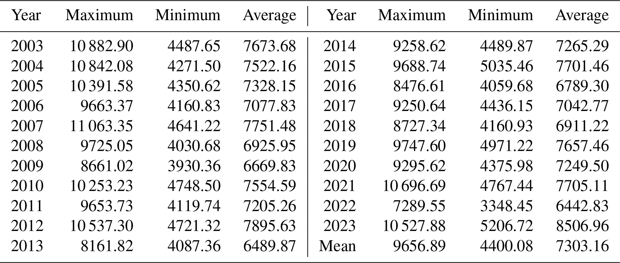
CO₂ is a principal greenhouse gas and the most widely studied species in biomass-burning inventories; accordingly, Sect. 3.1–3.4 focus on CO₂, and results for other species are provided in the Supplementary Information. For 2003 to 2023, the framework-mean global annual emissions for all species are summarized in Tables 3 and S5 The framework-mean CO₂ emission is 7303.63 Tg yr⁻¹, and the associated uncertainty, quantified as the range of annual means across the eight sub-inventories in the ensemble, spans 4400.08 to 9656.89 Tg yr⁻¹.

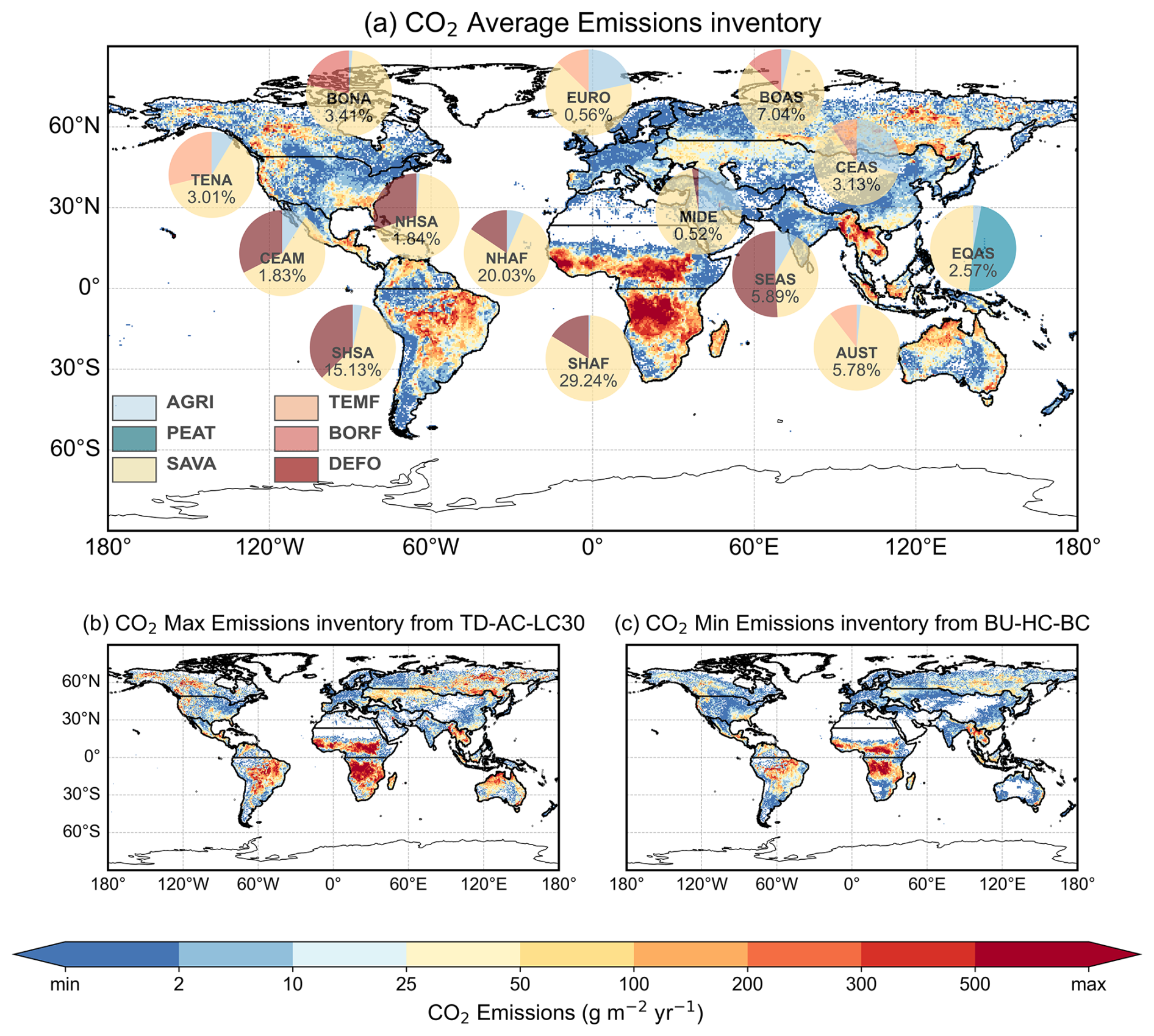
Figure 2 Spatial patterns and regional composition of global biomass burning CO₂ emissions (mean of 2003–2023). (a) Spatial distribution of the annual mean CO₂ emission flux estimated from the mean of the eight inventories in this study. The embedded pie charts show the emission composition for 14 major regions, where: (1) the number in the pie chart indicates the percentage of that region's emissions relative to the global total; and (2) the sectors of the pie chart represent the proportional contribution of six major fire types to the region's total emissions. (b) and (c) show the spatial emission patterns corresponding to the inventory with the highest global total annual emissions (TD-AC-LC30) and the lowest global total annual emissions (BU-HC-BC) among the eight inventories over the entire study period, respectively.

Figure 2 shows the highly heterogeneous spatial pattern of mean annual CO₂ emission fluxes (the spatial patterns for other major pollutants are presented in Fig. S6). Global emission activities are largely concentrated in tropical and subtropical regions, characterized by high emission fluxes (> 300 g m⁻² yr⁻¹). Within these areas, the most intense emission hotspots (> 500 g m⁻² yr⁻¹) are clearly identified over the Congo Basin, surrounding savannas, and parts of Southern Africa. This high spatial concentration of intense burning directly translates to Africa's dominant role in the global emission budget. Based on regional statistics (Global 14 regions defined in Fig. S3), Southern Hemisphere South Africa (SHAF) and Northern Hemisphere South Africa (NHAF) collectively contribute 49.2 % of global CO₂ emissions (29.2 % and 20.0 %, respectively). Furthermore, Southern Hemisphere South America (SHSA, 15.1 %), Boreal Asia (BOAS, 7.0 %), and Southeast Asia (SEAS, 5.9 %) also stand out as major source regions for global biomass burning.

The dominant types of biomass burning vary substantially by region (see Fig. S4 for the classification of fire types), leading to distinct emission profiles (see Fig. S5 for the composition of fire types in each region). In the top three emitting regions (SHAF, NHAF, and SHSA), which collectively account for nearly two-thirds (64.4 %) of global CO₂ emissions, burning is driven primarily by savanna fires (SAVA) and deforestation fires (DEFO). The contribution of different fire types varies significantly among these top regions (see Fig. 2a for detailed emission values). In SHAF, the largest source, SAVA are overwhelmingly dominant, accounting for 83 % of its CO₂ emissions. A similar pattern occurs in NHAF, where SAVA contributes 78 % of emissions, although agricultural waste burning (AGRI) also plays a notable role (6 %). In contrast, the emissions in SHSA are more evenly split between SAVA (59 %) and DEFO fires (37 %). In the high-latitude regions of BOAS and Boreal North America (BONA), fires in boreal forests (BORF) are a characteristic emission source, contributing 14 % and 22 % of regional CO₂ emissions, respectively. Notably, our analysis identifies fires classified as SAVA as the largest contributor in both regions (83 % in BOAS and 77 % in BONA). It is critical to note that SAVA in this context refers to the burning of extensive grasslands and shrublands located within the boreal climate zone, as defined by our underlying land cover dataset, rather than tropical savannas. This highlights that non-forest fires are the dominant source of emissions even in these high-latitude zones.

The emission composition of Equatorial Asia (EQAS) is unique. Although its total emissions are relatively low, it is the only region dominated by peatland fires (PEAT), with PEAT emissions contributing as much as 91.34 Tg yr⁻¹ of CO₂ (48.4 % of the regional total). This uniqueness stems from its specific fire regime: vast areas of organic-rich peatlands become highly flammable after being drained and converted to agricultural land (e.g., oil palm plantations). Such fires often manifest as long-duration, hard-to-extinguish subsurface smoldering, leading to extremely high carbon emission intensities and making EQAS a unique and closely watched case in global biomass burning research.

The spatial heterogeneity of this uncertainty is illustrated in Fig. 2b and c, which map the highest and lowest emission estimates across the ensemble. Globally, the uncertainty is substantial, with the maximum estimate of annual CO₂ emissions being 2.2 times higher than the minimum estimate across the MBEI sub-inventories.

Importantly, high biomass burning emission uncertainty is not found in traditional biomass burning hotspots. Instead, some of the highest uncertainties are found in regions with lower overall emissions. Specifically, Australia and New Zealand (AUST) and the Middle East (MIDE) exhibit the greatest uncertainty, with maximum-to-minimum (max/min) emission ratios reaching 7.18 and 6.40, respectively. In AUST, this extreme uncertainty is linked to its fire regime dominated by highly intermittent and catastrophic megafires (e.g., the 2019–2020 events), which pose significant challenges to consistent estimation across different algorithms. In MIDE, which contributes only 0.52 % to the global total, the high uncertainty stems from small, scattered AGRI and SAVA. These weak fire signals are near the lower limit of satellite detection capabilities, a fact confirmed by the large discrepancy observed when comparing estimates derived from “all confidence” versus “high and medium confidence” active fire data. In contrast, the major tropical burning regions show much lower relative uncertainty, despite their massive contribution to global emissions. The African (SHAF, NHAF) and South American (SHSA) hotspots have $\max /\min$ ratios consistently below 2.0. This greater consensus among methods is attributable to the nature of their fires: large-scale, intense, and seasonally predictable SAVA that are robustly captured by various estimation approaches. Meanwhile, temperate and high-latitude regions such as Central Asia (CEAS), BONA, and Europe (EURO) show intermediate levels of uncertainty, with $\max /\min$ ratios between 3.5 and 4.0.

In summary, this analysis reveals a critical divergence between the spatial patterns of emission magnitudes and their estimation uncertainties. While emission hotspots are concentrated in tropical regions dominated by regular SAVA and DEFO, the highest uncertainties occur in areas characterized by either highly intermittent megafires (e.g., AUST) or weak, scattered burning (e.g., MIDE), posing distinct challenges to current estimation methods.

Table 3 Total annual CO₂ emissions (Maximum, Minimum, and Average, unit: Tg) for 2003–2023.

3.2 Seasonality of biomass burning emissions

The MBEI 2003–2023 CO₂ emission inventory reveals a distinct bimodal seasonal cycle (Fig. 3a). Global emissions reach a minimum in February and then climb to a primary peak in the Northern Hemisphere's late summer (August–September). This global pattern results from the combined effect of staggered fire seasons in key regions. Four regions in particular (SHAF, NHAF, SHSA, and BOAS) drive this cycle, collectively accounting for over 71 % of total annual emissions (Fig. 3b). For a detailed view of the emission sources, Fig. S7 shows the monthly composition of CO₂ emissions by the six fire types for each of the 14 global regions during 2003–2023.

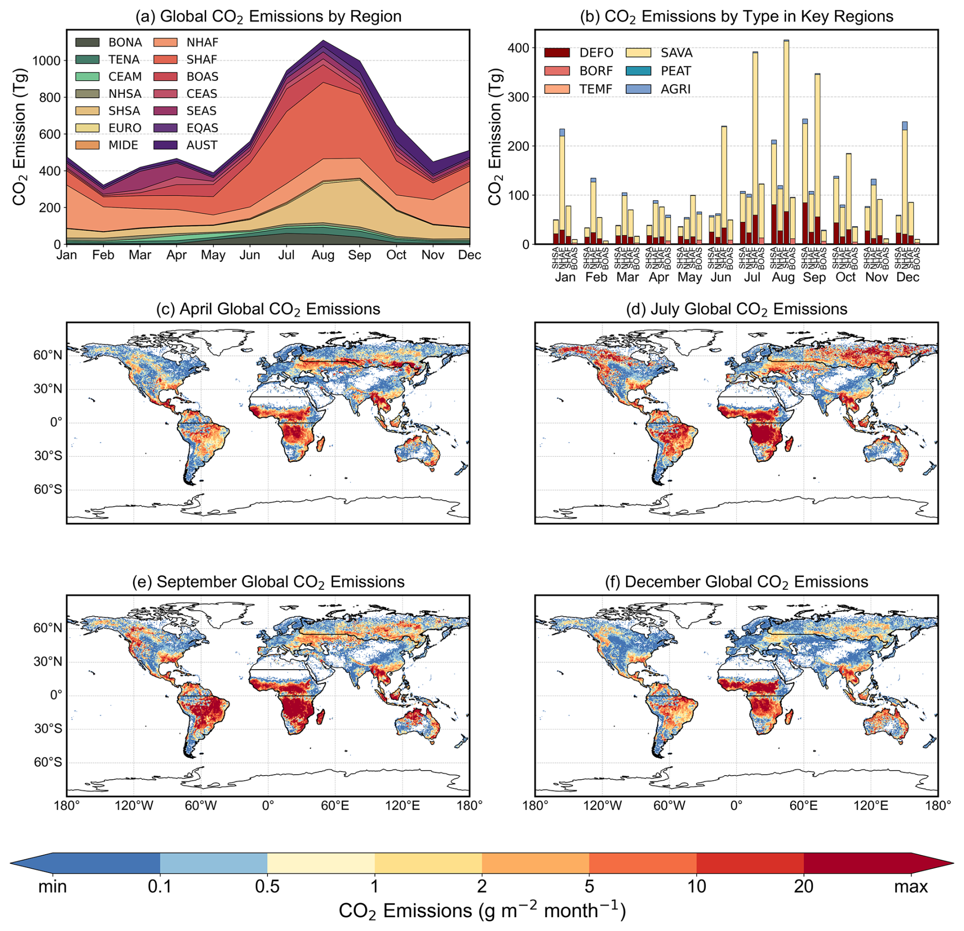
Figure 3 Seasonal cycle and spatial dynamics of global biomass burning CO₂ emissions (mean of 2003–2023). (a) Global monthly emissions partitioned by source region. (b) Monthly emissions for the four primary contributing regions, showing the composition by fire type. (c–f) Spatial distribution of mean monthly emission flux during key seasonal phases: April, July, September, and December.

The annual cycle begins its ascent after the global minimum in February, initially driven by fire activity in the Northern Hemisphere. Persistent dry-season burning in NHAF transitions into an intensifying fire season across Eurasia. By April, the focus of burning activity clearly shifts northward, with emissions surging in regions like BOAS, while the major Southern Hemisphere burning regions (SHAF and SHSA) remain in a period of low activity (Fig. 3c).

From May onwards, global emissions accelerate rapidly, driven by the increasing overlap of fire seasons in both hemispheres. While boreal fires in regions like BOAS reach their annual peak in July, the dominant driver of this global surge is the explosive onset of the fire season in SHAF. Concurrently, burning intensifies in SHSA, and this synergistic effect pushes global emissions towards their annual maximum (Fig. 3d).

The global emission peak in August and September is dominated by the Southern Hemisphere, as fire activity wanes in the major Northern Hemisphere regions. During this period, burning in SHSA reaches its annual zenith, fueled by a combination of DEFO and SAVA. Although past its own peak, SHAF remains the single largest regional contributor to global emissions (Fig. 3e).

Beginning in October, the onset of the rainy season in the Southern Hemisphere rapidly suppresses fire activity there, causing a sharp decline in global emissions. This marks a decisive shift in the global burning pattern. The focus of activity returns entirely to NHAF, which enters its primary fire season that lasts through the subsequent winter (Fig. 3f). This distinct hemispheric seesaw effect completes the annual cycle. Figure S8 presents the spatial distribution patterns of monthly CO₂ emissions from global biomass burning during the period 2003–2023.

3.3 Interannual variability and long-term trends

Over the 2003–2023 study period, global biomass burning CO₂ emissions are characterized not by a significant long-term trend but by pronounced interannual variability. Specifically, the time series of global annual CO₂ emissions, derived from the MBEI, which integrates eight sub-inventories, shows no statistically significant long-term trend (p > 0.05; Fig. 4a). This pattern of high interannual variability, coupled with a lack of a significant long-term trend, is also observed for other major emitted species (Fig. S9). This strong interannual variability is a well-documented feature of global fire activity, primarily linked to climate anomalies such as the El Niño-Southern Oscillation (ENSO) (Chen et al., 2017; Mariani et al., 2016; Li et al., 2023). Our time-series analysis confirms this link: emission peaks (e.g., 2010, 2015, 2019) consistently coincide with major El Niño events that trigger widespread drought, while emission troughs (e.g., 2009, 2022) align with wetter La Niña conditions. The sharp contrast between the low emissions during the 2022 La Niña and the subsequent spike during the 2023 El Niño starkly illustrates the powerful influence of the ENSO cycle on global fire activity.

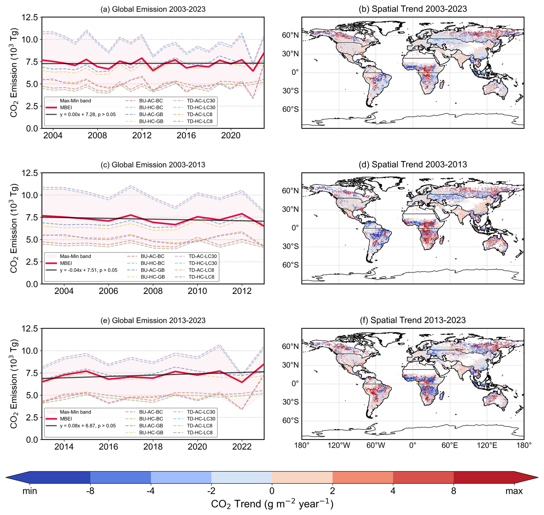
Figure 4 Temporal and spatial trends of global biomass burning CO₂ emissions from 2003 to 2023. (a, c, e) Interannual variation of total emissions and (b, d, f) trends in emission flux for three periods: 2003–2023, 2003–2013, and 2013–2023.

Alongside these climate-driven variations, the MBEI is characterized by a broad uncertainty range, stemming from differences in algorithm structures and input data. The spread between MBEI estimates (the Max–Min band in Fig. 4a, c, e) is considerable, with the difference between the highest and lowest annual totals exceeding 2600 Tg in some years (e.g., 2004, 2022). This divergence arises from methodological differences, particularly between top-down (FRP-based) and bottom-up (burned area-based) approaches in areas like fire detection and combustion parameterization. Critically, however, despite the large spread in absolute emission values, the MBEI sub-inventories show strong agreement on the relative interannual patterns, consistently identifying the same peak and trough years.

This apparent global stability masks significant and opposing regional trends, producing a highly heterogeneous spatial pattern of change (Fig. 4b). Over the full 21-year period, statistically significant trends were concentrated in Asia. BOAS exhibited a strong and significant increasing trend in emission flux at a rate of 15.71 g m⁻² yr⁻¹ (p<0.01). In contrast, CEAS and SEAS showed significant decreasing trends of −1.72 g m⁻² yr⁻¹ (p<0.01) and −2.08 g m⁻² yr⁻¹ (p<0.05), respectively (Table S6). Figure 4b suggests decreases in equatorial Africa and central-southern South America, and increases in BONA, these trends were not statistically significant when aggregated over the entire 14 GFED regions for the 2003–2023 period. This highlights an offsetting pattern, where declining emissions in some regions are partially balanced by increases elsewhere, contributing to the lack of a significant global trend.

A decadal comparison between 2003–2013 and 2013–2023 reveals substantial evolution in these spatial patterns, indicating a major shift in the global distribution of biomass burning emissions (Fig. 4d, f).

During the first decade (2003–2013), a slight but statistically non-significant global decrease (p > 0.05; Fig. 4c) masked a profound spatial redistribution of fire activity. The dominant feature was a significant increase in fire emissions in SHAF, which saw an upward trend of 4.41 g m⁻² yr⁻¹ (p< 0.05). By contrast, South America experienced significant decreases, particularly in NHSA where emissions declined at a rate of −4.97 g m⁻² yr⁻¹ (p< 0.05). Simultaneously, a strong decreasing trend was observed in CEAS, with a rate of −2.96 g m⁻² yr⁻¹ (p< 0.05). Boreal regions and Southeast Asia showed no statistically significant regional trends during this period (Fig. 4d and Table S7).

In the subsequent decade (2013–2023), this pattern shifted markedly. Although the global emission trajectory did not exhibit a statistically significant linear trend (p > 0.05), it transitioned from a slight decline to an overall increase (Fig. 4e), signaling a clear decadal change in biomass burning dynamics. This shift is more appropriately characterized as a structural transformation rather than a linear progression, driven by a marked increase in both the frequency and intensity of extreme emission years (e.g., 2015, 2019, 2023). The 2015–2016 ENSO cycle exemplifies this mechanism, as the super El Niño event in 2015 induced catastrophic PEAT in Indonesia (EQAS) and elevated global emissions to a record peak, which was subsequently followed by a pronounced decline in 2016 with the onset of a strong La Niña (Whitburn et al., 2016; Yin et al., 2020a). The 2023 fire season was even more pronounced, as an unprecedented wildfire season in boreal Canada (BONA) coincided with a developing El Niño, jointly driving global annual emissions to the highest level in our 21-year record. Detailed regional statistics, including the annual mean CO₂ emission fluxes and their corresponding Theil-Sen slope trends across the 14 study regions for the 2013–2023 period, are summarized in Table S8 (Jain et al., 2024; Luo et al., 2025).

Spatially, this decadal shift is characterized by a reversal of trends in Africa and South America (Fig. 4f). Africa, which previously showed increasing trends in the south, now exhibited a pronounced and significant decrease in NHAF, with emissions declining at −5.14 g m⁻² yr⁻¹ (p< 0.05). In a direct reversal of the previous decade, SHSA showed a strong and significant increase of 8.01 g m⁻² yr⁻¹ (p<0.01). Notably, despite the visually striking increases in BONA and northern Eurasia driven by the extreme fire years mentioned previously, the linear trends for these aggregated regions over the 2013–2023 period were not statistically significant, suggesting that the changes were dominated by episodic events rather than a consistent year-over-year increase.

In summary, beneath the overall stable trend of global biomass burning emissions over the past 21 years, there lies a key decadal shift, from a declining phase dominated by weakening fire activity in the tropics (2003–2013) to an increasing phase driven by intensifying fire activity in high-latitude regions and parts of the Southern Hemisphere (2013–2023).

3.4 Inter-comparison with other inventories

A comparison of biomass burning CO₂ emissions reveals broad spatial agreement across all inventories (including the MBEI from this study, FINN 2.5, GFAS 1.2, GFED 5.0, and QFED 3.1) (Fig. 5). Furthermore, the emission magnitudes from these inventories are largely consistent, with no significant discrepancies. In addition, comparative analyses are performed for three emission species, namely SO₂, PM_2.5 and BC and the results are presented in Figs. S10–S15. These species represent different components and combustion phases of biomass burning. SO₂ reflects the combustion of naturally occurring sulfur-containing organic matter and inorganic sulfides in biomass, PM_2.5 represents the overall intensity of total particulate matter emissions, and BC indicates incomplete combustion during the high-temperature flaming phase. Similar to CO₂, the spatial patterns for these species are largely consistent across inventories. While the products capture similar interannual variability, their estimates of emission magnitudes reveal substantial inter-inventory uncertainty (results show in Figs. S10–S15). All products successfully identify the primary global fire hotspots, including those in Africa (SHAF, NHAF), South America (SHSA), Southeast Asia (SEAS), and the northern boreal forests (BONA, BOAS).

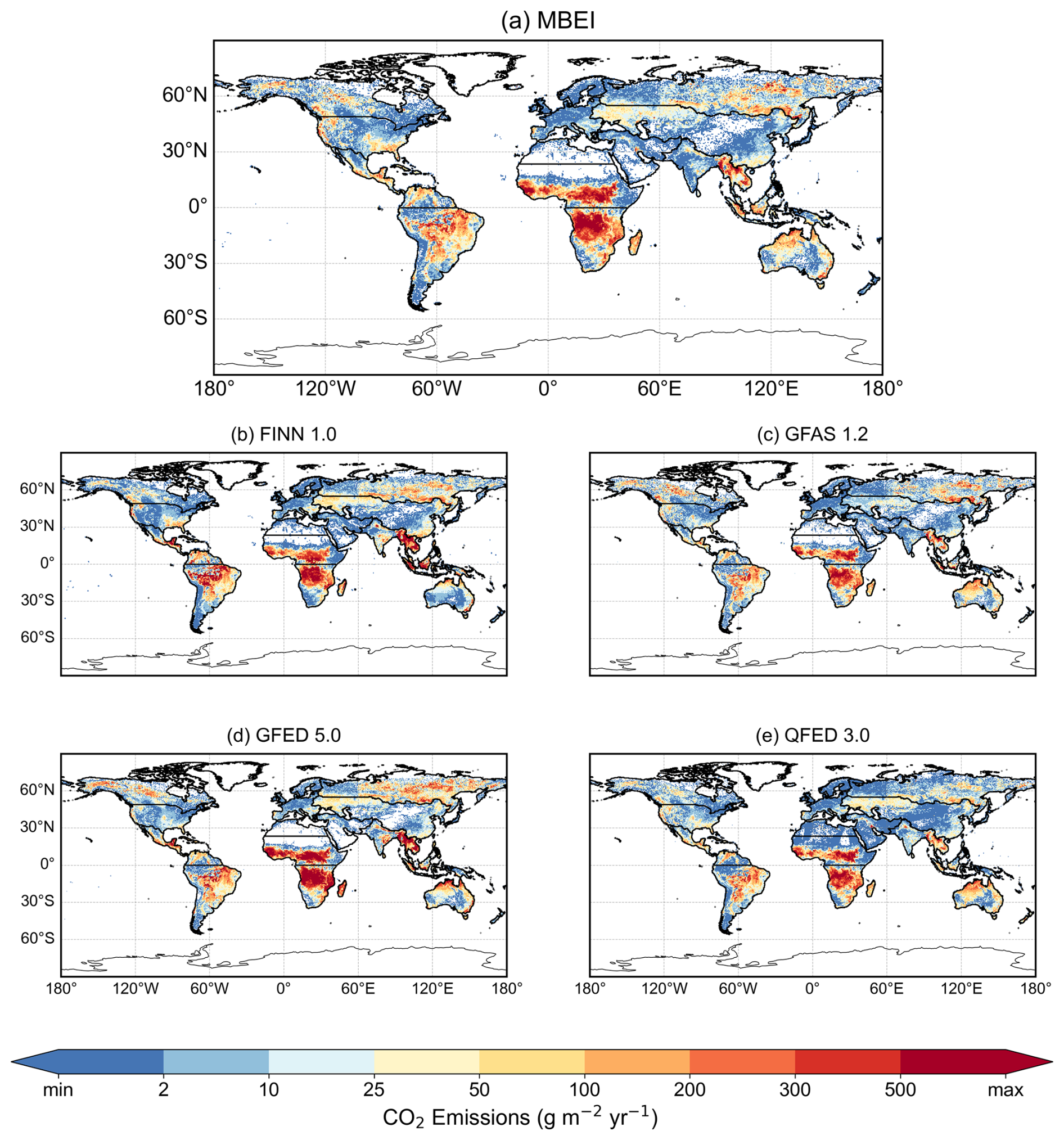
Figure 5 Comparison of multi-year mean spatial patterns of global CO₂ emissions estimated by different biomass burning inventories (2003–2022). (a) The mean of the eight inventories constructed in this study. (b) Fire INventory from NCAR version 2.5 (FINN 2.5), (c) Global Fire Assimilation System version 1.2 (GFAS 1.2), (d) Global Fire Emissions Database version 5.0 (GFED 5.0), and (e) Quick Fire Emissions Dataset version 3.1 (QFED 3.1).

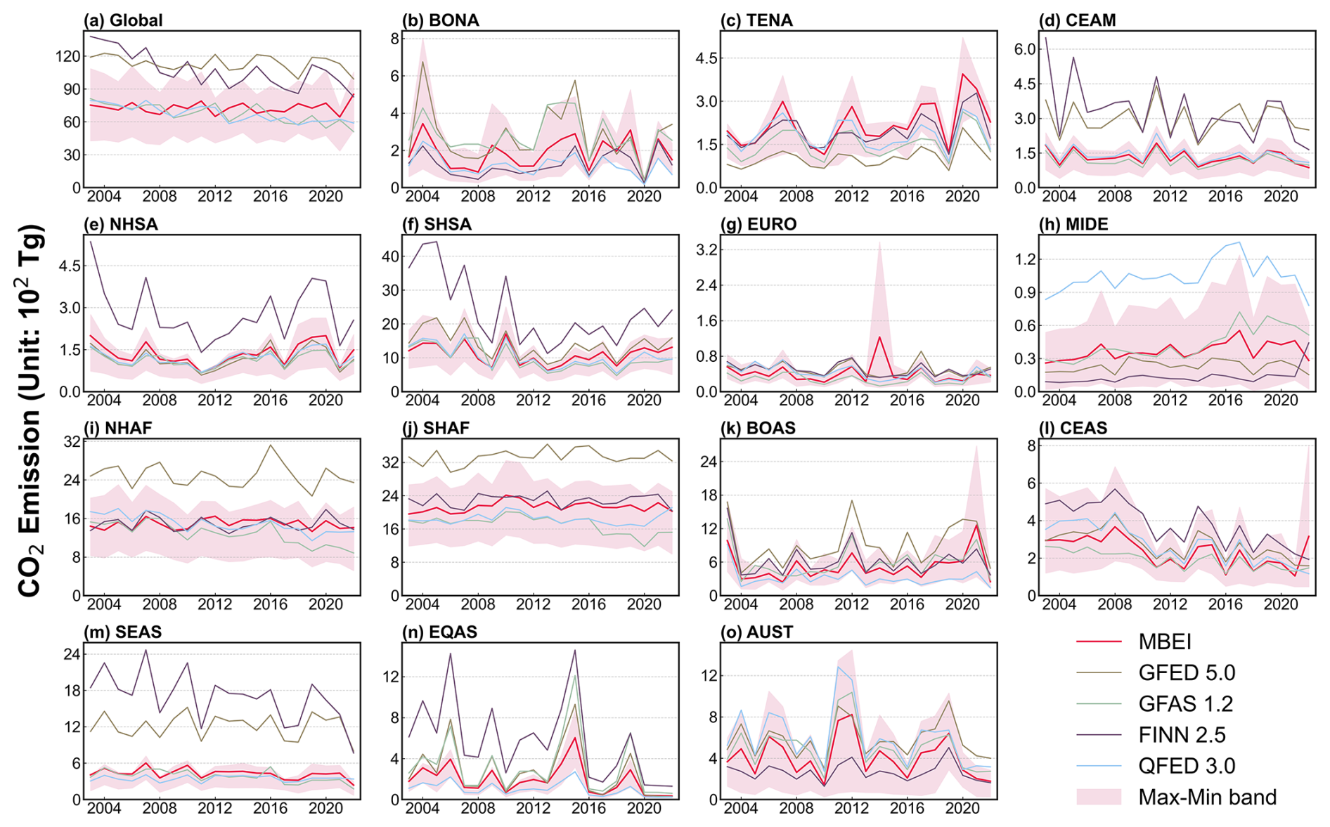
Figure 6 Time series of interannual variability in biomass burning CO₂ emissions from different inventories at global and regional scales (2003–2022). (a) Total annual global CO₂ emissions from this study's inventory and four other inventories. (b) to (o) Total annual CO₂ emissions from this study's inventory and four other inventories across 14 regions.

However, significant discrepancies exist in both emission magnitude and spatial detail among various inventories (Fig. 6). The uncertainty range (Max–Min band) of the MBEI generally encompasses the estimates from all reference products across most regions, suggesting that it effectively captures the structural uncertainty among inventories. Moreover, the mean estimate of the MBEI typically resides near the center of the various inventories. With respect to magnitude and trend, our inventory exhibits the closest alignment with GFAS. GFED consistently provides the highest global estimates, while FINN ranks second and in some regions even exceeds GFED, whereas QFED remains generally lower. Despite these differences in magnitude, all inventories demonstrate strong consistency in interannual variability, successfully capturing major global fire years (e.g., 2010, 2015, 2019).

A regional analysis highlights significant divergences among emission inventories, particularly in the high-emission tropics where the MBEI's uncertainty band is often substantial. In the African savannas (NHAF, SHAF), the MBEI mean estimate is consistently lower than GFED 5.0, often residing in the lower half of the inter-inventory range (Fig. 6i, j). For instance, in SHAF, GFED 5.0 estimates are frequently approximately 10 Tg yr⁻¹ higher than the MBEI mean, while our estimate aligns closely with GFAS 1.2 and QFED 3.0. Conversely, in regions with significant DEFO and AGRI fires like SHSA and SEAS, FINN 2.5 estimates consistently occupy the upper portion of the inter-inventory range. In these areas, the MBEI mean is again more conservative, and our Max–Min band effectively captures the cluster of lower estimates from GFED, GFAS, and QFED (Fig. 6f, m).

In contrast, inter-inventory agreement is generally higher in low- to moderate-emission regions at mid- to high latitudes, where the MBEI mean closely tracks the multi-inventory average (e.g., Temperate North American (TENA) and EURO; Fig. 6c, g). However, this consistency breaks down in boreal forests during years with episodic, large-scale fires. In these instances, the value of the Max–Min band becomes particularly evident. During the extreme BONA fire year of 2004, estimates spanned a wide range from FINN 2.5 (2.2 Tg) to GFED 5.0 (6.7 Tg). Critically, our own Max–Min band for that year expanded dramatically (from 1.0 to 8.0 Tg), explicitly quantifying the immense challenge and uncertainty in capturing such events. A similar expansion of our uncertainty band is observed in BOAS during its severe 2021 fire season, where our maximum estimate reached 26.8 Tg, encompassing the high values from other inventories.

Regions dominated by specific fuel types, such as the peatlands of EQAS, reveal fundamental methodological differences that are well-framed by our uncertainty analysis. While all inventories captured the 2015 El Niño-driven fire peak, the estimated magnitude varied by more than five-fold, from QFED 3.0 (2.7 Tg) to FINN 2.5 (14.6 Tg) (Fig. 6n). The MBEI mean estimate (6.0 Tg) and its associated uncertainty band (3.2–8.6 Tg) are positioned centrally among these estimates, with its upper bound approaching the GFED 5.0 value (9.3 Tg) while excluding the extreme high and low outliers. This indicates that, under substantial uncertainty in quantifying PEAT emissions, the MBEI delineates a comprehensive Max–Min band and provides a stable central mean estimate within it.

In summary, our comparison demonstrates that while existing inventories agree on broad spatiotemporal patterns, significant quantitative disagreements persist, particularly in tropical regions and during extreme fire events. Against this backdrop, the MBEI provides a new, synthesized central estimate and a robust uncertainty range (Max–Min band). Its central estimate is consistent with the ensemble median, and its uncertainty bounds effectively encompass the spread across different inventories. This central estimate and a quantified uncertainty range not only offers a reliable measure of biomass burning emissions but also serves as a diagnostic tool, highlighting the specific regions (e.g., African savannas, Southeast Asian peatlands) and conditions (e.g., extreme boreal fires) that drive the largest inter-inventory discrepancies, thereby providing a clear basis for future inventory refinement.

4 Discussion

4.1 Advancement and uncertainty assessment

This study introduces the MBEI, a systematic emission estimation framework built upon a framework of eight sub-inventories, integrating both bottom-up and top-down approaches with various combinations of key input data. The emission range of the MBEI provides a direct measure of structural uncertainty, allowing modelers to assess the sensitivity of their simulations to inventory choice (high-end vs. low-end estimates). This addresses a long-standing challenge in climate and atmospheric chemistry modeling, where discrepancies among emission inventories are a recognized major source of the simulation uncertainty (Pan et al., 2020; Su et al., 2023). The MBEI framework systematically quantifies this uncertainty, revealing two key findings. First, the uncertainty is substantial in magnitude, with the maximum global annual CO₂ estimate across the sub-inventories being 2.2 times the minimum. Second, and perhaps more importantly, the uncertainty exhibits significant spatial heterogeneity, with the highest relative uncertainty not coinciding with traditional emission hotspots, but instead found in regions with lower emissions, such as AUST and MIDE.

This divergence is strongly linked to how regional land cover and fire regime characteristics amplify the sensitivity of different estimation methodologies. For instance, in AUST, the fire regime is dominated by event-driven, extremely high-intensity megafires. These events pose significant challenges for both FRP-based algorithms, which can be prone to saturation, and burned area-based methods, which struggle to accurately map such intense and rapidly spreading fires. Conversely, in the MIDE, the high uncertainty arises from weak, small-scale, and scattered AGRI or SAVA. These fires are often near the detection limits of satellite sensors, causing emission estimates to be highly sensitive to the chosen active fire detection confidence thresholds. In stark contrast, African savannas, despite their high emission fluxes, show lower relative uncertainty. Their widespread and seasonally predictable fires are robustly captured by both top-down and bottom-up approaches, leading to greater convergence among the different methods. This finding implies that future efforts to refine emission inventories should extend beyond traditional hotspots to better understand and parameterize the distinct combustion processes in these atypical fire regimes.

The MBEI's 21-year analysis also uncovers a critical shift in the long-term dynamics of global emissions. Despite a stable trend overall, we identify a clear decadal transition: from a slight decline dominated by weakening tropical fires (2003–2013) to a rising phase driven by intensifying boreal fires and more frequent extreme events (2013–2023). This dynamic, characterized by a decline in tropical fire activity and an increase in boreal fire activity, synthesizes seemingly disparate observations, such as the global decrease in burned area (Andela et al., 2017) and the lengthening of fire seasons in high-latitude regions (Jones et al., 2022), into a coherent narrative at the emission level. Particularly in the second decade, climate-driven extreme events, such as the 2015 Indonesian peat fires, the 2019–2020 Australian megafires, and the 2023 Canadian wildfires, significantly reshaped the global emission record. This underscores the growing influence of climate change on global biomass burning emissions, a shift with profound implications for the global carbon cycle and its associated climate feedbacks.

4.2 Limitations and Future Perspectives of the MBEI Framework

The MBEI framework aims to quantify the structural uncertainty in global biomass burning emissions by ensembling multiple algorithmic approaches. However, the accuracy of any emission inventory is inherently constrained by the spatiotemporal resolution and physical sensitivity of its input data. The uncertainty ranges revealed in this study, which span various regions and biomes, largely reflect the physical limitations of current Earth observation systems in capturing extreme fire behaviors and complex surface processes, alongside the methodological differences discussed.

A key decision in this study was to use MODIS active fire products (MCD14DL) exclusively for the 2003–2023 period. Although the Visible Infrared Imaging Radiometer Suite (VIIRS), available since 2012, offers superior spatial resolution (375 m) compared to MODIS (1 km), applying it would have limited the consistent time series to the post-2012 era. Merging MODIS (2003–2011) and VIIRS (2012–2023) records introduces a risk of inconsistency; the higher detection sensitivity of VIIRS could result in an artificial increase in fire counts, which might be misinterpreted as a real upward trend in global fire activity. To maintain the homogeneity of the 21-year dataset for trend analysis, we prioritized sensor consistency. We acknowledge that this choice likely leads to an underestimation of emissions from small-scale agricultural fires, particularly in regions like the Middle East or India, where fires are often smaller than the MODIS detection threshold (Hantson et al., 2013; Justice et al., 2002; Vadrevu and Lasko, 2018).

In addition to sensor specifications, most current inventories relying on optical remote sensing face inherent physical limits driven by environmental heterogeneity. Complex surface conditions can constrain the effectiveness of estimation methods. For instance, in the peatlands of Equatorial Asia (e.g., Indonesia), fires often occur as subsurface low-temperature smoldering. The thermal radiation from these fires is frequently too weak to trigger standard satellite detection algorithms (Rein and Huang, 2021; Sofan et al., 2019). Similarly, in dense tropical rainforests, the canopy layer can occlude or absorb thermal radiation emitted by understory fires (East et al., 2023). These scenarios contribute to omission errors in top-down, FRP-based approaches (Morton et al., 2013; Tyukavina et al., 2022). Conversely, while bottom-up methods based on burned area can capture the spatial traces of these fires, they face challenges in accurately determining the depth of burn in organic soils (Ballhorn et al., 2009; Wiggins et al., 2018). Therefore, despite the integration of multiple algorithms in MBEI, these physical constraints suggest a potential underestimation in our emission estimates for these specific biomes.

Looking forward, the flexible architecture of MBEI is designed to incorporate emerging datasets to address these limitations. As the observational record of VIIRS extends, future versions of MBEI will integrate these data to improve the detection of small-scale fires once a sufficiently long and consistent record is established. Furthermore, data from new-generation geostationary satellites (e.g., FY-4, Himawari-8/9, GOES-R) offer a significant improvement in temporal resolution. Minute-level observations from these platforms will enable the direct integration of the Fire Radiative Power diurnal cycle, reducing the reliance on Gaussian extrapolation from sparse polar-orbiter snapshots and enhancing the physical realism of Fire Radiative Energy estimation.

Advancements in next-generation satellites will also enhance the MBEI's capacity for fuel load estimation. In this study, due to the lack of high-resolution annual AGB observations, we adjusted static AGB maps using interannual variations in NPP. However, AGB is a cumulative stock variable, whereas NPP is an annual flux variable. Their relationship is complex and influenced by factors such as lag effects, tree mortality, and decomposition, meaning a high NPP year does not always result in an immediate biomass increase (Keeling and Phillips, 2007; Teets et al., 2022). Future versions of MBEI aim to improve this by integrating dynamic AGB datasets from active remote sensing missions. Specifically, spaceborne LiDAR (e.g., NASA GEDI) and P-band SAR (e.g., ESA BIOMASS mission) are expected to provide global measurements of forest vertical structure. This will allow MBEI to incorporate dynamic fuel loads, thereby reducing a major source of uncertainty in the bottom-up approach based on burned area (Cao et al., 2016; Liu et al., 2019; Rodríguez-Fernández et al., 2018).

Finally, current emission estimates rely on static EFs, which may not fully capture the variability of combustion efficiency within biomes or during a fire's lifecycle (van Leeuwen et al., 2013; Yin, 2022). Future improvements are expected to come from developing comprehensive EF databases through advanced molecular-level aerosol speciation (Jen et al., 2019; Koss et al., 2018). Complementing this, dynamic high-resolution EF datasets could be generated using synchronous satellite trace gas retrievals. For example, the ratio of carbon monoxide to nitrogen dioxide (ΔNO${}_{\mathrm{2}}/\mathrm{\Delta }$CO) columns derived from the TROPOMI sensor can serve as a near-real-time proxy for combustion efficiency (flaming vs. smoldering) (van der Velde et al., 2021). By assimilating such dynamic proxies, MBEI aims to evolve toward a more dynamic monitoring system.

In conclusion, while the current version of MBEI quantifies uncertainty by integrating established methods, its modular design serves as a platform for incorporating new data inputs as they become available. This ensures a feasible pathway for iterative refinement, supporting more comprehensive assessments of global biomass burning emissions.

5 Data availability

The developed MBEI emission inventory described in this paper is available from https://doi.org/10.5281/zenodo.18104830 (Liu and Yin, 2025). For further support or guidance regarding data use, please contact yinshuai@aircas.ac.cn.

6 Conclusion

This study systematically assessed global biomass burning emissions and their uncertainties from 2003–2023 using the MBEI, an ensemble framework of eight sub-inventories that integrates both bottom-up and top-down approaches. A key finding is the spatial separation between the emission hotspots and the uncertainty hotspots. While high-emission regions in Africa and South America account for 64.4 % of global CO₂ emissions, the structural uncertainty there is relatively constrained ($\max /\min$ ratio < 2.0). In contrast, the greatest uncertainty ($\max /\min$ ratio > 6.0) is found in lower-emission regions characterized by extreme, intermittent fires (e.g., AUST) or scattered agricultural burning (e.g., the MIDE).

Temporally, our analysis reveals a significant shift in the drivers of global biomass burning emissions over the past two decades. Although the overall long-term trend is not statistically significant, we identify a clear transition: the period dominated by declining tropical fire activity (2003–2013) was followed by a period increasingly influenced by intensifying high-latitude boreal fires and frequent climate-driven extreme events (2013–2023).

The spatial heterogeneity and temporal shift highlight the growing complexity of the global biomass burning emission regimes. The primary contribution of the MBEI framework is therefore its ability to explicitly quantify this structural uncertainty. It provides a central estimate consistent with the multi-inventory average, along with an uncertainty range that encompasses the estimates of major existing products. MBEI offers the crucial boundary conditions needed for Earth system models to estimate related environmental or exposure risk.

To effectively assess the complex dynamics of global biomass burning emission, the results of this study indicate that the focus should evolve from pursuing a single best estimate to embracing a probabilistic, uncertainty-aware approach. It is suggested that such data-constrained uncertainty information should be directly integrated into atmospheric chemistry and Earth system models. This is essential not only for improving model fidelity but also for conducting more robust risk assessments that consider plausible high-end emission scenarios. Ultimately, the MBEI's explicit quantification of uncertainty provides a more solid scientific foundation for developing resilient environmental and climate policies.