The MArine Debris hyperspectral reference Library collection (MADLib)

Marine debris is a ubiquitous and growing threat to environmental and human health. Efforts to monitor and mitigate marine debris pollution face many challenges. The absence of standardized methodologies is a primary limitation for monitoring capabilities due to the complex and diverse physical and chemical properties of marine debris. Variabilities include object size, apparent color, polymer type, weathering, and aqueous state. Despite the challenges in object characteristics, advances in remote sensing methods show promise for detecting marine debris across local to global scales. Algorithms are needed to link remotely sensed observations with relevant characteristics of marine debris to fully realize this potential. Although more optical measurements of marine debris reflectance are becoming available for algorithm development, inconsistencies in data curation remains an obstacle. Variations in data processing and inconsistent metadata hinder efforts to develop robust, generalizable algorithms for marine debris detection. To address this, we present the well-curated MArine Debris hyperspectral reference Library collection (MADLib) containing 24 889 reflectance spectra from 3032 samples. All optical measurements are available in open-access via https://doi.org/10.4121/059551d3-2383-4e20-af2d-011c9a59d3ac (Ohall et al., 2025). MADLib demonstrates the importance of open-science and open-access datasets, as it compiles and harmonizes spectral data collected from publicly accessible datasets and individual research projects. Consistent methods were applied for data standardization, quality assurance, and integration. We also propose a robust protocol for generating metadata tailored to marine debris and ocean color remote sensing applications. MADLib possesses spectra of a wide range of marine debris materials including different polymer types, color, size, weathering, and aqueous states. Here, we analyze the metadata associated with the spectra to identify sampling gaps and propose considerations for future work. By providing open-access and standardized data, MADLib is expected to support the development of robust marine debris detection algorithms.

1 Introduction

Marine debris or litter is any persistent, solid material that is manufactured or processed and directly or indirectly disposed of or abandoned in an aquatic environment (Cheshire et al., 2009). Marine debris has become ubiquitous across all aquatic environments due to the rapid production of manufactured goods without proper disposal management (UNEP, 2021; Thompson et al., 2024; Galgani et al., 2025). The negative implications of mismanaged marine debris on blue economic activities, environmental and human health are extensive, prompting a need for effective monitoring and tracking to support informed mitigation strategies (Beaumont et al., 2019; Smith and Garaba, 2025; GIZ, 2023; NASEM, 2021).

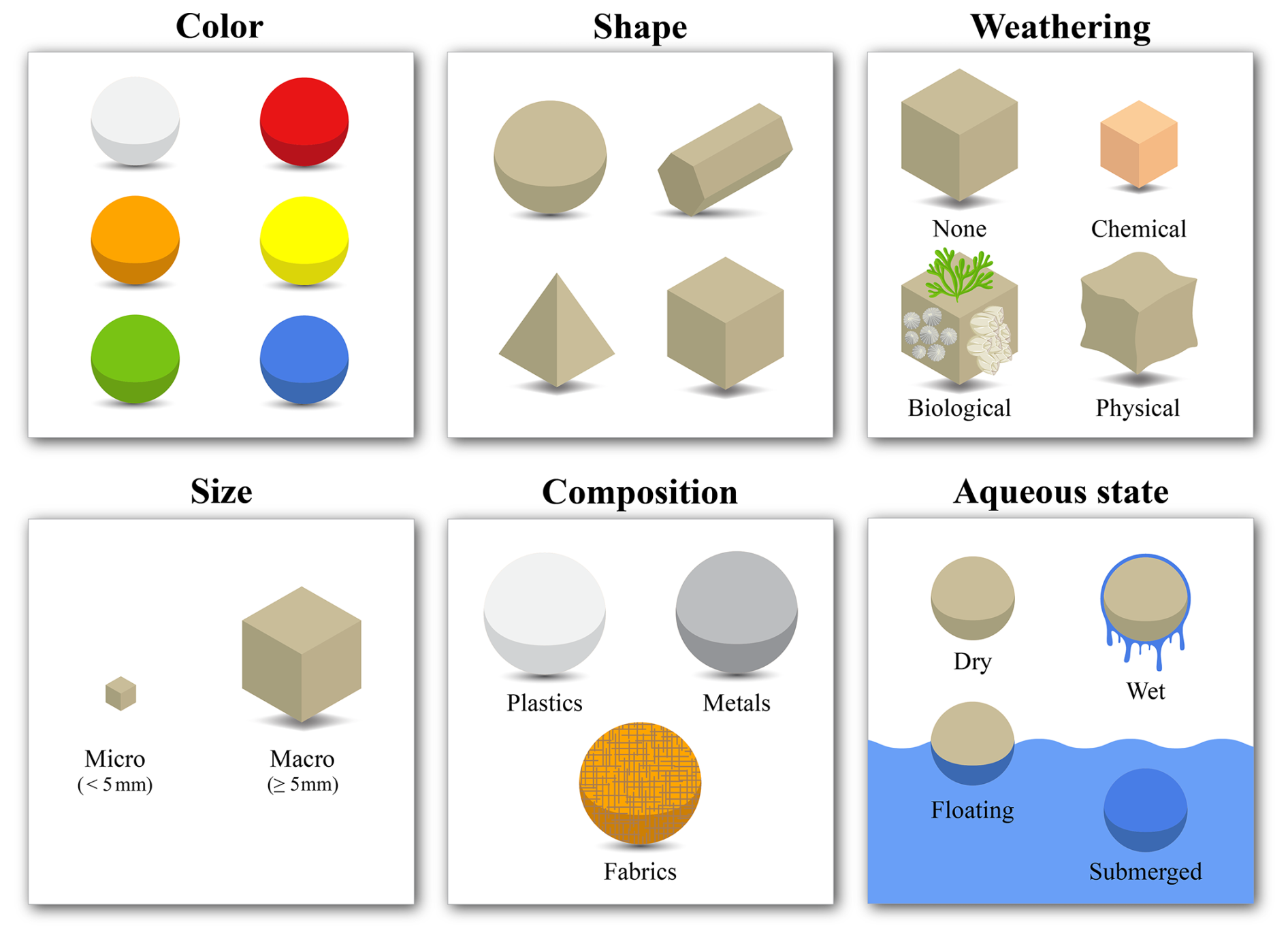
Remote sensing has the potential to support the monitoring of aquatic debris concentrations and dispersal patterns across spatial and temporal scales. From this perspective, the definition of marine debris is broadened to include not only anthropogenic materials, but also natural materials such as algal patches, wood, pollen, pumice or seaweed species (Martínez-Vicente et al., 2019; Maximenko et al., 2019; NASEM, 2021; Hu et al., 2023; Garaba et al., 2023). However, ongoing efforts in remote sensing of marine debris are challenging due to the complexity of the targets (de Vries et al., 2023a; NASEM, 2021; GIZ, 2023). Debris objects vary widely in physical properties (e.g., color, shape, composition, size) that are further influenced by environmental factors such as aqueous state and stage of weathering (Fig. 1). Fully understanding marine debris diagnostic optical properties is essential for building, training, and validating remote sensing detection algorithms (Garaba et al., 2021a; Garaba and Harmel, 2022). This information, together with the evolution of hyperspectral remote sensing technologies and the development of active and passive sensors, is expected to further advance current capabilities to detect and monitor marine debris.

Figure 1 Examples of physical and chemical characteristics of marine debris in nature.

The reflectance parameter is one of the common remote sensing parameters that describes the ratio of light reflected off an optically active sample with respect to a known standard like a Lambertian equivalent target. Reflectance measurements, when collected under controlled conditions using instruments such as handheld spectroradiometers, minimize the environmental variability, which is ideal for initial algorithm development (Knaeps et al., 2021; de Vries et al., 2023a; Garaba et al., 2021a, 2020a). Recent stakeholder discussions facilitated by the International Ocean Colour Coordinating Group Task Force on Remote Sensing of Marine Litter and Debris highlighted the need for a comprehensive, well-curated spectral reference library (SRL) of marine debris reflectance. SRLs support algorithm development by offering spectral data of known objects, establishing a baseline database that can be used to identify unknown objects. However, current marine debris reflectance datasets have been gathered using variable methodologies, data processing, and metadata curation, making it challenging to combine them for algorithm development and to identify gaps in the field.

In this study, we leverage the wealth of available spectral reflectance measurements of marine debris to build a consistent and extensive collection. We compiled, assessed, and curated the available marine debris reflectance datasets into a single SRL called the MArine Debris hyperspectral reference Library collection (MADLib). MADLib aims to improve the accessibility and comparability of current data to promote the spectral exploration and analysis needed for marine debris algorithm development. We also aimed to follow the FAIR guidelines by making the data findable, accessible, interoperable, and reusable (Wilkinson et al., 2016). Here, we explain how the data contained in the collection was curated, identify existing sampling gaps, and discuss factors that are important for the trustworthiness of future SRLs and remote sensing of marine debris.

2 Methods and materials

2.1 Selection of datasets

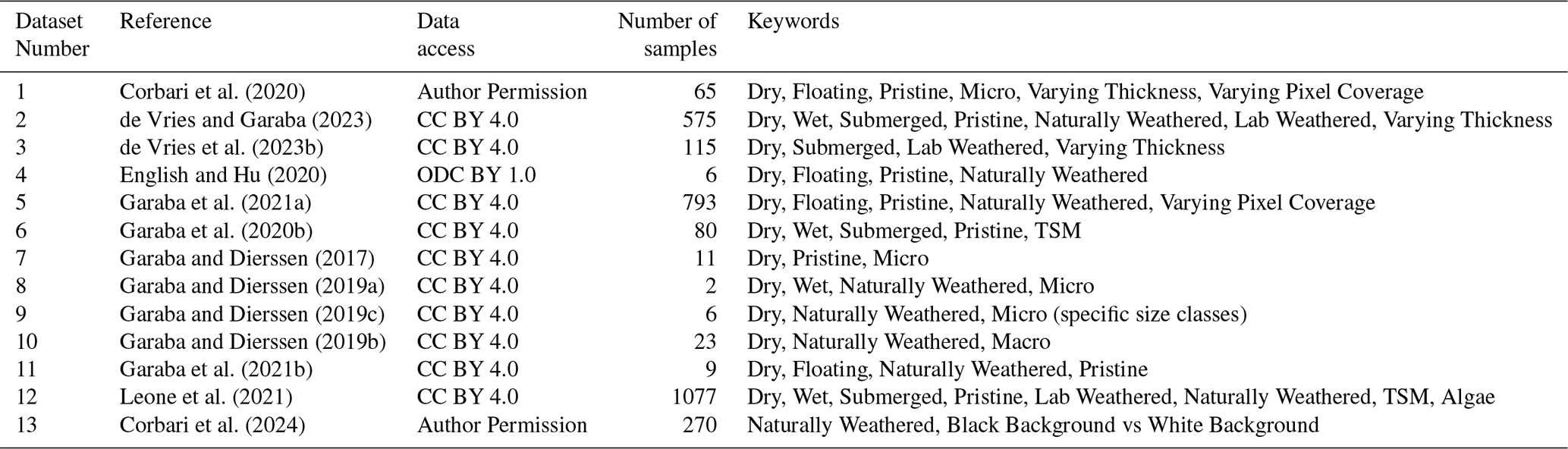
Thirteen datasets were selected for curation and creation of MADLib collection from open-access sources as well as upon request from authors (Table 1). The selected datasets had the following characteristics (i) the data reported were relative reflectance not remote sensing reflectance, (ii) reflectance was measured using a handheld spectroradiometer, and (iii) hyperspectral data were provided in the visible to shortwave infrared (SWIR) region. The remaining datasets found in the literature either did not meet these criteria, were not readily available upon request, or needed further curation from the authors (e.g., Acuña-Ruz and Mattar, 2020; Olyaei et al., 2024; Tasseron et al., 2021; Wang et al., 2024; Knaeps et al., 2020). Leveraging the datasets (Table 1), we determined a standard formatting structure from which to build the MADLib collection. This included several spectral data processing steps for quality control (Sect. 2.3) and gathering additional metadata parameters about the samples (Sect. 2.4).

Table 1 Source of hyperspectral measurements used to create MADLib.

2.2 Materials

MADLib includes 3032 samples compiled from thirteen datasets (Table 1). Each sample represents either a single marine debris object (e.g., a bottle, buoy) or an assemblage of micro-sized items (e.g., a collection of microplastic particles measured together) measured under specific conditions. For example, the same object measured in both dry and submerged states was represented as two separate samples in MADLib. Each sample is associated with a spectrum and the related metadata. The samples encompass a wide variety of colors, sizes, polymer types, weathering conditions, aqueous states, and experimental designs. It should be noted that, while these datasets include various debris types, plastic is the dominating type of debris reported, reflecting its overwhelming presence in the marine environment.

2.3 Spectral data processing

Each dataset was downloaded from its respective open-access platform or requested from the corresponding author and assembled into MADLib. Spectral reflectance measurements covered a wavelength range between 280–2500 nm with 1 nm resolution. In most cases, multiple spectral measurements were recorded per sample, sometimes in various geometric orientations. We will refer to these measurements as replicates, which account for within-sample variability and instrument noise.

The final MADLib spectral data download includes five identification columns: dataset number, sample number, data type, replicates and flags. Dataset number refers to the cited datasets (Table 1). Sample number uniquely identifies each sample within a specific dataset. Data type specifies whether the data in that row represents the “mean”, “median”, or standard deviation “stdev” of that sample's replicates, or “single” for single measurements without replicates. Replicates provides the number of replicates associated with that statistical representation. The Flags column contains a “1” for spectra containing more than 50 % NaN values and otherwise contains a “0”. The data are sorted alphanumerically by data type, then dataset number, and finally sample number.

2.3.1 Data formatting

Spectral data were obtained in one of four formats depending on the dataset: (1) individual spectral measurements for each replicate, (2) pre-calculated means, medians, and standard deviations of the replicates per sample, (3) only the mean spectral reflectance values of the replicates per sample, or (4) single reflectance measurements per sample without replicates.

When more than one individual spectral measurement per sample was provided, the mean, median, and standard deviation of the replicate measurements were calculated for each sample to standardize across datasets. Two datasets provided only mean spectral reflectance values of their sample's replicate measurements, so the median and standard deviation for these data were written as NaNs (Not a Number) in MADLib. Single measurements were provided for six samples across three datasets and were classified separately as “single”.

MADLib only reports the descriptive statistics of the compiled data as mean, median and standard deviation of the replicates (with the two exceptions specified above). In total, MADLib summarizes the information from 24 889 replicate measurements of 3032 samples collected from thirteen datasets (Fig. 2). In the datasheet, 3026 mean measurements, 2691 median measurements, and 2691 standard deviation measurements are recorded. Six samples did not have replicates, so they are available as individual measurements without summary statistics.

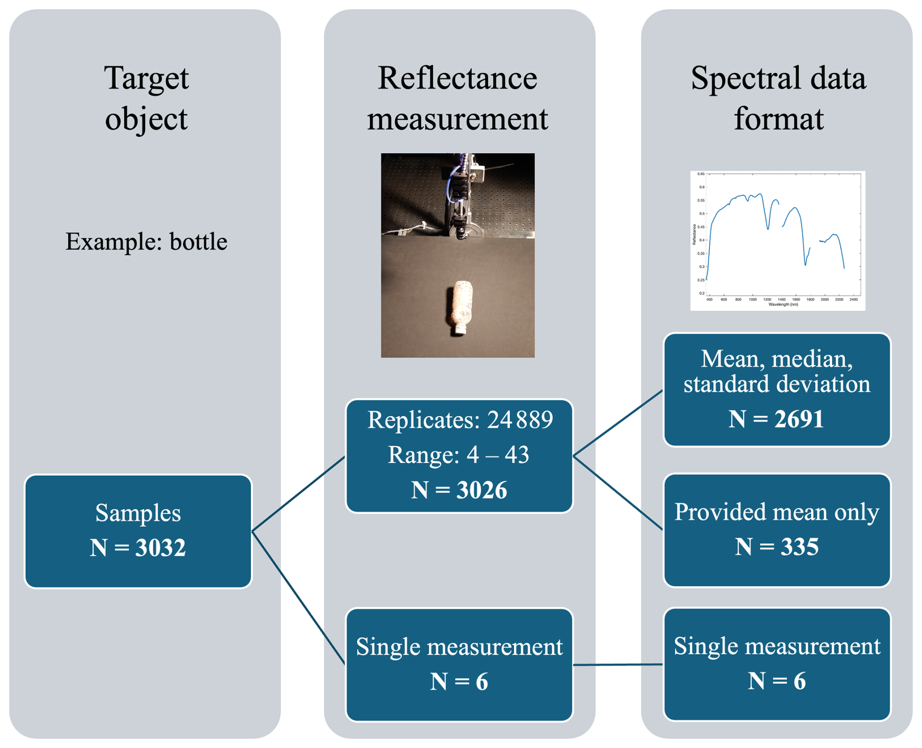
Figure 2 Breakdown of the number of samples, replicate measurements for total samples, and descriptive statistics of sample spectra within MADLib.

2.3.2 Wavelength range adjustment

A wavelength range limit of 280–2500 nm was applied to ensure consistency across datasets. NaNs were used in place of the missing spectral data for instruments not collecting data in the fixed range.

Splice correction

Hyperspectral instruments measuring beyond the visible-near-infrared (VNIR, 280–1000 nm) consist of multiple detectors, each covering a distinct spectral range. Off-the-shelf spectroradiometers commonly used in environmental remote sensing applications (e.g., Analytical Spectral Devices FieldSpec 4, Spectral Evolution SR-3501, Spectral Evolution SR-1901) have three detectors. When transitioning between the detectors, slight differences in sensitivity, temperature or calibration can create discontinuities in the reflectance spectral measurements. The spectral discontinuities, or “steps”, usually occur around 1000–1001 and 1800–1801 nm, but the exact positions are instrument and manufacturer specific (Fig. 3a, e, f). The spectral data from each dataset were visually inspected for steps. If a step was identified, we calculated the linear difference at each step and adjusted one region of the spectrum based on another to eliminate the gap (Garaba et al., 2021a). The middle detector (1000–1800 nm) was considered as the reference, and the adjacent regions (280–1000 and 1800–2500 nm) were adjusted to that reference level. For example, if the reflectance difference between 1000 nm and 1001 nm is −0.02, then 0.02 is subtracted from all values in the 280–1000 nm range to align it with the more stable middle region (Fig. 3b).

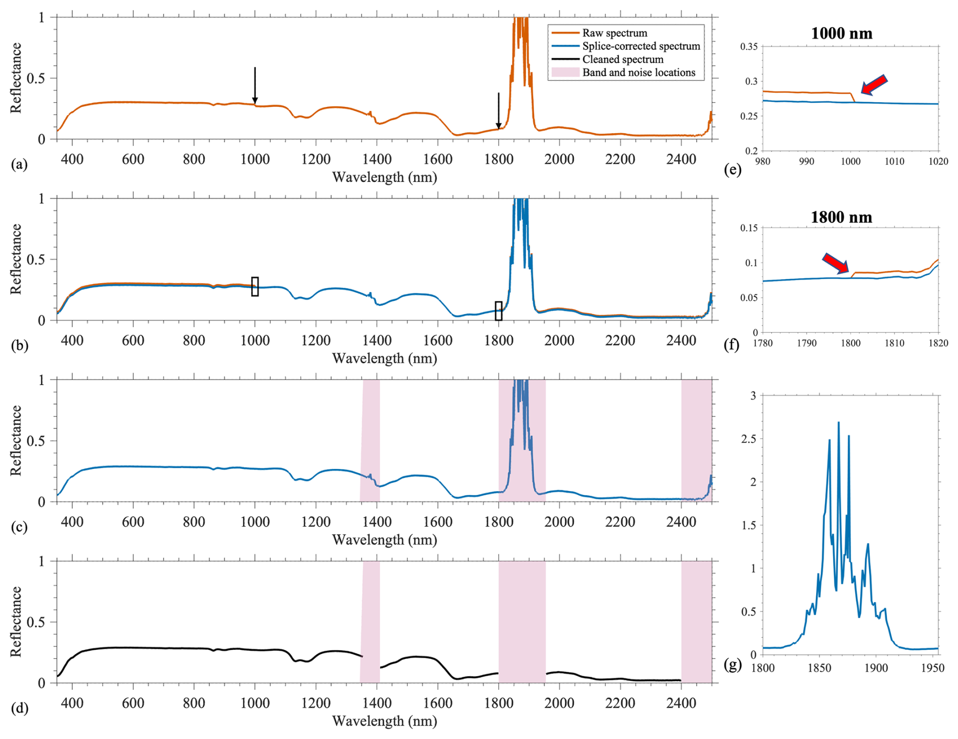
Figure 3 Example processing steps for spectra: (a) raw downloaded spectrum; (b) comparison of raw and splice-corrected spectra, (c) identification of atmospheric absorption bands and instrument noise; and (d) final cleaned spectrum. (e) Zoom-in of the 980–1020 nm region in (b), highlighting the splice correction at 1000 nm. (f) Zoom-in of the 1780–1820 nm region in (b), highlighting the splice correction at 1800 nm. (g) Zoom-in of the 1800–1950 nm region in (d), showing the full reflectance magnitude of the atmospheric absorption band.

2.3.3 Noise removal

Visual inspection was used to identify, and subsequently remove, noise in the spectra. The affected wavelengths were replaced with NaNs to avoid misinterpreting them as real spectral features in later analyses (Fig. 3d, g). Noise was considered to arise from two main sources: atmospheric absorption bands and instrument-related noise. Strong atmospheric absorption occurs in the SWIR, specifically around 1350–1450, 1800–1950, and above 2400 nm (Garaba and Dierssen, 2020; Clark et al., 2003). This effect is observed in outdoor measurements, where sunlight interacts with larger portions of the atmosphere before reaching the sample. Spectra often exhibit abrupt, isolated peaks due to these atmospheric absorption bands. Instrument noise was also observed, particularly at the extreme ends of the spectral range, where sensor sensitivity tends to decrease.

2.3.4 Flags

Hyperspectral data (mean, median, standard deviation, or single measurement) with more than 50 % NaN values across the original wavelength range were flagged. The flagged entries were kept in MADLib for completeness but were marked with an additional “flags” column to indicate data quality. A binary code of “1” indicates a flagged sample, while “0” indicates a clean sample.

2.4 Metadata curation

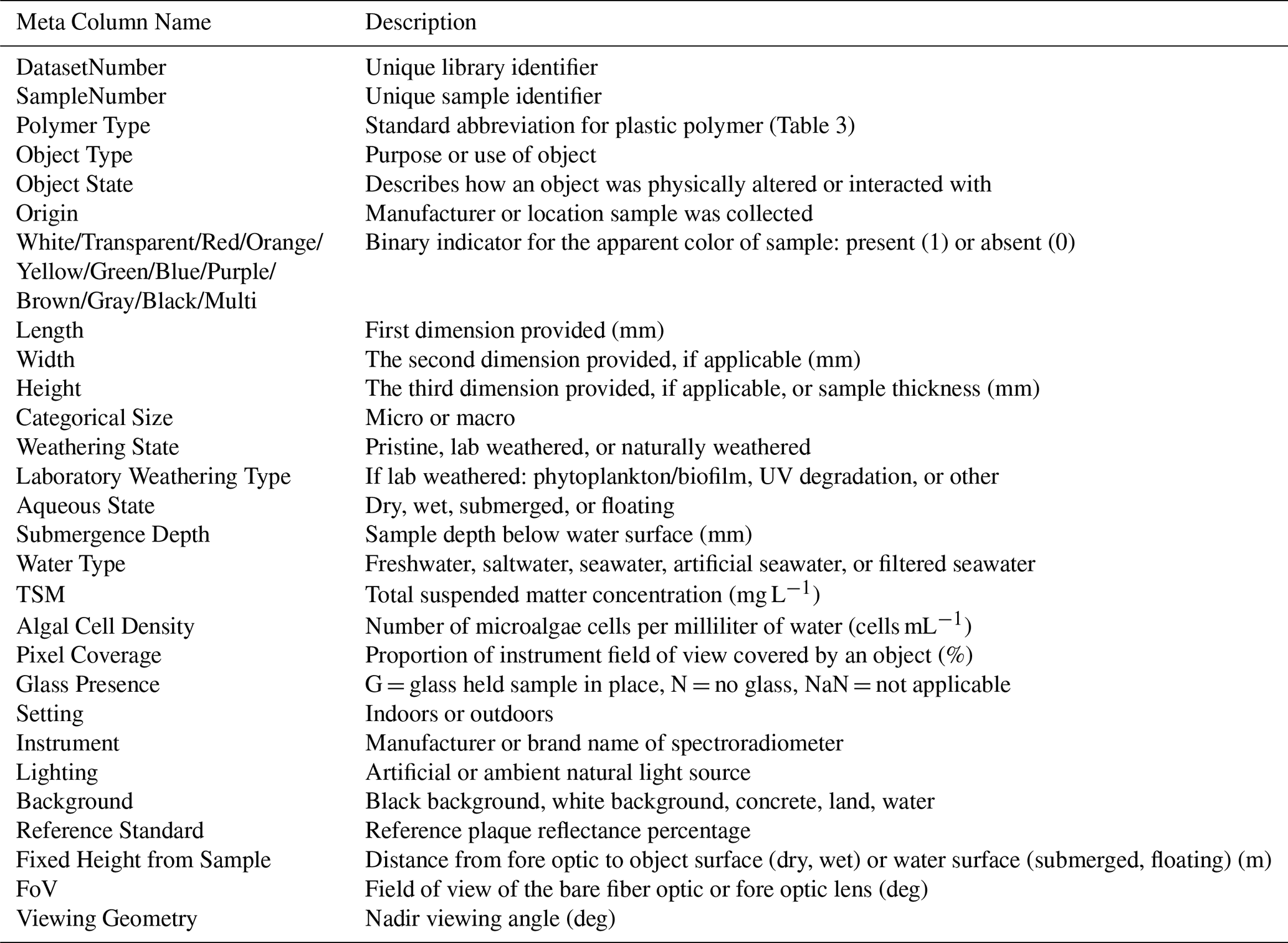
MADLib incorporates the unique metadata provided for samples from each dataset, adds new metadata parameters, and ultimately provides comprehensive metadata descriptors for improved interoperability. Metadata descriptors date/time, longitude, latitude, FTIR identification, and sample weight were excluded from the curation due to their limited applicability across datasets and the potential for misleading interpretation since the samples were not imaged in situ. Metadata were incorporated from existing metadata files, descriptions within associated publications, and, when necessary, missing details were obtained from the authors directly. When this was not possible, NaN values were assigned to indicate the missing metadata. The final MADLib metadata download includes thirty-nine columns of metadata descriptors (Table 2). The thorough curation process in MADLib enabled more detailed and robust analyses, focusing on parameters that enhance the identification and classification of marine debris through reflectance measurements.

Table 2 List of MADLib metadata descriptors.

2.4.1 Sample type

Despite MADLib containing a variety of marine debris types, it is primarily composed of plastic debris. Consequently, this paper will address plastic-specific characteristics, such as polymer type, in addition to broader characteristics. Sample type parameters included polymer type, object type, object state, and origin to maximize dataset comparability. For example, if a dataset described a sample as “crushed PET water bottle”, we further described it using polymer type = “PET”, object type = “bottle”, and object state = “crushed”. During this process, the polymer type, object type, and object state were simplified or modified to ensure consistency and comparability across datasets. For example, object types labeled as “water bottle”, “clear water bottle”, “bottle”, “plastic bottle”, or any similar terminology were all simplified to “bottle”. Origin was provided if the dataset specified the manufacturer or place the item was retrieved from.

2.4.2 Color

Colors are categorized as white, transparent, red, orange, yellow, green, blue, purple, brown, gray, black, and multi to ensure consistency and comparability across samples. For example, pre-existing samples marked as tan, dark brown, light brown, and brown were all included in the brown category. Colors were recorded with binary entries to easily identify objects with multiple colors. If more than one color was specified by the original author, all relevant colors were marked with a 1. If multi-colored was specified by the original author, only multi was marked with a 1.

2.4.3 Size

Object dimensions were recorded differently across datasets and required representation in various formats. The length, width, and height columns were used for objects with complete dimensional data, while the height column additionally represented thickness where relevant. If a range of sizes was provided (e.g., 1–3 mm) by the authors of the original dataset, then the average was included (e.g., 2 mm) in MADLib. If a height or thickness smaller than 1 mm was provided, then 1 mm was reported. In some cases, the authors alternatively provided categorical size data, either “micro” (< 5 mm) or “macro” (> 5 mm), so we included a categorical size classification. Samples with numerical data provided were categorized as “micro” if all three dimensions (L, W, H) were less than 5 mm. If only partial size data were available and under 5 mm, samples were not categorized as “micro” to avoid errors in cases where a missing dimension might exceed 5 mm. Conversely, any sample with one or more dimensions more than 5 mm was classified as “macro”.

2.4.4 Weathering

Weathering state was specified as either “pristine”, indicating non-weathered, virgin material; “lab weathered”, subjected to controlled laboratory conditions; or “naturally weathered”, collected from the marine environment and exposed to natural processes. The specific type of lab weathering was indicated as either “biofouled” or “UV exposure” in the lab weathering type metadata column. Samples labeled as “biofouled” were submerged in natural water within a mesocosm to promote biofilm growth (de Vries et al., 2023b; Leone et al., 2021). Some of these samples were additionally labeled as rough if their surfaces had been abraded with sandpaper prior to submersion (Leone et al., 2023). To simulate photodegradation, other samples were exposed to ultraviolet (UV) radiation under either dry or wet conditions (Leone et al., 2023).

2.4.5 Aqueous state and water properties

Four categories describe the aqueous state of the samples: “dry”, “floating”, “submerged”, and “wet”. “Dry” samples refer to dry objects measured on a dry surface. “Wet” samples refer to wet objects measured on a dry surface or above a water body. “Floating” samples refer to any object floating on the surface of a water body or in a water tank. “Submerged” samples refer to any object where the top is at least 1 mm under the water's surface.

If the sample was categorized as “wet”, “floating”, or “submerged”, and information on the properties of the water in which it was measured were available, they were also included. Water type specifies if the sample was measured in “freshwater”, “saltwater”, “seawater” (unfiltered), “artificial seawater”, or “filtered seawater”. In some cases, samples were measured in a mesocosm or water bath that had added total suspended matter (TSM) or phytoplankton (Leone et al., 2021; Garaba et al., 2020b). Concentrations were included in TSM and algal cell density columns. Additionally, the submergence depth of samples in millimeters under the water surface was provided in the submergence depth (mm) column, ranging from 5 to 715 mm.

2.4.6 Experimental setup

The location of measurement, setting, was categorized as “indoors” or “outdoors” for all samples. Lighting was similarly categorized for each location, with indoors using tungsten halogen lamps, or outdoors using sunlight with recorded conditions (Fig. 4). Studies also varied with the viewing geometry, field of view (FoV), and fixed height from sample. Dry surface and water bath samples were measured on a black background with the exception of one dataset which used both black and white backgrounds for comparison (Corbari et al., 2024).

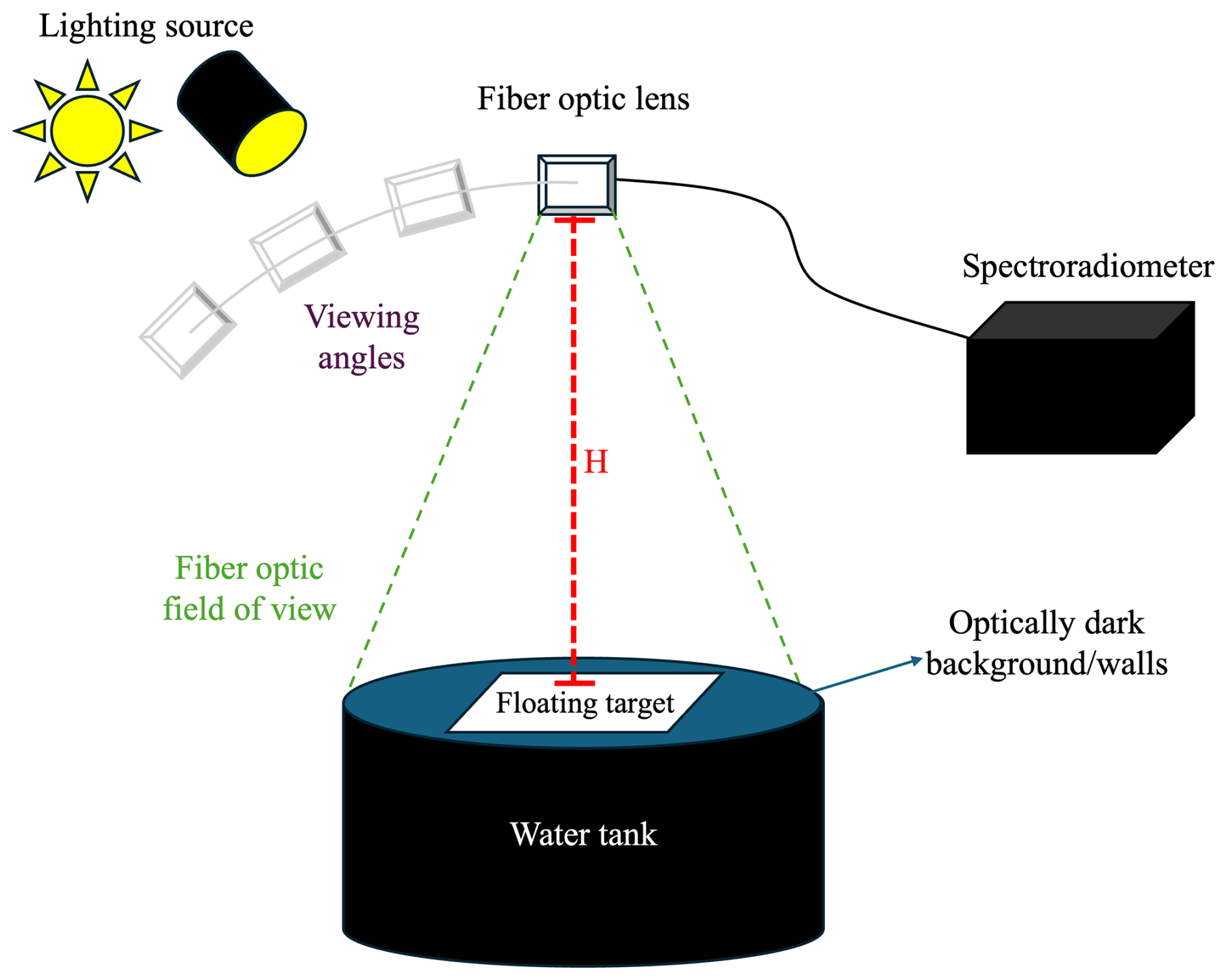
Figure 4 Schematic of typical experimental setup with the light source, variable viewing geometry, fiber optic field of view, fixed height from sample (H), and an optically dark background.

Other controlled sample parameters included Pixel Coverage and Glass Presence. Pixel Coverage, also referred to as areal fractional cover, refers to the percentage of the field of view containing the sample and was used to measure varying concentrations of plastics (Garaba et al., 2021a; Corbari et al., 2020). Glass was used in one dataset to hold samples in place, therefore causing a possible disruption to the produced spectra (de Vries and Garaba, 2023). Further information on protocols specific to each dataset may be found in the original publications (Corbari et al., 2024, 2020; de Vries et al., 2023a; English and Hu, 2020; Garaba and Dierssen, 2020; Knaeps et al., 2021; Garaba et al., 2021a, b; Leone et al., 2023).

3 Results

Here, we examine the distributions of several characteristics within MADLib and present case studies of spectral reflectance where relevant. To ensure consistency, all spectra plotted in this study correspond to the mean of replicate measurements for each sample.

3.1 Polymer type

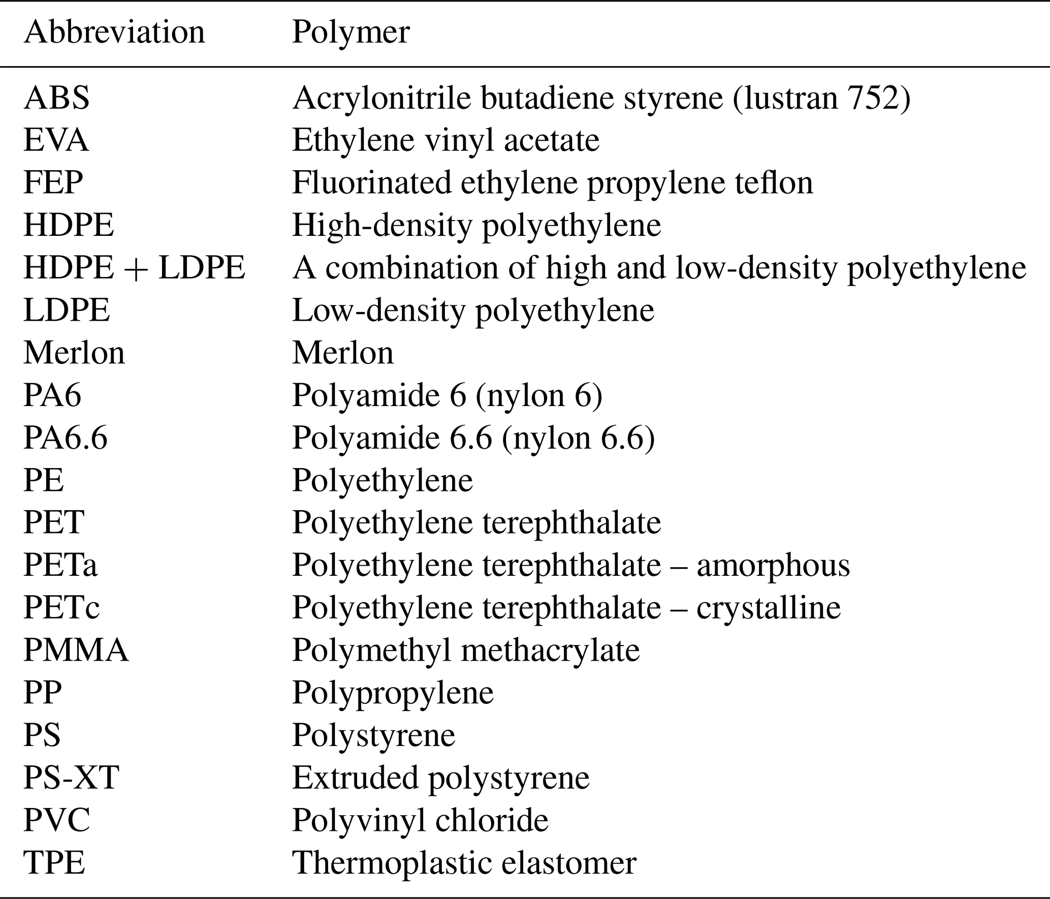
Nineteen distinct polymer types are included in the dataset (Table 3). The largest group of samples are of an unknown polymer type (35 %) (Fig. 5a). The unknown polymer category includes plastics with unidentified polymer types as well as non-plastic marine debris, such as fabrics, metals, and background materials. Polypropylene (PP) is the most common polymer type, making up 15 % of the samples, followed by polystyrene (PS) and high-density polyethylene (HDPE) (Fig. 5a). Only one sample is available for each of the following six polymers: terpolymer lustran 752 (ABS), fluorinated ethylene propylene teflon (FEP), merlon, polyamide 6.6 (PA6.6), polymethyl methacrylate (PMMA) and thermoplastic elastomer (TPE). Some polymer types in MADLib exhibit similar spectral features across the NIR–SWIR range, while others display distinct or minimal spectral features (Fig. 5b).

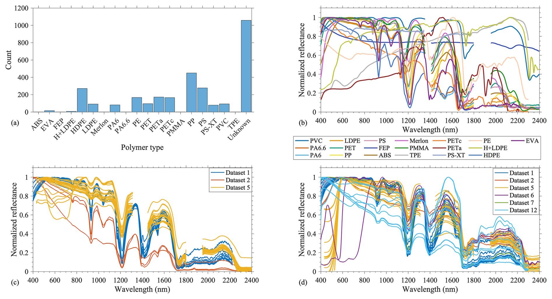
Figure 5 (a) Distribution of polymer types; (b) example reflectance spectra for each polymer type in MADLib; (c) reflectance spectra of all available pristine and dry HDPE samples; and (d) reflectance spectra of all available pristine and dry PP samples. Each reflectance spectrum was normalized to its own maximum reflectance value.

The reflectance spectra of all pristine, dry PP and HDPE samples are isolated and presented separately to inspect intra-variability in spectral features of measured polymers (Fig. 5c, d). These polymers were selected because they are well represented in MADLib, with numerous samples originating from several independent datasets. The spectral shape in the visible spectrum is consistent with the apparent color of each object; this is further explored in Sect. 3.3. In the case of the PP samples, the objects in dataset 6 were observed to be transparent, orange, and blue in color, while those in datasets 1 and 7 were white/transparent, those in dataset 2 were grey, and those in dataset 5 were yellow and brown (Fig. 5d). Dataset 12 did not provide information on apparent color. The absorption features within the SWIR are consistent across samples of the same polymer type and align closely with reported literature (Olyaei et al., 2024; Garaba and Dierssen, 2020). The observed differences in magnitude between spectra from a single dataset are associated with changes in sample thickness and size (datasets 1, 2, and 12), glass presence (dataset 2), or pixel coverage (dataset 5). Measurements between datasets also differed in acquisition, such as fiber optic field of view and height of instrument from sample at time of measurement, which may affect pixel coverage.

Table 3 Standard abbreviations of polymer types in MADLib.

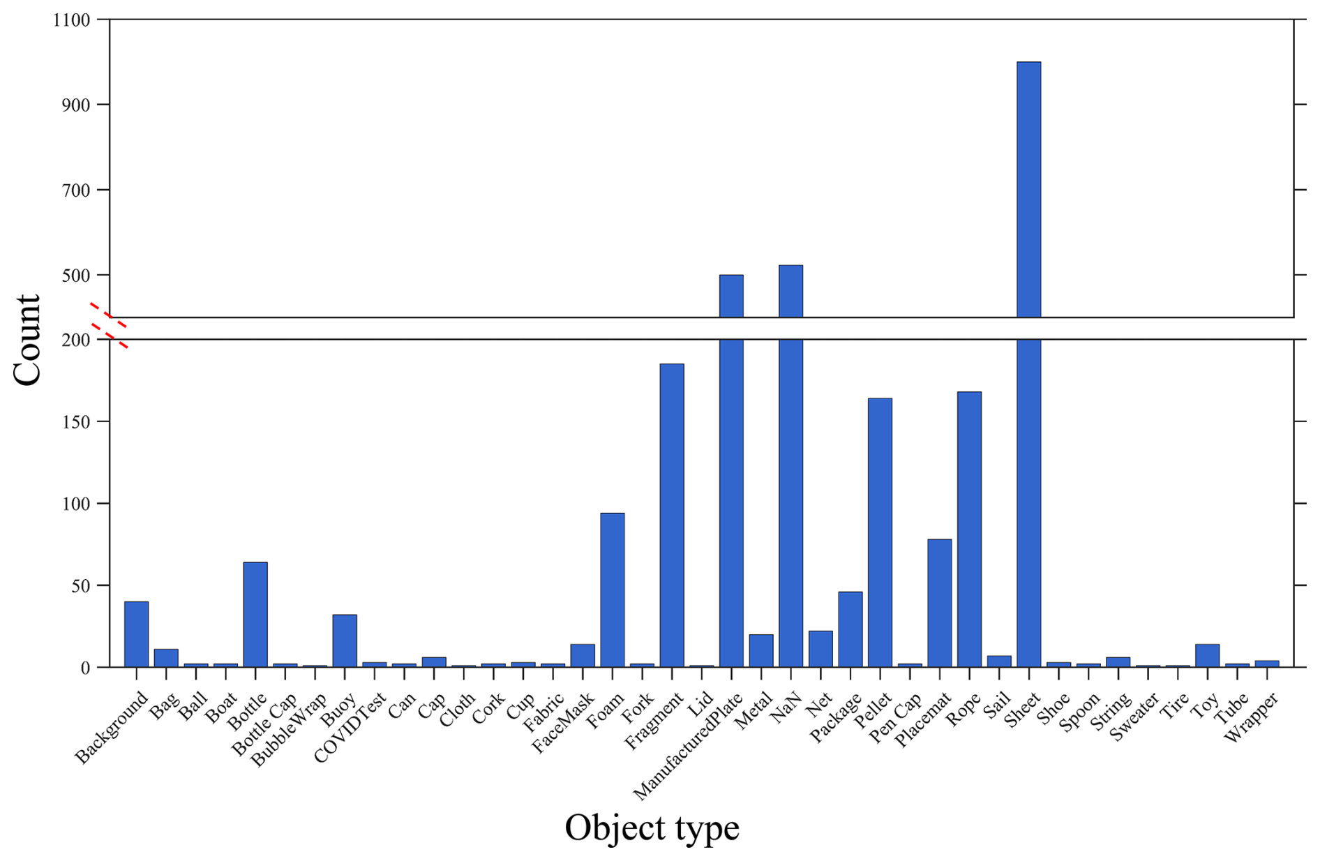
3.2 Object type

Thirty-nine object types are used to define the samples, noting that 17 % of samples are of unknown object type (Fig. 6). Among those that could be classified, the top two categories are sheet (33 %) and manufactured plate (16 %). We note that the majority (88 %) of samples labeled as sheet and all samples labeled as manufactured plate were obtained directly from the manufacturer as a single polymer composition. There are five object types (bubble wrap, cloth, lid, sweater, and tire) for which only one sample was measured.

Figure 6 Distribution of object types among samples in MADLib.

3.3 Color

Twelve color categories are used in MADLib. The three largest categories are unspecified (30 %), white (19 %), and grey (15 %) (Fig. 7a). The categories brown, black, blue, and transparent contain approximately 5 %–8 % of the total samples each. 16 % of the samples are categorized as having more than one color.

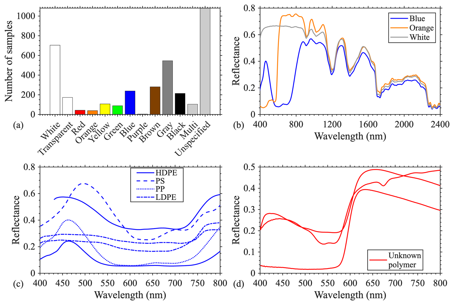
Figure 7 (a) Distribution of sample colors within MADLib, (b) reflectance spectra of the same polymer and object (polypropylene placemat) in three different colors (c) six blue colored samples of different polymer types, and (d) three red samples of unknown polymer type.

As expected, when color is isolated as the only changing characteristic, it most significantly influences the visible region of the spectrum (400–700 nm). For instance, blue-colored objects exhibit a reflectance peak near 470 nm, while white-colored objects show consistently high reflectance across the visible range (Fig. 7b). In the NIR–SWIR region, absorption features associated with polymer type remain unchanged regardless of color. When different polymer types of the same color are compared, similar peaks exist in the visible region, as expected, with some minor variations (Fig. 7c–d).

3.4 Size

Using the available quantitative and qualitative size data, all samples are categorized as macro, micro or uncategorized due to a lack of available size data. Nearly half (41 %) of the samples within the dataset are unable to be categorized (Fig. 8a). Of those categorized, the majority (90 %) are considered macro-sized, and only 10 % are micro-sized. Our results show that the locations of absorption features within the SWIR are consistent for micro- and macro-sized debris of the same polymer types (Fig. 8b–d). In each example, the microplastic and macro-plastic measurements are from different datasets (Fig. 8b–d). Therefore, there are differences in sample color as well as experimental setup (such as field of view or height of spectroradiometer from sample) between the two samples. Differences in spectral features within the visible region are likely due to color inferred from the corresponding peaks. Other slight differences in feature location may be attributed to other metadata (e.g., additives, state of weathering, etc.). Additionally, we note that the HDPE microplastic spectrum has a pixel coverage of 90 %, compared to 100 % for all other spectra.

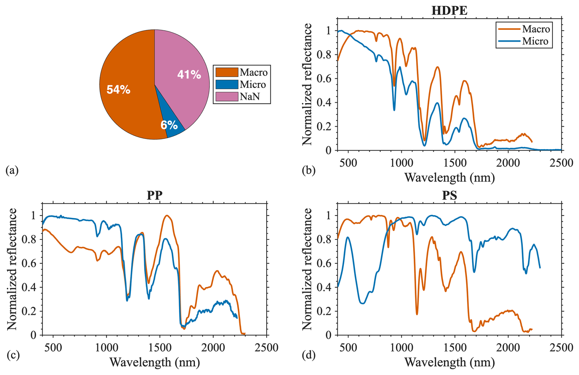
Figure 8 (a) Categorical size distribution of samples within MADLib; and (b–d) example reflectance spectra of micro- and macro-sized (b) HDPE (c) PP, and (d) PS. Each reflectance spectrum was normalized to its own maximum reflectance value.

3.5 Weathering state

The three categories of weathering – pristine, lab weathered and naturally weathered – have relatively equal contributions to the curated dataset, with less than one percent of samples left undefined (Fig. 9a).

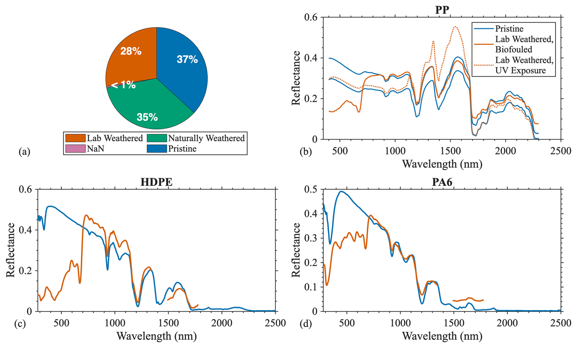
Figure 9 (a) Distribution of weathering state categories within MADLib; and (b–d) example reflectance spectra for pristine and lab-weathered (biofouled or UV-exposed) samples: (b) PP, (c) HDPE, and (d) PA6.

Case studies of three polymer types (PP, HDPE, and PA6) are presented before and after lab weathering (Fig. 9b–d). Naturally weathered samples are not compared in the case study because no samples were measured before and after natural weathering for comparison. The two types of lab weathering, biofouling and UV exposure, produce different effects on reflectance within the visible spectrum. Samples exposed to UV radiation (dotted orange line) follow similar trends to their pristine counterparts with elevated reflectance values within the 1200–1600 nm range (Fig. 9b). In comparison, all biofouled samples (solid orange lines) show reduced reflectance across the visible spectrum and exhibit a pronounced chlorophyll-a absorption feature at 670 nm (de Vries et al., 2023a) (Fig. 9b–d). No major spectral shape differences are found in the NIR-SWIR region before and after biofouling; all the major spectral features for each polymer type remain the same.

3.6 Aqueous state

In MADLib, submerged samples constitute the largest aqueous state category (43 %), followed by dry samples (35 %), with fewer classified as floating (14 %) or wet (8 %) (Fig. 10a). Each submerged object was measured at 3–20 separate depths to assess the effect of depth on spectral features, influencing the overall distribution. Less than one percent of samples is missing an aqueous state classification.

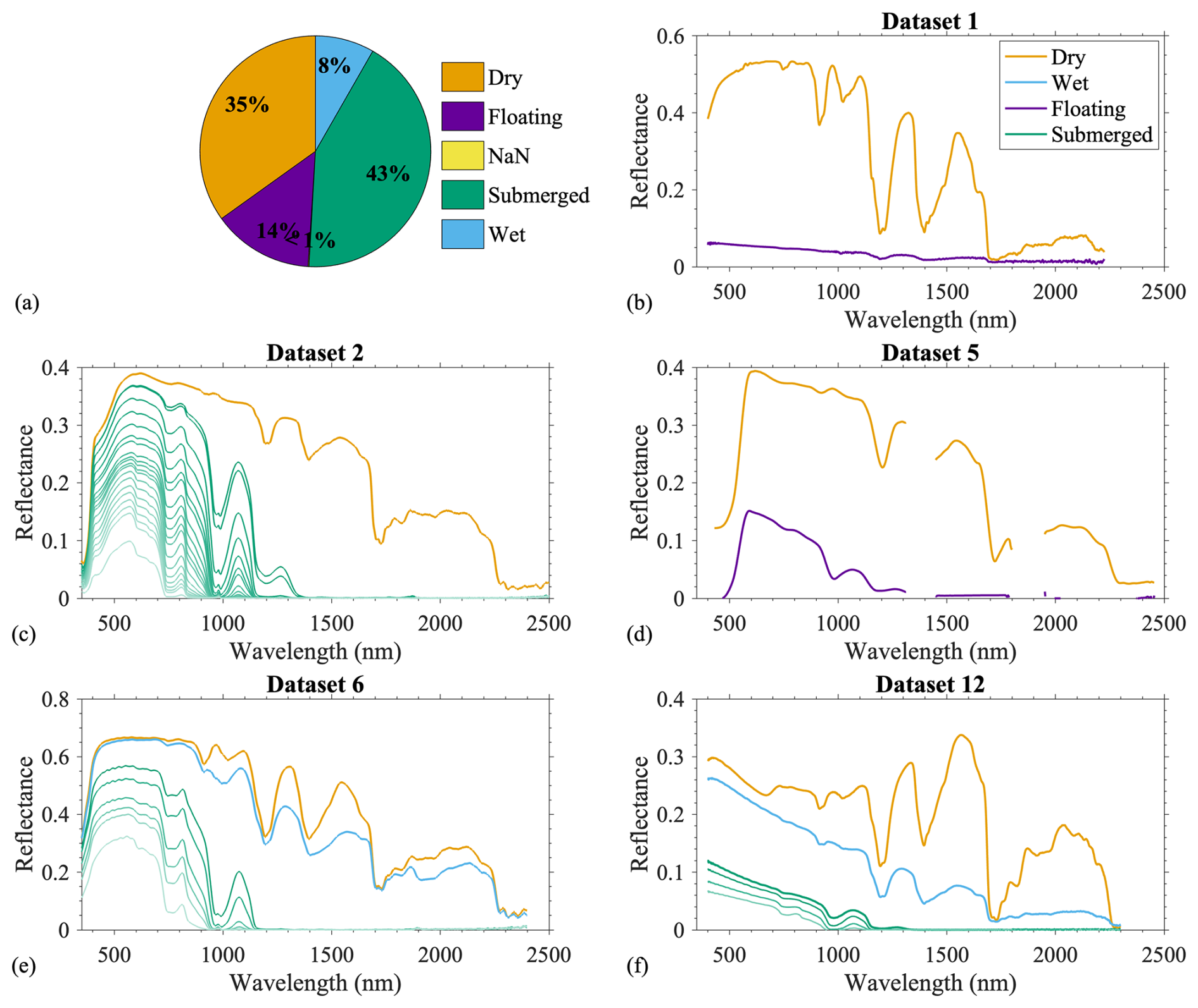
Figure 10 (a) Distribution of aqueous state categories within MADLib; and (b–d) example reflectance spectra of dry polypropylene across four aqueous state categories, using datasets (b) 1 (dry and floating), (c) 2 (dry and submerged), (d) 5 (dry and floating), (e) 6 (dry, wet, and floating), and (f) 12 (dry, wet, and floating). Submerged samples (c, e, f) are shown at depths ranging from 5 to 715 mm.

To examine the effect of the aqueous state on reflectance, a case study on the mean reflectance of pristine polypropylene samples from several datasets is presented. Reflectance magnitude decreases with increasing water interference in all cases, being highest for dry samples, followed by wet and floating/submerged samples. The case study reveals consistent spectral features in dry polypropylene across all four datasets (Fig. 10b–e). The same spectral features are present for wet polypropylene samples as well (Fig. 10e–f), but not present in submerged samples (Fig. 10c, e, f). All submerged samples lose signal in the SWIR and their reflectance magnitudes decrease as depth increases (Fig. A1), both of which are expected due to water's high absorption in the IR (Garaba and Dierssen, 2020). Submerged samples exhibit unique peaks at approximately 810 and 1070 nm, which are consistent across datasets (Fig. 10c, e, f) and polymer types (Fig. A1). The floating objects represented from datasets 1 and 5 have pixel coverages of 66 % and 60 %, respectively, representing the highest available pixel coverage for dataset 1 and the closest match for dataset 5 (Fig. 10b, d). The dataset 1 sample exhibits the same prominent SWIR absorption features when dry and wet, while the reflectance shape of the dataset 5 floating sample more closely resembles a submerged debris item (Fig. A2). The reflectance shape in the visible region is related to object color in both cases. Both floating measurements have more noise and missing values in the infrared than the dry measurements.

4 Discussion

The analysis of MADLib revealed distinct spectral features linked to various characteristics of debris, as well as key gaps in available data. Below, we interpret these findings, highlight MADLib's utility and limitations, and offer recommendations for future data collection and research directions.

4.1 Preliminary lessons from MADLib

MADLib offers a valuable and improved starting point for the development of algorithms aimed at detecting marine debris, particularly plastics. Preliminary analyses highlight the role of apparent color and biofilm presence on spectral shape in the visible spectrum (Figs. 7b, 9b), whereas polymer type and aqueous state more strongly affect spectral shape in the SWIR region (Figs. 5b, 10b–f). Previous studies have also found apparent color to influence spectral shape and magnitude in the visible spectrum, while the SWIR region remains largely unaffected regardless of the intrinsic color of the object (Knaeps et al., 2021; Garaba et al., 2021a). Biofouling of plastics has similar results, with the SWIR properties remaining largely unchanged, while spectral shape and magnitude are altered in the visible spectrum exhibiting a pronounced red edge feature (de Vries et al., 2023a). Measurements of wet, floating, and submerged debris show reduction in magnitude across the spectrum, especially in the SWIR, compared to dry debris (Knaeps et al., 2021; Garaba et al., 2021a; de Vries et al., 2023a). Submerged objects have minimal signal in the NIR-SWIR compared to other aqueous states and unique spectral features in the NIR near 810 and 1070 nm (Knaeps et al., 2021; de Vries et al., 2023a). Distinct spectral differences between submerged plastics and other aqueous states (Fig. 10c, e, f) suggest that separate detection algorithms may be required for submerged debris using the visible or NIR spectral regions. Given the limited polymer-specific features within the visible range, we further recommend focusing on SWIR wavelengths for algorithm development of non-submerged debris as prior studies have suggested (Garaba and Harmel, 2022). Several studies have demonstrated prospective plastic detection using high-resolution sensors with appropriate SWIR spectral bands (Guo and Li, 2020; Asadzadeh and Filho, 2016; Park et al., 2021; Kremezi et al., 2021), suggesting that prioritizing future sensors with appropriate spatial resolution (e.g., 30 m or less) and band placement could make SWIR-based approaches viable.

Although MADLib includes many samples categorized under the same polymer type and aqueous state, no two samples are identical. Every sample differs by at least one physical property or measurement condition, creating both challenges and opportunities. On one hand, polymer type comparisons (e.g., among polypropylene samples) may be confounded by variation within other sample characteristics, environmental perturbations, or experimental design (Fig. 5c, d). On the other hand, this heterogeneity mirrors real-world conditions and provides a chance to identify robust spectral features that persist across variability. In this way, the breadth of measurement conditions available in MADLib can serve as a testing ground for existing plastic detection algorithms (Asadzadeh and Filho, 2017; Kühn et al., 2004; Zhang et al., 2022; Guo and Li, 2020; Garaba and Dierssen, 2018) and to derive general plastic endmember spectra (Hu, 2025). Beyond general plastic detection, it also provides opportunities for developing new approaches, including testing the feasibility of polymer-specific identification algorithms (Castagna et al., 2023; Moroni et al., 2015; Masoumi et al., 2012; Huth-Fehre et al., 1995). Detection of specific polymer types would aid in cleanup initiatives, polluter accountability, and policy development (NASEM, 2021).

4.2 Considerations for future work

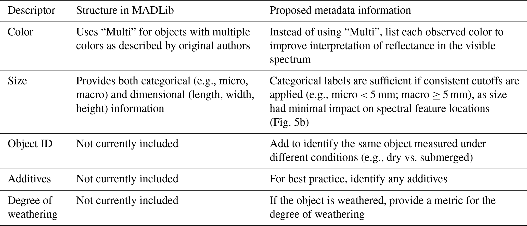
MADLib would benefit from more complete metadata and greater representation of common debris types to increase its utility, as missing or inconsistent metadata currently hinders algorithm development. For example, the reflectance spectrum of a plastic object (e.g., a dry cup) offers limited insight if essential metadata like polymer type, color, or experimental design are missing. Many published datasets included in MADLib exhibited this issue. To address this, we propose a comprehensive metadata structure (Table B1) for future marine debris reflectance studies. We sorted potential metadata into “required”, “best practice”, and “as needed” categories, acknowledging that some metadata maybe be difficult to obtain or unnecessary for future studies. Table B2 summarizes the proposed changes to existing parameters (color and size) and introduces three new parameters (object ID, additives, and degree of weathering).

Future additions to MADLib should prioritize providing data on debris types that are currently under-represented within the collection. For example, polymers such as PS, PE, and PPA along with colors like yellow, green, brown, and red have been recorded in marine debris surveys (Mutuku et al., 2024; Martí et al., 2020) but are poorly documented in MADLib (Figs. 5a, 7a). Furthermore, floating samples were rarely included in MADLib (Fig. 10a), yet they are the most detectable type of marine debris via remote sensing, warranting their characterization in future efforts. In addition, differences in the slopes of spectral features among samples of the same polymer type highlight the need for further investigation into the causes of such variability (Fig. 5c–d). Differences in manufacturing processes, the presence of additives, and variations in experimental design are all potential factors that could contribute to these discrepancies. Future work should examine the effects of additives and other manufacturing treatments within the same polymer type, as these may influence optical properties and, by extension, detection and classification accuracy.

While our initiative focused on reflectance, the most widely available optical parameter, future curation efforts that incorporate additional optical properties will expand the applicability of MADLib across a broader range of sensors, including active systems (Palombi and Raimondi, 2022; Goddijn-Murphy et al., 2024; Behrenfeld et al., 2023; de Fockert et al., 2024).

MADLib also paves the way for collaborations among remote sensing scientists, modelers, and marine policy experts. The current dataset may also support mapping debris movement and, when combined with physical transport models, can be used to forecast debris pathways to inform cleanup efforts and promote polluter accountability (Maximenko and Hafner, 2024). Lastly, we would like to emphasize the need for open-science and open-access approaches to move this effort forward.

5 Data availability

MADLib is available in open-access via https://doi.org/10.4121/059551d3-2383-4e20-af2d-011c9a59d3ac (Ohall et al., 2025). Two CSV files are included with the MADLib download: a metadata sheet and a data sheet. The samples can be linked across the two files using the dataset number and sample number columns.

6 Conclusions

MADLib represents a foundational step toward harmonizing spectral reflectance measurements for marine debris and is aligned with open-science policies. An important feature of the established MADLib collection is the traceable curation that allows ingestion of data from any permanent repository, dataset or reference library (e.g., Ocean Scan, PANGAEA, SeaBASS, SPECCHIO, USGS Spectral Library). We envision MADLib as a living resource where new datasets can be added to maximize interoperability and findability of the collection. We believe that prioritizing the measurements and metadata gaps discussed in future research will strengthen MADLib as a remote sensing community resource. With its currently available data, and future iterations, MADLib will further support algorithm development and help establish important specifications for debris detection to be implemented in future remote sensing technologies.

Appendix A

Figure A1 Mean reflectance spectra of four polymer types – HDPE, PP, PS, and PVC – submerged to depths between 5–715 mm.

Figure A2 Isolated reflectance spectra of floating samples from Fig. 10b and d.

Appendix B

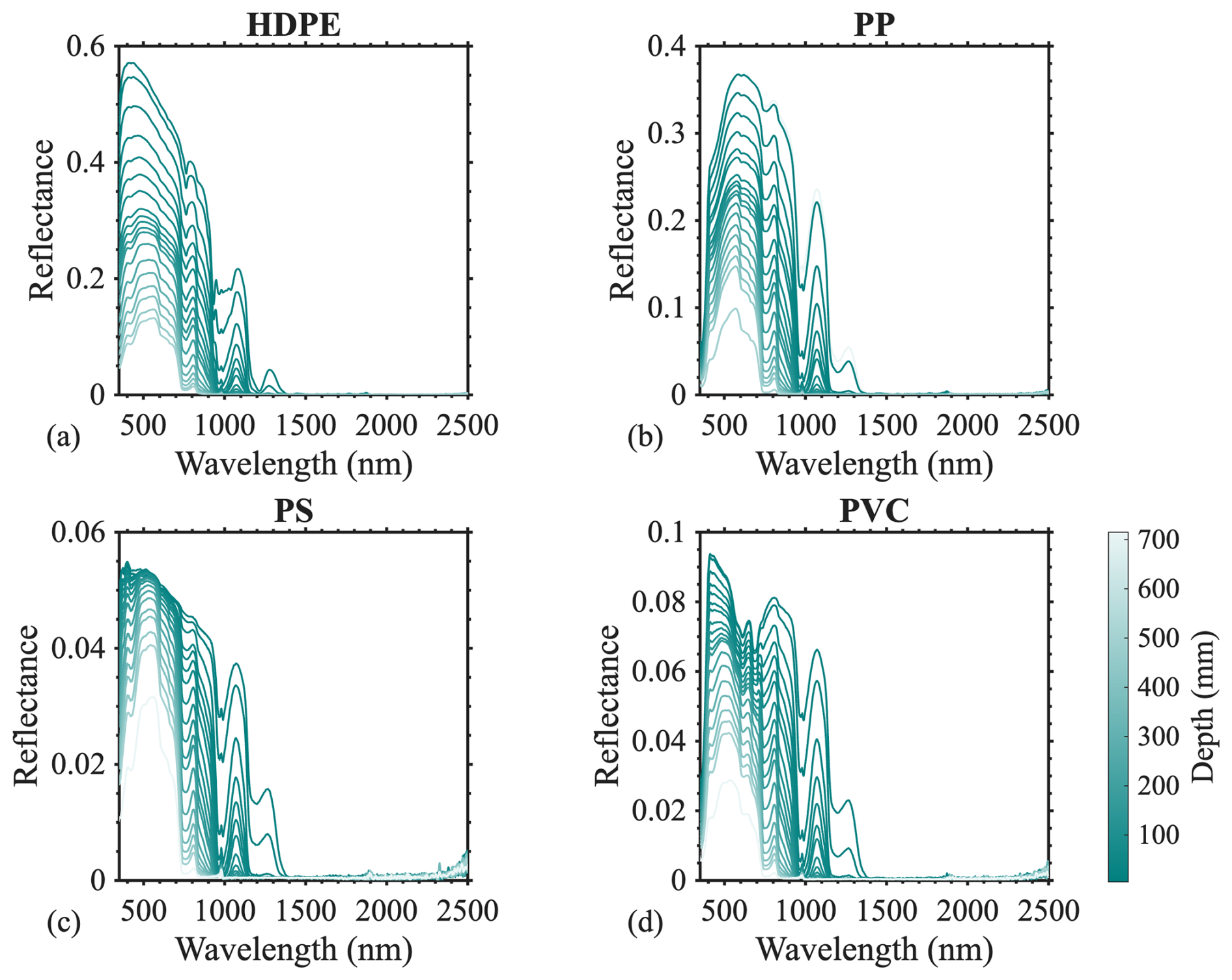
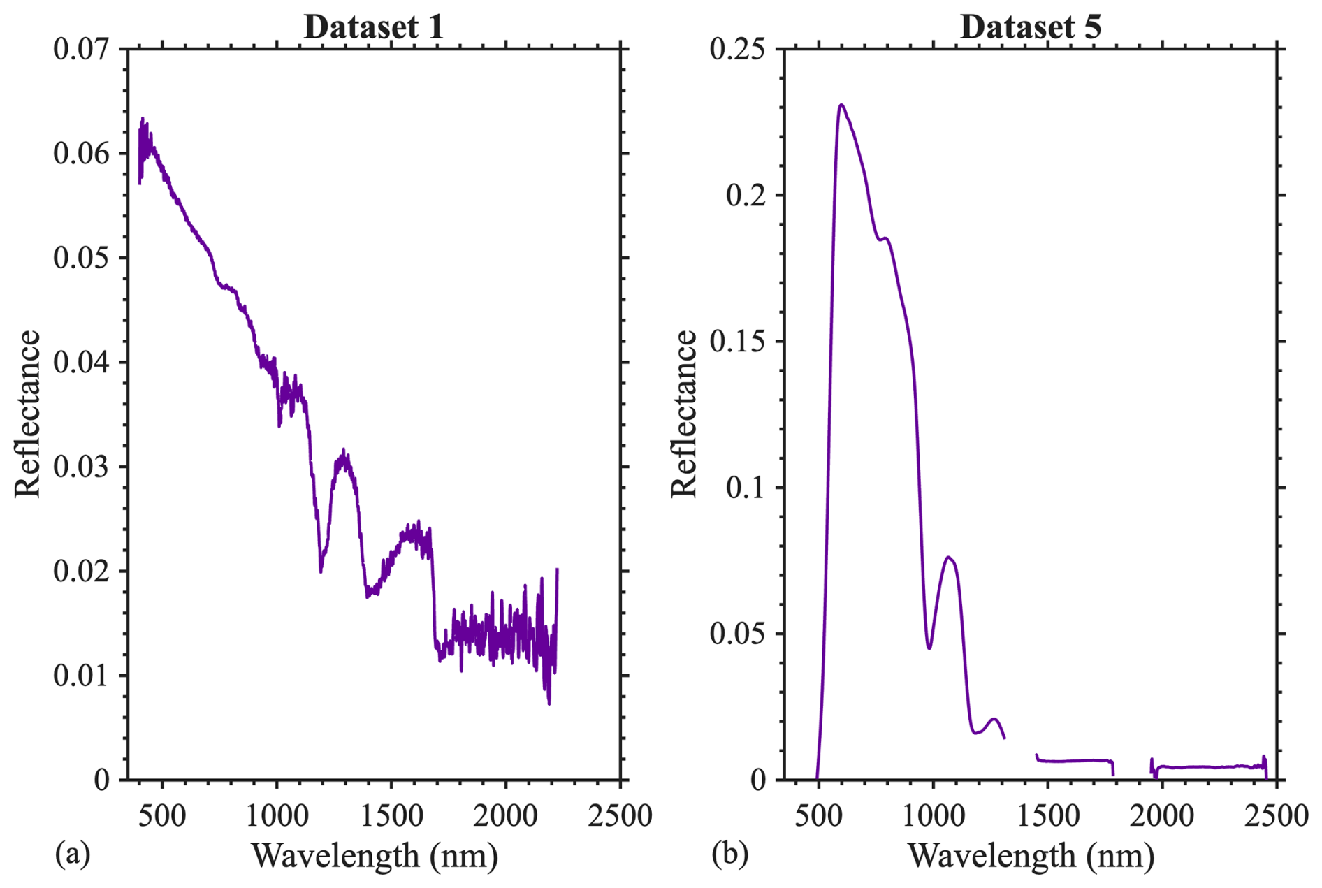
Table B1 Recommended metadata for future datasets, with required, best practice, and as needed metadata. See Table 2 for descriptions of metadata parameters.

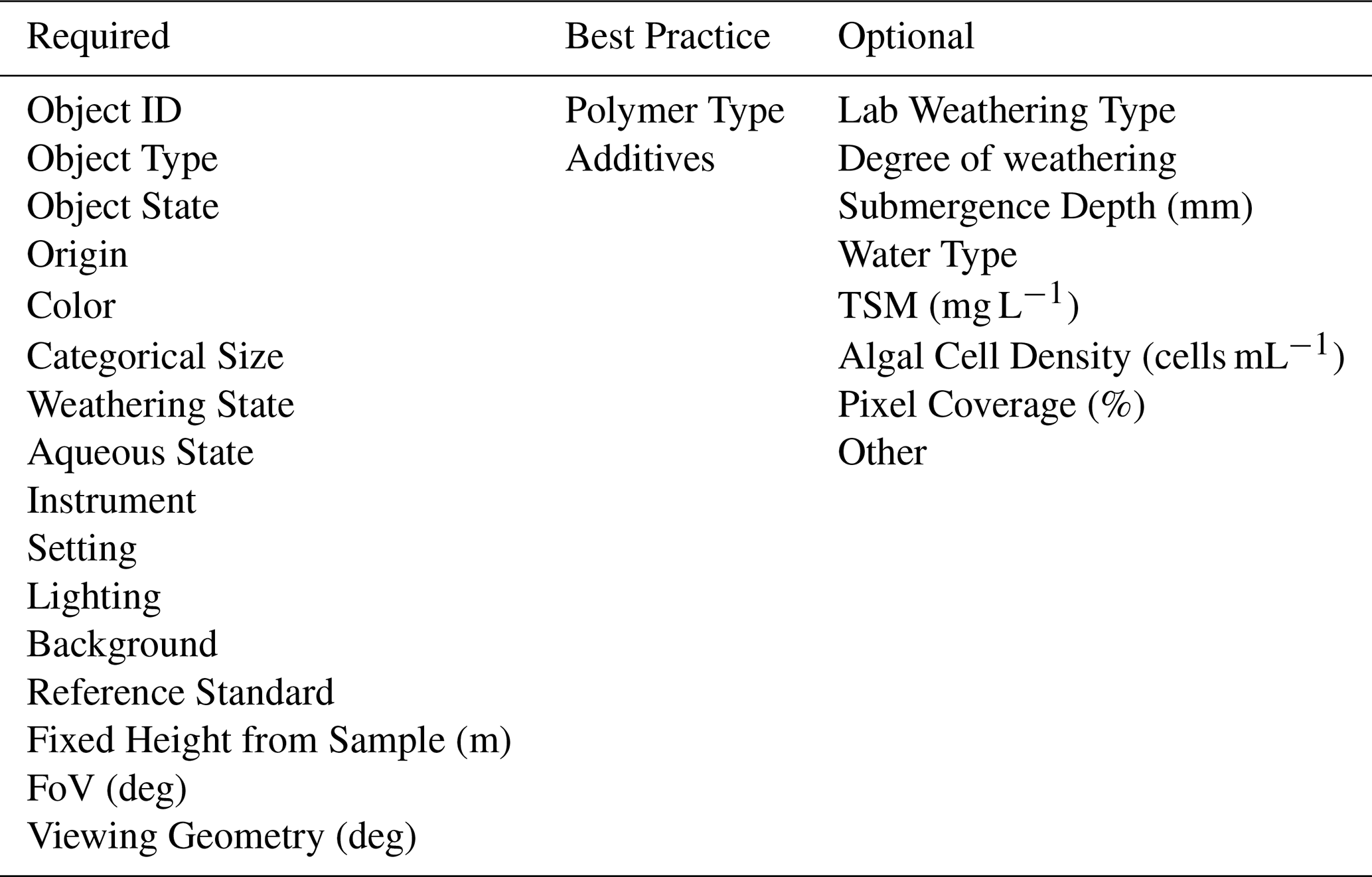
Table B2 Recommended improvements for future metadata collection of specific descriptors.