CropLayer: a 2 m resolution cropland map of China for 2020 from Mapbox and Google satellite imagery

Accurate and detailed cropland maps are essential for food security, yet existing products for China exhibit substantial discrepancies. This study presents CropLayer, a 2 m resolution cropland map of China for 2020, developed from Mapbox and Google satellite imagery. The framework comprises three key stages: (1) image quality assessment (IQA) using a ResNet model to compensate for missing acquisition metadata; (2) cropland extraction via an active learning strategy guided by a Mask2Former segmentation model and XGBoost-based semantic correctness evaluation; and (3) integration of Mapbox and Google results through an XGBoost model informed by four feature groups: Geography, IQA, Regional Property, and Consistency. A three-level validation scheme (pixel, block, and region) ensures robust and interpretable accuracy across spatial scales. CropLayer achieves a pixel-level accuracy of 88.73 %, a block-level semantic correctness of 96.5 %, and provincial-level consistency, with 30 out of 32 provinces showing area estimates within ±10 % of official statistics. In comparison, only 1–9 provinces meet this criterion across eight existing datasets. CropLayer provides a reliable, high-resolution baseline for agricultural structure analysis, yield estimation, and land use planning in China. The CropLayer dataset is available at https://doi.org/10.5281/zenodo.14726428 (Jiang et al., 2025).

1 Introduction

China, with its extensive agricultural resources and long-standing tradition of intensive farming, plays a pivotal role in global food production. Despite possessing less than 7 % of the world's cropland and only 5 % of utilizable freshwater resources, China produces nearly a quarter of the world's food, supporting more than 22 % of the global population (Kuang et al., 2022) (Zhang et al., 2022). This remarkable contribution highlights China's significance for both national and global food security, particularly in the face of increasing climate variability, natural disasters, and growing uncertainties in international food supply chains (Piao et al., 2010; Kang and Eltahir, 2018).

Accurate cropland maps are indispensable for agricultural monitoring, yield estimation, disaster loss assessment, and sustainable land management (Wu et al., 2023). High-resolution maps provide detailed spatial information essential for food security evaluation and policy making. Over the past two decades, cropland mapping has progressed considerably, with spatial resolutions advancing from coarse (1 km, 500 m) to medium (30 m, 10 m) (Cui et al., 2024a), and more recently approaching sub-meter scales (Li et al., 2023). While these improvements have enhanced the detection of cropland dynamics, challenges persist in capturing the diversity and fragmentation of smallholder farming systems, especially in China.

Several publicly available cropland datasets exist for China. Representative medium-resolution products include: (1) Dataset of China's annual cropland (CACD) (Tu et al., 2024), (2) the China land cover dataset (CLCD) (Yang and Huang, 2021), (3) Finer Resolution Observation and Monitoring of global land cover (FROM) (Gong et al., 2019), (4) Global land-cover product with Fine Classification System 2020 (FCS30) (Zhang et al., 2021), and (5) Globeland30-2020 (GL30) (Jun et al., 2014). Products based on 10 m Sentinel data include: (6) WorldCover from European Space Agency (ESA) (Zanaga et al., 2021) and (7) Land Cover v2 from the Environmental Systems Research Institute (ESRI) (Karra et al., 2021). Recently, high-resolution products have also emerged, such as (8) the national-scale land-cover map of China (SinoLC) derived from Google Earth imagery (Li et al., 2023).

Despite this progress, these datasets exhibit three recurring issues: (1) low consistency across products (Cui et al., 2024b); (2) inaccurate delineation of field boundaries, especially for smallholder plots (Qiu et al., 2024); and (3) extreme deviations in area estimation, for instance, our preliminary analysis indicates that in Guangdong Province, the reported cropland area in some datasets is up to 300 % of official statistics (Jiang et al., 2024). These problems largely stem from three factors: (1) insufficient spatial resolution of input imagery; (2) sampling strategies that lack representativeness (Zhang et al., 2020); and (3) overfitting caused by validation approaches that rely on single-dimensional accuracy metrics while neglecting multi-scale consistency.

Most existing cropland products are developed based on Landsat (Hansen and Loveland, 2012) and Sentinel (Bontemps et al., 2015; Qiu et al., 2022) imagery, with resolutions ranging from 10–30 m and relatively short revisit cycles. These data are valuable for capturing dynamic crop growth patterns, but they also face intrinsic challenges in cropland mapping. First, croplands are highly heterogeneous, with diverse crop types that are easily confused with non-cropland classes such as forest and grassland. Second, unlike crop phenology, cropland extent typically remains stable over multiple years, with relatively sharp and persistent boundaries and smoother textures, features that cannot be effectively captured by 10–30 m imagery (Liu et al., 2020). Particularly in southern China, where smallholder fields are often less than 0.1 ha, only meter-level imagery can adequately delineate cropland boundaries.

High-resolution (HR) remote sensing data offer a promising solution. Sub-meter imagery can capture detailed boundary and texture information that is essential for cropland mapping, especially in fragmented agricultural landscapes. Nevertheless, HR data also bring new challenges: longer revisit cycles, cloud contamination, and limited coverage, often requiring mosaicking from multiple satellite sources. Fortunately, freely available Google imagery (up to 0.3 m resolution) and cost-effective Mapbox imagery provide global coverage at meter-level resolution, and have shown strong potential in land cover mapping.

Despite their advantages, several challenges arise when using HR imagery for nationwide cropland mapping:

1. Lack of metadata and phenological information. Publicly accessible HR imagery often lacks metadata (e.g., acquisition dates, sensor types, image quality), which are crucial for crop monitoring.

2. High annotation cost for semantic segmentation. Unlike traditional sample-based classification, cropland mapping requires delineating continuous field boundaries in addition to labeling categories, making sample collection more expensive and less efficient. Random stratified sampling on geography space further increases redundancy and reduces annotation efficiency.

3. Difficulties in validation. Conventional pixel-level accuracy metrics are insufficient to detect overfitting or structural errors, which may lead to extreme regional biases. Large-scale visual inspection is also impractical given the data volume of nationwide HR imagery.

To address the challenges of large-scale cropland mapping, we designed a three-stage framework that integrates coverage assessment, efficient sample selection, and multi-modal validation.

First, we conducted coverage type assessment to ensure reliable input imagery. Using a ResNet-based classifier, each 2.4 m Google and Mapbox image tile was categorized into five types: Planting, Non-planting, Snow/Ice, Cloudy, and Nodata. This step provides metadata-like proxies (e.g., seasonality, contamination, or unusable regions) and enables subsequent results integration of imagery according to coverage types, rather than discarding any data, which may be partially useable.

Second, we implemented efficient sample selection through Active Learning (AL) in the feature space, which prioritizes the most informative samples and reduces annotation costs compared with random or stratified sampling (Settles, 2009). For semantic segmentation tasks, where object-level boundaries rather than point-wise labels must be annotated, this strategy substantially lowers labeling cost while ensuring sample diversity (Safonova et al., 2023). We evaluated widely used architectures, including PSPNet (Zhao et al., 2017), PIDNet (Xu et al., 2023), Segformer (Xie et al., 2021), and Mask2Former (Cheng et al., 2022). These were integrated into this stage to guide the choice of the most effective segmentation model within the AL loop.

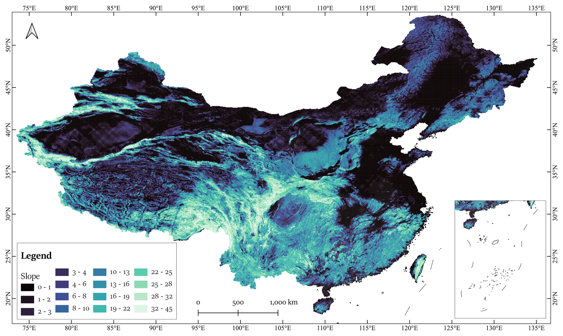
Figure 1 Slope distribution in the Study Area of China.

Third, we established a multi-modal validation scheme to guarantee both local accuracy and regional consistency. This scheme comprises (1) pixel-level accuracy assessment, (2) image block-level (0.05° × 0.05°) semantic correctness assessment, which evaluates whether the mapped cropland distribution matches the expected semantics of agricultural landscapes, and (3) region-level area comparison with statistical records. Together, these metrics mitigate risks of overfitting and ensure that errors are detectable across multiple spatial scales.

Using this framework, we generated the nationwide CropLayer dataset from 2.4 m (zoom level 16) Google and Mapbox imagery, integrating coverage type assessment, cropland extraction, and result synthesis. CropLayer was evaluated against 8 publicly available cropland products in terms of accuracy, area estimates, and consistency, with further analyses on regional discrepancies and implications for agricultural monitoring and resource management.

2 Study area and data

2.1 Study area

The study area encompasses the entirety of China, located in the eastern part of the Eurasian continent, with a total land area of approximately 9.6 million km². Cropland in China covers about 127.9 million ha, ranking it as the third-largest country globally in terms of cropland area. The country's topography is highly varied, with mountains, plateaus, and hills accounting for approximately 67 % of the land area, while basins and plains make up the remaining 33 % (Liu et al., 2024). This complex terrain, combined with diverse climatic conditions, results in substantial regional variability in agricultural practices and cropland types (Fig. 1).

China's primary cropland types include dry land, paddy fields, and irrigated land (Zhang et al., 2024). Flat terrains in basins and plains, such as the Northeast Plain, North China Plain, the middle and lower Yangtze River Plains, and the Chengdu Basin, are well-suited for large-scale mechanized farming due to concentrated land resources. Conversely, mountainous, plateau, and hilly regions, particularly in Southwest China, feature rugged terrain and fragmented arable land, posing significant challenges to large-scale agricultural development (Li et al., 2022).

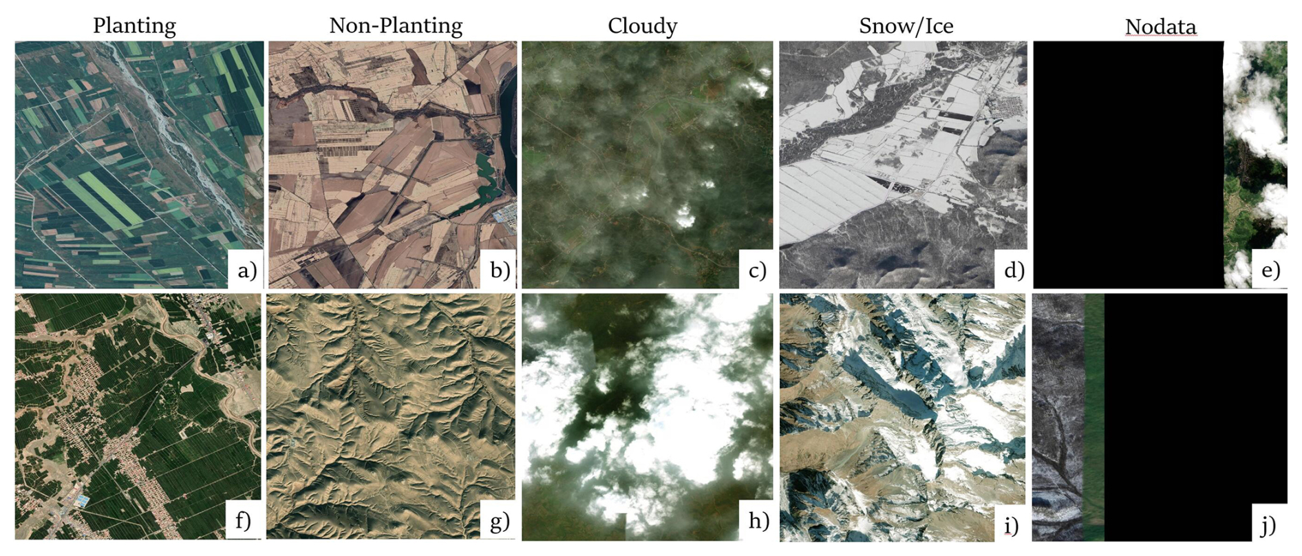
Figure 2 Examples of 5 Coverage type. The HR remote-sensing images in the figure are from ©Mapbox 2023 and ©Google Maps 2023.

2.2 Data

2.2.1 High Resolution Remote Sensing Imagery and Data Structure

The CropLayer dataset was generated using HR satellite imagery from Mapbox and Google. These imagery datasets are continuously updated from various sources, including commercial providers, NASA, and USGS. According to the Google (http://mts0.googleapis.com, last access: 26 November 2025) and Mapbox (https://api.mapbox.com/v4/mapbox.satellite, last access: 26 November 2025) Satellite services, global HR satellite imagery is provided as RGB color patches with a resolution of 256 pixel × 256 pixel and is accessible via a Web Map Service (WMS) API. The imagery used in this study was accessed between August 2022 and December 2023.

Although the datasets lack key metadata, such as sensor type, viewing angle, and atmospheric conditions, they undergo extensive radiometric and geometric corrections before being made publicly available. These corrections ensure data reliability and suitability for various applications, including cropland mapping.

In this study, the HR imagery was organized into image blocks measuring 0.05° × 0.05° in WGS 1984 geographic coordinates, with each block comprising mosaicked image patches. A total of 389 777 image blocks were generated, covering the entire extent of China for both datasets. The imagery was utilized at level-16, corresponding to a spatial resolution of approximately 2.4 m per pixel, which is sufficient for capturing the geometry and structure of cropland.

2.2.2 DEM Data

Given the strong correlation between cropland distribution and topographic features, this study utilized Digital Elevation Models (DEM) to improve cropland mapping accuracy. Due to the lack of high-resolution DEM data, it was not included in the initial cropland extraction phase. Instead, 30 m resolution DEM data from the Shuttle Radar Topography Mission (SRTM) was incorporated during the post-processing stage. Key topographic features including slope, ruggedness, and roughness were derived from the DEM using the gdaldem tool (https://gdal.org/en/latest/programs/gdaldem.html, last access: 26 November 2025).

2.2.3 Samples 1: Coverage type classification

All image blocks were categorized into five distinct coverage types (Fig. 2): Planting, Non-Planting, Cloudy, Snow/Ice, and Nodata, represented by the color codes green, yellow, white, light grey, and black, respectively. Due to the relative scarcity of blocks classified as Cloudy, Snow/Ice, and Nodata, an AL strategy was adopted for sampling, enabling the selection of blocks with more distinct features. This approach improved class discriminability compared to systematic sampling methods.

Table 1 Definition of image coverage type.

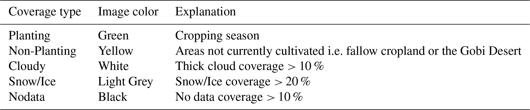
Definitions for each coverage type are outlined in Table 1. From the datasets, a total of 8084 image blocks were curated from various regions of China, ensuring comprehensive coverage. These blocks were further divided into 6465 training samples and 1619 validation samples to provide a robust and diverse dataset for model training and evaluation.

2.2.4 Samples 2: Cropland extraction

Cropland samples were manually labelled using HR imagery in shapefile format via QGIS software. These samples were not collected in a single phase but were gradually acquired through an AL strategy (Mittal et al., 2023). Initially, the model was trained on a preliminary set of samples. The predicted results were then visually inspected, and additional samples were collected from areas with the most significant errors to improve model accuracy.

Table 2 Typical representatives of various types of cropland and non-cropland. The HR remote-sensing images in the figure are from © Mapbox 2023 and © Google Maps 2023.

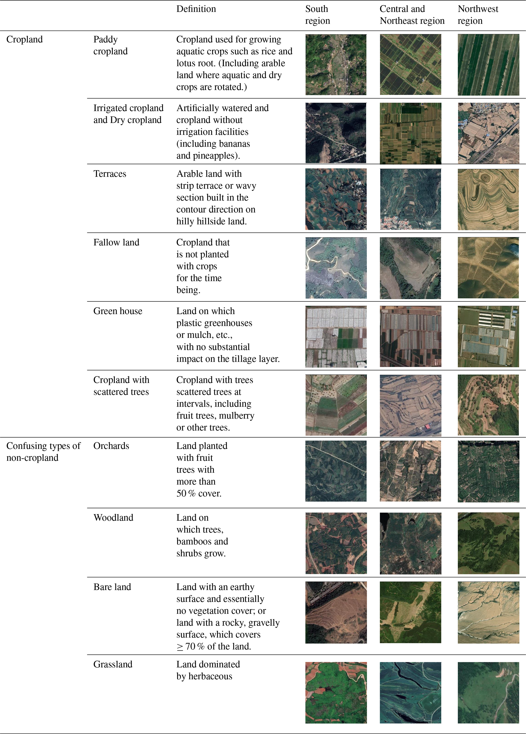
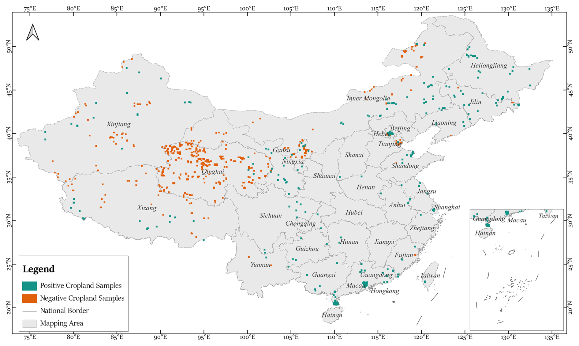
Figure 3 Distribution of positive and negative cropland samples.

The spatial distribution of the labelled samples is illustrated in Fig. 3, while examples of the labeled data are provided in Table 2.

To enhance model robustness, the cropland samples were designed to encompass diverse cropping practices and crop types. The dataset consists of 157 395 polygons, most of them representing an individual cropland, distributed across 366 image blocks (0.05° × 0.05° each), collectively referred to as positive cropland samples (Fig. 3).

In addition to these positive samples, the dataset includes 761 negative cropland samples blocks devoid of cropland polygons. These negative samples are particularly important as they often feature areas resembling cropland but are not actual cropland. Their inclusion strengthens the model's ability to differentiate between cropland and non-cropland regions, thereby improving classification accuracy.

2.2.5 Samples 3: Semantic correctness and results integration

A data-driven approach is adopted for both semantic correctness and results integration during the cropland extraction process. Systematic grid sampling at intervals of 0.5° longitude and latitude is applied, generating a total of 3891 image blocks. The process involves two key steps:

1. Semantic correctness. Systematic sampling was first applied to select 3891 points, which were then independently interpreted for Google and Mapbox imagery, producing two separate sets of results for the same locations, yielding 7782 samples categorized into four groups:

   • a.

     True Positive (TP): Correctly identified croplands.

   • b.

     False Positive (FP): Non-cropland areas mistakenly identified as cropland.

   • c.

     Noise: Very small extraction errors.

   • d.

     Artifacts: Misclassified areas due to imagery inconsistencies or processing errors.

2. Results Integration. The same set of 3891 blocks was classified into four integration categories:

   • a.

     Neither Source: Blocks where neither dataset identifies cropland.

   • b.

     Only Mapbox: Blocks with cropland identified exclusively by Mapbox.

   • c.

     Only Google: Blocks with cropland identified exclusively by Google.

   • d.

     Merging Both: Blocks where cropland is identified in both datasets, integrated for improved accuracy.

To ensure comprehensive evaluation and reliable result integration, a systematic sampling and categorization approach was adopted. For model classification, the total sample set was stratified and randomly split, allocating 80 % for training and 20 % for testing. This method enhanced model accuracy and improved the reliability of the final cropland dataset.

2.2.6 Cropland definition and statistical area

Provincial-level cropland statistics for China were obtained from the Third National Land Survey (TNLS), a nationwide initiative that conducted a detailed assessment and verification of land resources, including the extent and distribution of cultivated land. The survey employed professional investigators and a hierarchical inspection system to ensure data accuracy and reliability, making the TNLS statistics a robust reference for comparative analysis and validation.

In this study, the definition of cropland used in CropLayer strictly follows the criteria established in the TNLS. It includes cultivated land used for growing crops such as paddy fields, irrigated land (including greenhouses used for planting), and dry land, as well as land used for temporary crops including medicinal plants, grass, flowers, and trees. It also encompasses newly developed or reclaimed land, fallow land, and areas where crop cultivation predominates, even if interspersed with occasional fruit trees or other vegetation. However, it explicitly excludes orchards, which are classified separately in the TNLS as Plantation land. This definition ensures conceptual consistency between CropLayer and national statistical data.

This study focuses on 32 provincial units in China with cropland areas exceeding 100 km², excluding Hong Kong and Macau. Cropland statistics for Taiwan are not covered by the TNLS and were obtained from alternative sources (https://agrstat.moa.gov.tw/sdweb/public/indicator/Indicator.aspx, last access: 26 November 2025). Notably, the definition of cropland in Taiwan differs from the TNLS standard, as it includes orchards and other perennial crop lands.

2.2.7 Existing cropland data

To evaluate the performance of CropLayer, we employed eight existing cropland or land-cover (LC) datasets:

• 1.

  Dataset of China's annual cropland (CACD) from Tsinghua University (Tu et al., 2024),

• 2.

  China land cover dataset (CLCD) from Wuhan University (Yang and Huang, 2021),

• 3.

  WorldCover from European Space Agency (ESA) (Zanaga et al., 2021),

• 4.

  Land cover v2 from the Environmental Systems Research Institute (ESRI) (Karra et al., 2021),

• 5.

  Finer Resolution Observation and Monitoring (FROM) of global land cover from Tsinghua University (Gong et al., 2019),

• 6.

  Global land-cover product with Fine Classification System (FCS30) 2020 from Aerospace Information Innovation Institute, Chinese Academy of Sciences (Zhang et al., 2021),

• 7.

  Globeland30-2020 (GL30) from National Geomatics Center of China (Jun et al., 2014),

• 8.

  National-scale land-cover map of China (SinoLC) from China university of geosciences (Li et al., 2023).

Table 3 Summary of 8 existing cropland/land cover data.

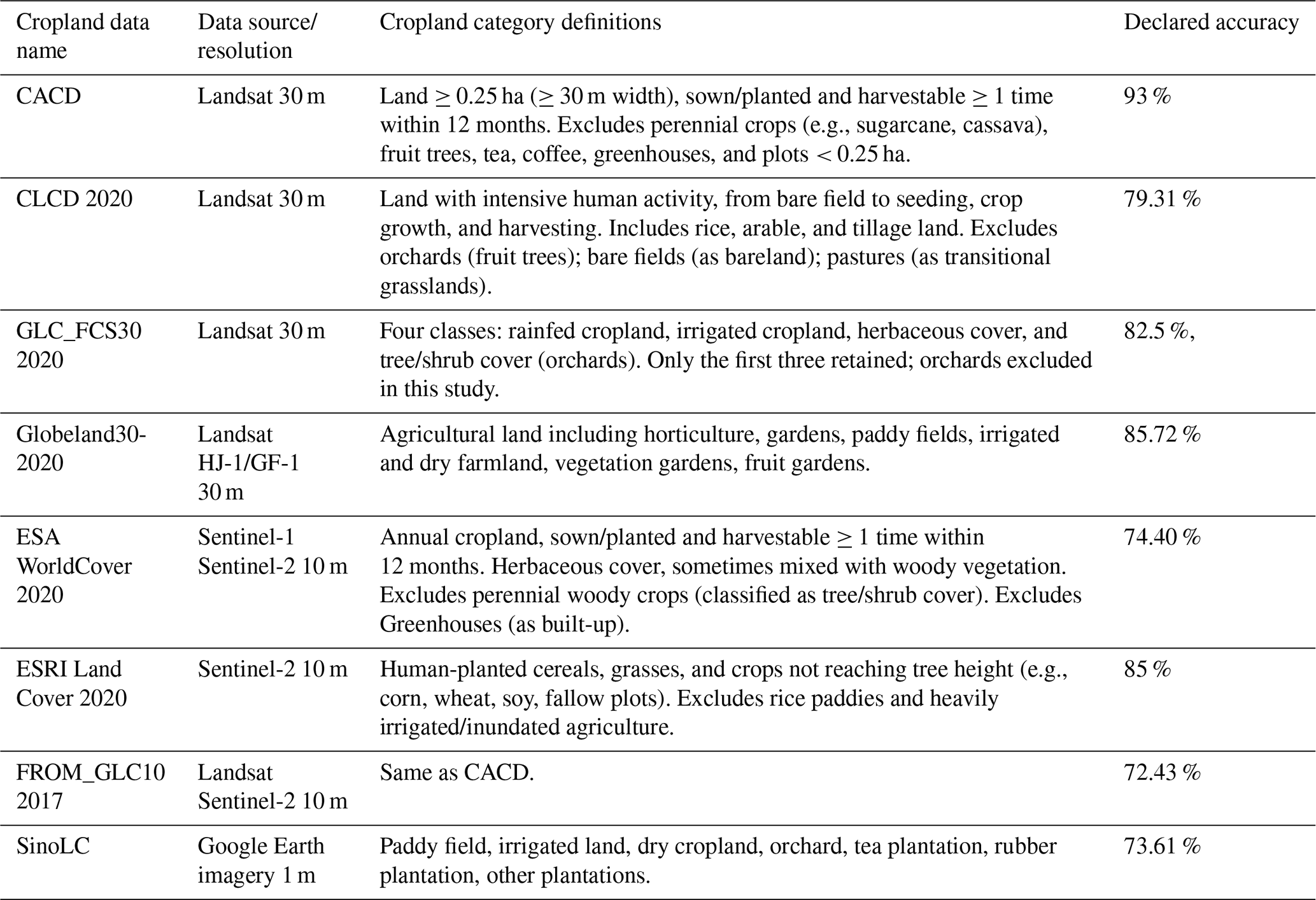
These datasets are primarily derived from Sentinel or Landsat imagery, except SinoLC, which is based on Google Earth imagery consistent with this study. They were generated using human-interpreted samples combined with machine learning methods. A summary of their characteristics is provided in Table 3. All datasets correspond to the year 2020, except FROM (2017), though provincial-level cropland differences remain comparable. Reported overall accuracies range from 72 % to 93 %.

Figure 4 Cropland category definitions in CropLayer versus 8 existing cropland datasets.

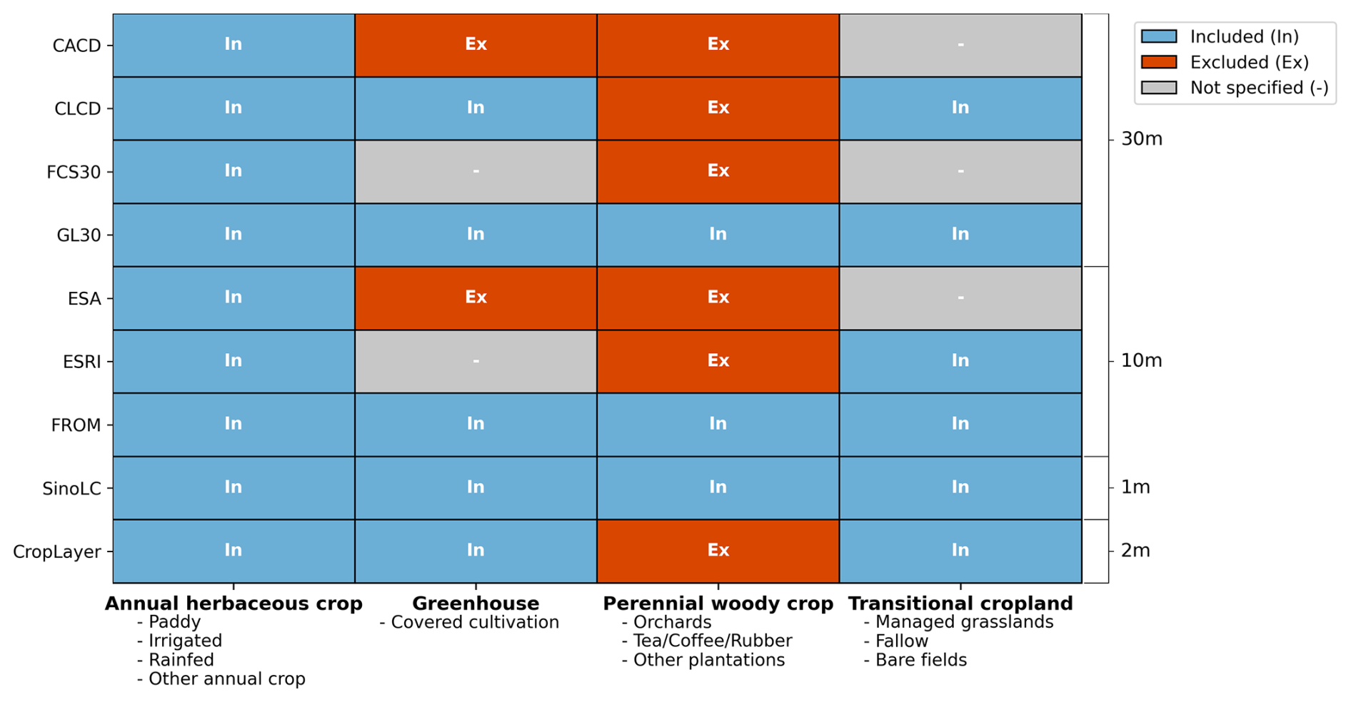
Table 3 also highlights differences in cropland definitions, particularly regarding greenhouses, perennial woody crops, and transitional cropland. To facilitate comparison, we developed a unified superset classification with four groups (Fig. 4):

• Annual herbaceous crops form the core of cropland, consistently included across datasets, covering staple systems such as paddy fields, irrigated, and rainfed croplands.

• Greenhouse crops show inconsistent treatment: CACD and ESA exclude them, ESRI and FCS30 provide no explicit statement, and the remaining datasets generally include them, though their national extent is relatively small.

• Perennial woody crops (e.g., orchards, tea, and rubber) differ substantially from annuals in phenology and management. Most datasets map them separately as distinct land-cover classes, with only FROM, GL30, and SinoLC including them within cropland.

• Transitional cropland (e.g., fallow, managed grassland, or temporarily bare fields) is the least clearly defined. These heterogeneous lands lack stable features, and while all datasets allow some inclusion, CACD, ESA, and FCS30 are less explicit in their definitions.

  This heterogeneity in category definitions contributes to inconsistencies in cropland area estimates across products.

Figure 5 Flowchart of cropland mapping.

3 Methods

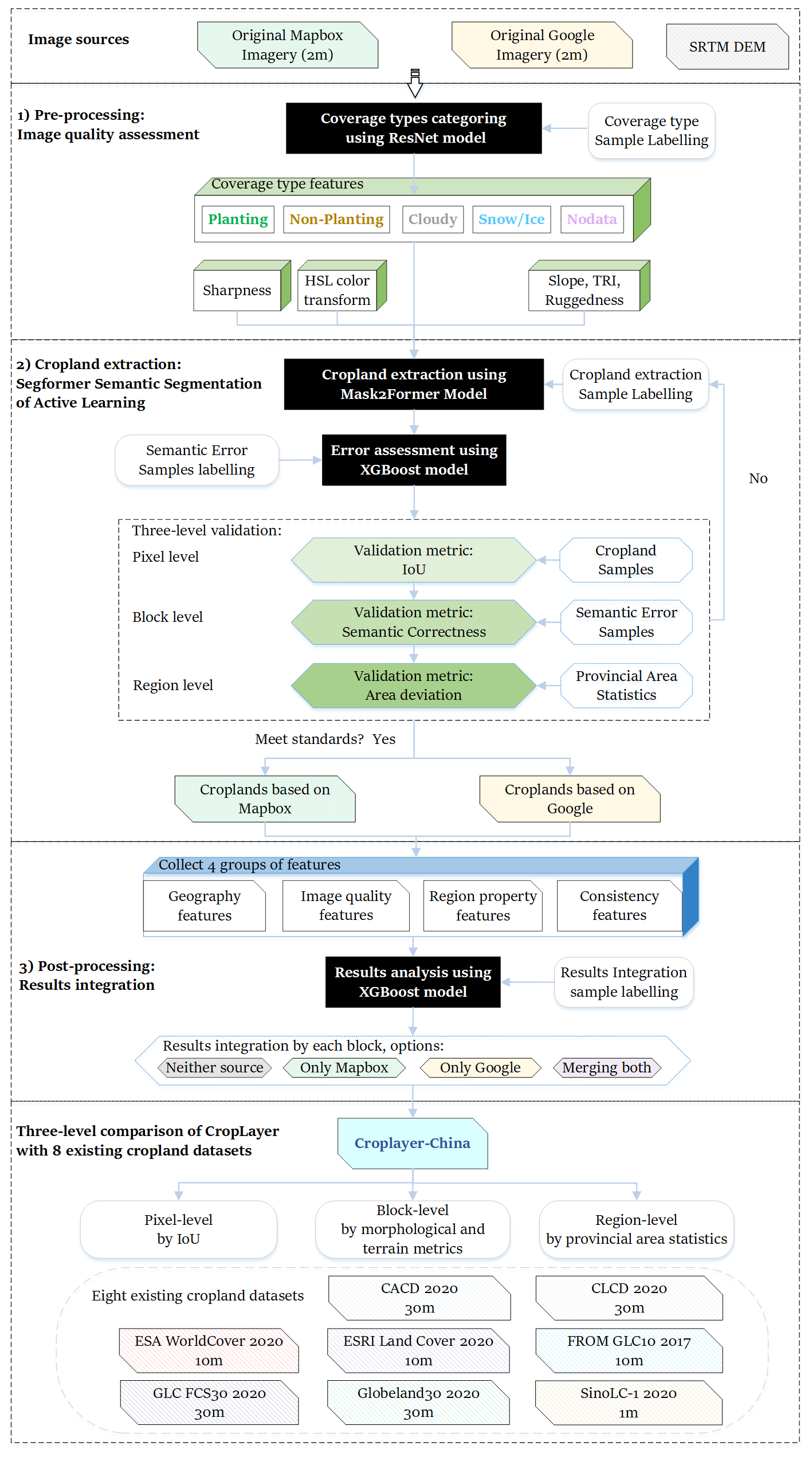
This study proposes a framework for cropland mapping using 2 m high-resolution imagery from Mapbox and Google. The framework consists of three key stages (Fig. 5):

• 1.

  Pre-processing: The national imagery is divided into 0.05° × 0.05° blocks to facilitate efficient parallel processing (Yang et al., 2019). Image Quality Assessment (IQA) is performed on both imagery sources using ResNet models (He et al., 2016), compensating for the lack of acquisition metadata.

• 2.

  Cropland Extraction: An AL-based model for cropland identification is developed, utilizing Mask2Former for semantic segmentation and XGBoost (Chen and Guestrin, 2016) for semantic correctness.

• 3.

  Post-processing: The two datasets are integrated through a merging strategy driven by XGBoost, using four feature groups: Geography, IQA, Region Property, and Consistency. The resulting national cropland map is referred to as CropLayer.

The accuracy and reliability of CropLayer were further evaluated by comparing it with eight publicly available cropland datasets and statistical area information.

3.1 Pre-processing: image quality assessment

The identification of croplands using satellite imagery from Mapbox and Google is often hindered by low-quality images, including those affected by no-data regions, cloud cover (thick and thin), snow/ice, and land fallow periods. To address these challenges, an image quality assessment (IQA) method was developed to guide the selection of optimal datasets.

IQA replicates human perception of image quality and serves two key purposes: filtering out poor-quality images to improve downstream tasks such as alignment, fusion, and recognition, and evaluating the performance of post-processing algorithms (Zhu et al., 2020). IQA methods are broadly classified into with-reference and no-reference approaches (Gao et al., 2024). In this study, both were utilized: with-reference IQA for classifying easily identifiable features and no-reference IQA for detecting thin clouds through specialized feature calculations. The IQA outputs were integrated during post-processing to enhance cropland identification results.

• 1.

  Coverage Type Classification

  To classify image coverage types, we trained a ResNet-based image classification model using the samples described in Sect. 2.2.3. ResNet's deep residual architecture enhances feature extraction by addressing the vanishing gradient problem with skip connections, enabling the network to capture multilevel abstract features. This capability allows ResNet to excel in identifying complex image attributes such as color, texture, shape, and spatial context, thereby improving classification accuracy. Fine-tuning the pre-trained ResNet model on the dataset further enhances generalization and efficiency in coverage type classification.

• 2.

  Thin cloud features calculation

  Thin clouds pose a unique challenge, as they are difficult to detect through standard image classification methods. To address this, two features were calculated: the Gradient (Eq. 1) represents the sharpness of land cover boundaries, serving as an indicator of image clarity. The HSL (Hue, Saturation, and Lightness) captures color and saturation properties, aiding in the detection of subtle cloud contamination. These features collectively contribute to assessing the impact of thin clouds on image quality, enabling more accurate cropland identification during post-processing.

  $$\begin{array}{}\text{(1)}& \text{Gradient}=\text{Sobel}\left(\mathrm{RGB}\right)\end{array}$$

Here, the Sobel operator is applied to the RGB bands to measure edge intensity, reflecting image clarity. These features collectively support the identification of subtle thin-cloud contamination and improve downstream cropland extraction accuracy.

3.2 Cropland mapping: semantic segmentation of active learning

3.2.1 Active learning strategy

The AL workflow begins with an initial set of labeled image blocks used to train a Mask2Former segmentation model. The model then predicts cropland distributions in unlabeled regions. These predictions are manually reviewed, and blocks with substantial commission (false positives) or omission (false negatives) errors are added to the labeled pool for subsequent iterations. The process repeats until a convergence criterion is reached.

A key difficulty in AL is determining when to stop iterating. Early in the process, overestimation and underestimation errors are easily identified by inspection, but as the model improves, errors become subtler and less visually discernible. To address this, a three-level validation scheme was introduced to provide an objective basis for iteration control.

The validation assesses cropland extraction quality from pixel, block, and regional perspectives. It not only monitors model performance during AL but also defines the termination condition for training, ensuring that the model stops when no significant artifacts or omission errors are detected across regions. This multi-scale validation enhances both efficiency and reliability, preventing overfitting while maintaining high segmentation accuracy across diverse landscapes.

3.2.2 Mask2Former model

Mask2Former is a universal image segmentation framework capable of handling semantic, instance, and panoptic segmentation tasks through a Transformer-based decoder (Cheng et al., 2022). Unlike traditional Transformer decoders, it introduces a masked attention mechanism that restricts cross-attention operations to the foreground regions defined by predicted masks. This approach accelerates convergence and improves performance by focusing attention on local areas rather than the entire image, making it particularly effective for segmenting small objects. The model incorporates multi-scale, high-resolution feature inputs, allowing it to handle objects and regions of various sizes while iteratively refining mask predictions through multiple layers.

To enhance efficiency, Mask2Former optimizes the Transformer decoder by adjusting the order of self-attention and cross-attention for more effective feature learning. It also uses learnable query features, which provide more expressive initial queries without relying on random initialization. Additionally, the model reduces memory consumption by computing mask loss through random sampling, lowering memory usage by threefold while maintaining segmentation performance. These improvements enable Mask2Former to achieve high segmentation accuracy while significantly increasing training efficiency and reducing computational demands.

3.2.3 Three-level validation scheme

During the AL process, each iteration was conducted on at least one provincial unit. The provincial unit was selected because the available TNLS cropland area statistics are organized at the provincial level, providing a consistent reference for regional-level evaluation. After each iteration, a three-level validation scheme was applied to assess the mapping quality at different spatial scales:

1. Pixel-level

   At the pixel-level, accuracy was evaluated using the Intersection over Union (IoU) metric (Eq. 2):

   $$\begin{array}{}\text{(2)}& \text{IoU}={\displaystyle \frac{\text{TP}}{\text{TP}+\text{FP}\text{+ FN}}}\end{array}$$

   where TP (true positives) denote correctly identified pixels, FP (false positives) denote pixels incorrectly labeled as cropland, and FN (false negatives) denote missed cropland pixels. IoU provides a direct measure of pixel-wise agreement between predictions and reference samples.

2. Block-level

   At the block-level (0.05° × 0.05°), we quantified Region Properties (Burt et al., 1981) to characterize the geometric and topological structure of cropland distribution (Maryada et al., 2025; Bhosale et al., 2023). Specifically:

   Solidity: representing the compactness of cropland patches, was calculated as (Eq. 3):

   $$\begin{array}{}\text{(3)}& \text{Solidity}={\displaystyle \frac{\text{Area}}{\text{Area}\left(\text{Convex\hspace{0.17em}\hspace{0.17em}Hull}\right)}}\end{array}$$

   where Area is the pixel count in the cropland region, and Area(Convex  Hull) is the pixel count within its convex hull. Higher solidity indicates fewer irregularities in shape.

   Euler number: a topological metric defined as (Eq. 4):

   $$\begin{array}{}\text{(4)}& \text{EulerNumber}=C-H\end{array}$$

   where C represents the number of connected components (objects), and H is the number of holes within those components. A higher Euler number signifies fewer holes and better segmentation quality.

3. Provincial-level

   At the provincial scale, cropland area was aggregated and compared with official statistical records to ensure consistency with large-scale agricultural distributions.

Finally, incorporating multimodal-sources validation helps to reduce potential overfitting, which is more commonly observed in single-source validation, thereby providing a more robust assessment.

Table 4 Results refining options and explanations

Table 5 Evaluation features for each block.

3.2.4 Active Learning Stopping Criteria

To ensure both efficiency and reliability, quantitative stopping criteria were defined for each validation level. The iterative sampling-training-validation loop was terminated once all thresholds were met, indicating convergence in both classification accuracy and semantic consistency:

• Pixel-level criterion: IoU must reach at least 85 % within the targeted province. Lower values indicate ambiguous samples or insufficient separability, prompting additional sample refinement

• Block-level criterion: The semantic correctness, defined as the proportion of blocks with consistent cropland patterns and boundary integrity, must exceed 85 %, ensuring spatial structural coherence.

• Provincial-level criterion: The extracted cropland area from either imagery dataset must achieve at least 80 % agreement with official statistics. For provinces with persistent cloud contamination or limited high-quality imagery, the AL process is allowed to terminate after three supplementary sample labelling even if the threshold is not met.

Once these three conditions are satisfied (or the exception condition applies), the iteration for that provincial unit is concluded. This multi-level validation and stopping mechanism ensures stable, interpretable, and scale-consistent performance of the final CropLayer dataset.

3.3 Post-processing: cropland results integration

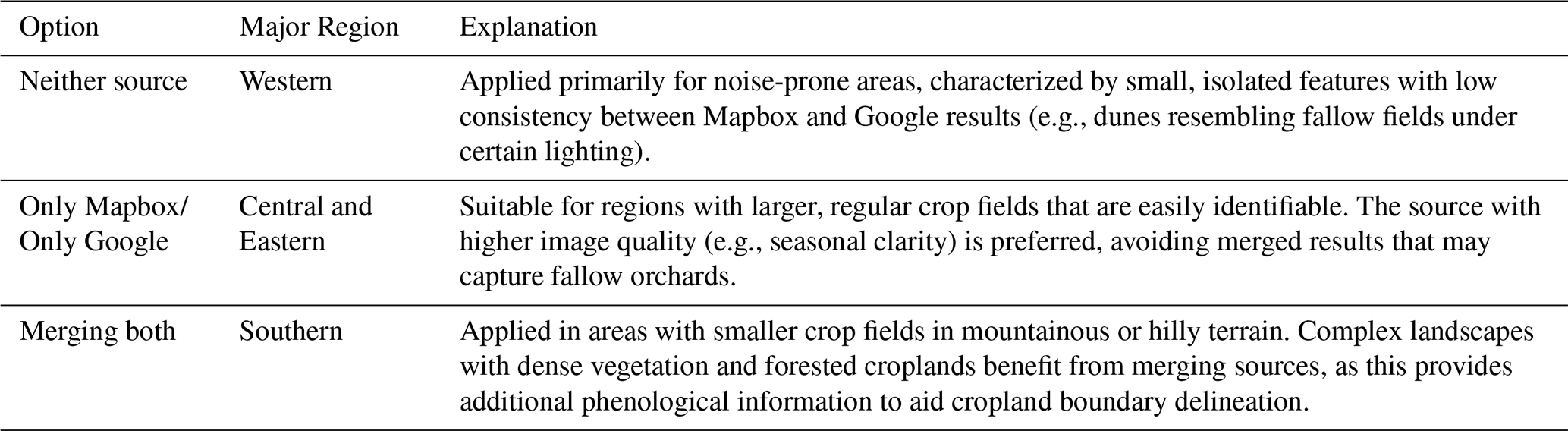
Using imagery from Mapbox and Google, two distinct cropland identification results were generated for each block across the study area. To create a final, higher-quality cropland map, an integration strategy was developed to combine the strengths of both datasets. Each block was assigned one of four integration options: Neither Source, Only Mapbox, Only Google, or Merging both, as detailed in Table 4.

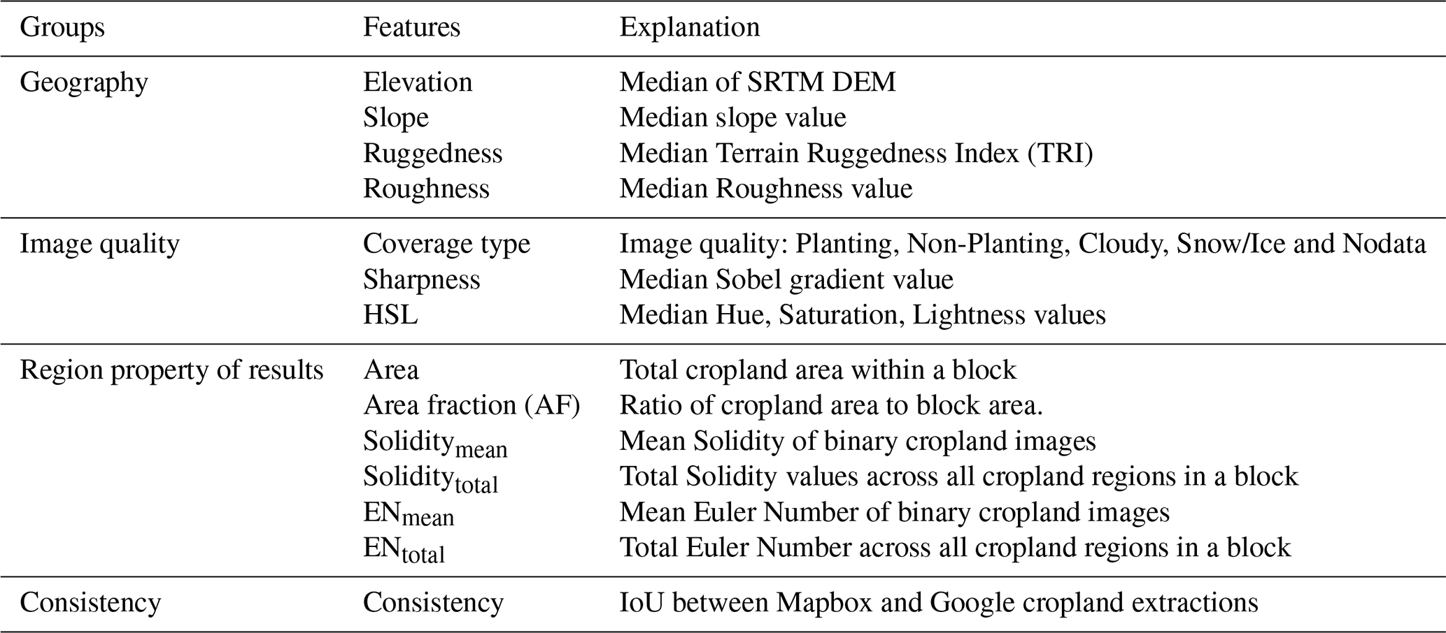
Four feature groups (Geography, Image Quality, Region Property, and Consistency) were extracted and used to train an XGBoost model that predicts the optimal integration strategy for each block. A total of 16 features such as area fraction (AF), Solidity, Euler Number, and IoU between the two sources were used to guide decision-making (Table 5) .

To clarify the contribution of each feature group in the XGBoost classification framework, we conducted a permutation importance analysis. This analysis was applied separately to the Semantic Correctness and Results Integration models.

The Semantic Correctness model used 16 features, including geographic, regional, and topographic attributes. The Results Integration model incorporated 30 features: 12 pairs from Mapbox and Google imagery, together with 4 shared topographic variables (slope, ruggedness, elevation, and roughness), and 2 prediction results of Semantic Correctness. Feature importance was derived from the mean decrease in model performance when each feature was randomly permuted.

3.4 Assessment metrics for three-level comparison of CropLayer with eight existing cropland datasets

After completing dataset integration, the final CropLayer product was evaluated by a three-level comparison against eight existing cropland datasets. This parallels the validation framework but focuses on comparative evaluation rather than process control.

All datasets were resampled to a 2 m resolution to ensure spatial consistency. The comparison was conducted at the pixel, block, and provincial levels, reflecting spatial agreement, structural characteristics, and large-scale reliability, respectively.

• 1.

  Pixel-level

  Pixel-wise agreement was quantified using IoU, indicating the extent of spatial overlap between CropLayer and each reference dataset.

• 2.

  Block-level

  At the block level, area fraction (AF) and edge density (ED) were computed as:

  $$\begin{array}{}\text{(5)}& \text{ED}={\displaystyle \frac{N}{N_{\mathrm{t}}}}\end{array}$$

  Where N is the number of cropland or boundary pixels; N_t the total number of pixels per block.

  The relative deviation from CropLayer was calculated as (Eq. 6):

  $$\begin{array}{}\text{(6)}& \text{Div}={\displaystyle \frac{T-C}{C}}\end{array}$$

  where T and C are the metric values for the target and CropLayer datasets, respectively.

  These deviation measures reveal overestimation and underestimation patterns and, combined with terrain attributes (e.g., slope median), help interpret topographic influences on discrepancies.

• 3.

  Provincial-level

  At the provincial level, cropland area was aggregated and compared with both reference datasets and official statistics. Provincial units with deviations within ± 10 % of the statistical cropland area were considered consistent, reflecting large-scale reliability.

4 Result

4.1 Image quality assessment

The Coverage Types classification model based on ResNet achieved a top-1 accuracy of 95.6 %. Figure 5 illustrates that high-quality categories (Planting and Non-Planting) account for similar proportions in Mapbox (82.8 %) and Google (82.1 %) blocks, though Mapbox contains more Planting (50.7 % vs. 41.3 %) and fewer Non-Planting (32.2 % vs. 40.8 %).

Lower-quality categories (Cloudy, Snow/Ice, Nodata) are nearly equivalent between the two datasets (17.2 % vs. 17.9 %). Among them, Cloudy imagery is more prevalent in Mapbox (8.5 % vs. 1.9 %), while Google has higher proportions of Snow/Ice (13.4 % vs. 8.3 %) and Nodata (2.6 % vs. 0.4 %).

Figure 6 Statistics of Coverage Types for Original Mapbox and Google Imagery.

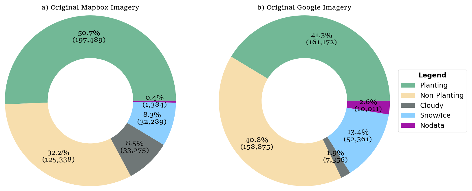
Spatially, Mapbox quality is poorer in southern China, and Google shows more Snow/Ice and Nodata in the northeast and west (Fig. 6). Hypothetically replacing low-quality blocks with high-quality ones from the other dataset could reduce the proportion of low-quality blocks to 6.8 %, highlighting their strong complementarity. Statistics of Coverage Types for Original Mapbox and Google Imagery.

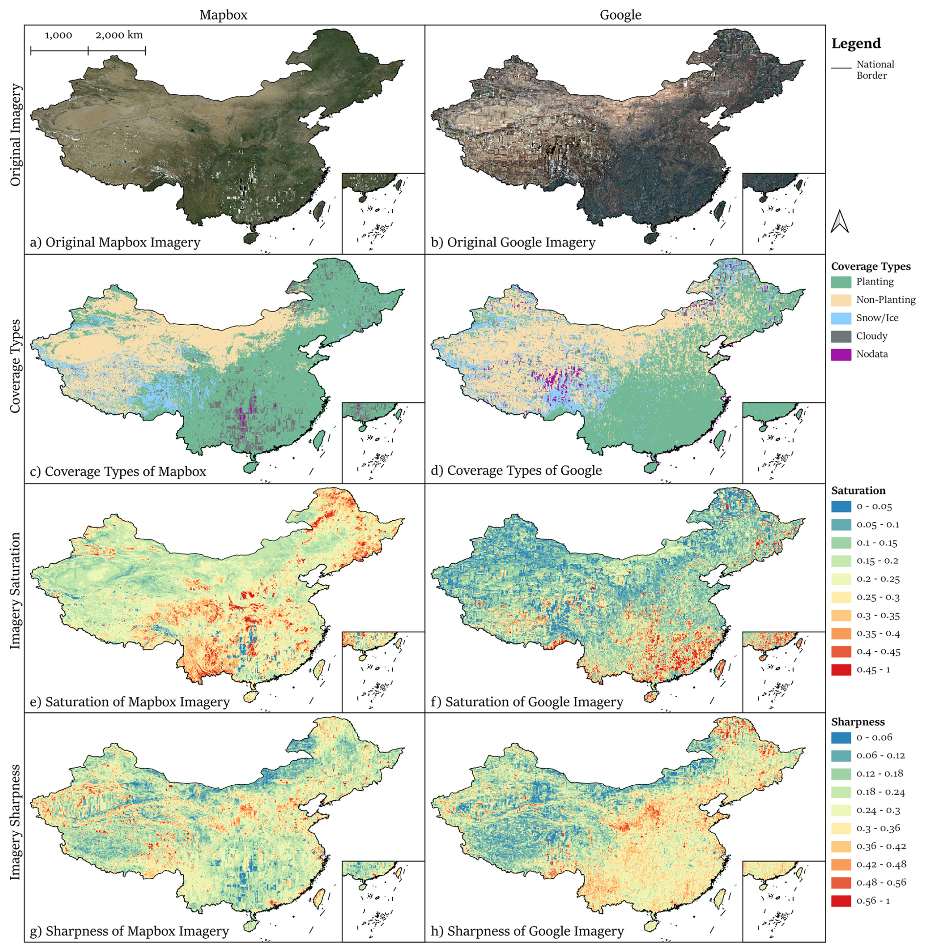
Figure 7 Original Mapbox/ Google Imagery and Image Quality Assessment (IQA). (a) Original imagery from Mapbox; (b) Original imagery from Google; (c) Coverage types of Mapbox imagery; (d) Coverage types of Google imagery; (e) Saturation of Mapbox imagery; (f) Saturation of Google imagery; (g) Sharpness of Mapbox imagery; (h) Sharpness of Google imagery. The HR remote-sensing images in the figure are from ©Mapbox 2023 and ©Google Maps 2023.

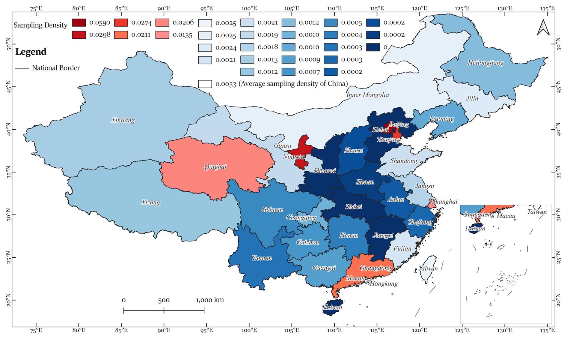
Figure 8 Sampling density for 32 provincial units.

4.2 Active learning for cropland mapping

4.2.1 Sample distribution across provincial units

The AL sampling process was iterated approximately 50 times. To evaluate sample representativeness, sampling density was calculated as the ratio of sampled blocks, including both positive and negative samples, to the total number of blocks within each provincial unit (Fig. 8). Among the 32 provincial units in China, only six provinces including Beijing, Ningxia, Tianjin, Guangdong, Qinghai, and Shanghai exceeded the national average sampling density of 0.0033. Shanghai presented the highest sampling density at 0.0135, whereas Shaanxi, Shanxi, Hebei, Hainan, Henan, Hubei, Anhui, Zhejiang, and Jiangxi exhibited the lowest densities. Low-density provinces were largely located in major grain-producing plains, including the Huang-Huai-Hai Plain and the middle and lower reaches of the Yangtze River. These patterns reflect the interaction between cropland distribution and the AL sampling strategy, where heterogeneous terrain and land cover complexity influenced the number of samples required.

4.2.2 Segmentation model evaluation (Pixel-level)

Four segmentation models: PSPNet, PIDNet, Segformer, and Mask2Former, were evaluated using the validation sample set. Mask2Former achieved the highest IoU (88.73 % vs. 85.10 % for Segformer) and, despite longer training time, showed comparable inference efficiency (Table 6). Given its superior accuracy, especially in detecting smallholder croplands, Mask2Former was selected for this study.

Table 6 Model performance.

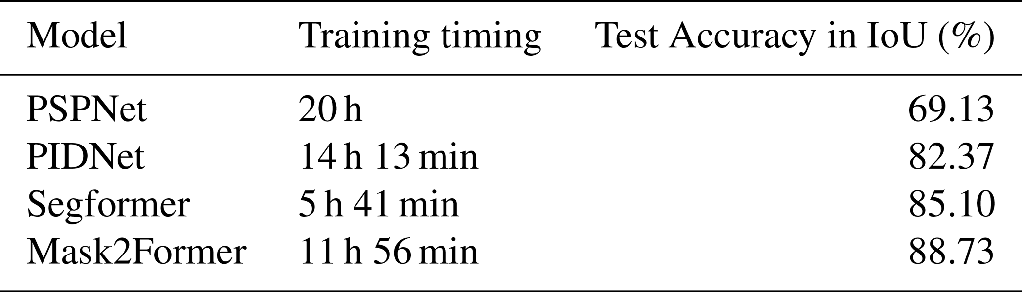
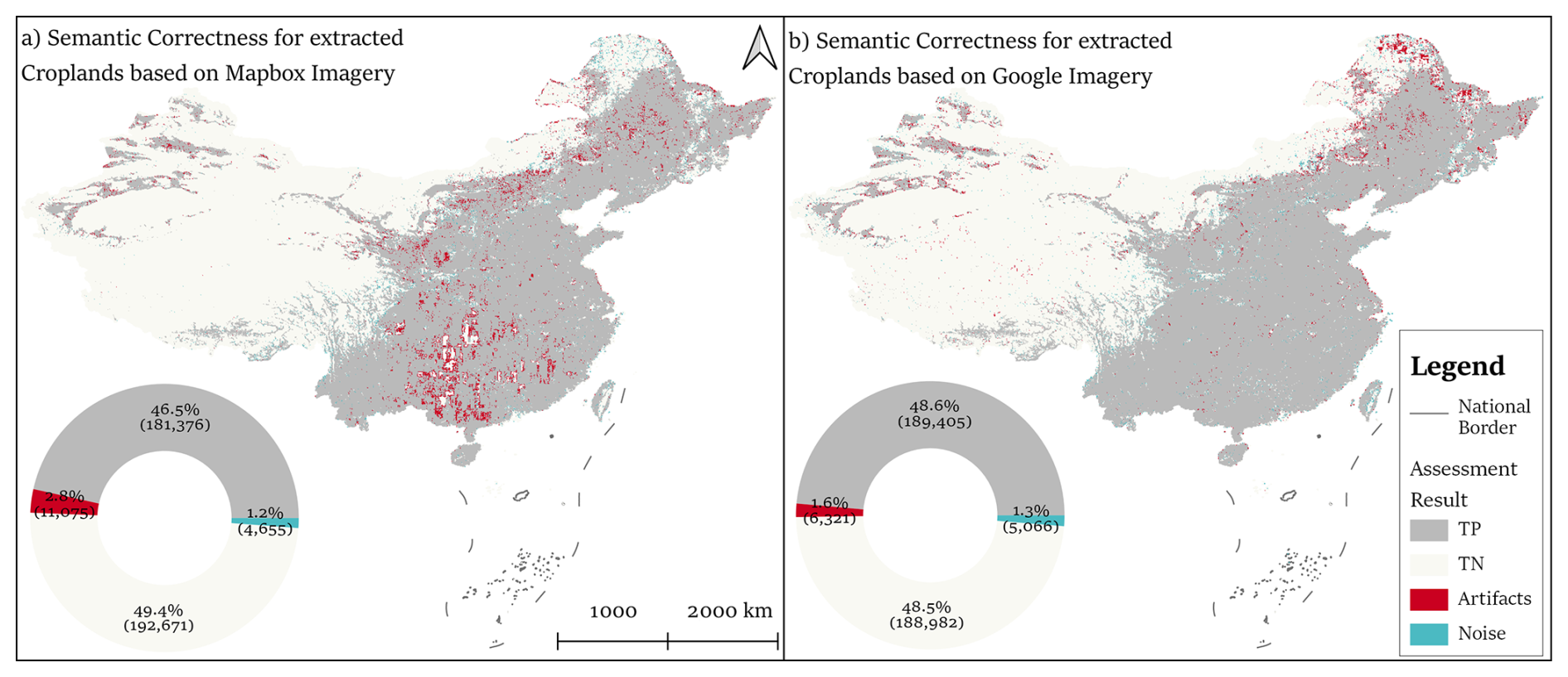
Figure 9 Distribution and statistics of semantic correctness for extracted croplands from (a) Mapbox and (b) Google imagery.

4.2.3 Semantic correctness assessment (Block-level)

Block-level validation assessed the geometric and topological consistency of extracted cropland patches using 16 features list in Table 5. A semantic correctness assessment was conducted using an XGBoost classifier, which quantified the correctness of predicted cropland blocks. The semantic correctness achieved an overall accuracy of 94.3 %, with combined true positive (TP) and true negative (TN) predictions reaching 95.9 % for Mapbox imagery and 97.1 % for Google imagery (Fig. 9). These results demonstrate that both imagery sources provide strong performance for cropland identification, although Mapbox exhibited higher occurrences of Noise and Artifacts relative to Google imagery. Spatially, Artifacts in Mapbox were concentrated in southern mountainous regions affected by Cloudy conditions, while in Google imagery, Artifacts were observed primarily in northeastern China due to Snow/Ice coverage.

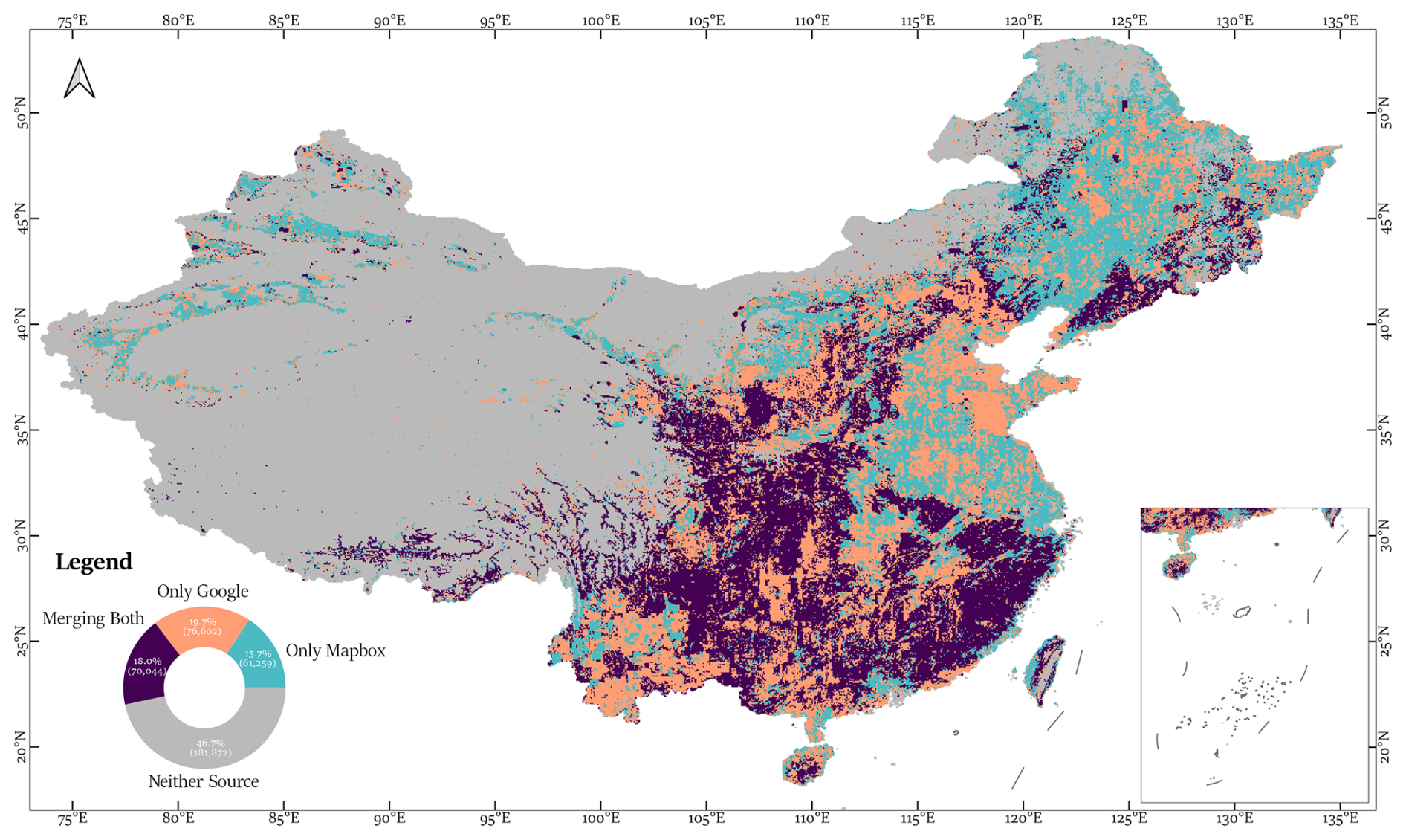
Figure 10 Cropland results integration.

4.2.4 Cropland results integration and feature contribution analysis

The final CropLayer dataset was generated by fusing the cropland extractions from Mapbox and Google. The integration strategy was produced using XGBoost predictions then followed with manual corrections. Integration strategies considered four scenarios: Neither Source, Only Mapbox, Only Google, and Merging Both, accounting for 46.7 %, 15.7 %, 19.7 %, and 18.0 % of total blocks, respectively (Fig. 10).

Single-source regions corresponded mainly to major grain-producing plains, where one imagery source outperformed the other in quality, whereas merged-source regions were located in southern China, terraced landscapes, and mountainous areas. The results indicate that the combination of Mapbox and Google imagery enhances coverage and reliability.

The integration characteristics are summarized as follows:

1. Single Source (Only Mapbox or Only Google): These blocks include major agricultural plains such as the Northeast Plain, North China Plain, central and eastern China, Xinjiang, the Hexi Corridor of Gansu, and Yunnan Province. One imagery source was preferred due to lower quality or coverage limitations in the alternative source.

2. Merged Sources: Blocks where both Mapbox and Google imagery were fused include southern China, the Loess Plateau, eastern Mongolia, terraced landscapes, and Xizang river valleys. Combining sources improved spatial coverage and reduced the impact of cloud, snow, or Nodata blocks.

3. Neither Source: Blocks where neither imagery source was used were mainly located in western China and Inner Mongolia, where persistent low-quality imagery limited cropland extraction.

Overall, the combination of Mapbox and Google imagery, guided by XGBoost predictions and manual refinement, enhanced both the coverage and reliability of the CropLayer dataset across diverse terrains.

Figure 11 Feature importance of Semantic Correctness and Results Integration models.

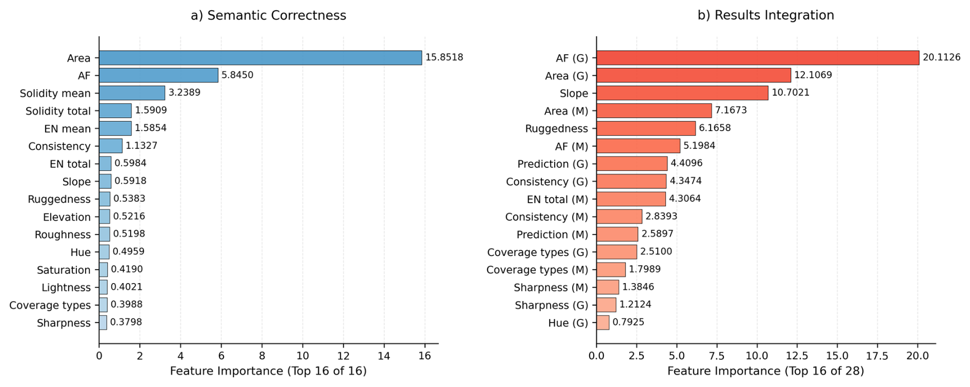
The importance analysis revealed distinct patterns between the two XGBoost models (Fig. 11).

In the Semantic Correctness model, Area and AF were the dominant predictors, followed by Solidity mean, Solidity total, and EN mean, indicating that regional shape and structural complexity are key to identifying reliable cropland predictions.

In the Results Integration model, AF (G), Area (G), Slope, and Area (M) were the most influential features, suggesting that both spatial extent and topographic context play critical roles in integrating the two datasets.

Among non-topographic features, IQA variables (e.g., Sharpness, Hue, Lightness) exhibited moderate importance, highlighting the influence of image quality in determining which data source provides the more reliable prediction.

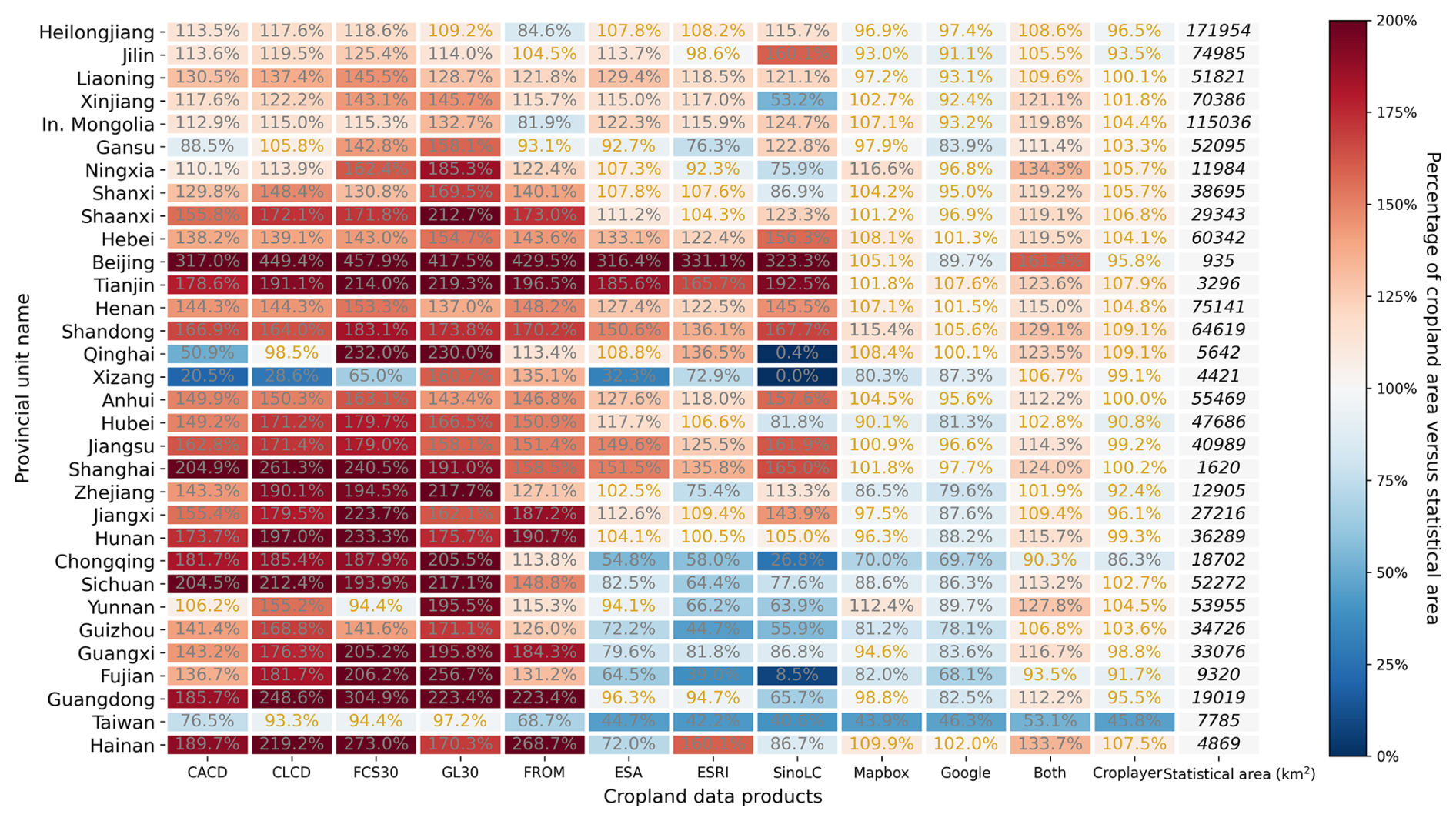
Figure 12 Percentage of cropland area versus statistical area (PCS) of eight existing datasets and four extraction scenarios (Only Mapbox, Only Google, Merge Both, and Selected Integration). “In. Mongolia” denotes Inner Mongolia.

4.2.5 Area validation (Provincial-level)

Provincial-level area validation evaluated the compliance of cropland extractions with AL stop criteria. Figure 12 compares provincial cropland areas derived from four extraction scenarios (Only Mapbox, Only Google, Complete Integration, and Selected Integration) with TNLS statistical records.

For single sources, Mapbox did not meet the area-based stop criteria in Zhejiang, Chongqing, Guizhou, Fujian, and Taiwan, whereas Google failed in Chongqing and Taiwan. According to the AL stop criteria, provincial cropland areas were required to reach at least 80 % of the corresponding statistical record. When the threshold was not achieved, additional sampling and retraining were performed up to three iterations. Only in Chongqing and Taiwan did the cropland area remain below the required threshold after three rounds of additional sampling, and these provinces were therefore excluded from further iterations.

Figure 13 IoU of 8 existing cropland datasets versus CropLayer.

4.3 Multi-level evaluation of CropLayer dataset

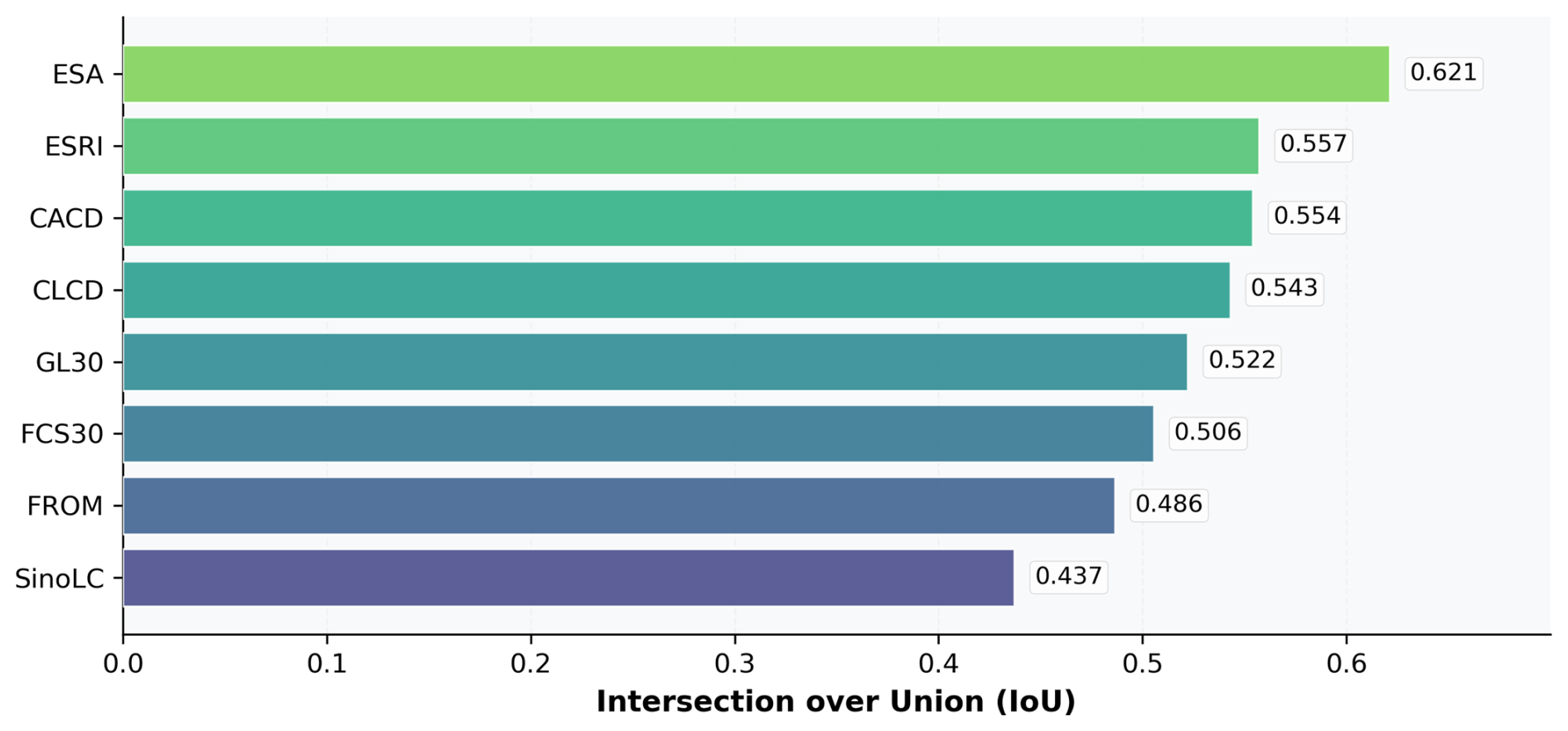
4.3.1 Pixel-level evaluation (IoU)

CropLayer was compared with eight publicly available cropland datasets using the IoU. ESA exhibited the highest IoU (0.62), followed by ESRI (0.56) and CACD (0.55), while FROM and SinoLC demonstrated the lowest agreement (0.49 and 0.44, respectively) (Fig. 13). Overall, the pixel-level comparison suggests a moderate degree of agreement among existing products in terms of cropland extent.

These results motivate a finer-scale investigation into where and why differences occur, which is addressed through block-level structural analysis in the next section.

4.3.2 Block-level evaluation (Area Fraction, Edge Density, Slope)

The block-level comparison is performed using three block-based metrics: AF, ED, and Slope median. For each dataset, deviations from CropLayer were quantified according to Eq. (6). To simplify the presentation, we focused on the four datasets with the highest IoU values (ESA, ESRI, CACD, and CLCD), which also share the most similar cropland definitions with CropLayer, as shown in Fig. 4. In these deviation maps, red indicates overestimation and blue indicates underestimation relative to CropLayer, with color intensity representing the magnitude of deviation.

The AF results show that all four datasets maintain low deviation in the major agricultural plains of Northeast, North, and the middle-lower Yangtze regions, where cropland patterns are extensive and homogeneous. Differences are mainly concentrated in mountainous and hilly areas, where field structures are more fragmented. Specifically, CACD and CLCD show widespread overestimation in several regions, while ESA and ESRI exhibit smaller deviations. Nevertheless, ESA tends to overestimate cropland near arid and semi-arid regions (Inner Mongolia, Gansu, Qinghai, and Xinjiang) as well as around urban and water areas, whereas ESRI shows consistent underestimation across much of southern China.

For ED, patterns differ slightly: CACD shows local overestimation in northern pastoral zones but underestimation in most other areas, similar to CLCD and ESRI. ESA generally underestimates ED, though to a lesser degree, with localized overestimation near water bodies and built-up zones. These results indicate that coarse-resolution datasets tend to simplify cropland boundaries, merging adjacent patches and reducing edge complexity, an effect particularly visible in heterogeneous terrain.

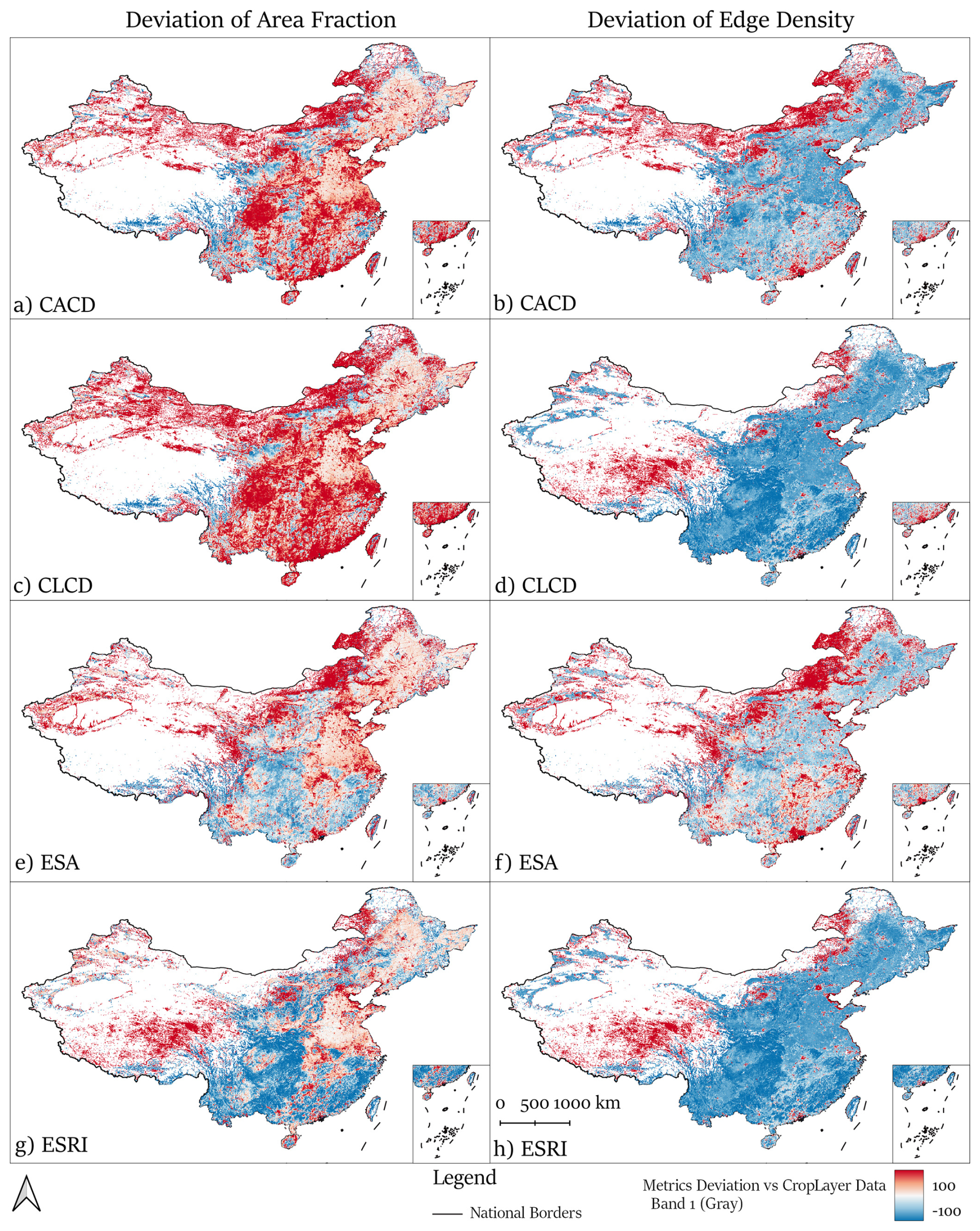
Figure 14 Spatial distribution of deviation in Area Fraction and Edge Density for CACD, CLCD, ESA, and ESRI relative to CropLayer.

Figure 15 Histogram of deviation versus slope for CACD, CLCD, ESA, and ESRI.

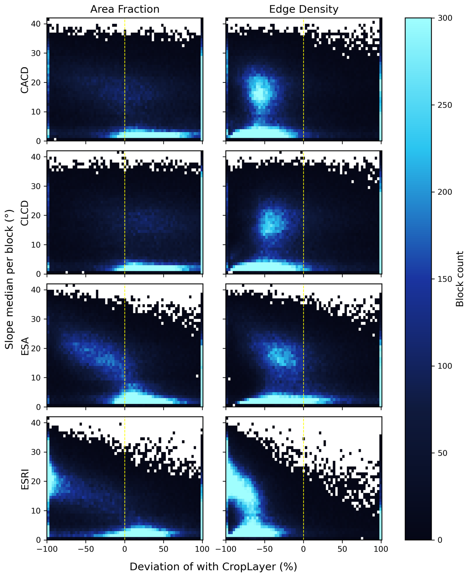
To examine terrain influences, we analyzed the slope conditions of all blocks with AF > 0.1 for each dataset. Figure 15 shows the histogram of deviations with respect to slope median, where the bin counts reflect the joint distribution of slope and deviation percentage. Among all datasets, ESRI exhibits the widest slope range and the strongest overall deviation in both AF and ED, indicating greater inconsistency across diverse terrain. For CACD, CLCD, and ESA, the most pronounced ED underestimation occurs in the roughly 10–25° slope range, corresponding to terraced and hilly cropland. The degree of underestimation decreases progressively from CACD to CLCD to ESA, consistent with their spatial patterns in Fig. 14. In contrast, deviations over flatter regions mainly correspond to extensive plains where differences arise from broader underestimation patterns rather than local terrain effects.

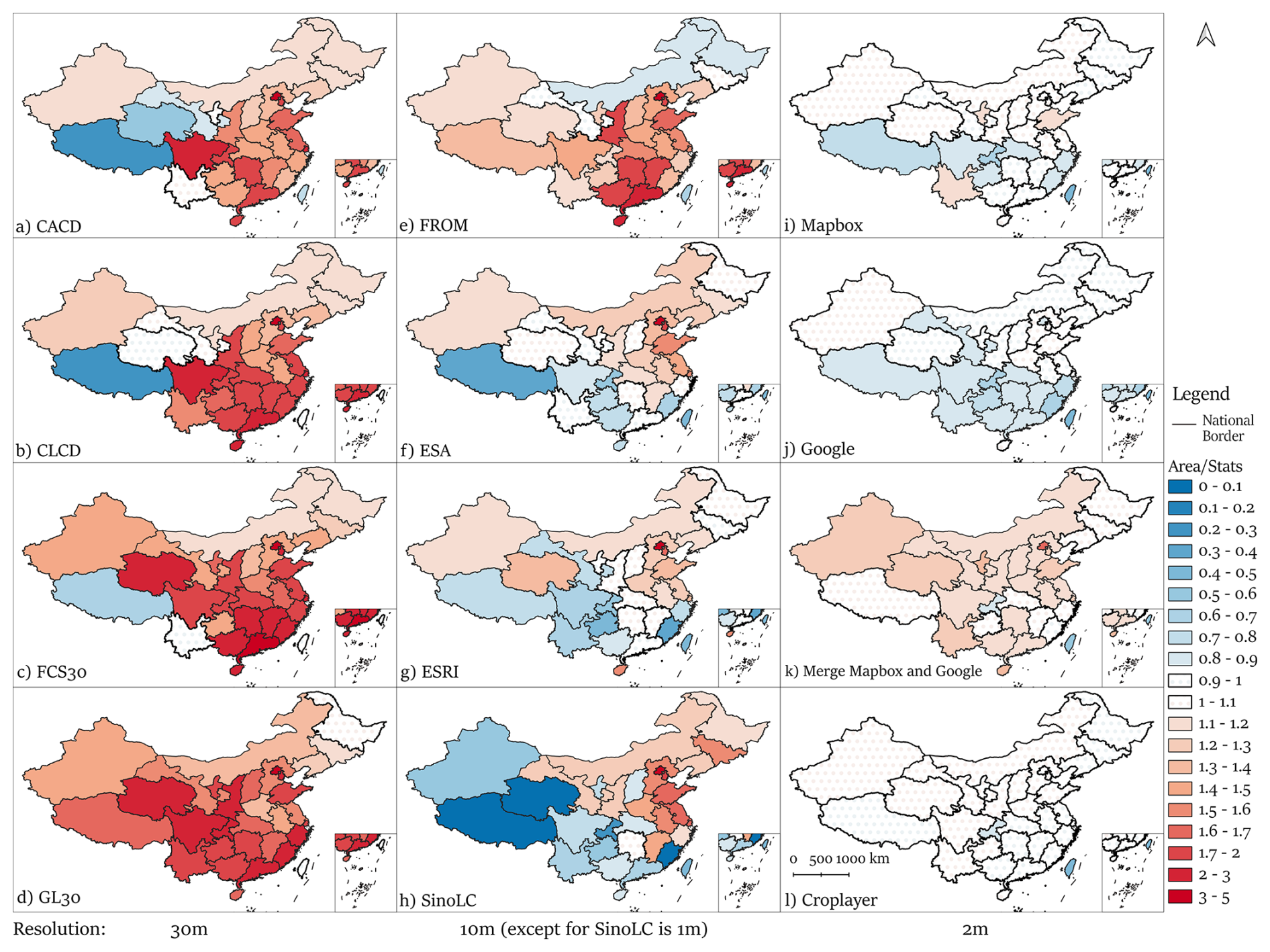
Figure 16 PCS distribution of eight existing datasets and four extraction scenarios (Mapbox, Google, Merge both, and Selected Integration).

4.3.3 Provincial-level evaluation (Area Consistency with TNLS)

CropLayer exhibited strong consistency with TNLS statistics, with 30 of 32 provinces within ± 10 % of reported cropland areas (Fig. 16). Other datasets achieved this in far fewer provinces: ESA and ESRI in 9, CLCD and FROM in 2, and the remaining datasets in only 1.

Northern provinces generally had consistent or slightly higher cropland estimates relative to TNLS, while southern provinces showed greater variability due to complex topography, heterogeneous land cover, and mixed cropland-forest or cropland-urban regions. This confirms CropLayer's reliability for representing regional-scale agricultural distributions.

5 Discussion

5.1 Impact of the image quality

Image quality directly affects the accuracy of cropland mapping. Our results show that Mapbox and Google datasets have similar proportions of high-quality imagery (82.8 % vs. 82.1 %), but their low-quality categories exhibit distinct spatial distributions: Mapbox is more affected by Cloudy and Nodata blocks in southern China and the northeast, whereas Google experiences more Snow/Ice and Cloudy blocks in the Qinghai-Xizang Plateau and northeast regions. This complementary pattern provides potential advantages for multi-source integration.

Theoretically, substituting low-quality imagery from one source with high-quality imagery from the other could reduce the overall low-quality rate to 6.8 %. However, in this study, we did not implement such a block-replacement strategy; instead, we independently extracted cropland from each dataset and applied integration to mitigate low-quality regions. Therefore, the 6.8 % images serve as a quantitative indicator of complementary potential rather than an achievable accuracy level. Notably, higher data quality does not always guarantee better extraction performance, as some lower-quality images can still contain valuable cropland information; for example, Non-Planting season images sometimes capture tillage textures that help delineate paddy fields more clearly.

Despite the five-category IQA performed in this study, certain challenging issues remain difficult to detect automatically. Some anomalies extend beyond three predefined low-quality categories. For instance, a single image block often contains multiple stitched scenes, generating false edges that the current ResNet-based IQA method fails to reliably identify. Future approaches incorporating models with stronger semantic comprehension, such as Transformer-based architectures or CLIP (Radford et al., 2021) could improve the detection of such anomalies and further enhance extraction accuracy.

Overall, this study highlights that integrating multiple complementary data sources, combined with quality assessment and result fusion, provides a more balanced approach to ensuring spatial coverage and mapping accuracy than relying on a single high-resolution imagery source. This strategy is particularly necessary for regions with complex cropland distribution and pronounced climate variation, such as China, and provides a useful reference for high-resolution cropland mapping in other regions.

5.2 Cropland mapping and active learning

Accurate large-scale cropland mapping is influenced by multiple factors, particularly the semantic definition of cropland and the spatial resolution of input imagery. Our provincial-level results illustrate these two failure modes. Taiwan is an example of definitional mismatch: official statistics include perennial woody crops (for example orchards), while CropLayer is focused on annual herbaceous croplands, which produces an apparent underestimation. Chongqing exemplifies the limits of spatial resolution: the prevalence of extremely small plots, where over 80 % of single cropland parcels are below 1 mu (approximately 0.067 ha), combined with steeply sloped terrain. This make reliable delineation difficult even at 2 m resolution, suggesting that sub-meter imagery would be needed to substantially improve performance in the most complex mountain farming systems.

AL proved to be a highly sample-efficient strategy but required substantial iterative effort. Out of roughly 779 554 blocks from two imagery sources we labeled 366 positive and 761 negative samples during AL, a sampling fraction of about 0.14 % and a labeling ratio of 0.05 %. For comparison, the systematic semantic-correctness validation collected 7754 samples. AL thus dramatically reduced the number of costly human labels required to reach high performance, but it demands repeated cycles of sample selection, annotation, retraining, and error inspection; this is computationally and labor intensive and explains, in practice, why we limited the mapping to 2 m imagery rather than pursuing 0.6 m across the entire country.

The three-level validation scheme was essential for controlling AL and avoiding overfitting. Pixel-level metrics alone can be misleading: a model trained in Guangdong reached an internal IoU of 89.65 % but fell to below 20 % when applied nationally, demonstrating strong local overfitting. To prevent this, we adopted explicit AL stop criteria: pixel-level IoU not below 85 %, block-level semantic correctness not below 85 %, and provincial area agreement at least 80 % of the official statistic (either the Mapbox or Google-derived area met this threshold). If a province failed the area criterion, up to three additional AL iterations were attempted; if performance did not improve and imagery quality was persistently poor, the province was skipped. Using these multi-scale thresholds ensured that the model improved not only on pixel-wise accuracy but also on semantic structure and regional total area, and it provided a concrete, operational termination rule for the costly AL loop.

The semantic correctness assessment, implemented with an XGBoost classifier, was effective in identifying problematic blocks and guiding supplementary sampling. The classifier achieved an overall accuracy of 94.3 % with semantic correctness (combined TP and TN) rates achieved to 96.5 % (95.9 % for Mapbox and 97.1 % for Google). These metrics validated that both imagery sources are strong for cropland detection while revealing systematic differences: Mapbox showed more noise and artifact patterns in southern, cloud-prone mountainous areas, and Google showed more artifacts tied to snow and ice in the northeast. The semantic-correctness signal therefore provided a practical and scalable proxy for block-level quality beyond what pixel IoU can reveal.

Beyond performance evaluation, the feature importance analysis offered valuable insight into the model's decision process. The dominance of Area and AF aligns with the spatial distribution patterns observed in Fig. 10, where approximately 46.7 % of the blocks contain no cropland. These features directly capture cropland presence and proportion, thus serving as the most fundamental predictors. The significant roles of Solidity and EN in the Semantic Correctness model reflect their sensitivity to field shape regularity and boundary complexity, which effectively distinguish realistic cropland patches from artifacts. In contrast, the Results Integration model highlights the importance of Slope and Ruggedness, indicating that topographic variability is a major determinant when fusion of Mapbox and Google-derived results. Moreover, the relatively higher importance of IQA features in this stage suggests that image quality strongly affects the reliability of the integrated outputs. Overall, the importance ranking aligns well with empirical expectations, confirming that the model's decisions are physically and contextually interpretable.

5.3 Comparison with existing datasets: strengths and limitations of CropLayer

CropLayer achieves substantially higher agreement with provincial statistics than the other evaluated products: 30 of 32 provinces within ± 10 %. This high level of regional consistency indicates that the combined use of HR imagery and AL, constrained by statistical area checks, produces a reliable national product for policy and statistical applications.

However, provincial agreement masks important spatial heterogeneity. Pixel-level IoU comparisons show only moderate agreement between CropLayer and other datasets (IoU range roughly 0.44 to 0.62, ESA highest). These moderate values reflect two main issues. First, many existing products use coarser imagery (10–30 m) and rely heavily on spectral and temporal signatures, while CropLayer leverages spatial morphology, texture, and color available at 2 m. Second, semantic definitions differ across products: some include perennial woody crops, others do not, which directly affects area comparisons.

Block-level metrics reveal where and why coarse-resolution products fail. AF and ED deviations between CropLayer and other datasets concentrate in hilly and mountainous zones such as the Yunnan-Guizhou Plateau, the margins of the Sichuan Basin, and parts of southern Gansu. In these areas, medium- and coarse-resolution maps tend to merge small plots and simplify boundaries, producing higher AF and lower ED. The slope-deviation analysis shows that edge-density underestimation is most pronounced in the 10–25° slope band, which corresponds to terraces and dissected hillslopes. This terrain-linked structural bias explains much of the regional divergence and demonstrates the particular value of 2 m imagery for preserving morphological realism in complex landscapes.

For national or provincial statistics and many regional planning applications, CropLayer offers clear advantages over 10–30 m products. For field-level management, especially in highly fragmented mountainous regions, further gains will require sub-meter imagery and/or instance segmentation, and these improvements come with substantially higher labeling and compute costs.

5.4 Potential use of the data

The CropLayer dataset provides a robust and transparent foundation for diverse agricultural and environmental applications, ranging from crop distribution mapping and growth monitoring to yield estimation and disaster impact assessment. Its precise delineation of cropland boundaries ensures strong consistency with provincial statistical values and facilitates seamless integration into broader analytical frameworks. The potential uses and advantages of CropLayer can be summarized as follows:

1. Enhanced data comparability and transparency

   CropLayer achieves high consistency with official provincial statistics while relying exclusively on publicly accessible imagery sources, ensuring reproducibility and open scientific collaboration. This transparency supports cross-study comparability and encourages data-sharing across the agricultural and environmental research communities. Furthermore, derived products such as crop yield estimates based on CropLayer maintain statistical coherence with existing datasets, enabling harmonized use in national assessments and multi-model intercomparisons.

2. Advancing agricultural modeling and AI-based analytics

   Accurate cropland delineation provides a reliable spatial foundation for downstream analyses, including classification of rainfed, irrigated, and paddy croplands, as well as finer subcategories (Salmon et al., 2015). The nationwide coverage and 2 m resolution of CropLayer also offer essential training data for agricultural foundation models (Li et al., 2024) and large-scale knowledge systems (Yang et al., 2024), supporting progress in predictive modeling of crop growth, yield estimation, and environmental impact assessment. By linking high-quality geospatial data with advanced machine learning frameworks, CropLayer contributes to the development of more generalized and interpretable agricultural AI models.

3. Improving land-cover and environmental analyses

   By more accurately delineating cropland areas, CropLayer reduces misclassifications in adjacent land-cover categories such as forests, water bodies, and built-up regions. This improvement enhances the reliability of multi-class land-cover datasets, which are crucial for ecological monitoring, environmental management, and urban planning (Chen et al., 2022). The dataset thus plays an important role not only in agricultural analysis but also in refining the overall quality and interpretability of Earth observation-based land-cover products.

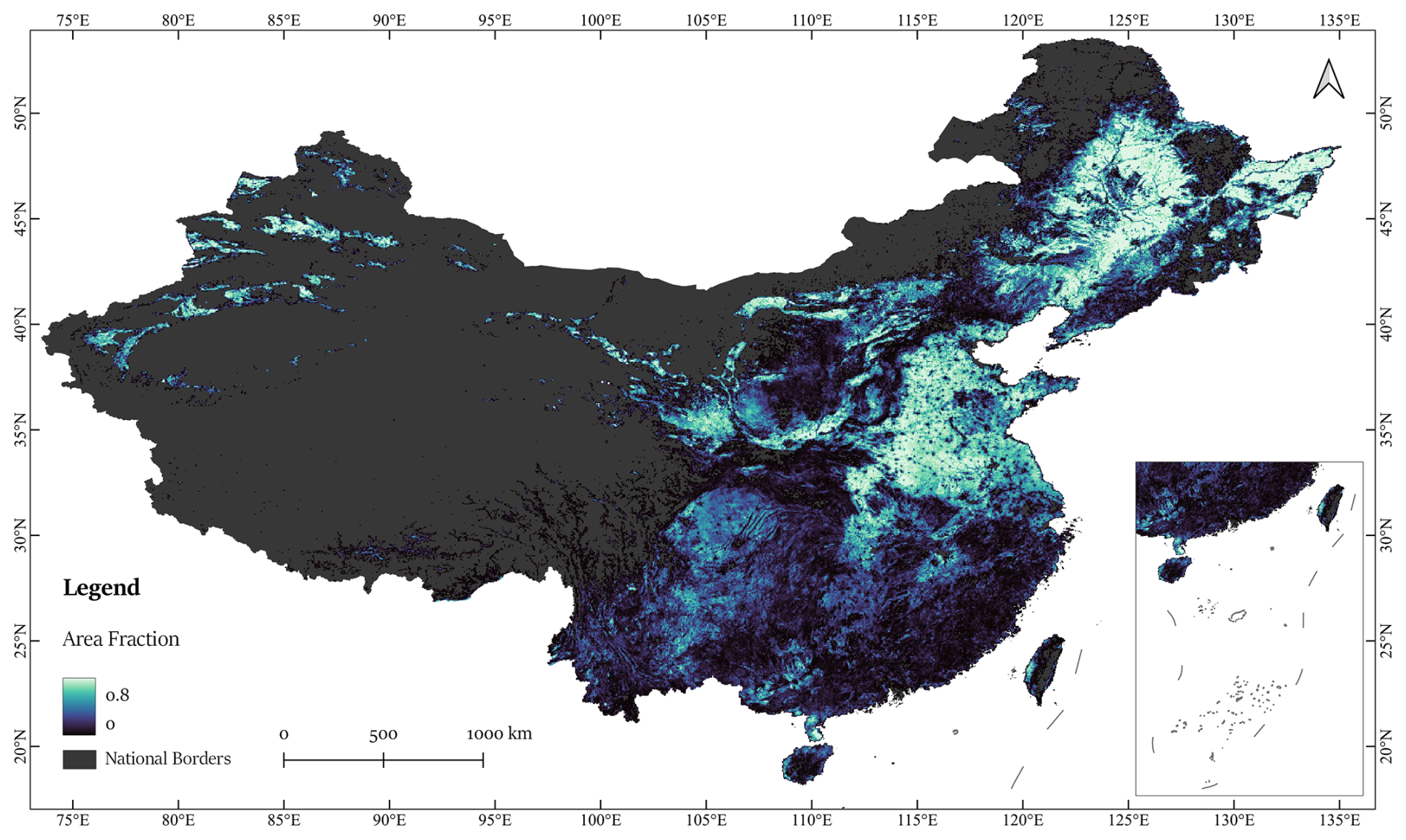
Figure 17 National distribution of cropland in China for the year 2020, as depicted by Area Fraction of the CropLayer dataset.

5.5 Limitations and future directions

Despite its advantages, several limitations of this study highlight directions for future improvement. CropLayer currently employs semantic segmentation, which effectively identifies cropland extents but does not distinguish individual fields. This limits detailed analyses such as per-field area statistics and parcel-based management. Incorporating instance segmentation into future versions would allow explicit field boundary detection, significantly enhancing the dataset's applicability for agricultural monitoring and precision farming.

Although CropLayer demonstrates strong agreement with provincial statistics, the lack of comprehensive municipal- and county-level cropland data prevents fine-scale validation. While provincial estimates are reliable, discrepancies exist within provinces, particularly near rapidly urbanizing zones where overestimation occurs due to outdated imagery or mixed land use. These biases underscore the need for more frequent imagery updates and improved access to localized agricultural statistics. As noted by (Xian et al., 2009), rapid urban expansion can quickly alter land cover, and timely updates are essential to maintain mapping accuracy.

Another important direction is to extend CropLayer into a multi-temporal framework. Current limitations arise from the uneven refresh cycles of Mapbox and Google imagery: urban regions are typically updated every 1–2 years, whereas remote rural areas may not be refreshed for more than five years. This temporal inconsistency complicates annual mapping but can be mitigated once a stable baseline is established. Future work should integrate imagery selection using image quality assessment (IQA), apply the established segmentation and fusion framework to incremental updates, and incorporate newly available open high-resolution datasets, such as ESA's PhiSat-2 (https://earth.esa.int/eogateway/missions/phisat-2, last access: 26 November 2025). These developments will enable more frequent and accurate cropland monitoring, advancing both scientific research and agricultural policy support.

5.6 The CropLayer dataset: a national overview

Figure 17 illustrates the national cropland distribution in 2020 based on CropLayer block-level AF, highlighting dense plains in eastern China and fragmented croplands in other mountainous, hilly and arid regions.

6 Data availability

The CropLayer China 2020 dataset generated in this study is available on Zenodo: https://doi.org/10.5281/zenodo.14726428 (Jiang et al., 2025). The dataset is provided in Shapefile (.shp) format, with each file representing the cropland extent within a county-level administrative region in China. To ensure clarity and avoid duplicate names, file names follow the format cf_city_county (in Chinese). All county-level files are organized by province, and each province is distributed as a compressed archive (.tar.gz). Additional datasets used in this study are described in Sect. 2, along with their respective download links.

7 Conclusion

Existing public cropland datasets in China exhibit substantial spatial inconsistencies. To address this, we developed CropLayer, a 2 m-resolution cropland map for 2020, generated through a three-stage workflow: (1) image quality assessment to compensate for missing metadata; (2) active learning–based extraction using Mask2Former, evaluated by a three-level validation scheme at pixel, block, and regional scales; and (3) XGBoost-based integration of Mapbox and Google imagery.

CropLayer achieves a pixel-level accuracy of 88.73 %, a block-level semantic correctness of 96.5 %, and strong agreement with official statistics, with 30 out of 32 provincial units showing area estimates within ± 10 % deviation. In contrast, only 1–9 provinces meet this standard across eight existing datasets. The 2 m resolution enables precise delineation of cropland boundaries, particularly in fragmented and topographically complex regions that are often oversimplified in coarser products.

The dataset serves as a transparent and reproducible benchmark for agricultural monitoring, yield estimation, and land-use studies, and the workflow provides a generalizable solution for producing high-accuracy cropland maps in regions characterized by complex landscapes.