HIStory of LAND transformation by humans in South America (HISLAND-SA): annual and 1 km gridded data for soybean, maize, wheat, and rice (1950–2020)

South America is a global hotspot for land use and land cover (LULC) change, marked by dramatic agricultural land expansion and deforestation. While previous studies have documented land use and land cover changes in South America over recent decades, there is still a lack of spatially explicit and time-series maps of crop types that capture shifts in crop distribution. Therefore, developing high-resolution, long-term, and crop-specific datasets is crucial for advancing our understanding of human–environment interactions and for assessing the impacts of agricultural activities on carbon and biogeochemical cycles, biodiversity, and climate. In this study, we integrated multi-source data, including high-resolution remote sensing data, model-based data, and historical agricultural census data, to reconstruct the historical dynamics of four major commodity crops (i.e., soybean, maize, wheat, and rice) in South America at an annual timescale and 1 km × 1 km spatial resolution from 1950 to 2020. The results showed that soybean and maize cultivation expanded rapidly in South America by encroaching on other vegetation (i.e., forest, pasture/rangeland, and unmanaged grass/shrubland) over the past 70 years, whereas wheat and rice areas remained relatively stable. Specifically, soybean is one of the most dramatically expanded crops, increasing from essentially zero in 1950 to 48.8 Mha in 2020, resulting in a total loss of 23.92 Mha of other vegetation. In addition, the area of maize increased by a factor of 2.1 from 12.7 Mha in 1950 to 26.9 Mha in 2020. The newly developed crop type dataset provides important insights for assessing the impacts of cropland expansion on crop production, biodiversity, greenhouse gas emissions, and carbon and nitrogen cycles in South America. Moreover, these data are instrumental for developing national policies, sustainable trade, investment, and development strategies aimed at securing food supply and other human and environmental objectives in South America. The datasets are available at https://doi.org/10.5281/zenodo.14002960 (Xu et al., 2024).

1 Introduction

South America is of critical importance due to its substantial contribution to global agriculture, which is essential for meeting the world's growing food demand (Ceddia et al., 2014; Hoang et al., 2023). Cropland expansion in this region has been a significant driver of land use transformation, particularly through deforestation, with profound effects on ecosystems and biogeochemical processes (Song et al., 2021; Zalles et al., 2021). As one of the main types of land use and land cover (LULC), cropland plays a crucial role in supporting human nutritional needs and ensuring food security (He et al., 2017; Yu and Lu, 2017). However, to meet the growing demand for food and fiber driven by population growth and consumption patterns, cropland has increasingly encroached on natural vegetation (Winkler et al., 2021). Additionally, economic and policy factors have reshaped crop cultivation structures across the region (Cheng et al., 2023; Mueller and Mueller, 2010; Song et al., 2021). These changes are driven by a combination of trade dynamics, investment flows, and market concentration (Boyd, 2023; Clapp, 2021). As a result, the transformation of crop types has occurred, weakening the resilience of agroecosystems and contributing to biodiversity loss (Frison et al., 2011; Renard and Tilman, 2019). In response to these challenges, the international community has increasingly emphasized the need to align agricultural systems with climate mitigation and food security goals (ICJ, 2025). Therefore, an improved understanding of the spatial distribution and historical dynamics of crop types is urgently needed to assess the impacts of cropland expansion and crop pattern shifts across South America. Such insights are crucial for evaluating the environmental and socioeconomic consequences of cropland expansion, particularly in terms of its impact on climate, ecosystems, and food security.

Agriculture in South America has experienced significant changes driven by agricultural policies, socioeconomic shifts, and technological innovations after the 1950s (Altieri, 1992; Ceddia et al., 2014; Zalles et al., 2021). These changes have not only reshaped regional economies, as in other historical periods of agrarian reform, but also been justified by global food security goals, alongside such other important drivers as trade relationships, investors, subsidies, and debt-serving goals (Boyd, 2023; OAS, 2024). In this context, crop cultivation has shifted from traditional crops to high-yield and high-demand commodity crops, reflecting both the increasing global demand for food and fuel and the urgent need to enhance agricultural efficiency and yields (Garrett et al., 2013; Meyfroidt et al., 2014). Specifically, the major commodity crops (i.e., maize, soybean, wheat, and rice) have become the core of agricultural production in South America (FAO, 2020). The cultivation of these crops has not only significantly boosted food production in the region but also secured a strong position for many producers in the global food market. After the 1950s, countries in South America (e.g., Bolivia, Brazil, Chile, Colombia, Ecuador, and Peru) undertook land reforms to reduce land concentration and promote agricultural production (De Janvry et al., 1998), which significantly affected land use outputs and efficiency and laid a substantial foundation for the development of agriculture (De Janvry et al., 1998; Munoz and Lavadenz, 1997). After the 1980s, neoliberal economic reforms were further carried out in South America, accelerating the ongoing agricultural modernization (Chonchol, 1990) and greatly facilitating the cultivation of soybeans by eliminating price controls and export restrictions on agricultural products (Campos Matos, 2013). Since the 2000s, soybean production has continued to grow dramatically due to global demand, technological advances, economic subsidies, and other supportive policies (de LT Oliveira, 2017; Song et al., 2021). This growth has further bolstered the expansion of maize cultivation, driven by the promotion of maize–soybean cropping systems; the adoption of direct-seeding, no-tillage practices; and double cropping (Klein and Luna, 2022). In comparison, the area under wheat and rice cultivation has remained relatively stable. Although there is a growing demand for wheat, its market price is less fluctuating, leading farmers, farm managers, and investors to prefer crops with higher market returns (Erenstein et al., 2022). Meanwhile, rice primarily serves domestic demand rather than being export-oriented (Dawe et al., 2010). Despite government reports and documents that have recorded changes in the dynamics of agriculture in South America over the past few decades, there is still a lack of spatially explicit and time-series maps of historical crop types that reflect changes in crop distribution. This deficiency makes it difficult to fully understand the spatial and temporal evolution of major commodity crops and hinders understanding of their impacts on environmental changes.

Many efforts have produced commodity crop maps at regional or global scales. For example, datasets such as the Spatial Production Allocation Model (SPAM) (Yu et al., 2020), M3 (Monfreda et al., 2008), and CROPGRIDS (Tang et al., 2023) offer valuable solutions by providing detailed crop type information based on census data and spatial allocation algorithms. SPAM, for instance, provides data on crop area, yield, and production for 42 major crops at a spatial resolution of 5 arcmin under four farming systems. However, these datasets have a coarse spatial resolution and are available for only a few years, which makes it challenging to accurately characterize the spatial–temporal distribution of crop types at finer scales (Becker-Reshef et al., 2023; Ye et al., 2024). In contrast, with the continuous evolution of remote sensing technologies, high-resolution data have increasingly been used to develop fine-scale crop type maps. For example, Song et al. (2021) developed annually updated soybean maps with a 30 m resolution for South America from 2000 to 2023 using all Landsat and MODIS images and a probability sample of continental field observations. MapBiomas also provides high-resolution crop type maps for Argentina, Brazil, and Uruguay, covering the period from 1985 to the present (De Abelleyra et al., 2020; Petraglia et al., 2019; Souza and Azevedo, 2017). However, these existing datasets are available only at partial national or local scales, cover only a single crop type, or lack rigorous validation. Furthermore, most remote sensing data date back only to 1985, making it challenging to depict crop dynamics further back. Therefore, it is imperative to develop high-resolution and time-series crop type data for driving terrestrial ecosystem models to quantify the impact of crop dynamics on ecosystems and climate. Such a dataset will draw on innovations in earth science and data use to contribute to related fields that address the “advance of the agricultural frontier” in South America and its implications for human–environmental interactions (Liu et al., 2007; OAS, 2024).

In this study, we aim to develop an annual and 1 km crop-specific (i.e., soybean, wheat, maize, and rice) gridded dataset for South America from 1950 to 2020 by integrating agricultural census data and remote-sensing-based and model-based crop type distribution maps. This study focuses on understanding how the spatial–temporal patterns of these four commodity crops have evolved over the past seven decades and how these changes have influenced land use transitions in South America. The dataset is designed to support research on agricultural land use change, its ecological impacts, and food security, offering insights into the effects of agricultural expansion on deforestation, biodiversity loss, and greenhouse gas emissions. It provides critical information for policymakers, researchers, and stakeholders engaged in sustainable agriculture, thereby assisting in the development of strategies that balance agricultural production with environmental conservation.

2 Materials and method

2.1 Study area

This study aims to reconstruct crop type (i.e., soybean, wheat, maize, and rice) data at annual and 1 km resolution from 1950 to 2020 in South America using the high-resolution remote-sensing-based crop type data, model-based crop type data, and historical agricultural census data. We focused on generating data for the 13 countries in South America, including Argentina, Bolivia, Brazil, Chile, Colombia, French Guiana, Ecuador, Guyana, Paraguay, Peru, Suriname, Uruguay, and Venezuela (Fig. 1). Considering the data availability, we excluded the Falkland Islands and South Georgia and the South Sandwich Islands. We used GADM version 4.1 Level 1 administrative units (i.e., province level) as the basic unit for this study, which included a total of 243 administrative units (Table S1 in the Supplement). Moreover, to maintain consistency with historical agricultural census data, some administrative units were regrouped and merged for area calibration. Specifically, we merged Buenos Aires and Ciudad de Buenos Aires in Argentina; Bogotá D.C. and Cundinamarca in Colombia; Asunción and Central in Paraguay; Callao, Lima, and Lima Province in Peru; and all regions together in French Guiana. Ultimately, a total of 237 administrative units were used to reconstruct historical cropland density and crop type data (Table S1).

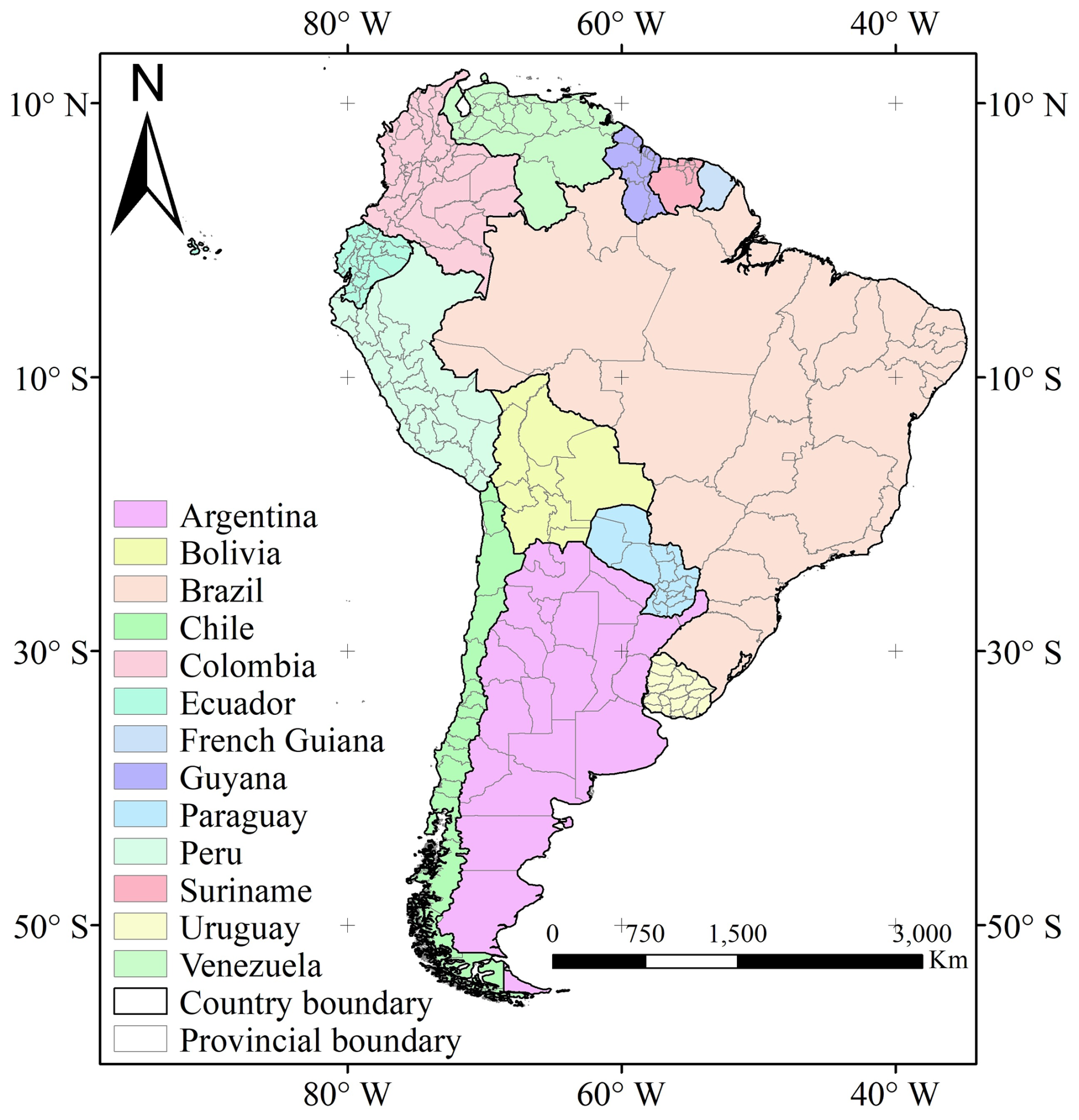
Figure 1 Geopolitical and administrative divisions of South America.

2.2 Workflow

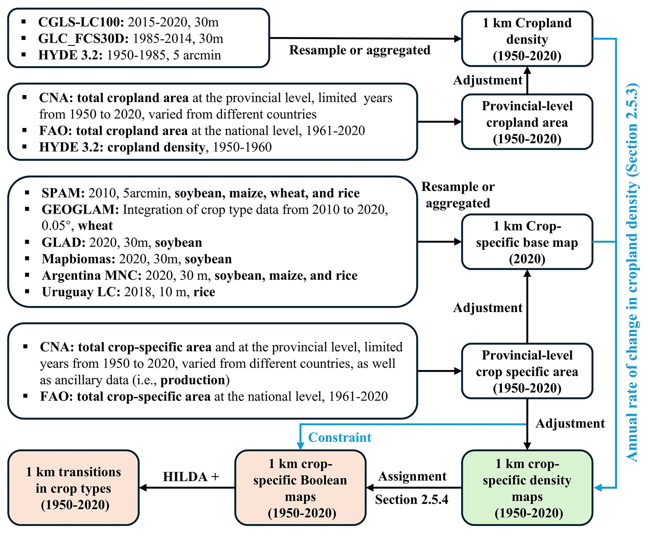
The structure of this paper includes three main sections (Fig. 2). The first section provides a detailed description of the input data and methods. The second section performs a comprehensive analysis of the spatial and temporal characteristics of four major commodity crops over the past seven decades. The third section compares the results of this study with other existing datasets and analyses the driving forces and uncertainties associated with the reconstructed data.

Figure 2 The flowchart of this study. CNA refers to Census National Agriculture.

2.3 Input data

2.3.1 Gridded datasets and preprocessing

In this study, we used both remote-sensing-based and model-based LULC and crop type data to generate cropland density maps and crop type base maps in South America. As shown in Table 1, CGLS-LC100, GLC_FCS30D, and HYDE 3.2 were used to generate cropland density maps. SPAM 2010, GEOGLAM, GLAD, Argentina MNC, MapBiomas, and Uruguay LC were used to generate base maps for crop types, and HILDA+ was used for land use transition analysis.

Table 1 The datasets used in this study. C: cropland; M: maize; R: rice; S: soybean; W: wheat. For data sources, please refer to Table S3.

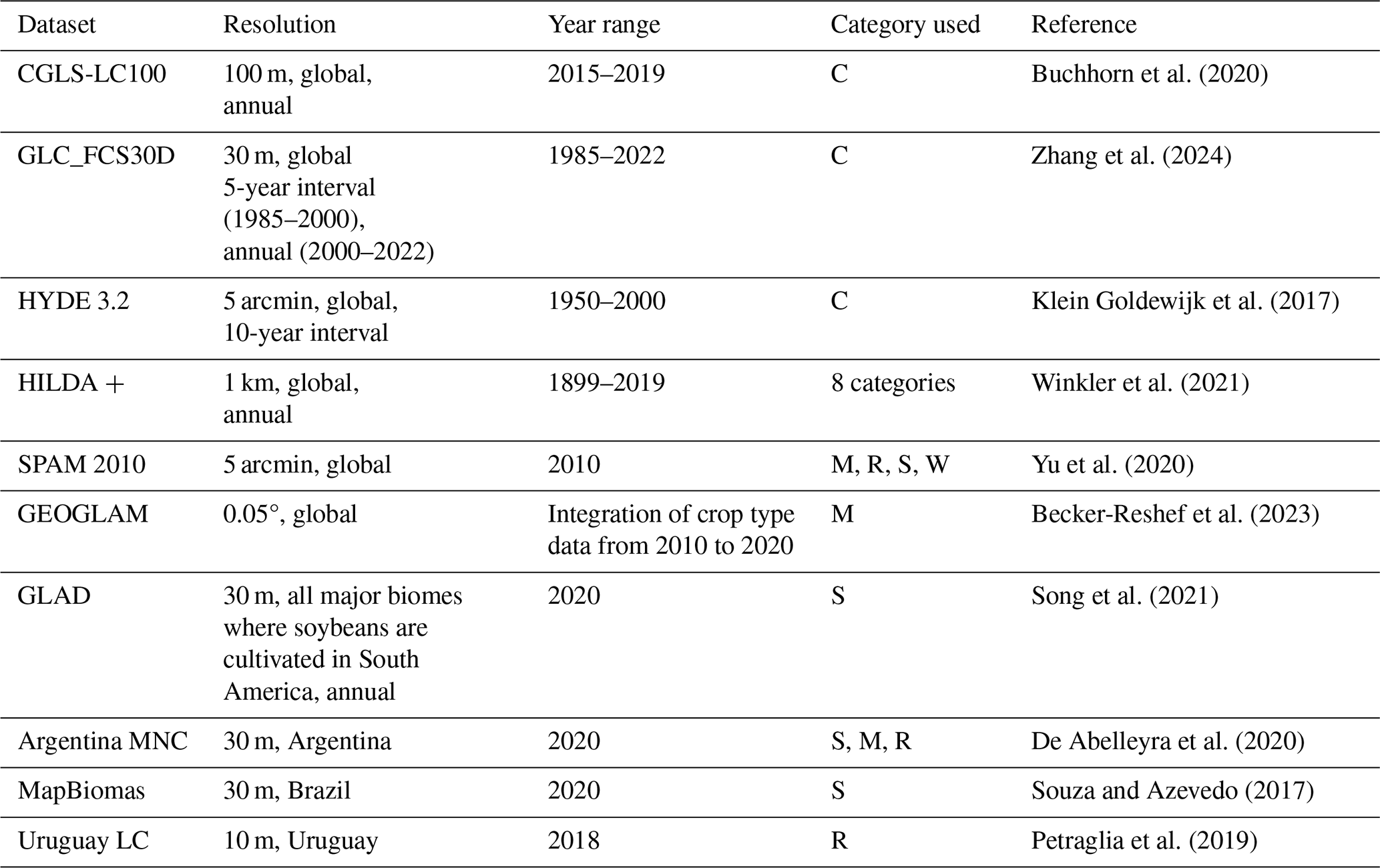
Copernicus Global Land Service Land Cover Map (CGLS-LC100). CGLS-LC100 is a newly developed global LULC dataset with 100 m spatial resolution from 2015 to 2019, containing 23 land use types (Buchhorn et al., 2020). This product uses PROBA-V 100 m time-series data and high-quality land cover training samples to construct a land cover classification model with 80 % accuracy at Level 1. It has been compared to other popular LULC products and proven to perform better, making it a good choice for generating a base map for cropland density maps (Tsendbazar et al., 2019).

Global 30 m Land Cover Dynamics Monitoring Dataset (GLC_FCS30D). GLC_FCS30D is a global land cover product with a 30 m resolution based on continuous change detection algorithms (Zhang et al., 2024). It uses a detailed classification system containing 35 land cover classes, covering the period from 1985 to 2022. The update cycle is 5 years before 2000 and annually after 2000. Moreover, it combines a continuous change detection algorithm, local adaptive classification models, and a spatial–temporal refinement method for dense time series to describe the land cover dynamics, verifying that the overall accuracy of the basic classification system for the 10 major land cover types exceeds 80 %.

The History Database of the Global Environment (HYDE version 3.2). HYDE 3.2 uses a spatial allocation algorithm to generate spatially explicit maps from 10 000 BCE to 2017 CE by integrating historical statistical data with recent satellite information (Klein Goldewijk et al., 2017). It includes cropland (irrigated and rainfed crops and irrigated and rainfed rice), grazing land (pasture and rangeland), and population maps with 5 arcmin spatial resolution. Numerous studies have demonstrated that HYDE 3.2 provides an excellent basis for reconstructing cropland density for historical periods (Li et al., 2023; Mao et al., 2023).

Historic Land Dynamics Assessment+ (HILDA+). HILDA+ is a comprehensive global dataset designed to track changes in land use and cover from 1899 to 2019 at a spatial resolution of 1 km (Winkler et al., 2021). This dataset is notable for integrating multiple datasets, including high-resolution remote sensing data, land use reconstructions, and long-term statistical records. HILDA+ captures the dynamics of various land use categories, such as urban areas, cropland, pasture/rangeland, forests, unmanaged grass/shrublands, and areas with sparse or no vegetation.

Spatial Production Allocation Model (SPAM 2010). SPAM 2010 integrates high-resolution remote sensing data and agricultural statistics to generate a comprehensive product of crop area, yield, and production (Yu et al., 2020). This dataset enhances previous models by including data for 42 major crops under four different farming systems across a global 5 arcmin grid. SPAM2010 addresses the limitations of administrative-level agricultural statistics by disaggregating them to a finer spatial resolution, thereby revealing the diversity and spatial patterns of agricultural production.

Group on Earth Observations Global Agriculture Monitoring (GEOGLAM). GEOGLAM is a global and up-to-date crop type map at 0.05° spatial resolution for four major commodity crops: wheat, maize, rice, and soybeans (Becker-Reshef et al., 2023). The development process involved extensive dataset selection and unification, considering factors such as seasonality, spatial resolution, accuracy, and data source specificity. These criteria ensure that the final maps are both accurate and useful for operational agricultural monitoring.

Global Land Analysis & Discovery (GLAD). GLAD provides soybean maps with a 30 m resolution for South America covering the period from 2000 to 2023 (Song et al., 2021). The products were derived by integrating all Landsat and MODIS images captured during the growth stage of soybeans. GLAD soybeans maps cover all major biomes in South America (i.e., Pampas, Chiquitania, Chaco, Cerrado, Atlantic Forest, Amazonia, and the Pantanal and Caatinga biomes). Validated using a probability sample of field observations across the continent, the GLAD soybean maps have an overall accuracy exceeding 94 % with both high user's and high producer's accuracy.

MapBiomas provides land use and land cover maps with a 30 m resolution for Argentina, Brazil, and Uruguay, which include the major land use and cover types, as well as some crop-specific information (e.g., soybean and rice). Argentina MNC provides detailed crop type maps (e.g., soybean, maize, and rice) with a 30 m resolution for Argentina from 2018 to 2022 (De Abelleyra et al., 2020). The data were generated by supervised classification of Landsat-8 observations using a random forest classifier to independently classify different agricultural zones, achieving an overall accuracy exceeding 80 % for both summer and winter crops. MapBiomas Brazil was generated using all available Landsat observations covering 1985 to 2022 and processed in Google Earth Engine, achieving an overall accuracy of around 80 % in most biomes at Level 1 (Souza and Azevedo, 2017). An integrated land cover/use map of Uruguay (Uruguay LC) was also generated in 10 m resolution with crop-specific information from 2018 (Petraglia et al., 2019).

To reconstruct the historical cropland and crop type dynamics, all datasets needed to be preprocessed. First, the high-resolution datasets (i.e., CGLS-LC100, GLC_FCS30D, GLAD, Argentina MNC, MapBiomas, and Uruguay LC) were aggregated to a 1 km resolution to attain the fractional cropland and crop type. Second, HYDE 3.2, SPAM 2010, and GEOGLAM were resampled to 1 km spatial resolution using the bilinear method. Finally, the projection of all datasets was transformed into WGS84 for further analysis, with all processes carried out in Google Earth Engine.

2.3.2 Inventory datasets

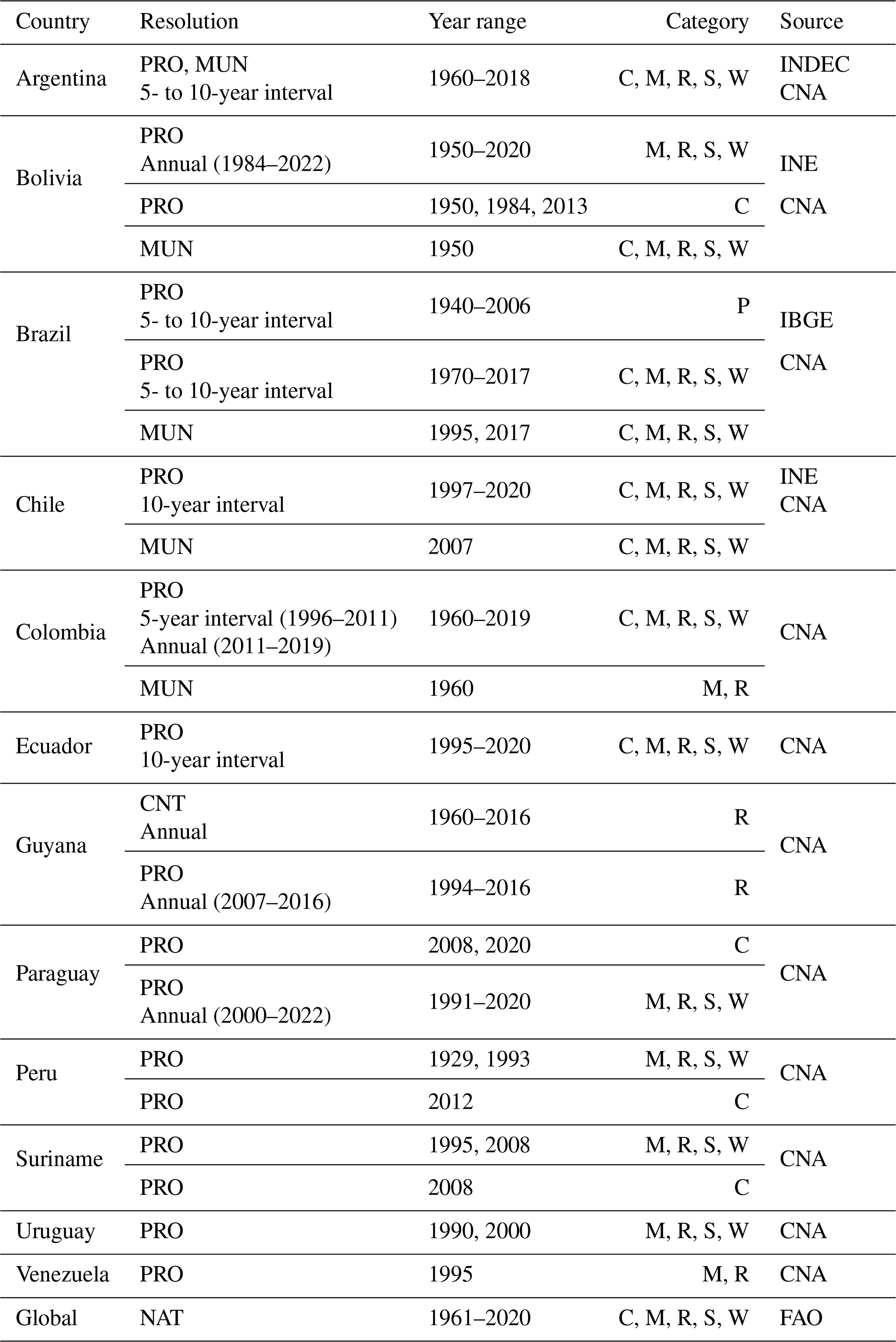
The inventory datasets were collected at three levels: national, provincial, and municipal. The national data mainly come from the Food and Agriculture Organization (FAO), while the provincial and municipal data primarily come from agriculture censuses released by governments (Table 2). Ultimately, a total of 136 provincial-level statistics on LULC and crop-specific information from 13 countries were collected and sorted to reconstruct historical crop-specific areas at the provincial level. Additionally, 10 municipal-level statistics were used to evaluate the crop-specific maps generated in this study.

Table 2 The inventory datasets used in this study. NAT: national; PRO: provincial; MUN: municipal; C: cropland; M: maize; R: rice; S: soybean; W: wheat; P: production. CNA: National Agricultural Census; INDEC, INE, IBGE, and INE are the national statistics and census bureaus of the corresponding countries. Due to the large number of data sources, detailed information is provided in Table S3.

2.4 Generating cropland density maps

We used both gridded and inventory datasets to generate cropland density maps at a resolution of 1 km × 1 km, covering the period from 1950 to 2020 (Fig. 2). All gridded datasets used in this section were first aggregated to a common spatial resolution of 1 km. All subsequent operations, including trend operation, interpolation, and cropland density adjustment, were performed at this resolution to ensure spatial consistency. Specifically, the reconstruction process consists of the following steps: (1) the reconstruction of a total cropland area at the provincial level covers the period from 1950 to 2020. In this step, we mainly used two complementary interpolation approaches: ratio-based interpolation and linear interpolation. For years with available national-level cropland area but missing provincial-level cropland area, we estimated provincial-level cropland area by scaling the nearest known provincial-level cropland area according to the relative change in national-level cropland area (Eq. 1). This assumes that provincial-level changes follow the same relative trend as those observed on the national scale. From 1961 to 2020, national cropland areas from FAO were used to calculate annual change rates. For years prior to 1961, we relied on agricultural census records or HYDE data. In cases where neither provincial nor national cropland areas were available, we applied linear interpolation between known provincial cropland areas. Since data availability and reference years differ across countries, the reconstruction was performed separately for each country. (2) Second, we generated the potential cropland density maps with a resolution of 1 km × 1 km from 1950 to 2020. Based on the definitions of various datasets and a comparison of total cropland area at the provincial level, we selected CGLS-LC100 (2015–2019), GLC FCS30D (1985–2022), and HYDE (1950–1990) as sources to generate potential cropland density maps (Tables S1 and S2 and Fig. S1 in the Supplement). Since CGLS-LC100 and the reconstructed cropland area exhibit high agreement at the provincial level (R²=0.92, RMSE = 0.46 Mha), we choose CGLS-LC100 as the baseline data for generating the potential cropland density maps. To extend cropland density maps prior to the availability of CGLS-LC100, we employed a backward projection method using GLC_FCS30D and HYDE. Specifically, we selected CGLS-LC100 in 2015 as the base map for GLC_FCS30D and 1990 as the base year for HYDE due to its decadal resolution. We then projected cropland density backward by applying annual or decadal fractional changes from these two datasets to their respective base maps. Accordingly, we applied the following rules to handle dataset integration.

• a.

  GLC_FCS30D > 0, CGLS_LC100 > 0: the relative change in cropland density between the years (e.g., 2014 to 2015 from GLC_FCS30D) was applied directly to the corresponding CGLS-LC100 grid cell.

• b.

  GLC_FCS30D > 0, CGLS-LC100 = 0: the product of any change rate and zero yields zero; thus, the cropland density for that year and grid cell remained zero.

• c.

  GLC_FCS30D = 0, CGLS-LC100 > 0: this implies no recorded change in cropland presence; thus, the CGLS-LC100 value was retained without adjustment.

A similar method was applied when using HYDE to reconstruct cropland density maps prior to 1985, with decadal change rates applied to the 1990 baseline. Since HYDE provides data at decadal intervals, we applied linear interpolation to fill in the annual gaps between 1950 and 1985 on a grid-by-grid basis. (3) Third, we adjusted the potential cropland density maps using reconstructed provincial-level cropland area to obtain an annual cropland density map between 1950 and 2020 (Eq. 2). If the cropland density of a grid is less than 0 or greater than 1, we assign it a value of 0 or 1, respectively. This adjustment process is repeated until the difference between the adjusted area and the total cropland area at the provincial level is less than 100 ha.

$$\begin{array}{}\text{(1)}& {\mathrm{CropArea}}_{c,s,i}={\mathrm{CropArea}}_{c,s,i+j}\times {\displaystyle \frac{\mathrm{Reference}{\mathrm{data}}_{c,i}}{\mathrm{Reference}{\mathrm{data}}_{c,i+j}}},\end{array}$$

where CropArea${}_{c,s,j}$ and CropArea${}_{c,s,i+j}$ are the reconstructed cropland area of province s in country c in year i and i+j and Reference data_c,i and Reference data${}_{c,i+j}$ are the reference values for the total cropland area in country c in year i and i+j, respectively. Between 1961 and 2020, the value of j is 1, while before 1961, the value of j corresponds to the year difference in the reference data.

$$\begin{array}{}\text{(2)}& {\mathrm{Grid}}_k^{\prime }={\mathrm{Grid}}_k+{\displaystyle \frac{\left(\mathrm{TotalArea}-\sum _{\mathrm{1}}^n{\mathrm{Grid}}_k\right)}{n}},\end{array}$$

where Grid${}_k^{\prime }$ is the adjusted cropland density for the kth grid, Grid_k is the potential cropland density, “TotalArea” is the reconstructed cropland area at the provincial level, and n is the total number of valid crop grids (cropland density > 0) in a province.

2.5 Generating gridded crop-specific maps

2.5.1 Building crop-specific base map for the year 2020

We set 2020 as the base year and generated the base map of four commodity crops (i.e., maize, rice, soybean, and wheat) by integrating multiple remote-sensing-based and model-based datasets. First, considering that high-resolution crop distribution maps do not cover the whole of South America, we used the resampled SPAM 2010 data to generate the initial base map. We then replaced the corresponding regions with higher-resolution data available for around 2020. Specifically, the base map for maize was generated from Argentina MNC (2020) and SPAM (2010). The base map for soybean was generated from Argentina MNC (2020), MapBiomas (2020), GLAD (2020), Uruguay LC (2018), Argentina MNC (2020), and SPAM (2010). The base map for wheat was generated from GEOGLAM (2020). Finally, we used reconstructed crop-specific harvested area in 2020 at the provincial level to further adjust the base map (Eq. 2).

2.5.2 Reconstructing the annual crop-specific harvested area at the provincial level

Long-term historical crop-specific harvested areas at the provincial level were reconstructed from 1950 to 2020 using multiple sources of historical inventory data (Table 2). The detailed reconstruction processes are described below. First, the time series of crop-specific harvested areas at the provincial level were obtained from the National Agricultural Census (CNA), the national statistics office (e.g., INDEC, IBGE, and INE, etc.), and the literature.

Second, anomaly values in the time series of crop-specific harvested area were identified and removed through visual inspection, based on the assumption that harvested area typically follows a gradual upward or downward trend over time. Years with abrupt deviations inconsistent with adjacent values were flagged as potential anomalies. Third, the FAO trend was used to fill the gaps between 1961 and 2020 (Eq. 1). Fourth, in countries where harvested area statistics were unavailable, crop-specific harvested areas were reconstructed using production data, based on the strong correlation between production and harvested area (R²=0.92, Eq. 3). Specifically, in Brazil from 1950 to 1970, provincial-level crop production data were used to estimate harvested areas, as no public statistics data were available during this period. For countries with no available data before 1961, we maintain consistency using the data from 1961. Finally, the liner interpolation was used to fill the crop-specific harvested area with the missing values.

$$\begin{array}{}\text{(3)}& {\mathrm{CTArea}}_{c,s,i}={\mathrm{CTArea}}_{c,s,i+j}\times {\displaystyle \frac{{\mathrm{Prod}}_{c,s,i}}{{\mathrm{Prod}}_{c,s,i+j}}},\end{array}$$

where CTArea${}_{c,s,j}$ and CTArea${}_{c,s,i+j}$ are the reconstructed crop-specific harvested area of province s in country c in year i and i+j and Prod${}_{c,s,i}$ and Prod${}_{c,s,i+j}$ are the crop production of province s in country c in year i and i+j.

2.5.3 Spatializing provincial-level data to generate annual crop-specific maps

The reconstructed crop-specific harvested area at the provincial level was spatially allocated to the grid level based on the generated crop-specific base map and annual cropland density to obtain 1 km crop-specific maps from 1950 to 2020. Specifically, we took 2020 as the baseline and used the ratio of cropland density between two adjacent years to obtain the density of the crop-specific harvested area in the previous year (Eq. 4). We assumed that the interannual trend in crop-specific harvested area is consistent with the trend in area changes in cropland density. To ensure that the allocated area is consistent with the total harvested area at the provincial level, we further adjusted the allocated crop-specific harvested area using Eq. (2).

$$\begin{array}{}\text{(4)}& {\mathrm{CTDensity}}_{k,i-\mathrm{1}}={\displaystyle \frac{{\mathrm{CropDensity}}_{k,i-\mathrm{1}}}{{\mathrm{CropDensity}}_{k,i}}}\times {\mathrm{CTDensity}}_{k,i},\end{array}$$

where CTDensity${}_{k,i-\mathrm{1}}$ and CTDensity_k,i are the density of crop-specific harvested area for the kth grid in years i and i−1 and CropDensity${}_{k,i-\mathrm{1}}$ and CropDensity_k,i are the cropland density for the kth grid in years i and i−1.

2.5.4 Analyzing crop-specific land use transitions

To assess the transitions between land use and specific crop types, we first converted the annual crop-specific density maps into Boolean crop type maps for each year from 1950 to 2020, following the method described by Li et al. (2023). For each crop and year, grid cells were ranked in descending order based on crop-specific density. Boolean values (presence = 1, absence = 0) were then assigned to the top-ranked grid cells until the cumulative area matched the reconstructed provincial-level harvested area within a 100 ha margin. This allocation was performed sequentially for soybean, maize, wheat, and rice, based on the availability and reliability of high-resolution crop-specific datasets. In particular, soybean and maize were prioritized because they are supported by well-validated spatial products (e.g., GLAD and Argentina MNC), which offer a reliable basis for anchoring the allocation and maintaining spatial consistency with observed crop distributions. To identify land use transitions associated with specific crops, we overlaid the annual Boolean crop type maps with the annual land use maps from the Historic Land Dynamics Assessment+ (HILDA+) (Winkler et al., 2021). This spatial overlay allowed us to determine which crop types occupied areas that had been newly converted cropland in a given year. It is important to note that this approach assumes that the spatial allocation based on crop-specific density rankings reflects the dominant crop type established after cropland conversion. While this process introduces some uncertainty, the method offers a consistent and spatially explicit framework for attributing land use change processes to specific crops in the absence of pixel-level crop rotation data.

2.6 Accuracy assessment

We performed accuracy assessments using three strategies: (1) we compared crop-specific areas derived from existing gridded products with those from this study at the provincial level. To ensure the reliability of the assessment, we used data from years not included as inputs, serving as an independent reference for the evaluation – i.e., MapBiomas (2000, 2005, and 2010), SPAM (2000 and 2005), GEOGLAM (2020), GLAD (2005 and 2010), and Brazil Conba (2017–2020, Table S3). (2) We validated reconstructed crop-specific maps in this study with crop-specific areas collected from agricultural censuses at the municipal level. (3) We performed visual comparisons using existing remote-sensing-based high-resolution data (Argentina MNC, GLAD, Uruguay LC, and WorldCereal) at the grid level. This process is primarily evaluated by calculating the difference between the fraction of our developed data and the fraction of other datasets within each grid. Given the limited availability of high-resolution data, we began by comparing data from around 2020 – i.e., Argentina MNC (2020), Uruguay LC (2018), and WorldCereal (2021). Additionally, GLAD data (2001, 2010, and 2020) were used for long-term series comparisons. For evaluation at the provincial and municipal levels, we used the coefficient of determination (R², Eq. 5), normalized root mean square error (nRMSE, Eq. 6), and slope (Eq. 7) to quantify the performance of our developed crop-specific data relative to other datasets. Higher R² values, lower nRMSE, and a slope closer to 1 indicate better agreement between actual and estimated crop-specific areas, and vice versa.

$$\begin{array}{}\text{(5)}& {\displaystyle }& {\displaystyle }{R}^{\mathrm{2}}=\mathrm{1}-{\displaystyle \frac{\sum _{i=\mathrm{1}}^n{\left(x_i-y_i\right)}^{\mathrm{2}}}{\sum _{i=\mathrm{1}}^n{\left(x_i-\stackrel{\mathrm{‾}}{x}\right)}^{\mathrm{2}}}},\text{(6)}& {\displaystyle }& {\displaystyle }\mathrm{nRMSE}={\displaystyle \frac{\sqrt{\frac{\mathrm{1}}{n}\sum _{i=\mathrm{1}}^n{\left(x_i-y_i\right)}^{\mathrm{2}}}}{\stackrel{\mathrm{‾}}{x}}},\text{(7)}& {\displaystyle }& {\displaystyle }\mathrm{slope}={\displaystyle \frac{\sum _{i=\mathrm{1}}^n\left(x_i-\stackrel{\mathrm{‾}}{x}\right)\left(y_i-\stackrel{\mathrm{‾}}{y}\right)}{\sum _{i=\mathrm{1}}^n{\left(x_i-\stackrel{\mathrm{‾}}{x}\right)}^{\mathrm{2}}}},\end{array}$$

where n represents the number of samples, x_i and y_i are the actual and estimated crop-specific areas for the ith sample, and $\stackrel{\mathrm{‾}}{x}$ and $\stackrel{\mathrm{‾}}{y}$ represent the average of the actual crop-specific areas.

3 Results

3.1 Dynamics of crop types from 1950 to 2020 in South America

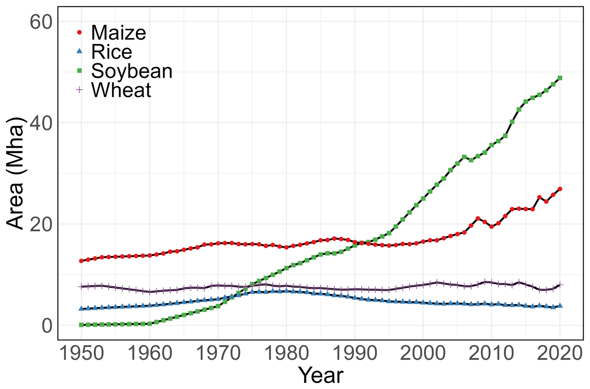
Figure 3 shows the spatial pattern of soybean, wheat, maize, and rice from 1950 to 2020 in South America. Overall, there has been a significant increase over time in the area and density of cultivation for all major crops. Soybean and maize have expanded significantly in Argentina and Brazil. Specifically, soybean was practically not cultivated in South America in 1950, with small amounts starting to appear in 1980. After 2000, soybean cultivation increased significantly, covering large areas in central and southern Brazil and central Argentina. Maize was initially cultivated mainly in central Argentina, southern Brazil, and northern Colombia and Venezuela. The extent and density of maize cultivation gradually increased, showing a trend of expansion from south to north. Rice is cultivated in a relatively small area in South America, mainly in Uruguay; in northern parts of Colombia and Venezuela; and in the Brazilian states of Maranhão, Tocantins, and Rio Grande do Sul. Except for an increase in the extent of cultivation around 1980, there has been relatively little change in the rest of the years. Wheat is more concentrated in southern South America, including the provinces of Buenos Aires, Córdoba, and Santa Fe in central Argentina; Rio Grande do Sul in southern Brazil; and Araucanía and Biobío in central Chile. Between 1950 and 2020, the extent of wheat cultivation remained relatively stable. Additionally, we calculated the changes in the total area of different crops in different countries and the whole of South America (Figs. 4 and S2). Soybean is the crop with the most rapid change in the area, growing from 0.08 Mha in 1950 to 48.8 Mha in 2020, a 610-fold increase. The area of maize showed a slow growth trend until 2000, increasing from 12.7 Mha in 1950 to 16.5 Mha in 2000. Since 2000, the growth rate has gradually increased, reaching a total area of 26.9 Mha in 2020, with an average annual growth rate of 6.8 times higher than that of the pre-2000 period. The area of rice increased gradually before 1980, growing from 3.2 Mha in 1950 to 6.7 Mha in 1980, followed by a gradual decline, falling back to 3.8 Mha by 2020. In contrast, wheat is relatively stable, increasing slightly from 7.6 Mha in 1950 to 7.9 Mha in 2020. At the country level, Brazil has the largest area of soybean, maize, and rice, while Argentina has the largest area of wheat. These trends reflect the significant agricultural transformations in South America. The rapid growth in soybean and maize cultivation is especially notable, aligning with global shifts in commodity markets, while rice and wheat have shown more moderate changes over time.

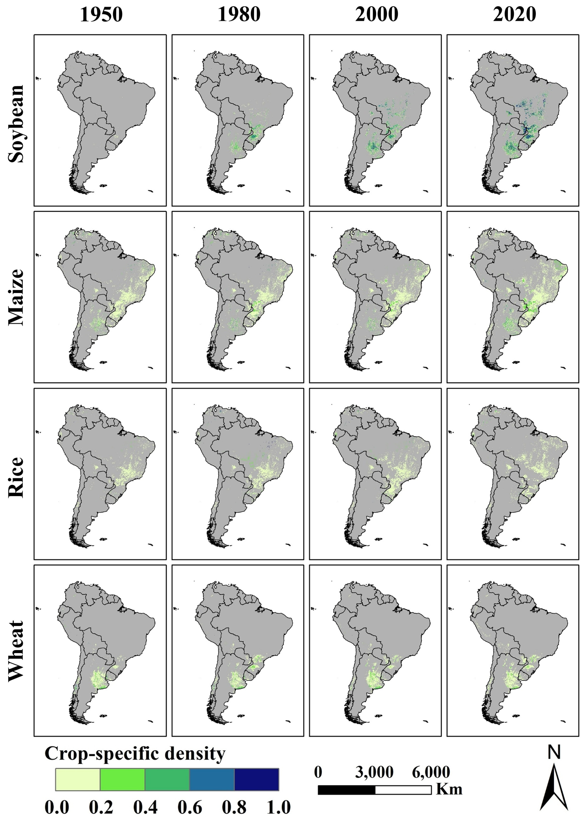
Figure 3 The spatial pattern of soybean, maize, rice, and wheat from 1950 to 2020. The first, second, third, and fourth rows represent the crop-specific fraction of soybean, maize, rice, and wheat. Crop-specific density represents the proportion of a given crop within each 1×1 km grid.

Figure 4 Temporal changes in crop-specific areas in South America during 1950–2020.

3.2 Crop-specific land use transitions

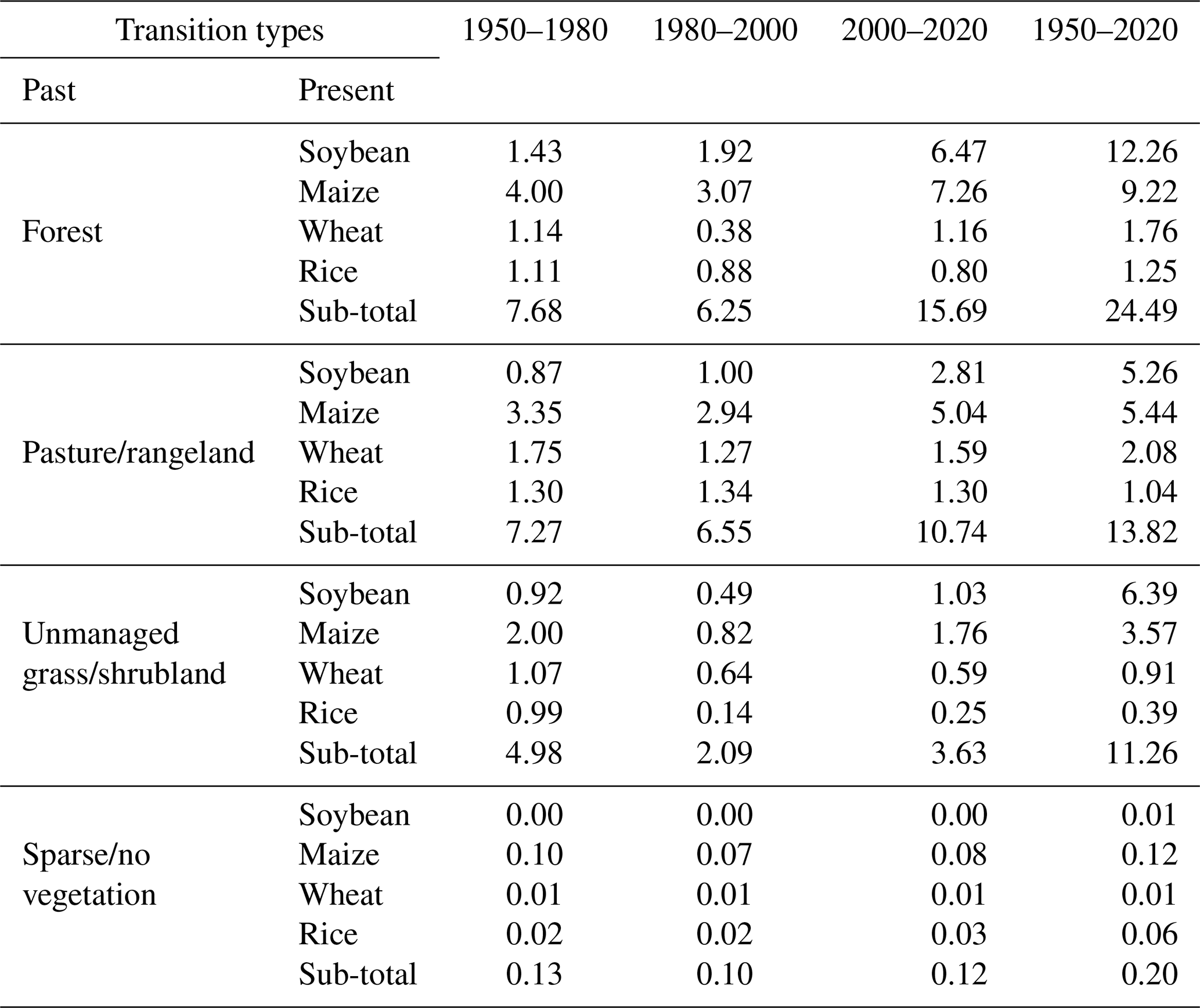
Over the past 70 years, soybean and maize have expanded dramatically through encroachment on other vegetation, including forest, pasture/rangeland, and unmanaged grass/shrubland (Fig. 5 and Table 3). Specifically, 24.49 Mha of the forest was converted into the four major crops. Additionally, 13.82 Mha of pasture/rangeland, 11.26 Mha of unmanaged grass/shrubland, and 0.20 Mha of sparse/no vegetation were also converted. Most of this conversion was into soybean, accounting for 23.92 Mha, which represents 48.1 % of the total converted area. Regarding crops, different types exhibit varying extents of spatial expansion and encroachment on other vegetation. The total area of soybean encroaching upon forest, pasture/rangeland, and unmanaged grass/shrubland was 12.26, 5.26, and 6.39 Mha, respectively. The growth rate of encroachment upon forests increased rapidly from 0.05 Mha yr⁻¹ in 1950–1980 to 0.32 Mha yr⁻¹ in 2000–2020. In terms of spatial distribution, soybean encroachment occurred mainly in the Brazilian provinces of Mato Grosso, Paraná, and Rio Grande do Sul, as well as in southeastern Paraguay and central Bolivia for forests; in eastern Argentina and parts of Brazil for pasture/rangeland; and at the confluence of the provinces of Maranhão, Piauí, and Bahia for grasslands. On the other hand, the total area of maize encroachment from forest, pasture/rangeland, and unmanaged grass/shrubland was 9.22, 5.44, and 3.57 Mha, respectively. The growth rate of encroachment from forests increased from 0.13 Mha yr⁻¹ in 1950–1980 to 0.36 Mha yr⁻¹ in 2000–2020. The spatial pattern of maize encroachment was similar to that of soybean. The expansions of other crops are smaller in area compared to soybeans and maize and more dispersed in their spatial distribution. Overall, cropland expansion led to significant reductions in other vegetation, with the most dramatic increase occurring in staple crops, particularly soybean and maize.

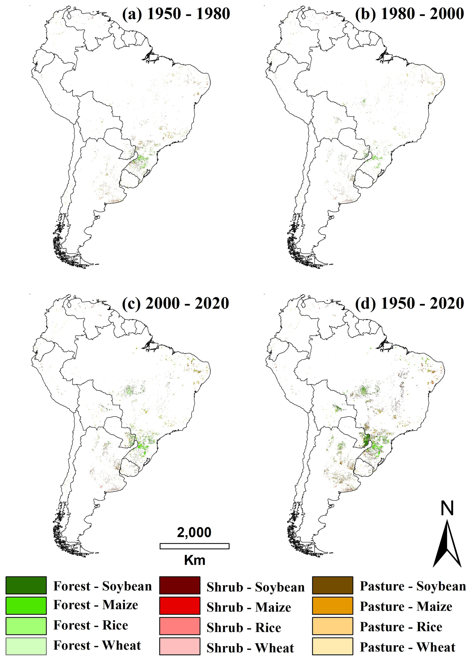
Figure 5 Spatial pattern of transitions between LULC and crop-specific areas from 1950 to 2020. (a) 1950–1980; (b) 1980–2000; (c) 2000–2020; (d) 1950–2020. Pasture: pasture/rangeland. Shrub: unmanaged grass/shrubland.

Table 3 Statistics of transition areas in South America from 1950 to 2020 (unit: Mha).

3.3 Evaluation of the crop-specific maps

3.3.1 Evaluation against existing datasets at the provincial level

We compared the crop-specific areas (i.e., soybean, wheat, maize, and rice) derived from existing datasets with the crop-specific maps developed in this study at the provincial level (Fig. 6). We used gridded datasets that were not involved in the base map generation to ensure independence from the reconstruction process, including MapBiomas (soybean and rice in 2000, 2005, and 2010), SPAM (soybean, wheat, maize, and rice in 2000 and 2005), GEOGLAM (soybean, maize, and rice), GLAD (soybean in 2005 and 2010), and Brazil Conab (soybean and rice from 2017 to 2020). The soybean areas from this study are consistent with Brazil Conab (Fig. 6a: R²=1, slope = 1.38) and SPAM (R²=0.96, slope = 1.15) but lower than those from MapBiomas (R²=0.99, slope = 1.41), GEOGLAM (R²=0.92, slope = 1.49), and GLAD (R²=0.91, slope = 1.56). The wheat areas from this study are consistent with SPAM (Fig. 6b: R²=0.93, slope = 1.15). The maize areas from this study are generally consistent with SPAM (Fig. 6c: R²=0.94, slope = 1.01). However, they differ significantly from those of GEOGLAM (R²=0.65, slope = 3.36). For rice, the areas from this study match well with Brazil Conba (Fig. 6d: R²=1, slope = 1.93) and SPAM (R²=0.87, slope = 1.15) but differ significantly from those of GEOGLAM (R²=0.70, slope = 0.83) and MapBiomas (R²=0.66, slope = 0.55). Generally, the crop-specific areas reconstructed in this study were consistent with other datasets, with most R² values exceeding 0.87, except for maize and rice in GEOGLAM and wheat in MapBiomas. This suggests that our method is reliable in reconstructing crop-specific areas at the provincial level despite some discrepancies. These discrepancies may be attributed to variations in data sources, processing methods, or classification criteria.

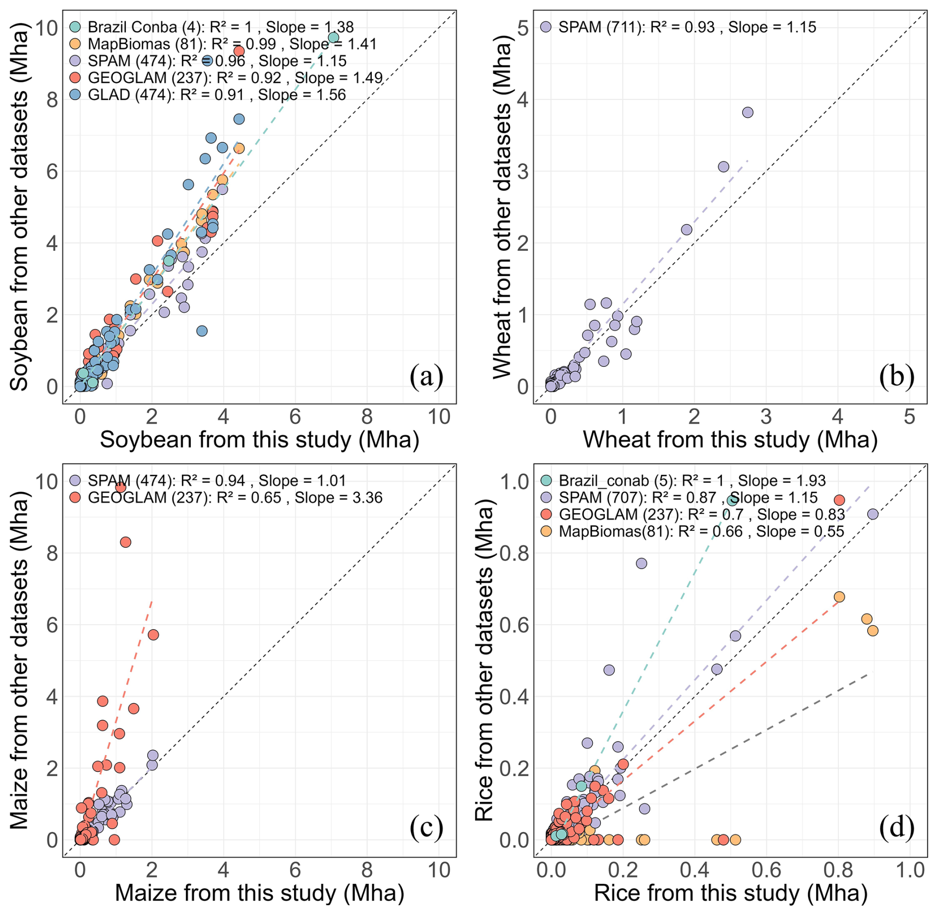
Figure 6 Comparison of crop type areas between this study and existing datasets (gridded datasets that were not involved in reconstruction process, i.e., Brazil Conba (2017–2020), MapBiomas (2000, 2005, 2010), SPAM (2000, 2005), GEOGLAM (2020), GLAD (2005, 2010)) at the provincial level. (a) Soybean; (b) wheat; (c) maize; (d) rice. The numbers in parentheses represent the total number of samples.

3.3.2 Evaluation using inventory data at the municipal level

To ensure the effectiveness of the evaluation, we collected crop type areas from various countries across different years at the municipal level to evaluate our reconstructed crop type maps (Argentina: 1960, 2008, and 2018; Bolivia: 1950; Brazil: 1995, 2006, 2017; Chile: 2017; Colombia: 1960; Paraguay: 2008). Figure 7 shows the comparison results of crop-specific areas for soybean, wheat, maize, and rice at the municipal level between census data and this study. We used R² and nRMSE to quantify the precision and reliability of our data. Specifically, the soybean and wheat areas derived from this study fit well with those from census data (soybean: R²=0.93, nRMSE = 0.0106; wheat: R²=0.79, nRMSE = 0.0151), whereas the performance of the maize and rice is less accurate (maize: R²=0.65, nRMSE = 0.0143; rice: R²=0.61, nRMSE = 0.0184). Additionally, the spatial pattern of soybean, maize, wheat, and rice proportions (i.e., crop-specific area/municipal area) is consistent with the census data (Figs. 8 and S3–S5). Soybean cultivation in Brazil is concentrated in the southern and central regions, and the soybean proportions derived from this study are relatively close to the census data, with minor over- and underestimates in only a few areas, such as Paraná and Rio Grande do Sul. On the other hand, Argentina shows a similar geographical distribution pattern, with the main cultivation areas concentrated in the central region but with overestimation in some areas. The main concentration is in the provinces of Córdoba and Buenos Aires. The areas for the remaining three crops (i.e., maize, wheat, and rice) are in good agreement with the census data, except for Brazilian maize in 2017, which is slightly underestimated in central Brazil.

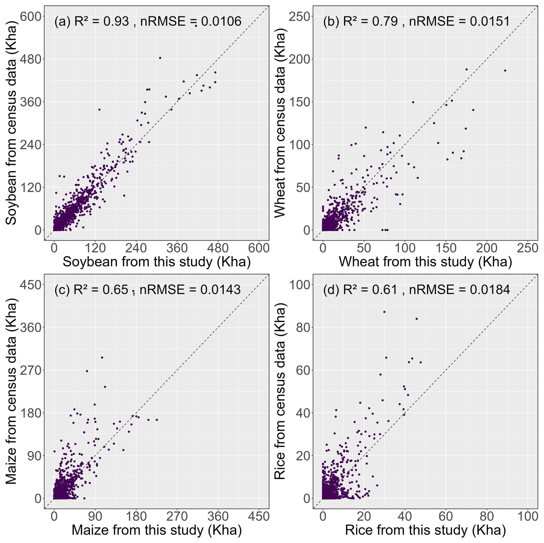
Figure 7 Comparison of the crop-specific areas between this study and census data at the municipal level. (a) Soybean; (b) wheat; (c) maize; (d) rice. The municipal-level inventory data used include Argentina (1960, 2008, and 2018), Bolivia (1950), Brazil (1995, 2006, and 2017), Chile (2017), Colombia (1960), and Paraguay (2008).

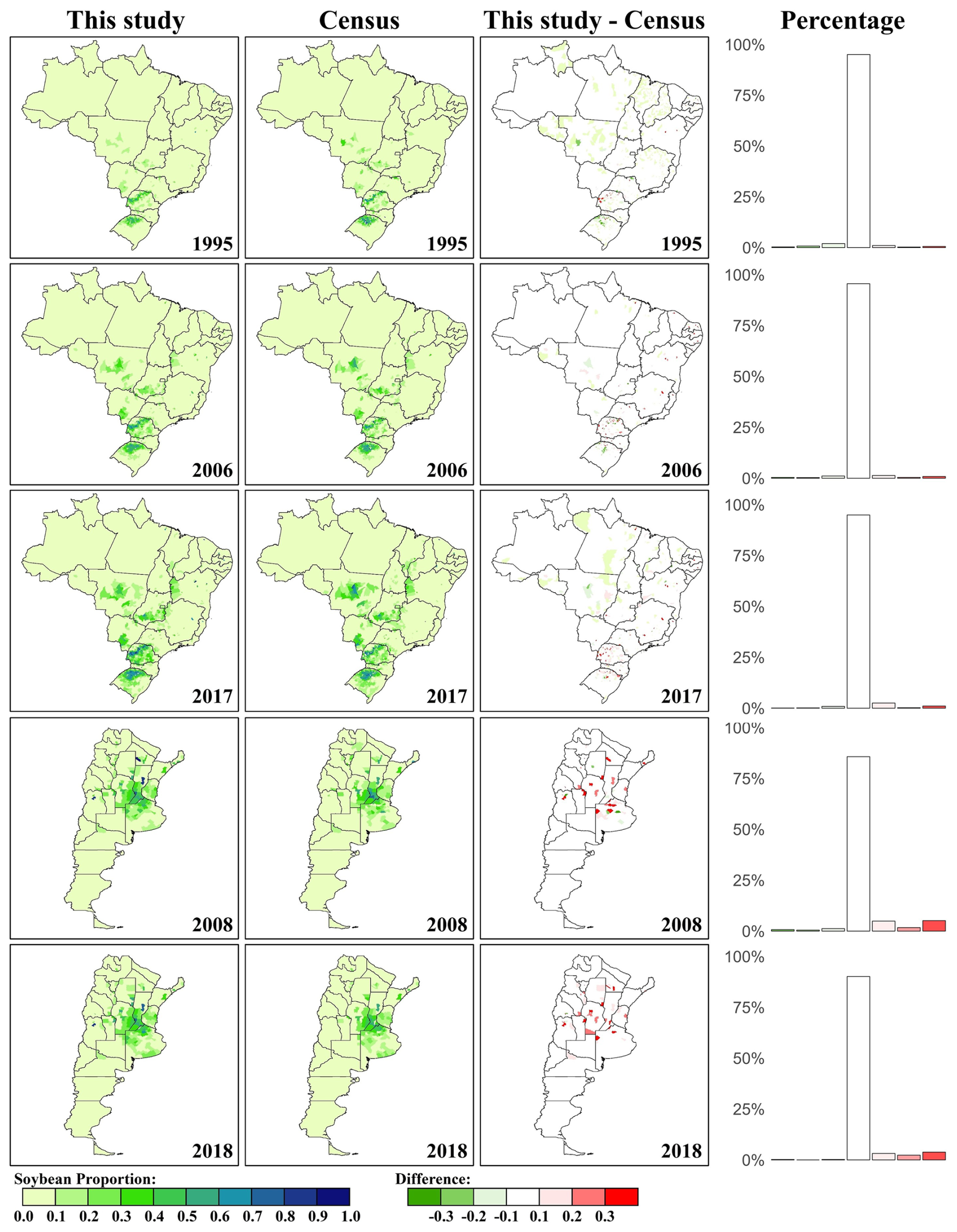
Figure 8 Spatial comparison of the soybean proportion (i.e., soybean area/municipal area) between this study and census data at the municipal level in Argentina (2008 and 2018) and Brazil (1995, 2006, and 2017). Proportions were calculated by aggregating gridded crop type data (allocated from provincial level statistics) and dividing by municipal area. These were compared with official municipal statistics processed in the same way. Left column: soybean proportion from this study; middle column: soybean proportion from census data; right column: the difference in soybean proportion between this study and census data.

3.3.3 Evaluation using satellite-based datasets at the grid level

We also compared satellite-based crop type maps with our reconstructed data at the grid level. Due to the lack of crop type maps for the whole of South America, we used Argentina MNC and Uruguay LC as baselines for the comparison of soybean, wheat, and maize. However, some maps generated by satellite data do not distinguish wheat from winter cereals (Van Tricht et al., 2023), so we used the resampled GEOGLAM as the baseline for the comparison of wheat. Figure 9 shows the spatial comparison of soybean, wheat, maize, and rice between satellite-based data and reconstructed data at the grid level. The results of the estimation of the proportion of soybean, wheat, maize, and rice cultivation show high agreement with the satellite data in terms of spatial distribution. However, there were slight over- or underestimates in some areas, especially in regions with concentrated crop cultivation. The percentage histograms provide detailed information on the distribution of differences, with most of the differences being less than 10 %, indicating that the estimation results of this study are generally reliable. Since most satellite-based crop maps are from around 2020 and are used as base maps to reconstruct historical crop distributions, we used soybean time-series data from GLAD to further assess the reliability of our reconstructed data. We chose 2001, 2010, and 2020 for comparison, with only the 2020 data used to construct the base map in Sect. 2.5.1. As shown in Fig. 10, the estimates from this study also show high agreement with the GLAD data in terms of spatial distribution for 2001, 2010, and 2020, with differences of less than 10 %.

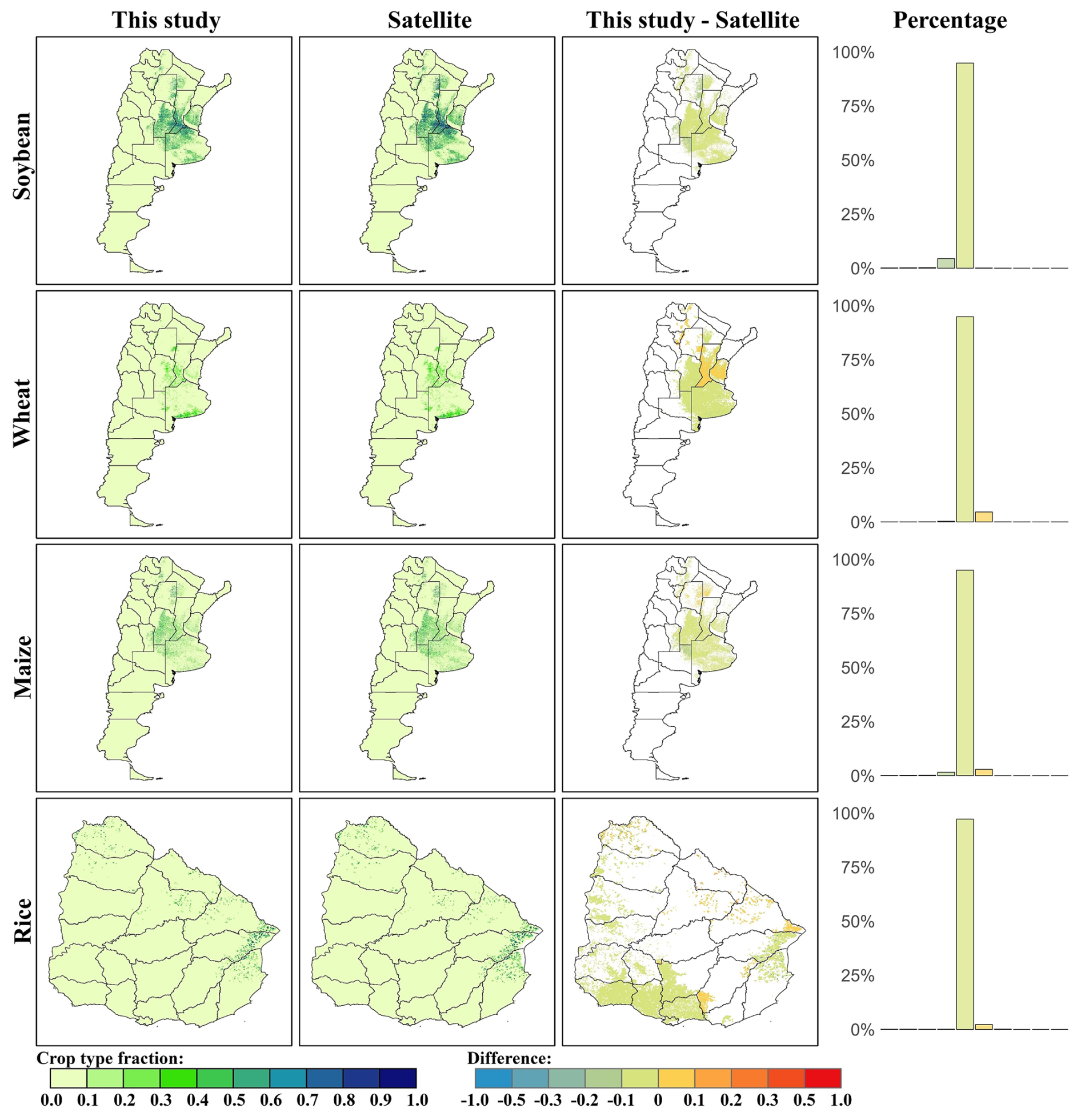
Figure 9 Spatial comparison of soybean, wheat, maize, and rice maps between satellite-based high-resolution data and the reconstructed data from this study. The soybean and maize maps are from Argentina MNC, the rice map is from Uruguay LC, and the wheat map is from GEOGLAM due to the lack of high-resolution data.

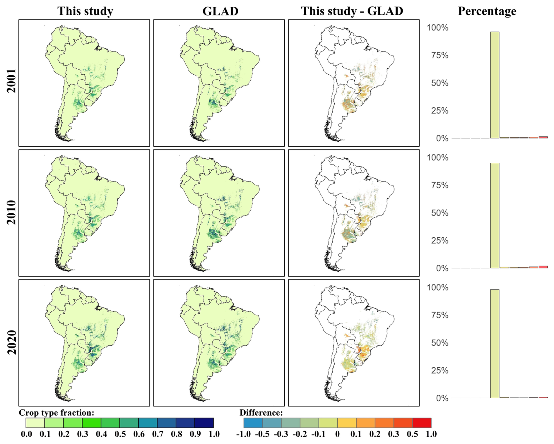
Figure 10 Spatial comparison of soybean maps between satellite-based high-resolution data (i.e., GLAD soybean) and the reconstructed data from this study for the years 2001, 2010, and 2020.

4 Discussion

4.1 Comparison with other datasets

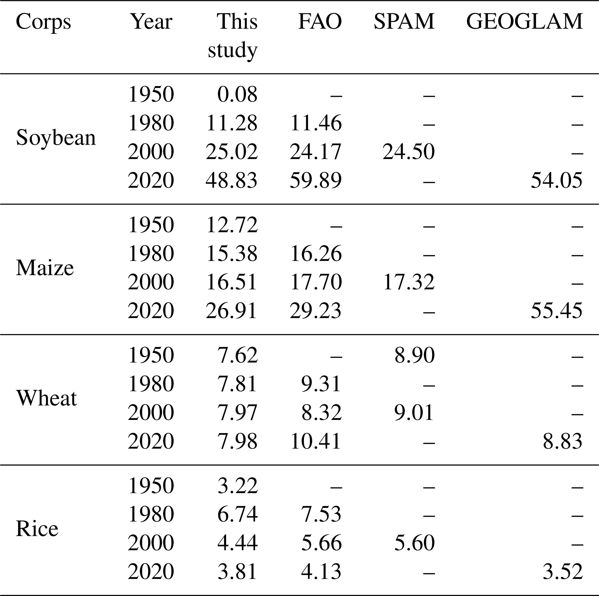
We first compared the area changes of four main crops (maize, rice, soybean, and wheat) in South America from 1950 to 2020 using FAO, GEOGLAM, GLAD, SPAM, and our reconstructed data (Table 4). Before 2000, the soybean area reconstructed in this study was highly consistent with FAO data, but after 2000, the reconstructed soybean area was lower. This discrepancy mainly originates from countries with larger soybean areas, such as Argentina and Brazil (Fig. S6). The census data we used were collected from the national statistical offices and the agricultural census inventory. In contrast, FAO data are mainly provided by member countries, making it challenging to ensure data accuracy (FAOSTAT). Additionally, Song et al. (2021) reported that the soybean area in the major biomes of South America increased from 26.4 Mha in 2001 to 55.1 Mha in 2019, which is comparable to the data reconstructed in this study and shows greater consistency at the country level. It is worth noting that SPAM also used provincial-level data for modeling, but the total soybean area is consistent with FAO and higher than that in this study. This is because SPAM corrected the allocation results using FAO national-level data, whereas our results were corrected based on provincial-level statistics (Yu et al., 2020). On the other hand, the soybean area in GEOGLAM is much higher than in other datasets. This difference arises because GEOGLAM integrates crop-specific maps at global and regional scales, spanning a wide range of periods (Becker-Reshef et al., 2023). For the remaining three crops (i.e., maize, wheat, and rice), our reconstructed data and other datasets showed high agreement across South America. However, the area of maize derived from GEOGLAM data is much higher than the others, for the reasons discussed above. Therefore, due to the lack of high-resolution data for wheat and relatively stable wheat area after 2010, we used only the GEOGLAM wheat distribution map as a base map. Additionally, the comparison with multiple reference datasets shows that slope values between our reconstructed cropland area at the provincial level vary across sources (Fig. 6). When compared to SPAM – a dataset that also incorporates official statistics – the slope values are largely within the range of 0.90 to 1.21 across crop types, indicating strong agreement and suggesting that our product is reliable in representing provincial-scale cropland distribution. In contrast, comparisons with remote-sensing-based datasets exhibit larger deviations. These discrepancies are expected due to differences in data sources and classification uncertainties. Overall, our reconstructed data are in good agreement with other existing datasets and utilize finer-grained statistics to generate spatially explicit crop type distribution maps.

Table 4 Comparison of crop-specific areas with other datasets in South America from 1950 to 2020 (unit: Mha).

Additionally, we performed a comparison of the distribution of different crop types at both spatial and temporal scales (Figs. 11 and 12). Specifically, the spatial distribution of soybean, maize, and rice is highly consistent with the high-resolution crop-specific distribution maps derived from remote sensing imagery and has a higher spatial resolution compared to GEOGLAM, providing more detailed information on crop-specific cultivation patterns. Due to the lack of high-resolution wheat distribution maps, we used WorldCereal as a potential wheat distribution map for comparison. WorldCereal is a winter cereal map that includes wheat, barley, and rye (Van Tricht et al., 2023). Although Fig. 11 demonstrates strong spatial agreement between our reconstructed data and existing high-resolution crop maps for 2020, some of these maps were also used to construct the base map, which may partially account for the high levels of consistency. To further evaluate the temporal reliability of our dataset, GLAD, being the only soybean distribution maps in South America with a high-resolution and long-duration time series and validation accuracy, allows us to compare spatial distributions of reconstructed data over time (Song et al., 2021). As shown in Fig. 12, we selected the Brazilian state of Mato Grosso, one of the most significant regions for soybean expansion since 2000, as an example to present comparative results. GLAD maps show clear signals of frontier expansion, while our results emphasize more gradual intensification. This difference may be attributed to the fact that our reconstruction is based on harmonized census data and historical cropland density, which may limit its ability to capture abrupt shifts as precisely as the high-resolution satellite-based maps. Nevertheless, our results remain broadly consistent with high-resolution products in terms of spatial patterns. Importantly, our dataset provides long-term, annually resolved crop-specific maps from 1950 to 2020, filling key temporal gaps that satellite-only datasets cannot address. Thus, despite limitations in detecting fine-scale expansion, the HISLAND-SA (HIStory of LAND transformation by humans in South America) dataset complements existing remote-sensing products by offering a coherent and historically extended view of crop type dynamics in South America.

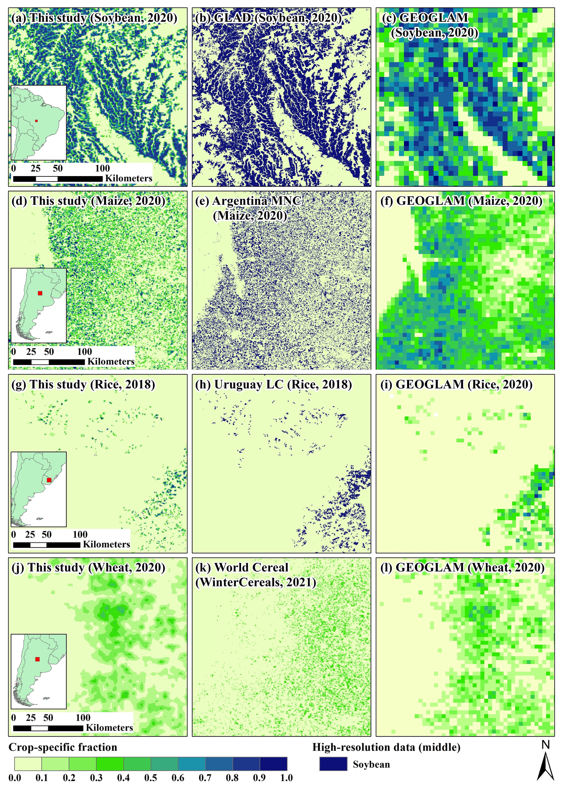
Figure 11 Visual comparison of crop-specific maps between this study and other datasets. The left column (a, d, g, j) shows the crop-specific maps in this study, with high-resolution data in (b), (e), (h), and (k) and coarse-resolution data in (c), (f), (i), and (l). Panels (b), (e), (h), and (l) were also used as input layers in generating the 2020 base map.

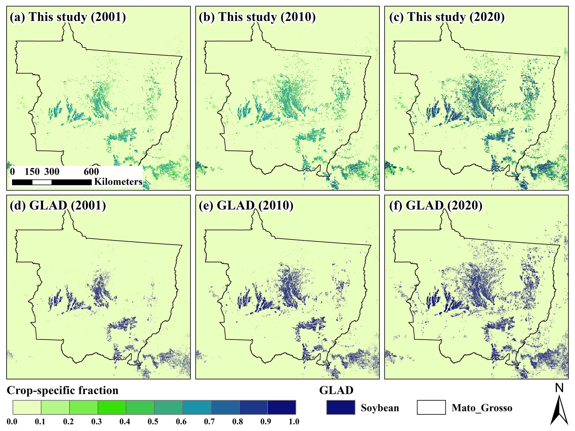
Figure 12 Temporal visual comparison of soybean fraction with GLAD.

4.2 Drivers of crop type changes

Agricultural expansion has led to dramatic land use changes in South America over the past few decades (Potapov et al., 2022; Winkler et al., 2021). In this study, we reconstructed crop-specific maps for South America over the past 70 years by integrating agricultural census data, model-based data, and remote-sensing-based crop type data and quantified the land use transitions caused by agricultural expansion. Our results show that the soybean area in South America increased from nearly zero in 1950 to 48.8 Mha in 2020. In South America, soybeans were initially cultivated on small farms primarily to provide animal feed and serve as a rotation crop adjunct to wheat (Klein and Luna, 2021). By the 1970s, the soybean industry began to emerge, driven by the surge in global protein meal prices (Richards et al., 2012; Warnken, 1999), new geopolitical alliances, and grain–livestock–fuel dynamics (de LT Oliveira, 2017). Simultaneously, the Brazilian National Agricultural Research Centre of Brazil (i.e., Embrapa) developed new soybean varieties adapted to the tropical climate and successfully introduced them into the Cerrado region in the Brazilian Midwest, which contributed to the “tropicalization of the soybean” and significantly expanded the soybean cultivation area (Klein and Luna, 2021). Driven by market-oriented reforms, globalization, and advancements in technology, the total soybean exports have burgeoned, further leading to a surge in soybean acreage (da Silva et al., 2021; Song et al., 2021). However, such a dramatic expansion in the soybean area is bound to have far-reaching consequences for land use change in South America. Over the past 70 years, soybean expansion has led to the loss of nearly 23.92 Mha of other vegetation, with forest accounting for 12.26 Mha, pasture/rangeland for 5.26 Mha, and unmanaged grass/shrubland for 6.39 Mha (Table 3). This extensive land use change has led to several environmental problems, including biodiversity loss, carbon emissions, land degradation, and water pollution (Baumann et al., 2017; Fearnside, 2002; Fehlenberg et al., 2017; Pengue, 2005; Song et al., 2021). Additionally, maize expansion is also one of the primary factors contributing to land use change and environmental threats in South America. Until the 1990s, changes in maize area were relatively stable and concentrated in traditional agricultural regions (e.g., the Pampas region in Argentina and the southern region in Brazil), primarily for domestic consumption as a major source of food for humans and livestock (Warnken, 1999). After the year 2000, maize cultivation in South America witnessed rapid growth, with maize being widely used not only as a food crop but also for biofuel production (Costantini and Bacenetti, 2021). During this period, maize acreage and yield increased significantly, with Brazil and Argentina becoming two of the world's leading producers and exporters of maize (Klein and Luna, 2022). By 2020, the maize area in South America had increased by a factor of 2.1 compared to 1950, encroaching on a total of 18.35 Mha of other vegetation, including 9.22 Mha of forests, 5.44 Mha of pasture/rangeland, and 3.57 Mha of unmanaged grass/shrubland (Table 3). Despite the importance of soybean and maize in the agricultural expansion of South America, wheat and rice have maintained their position as the main food crops. The expansion of soybean and maize cultivation has largely encroached on non-traditional farmland, such as forest and pasture, while wheat- and rice-growing areas have changed less. For wheat and rice, the change in area has remained relatively stable over the past 70 years, generally staying between 5 and 10 Mha. Wheat and rice are grown in relatively stable areas to ensure food security, even though other crops may offer higher economic returns (Jat et al., 2016). Additionally, several governments in South America have traditionally provided sustained policy support for wheat and rice cultivation, encouraging farmers to maintain a certain level of cultivation to ensure a stable food supply (Altieri, 1992; Warnken, 1999). The more recent notable expansions in South America invite attention to be given to the broader economic and legal changes that have facilitated or incentivized these drastic farming and agriculture changes, including through capital, finance, trade, and investment dynamics (Pistor, 2019; Saab, 2018).

4.3 Uncertainty analysis

4.3.1 Spatial and temporal gaps in census data

A key consideration in reconstructing historical land use dynamics is the availability of agricultural census data. Ideally, sub-national level (e.g., municipality, county, or district) agricultural statistics would allow for more detailed spatial allocation of crop-specific harvested areas. However, their availability across South America is highly limited and temporally inconsistent. Most countries provide only a few isolated years of data at the municipal level (i.e., Argentina: 1960, 2008, 2018; Bolivia: 1950; Brazil: 1995, 2006, 2017; Chile: 1960; Paraguay: 2008), which creates large temporal gaps and hampers their direct use in annual time-series reconstruction. In contrast, provincial level data are more consistently reported over time, typically at 10-year intervals. These more frequent observations enable more robust interpolation and better constrain the temporal evolution of harvested area. While these provincial units represent a coarser administrative granularity, we combined them with a high-resolution crop-specific base map and temporal cropland density maps to spatially disaggregate the data across all years. This approach allows us to preserve long-term trends while capturing spatial variability. To address the temporal discontinuities between census years, we applied linear interpolation to construct continuous annual times series of harvested areas at the administrative level. While we acknowledge that the use of linear interpolation may not fully reflect potential non-linear trends driven by policy, market, or environmental drivers, it remains a practical and widely used method under the constraints of sparse historical data (Klein Goldewijk et al., 2017; Leite et al., 2011; Li et al., 2023; Liu and Tian, 2010; Ye et al., 2024). Additionally, linear interpolation in this study is always bounded by observed census points, which help to preserve long-term trends and prevent fluctuations.

4.3.2 Resampling-related spatial uncertainty

To ensure spatial consistency across input datasets, we employed two resampling strategies to achieve a standardized 1 km resolution: (1) aggregation of high-resolution remote sensing products and (2) upsampling of lower-resolution datasets, such as SPAM. While resampling is essential for harmonizing spatial scales, it introduces varying degrees of uncertainty depending on the original resolution and classification accuracy of the source data.

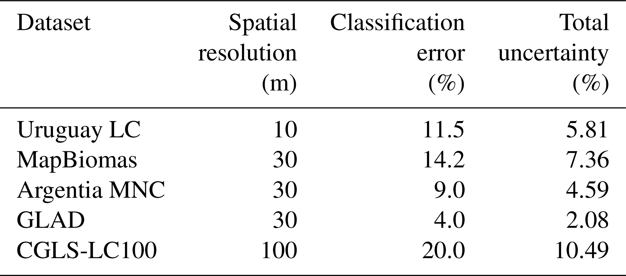
Aggregation of high-resolution datasets does not introduce additional spatial uncertainty beyond the inherent classification errors present in the original data. However, these classification errors can propagate into aggregated outputs and finally affect spatial statistics. To quantify this aggregation-induced uncertainty, we conducted a Monte Carlo simulation by introducing symmetric random noise at various classification error rates (i.e., 3 % to 15 %), whereby a proportion of target and non-target pixels were randomly flipped. For each combination of classification error rate and true fraction, we aggregated the modified raster to 1 km resolution and calculated the resulting aggregated fraction. This process was repeated 100 times per fraction to obtain stable estimates of the mean and standard deviation of the aggregated values (Fig. S7). We then computed the uncertainty as a function of both classification error and spatial resolution. Specifically, total uncertainty was defined as the average absolute deviation between aggregated and true values across the full range of possible true fractions (i.e., 0 % to 100 %). This allowed us to isolate the magnitude of uncertainty attributable to aggregation process. This simulation framework was applied to each of the aggregation datasets, yielding the acceptable uncertainties (Table 5). These results demonstrated that total uncertainty increases with both classification error and coarser input resolution. Datasets with higher native resolution (e.g., Uruguay LC) tend to exhibit lower aggregation uncertainty, even when classification error is moderate. This underscores that aggregation-induced uncertainty is a function not solely of accuracy, but also of the granularity of the input data. This uncertainty component must be explicitly considered when integrating heterogeneous land cover datasets for spatial modeling or policy-relevant assessments.

Table 5 Aggregation-induced uncertainty under varying classification errors and spatial resolutions.

To evaluate the spatial uncertainty introduced by the upsampling process, we conducted a quantitative comparison between SPAM and GLAD soybean maps for 2010 in South America. The original SPAM data were upsampled to 1 km using bilinear interpolation, while the GLAD soybean layer was aggregated to 1 km resolution and treated as reference. A pixel-by-pixel comparison was performed between the two datasets across the continent. First, the pixel-wise comparison yielded a coefficient of determination (R²) of 0.50, indicating moderate agreement between resampled SPAM and GLAD data. Second, the distribution and frequency of pixel-level differences revealed that over 70 % of the pixels fell within a ±0.1 range, while larger deviations (greater than ±0.3) were mainly observed in fragmented and heterogeneous cropping regions (Fig. S8). Although the resampling process introduced local structure uncertainty and smoothed fine-scale heterogeneity, these results suggest that the unsampled 1 km SPAM data retain meaningful broad-scale spatial patterns. Therefore, the resampled dataset in this study remains suitable for use as a baseline crop distribution map at continental scale.

4.3.3 Spatial–temporal consistency assessment

To assess the spatial and temporal consistency of our reconstructed crop type maps, we conducted an uncertainty analysis using the resampled GLAD 1 km soybean density dataset from 2001 to 2020 as an independent benchmark. This analysis focuses on evaluating whether the interannual variation in soybean density reflects actual crop dynamics. Figure 13 illustrates the annual difference in soybean density at the pixel level across South America. The results show that the median and mean differences remain close to zero over time, with narrow interquartile ranges (25 %–75 %) and relatively stable 5 %–95 % quantile envelopes. These findings suggest that the year-to-year fluctuations in our dataset are not random but follow a consistent trend with GLAD data, indicating reliable temporal comparability. In addition, Fig. S9 presents the spatial distribution of the mean soybean density difference averaged over the 20-year period, along with a histogram of its pixel-wise distribution. Most regions exhibit minimal bias, with more than 50 % of grids falling within ±0.1. The distribution is systematically centered around zero, and areas of substantial over- or underestimation are spatially limited. These two evaluations together evidence that our data maintain robust agreement with independent observations (i.e., GLAD) both spatially and temporally, while similar high-resolution and long-term crop-specific datasets are currently unavailable for maize, wheat, and rice across South America and thus prevent a comparable validation. However, the consistency observed in the soybean evaluation provides indirect support for the robustness of our spatial allocation framework. Given that the same methodological approach and harmonized inventory inputs were applied across all four crops, we expect the reconstructed patterns for other crop types to similarly reflect plausible spatial and temporal dynamics. Nonetheless, further evaluation using future regional datasets will be essential to assess the reliability of crop-specific maps beyond soybean.

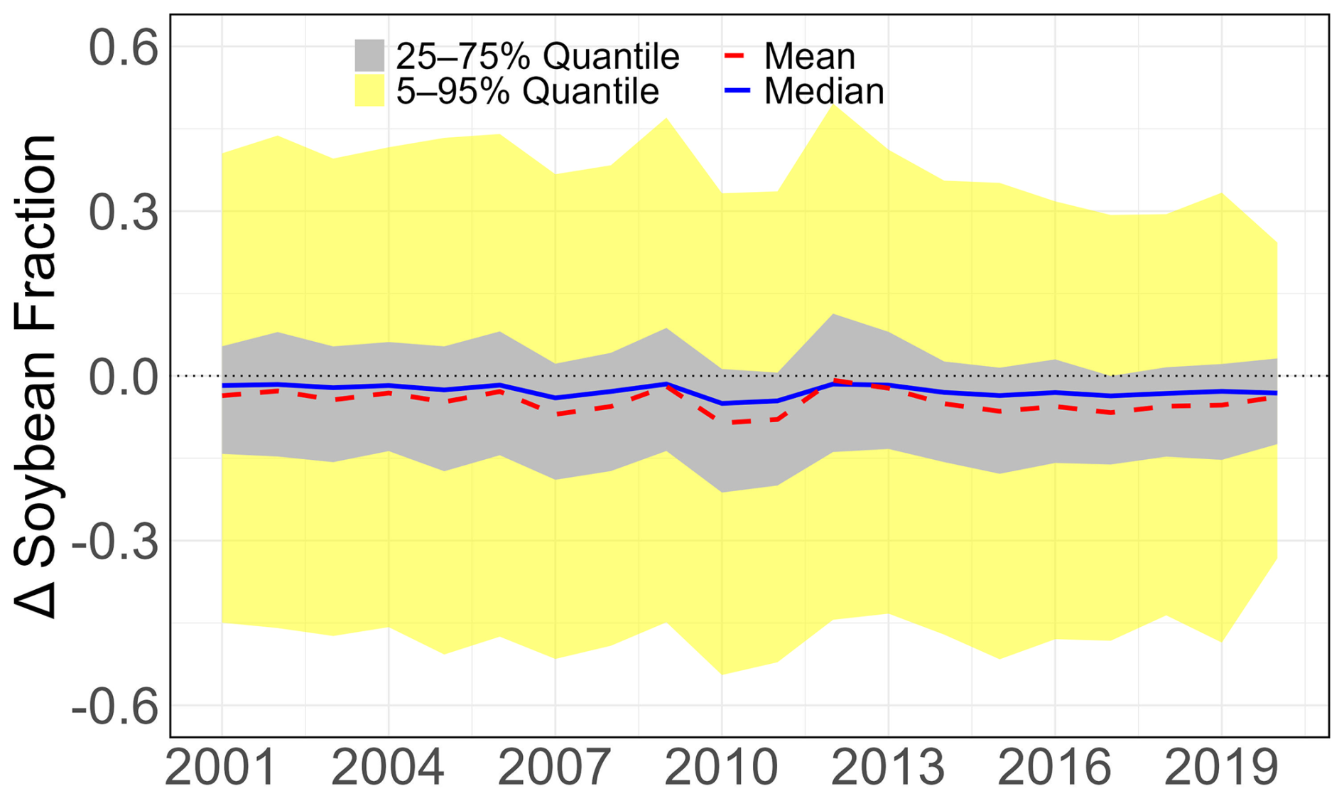
Figure 13 Temporal variation in soybean density difference between GLAD and this study (2001–2020).

4.4 Limitations

This study provides a set of crop type data with 1 km × 1 km resolution and annual steps from 1950 to 2020 in South America. The evaluation at different scales (i.e., provincial, municipal, and grid levels) showed that our reconstructed data are comparable to other datasets. However, some limitations and uncertainties remain in this study. (1) The base maps of cropland density and crop types are crucial for constraining the spatial patterns of crops. In general, reconstructing historical crop type distributions requires using the present crop type distribution as a benchmark to project back into the past. In this study, we used several high-resolution remote sensing products (i.e., Argentina MNC, MapBiomas, and Uruguay LC) to construct a base map. However, these datasets do not provide full spatial coverage of South America and are limited to specific years, which introduces spatial gaps and temporal inconsistencies across the region. As a result, we selectively supplemented the base map with SPAM 2010 in areas where high-resolution products were unavailable, despite its coarser resolution. This highlights the pressing need to develop long-term and high-resolution crop type datasets with consistent spatial and temporal coverage at the regional or global scales. Such datasets would greatly enhance the accuracy and reliability of historical crop-specific reconstructions. (2) In some countries, historical agricultural census data are limited. Adequate historical agricultural census data are the basis for the reconstruction of historical spatial data. Although provincial-level data are available in every country, only a few years of data are accessible in some countries due to inconsistencies in national policies and agricultural census years. Even though these data can be reconstructed in various ways (i.e., interpolation) (Li et al., 2023; Mao et al., 2023), some uncertainties remain. Additionally, national-level trends and interpolation methods were used to reconstruct provincial-level data, which to some extent may miss internal trends of some provinces. Interannual variability at the provincial level is generally not fully consistent with that at the national level, and such reconstruction methods may introduce some overestimation or underestimation of the results. (3) Cropping practice complexity (e.g., crop rotation and multiple cropping) poses a significant challenge for accurate crop distribution mapping. These practices can substantially influence both the spatial patterns and intensity of agriculture land use. Crop rotation, the practice of growing different crops in the same field across multiple years, contributes to soil health, pest control, and long-term cropland management. Ye et al. (2024) considered crop rotation to reconstruct the historical crop distribution maps for the United States, relying on Cropland Data Layer (CDL) data for crop rotation information; however, similar high-resolution products are lacking for South America. In addition, Pott et al. (2023) visualized crop rotation information for soybean, maize, and rice in Rio Grande do Sul, southern Brazil, but it did not sufficiently represent the overall rotation patterns across South America. In contrast, multiple cropping involves the cultivation of more than one crop within the same year in the same field. This practice is common in regions with favorable climate conditions and contributes significantly to agricultural intensity. However, our current method does not differentiate between single-season and multi-season cropping systems, which limits its ability to reflect cropping intensity in areas with prevalent double and triple cropping. Therefore, future research should focus on crop type mapping in South America to obtain crop rotation and multiple cropping patterns, enabling the generation of more accurate historical crop-specific maps in subsequent versions. (4) Crop yield was not considered in this version of dataset. While harvested area provides valuable insights into land use patterns, crop yield remains a critical variable for assessing agricultural production and food security. Accurately reconstructing historical crop yields would require multiple additional factors, including cropping systems (e.g., rainfed or irrigated), input use, farm scale, climate, and weather data. However, such data are generally unavailable or lack consistency across long-term and sub-national scales in South America, particularly before the 2000s. As a result, this version of the dataset focuses exclusively on harvested areas. Future developments could explore the integration of satellite-derived biophysical indicators (e.g., NDVI, LAI), historical production statistics, and climatic data to support the reconstruction of spatial–temporal yield dynamics. (5) There are limitations in representing socioeconomic and environmental drivers. While our data provide long-term, annually resolved reconstructions of crop-specific harvested areas, we did not consider the explicit socioeconomic and environmental drivers such as soil conditions, management practices, or market access. However, incorporating such factors into a harmonized reconstruction presents considerable challenges. First, long-term, high-resolution data on these drivers are unavailable or inconsistently reported across countries. Second, the effects of these drivers are typically region-specific, non-linear, and time-lagged, which poses challenges for systematic modeling. Third, integrating them would require strong assumptions, potentially introducing additional uncertainties into the reconstruction. As a result, our current framework relies on observed statistical records to ensure internal consistency over time but may be less responsive to abrupt cropland shifts induced by major policy or market events. Future improvements could explore the integration of these factors into a hybrid modeling framework (e.g., machine learning or statistical downscaling models such as the GAEZ crop suitability layers) to improve the spatial and temporal realism of crop allocation patterns. Despite these limitations and uncertainties, this study is still the first attempt at crop type reconstruction in South America and has significant implications for analyzing the impacts of agricultural expansion on local livelihoods and food security, trade, and agricultural support policies.

5 Code and data availability

The developed dataset and codes are available at https://doi.org/10.5281/zenodo.14002960 (Xu et al., 2024). The annual and 1 km crop-specific gridded data are in GeoTiff format. The state mask with shapefile and GeoTiff formats is also provided.

6 Conclusions

In this study, we developed spatially explicit crop-specific maps (i.e., soybean, maize, wheat, and rice) at a 1 km × 1 km resolution and annual step in South America from 1950 to 2020 by integrating historical agricultural census data, model-based crop type data, and high-resolution remote-sensing-based crop type data. The results showed that agricultural expansion has severely encroached on the other vegetation of South America over the past 70 years. Specifically, soybean is one of the most dramatically expanded crops, increasing from essentially zero in 1950 to 48.8 Mha in 2020, resulting in a total loss of 23.92 Mha of other vegetation. Additionally, the maize area in South America had increased from 12.7 Mha in 1950 to 26.9 Mha in 2020, encroaching on a total of 18.35 Mha of other vegetation. In contrast, the area of wheat and rice kept relatively stable. Compared with existing data, our reconstructed data have higher spatial and temporal resolution which can better capture the dynamics of crop type changes during the historical period. Overall, this newly developed data can be used to assess the impacts of agricultural expansion on greenhouse gas emissions, ecosystem services, and biodiversity loss and to guide the formulation of land management and conservation policies for sustainable agricultural development and ecological conservation.